On a modified Hilbert transformation,
the discrete inf-sup condition, and error estimates

Abstract

In this paper, we analyze the discrete inf-sup condition and related error estimates for a modified Hilbert transformation as used in the space-time discretization of time-dependent partial differential equations. It turns out that the stability constant depends linearly on the finite element mesh parameter, but in most cases, we can show optimal convergence. We present a series of numerical experiments which illustrate the theoretical findings.

1 Introduction

The Hilbert transformation ${\mathcal{H}}$, e.g., [4, 11], is a useful tool in the mathematical analysis of parabolic evolution equations, e.g., [1, 7]. The particular feature is that the space-time bilinear form $\langle\partial_{t}u,{\mathcal{H}}v\rangle$ is symmetric and elliptic, and therefore allows for the use of standard arguments in the numerical analysis of related space-time finite element methods [5, 13] on the unbounded time interval $(0,\infty)$. While the Hilbert transformation ${\mathcal{H}}$ is defined as Cauchy principal value over ${\mathbb{R}}$, we have recently introduced a modified Hilbert transformation ${\mathcal{H}}_{T}$ acting on a finite time interval $(0,T)$ in [20, 25]. The relation between the modified transformation ${\mathcal{H}}_{T}$ and the classical one was recently given in [6, 18]. In [20, 25], we have analyzed a related space-time finite element method for the numerical solution of a heat equation with zero initial and Dirichlet boundary conditions as a model problem. Extensions include temporal $hp$ approaches and graded meshes in space [16], space-time finite element methods for the Maxwell’s equations [10], and the design of efficient direct solution methods [12]. While in the continuous case we were able to establish an inf-sup stability condition as an ingredient to ensure unique solvability of the space-time variational formulation, the derivation of error estimates for the space-time finite element approximation on tensor-product meshes used the ellipticity estimate for the temporal part only. Indeed, numerical results in [25, Remark 3.4.29] indicate that there does not hold a discrete inf-sup stability condition which is uniform in the space-time finite element mesh size $h$, although we have observed optimal orders of convergence.

When considering the formulation of boundary integral equations for the wave equation in one space dimension, the composition of the modified Hilbert transformation ${\mathcal{H}}_{T}$ with the acoustic single layer boundary integral operator $V$ becomes self-adjoint and elliptic, see [19]. This was the motivation to consider a space-time finite element method for the wave equation using the modified Hilbert transformation ${\mathcal{H}}_{T}$ applied to the test function. While we could ensure unique solvability for any choice of conforming space-time finite element spaces, at that time we were not able to prove convergence, although we have observed optimal rates of convergence in our numerical examples [14]. Again, and as in the parabolic case, numerical results indicate, that the related discrete inf-sup stability condition does not hold uniformly in the space-time finite element mesh size.

The question of analyzing the finite element error in the case when the discrete inf-sup stability condition does not hold uniformly in the finite element mesh size is well studied in the literature, see, e.g., the recent work [3], and the references given therein. In engineering, this is known as patch test, e.g., [2, 28], but also some limitations are well documented, e.g., [22, 23].

In this paper, we consider a modified Hilbert transformation based projection, i.e., a Galerkin projection on piecewise polynomials where the test functions involve the modified Hilbert transformation $\mathcal{H}_{T}$. This requires the analysis of the temporal bilinear form $\langle u,{\mathcal{H}}_{T}v\rangle_{L^{2}(0,T)}$ which is non-negative for $u=v$, and which is a necessary ingredient in the numerical analysis of space-time variational formulations for parabolic and hyperbolic evolution equations. Numerical results indicate that the constant of the related inf-sup condition is proportional to the finite element mesh size $h$, independent of the polynomial degree of the finite element space. On the other hand, in almost all numerical examples, we observe convergence rates as expected from the approximation properties of the finite element spaces. But in the case of a function with a singularity at the origin $t=0$, we observe a convergence rate that is much less than expected. For ease of presentation, in this paper, we provide a detailed analysis in the case of piecewise constant basis functions only. But this approach can be extended to higher-order polynomial basis functions. In fact, we prove that the discrete inf-sup constant is proportional to the finite element mesh size, as already observed in the numerical examples. Moreover, we are able to characterize the discrete inf-sup constant in terms of the Fourier coefficients of finite element functions with respect to the generating functions of the modified Hilbert transformation ${\mathcal{H}}_{T}$. In a second step, we analyze the projection error $u-u_{h}$ with respect to the error $u-Q_{h}u$ of the standard $L^{2}$ projection $Q_{h}u$. When assuming some regularity on $u$, we prove some super-convergence for $u_{h}-Q_{h}u$. This is due to an appropriate splitting of $u_{h}-Q_{h}u$, and mapping properties of $Q_{h}{\mathcal{H}}_{T}^{-1}$. In particular for $u\in H^{2}(0,T)$ satisfying $\partial_{t}u(0)=0$, we prove optimal convergence although the discrete inf-sup condition is mesh dependent. In all other cases, we provide a detailed analysis to theoretically explain all convergence results as observed in the numerical examples.

The rest of this paper is organized as follows: In Section 2, we recall the definition of the modified Hilbert transformation ${\mathcal{H}}_{T}$ and its properties. In particular, in Lemma 2.2 we prove that $\langle v,{\mathcal{H}}_{T}v\rangle_{L^{2}(0,T)}>0$ whenever $0\neq v\in H^{s}_{0,}(0,T)$ for some $s\in(0,1]$, i.e., $v$ is more regular than just in $L^{2}(0,T)$. In addition, we also provide an alternative proof for the relation between the modified Hilbert transformation ${\mathcal{H}}_{T}$ and the Hilbert transformation ${\mathcal{H}}$ which is different from what was presented in [6]. The modified Hilbert transformation based projection is introduced in Section 3, see (3.2), and we discuss the application of more standard stability and error estimates. Numerical examples indicate that the discrete inf-sup condition depends linearly on the finite element mesh size $h$, but the error behaves with optimal order in most cases. While these numerical experiments are done for basis functions up to second order, all further considerations are done for piecewise constant basis functions only. In Section 4, we provide a proof for the discrete inf-sup condition with a mesh dependent stability constant, see Theorem 4.6. The stability constant as given in (4.10) includes a dependency on the Fourier coefficients of the finite element function $u_{h}$ which explains the different behavior as observed in the numerical experiments. Related error estimates are then derived in Section 5. With these results, we are able to explain all the convergence results as observed in the numerical experiments. In Section 6, we finish with some conclusions and comments on ongoing work. For completeness, we provide all the details of the more technical computations in the appendix.

2 A modified Hilbert transformation

Let $T>0$ be a given time horizon. For a function $v\in L^{2}(0,T)$, we consider the Fourier series

$$v(t)=\sum\limits_{k=0}^{\infty}v_{k}\sin\left(\left(\frac{\pi}{2}+k\pi\right)\frac{t}{T}\right),\quad t\in(0,T),$$

where the Fourier coefficients are given by

$$v_{k}=\frac{2}{T}\int_{0}^{T}v(t)\sin\left(\left(\frac{\pi}{2}+k\pi\right)\frac{t}{T}\right)dt.$$ (2.1)

With this, we introduce the modified Hilbert transformation ${\mathcal{H}}_{T}\colon\,L^{2}(0,T)\to L^{2}(0,T)$ as, see [20],

$$({\mathcal{H}}_{T}v)(t):=\sum\limits_{k=0}^{\infty}v_{k}\cos\left(\left(\frac{\pi}{2}+k\pi\right)\frac{t}{T}\right),\quad t\in(0,T).$$

Note that by Parseval’s theorem, we have

$$\|{\mathcal{H}}_{T}v\|_{L^{2}(0,T)}^{2}=\|v\|_{L^{2}(0,T)}^{2}=\frac{T}{2}\,\sum\limits_{k=0}^{\infty}v_{k}^{2}\,.$$ (2.2)

The inverse of the modified Hilbert transformation ${\mathcal{H}}_{T}^{-1}\colon\,L^{2}(0,T)\to L^{2}(0,T)$ is given by

$$({\mathcal{H}}_{T}^{-1}w)(t)=\sum\limits_{k=0}^{\infty}\overline{w}_{k}\sin\left(\left(\frac{\pi}{2}+k\pi\right)\frac{t}{T}\right),\quad t\in(0,T),$$

where

$$\overline{w}_{k}=\frac{2}{T}\int_{0}^{T}w(t)\cos\left(\left(\frac{\pi}{2}+k\pi\right)\frac{t}{T}\right)dt$$ (2.3)

are the coefficients of the Fourier series

$$w(t)=\sum\limits_{k=0}^{\infty}\overline{w}_{k}\cos\left(\left(\frac{\pi}{2}+k\pi\right)\frac{t}{T}\right),\quad t\in(0,T),$$ (2.4)

of a function $w\in L^{2}(0,T)$. As in [20, Lemma 2.4], we have

$$\langle{\mathcal{H}}_{T}u,w\rangle_{L^{2}(0,T)}=\langle u,{\mathcal{H}}_{T}^{-1}w\rangle_{L^{2}(0,T)}\quad\mbox{for all}\;u,w\in L^{2}(0,T).$$ (2.5)

In fact, ${\mathcal{H}}_{T}\colon\,L^{2}(0,T)\to L^{2}(0,T)$ is an isometry, which implies the inf-sup stability condition

$$\|u\|_{L^{2}(0,T)}=\sup\limits_{0\neq v\in L^{2}(0,T)}\frac{\langle u,{\mathcal{H}}_{T}v\rangle_{L^{2}(0,T)}}{\|v\|_{L^{2}(0,T)}}\quad\mbox{for all}\;u\in L^{2}(0,T).$$

We denote by $H^{s}(0,T)$ for $s>0$ the usual Sobolev spaces with norm $\|\cdot\|_{H^{s}(0,T)}$. Further, we define the closed subspaces

$$H^{1}_{0,}(0,T):=\{v\in H^{1}(0,T):v(0)=0\},\quad H^{1}_{,0}(0,T):=\{v\in H^{1}(0,T):v(T)=0\}$$

of $H^{1}(0,T)$ endowed with the Hilbertian norms $\|\cdot\|_{H^{1}_{0,}(0,T)}:=\|\cdot\|_{H^{1}_{,0}(0,T)}:=\|\partial_{t}(\cdot)\|_{L^{2}(0,T)}$ and, we introduce the interpolation spaces

$$H^{s}_{0,}(0,T):=[H^{1}_{0,}(0,T),L^{2}(0,T)]_{s},\quad H^{s}_{,0}(0,T):=[H^{1}_{,0}(0,T),L^{2}(0,T)]_{s}$$

for $s\in(0,1)$, see [25, Section 2.2] for further references. We equip these interpolation spaces with the norms in Fourier representation, i.e.,

$$\|v\|_{H^{s}_{0,}(0,T)}:= \left(\frac{T}{2}\sum\limits_{k=0}^{\infty}\left[\frac{1}{T}\left(\frac{\pi}{2}+k\pi\right)\right]^{2s}v_{k}^{2}\right)^{1/2},$$

$$\|w\|_{H^{s}_{,0}(0,T)}:= \left(\frac{T}{2}\sum\limits_{k=0}^{\infty}\left[\frac{1}{T}\left(\frac{\pi}{2}+k\pi\right)\right]^{2s}\overline{w}_{k}^{2}\right)^{1/2}$$

for $v\in H^{s}_{0,}(0,T)$ with Fourier coefficients $v_{k}$ given in (2.1), and $w\in H^{s}_{,0}(0,T)$ with Fourier coefficients $\overline{w}_{k}$ given in (2.3). Further, for $s\in(0,1)$, $\langle\cdot,\cdot\rangle_{(0,T)}$ denotes the duality pairing in $H^{s}_{,0}(0,T)$ and $[H^{s}_{,0}(0,T)]^{\prime}$ as continuous extension of the $L^{2}(0,T)$ inner product $\langle\cdot,\cdot\rangle_{L^{2}(0,T)}$. Here, for $s\in(0,1)$, the dual space $[H^{s}_{,0}(0,T)]^{\prime}$ is endowed with the norm

$$\|z\|_{[H^{s}_{,0}(0,T)]^{\prime}}=\sup_{0\neq w\in H^{s}_{,0}(0,T)}\frac{\langle z,w\rangle_{(0,T)}}{\|w\|_{H^{s}_{,0}(0,T)}},\quad z\in[H^{s}_{,0}(0,T)]^{\prime}.$$

With this notation, we have the ellipticity

$$\langle\partial_{t}v,{\mathcal{H}}_{T}v\rangle_{(0,T)}\,=\,\|v\|^{2}_{H^{1/2}_{0,}(0,T)}\quad\mbox{for all}\;v\in H^{1/2}_{0,}(0,T),$$

see [20, Equation (2.9)]. Further, for $s\in[0,1]$, the modified Hilbert transformation is an isometry as mapping $\mathcal{H}_{T}\colon\,H^{s}_{0,}(0,T)\to H^{s}_{,0}(0,T)$, satisfying

$$\|\mathcal{H}_{T}v\|_{H^{s}_{,0}(0,T)}=\|v\|_{H^{s}_{0,}(0,T)}\quad\text{for all }v\in H^{s}_{0,}(0,T),$$

which implies a second inf-sup stability condition,

$$\|u\|_{[H^{1/2}_{,0}(0,T)]^{\prime}}=\sup\limits_{0\neq v\in H^{1/2}_{0,}(0,T)}\frac{\langle u,{\mathcal{H}}_{T}v\rangle_{(0,T)}}{\|v\|_{H^{1/2}_{0,}(0,T)}}\quad\mbox{for all}\;u\in[H^{1/2}_{,0}(0,T)]^{\prime}.$$

Remark 2.1

Note that for $0\neq u\in L^{2}(0,T)$, the function $\overline{v}(t):=\int_{0}^{t}u(s)\,ds$, $t\in(0,T)$, yields

$$\langle u,{\mathcal{H}}_{T}\overline{v}\rangle_{(0,T)}=\langle\partial_{t}\overline{v},{\mathcal{H}}_{T}\overline{v}\rangle_{(0,T)}=\|\overline{v}\|^{2}_{H^{1/2}_{0,}(0,T)} =\|\overline{v}\|_{H^{1/2}_{0,}(0,T)}\|\partial_{t}\overline{v}\|_{[H^{1/2}_{,0}(0,T)]^{\prime}}$$

$$=\|\overline{v}\|_{H^{1/2}_{0,}(0,T)}\|u\|_{[H^{1/2}_{,0}(0,T)]^{\prime}}$$

and thus,

$$\|u\|_{[H^{1/2}_{,0}(0,T)]^{\prime}}=\frac{\langle u,{\mathcal{H}}_{T}\overline{v}\rangle_{(0,T)}}{\|\overline{v}\|_{H^{1/2}_{0,}(0,T)}}=\sup\limits_{0\neq v\in H^{1/2}_{0,}(0,T)}\frac{\langle u,{\mathcal{H}}_{T}v\rangle_{(0,T)}}{\|v\|_{H^{1/2}_{0,}(0,T)}}.$$

In [20, Lemma 2.6], it was shown that

$$\langle v,{\mathcal{H}}_{T}v\rangle_{L^{2}(0,T)}\geq 0\quad\mbox{for all}\;v\in L^{2}(0,T).$$

In fact, for a bit more regular functions, we have the following result:

Lemma 2.2

For $0\neq v\in H^{s}_{0,}(0,T)=[H^{1}_{0,}(0,T),L^{2}(0,T)]_{s}$ with $s\in(0,1]$, the inequality

$$\langle v,{\mathcal{H}}_{T}v\rangle_{L^{2}(0,T)}>0$$

holds true.

Proof. By using the representations

$$v(t)=\sum\limits_{k=0}^{\infty}v_{k}\sin\left(\Big{(}\frac{\pi}{2}+k\pi\Big{)}\frac{t}{T}\right),\quad({\mathcal{H}}_{T}v)(t)=\sum\limits_{\ell=0}^{\infty}v_{\ell}\cos\left(\Big{(}\frac{\pi}{2}+\ell\pi\Big{)}\frac{t}{T}\right),$$

it follows from the proof of [20, Lemma 2.6] that

$$\langle v,{\mathcal{H}}_{T}v\rangle_{L^{2}(0,T)}=\frac{T}{\pi}\lim_{N\to\infty}\left[\int_{0}^{1}\left(\sum\limits_{i=0}^{N}v_{2i}x^{2i}\right)^{2}dx+\int_{0}^{1}\left(\sum\limits_{i=0}^{N}v_{2i+1}x^{2i+1}\right)^{2}dx\right].$$ (2.6)

To interchange the limit processes and integral signs in (2.6), the Theorem of Lebesgue is applied. For the first part in (2.6), define the functions

$$f_{1,N}\colon\,(0,1)\to[0,\infty],\quad f_{1,N}(x):=\left(\sum\limits_{i=0}^{N}v_{2i}x^{2i}\right)^{2}\quad\text{for }N\in\mathbb{N}_{0},$$

and

$$f_{1}\colon\,(0,1)\to[0,\infty],\quad f_{1}(x):=\left(\sum\limits_{i=0}^{\infty}v_{2i}x^{2i}\right)^{2}.$$

The Cauchy–Schwarz inequality yields

$$f_{1,N}(x)=|f_{1,N}(x)|\leq\frac{T^{1-2s}}{2}\sum\limits_{i=0}^{\infty}v_{2i}^{2}\left(\frac{\pi}{2}+2i\pi\right)^{2s}\frac{2}{T^{1-2s}}\sum\limits_{i=0}^{\infty}\frac{x^{4i}}{\left(\frac{\pi}{2}+2i\pi\right)^{2s}}\leq\|v\|_{H^{s}_{0,}(0,T)}^{2}\cdot g_{1}(x)$$

for all $x\in(0,1)$ and for all $N\in\mathbb{N}_{0}$, where

$$g_{1}\colon\,[-1,1]\to[0,\infty],\quad g_{1}(x):=\frac{2}{T^{1-2s}}\sum\limits_{i=0}^{\infty}\frac{x^{4i}}{\left(\frac{\pi}{2}+2i\pi\right)^{2s}}=\frac{2^{2s+1}}{T^{1-2s}\pi^{2s}}\sum\limits_{i=0}^{\infty}\frac{x^{4i}}{\left(1+4i\right)^{2s}}.$$

For $x\in(-1,1)$, the estimates

$$0\leq\sum\limits_{i=0}^{\infty}\frac{x^{4i}}{\left(1+4i\right)^{2s}}\leq\sum\limits_{i=0}^{\infty}(x^{4})^{i}=\frac{1}{1-x^{4}}$$

hold true, i.e., the power series $\sum\limits_{i=0}^{\infty}\frac{x^{4i}}{\left(1+4i\right)^{2s}}$ converges absolutely for $x\in(-1,1)$. Hence, for any $y\in(0,1)$, termwise integration is applicable and gives

$$\int_{0}^{y}|g_{1}(x)|dx=\frac{2^{2s+1}}{T^{1-2s}\pi^{2s}}\sum\limits_{i=0}^{\infty}\int_{0}^{y}\frac{x^{4i}}{\left(1+4i\right)^{2s}}dx=\frac{2^{2s+1}}{T^{1-2s}\pi^{2s}}\sum\limits_{i=0}^{\infty}\frac{y^{4i+1}}{\left(1+4i\right)^{2s+1}},$$

where all occurring series converge absolutely. For the endpoint $y=1$, we have that the series $\sum\limits_{i=0}^{\infty}\frac{1}{\left(1+4i\right)^{2s+1}}$ converges if and only if $s>0$, since it can be estimated by general harmonic series. Hence, Abel’s Theorem is applicable, which states

$$\int_{0}^{1}|g_{1}(x)|dx=\lim_{y\to 1^{-}}\int_{0}^{y}|g_{1}(x)|dx=\frac{2^{2s+1}}{T^{1-2s}\pi^{2s}}\sum\limits_{i=0}^{\infty}\frac{1}{\left(1+4i\right)^{2s+1}}.$$

In other words, the function $g_{1}$ is integrable on the interval $(0,1)$ if and only if $s>0.$ Analogous results hold true for the second part in (2.6) with the involved functions

$$f_{2,N}\colon\,(0,1)\to[0,\infty],\quad f_{2,N}(x):=\left(\sum\limits_{i=0}^{N}v_{2i+1}x^{2i+1}\right)^{2}\quad\text{for }N\in\mathbb{N}_{0},$$

$$f_{2}\colon\,(0,1)\to[0,\infty],\quad f_{2}(x):=\left(\sum\limits_{i=0}^{\infty}v_{2i+1}x^{2i+1}\right)^{2}$$

and the function $g_{2}\colon\,[-1,1]\to[0,\infty],$

$$g_{2}(x):=\frac{2}{T^{1-2s}}\sum\limits_{i=0}^{\infty}\frac{x^{4i+2}}{\left(\frac{\pi}{2}+(2i+1)\pi\right)^{2s}}=\frac{2^{2s+1}}{T^{1-2s}\pi^{2s}}\sum\limits_{i=0}^{\infty}\frac{x^{4i+2}}{\left(1+(4i+2)\right)^{2s}},$$

which is integrable on $(0,1)$ if and only if $s>0.$ Summarizing, all assumptions of the Theorem of Lebesgue are satisfied for (2.6). Thus, interchanging the limit processes and integral signs in (2.6) gives

$$\langle v,{\mathcal{H}}_{T}v\rangle_{L^{2}(0,T)}=\frac{T}{\pi}\left[\int_{0}^{1}\left(\sum\limits_{i=0}^{\infty}v_{2i}x^{2i}\right)^{2}dx+\int_{0}^{1}\left(\sum\limits_{i=0}^{\infty}v_{2i+1}x^{2i+1}\right)^{2}dx\right].$$

The last line is strictly positive, since otherwise, the relation

$$\forall x\in(0,1)\colon\quad\sum\limits_{i=0}^{\infty}v_{2i}x^{2i}=\sum\limits_{i=0}^{\infty}v_{2i+1}x^{2i+1}=0$$

would lead, by the Identity Theorem of Power Series, to $v_{k}=0$ for all $k\in\mathbb{N}_{0}$, i.e., a contradiction to $v\neq 0$.  

For $v\in L^{2}(0,T)$, the closed representation [21, Lemma 2.1]

$$({\mathcal{H}}_{T}v)(t)=\frac{1}{2T}\,\mathrm{v.p.}\int_{0}^{T}\left[\frac{1}{\sin\left(\frac{\pi}{2}\frac{s-t}{T}\right)}+\frac{1}{\sin\left(\frac{\pi}{2}\frac{s-t}{T}\right)}\right]\,v(s)\,ds\quad\mbox{for}\;t\in(0,T)$$

as Cauchy principal value holds true, where additional integral representations are contained in [27]. Recall that the classical Hilbert transformation [4] is given as

$$({\mathcal{H}}\varphi)(t)=\frac{1}{\pi}\,\mathrm{v.p.}\int_{\mathbb{R}}\frac{\varphi(s)}{t-s}\,ds\quad\mbox{for}\;t\in\mathbb{R}.$$

In [18, Lemma 4.1], it was shown that the modified Hilbert transformation ${\mathcal{H}}_{T}$ differs from the classical Hilbert transformation ${\mathcal{H}}$ by a compact perturbation $B\colon\,L^{2}(0,T)\to H^{1}(0,T)$, i.e.,

$$({\mathcal{H}}_{T}\varphi)(t)=-({\mathcal{H}}\overline{\varphi})(t)+(B\varphi)(t),\quad t\in(0,T),$$

where

$$\overline{\varphi}(s):=\left\{\begin{array}[]{lcl}\varphi(s)&&\mbox{for}\;s\in(0,T),\\[2.84526pt] \varphi(2T-s)&&\mbox{for}\;s\in(T,2T),\\[2.84526pt] -\varphi(-s)&&\mbox{for}\;s\in(-T,0),\\[2.84526pt] -\varphi(2T+s)&&\mbox{for}\;s\in(-2T,-T),\\[2.84526pt] 0&&\mbox{otherwise}\end{array}\right.$$

is a double reflection of the given function $\varphi\in L^{2}(0,T)$. As it was recently shown in [6], the modified Hilbert transformation ${\mathcal{H}}_{T}$ coincides with the classical Hilbert transformation ${\mathcal{H}}$, when the extension of $\varphi\in L^{2}(0,T)$ is defined accordingly. While there are already three different proofs of this property in [6], here, we present a different way of proof. To this end, we introduce some useful notation. Namely, we denote for $k\in{\mathbb{Z}}$ by

$$\mathcal{E}_{o}\varphi(t):=\left\{\begin{array}[]{lcl}\varphi(s-4kT)&&\mbox{for}\;s\in[4kT,(4k+1)T),\\[2.84526pt] \varphi((4k+2)T-s)&&\mbox{for}\;s\in[(4k+1)T,(4k+2)T),\\[2.84526pt] -\varphi(4kT-s)&&\mbox{for}\;s\in[(4k-1)T,4kT),\\[2.84526pt] -\varphi(s-(4k-2)T)&&\mbox{for}\;s\in[(4k-2)T,(4k-1)T)\end{array}\right.$$

the odd extension of a given function $\varphi\in L^{2}(0,T)$ to a function on $\mathbb{R}$. In particular, note that

$$\mathcal{E}_{o}\sin\left(\Big{(}\frac{\pi}{2}+k\pi\Big{)}\frac{\cdot}{T}\right)(t)=\sin\left(\Big{(}\frac{\pi}{2}+k\pi\Big{)}\frac{t}{T}\right),\quad t\in\mathbb{R}.$$ (2.7)

Moreover, denote the restriction operator by $\mathcal{R}_{(0,T)}\widetilde{\varphi}(t)=\widetilde{\varphi}_{|(0,T)}(t)$, $t\in(0,T)$, for a function $\widetilde{\varphi}\colon\,\mathbb{R}\to\mathbb{R}$. Then, the modified Hilbert transformation admits the representation

$$\mathcal{H}_{T}\varphi=-\mathcal{R}_{(0,T)}\mathcal{H}\mathcal{E}_{o}\varphi\quad\text{for }\varphi\in L^{2}(0,T).$$

To prove this, recall that each $\varphi\in L^{2}(0,T)$ admits the representation

$$\varphi(t)=\sum_{k=0}^{\infty}\varphi_{k}\sin\left(\Big{(}\frac{\pi}{2}+k\pi\Big{)}\frac{t}{T}\right),\quad\varphi_{k}=\frac{2}{T}\int_{0}^{T}\varphi(t)\sin\left(\Big{(}\frac{\pi}{2}+k\pi\Big{)}\frac{t}{T}\right)\,dt.$$

It is well-known that $(\mathcal{H}\sin(a\cdot))(t)=-\cos(at)$ for $t\in\mathbb{R}$ and $a>0$, see [11, (3.110), p. 103]. Using this, and (2.7), we compute that

$$(\mathcal{H}\mathcal{E}_{o}\varphi)(t) =\Big{(}\mathcal{H}\mathcal{E}_{o}\sum_{k=0}^{\infty}\varphi_{k}\sin\left(\Big{(}\frac{\pi}{2}+k\pi\Big{)}\frac{\cdot}{T}\right)(t)\,=\,\sum_{k=0}^{\infty}\varphi_{k}\Big{(}\mathcal{H}\mathcal{E}_{o}\sin\left(\Big{(}\frac{\pi}{2}+k\pi\Big{)}\frac{\cdot}{T}\right)(t)$$

$$=\sum_{k=0}^{\infty}\varphi_{k}\Big{(}\mathcal{H}\sin\left(\Big{(}\frac{\pi}{2}+k\pi\Big{)}\frac{\cdot}{T}\right)(t)\,=\,-\sum_{k=0}^{\infty}\varphi_{k}\cos\left(\Big{(}\frac{\pi}{2}+k\pi\Big{)}\frac{t}{T}\right)$$

$$=-(\mathcal{H}_{T}\varphi)(t)$$

for $t\in(0,T)$. Analogously, using the even extension, for $k\in{\mathbb{Z}}$,

$$\mathcal{E}_{e}\varphi(t):=\left\{\begin{array}[]{lcl}\varphi(s-4kT)&&\mbox{for}\;s\in[4kT,(4k+1)T),\\[2.84526pt] -\varphi((4k+2)T-s)&&\mbox{for}\;s\in[(4k+1)T,(4k+2)T),\\[2.84526pt] \varphi(4kT-s)&&\mbox{for}\;s\in[(4k-1)T,4kT),\\[2.84526pt] -\varphi(s-(4k-2)T)&&\mbox{for}\;s\in[(4k-2)T,(4k-1)T)\end{array}\right.$$

for which

$$\mathcal{E}_{e}\cos\left(\Big{(}\frac{\pi}{2}+k\pi\Big{)}\frac{\cdot}{T}\right)(t)=\cos\left(\Big{(}\frac{\pi}{2}+k\pi\Big{)}\frac{t}{T}\right),\quad t\in\mathbb{R},$$

together with the cosine expansion

$$\varphi(t)=\sum_{k=0}^{\infty}\overline{\varphi}_{k}\cos\left(\Big{(}\frac{\pi}{2}+k\pi\Big{)}\frac{t}{T}\right),\quad\overline{\varphi}_{k}=\frac{2}{T}\int_{0}^{T}\varphi(t)\cos\left(\Big{(}\frac{\pi}{2}+k\pi\Big{)}\frac{t}{T}\right)\,dt,$$

and the property that $(\mathcal{H}\cos(a\cdot))(t)=\sin(at)$, $t\in\mathbb{R}$, $a>0$, we derive that

$$\mathcal{H}_{T}^{-1}\varphi=\mathcal{R}_{(0,T)}\mathcal{H}\mathcal{E}_{e}\varphi\quad\text{for }\varphi\in L^{2}(0,T).$$

To check the consistency, note that the Hilbert transformation of even, periodic functions is odd with the same period and vice versa, see [11, Section 4.2]. Thus, the equality

$$\mathcal{E}_{e}\mathcal{R}_{(0,T)}\mathcal{H}\mathcal{E}_{o}\varphi=\mathcal{H}\mathcal{E}_{o}\varphi\quad\text{for }\varphi\in L^{2}(0,T)$$

holds true. Using that $\mathcal{H}^{2}=-\mathrm{id}$, it is easy to check that

$$\mathcal{H}_{T}^{-1}\mathcal{H}_{T}\varphi=-\mathcal{R}_{(0,T)}\mathcal{H}\mathcal{E}_{e}\mathcal{R}_{(0,T)}\mathcal{H}\mathcal{E}_{o}\varphi=-\mathcal{R}_{(0,T)}\mathcal{H}\mathcal{H}\mathcal{E}_{o}\varphi=\varphi\quad\text{for }\varphi\in L^{2}(0,T).$$

The relation $\mathcal{H}_{T}\mathcal{H}_{T}^{-1}\varphi=\varphi$ for $\varphi\in L^{2}(0,T)$ follows in the same way.

3 A modified Hilbert transformation based projection

For the finite time interval $(0,T)$ and a given discretization parameter $n\in\mathbb{N}$, we consider a uniform decomposition of $(0,T)$ into $n$ finite elements $(t_{i-1},t_{i})$ of mesh size $h=T/n$ with nodes $t_{i}=ih$, $i=0,1,\ldots,n$. With respect to this mesh, we introduce a conforming finite element space

$$V_{h}:=S_{h}^{\nu}(0,T)=\mbox{span}\;\{\psi^{\nu}_{i}\}_{i=1}^{\mathrm{dof}}\subset L^{2}(0,T)$$ (3.1)

of either piecewise constant functions ($\nu=0$ and $\mathrm{dof}=n$) with basis

$$\psi^{0}_{i}(t)=\left\{\begin{array}[]{ccl}1&&\mbox{for}\;t\in(t_{i-1},t_{i}),\\[2.84526pt] 0&&\mbox{otherwise},\end{array}\right.$$

or piecewise linear continuous functions ($\nu=1$ and $\mathrm{dof}=n$) with basis

$$\psi_{i}^{1}(t)=\left\{\begin{array}[]{ccl}(t-t_{i-1})/h&&\mbox{for}\;t\in(t_{i-1},t_{i}],\\[2.84526pt] (t_{i+1}-t)/h&&\mbox{for}\;t\in(t_{i},t_{i+1}),\\[2.84526pt] 0&&\mbox{otherwise}\end{array}\right.$$

for $i=1,\dots,n-1$ and

$$\psi_{n}^{1}(t)=\left\{\begin{array}[]{ccl}(t-t_{n-1})/h&&\mbox{for}\;t\in(t_{n-1},t_{n}],\\[2.84526pt] 0&&\mbox{otherwise},\end{array}\right.$$

or piecewise quadratic continuous functions ($\nu=2$ and $\mathrm{dof}=2n$) fulfilling homogeneous initial conditions. Thus, $S_{h}^{\nu}(0,T)\subset H^{1}_{0,}(0,T)$ for $\nu=1$ or $\nu=2$.

Next, for given $u\in L^{2}(0,T)$, we consider the modified Hilbert transformation based projection to find $u_{h}\in V_{h}$ such that

$$\langle u_{h},{\mathcal{H}}_{T}v_{h}\rangle_{L^{2}(0,T)}=\langle u,{\mathcal{H}}_{T}v_{h}\rangle_{L^{2}(0,T)}\quad\mbox{for all}\;v_{h}\in V_{h}.$$ (3.2)

The variational formulation (3.2) is equivalent to a linear system of algebraic equations,

$$B_{h}^{\nu}\underline{u}=\underline{f}^{\nu},$$

where the Hilbert mass matrix $B_{h}^{\nu}$ is defined by its matrix entries

$$B^{\nu}_{h}[j,i]=\langle\psi^{\nu}_{i},{\mathcal{H}}_{T}\psi^{\nu}_{j}\rangle_{L^{2}(0,T)}\quad\mbox{for}\;i,j=1,\ldots,\mathrm{dof},$$

and the vector $\underline{f}^{\nu}$ of the right-hand side is given by its entries

$$f^{\nu}_{j}=\langle u,{\mathcal{H}}_{T}\psi^{\nu}_{j}\rangle_{L^{2}(0,T)}\quad\mbox{for}\;j=1,\ldots,\mathrm{dof}.$$

Due to Lemma 2.2, we have

$$\underline{v}^{\top}B_{h}^{\nu}\underline{v}=\langle v_{h},{\mathcal{H}}_{T}v_{h}\rangle_{L^{2}(0,T)}>0\quad\mbox{for all}\;\mathbb{R}^{\mathrm{dof}}\ni\underline{v}\leftrightarrow v_{h}\in V_{h},v_{h}\neq 0,$$

from which unique solvability of (3.2) follows. To prove related error estimates, we need to ensure the discrete inf-sup stability condition

$$c_{S}\,\|u_{h}\|_{L^{2}(0,T)}\leq\sup\limits_{0\neq v_{h}\in V_{h}}\frac{\langle u_{h},{\mathcal{H}}_{T}v_{h}\rangle_{L^{2}(0,T)}}{\|v_{h}\|_{L^{2}(0,T)}}\quad\mbox{for all}\;u_{h}\in V_{h}$$ (3.3)

from which we also derive the a priori error estimate [24, Theorem 2], i.e., Céa’s lemma,

$$\|u-u_{h}\|_{L^{2}(0,T)}\leq\frac{1}{c_{S}}\,\inf\limits_{v_{h}\in V_{h}}\|u-v_{h}\|_{L^{2}(0,T)}\,.$$ (3.4)

To motivate our theoretical considerations, let us first consider some numerical examples, where the calculation of the matrix $B^{\nu}_{h}$ and right-hand side $\underline{f}^{\nu}$ is done as proposed in [26]. In Table 1, we present numerical results for the stability constant $c_{S}$ of the inf-sup stability condition (3.3), where for $T=2$, the function $u_{h,\text{min}}$ realizing (3.3) with the smallest inf-sup constant $c_{S}$ is depicted in Figure 1. We observe that $c_{S}$ is mesh dependent. In particular, we have $c_{S}\approx 0.426\cdot h$ for $\nu=0$.

		$\nu=0$		$\nu=1$		$\nu=2$
$n$	$h$	$c_{S}$	$c_{S}/h$	$c_{S}$	$c_{S}/h$	$c_{S}$	$c_{S}/h$
2	1.0	0.411711	0.412	0.515034	0.515	0.429033	0.429
4	0.5	0.211292	0.423	0.344142	0.688	0.271686	0.543
8	0.25	0.106338	0.425	0.204556	0.818	0.155494	0.622
16	0.125	0.053256	0.426	0.112324	0.899	0.083498	0.668
32	0.0625	0.026639	0.426	0.058935	0.943	0.043295	0.693
64	0.03125	0.013321	0.426	0.030192	0.966	0.022047	0.705
128	0.015625	0.006661	0.426	0.015281	0.978	0.011125	0.712
256	0.007812	0.003330	0.426	0.007687	0.984	0.005588	0.715
512	0.003906	0.001665	0.426	0.003855	0.987	0.002800	0.717
1024	0.001953	0.000833	0.426	0.001931	0.988	0.001402	0.718
2048	0.000977	0.000416	0.426	0.000966	0.989	0.000701	0.718

Table 1: Numerical results for the stability constant $c_{S}$ in (3.3) with $T=2$.

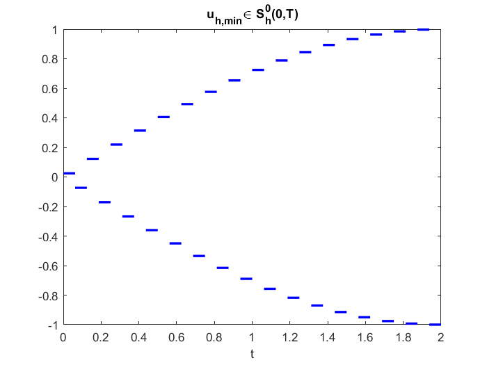
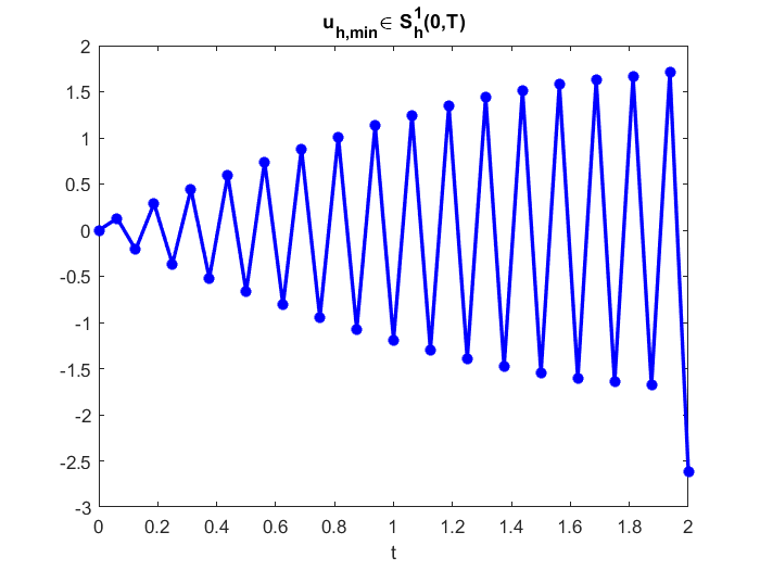
Figure 1: Functions $u_{h,\text{min}}$ realizing (3.3) with the smallest inf-sup constant $c_{S}$ for $N=32$ elements for $T=2$.

From (3.4) and using the approximation properties of $V_{h}$ when assuming $u\in H^{s}(0,T)$ for $s\in[0,\nu+1]$, we then conclude the error estimate

$$\|u-u_{h}\|_{L^{2}(0,T)}\leq c\,h^{s-1}\,\|u\|_{H^{s}(0,T)}\,,$$

in particular, we may lose one order in $h$. However, numerical results indicate a rather different error behavior. As a first example, we consider the regular function $u(t)=\sin\big{(}\frac{\pi}{4}t\big{)}$ for $t\in(0,T)$ with $T=2$, where we observe the optimal order of convergence as expected from the approximation properties of $V_{h}$, see Table 2.

	$\nu=0$		$\nu=1$		$\nu=2$
$n$	$\|u-u_{h}\|_{L^{2}(0,T)}$	eoc	$\|u-u_{h}\|_{L^{2}(0,T)}$	eoc	$\|u-u_{h}\|_{L^{2}(0,T)}$	eoc
2	3.983 –1		2.605 –2		3.893 –3
4	1.825 –1	1.13	5.933 –3	2.13	5.465 –4	2.83
8	8.971 –2	1.02	1.448 –3	2.03	7.051 –5	2.95
16	4.475 –2	1.00	3.599 –4	2.01	8.885 –6	2.99
32	2.238 –2	1.00	8.984 –5	2.00	1.113 –6	3.00
64	1.120 –2	1.00	2.245 –5	2.00	1.392 –7	3.00
128	5.599 –3	1.00	5.613 –6	2.00	1.740 –8	3.00
256	2.800 –3	1.00	1.403 –6	2.00	2.175 –9	3.00
512	1.400 –3	1.00	3.508 –7	2.00	2.719 –10	3.00
1024	7.001 –4	1.00	8.769 –8	2.00	3.398 –11	3.00
2048	3.501 –4	1.00	2.192 –8	2.00	4.236 –12	3.00

Table 2: Error for the regular function $u(t)=\sin\big{(}\frac{\pi}{4}t\big{)}$, $t\in(0,T)$, with $T=2$.

As a second example, we consider $u(t)=t^{2/3}$ for $t\in(0,T)$ and $T=2$ with a singular behavior at $t=0$, i.e., $u\in H^{7/6-\varepsilon}_{0,}(0,T)$ for any $\varepsilon\in(0,1)$. Here, we observe a convergence order of $\frac{2}{3}$ for $\nu\in\{0,1,2\}$, which for $\nu=1$, is between the expected order $\frac{1}{6}$ and the optimal approximation order $\frac{7}{6}$, see Table 3.

	$\nu=0$		$\nu=1$		$\nu=2$
$n$	$\|u-u_{h}\|_{L^{2}(0,T)}$	eoc	$\|u-u_{h}\|_{L^{2}(0,T)}$	eoc	$\|u-u_{h}\|_{L^{2}(0,T)}$	eoc
2	4.796 –1		1.597 –1		6.268 –2
4	2.921 –1	0.72	9.222 –2	0.79	3.693 –2	0.76
8	1.783 –1	0.71	5.506 –2	0.74	2.237 –2	0.72
16	1.093 –1	0.71	3.369 –2	0.71	1.381 –2	0.70
32	6.741 –2	0.70	2.090 –2	0.69	8.604 –3	0.68
64	4.181 –2	0.69	1.306 –2	0.67	5.391 –3	0.67
128	2.605 –2	0.68	8.195 –3	0.67	3.387 –3	0.67
256	1.628 –2	0.68	5.152 –3	0.67	2.131 –3	0.67
512	1.021 –2	0.67	3.243 –3	0.67	1.341 –3	0.67
1024	6.408 –3	0.67	2.042 –3	0.67	8.447 –4	0.67
2048	4.028 –3	0.67	1.286 –3	0.67	5.320 –4	0.67

Table 3: Error for $u(t)=t^{2/3}$, $t\in(0,T)$, with $T=2$.

As a last example, we consider $u(t)=t(T-t)^{2/3}$, $t\in(0,T)$ with a singular behavior at $t=T=2$. Again, we have $u\in H^{7/6-\varepsilon}_{0,}(0,T)$ but we observe the optimal order of convergence as expected from the approximation property, see Table 4.

	$\nu=0$		$\nu=1$		$\nu=2$
$n$	$\|u-u_{h}\|_{L^{2}(0,T)}$	eoc	$\|u-u_{h}\|_{L^{2}(0,T)}$	eoc	$\|u-u_{h}\|_{L^{2}(0,T)}$	eoc
2	8.327 –1		1.506 –1		3.061 –2
4	3.980 –1	1.07	5.054 –2	1.58	1.221 –2	1.33
8	1.968 –1	1.02	1.823 –2	1.47	5.210 –3	1.23
16	9.852 –2	1.00	7.180 –3	1.34	2.271 –3	1.20
32	4.951 –2	0.99	3.000 –3	1.26	1.001 –3	1.18
64	2.490 –2	0.99	1.295 –3	1.21	4.433 –4	1.17
128	1.252 –2	0.99	5.677 –4	1.19	1.969 –4	1.17
256	6.287 –3	0.99	2.510 –4	1.18	8.760 –5	1.17
512	3.156 –3	0.99	1.114 –4	1.17	3.899 –5	1.17
1024	1.583 –3	1.00	4.952 –5	1.17	1.736 –5	1.17
2048	7.936 –4	1.00	2.204 –5	1.17	7.733 –6	1.17

Table 4: Error for $u(t)=t(T-t)^{2/3}$, $t\in(0,T)$, with $T=2$.

Remark 3.1

When introducing the test space $W_{h}=\{\int_{0}^{\cdot}v_{h}(s)ds\in H^{1}_{0,}(0,T):v_{h}\in V_{h}\}$ with $V_{h}=S_{h}^{\nu}(0,T)$ given in (3.1) for $\nu\in\{0,1,2\}$, and when considering the Galerkin–Petrov variational formulation to find $u_{h}\in V_{h}$ such that

$$\langle u_{h},{\mathcal{H}}_{T}w_{h}\rangle_{L^{2}(0,T)}=\langle u,{\mathcal{H}}_{T}w_{h}\rangle_{L^{2}(0,T)}\quad\mbox{for all}\;w_{h}\in W_{h},$$

we prove, as in Remark 2.1, the discrete inf-sup stability condition

$$\|u_{h}\|_{[H^{1/2}_{,0}(0,T)]^{\prime}}\leq\sup\limits_{0\neq w_{h}\in W_{h}}\frac{\langle u_{h},{\mathcal{H}}_{T}w_{h}\rangle_{L^{2}(0,T)}}{\|w_{h}\|_{H^{1/2}_{0,}(0,T)}}\quad\mbox{for all}\;u_{h}\in V_{h},$$

which also ensures optimal error estimates for the approximate solution $u_{h}$. However, and due to the applications in mind, our main interest is in the numerical stability analysis of the Galerkin–Bubnov formulation (3.2).

4 Discrete inf-sup stability condition in $S_{h}^{0}(0,T)$

For $n$ finite elements, we start by considering a given piecewise constant function $u_{h}\in S_{h}^{0}(0,T)$, i.e.,

$$u_{h}(t)=\sum\limits_{i=1}^{n}u_{i}\psi_{i}^{0}(t),\quad t\in[0,T],$$

with the norm

$$\|u_{h}\|^{2}_{L^{2}(0,T)}=\int_{0}^{T}[u_{h}(t)]^{2}\,dt\,=\,h\,\sum\limits_{i=1}^{n}u_{i}^{2}\,.$$

In addition, we consider its Fourier series, see (2.4),

$$u_{h}(t)=\sum\limits_{k=0}^{\infty}\overline{u}_{k}\cos\left(\Big{(}\frac{\pi}{2}+k\pi\Big{)}\frac{t}{T}\right),\quad\overline{u}_{k}\,=\,\frac{2}{T}\int_{0}^{T}u_{h}(t)\,\cos\left(\Big{(}\frac{\pi}{2}+k\pi\Big{)}\frac{t}{T}\right)\,dt,$$

with the norm representation (2.2),

$$\|u_{h}\|^{2}_{L^{2}(0,T)}=\frac{T}{2}\,\sum\limits_{k=0}^{\infty}\overline{u}_{k}^{2}\,.$$

It turns out that for $u_{h}\in S_{h}^{0}(0,T)$, it is sufficient to use a finite sum of the Fourier coefficients $\overline{u}_{k}^{2}$ to define an equivalent norm. Before we state this result, we need an auxiliary lemma, for which we first define

$$x_{k}:=\left(\frac{\pi}{2}+k\pi\right)\frac{1}{2n}\quad\mbox{for}\;k\in{\mathbb{N}}_{0}.$$ (4.1)

Lemma 4.1

For all $n\in\mathbb{N}$, and for all $k\in\mathbb{N}_{0}$, the equality

$$\sum_{i=1}^{n}\cos^{2}((2i-1)x_{k})\,=\,\sum_{i=1}^{n}\cos^{2}\left(\Big{(}\frac{\pi}{2}+k\pi\Big{)}\frac{2i-1}{2n}\right)\,=\,\frac{n}{2}$$ (4.2)

holds true.

Proof. When using $\cos(2x)=2\cos^{2}x-1$, we write

$$\sum_{i=1}^{n}\cos^{2}\left(\Big{(}\frac{\pi}{2}+k\pi\Big{)}\frac{2i-1}{2n}\right)\,=\,\frac{1}{2}\sum_{i=1}^{n}\left[1+\cos\left(\Big{(}\frac{\pi}{2}+k\pi\Big{)}\frac{2i-1}{n}\right)\right],$$

and the assertion follows when using [8, Equation 1.342, 4.].  

Lemma 4.2

Let $M=n^{2}$. Then, the norm equivalence inequalities

$$\frac{T}{2}\,\sum\limits_{k=0}^{M}\overline{u}_{k}^{2}\leq\|u_{h}\|_{L^{2}(0,T)}^{2}\leq 2\,\left(\frac{T}{2}\,\sum\limits_{k=0}^{M}\overline{u}_{k}^{2}\right)$$ (4.3)

hold true.

Proof. While the lower estimate is trivial, to prove the upper estimate, we first compute the Fourier coefficients

$$\overline{u}_{k}\,=\,\frac{2}{T}\int_{0}^{T}u_{h}(t)\,\cos\left(\Big{(}\frac{\pi}{2}+k\pi\Big{)}\frac{t}{T}\right)\,dt\,=\,\frac{2}{n}\,\frac{\sin x_{k}}{x_{k}}\,\sum\limits_{i=1}^{n}u_{i}\cos((2i-1)x_{k}).$$ (4.4)

Using Hölder’s inequality and (4.2), we estimate

$$\overline{u}_{k}^{2} =\frac{4}{n^{2}}\,\frac{\sin^{2}x_{k}}{x_{k}^{2}}\,\left[\sum\limits_{i=1}^{n}u_{i}\cos\left(\Big{(}\frac{\pi}{2}+k\pi\Big{)}\frac{2i-1}{2n}\right)\right]^{2}$$

$$\leq\frac{4}{n^{2}}\,\frac{\sin^{2}x_{k}}{x_{k}^{2}}\sum\limits_{i=1}^{n}u_{i}^{2}\;\sum\limits_{i=1}^{n}\cos^{2}\left(\Big{(}\frac{\pi}{2}+k\pi\Big{)}\frac{2i-1}{2n}\right)$$

$$=\frac{2}{n}\,\frac{\sin^{2}x_{k}}{x_{k}^{2}}\sum\limits_{i=1}^{n}u_{i}^{2}\,=\,\frac{2}{T}\,\frac{\sin^{2}x_{k}}{x_{k}^{2}}\,\|u_{h}\|^{2}_{L^{2}(0,T)}.$$

Hence, we write

$$\|u_{h}\|^{2}_{L^{2}(0,T)}\,=\,\frac{T}{2}\sum\limits_{k=0}^{\infty}\overline{u}_{k}^{2}\,\leq\,\frac{T}{2}\sum\limits_{k=0}^{M}\overline{u}_{k}^{2}+\sum\limits_{k=M+1}^{\infty}\frac{\sin^{2}x_{k}}{x_{k}^{2}}\,\|u_{h}\|^{2}_{L^{2}(0,T)},$$

and we estimate

$$\sum\limits_{k=M+1}^{\infty}\frac{\sin^{2}x_{k}}{x_{k}^{2}}=\sum\limits_{k=M+1}^{\infty}\frac{\sin^{2}\left(\Big{(}\frac{\pi}{2}+k\pi\Big{)}\frac{1}{2n}\right)}{[(\frac{\pi}{2}+k\pi)\frac{1}{2n}]^{2}}\leq\frac{4n^{2}}{\pi^{2}}\sum\limits_{k=M+1}^{\infty}\frac{1}{k^{2}}\,\leq\,\frac{n^{2}}{2}\,\sum\limits_{k=M+1}^{\infty}\frac{1}{k^{2}}\,.$$

With

$$\sum\limits_{k=M+1}^{\infty}\frac{1}{k^{2}}\leq\int_{M}^{\infty}\frac{1}{x^{2}}\,dx=\left[-\frac{1}{x}\right]_{x=M}^{\infty}=\frac{1}{M},$$

we further conclude

$$\|u_{h}\|^{2}_{L^{2}(0,T)}\leq\frac{T}{2}\sum\limits_{k=0}^{M}\overline{u}_{k}^{2}+\frac{n^{2}}{2}\,\frac{1}{M}\,\|u_{h}\|_{L^{2}(0,T)}^{2},$$

and due to $M=n^{2}$ we obtain the assertion.  

From the norm equivalence inequalities (4.3), we observe that $u_{h}\equiv 0$ if $\overline{u}_{k}=0$ for all $k=0,\ldots,n^{2}$. Thus, all coefficients $\overline{u}_{k}$ for $k>n^{2}$ have to be linear dependent on the coefficients $\overline{u}_{k}$ for $k=0,\ldots,n^{2}$. In the following lemma, we state this relation in more detail. In particular, we prove that the Fourier coefficients $\overline{u}_{k}$ for $k=0,\ldots,n-1$ are sufficient to describe $u_{h}$.

Lemma 4.3

The Fourier coefficients as given in (4.4) satisfy the recurrence relations

$$\overline{u}_{k+2\mu n}=\frac{2k+1}{2k+1+4\mu n}\,\overline{u}_{k}\quad\mbox{for }\;k=0,1,2,\ldots,2n-1,\;\mu\in\mathbb{N},$$ (4.5)

and

$$\overline{u}_{2n-1-k}=-\frac{2k+1}{4n-1-2k}\,\overline{u}_{k}\quad\mbox{for }\;k=0,1,2\ldots,n-1.$$ (4.6)

Proof. The assertion follows from direct computations, we skip the details.  

With this, we are in a position to rewrite the upper norm equivalence inequality in (4.3) in a more appropriate way.

Corollary 4.4

For $u_{h}\in V_{h}=S_{h}^{0}(0,T)$, the estimate

$$\|u_{h}\|_{L^{2}(0,T)}^{2}\leq\frac{T}{2}\,\frac{\pi^{2}}{3}\,\sum\limits_{k=0}^{n-1}\overline{u}_{k}^{2}$$

holds true, where the Fourier coefficients $\overline{u}_{k}$ are given as in (4.4).

Proof. We define

$$\gamma(k,n):=\sum\limits_{\mu=0}^{\infty}\frac{(2k+1)^{2}}{(2k+1+4\mu n)^{2}},$$

satisfying, for $k=0,\ldots,2n-1$,

$$1\leq\gamma(k,n)=\sum\limits_{\mu=0}^{\infty}\frac{(2k+1)^{2}}{(2k+1+4\mu n)^{2}}=\sum\limits_{\mu=0}^{\infty}\frac{(\frac{2k+1}{4n})^{2}}{(\frac{2k+1}{4n}+\mu)^{2}}\leq\sum\limits_{\mu=0}^{\infty}\frac{1}{(1+\mu)^{2}}=\frac{\pi^{2}}{6},$$

where we use that the function $(0,1)\ni y\mapsto\frac{y^{2}}{(y+\mu)^{2}}\in\mathbb{R}$ is non-decreasing. Equation (4.5) gives

$$\sum\limits_{k=0}^{\infty}\overline{u}_{k}^{2}=\sum\limits_{k=0}^{2n-1}\sum\limits_{\mu=0}^{\infty}\overline{u}^{2}_{k+2\mu n}=\sum\limits_{k=0}^{2n-1}\overline{u}_{k}^{2}\sum\limits_{\mu=0}^{\infty}\frac{(2k+1)^{2}}{(2k+1+4\mu n)^{2}}=\sum\limits_{k=0}^{2n-1}\gamma(k,n)\,\overline{u}_{k}^{2}.$$

Next, we employ (4.6) and the transformation $k=2n-1-j$ for $j=0,\ldots,n-1$ to conclude that

$$\sum\limits_{k=0}^{2n-1}\gamma(k,n)\,\overline{u}_{k}^{2} =\sum\limits_{k=0}^{n-1}\gamma(k,n)\,\overline{u}_{k}^{2}+\sum\limits_{k=n}^{2n-1}\gamma(k,n)\,\overline{u}_{k}^{2}$$

$$=\sum\limits_{k=0}^{n-1}\gamma(k,n)\,\overline{u}_{k}^{2}+\sum\limits_{j=0}^{n-1}\gamma(2n-1-j,n)\,\overline{u}_{2n-1-j}^{2}$$

$$=\sum\limits_{k=0}^{n-1}\left[\gamma(k,n)+\gamma(2n-1-k,n)\,\frac{(2k+1)^{2}}{(4n-1-2k)^{2}}\right]\,\overline{u}_{k}^{2}$$

$$\leq\sum\limits_{k=0}^{n-1}\Big{[}\gamma(k,n)+\gamma(2n-1-k,n)\,\Big{]}\,\overline{u}_{k}^{2}\leq\frac{\pi^{2}}{3}\sum\limits_{k=0}^{n-1}\overline{u}_{k}^{2}.$$

When using this within the norm representation (2.2), this gives the assertion.  

Lemma 4.5

Let $n\in\mathbb{N}$ be given. For all $k,\ell=0,\ldots,n-1$, the discrete orthogonality

$$\sum\limits_{i=1}^{n}\sin((2i-1)x_{k})\sin((2i-1)x_{\ell})=\frac{n}{2}\,\delta_{k\ell}$$ (4.7)

holds true.

Proof. For $k=\ell$, the assertion is a simple consequence of (4.2), due to $\sin^{2}=1-\cos^{2}x$. For the remaining case $\ell\neq k$, we have, using $\sin x\sin y=\frac{1}{2}[\cos(x-y)-\cos(x+y)]$,

$$\sum\limits_{i=1}^{n}\sin((2i-1)x_{k})\sin((2i-1)x_{\ell})=\sum\limits_{i=1}^{n}\sin\left(\Big{(}\frac{\pi}{2}+k\pi\Big{)}\frac{2i-1}{2n}\right)\sin\left(\Big{(}\frac{\pi}{2}+\ell\pi\Big{)}\frac{2i-1}{2n}\right)\\ =\,\frac{1}{2}\sum\limits_{i=1}^{n}\left[\cos\left((k-\ell)\pi\frac{2i-1}{2n}\right)-\cos\left((k+\ell+1)\pi\frac{2i-1}{2n}\right)\right],$$

and it is sufficient to prove

$$\sum\limits_{i=1}^{n}\cos\left(\nu\pi\frac{2i-1}{2n}\right)=0$$

for all $\nu=1,\ldots,2n-1$. Using [8, Equation 1.341, 3.] yields

$$\sum_{i=1}^{n}\cos\left(\nu\pi\frac{2i-1}{2n}\right)=\sum_{j=0}^{n-1}\cos\left(\nu\pi\frac{2j+1}{2n}\right)\\ =\underbrace{\cos\left(\nu\pi\frac{1}{2n}+\nu\pi\frac{n-1}{2n}\right)}_{=0}\sin\left(\frac{\nu\pi}{2}\right)\frac{1}{\sin\left(\nu\pi\frac{1}{2n}\right)}=0$$

and thus, the assertion.  

With this, we are in the position to state the main result of this section:

Theorem 4.6

For an arbitrary but fixed $u_{h}\in S_{h}^{0}(0,T)$, we define $w_{h}:=Q_{h}{\mathcal{H}}_{T}^{-1}u_{h}$ as the unique solution of the variational formulation

$$\langle w_{h},v_{h}\rangle_{L^{2}(0,T)}=\langle{\mathcal{H}}_{T}^{-1}u_{h},v_{h}\rangle_{L^{2}(0,T)}\quad\mbox{for all}\;v_{h}\in S_{h}^{0}(0,T).$$ (4.8)

Then, the inf-sup condition

$$c_{S}(u_{h})\,\|u_{h}\|_{L^{2}(0,T)}\leq\frac{\langle u_{h},{\mathcal{H}}_{T}w_{h}\rangle_{L^{2}(0,T)}}{\|w_{h}\|_{L^{2}(0,T)}}$$ (4.9)

holds true with

$$c_{S}(u_{h}):=\frac{2\sqrt{3}}{\pi^{2}}\,\frac{16n^{2}-8n(2M+1)}{(4n-(2M+1))^{2}},$$ (4.10)

where

$$M:=\mbox{\rm arg min}\left\{m\in{\mathbb{N}}:\|u_{h}\|^{2}_{L^{2}(0,T)}\leq\frac{T}{2}\,\frac{\pi^{2}}{3}\,\sum\limits_{k=0}^{m}\overline{u}_{k}^{2}\right\}\leq n-1$$ (4.11)

with the Fourier coefficients $\overline{u}_{k}$ as given in (4.4).

Proof. For a given $u_{h}\in S_{h}^{0}(0,T)$, we first define

$$w(t):={\mathcal{H}}_{T}^{-1}u_{h}(t)=\sum\limits_{k=0}^{\infty}\overline{u}_{k}\sin\left(\Big{(}\frac{\pi}{2}+k\pi\Big{)}\frac{t}{T}\right),$$

where the Fourier coefficients $\overline{u}_{k}$ are as in (4.4). For this, we compute the piecewise constant $L^{2}$ projection

$$w_{h}(t)=Q_{h}{\mathcal{H}}_{T}^{-1}u_{h}(t)=\sum\limits_{j=1}^{n}w_{j}\psi_{j}^{0}(t)$$

as the unique solution of (4.8), from which we conclude

$$w_{j}=\sum\limits_{k=0}^{\infty}\overline{u}_{k}\,\frac{\sin x_{k}}{x_{k}}\,\sin((2j-1)x_{k}),$$ (4.12)

and using (4.5), we write

$$w_{j}=\sum\limits_{k=0}^{2n-1}\overline{u}_{k}\,\gamma(k,n)\,\frac{\sin x_{k}}{x_{k}}\,\sin((2j-1)x_{k}).$$ (4.13)

Next, we use (4.6) to conclude

$$w_{j}=\sum\limits_{k=0}^{n-1}\overline{u}_{k}\Big{[}\gamma(k,n)-\gamma(2n-1-k,n)\frac{(2k+1)^{2}}{(4n-1-2k)^{2}}\Big{]}\,\frac{\sin x_{k}}{x_{k}}\,\sin((2j-1)x_{k}).$$ (4.14)

Using the discrete orthogonality (4.7), it remains to compute

$$\|w_{h} \|^{2}_{L^{2}(0,T)}=h\sum\limits_{j=1}^{n}w_{j}^{2}$$

$$= h\sum\limits_{j=1}^{n}\left\{\sum\limits_{k=0}^{n-1}\overline{u}_{k}\Big{[}\gamma(k,n)-\gamma(2n-1-k,n)\frac{(2k+1)^{2}}{(4n-1-2k)^{2}}\Big{]}\frac{\sin x_{k}}{x_{k}}\sin((2j-1)x_{k})\right\}^{2}$$

$$= \frac{T}{2}\,\sum\limits_{k=0}^{n-1}\overline{u}_{k}^{2}\,\Big{[}\gamma(k,n)-\gamma(2n-1-k,n)\frac{(2k+1)^{2}}{(4n-1-2k)^{2}}\Big{]}^{2}\;\frac{\sin^{2}x_{k}}{x_{k}^{2}}.$$

With $2k+1<4n-(2k+1)$ for $k=0,\ldots,n-1$, we calculate that

$$\gamma(k,n)-\gamma(2n-1-k ,n)\frac{(2k+1)^{2}}{(4n-1-2k)^{2}}$$

$$=\sum\limits_{\mu=0}^{\infty}\frac{(2k+1)^{2}}{(2k+1+4\mu n)^{2}}-\frac{(2k+1)^{2}}{(4n-1-2k)^{2}}\sum\limits_{\mu=0}^{\infty}\frac{(4n-1-2k)^{2}}{(4n-1-2k+4\mu n)^{2}}$$

$$=(2k+1)^{2}\sum\limits_{\mu=0}^{\infty}\left[\frac{1}{(2k+1+4\mu n)^{2}}-\frac{1}{(4n-1-2k+4\mu n)^{2}}\right]$$

$$>(2k+1)^{2}\left[\frac{1}{(2k+1)^{2}}-\frac{1}{(4n-1-2k)^{2}}\right]$$

$$=1-\frac{(2k+1)^{2}}{(4n-1-2k)^{2}}.$$

For $k=0,\ldots,n-1$, we have $x_{k}\in(0,\frac{\pi}{2})$, and therefore,

$$\frac{\sin^{2}x_{k}}{x_{k}^{2}}\geq\frac{4}{\pi^{2}}\quad\mbox{for all}\;k=0,\ldots,n-1.$$

Let $M\leq n-1$ such that (4.11) is satisfied. Then, we write

$$\|w_{h}\|^{2}_{L^{2}(0,T)} >\frac{T}{2}\,\frac{4}{\pi^{2}}\,\sum\limits_{k=0}^{n-1}\overline{u}_{k}^{2}\left[1-\frac{(2k+1)^{2}}{(4n-1-2k)^{2}}\right]^{2}$$

$$\geq\frac{T}{2}\,\frac{4}{\pi^{2}}\,\sum\limits_{k=0}^{M}\overline{u}_{k}^{2}\left[1-\frac{(2k+1)^{2}}{(4n-1-2k)^{2}}\right]^{2}$$

$$\geq\frac{T}{2}\,\frac{4}{\pi^{2}}\,\left[1-\frac{(2M+1)^{2}}{(4n-1-2M)^{2}}\right]^{2}\sum\limits_{k=0}^{M}\overline{u}_{k}^{2}$$

$$\geq\frac{4}{\pi^{2}}\,\frac{3}{\pi^{2}}\left[1-\frac{(2M+1)^{2}}{(4n-1-2M)^{2}}\right]^{2}\,\|u_{h}\|^{2}_{L^{2}(0,T)}$$

$$=\frac{12}{\pi^{4}}\,\left[\frac{16n^{2}-8n(2M+1)}{(4n-(2M+1))^{2}}\right]^{2}\,\|u_{h}\|^{2}_{L^{2}(0,T)},$$

i.e., we conclude that

$$\|w_{h}\|_{L^{2}(0,T)}\,\geq\,\frac{2\sqrt{3}}{\pi^{2}}\,\frac{16n^{2}-8n(2M+1)}{(4n-(2M+1))^{2}}\,\|u_{h}\|_{L^{2}(0,T)}.$$

Due to

$$\langle u_{h},{\mathcal{H}}_{T}w_{h}\rangle_{L^{2}(0,T)}\,=\,\langle{\mathcal{H}}_{T}^{-1}u_{h},w_{h}\rangle_{L^{2}(0,T)}\,=\,\langle w_{h},w_{h}\rangle_{L^{2}(0,T)}\,=\,\|w_{h}\|_{L^{2}(0,T)}^{2},$$

this finally implies the desired estimate.  

Corollary 4.7

The estimate (4.9) implies the inf-sup stability condition

$$c_{S}\,\|u_{h}\|_{L^{2}(0,T)}\leq\sup\limits_{0\neq v_{h}\in S_{h}^{0}(0,T)}\frac{\langle u_{h},{\mathcal{H}}_{T}v_{h}\rangle_{L^{2}(0,T)}}{\|v_{h}\|_{L^{2}(0,T)}}$$

for all $u_{h}\in S_{h}^{0}(0,T)$, where we have to consider $M=n-1$, i.e.,

$$c_{S}:=\min\limits_{u_{h}\in S_{h}^{0}(0,T)}c_{S}(u_{h})=\frac{1}{T}\,\frac{2\sqrt{3}}{\pi^{2}}\,\frac{8}{(2+\frac{1}{n})^{2}}\,h\,.$$

In particular for $T=2$, we have

$$\lim\limits_{n\to\infty}\frac{1}{2}\,\frac{2\sqrt{3}}{\pi^{2}}\,\frac{8}{(2+\frac{1}{n})^{2}}\,=\,\frac{2\sqrt{3}}{\pi^{2}}\,\simeq\,0.351.$$

Note that the value obtained from the numerical experiments as given in Table 1 was $0.426$.

Remark 4.8

In the case of a constant $M$ independent of $n$, we obtain

$$c_{S}(u_{h})\simeq\frac{2\sqrt{3}}{\pi^{2}}$$

independent of the mesh size $h$. In the case $M=n-\sqrt{n}$, this would result in

$$c_{S}(u_{h})=\frac{2\sqrt{3}}{\pi^{2}}\,\frac{16n^{2}-8n(2M+1)}{(4n-(2M+1))^{2}}=\frac{2\sqrt{3}}{\pi^{2}}\,\frac{16n\sqrt{n}-1}{(2n+2\sqrt{n}-1)^{2}}\simeq\frac{8\sqrt{3}}{\pi^{2}}\,\frac{1}{\sqrt{n}}=\frac{8\sqrt{3}}{\pi^{2}\sqrt{T}}\,h^{1/2}\,.$$

5 Error estimates for the projection in $S_{h}^{0}(0,T)$

This section aims to present a numerical analysis in order to confirm the numerical results as presented in Section 3. In addition to the solution $u_{h}\in V_{h}=S_{h}^{0}(0,T)$ of the variational formulation (3.2), we introduce the $L^{2}$ projection $Q_{h}u\in S_{h}^{0}(0,T)$ as unique solution of the variational formulation

$$\langle Q_{h}u,v_{h}\rangle_{L^{2}(0,T)}=\langle u,v_{h}\rangle_{L^{2}(0,T)}\quad\mbox{for all}\;v_{h}\in S_{h}^{0}(0,T).$$ (5.1)

When we assume $u\in H^{s}(0,T)$ for some $s\in[0,1]$, the error estimate

$$\|u-Q_{h}u\|_{L^{2}(0,T)}\leq c\,h^{s}\,\|u\|_{H^{s}(0,T)}$$

holds true, see, e.g., [17]. Using the triangle inequality, we therefore have

$$\|u-u_{h}\|_{L^{2}(0,T)}\leq c\,h^{s}\,\|u\|_{H^{s}(0,T)}+\|u_{h}-Q_{h}u\|_{L^{2}(0,T)},$$ (5.2)

and it remains to estimate the second term.

Lemma 5.1

Let $u_{h}\in S_{h}^{0}(0,T)$ be the unique solution of the variational formulation (3.2), and let $Q_{h}u\in S_{h}^{0}(0,T)$ be the $L^{2}$ projection of $u\in L^{2}(0,T)$ as defined in (5.1). Then, the estimate

$$\|u_{h}-Q_{h}u\|_{L^{2}(0,T)}\leq\frac{1}{c_{S}(u_{h}-Q_{h}u)}\,\|Q_{h}{\mathcal{H}}_{T}^{-1}(u-Q_{h}u)\|_{L^{2}(0,T)}$$ (5.3)

holds true, where $c_{S}(u_{h}-Q_{h}u)$ is the stability constant as defined in (4.10).

Proof. As in Theorem 4.6, we define $w={\mathcal{H}}_{T}^{-1}(u_{h}-Q_{h}u)$ as well as $w_{h}=Q_{h}{\mathcal{H}}_{T}^{-1}(u_{h}-Q_{h}u)$. From the definition of $w_{h}\in S_{h}^{0}(0,T)$ and relation (2.5), we have

$$\langle w_{h},v_{h}\rangle_{L^{2}(0,T)} =\langle{\mathcal{H}}_{T}^{-1}(u_{h}-Q_{h}u),v_{h}\rangle_{L^{2}(0,T)}\,=\,\langle u_{h}-Q_{h}u,{\mathcal{H}}_{T}v_{h}\rangle_{L^{2}(0,T)}$$

$$=\langle u-Q_{h}u,{\mathcal{H}}_{T}v_{h}\rangle_{L^{2}(0,T)}\,=\,\langle{\mathcal{H}}_{T}^{-1}(u-Q_{h}u),v_{h}\rangle_{L^{2}(0,T)}$$

for all $v_{h}\in S_{h}^{0}(0,T)$, i.e., $w_{h}=Q_{h}{\mathcal{H}}_{T}^{-1}(u-Q_{h}u)$. Hence, using (3.2), we write (4.9) as

$$c_{S}(u_{h}-Q_{h}u)\, \|u_{h}-Q_{h}u\|_{L^{2}(0,T)}\leq\frac{\langle u_{h}-Q_{h}u,{\mathcal{H}}_{T}w_{h}\rangle_{L^{2}(0,T)}}{\|w_{h}\|_{L^{2}(0,T)}}$$

$$=\frac{\langle u-Q_{h}u,{\mathcal{H}}_{T}w_{h}\rangle_{L^{2}(0,T)}}{\|w_{h}\|_{L^{2}(0,T)}}\,=\,\frac{\langle{\mathcal{H}}_{T}^{-1}(u-Q_{h}u),w_{h}\rangle_{L^{2}(0,T)}}{\|w_{h}\|_{L^{2}(0,T)}}$$

$$=\frac{\langle w_{h},w_{h}\rangle_{L^{2}(0,T)}}{\|w_{h}\|_{L^{2}(0,T)}}\,=\,\|w_{h}\|_{L^{2}(0,T)}\,=\,\|Q_{h}{\mathcal{H}}_{T}^{-1}(u-Q_{h}u)\|_{L^{2}(0,T)},$$

i.e., the assertion follows.  

Remark 5.2

When using the stability of $Q_{h}\colon\,L^{2}(0,T)\to S_{h}^{0}(0,T)\subset L^{2}(0,T)$ and Parseval’s theorem for the inverse ${\mathcal{H}}_{T}^{-1}$ of the modified Hilbert transformation, the estimates

$$\|Q_{h}{\mathcal{H}}_{T}^{-1}(u-Q_{h}u)\|_{L^{2}(0,T)}\leq\|u-Q_{h}u\|_{L^{2}(0,T)}\leq c\,h^{s}\,\|u\|_{H^{s}(0,T)}$$ (5.4)

hold true for $s\in[0,1]$. Combining these estimates with (5.2) and (5.3) yields

$$\|u-u_{h}\|_{L^{2}(0,T)}\leq c\,\left(1+\frac{1}{c_{S}(u_{h}-Q_{h}u)}\right)\,h^{s}\,\|u\|_{H^{s}(0,T)}$$

for $s\in[0,1]$, which only results in optimal convergence rates when $c_{S}(u_{h}-Q_{h}u)={\mathcal{O}}(1)$, which we can not expect to hold in general.

Hence, we have to analyze $\|Q_{h}{\mathcal{H}}_{T}^{-1}(u-Q_{h}u)\|_{L^{2}(0,T)}$ in more detail in order to prove second-order convergence when assuming $u\in H^{2}(0,T)$. We define

$$U(t):=\int_{0}^{t}u(s)\,ds,\quad U(0)=0,\quad\partial_{t}U(t)=u(t).$$

The coefficients $u_{i}$ of the piecewise constant $L^{2}$ projection $Q_{h}u$ are then given by

$$u_{i}=\frac{1}{h}\int_{t_{i-1}}^{t_{i}}u(s)\,ds=\frac{1}{h}\int_{t_{i-1}}^{t_{i}}\partial_{t}U(s)\,ds=\frac{1}{h}\Big{[}U(t_{i})-U(t_{i-1})\Big{]}=(\partial_{t}I_{h}U)_{|(t_{i-1},t_{i})}(t),$$

where $I_{h}U\in S_{h}^{1}(0,T)$ is the piecewise linear interpolation of $U$ in $S_{h}^{1}(0,T)$, see (3.1). Hence, $Q_{h}u=\partial_{t}I_{h}U$ in $(t_{i-1},t_{i})$ for all $i=1,\ldots,n$, and in particular we have $u-Q_{h}u=\partial_{t}(U-I_{h}U)$.

Lemma 5.3

For the interpolation error, the local representation

$$U(t)-I_{h}U(t)=\int_{t_{i-1}}^{t_{i}}G(s,t)\,\partial_{tt}U(s)\,ds,\quad t\in(t_{i-1},t_{i}),$$

holds true with Green’s function

$$G(s,t)=\frac{1}{h}\left\{\begin{array}[]{ccl}(s-t_{i-1})(t-t_{i}),&&\;s\in(t_{i-1},t),\\[2.84526pt] (s-t_{i})(t-t_{i-1}),&&\;s\in(t,t_{i}).\end{array}\right.$$

Proof. Although interpolation error estimates are well-known, for completeness, we give a proof for this particular result. Recall that for $t\in(t_{i-1},t_{i})$ the piecewise linear interpolation is given as

$$I_{h}U(t)=U(t_{i-1})+\frac{1}{h}(t-t_{i-1})\Big{[}U(t_{i})-U(t_{i-1})\Big{]}.$$

On the other hand, for $t\in(t_{i-1},t_{i})$, we calculate that

$$U(t)-U(t_{i-1}) =\int_{t_{i-1}}^{t}\partial_{t}U(s)\,ds\,=\,(s-t)\partial_{t}U(s)\Big{|}_{t_{i-1}}^{t}-\int_{t_{i-1}}^{t}(s-t)\,\partial_{tt}U(s)\,ds$$

$$=(t-t_{i-1})\partial_{t}U(t_{i-1})+\int_{t_{i-1}}^{t}(t-s)\,\partial_{tt}U(s)\,ds\,.$$

In particular, for $t=t_{i}$, we have

$$U(t_{i})-U(t_{i-1})\,=\,h\,\partial_{t}U(t_{i-1})+\int_{t_{i-1}}^{t_{i}}(t_{i}-s)\,\partial_{tt}U(s)\,ds\,,$$

i.e.,

$$\partial_{t}U(t_{i-1})\,=\,\frac{1}{h}\Big{[}U(t_{i})-U(t_{i-1})\Big{]}-\frac{1}{h}\int_{t_{i-1}}^{t_{i}}(t_{i}-s)\,\partial_{tt}U(s)\,ds.$$

Hence, we obtain

$$U(t)=U(t_{i-1})+\frac{1}{h}(t-t_{i-1})\Big{[}U(t_{i})-U(t_{i-1})\Big{]}\\ -\frac{1}{h}(t-t_{i-1})\int_{t_{i-1}}^{t_{i}}(t_{i}-s)\,\partial_{tt}U(s)\,ds+\int_{t_{i-1}}^{t}(t-s)\,\partial_{tt}U(s)\,ds,$$

and

$$U(t)-I_{h}U(t) =\int_{t_{i-1}}^{t}(t-s)\,\partial_{tt}U(s)\,ds-\frac{1}{h}(t-t_{i-1})\int_{t_{i-1}}^{t_{i}}(t_{i}-s)\,\partial_{tt}U(s)\,ds$$

$$=\frac{1}{h}(t-t_{i})\int_{t_{i-1}}^{t}(s-t_{i-1})\,\partial_{tt}U(s)\,ds+\frac{1}{h}(t-t_{i-1})\int_{t}^{t_{i}}(s-t_{i})\,\partial_{tt}U(s)\,ds.$$

This concludes the proof.  

With $\partial_{tt}U(t)=\partial_{t}u(t)$ we therefore have, using integration by parts,

$$U(t)- I_{h}U(t)=\frac{1}{h}(t-t_{i})\int_{t_{i-1}}^{t}(s-t_{i-1})\,\partial_{t}u(s)\,ds+\frac{1}{h}(t-t_{i-1})\int_{t}^{t_{i}}(s-t_{i})\,\partial_{t}u(s)\,ds$$

$$= \frac{1}{h}(t-t_{i})\left[\left.\frac{1}{2}\Big{(}(s-t_{i-1})^{2}-h(t-t_{i-1})\Big{)}\partial_{t}u(s)\right|_{t_{i-1}}^{t}\right.$$

$$\left.-\frac{1}{2}\int_{t_{i-1}}^{t}\Big{(}(s-t_{i-1})^{2}-h(t-t_{i-1})\Big{)}\,\partial_{tt}u(s)\,ds\right]$$

$$+\frac{1}{h}(t-t_{i-1})\left[\left.\frac{1}{2}(s-t_{i})^{2}\,\partial_{t}u(s)\right|_{t}^{t_{i}}-\frac{1}{2}\int_{t}^{t_{i}}(s-t_{i})^{2}\,\partial_{tt}u(s)\,ds\right]$$

$$= \frac{1}{2}(t-t_{i})(t-t_{i-1})\partial_{t}u(t_{i-1})-\frac{1}{2}\frac{1}{h}(t-t_{i})\int_{t_{i-1}}^{t}\Big{(}(s-t_{i-1})^{2}-h(t-t_{i-1})\Big{)}\,\partial_{tt}u(s)\,ds$$

$$-\frac{1}{2}\frac{1}{h}(t-t_{i-1})\int_{t}^{t_{i}}(s-t_{i})^{2}\,\partial_{tt}u(s)\,ds\,.$$

Due to $u(t)-Q_{h}u(t)=\partial_{t}(U(t)-I_{h}U(t))=u^{1}(t)+u^{2}(t)$, we define

$$u^{1}(t):=\partial_{t}\left[\frac{1}{2}(t-t_{i})(t-t_{i-1})\partial_{t}u(t_{i-1})\right]=\left(t-\frac{1}{2}\Big{(}t_{i}+t_{i-1}\Big{)}\right)\,\partial_{t}u(t_{i-1}),$$ (5.5)

and

$$u^{2}(t) :=-\frac{1}{2}\frac{1}{h}\partial_{t}\left[(t-t_{i})\int_{t_{i-1}}^{t}\Big{(}(s-t_{i-1})^{2}-h(t-t_{i-1})\Big{)}\,\partial_{tt}u(s)\,ds\right.$$

$$\qquad\qquad\qquad\qquad\qquad\qquad\qquad\qquad\left.+(t-t_{i-1})\int_{t}^{t_{i}}(s-t_{i})^{2}\,\partial_{tt}u(s)\,ds\right]$$

$$=-\frac{1}{2}\frac{1}{h}\left[\int_{t_{i-1}}^{t}\Big{(}(s-t_{i-1})^{2}-h(2t-t_{i-1}-t_{i})\Big{)}\,\partial_{tt}u(s)\,ds+\int_{t}^{t_{i}}(s-t_{i})^{2}\,\partial_{tt}u(s)\,ds\right]$$

$$=-\frac{1}{2}\frac{1}{h}\int_{t_{i-1}}^{t_{i}}\widetilde{G}(s,t)\,\partial_{tt}u(s)\,ds$$ (5.6)

for $t\in(0,T)$ with the function

$$\widetilde{G}(s,t)=\left\{\begin{array}[]{ccl}(s-t_{i-1})^{2}-h(2t-t_{i-1}-t_{i})&&\mbox{for}\;s\in(t_{i-1},t),\\[2.84526pt] (s-t_{i})^{2}&&\mbox{for}\;s\in(t,t_{i}).\end{array}\right.$$

With this splitting, we have

$$\|Q_{h}{\mathcal{H}}_{T}^{-1}(u-Q_{h}u)\|_{L^{2}(0,T)}\leq\|Q_{h}{\mathcal{H}}_{T}^{-1}u^{1}\|_{L^{2}(0,T)}+\|u^{2}\|_{L^{2}(0,T)}$$ (5.7)

where in the second argument, we used the boundedness of $Q_{h}$ and ${\mathcal{H}}_{T}^{-1}$. We show that both terms are of order $h^{2}$ when we assume $u\in H^{2}(0,T)$.

Lemma 5.4

Assume $u\in H^{2}(0,T)$, and let $u^{2}$ be as defined in (5.6). Then,

$$\|u^{2}\|_{L^{2}(0,T)}\leq\frac{1}{3}\,h^{2}\,\|\partial_{tt}u\|_{L^{2}(0,T)}.$$ (5.8)

Proof. From (5.6), we immediately have

$$[u^{2}(t)]^{2}=\frac{1}{4}\frac{1}{h^{2}}\left(\int_{t_{i-1}}^{t_{i}}\widetilde{G}(s,t)\,\partial_{tt}u(s)\,ds\right)^{2}\leq\frac{1}{4}\frac{1}{h^{2}}\int_{t_{i-1}}^{t_{i}}\Big{[}\widetilde{G}(s,t)\Big{]}^{2}\,ds\int_{t_{i-1}}^{t_{i}}[\partial_{tt}u(s)]^{2}\,ds$$

for $t\in(t_{i-1},t_{i})$, i.e.,

$$\int_{t_{i-1}}^{t_{i}}[u^{2}(t)]^{2}\,dt\leq\frac{1}{4}\frac{1}{h^{2}}\int_{t_{i-1}}^{t_{i}}\int_{t_{i-1}}^{t_{i}}\Big{[}\widetilde{G}(s,t)\Big{]}^{2}\,ds\,dt\int_{t_{i-1}}^{t_{i}}[\partial_{tt}u(s)]^{2}\,ds.$$

A direct computation gives

$$\int_{t_{i-1}}^{t_{i}}\int_{t_{i-1}}^{t_{i}}\Big{[}\widetilde{G}(s,t)\Big{]}^{2}\,ds\,dt=\frac{3}{10}\,h^{6},$$

and hence,

$$\int_{t_{i-1}}^{t_{i}}[u^{2}(t)]^{2}\,dt\leq\frac{3}{40}\,h^{4}\int_{t_{i-1}}^{t_{i}}[\partial_{tt}u(s)]^{2}\,ds.$$

Summing up for $i=1,\ldots,n$, using the simple estimate $\frac{3}{40}<\frac{4}{36}$, and taking the square root, this gives the assertion.  

It remains to estimate $Q_{h}{\mathcal{H}}_{T}^{-1}u^{1}$. For this, we first consider the Fourier series

$$u^{1}(t)=\sum\limits_{k=0}^{\infty}\overline{u}_{k}^{1}\cos\left(\Big{(}\frac{\pi}{2}+k\pi\Big{)}\frac{t}{T}\right)$$

with the Fourier coefficients, recall (4.1) for the definition of $x_{k}$,

$$\overline{u}_{k}^{1} =\frac{2}{T}\int_{0}^{T}u^{1}(t)\,\cos\left(\Big{(}\frac{\pi}{2}+k\pi\Big{)}\frac{t}{T}\right)\,dt$$

$$=\frac{2}{T}\sum\limits_{i=1}^{n}\partial_{t}u(t_{i-1})\int_{t_{i-1}}^{t_{i}}\left(t-\frac{1}{2}\Big{(}t_{i}+t_{i-1}\Big{)}\right)\cos\left(\Big{(}\frac{\pi}{2}+k\pi\Big{)}\frac{t}{T}\right)\,dt$$

$$=\frac{1}{x_{k}}\frac{h}{n}\left[\cos x_{k}-\frac{\sin x_{k}}{x_{k}}\right]\sum\limits_{i=1}^{n}\partial_{t}u(t_{i-1})\sin((2i-1)x_{k}).$$ (5.9)

Hence, we have

$${\mathcal{H}}_{T}^{-1}u^{1}(t)=\sum\limits_{k=0}^{\infty}\overline{u}_{k}^{1}\sin\left(\Big{(}\frac{\pi}{2}+k\pi\Big{)}\frac{t}{T}\right),$$

and we compute the coefficients $w_{i}^{1}$ of $w_{h}^{1}=Q_{h}{\mathcal{H}}_{T}^{-1}u^{1}$ for $i=1,\ldots,n$, resulting in

$$w_{i}^{1} =\frac{1}{h}\int_{t_{i-1}}^{t_{i}}{\mathcal{H}}_{T}^{-1}u^{1}(t)\,dt\,=\,\frac{1}{h}\sum\limits_{k=0}^{\infty}\overline{u}_{k}^{1}\int_{t_{i-1}}^{t_{i}}\sin\left(\Big{(}\frac{\pi}{2}+k\pi\Big{)}\frac{t}{T}\right)\,dt$$

$$=\sum\limits_{k=0}^{\infty}\overline{u}_{k}^{1}\,\frac{\sin x_{k}}{x_{k}}\,\sin((2i-1)x_{k})\,.$$

For $k=0,\ldots,2n-1$ and $\mu\in{\mathbb{N}}_{0}$, we write the Fourier coefficients (5.9) as

$$\overline{u}_{k+2\mu n}^{1} =\frac{1}{x_{k+2\mu n}}\frac{h}{n}\left[\cos x_{k+2\mu n}-\frac{\sin x_{k+2\mu n}}{x_{k+2\mu n}}\right]\sum\limits_{i=1}^{n}\partial_{t}u(t_{i-1})\,\sin((2i-1)x_{k+2\mu n})$$

$$=\frac{1}{(x_{k}+\mu\pi)^{2}}\frac{h}{n}\Big{[}(x_{k}+\mu\pi)\cos x_{k}-\sin x_{k}\Big{]}\sum\limits_{i=1}^{n}\partial_{t}u(t_{i-1})\,\sin((2i-1)x_{k})$$

$$=\left(\frac{x_{k}}{x_{k}+\mu\pi}\right)^{2}\frac{(x_{k}+\mu\pi)\cos x_{k}-\sin x_{k}}{x_{k}\cos x_{k}-\sin x_{k}}\,\overline{u}_{k}^{1}\,.$$

Thus, we compute that

$$w_{i}^{1} =\sum\limits_{k=0}^{\infty}\,\overline{u}_{k}^{1}\,\frac{\sin x_{k}}{x_{k}}\,\sin((2i-1)x_{k})$$

$$=\sum\limits_{k=0}^{2n-1}\sum\limits_{\mu=0}^{\infty}\overline{u}_{k+2\mu n}^{1}\,\frac{\sin x_{k+2\mu n}}{x_{k+2\mu n}}\,\sin((2i-1)x_{k+2\mu n})$$

$$=\sum\limits_{k=0}^{2n-1}\sum\limits_{\mu=0}^{\infty}\left(\frac{x_{k}}{x_{k}+\mu\pi}\right)^{3}\frac{(x_{k}+\mu\pi)\cos x_{k}-\sin x_{k}}{x_{k}\cos x_{k}-\sin x_{k}}\,\frac{\sin x_{k}}{x_{k}}\,\overline{u}_{k}^{1}\,\sin((2i-1)x_{k})$$

$$=\sum\limits_{k=0}^{2n-1}\beta_{k}\,\frac{\sin x_{k}}{x_{k}}\,\overline{u}_{k}^{1}\,\sin((2i-1)x_{k}),$$

with

$$\beta_{k}=\sum\limits_{\mu=0}^{\infty}\left(\frac{x_{k}}{x_{k}+\mu\pi}\right)^{3}\frac{(x_{k}+\mu\pi)\cos x_{k}-\sin x_{k}}{x_{k}\cos x_{k}-\sin x_{k}}.$$

For $k=0,\ldots,n-1$, we further obtain

$$\overline{u}_{2n-1-k}^{1} =\frac{1}{x_{2n-1-k}}\frac{h}{n}\left[\cos x_{2n-1-k}-\frac{\sin x_{2n-1-k}}{x_{2n-1-k}}\right]\sum\limits_{i=1}^{n}\partial_{t}u(t_{i-1})\sin((2i-1)x_{2n-1-k})$$

$$=-\frac{1}{(\pi-x_{k})^{2}}\Big{[}(\pi-x_{k})\cos x_{k}+\sin x_{k}\Big{]}\frac{h}{n}\sum\limits_{i=1}^{n}\partial_{t}u(t_{i-1})\sin((2i-1)x_{k})$$

$$=-\frac{x_{k}^{2}}{(\pi-x_{k})^{2}}\frac{(\pi-x_{k})\cos x_{k}+\sin x_{k}}{x_{k}\cos x_{k}-\sin x_{k}}\overline{u}_{k}^{1}\,.$$

Hence, this yields

$$w_{i}^{1} =\sum\limits_{k=0}^{2n-1}\beta_{k}\,\frac{\sin x_{k}}{x_{k}}\,\overline{u}_{k}^{1}\,\sin((2i-1)x_{k})$$

$$= \sum\limits_{k=0}^{n-1}\beta_{k}\,\frac{\sin x_{k}}{x_{k}}\,\overline{u}_{k}^{1}\,\sin((2i-1)x_{k})+\sum\limits_{k=0}^{n-1}\beta_{2n-1-k}\,\frac{\sin x_{2n-1-k}}{x_{2n-1-k}}\,\overline{u}_{2n-1-k}^{1}\,\sin((2i-1)x_{2n-1-k})$$

$$= \sum\limits_{k=0}^{n-1}\left[\beta_{k}-\beta_{2n-1-k}\,\frac{x_{k}^{3}}{(\pi-x_{k})^{3}}\frac{(\pi-x_{k})\cos x_{k}+\sin x_{k}}{x_{k}\cos x_{k}-\sin x_{k}}\right]\frac{\sin x_{k}}{x_{k}}\,\overline{u}_{k}^{1}\,\sin((2i-1)x_{k})$$

$$= \sum\limits_{k=0}^{n-1}F(x_{k})\,\overline{u}_{k}^{1}\,\sin((2i-1)x_{k})$$ (5.10)

with the function

$$F(x_{k})=\left[\beta_{k}-\beta_{2n-1-k}\,\frac{x_{k}^{3}}{(\pi-x_{k})^{3}}\frac{(\pi-x_{k})\cos x_{k}+\sin x_{k}}{x_{k}\cos x_{k}-\sin x_{k}}\right]\frac{\sin x_{k}}{x_{k}}\\ =\left[1+\frac{x_{k}^{3}}{x_{k}\cos x_{k}-\sin x_{k}}\sum\limits_{\mu=1}^{\infty}\left(\frac{(x_{k}+\mu\pi)\cos x_{k}-\sin x_{k}}{(x_{k}+\mu\pi)^{3}}-\frac{(\mu\pi-x_{k})\cos x_{k}+\sin x_{k}}{(\mu\pi-x_{k})^{3}}\right)\,\right]\\ \cdot\frac{\sin x_{k}}{x_{k}}.$$

Lemma 5.5

For a given $u\in H^{2}(0,T)$, let $u^{1}$ as defined in (5.5), i.e.,

$$u^{1}(t)=\left(t-\frac{1}{2}\Big{(}t_{i}+t_{i-1}\Big{)}\right)\partial_{t}u(t_{i-1})\quad\mbox{for}\;t\in(t_{i-1},t_{i}),\;i=1,\ldots,n.$$

Define $w_{h}^{1}:=Q_{h}{\mathcal{H}}_{T}^{-1}u^{1}\in S_{h}^{0}(0,T)$. Then, the estimate

$$\|w_{h}^{1}\|^{2}_{L^{2}(0,T)}\leq\frac{\pi}{96}\,h^{4}\,\|\partial_{tt}u\|^{2}_{L^{2}(0,T)}+\frac{\pi}{48}\,h^{3}\,[\partial_{t}u(0)]^{2}$$ (5.11)

holds true. In particular, for $u\in H^{2}(0,T)$ with $\partial_{t}u(0)=0$, this gives

$$\|w_{h}^{1}\|^{2}_{L^{2}(0,T)}\leq\frac{\pi}{96}\,h^{4}\,\|\partial_{tt}u\|^{2}_{L^{2}(0,T)}\,.$$ (5.12)

Proof. Since $w_{h}^{1}\in S_{h}^{0}(0,T)$ is piecewise constant, we write, using (5.10) and (5.9),

$$\|w_{h}^{1}\|^{2}_{L^{2}(0,T)} =\int_{0}^{T}[w_{h}^{1}(t)]^{2}\,dt\,=\,h\sum\limits_{i=1}^{n}[w_{i}^{1}]^{2}\,=\,h\sum\limits_{i=1}^{n}\left[\sum\limits_{k=0}^{n-1}F(x_{k})\,\overline{u}_{k}^{1}\,\sin((2i-1)x_{k})\right]^{2}$$

$$=h\sum\limits_{k=0}^{n-1}\sum\limits_{\ell=0}^{n-1}F(x_{k})\,F(x_{\ell})\,\overline{u}_{k}^{1}\,\overline{u}_{\ell}^{1}\sum\limits_{i=1}^{n}\Big{[}\sin((2i-1)x_{k}\sin((2i-1)x_{\ell})\Big{]}$$

$$=\frac{1}{2}T\sum\limits_{k=0}^{n-1}[F(x_{k})]^{2}\,[\overline{u}_{k}^{1}]^{2}$$

$$=\frac{1}{2}\frac{1}{T}\,h^{4}\,\sum\limits_{k=0}^{n-1}\left[\frac{F(x_{k})}{x_{k}}\left(\cos x_{k}-\frac{\sin x_{k}}{x_{k}}\right)\right]^{2}\left[\sum\limits_{i=1}^{n}\partial_{t}u(t_{i-1})\sin((2i-1)x_{k})\right]^{2}$$

$$\leq\frac{1}{3\pi}\frac{1}{T}\,h^{4}\,\sum\limits_{k=0}^{n-1}\left[\sum\limits_{i=1}^{n}\partial_{t}u(t_{i-1})\,x_{k}\,\sin((2i-1)x_{k})\right]^{2}.$$

Here, we used the following estimate, see also Figure 2,

$$\forall x\in[0,\frac{\pi}{2}]:\quad\left[\frac{F(x)}{x}\left(\cos x-\frac{\sin x}{x}\right)\right]^{2}\leq\frac{2}{3\pi}\,x^{2}.$$ (5.13)

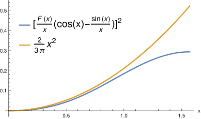
Figure 2: Justifying estimate (5.13).

When using

$$\frac{x}{\sin x}\leq\frac{\pi}{2}\quad\mbox{for all}\;x\in[0,\frac{\pi}{2}],$$

we further have

$$\|w_{h}^{1}\|^{2}_{L^{2}(0,T)} \leq\frac{\pi}{12}\frac{1}{T}\,h^{4}\,\sum\limits_{k=0}^{n-1}\left[\sum\limits_{i=1}^{n}\partial_{t}u(t_{i-1})\,\sin x_{k}\,\sin((2i-1)x_{k})\right]^{2}$$

$$=\frac{\pi}{48}\frac{1}{T}\,h^{4}\,\sum\limits_{k=0}^{n-1}\left[\sum\limits_{i=1}^{n}\partial_{t}u(t_{i-1})\Big{[}\cos(2(i-1)x_{k})-\cos(2ix_{k})\Big{]}\right]^{2}.$$

We write

$$\sum\limits_{i=1}^{n}\partial_{t}u(t_{i-1})\cos(2(i-1)x_{k})=\partial_{t}u(0)+\sum\limits_{i=1}^{n-1}\partial_{t}u(t_{i})\cos(2ix_{k}),$$

while for $i=n$, we have

$$\cos(2nx_{k})=\cos\left(\frac{\pi}{2}+k\pi\right)=0.$$

Hence, we conclude

$$\sum\limits_{i=1}^{n}\partial_{t}u(t_{i-1})\Big{[}\cos(2(i-1)x_{k})-\cos(2ix_{k})\Big{]}\,=\,\partial_{t}u(0)+\sum\limits_{i=1}^{n-1}\Big{[}\partial_{t}u(t_{i})-\partial_{t}u(t_{i-1})\Big{]}\cos(2ix_{k})\,,$$

and using the orthogonality

$$\sum\limits_{k=0}^{n-1}\cos(2ix_{k})\cos(2jx_{k})=\frac{n}{2}\,\delta_{ij},$$

we finally obtain

$$\sum\limits_{k=0}^{n-1} \left[\sum\limits_{i=1}^{n}\partial_{t}u(t_{i-1})\Big{[}\cos(2(i-1)x_{k})-\cos(2ix_{k})\Big{]}\right]^{2}$$

$$= \sum\limits_{k=0}^{n-1}\left[\partial_{t}u(0)+\sum\limits_{i=1}^{n-1}\Big{[}\partial_{t}u(t_{i})-\partial_{t}u(t_{i-1})\Big{]}\cos(2ix_{k})\right]^{2}$$

$$= \sum\limits_{k=0}^{n-1}[\partial_{t}u(0)]^{2}+2\,\partial_{t}u(0)\sum\limits_{i=1}^{n-1}\Big{[}\partial_{t}u(t_{i})-\partial_{t}u(t_{i-1})\Big{]}\sum\limits_{k=0}^{n-1}\cos(2ix_{k})$$

$$+\sum\limits_{i=1}^{n-1}\sum\limits_{j=1}^{n-1}[\partial_{t}u(t_{i})-\partial_{t}u(t_{i-1})][\partial_{t}u(t_{j})-\partial_{t}u(t_{j-1})]\sum\limits_{k=0}^{n-1}\cos(2ix_{k})\cos(2jx_{k})$$

$$= n\,[\partial_{t}u(0)]^{2}+\frac{n}{2}\,\sum\limits_{i=1}^{n-1}[\partial_{t}u(t_{i})-\partial_{t}u(t_{i-1})]^{2}\,\leq\,n\,[\partial_{t}u(0)]^{2}+\frac{n}{2}\,\sum\limits_{i=1}^{n}\left[\int_{t_{i-1}}^{t_{i}}\partial_{tt}u(s)\,ds\right]^{2}$$

$$\leq \,n\,[\partial_{t}u(0)]^{2}+\frac{n}{2}\sum\limits_{i=1}^{n}\int_{t_{i-1}}^{t_{i}}[\partial_{tt}u(s)]^{2}\,ds\int_{t_{i-1}}^{t_{i}}1^{2}\,ds\,=\,n\,[\partial_{t}u(0)]^{2}+\frac{nh}{2}\sum\limits_{i=1}^{n}\int_{t_{i-1}}^{t_{i}}[\partial_{tt}u(s)]^{2}\,ds$$

$$= \,h^{-1}\,T\,[\partial_{t}u(0)]^{2}+\frac{1}{2}\,T\,\int_{0}^{T}[\partial_{tt}u(s)]^{2}\,ds\,.$$

This concludes the proof.  

With the above results, we are in position to give an estimate for $w_{h}=Q_{h}{\mathcal{H}}_{T}^{-1}(u-Q_{h}u)$. When combining (5.7) with (5.8) and (5.12), this gives

$$\|Q_{h}{\mathcal{H}}_{T}^{-1}(u-Q_{h}u)\|_{L^{2}(0,T)}\,\leq\,c\,h^{2}\,\|\partial_{tt}u\|_{L^{2}(0,T)}\,,$$ (5.14)

for $u\in H^{2}(0,T)$ with $\partial_{t}u(0)=0$. For $u\in H^{2}(0,T)$ with $\partial_{t}u(0)\neq 0$, we have to use (5.11) to conclude

$$\|Q_{h}{\mathcal{H}}_{T}^{-1}(u-Q_{h}u)\|_{L^{2}(0,T)}\,\leq\,c\,\Big{[}h^{4}\,\|\partial_{tt}u\|^{2}_{L^{2}(0,T)}+h^{3}\,[\partial_{t}u(0)]^{2}\Big{]}^{1/2}\,.$$ (5.15)

When using a space interpolation argument, we formulate these results in a more general way.

Lemma 5.6

Let $u\in H^{s}_{0,}(0,T):=[H^{2}_{0,}(0,T);H^{1}_{0,}(0,T)]_{s}$ with interpolation norm $\|\cdot\|_{H^{s}_{0,}(0,T)}$ for some $s\in[1,2]$, where the Sobolev space $H^{2}_{0,}(0,T):=\{v\in H^{2}(0,T):v(0)=\partial_{t}v(0)=0\}$ is endowed with the Hilbertian norm $\|\cdot\|_{H^{2}_{0,}(0,T)}:=\|\partial_{tt}(\cdot)\|_{L^{2}(0,T)}$. Then, the estimate

$$\|Q_{h}{\mathcal{H}}_{T}^{-1}(u-Q_{h}u)\|_{L^{2}(0,T)}\,\leq\,c\,h^{s}\,\|u\|_{H^{s}_{0,}(0,T)}$$ (5.16)

holds true.

Proof. For $s=1$ the assertion is (5.4), while for $s=2$, the assertion is (5.14). Then, for $s\in(1,2)$, the assertion follows from a space interpolation argument.  

In order to verify the estimates (5.14) and (5.15), we first consider $u(t)=t^{3}-10t^{2}$, $t\in(0,T)$, $T=2$, with $u\in H^{2}_{0,}(0,T)$, i.e., (5.14) implies second-order convergence, see Table 5 for the numerical results. As a second example, we consider $u(t)=t^{3}-10t$ with $\partial_{t}u(0)=-10$, where (5.15) implies a reduced order of convergence $h^{3/2}$, as observed in the numerical example, see also Table 5.

		$u(t)=t^{3}-10t^{2}$			$u(t)=t^{3}-10t$
$n$		$\|Q_{h}{\mathcal{H}}_{T}^{-1}(u-Q_{h}u)\|_{L^{2}(0,T)}$	eoc		$\|Q_{h}{\mathcal{H}}_{T}^{-1}(u-Q_{h}u)\|_{L^{2}(0,T)}$	eoc
2		1.86270658			1.80230151
4		0.45239154	2.00		0.63072107	1.50
8		0.11030583	2.00		0.21675270	1.50
16		0.02713342	2.00		0.07528792	1.50
32		0.00671882	2.00		0.02637954	1.50
64		0.00167065	2.00		0.00928626	1.50
128		0.00041642	2.00		0.00327641	1.50

Table 5: Numerical results for $\|Q_{h}{\mathcal{H}}_{T}^{-1}(u-Q_{h}u)\|_{L^{2}(0,T)}$ with $T=2$ in the case $u(t)=t^{3}-10t^{2}$ with $\partial_{t}u(0)=0$, and for $u(t)=t^{3}-10t$ with $\partial_{t}u(0)\neq 0$.

When summarizing all previous results, we state the main result of this section.

Theorem 5.7

Assume $u\in H^{s}(0,T)$ for some $s\in[0,1]$. Let $u_{h}\in S_{h}^{0}(0,T)$ be the unique solution of the variational formulation (3.2). Then, the error estimate

$$\|u-u_{h}\|_{L^{2}(0,T)}\leq c\,\left[h^{s}\,\|u\|_{H^{s}(0,T)}+\frac{\|Q_{h}{\mathcal{H}}_{T}^{-1}(u-Q_{h}u)\|_{L^{2}(0,T)}}{c_{S}(u_{h}-Q_{h}u)}\right]$$ (5.17)

holds true $s\in[0,1]$. For $u\in H^{2}(0,T)$ with $\partial_{t}u(0)=0$, we have optimal convergence, i.e.,

$$\|u-u_{h}\|_{L^{2}(0,T)}\leq c\,h\,\|u\|_{H^{2}(0,T)}.$$

With the results of this section, we are in the position to review the numerical examples of Section 3. First, we consider the function $u(t)=\sin(\frac{\pi}{4}t)$ for $t\in(0,2)$. We obviously have $\partial_{t}u(0)\neq 0$, and hence (5.15) applies, i.e., $\|Q_{h}{\mathcal{H}}_{T}^{-1}(u-Q_{h}u)\|_{L^{2}(0,T)}={\mathcal{O}}(h^{3/2})$. On the other hand, we also compute $c_{S}(u_{h}-Q_{h}u)={\mathcal{O}}(h^{1/2})$, see Table 6. In this case, (5.17) gives $\|u-u_{h}\|_{L^{2}(0,T)}={\mathcal{O}}(h)$ as already observed in Table 2.

$n$	$c_{S}(u_{h}-Q_{h}u)$	eoc	$\|Q_{h}\mathcal{H}^{-1}_{T}(u_{h}-Q_{h}u))\|_{L^{2}(0,T)}$	eoc
2	4.290 –1		1.411 –1
4	3.437 –1	0.32	4.922 –2	1.52
8	2.432 –1	0.50	1.691 –2	1.54
16	1.700 –1	0.52	5.888 –3	1.52
32	1.193 –1	0.51	2.067 –3	1.51
64	8.403 –2	0.51	7.284 –4	1.50
128	5.931 –2	0.50	2.572 –4	1.50
256	4.190 –2	0.50	9.086 –5	1.50
512	2.961 –2	0.50	3.211 –5	1.50
1024	2.093 –2	0.50	1.135 –5	1.50
2048	1.480 –2	0.50	4.013 –6	1.50

Table 6: Values of $c_{S}(u_{h}-Q_{h}u)$ and $\|Q_{h}\mathcal{H}^{-1}_{T}(u_{h}-Q_{h}u))\|_{L^{2}(0,T)}$ in the case of a regular function $u(t)=\sin(\frac{\pi}{4}t)$, $t\in(0,2)$.

The second example was the singular function $u(t)=t^{2/3}$, $t\in(0,2)$, i.e., $u\in H^{s}_{0,}(0,T)$ for $s<\frac{7}{6}$. In this case, (5.16) gives $\|Q_{h}{\mathcal{H}}_{T}^{-1}(u-Q_{h}u)\|_{L^{2}(0,T)}={\mathcal{O}}(h^{7/6})$. The numerical results as shown in Table 7 indicate $c_{S}(u_{h}-Q_{h}u)={\mathcal{O}}(h^{1/2})$, and therefore, (5.17) implies $\|u-u_{h}\|_{L^{2}(0,T)}={\mathcal{O}}(h^{2/3})$, as already observed in Table 3.

$n$	$c_{S}(u_{h}-Q_{h}u)$	eoc	$\|Q_{h}\mathcal{H}^{-1}_{T}(u_{h}-Q_{h}u))\|_{L^{2}(0,T)}$	eoc
2	4.467 –1		1.629 –1
4	2.990 –1	0.58	7.255 –2	1.17
8	2.055 –1	0.54	3.233 –2	1.17
16	1.433 –1	0.52	1.440 –2	1.17
32	1.006 –1	0.51	6.415 –3	1.17
64	7.090 –2	0.51	2.858 –3	1.17
128	5.005 –2	0.50	1.273 –3	1.17
256	3.536 –2	0.50	5.670 –4	1.17
512	2.499 –2	0.50	2.526 –4	1.17
1024	1.767 –2	0.50	1.125 –4	1.17
2048	1.249 –2	0.50	5.012 –5	1.17

Table 7: Values of $c_{S}(u_{h}-Q_{h}u)$ and $\|Q_{h}\mathcal{H}^{-1}_{T}(u_{h}-Q_{h}u))\|_{L^{2}(0,T)}$ in the case of the function $u(t)=t^{2/3}$, $t\in(0,2)$, with a singularity at $t=0$.

Finally, we consider the function $u(t)=t(2-t)^{2/3}$, $t\in(0,2)$, with a singularity at the terminate time $T=2$. Again we have $\|Q_{h}{\mathcal{H}}_{T}^{-1}(u-Q_{h}u)\|_{L^{2}(0,T)}={\mathcal{O}}(h^{7/6})$, but in this case we observe, at least asymptotically, $c_{S}(u_{h}-Q_{h}u)={\mathcal{O}}(h^{1/6})$, see Table 8. With these results, (5.17) implies $\|u-u_{h}\|_{L^{2}(0,T)}={\mathcal{O}}(h)$, as already observed in Table 4.

$n$	$c_{S}(u_{h}-Q_{h}u)$	eoc	$\|Q_{h}\mathcal{H}^{-1}_{T}(u_{h}-Q_{h}u))\|_{L^{2}(0,T)}$	eoc
2	4.128 –1		3.040 –1
4	3.391 –1	0.28	1.104 –1	1.46
8	2.599 –1	0.38	3.968 –2	1.48
16	1.952 –1	0.41	1.442 –2	1.46
32	1.476 –1	0.40	5.353 –3	1.43
64	1.138 –1	0.37	2.042 –3	1.39
128	9.009 –2	0.34	8.022 –4	1.35
256	7.326 –2	0.30	3.247 –4	1.31
512	6.106 –2	0.26	1.349 –4	1.27
1024	5.193 –2	0.23	5.724 –5	1.24
2048	4.485 –2	0.21	2.468 –5	1.21

Table 8: Values of $c_{S}(u_{h}-Q_{h}u)$ and $\|Q_{h}\mathcal{H}^{-1}_{T}(u_{h}-Q_{h}u))\|_{L^{2}(0,T)}$ in the case of the function $u(t)=t(2-t)^{2/3}$, $t\in(0,2)$, with a singularity at $T=2$.

6 Conclusions

In this paper, we have given a complete numerical analysis to prove a discrete inf-sup stability condition for the modified Hilbert transformation ${\mathcal{H}}_{T}$. While the stability constant is mesh dependent, related error estimates are still optimal, in most cases. We restrict our theoretical considerations to the case of piecewise constant basis functions, however, this approach can be extended to higher-order basis functions as well, as it is confirmed by numerical results for piecewise linear and second-order basis functions.

These results are of utmost importance in the numerical analysis of space-time finite element methods to analyze discrete inf-sup stability conditions and related error estimates for evolution equations, for both parabolic and hyperbolic problems. In particular, these results will provide the stability and error analysis for a space-time finite element method for the wave equation which is unconditionally stable. While numerical results were already given in [14], its numerical analysis will be given in a forthcoming paper [15]. Further, in the parabolic case, the numerical analysis in [9] of a sparse grid approach based on wavelets also benefits from the results presented here.

Declarations

Conflict of interest: The authors declared that they have no conflict of interest.
Data availability: Data will be made available on request.

Appendix

In this appendix, we provide some of the technical computations which were frequently used within this paper. Let $n\in\mathbb{N}$ be the number of finite elements. First, we recall the definition (4.1) of $x_{k}$. For $k=0,\ldots,2n-1$ and $\mu\in{\mathbb{N}}_{0}$, we consider the shift

$$x_{k+2\mu n}=\left(\frac{\pi}{2}+(k+2\mu n)\pi\right)\frac{1}{2n}=x_{k}+\mu\pi.$$

Then, the evaluation of certain trigonometric functions gives

$$\cos(x_{k+2\mu n}) =\cos(x_{k}+\mu\pi)$$

$$=\cos(x_{k})\,\cos(\mu\pi)-\sin x_{k}\,\sin(\mu\pi)\,=\,(-1)^{\mu}\cos(x_{k}),$$

$$\sin(x_{k+2\mu n}) =\sin(x_{k}+\mu\pi)$$

$$=\sin x_{k}\,\cos(\mu\pi)+\cos(x_{k})\,\sin(\mu\pi)\,=\,(-1)^{\mu}\sin x_{k},$$

$$\sin((2j-1)x_{k+2\mu n}) =\sin[(2j-1)(x_{k}+\mu\pi)]$$

$$=\sin[(2j-1)x_{k}]\cos[(2j-1)\mu\pi]+\cos[(2j-1)x_{k}]\sin[(2j-1)\mu\pi]$$

$$=(-1)^{\mu}\sin[(2j-1)x_{k}],$$

$$\cos((2j-1)x_{k+2\mu n}) =\cos[(2j-1)(x_{k}+\mu\pi)]$$

$$=\cos[(2j-1)x_{k}]\cos[(2j-1)\mu\pi]-\sin[(2j-1)x_{k}]\sin[(2j-1)\mu\pi]$$

$$=(-1)^{\mu}\cos[(2j-1)x_{k}].$$

Next, we consider, for $k=0,\ldots,n-1$,

$$x_{2n-1-k}=\Big{(}\frac{\pi}{2}+(2n-1-k)\pi\Big{)}\frac{1}{2n}=\pi-x_{k},$$

and we compute

$$\cos(x_{2n-1-k}) =\cos(\pi-x_{k})\,=\,-\cos x_{k},$$

$$\sin(x_{2n-1-k}) =\sin(\pi-x_{k})\,=\,\sin x_{k},$$

$$\sin((2j-1)x_{2n-1-k}) =\sin[(2j-1)(\pi-x_{k})]$$

$$=\sin[(2j-1)\pi]\,\cos[(2j-1)x_{k}]-\cos[(2j-1)\pi]\,\sin[(2j-1)x_{k}]$$

$$=\sin[(2j-1)x_{k}],$$

$$\cos((2j-1)x_{2n-1-k}) =\cos[(2j-1)(\pi-x_{k})]$$

$$=\cos[(2j-1)\pi]\,\cos[(2j-1)x_{k}]+\sin[(2j-1)\pi]\,\sin[(2j-1)x_{k}]$$

$$=-\cos[(2j-1)x_{k}].$$

In order to prove (4.2), let us recall [8, Equation 1.342, 4.],

$$\sum\limits_{k=1}^{n}\cos((2k-1)x)=\frac{1}{2}\,\sin(2nx)\,\frac{1}{\cos x},$$

which yields

$$\sum_{i=1}^{n}\cos\left(\Big{(}\frac{\pi}{2}+k\pi\Big{)}\frac{2i-1}{n}\right)=\frac{1}{2}\,\sin\Big{(}(2k+1)\pi\Big{)}\frac{1}{\cos\left(\Big{(}\frac{\pi}{2}+k\pi\Big{)}\frac{1}{n}\right)}\,=\,0.$$

For the computation of the Fourier coefficients (4.4), we consider

$$\overline{u}_{k} =\frac{2}{T}\int_{0}^{T}u_{h}(t)\,\cos\left(\Big{(}\frac{\pi}{2}+k\pi\Big{)}\frac{t}{T}\right)\,dt$$

$$=\frac{2}{T}\sum\limits_{i=1}^{n}u_{i}\int_{t_{i-1}}^{t_{i}}\cos\left(\Big{(}\frac{\pi}{2}+k\pi\Big{)}\frac{t}{T}\right)\,dt$$

$$=\frac{2}{T}\sum\limits_{i=1}^{n}u_{i}\frac{T}{\frac{\pi}{2}+k\pi}\left[\sin\left(\Big{(}\frac{\pi}{2}+k\pi\Big{)}\frac{t}{T}\right)\right]_{t_{i-1}}^{t_{i}}$$

$$=\frac{2}{\frac{\pi}{2}+k\pi}\sum\limits_{i=1}^{n}u_{i}\left[\sin\left(\Big{(}\frac{\pi}{2}+k\pi\Big{)}\frac{t_{i}}{T}\right)-\sin\left(\Big{(}\frac{\pi}{2}+k\pi\Big{)}\frac{t_{i-1}}{T}\right)\right]$$

and further,

$$\overline{u}_{k} =\frac{4}{\frac{\pi}{2}+k\pi}\sum\limits_{i=1}^{n}u_{i}\cos\left(\Big{(}\frac{\pi}{2}+k\pi\Big{)}\frac{t_{i}+t_{i-1}}{2T}\right)\sin\left(\Big{(}\frac{\pi}{2}+k\pi\Big{)}\frac{t_{i}-t_{i-1}}{2T}\right)$$

$$=4\frac{\sin\left(\Big{(}\frac{\pi}{2}+k\pi\Big{)}\frac{h}{2T}\right)}{\frac{\pi}{2}+k\pi}\sum\limits_{i=1}^{n}u_{i}\cos\left(\Big{(}\frac{\pi}{2}+k\pi\Big{)}\frac{2i-1}{2n}\right)$$

$$=\frac{2}{n}\,\frac{\sin\left(\Big{(}\frac{\pi}{2}+k\pi\Big{)}\frac{1}{2n}\right)}{(\frac{\pi}{2}+k\pi)\frac{1}{2n}}\sum\limits_{i=1}^{n}u_{i}\cos\left(\Big{(}\frac{\pi}{2}+k\pi\Big{)}\frac{2i-1}{2n}\right)$$

$$=\frac{2}{n}\,\frac{\sin x_{k}}{x_{k}}\,\sum\limits_{i=1}^{n}u_{i}\cos((2i-1)x_{k}).$$

In particular for $k=0,\ldots,2n-1$ and $\mu\in{\mathbb{N}}_{0}$, we then conclude (4.5) from

$$\overline{u}_{k+2\mu n} =\frac{2}{n}\,\frac{\sin(x_{k+2\mu n})}{x_{k+2\mu n}}\,\sum\limits_{i=1}^{n}u_{i}\,\cos((2i-1)x_{k+2\mu n})$$

$$=\frac{2}{n}\,\frac{(-1)^{\mu}\sin x_{k}}{x_{k+2\mu n}}\,\sum\limits_{i=1}^{n}u_{i}\,(-1)^{\mu}\cos((2i-1)x_{k})$$

$$=\frac{x_{k}}{x_{k+2\mu n}}\,\frac{2}{n}\,\frac{\sin x_{k}}{x_{k}}\,\sum\limits_{i=1}^{n}u_{i}\,\cos((2i-1)x_{k})\,=\,\frac{2k+1}{2k+1+4\mu n}\,\overline{u}_{k}.$$

Next, for $k=0,1,\ldots,n-1$, we calculate that

$$\overline{u}_{2n-1-k} =\frac{2}{n}\,\frac{\sin(x_{2n-1-k})}{x_{2n-1-k}}\,\sum\limits_{i=1}^{n}u_{i}\,\cos((2i-1)x_{2n-1-k})$$

$$=-\frac{2}{n}\,\frac{\sin x_{k}}{x_{2n-1-k}}\,\sum\limits_{i=1}^{n}u_{i}\,\cos((2i-1)x_{k})$$

$$=-\frac{x_{k}}{x_{2n-1-k}}\,\frac{2}{n}\,\frac{\sin x_{k}}{x_{k}}\,\sum\limits_{i=1}^{n}u_{i}\,\cos((2i-1)x_{k})\,=\,-\frac{2k+1}{4n-1-2k}\,\overline{u}_{k}^{1},$$

i.e., (4.6) follows.

For the determination of the coefficients (4.12), we compute that

$$w_{j} =\frac{1}{h}\int_{t_{j-1}}^{t_{j}}({\mathcal{H}}_{T}^{-1}u_{h})(t)\,dt$$

$$=\frac{1}{h}\sum\limits_{k=0}^{\infty}\overline{u}_{k}\int_{t_{j-1}}^{t_{j}}\sin\left(\Big{(}\frac{\pi}{2}+k\pi\Big{)}\frac{t}{T}\right)\,dt$$

$$=\frac{1}{h}\sum\limits_{k=0}^{\infty}\overline{u}_{k}\frac{T}{\frac{\pi}{2}+k\pi}\left[-\cos\left(\Big{(}\frac{\pi}{2}+k\pi\Big{)}\frac{t}{T}\right)\right]_{t_{j-1}}^{t_{j}}$$

$$=\frac{1}{h}\sum\limits_{k=0}^{\infty}\overline{u}_{k}\frac{T}{\frac{\pi}{2}+k\pi}\left[\cos\left(\Big{(}\frac{\pi}{2}+k\pi\Big{)}\frac{t_{j-1}}{T}\right)-\cos\left(\Big{(}\frac{\pi}{2}+k\pi\Big{)}\frac{t_{j}}{T}\right)\right]$$

and further,

$$w_{j} =\frac{1}{h}\sum\limits_{k=0}^{\infty}\overline{u}_{k}\frac{2T}{\frac{\pi}{2}+k\pi}\sin\left(\Big{(}\frac{\pi}{2}+k\pi\Big{)}\frac{t_{j}+t_{j-1}}{2T}\right)\sin\left(\Big{(}\frac{\pi}{2}+k\pi\Big{)}\frac{t_{j}-t_{j-1}}{2T}\right)$$

$$=\frac{1}{h}\sum\limits_{k=0}^{\infty}\overline{u}_{k}\frac{2T}{\frac{\pi}{2}+k\pi}\sin\left(\Big{(}\frac{\pi}{2}+k\pi\Big{)}\frac{2j-1}{2n}\right)\sin\left(\Big{(}\frac{\pi}{2}+k\pi\Big{)}\frac{h}{2T}\right)$$

$$=\sum\limits_{k=0}^{\infty}\overline{u}_{k}\frac{\sin\left(\Big{(}\frac{\pi}{2}+k\pi\Big{)}\frac{h}{2T}\right)}{(\frac{\pi}{2}+k\pi)\frac{h}{2T}}\sin\left(\Big{(}\frac{\pi}{2}+k\pi\Big{)}\frac{2j-1}{2n}\right)$$

$$=\sum\limits_{k=0}^{\infty}\overline{u}_{k}\,\frac{\sin x_{k}}{x_{k}}\,\sin((2j-1)x_{k}).$$

To prove (4.13), we have

$$w_{j} =\sum\limits_{k=0}^{\infty}\overline{u}_{k}\,\frac{\sin x_{k}}{x_{k}}\,\sin((2j-1)x_{k})$$

$$=\sum\limits_{k=0}^{2n-1}\sum\limits_{\mu=0}^{\infty}\overline{u}_{k+2\mu n}\,\frac{\sin(x_{k+2\mu n})}{x_{k+2\mu n}}\,\sin((2j-1)x_{k+2\mu n})$$

$$=\sum\limits_{k=0}^{2n-1}\sum\limits_{\mu=0}^{\infty}\overline{u}_{k+2\mu n}\,\frac{(-1)^{\mu}\sin x_{k}}{x_{k+2\mu n}}\,(-1)^{\mu}\sin((2j-1)x_{k})$$

$$=\sum\limits_{k=0}^{2n-1}\overline{u}_{k}\left(\sum\limits_{\mu=0}^{\infty}\frac{(2k+1)^{2}}{(2k+1+4\mu n)^{2}}\right)\,\frac{\sin x_{k}}{x_{k}}\,\sin((2j-1)x_{k})$$

$$=\sum\limits_{k=0}^{2n-1}\overline{u}_{k}\,\gamma(k,n)\,\frac{\sin x_{k}}{x_{k}}\,\sin((2j-1)x_{k})$$

when using (4.5).

Next, we use (4.6) to conclude from (4.13) that

$$w_{j}= \sum\limits_{k=0}^{2n-1}\overline{u}_{k}\,\gamma(k,n)\,\frac{\sin x_{k}}{x_{k}}\,\sin((2j-1)x_{k})$$

$$= \sum\limits_{k=0}^{n-1}\left[\overline{u}_{k}\,\gamma(k,n)\,\frac{\sin x_{k}}{x_{k}}\sin((2j-1)x_{k})\right.$$

$$\left.+\overline{u}_{2n-1-k}\,\gamma(2n-1-k,n)\,\frac{\sin(x_{2n-1-k})}{x_{2n-1-k}}\,\sin((2j-1)x_{2n-1-k})\right]$$

$$= \sum\limits_{k=0}^{n-1}\overline{u}_{k}\Big{[}\gamma(k,n)-\gamma(2n-1-k,n)\frac{(2k+1)^{2}}{(4n-1-2k)^{2}}\Big{]}\frac{\sin x_{k}}{x_{k}}\,\sin((2j-1)x_{k}),$$

which yields (4.14).

References

[1]
P. Auscher, M. Egert, K. Nyström: well-posedness of boundary
value problems for parabolic systems with measurable coefficients.
J. Eur. Math. Soc. 22 (2020) 2943–3058.
[2]
I. Babuška, R. Narasimhan: The Babušla–Brezzi condition and the
patch test: an example.
Comput. Methods Appl. Mech. Engrg. 140 (1997) 183–199.
[3]
F. Bertrand, D. Boffi:
On the necessity of the inf-sup condition for a mixed finite
element formulation. IMA J. Numer. Anal., to appear, 2024.
[4]
P. L. Butzer, W. Trebels: Hilbert Transformation, gebrochene
Integration und Differentiation. Springer Fachmedien, Wiesbaden, 1968.
[5]
D. Devaud: Petrov–Galerkin space-time -approximation of parabolic equations in .
IMA J. Numer. Anal. 40 (2020) 2717–2745.
[6]
M. Ferrari: Some properties of a modified Hilbert transform.
Preprint, 2023.
[7]
M. Fontes: Parabolic equations with low regularity.
Ph.D. Thesis, Department of Mathematics, Lund
Institute of Technology, Lund, 1996.
[8]
I. S. Gradshteyn, I. M. Ryzhik: Table of integrals, series, and products.
Amsterdam: Elsevier/Academic Press, 2015.
[9]
H. Harbrecht, C. Schwab, M. Zank:
Wavelet compressed, modified Hilbert transformation
in space-time discretization of the heat equation, in preparation, 2024.
[10]
J. I. M. Hauser, M. Zank: Numerical study of conforming space-time
methods for Maxwell’s equations. Numer. Methods Partial Differ. Eq.
40 (2024) e23070.
[11]
F. W. King: Hilbert Transforms. Encyclopedia of Mathematics and its Applications, vol. 1, Cambridge University Press, 2009.
[12]
U. Langer, M. Zank: Efficient direct space-time finite element solvers
for parabolic initial-boundary value problems in anisotropic Sobolev
spaces. SIAM J. Sci. Comput. 43 (2021) A2714–A2736.
[13]
S. Larsson, C. Schwab: Compressive space-time Galerkin discretizations
of parabolic partial differential equations.
arXiv:1501.04514v1, 2015.
[14]
R. Löscher, O. Steinbach, M. Zank: Numerical results for an
unconditionally stable space-time finite element method for the
wave equation. In: Domain Decomposition Methods in Science and
Engineering XXVI (S. Brenner, E. Chung, A. Klawonn, F. Kwok, J. Xu,
J. Zou eds.). Lecture Notes in Computational Science and Engineering,
vol. 145, Springer, Cham, pp. 625–632, 2022.
[15]
R. Löscher, O. Steinbach, M. Zank:
An unconditionally stable space-time finite element
method for the wave equation, in preparation, 2024.
[16]
I. Perugia, C. Schwab, M. Zank: Exponential convergence of
-time-stepping in space-time discretizations of parabolic PDES.
ESAIM Math. Model. Numer. Anal. 57 (2023) 29–67.
[17]
O. Steinbach: Numerical Approximation Methods for Elliptic Boundary
Value Problems. Finite and Boundary Elements. Springer, New York, 2008.
[18]
O. Steinbach, A. Missoni: A note on a modified Hilbert transform.
Appl. Anal. 102 (2023) 2583–2590.
[19]
O. Steinbach, C. Urzua–Torres, M. Zank: Towards coercive boundary
element methods for the wave equation.
J. Integral Equations Appl. 34 (2022) 501–515.
[20]
O. Steinbach, M. Zank: Coercive space-time finite element methods
for initial boundary value problems.
Electron. Trans. Numer. Anal. 52 (2020) 154–194.
[21]
O. Steinbach, M. Zank: A note on the efficient evaluation of a
modified Hilbert transformation. J. Numer. Math. 29 (2021) 47–61.
[22]
F. Stummel: The generalized patch test.
SIAM J. Numer. Anal. 16 (1979) 449–471.
[23]
F. Stummel: The limitations of the test patch.
Internat. J. Numer. Methods Engrg. 15 (1980) 177–188.
[24]
J. Xu, L. Zikatanov: Some observations on Babuška and
Brezzi theories. Numer. Math. 94 (2003) 195–202.
[25]
M. Zank: Inf-sup stable space-time methods for time-dependent partial
differential equations, Monographic Series TU Graz/Computation in
Engineering and Science, vol. 36, Verlag der Technischen
Universität Graz, Graz, 2020.
[26]
M. Zank: An exact realization of a modified Hilbert transformation for space-time methods for parabolic evolution equations.
Comput. Methods Appl. Math. 21 (2021), no. 2, 479–496.
[27]
M. Zank: Integral Representations and quadrature schemes for the modified Hilbert transformation.
Comput. Methods Appl. Math. 23 (2023), no. 2, 473–489.
[28]
O. C. Zienkiewicz, R. L. Taylor: The finite element patch test revisted.
A computer test for convergence, validation and error estimates.
Comput. Methods Appl. Mech. Engrg. 149 (1997) 223–254.