Theoretical properties of angular halfspace depth

Abstract.

The angular halfspace depth (ahD) is a natural modification of the celebrated halfspace (or Tukey) depth to the setup of directional data. It allows us to define elements of nonparametric inference, such as the median, the inter-quantile regions, or the rank statistics, for datasets supported in the unit sphere. Despite being introduced in 1987, ahD has never received ample recognition in the literature, mainly due to the lack of efficient algorithms for its computation. With the recent progress on the computational front, ahD however exhibits the potential for developing viable nonparametric statistics techniques for directional datasets. In this paper, we thoroughly treat the theoretical properties of ahD. We show that similarly to the classical halfspace depth for multivariate data, also ahD satisfies many desirable properties of a statistical depth function. Further, we derive uniform continuity/consistency results for the associated set of directional medians, and the central regions of ahD, the latter representing a depth-based analogue of the quantiles for directional data.

1. Nonparametrics of directional data and angular halfspace depth

Directional data analysis concerns the statistics of datasets bound to lie on the unit sphere $\mathbb{S}^{d-1}=\left\{x\in\mathbb{R}^{d}\colon\left\|x\right\|=1\right\}$. Despite sharing similarities with multivariate statistical methods, the particular geometry of the sphere makes the analysis of directional data challenging. The sphere $\mathbb{S}^{d-1}$ is a symmetric compact manifold, which makes many statistical methods from $\mathbb{R}^{d}$ fruitless or suboptimal when applied in $\mathbb{S}^{d-1}$ directly (Watson,, 1983, Mardia and Jupp,, 2000, Ley and Verdebout,, 2017).

We consider the nonparametric analysis for directional data and the concept of depth functions, a statistical tool that introduces elements of nonparametrics to multivariate or non-Euclidean spaces. In the past decades, depths have garnered great success in multivariate analysis (Donoho and Gasko,, 1992, Liu et al.,, 1999, Zuo and Serfling,, 2000, Mosler,, 2013, Chernozhukov et al.,, 2017, Mosler and Mozharovskyi,, 2022). A prime example of a depth in the Euclidean space $\mathbb{R}^{d}$ is the halfspace depth (hD, also called Tukey depth, or location depth) that is defined for $x\in\mathbb{R}^{d}$ and a Borel probability measure $P$ on $\mathbb{R}^{d}$ by

(1) $$hD(x;P)=\inf\left\{P\left(H_{x,u}\right)\colon u\in\mathbb{S}^{d-1}\right\},$$

where $H_{x,u}=\left\{y\in\mathbb{R}^{d}\colon\left\langle y,u\right\rangle\geq\left\langle x,u\right\rangle\right\}$ is the closed halfspace whose boundary passes through $x$ with inner unit normal $u$. In words, hD evaluates the smallest $P$-mass of a halfspace that contains $x$. As such, it allows to devise a $P$-dependent ordering of the points from $\mathbb{R}^{d}$ — a point $x$ is said to be located deeper than $y$ inside the mass of $P$ if $hD(x;P)>hD(y;P)$. The deepest point in $\mathbb{R}^{d}$, defined as (any) point that maximizes the depth function $x\mapsto hD(x;P)$ over $\mathbb{R}^{d}$, is a natural analogue of the median for $\mathbb{R}^{d}$-valued measures and is called a halfspace median of $P$. A counterpart of quantiles (or, more precisely, inter-quantile regions) in $\mathbb{R}^{d}$ are the central regions of $P$, given as the upper level sets of hD

(2) $$hD_{\alpha}(P)=\left\{x\in\mathbb{R}^{d}\colon hD(x;P)\geq\alpha\right\}\quad\mbox{for }\alpha\geq 0.$$

These sets are known to be nested, convex, and compact for $\alpha>0$; their shapes capture the geometry of $P$. Both the multivariate medians and central regions are of great importance in nonparametric analysis of multivariate data, and have been studied extensively in the literature (Donoho and Gasko,, 1992, Rousseeuw and Ruts,, 1999, Zuo and Serfling,, 2000, Dyckerhoff,, 2017). The halfspace depth is only one of many depth functions proposed in multivariate analysis. It is, nevertheless, the classical representative of multivariate depths.

Several depths suitable specifically for directional data have been proposed in the literature; we refer to Liu and Singh, (1992), Agostinelli and Romanazzi, (2013), Ley et al., (2014), Pandolfo et al., (2018), Buttarazzi et al., (2018), Konen, (2022), and Hallin et al., (2022). In this contribution, we scrutinize historically the first directional depth function proposed by Small, (1987, Example 2.3.4). It is a version of hD from (1) suitable for measures in $\mathbb{S}^{d-1}$. For $x\in\mathbb{S}^{d-1}$ and $P$ a Borel probability measure on $\mathbb{S}^{d-1}$, the angular halfspace depth (ahD, also known as angular Tukey depth) of $x$ with respect to (w.r.t.) $P$ is defined as

(3) $$ahD\left(x;P\right)=\inf\left\{P\left(H_{0,u}\right)\colon u\in\mathbb{S}^{d-1}\mbox{ and }x\in H_{0,u}\right\}.$$

In contrast to the standard hD in (1), in the definition of ahD one considers only halfspaces whose boundary passes through the origin $0$ in the ambient space $\mathbb{R}^{d}$, and searches for a minimum $P$-mass among those that contain $x$.

The first rigorous studies of ahD were conducted by Small, (1987) and Liu and Singh, (1992, Section 4). Since then, no systematic investigation of the theory of ahD has been performed. In fact, it might come as a surprise how little attention did ahD receive in the literature, especially when compared with the abundant body of research on the classical hD. One explanation for this is the presumed high computational cost of the angular depth, coupled with a lack of efficient algorithms for its computation (Pandolfo et al.,, 2018). The problem of exact and approximate computation of ahD was, however, recently resolved in Dyckerhoff and Nagy, (2023), which paved the way to explore the general theory and practice of ahD with its statistical applications.

This paper comprehensively studies the main theoretical properties of ahD, its associated median, and its central regions. We contrast ahD with hD and demonstrate that similarly to the halfspace depth in $\mathbb{R}^{d}$, also the angular depth satisfies an array of plausible properties required from a proper depth function. After introducing the notations, we begin in Section 2 by drawing a direct relation between ahD on the sphere $\mathbb{S}^{d-1}$ and a variant of hD in $\mathbb{R}^{d-1}$. Then, in Section 3, we study ahD w.r.t. the desirable properties of a directional depth formulated recently in Nagy et al., (2023). We show that ahD, as the only directional depth function found in the literature, satisfies all the conditions from Nagy et al., (2023). In the final Section 4 we provide a list of additional characteristics of ahD, mainly related to the continuity of its median and the associated central regions. Those findings are important in statistical practice, as they guarantee the uniform consistency of the sample depth (3) when computed w.r.t. the empirical measure of a random sample $X_{1},\dots,X_{n}$ from distribution $P$. The proofs of all theoretical results are gathered in the Appendix.

Notations

We write $e_{j}\in\mathbb{S}^{d-1}$ for the $j$-th canonical vector in $\mathbb{R}^{d}$, $j=1,\dots,d$. That is, $e_{1}=(1,0,\dots,0)^{\mathsf{T}}$ etc. We denote by $\mathcal{H}=\left\{H_{x,u}\colon x\in\mathbb{R}^{d}\mbox{ and }u\in\mathbb{S}^{d-1}\right\}$ the collection of all halfspaces in $\mathbb{R}^{d}$, and by $\mathcal{H}_{0}=\left\{H_{0,u}\in\mathcal{H}\colon u\in\mathbb{S}^{d-1}\right\}$ those halfspaces in $\mathbb{R}^{d}$ whose boundary passes through the origin. For a set $A\subset\mathbb{R}^{d}$, we write $A^{\circ}$ for the interior of $A$ and $\partial A$ for the topological boundary of $A$. Sometimes we use $A^{\circ}$ ($\partial A$) to denote the relative interior (boundary) of $A$, that is the interior (boundary) considered in the smallest affine subspace containing $A$. Whether we consider relative interior (boundary) or not will always be clear from the context. The complement of $A$ is $A^{\mathsf{c}}$. A set $A\subseteq\mathbb{S}^{d-1}$ is called spherical convex (see, e.g., Besau and Werner,, 2016) if its radial extension defined as $\mathrm{rad}\left(A\right)=\left\{\lambda\,a\in\mathbb{R}^{d}\colon a\in A\mbox{ and }\lambda>0\right\}$ is convex in $\mathbb{R}^{d}$. We denote by $\mathbb{S}^{d-1}_{+}=\left\{y\in\mathbb{S}^{d-1}\colon\left\langle y,e_{d}\right\rangle>0\right\}$ and $\mathbb{S}^{d-1}_{-}=\left\{y\in\mathbb{S}^{d-1}\colon\left\langle y,e_{d}\right\rangle<0\right\}$ the (open) “northern” hemisphere with a pole at $e_{d}$, and the (open) “southern” hemisphere centered at $-e_{d}$, respectively. The set $\mathbb{S}^{d-1}_{0}=\left\{y\in\mathbb{S}^{d-1}\colon\left\langle y,e_{d}\right\rangle=0\right\}$ is called the “equator” of the $(d-1)$-sphere $\mathbb{S}^{d-1}$.

Let $\left(\Omega,\mathcal{A},\mathsf{P}\right)$ be the probability space on which all random variables are defined. For a topological space $\mathcal{X}$, $\mathcal{P}\left({\mathcal{X}}\right)$ stands for the collection of all Borel probability measures on $\mathcal{X}$, and $X\sim P\in\mathcal{P}\left({\mathcal{X}}\right)$ means that $X$ is a random variable in $\mathcal{X}$ with distribution $P$. For $\varphi\colon\mathcal{X}\to\mathcal{Y}$ a map between topological spaces, we write $P_{\varphi(X)}\in\mathcal{P}\left({\mathcal{Y}}\right)$ for the distribution of $\varphi(X)$ with $X\sim P\in\mathcal{P}\left({\mathcal{X}}\right)$. Further, $\mathcal{M}\left(\mathcal{X}\right)$ represents the collection of all finite Borel measures on $\mathcal{X}$. Certainly, $\mathcal{P}\left({\mathcal{X}}\right)\subset\mathcal{M}\left(\mathcal{X}\right)$. Weak convergence of a sequence of measures $\left\{P_{n}\right\}_{n=1}^{\infty}\subset\mathcal{M}\left(\mathcal{X}\right)$ to $P\in\mathcal{M}\left(\mathcal{X}\right)$ is denoted by $P_{n}\xrightarrow{w}P$ as $n\to\infty$. Finally, we say that $Q$ is a (finite Borel) signed measure on a topological space $\mathcal{X}$ if there exist two finite Borel measures $Q_{+},Q_{-}\in\mathcal{M}\left(\mathcal{X}\right)$ such that (Dudley,, 2002, Theorem 5.6.1)

(4) $$Q(B)=Q_{+}(B)-Q_{-}(B)\quad\mbox{for all $B\subseteq\mathcal{X}$ Borel}.$$

A signed measure can attain both positive and negative values. We denote by $\mathcal{S}\left({\mathcal{X}}\right)$ the set of all finite Borel signed measures on $\mathcal{X}$, and note that $\mathcal{M}\left(\mathcal{X}\right)\subset\mathcal{S}\left({\mathcal{X}}\right)$.

2. Gnomonic projection and $ahD$

We begin our study by drawing connections of ahD in $\mathbb{S}^{d-1}$ with the standard (Euclidean) hD in $\mathbb{R}^{d-1}$. They will allow us to use the abundance of theoretical results available for hD and adapt them to the setup of directional measures. First, note that the halfspace depth (1) is well defined not only for probability measures but for any (finite) Borel measures $P\in\mathcal{M}\left(\mathbb{R}^{d}\right)$. It can be written in two equivalent forms, either as

(5) $$hD\left(x;P\right)=\inf\left\{P\left(H\right)\colon H\in\mathcal{H}\mbox{ and }x\in H\right\},$$

or also as

(6) $$hD\left(x;P\right)=\inf\left\{P\left(H\right)\colon H\in\mathcal{H}\mbox{ and }x\in\partial H\right\}.$$

In what follows, we employ the halfspace depth with signed measures. In case when $Q\in\mathcal{S}\left({\mathbb{R}^{d}}\right)$ can attain negative values, the two definitions of hD in (5) and (6) differ; a halfspace $H$ containing $x$ in its interior may have strictly smaller $Q$-mass than its subset $H^{\prime}$ with $x\in\partial H^{\prime}$. Out of the two possibilities of defining hD for signed measures, it will be convenient to use the first one in (5). We say that the halfspace depth of $x\in\mathbb{R}^{d}$ w.r.t. $Q\in\mathcal{S}\left({\mathbb{R}^{d}}\right)$ is defined as

(7) $$hD\left(x;Q\right)=\inf\left\{Q\left(H\right)\colon H\in\mathcal{H}\mbox{ and }x\in H\right\}.$$

We use the same notation for both halfspace depth of measures from $\mathcal{M}\left(\mathbb{R}^{d}\right)$ and signed measures from $\mathcal{S}\left({\mathbb{R}^{d}}\right)$; the standard depth (5) is only a particular case of our more general depth (7).

Our task is to express ahD of $x\in\mathbb{S}^{d-1}$ w.r.t. $P\in\mathcal{P}\left({\mathbb{S}^{d-1}}\right)$. Throughout this section, we make the following assumption on $P$ and $x$

(8) $$P(\mathbb{S}^{d-1}_{0})=0\quad\mbox{and}\quad x\in\mathbb{S}^{d-1}_{+}.$$

This assumption is made without loss of generality due to the rotational invariance of ahD that will be formally proved as Theorem 2 in Section 3.1. Denote by $\mathcal{G}=\left\{y\in\mathbb{R}^{d}\colon\left\langle y,e_{d}\right\rangle=1\right\}$ the hyperplane tangent to $\mathbb{S}^{d-1}$ at the pole $e_{d}\in\mathbb{R}^{d}$, see Figure 1. Consider the mapping

(9) $$\xi\colon\mathbb{S}^{d-1}\setminus\mathbb{S}^{d-1}_{0}\to\mathcal{G}\colon x\mapsto x/\left\langle x,e_{d}\right\rangle$$

that takes points $x\in\mathbb{S}^{d-1}$ not on the equator to the unique point of $\mathcal{G}$ on the straight line between $x$ and the origin. This map is visualized for $d=2$ and $d=3$ in Figure 1. In what follows, we will canonically identify the hyperplane $\mathcal{G}$ with $\mathbb{R}^{d-1}$ by formally dropping the last coordinate $\left\langle y,e_{d}\right\rangle=1$ of points $y\in\mathcal{G}$. This allows us to write also $\xi(x)\in\mathbb{R}^{d-1}$ for any $x\in\mathbb{S}^{d-1}\setminus\mathbb{S}^{d-1}_{0}$. The map (9) is called the gnomonic projection of the sphere $\mathbb{S}^{d-1}$ into $\mathcal{G}$ (or $\mathbb{R}^{d-1}$, see Besau and Werner,, 2016). It is a double covering of $\mathbb{R}^{d-1}$, once for points from $\mathbb{S}^{d-1}_{+}$ and once for those from $\mathbb{S}^{d-1}_{-}$. On $\mathbb{S}^{d-1}_{+}$ (or $\mathbb{S}^{d-1}_{-}$) it is a bijection with $\mathbb{R}^{d-1}$. The points from the equator $\mathbb{S}^{d-1}_{0}$ are not considered in (9). This will not be a problem because of our assumption (8).

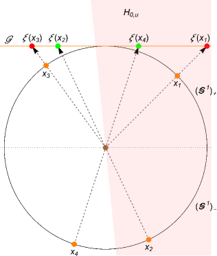
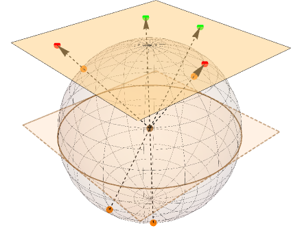
Figure 1. Transformation $\xi$ that takes $\mathbb{S}^{d-1}\setminus\mathbb{S}^{d-1}_{0}$ to $\mathcal{G}$ for $d=2$ (left panel) and $d=3$ (right panel). The data from the northern hemisphere $\mathbb{S}^{d-1}_{+}$ are mapped into points of positive $P_{\pm}$-mass in $\mathcal{G}$ (red points), while data from the southern hemisphere $\mathbb{S}^{d-1}_{-}$ project to points of negative $P_{\pm}$-mass (green points). In the left panel we see also a halfspace $H_{0,u}\in\mathcal{H}_{0}$ (shaded halfplane). Only points $x_{1}\in\mathbb{S}^{1}_{+}$ and $x_{2}\in\mathbb{S}^{1}_{-}$ lie in $H_{0,u}$, which means that precisely $\xi(x_{1})$ and $\xi(x_{4})$ are contained in $G_{u}=H_{0,u}\cap\mathcal{G}$. This is in accordance with formula (30).

Denote for any $B\subseteq\mathcal{G}$ (or $B\subseteq\mathbb{R}^{d-1}$) Borel

$$P_{+}(B) =P\left(\left\{y\in\mathbb{S}^{d-1}_{+}\colon\xi(y)\in B\right\}\right), P_{-}(B) =P\left(\left\{y\in\mathbb{S}^{d-1}_{-}\colon\xi(y)\in B\right\}\right),$$

the pushforward measures of restrictions of $P$ to $\mathbb{S}^{d-1}_{+}$ and $\mathbb{S}^{d-1}_{-}$, respectively, under the gnomonic projection $\xi$. In words, $P_{+}$ is the image measure of the part of $P$ in the northern hemisphere when projected to $\mathcal{G}$ (or $\mathbb{R}^{d-1}$), and $P_{-}$ analogously for the southern hemisphere. We patch $P_{+}$ and $P_{-}$ together and use them to define a signed measure $P_{\pm}\in\mathcal{S}\left({\mathbb{R}^{d-1}}\right)$ given by (4)

(10) $$P_{\pm}(B)=P\left(\left\{x\in\mathbb{S}^{d-1}_{+}\colon\xi(x)\in B\right\}\right)-P\left(\left\{x\in\mathbb{S}^{d-1}_{-}\colon\xi(x)\in B\right\}\right)\quad\mbox{for $B\subseteq\mathbb{R}^{d-1}$ Borel}.$$

The signed measure $P_{\pm}$ takes a simple form when $P$ is an empirical measure of $n$ data points $x_{1},\dots,x_{n}\in\mathbb{S}^{d-1}$. In that situation, $P_{\pm}$ is simply a signed empirical measure, with atoms of positive mass $1/n$ at each $\xi(x_{i})$ such that $x_{i}\in\mathbb{S}^{d-1}_{+}$, and atoms of negative mass $-1/n$ at $\xi(x_{i})$ for $x_{i}\in\mathbb{S}^{d-1}_{-}$. In this situation, the gnomonic projection was essential to design fast computational algorithms for the sample ahD in Dyckerhoff and Nagy, (2023).

Our principal tool for analyzing ahD is its relation with hD, which is described in the following theorem. In that result, we say that a set $H$ is called a generalized halfspace in $\mathbb{R}^{d-1}$ if $H$ is a halfspace in $\mathbb{R}^{d-1}$, an empty set, or the whole space $\mathbb{R}^{d-1}$ itself.

Theorem 1.

Let $P\in\mathcal{P}\left({\mathbb{S}^{d-1}}\right)$ and $x\in\mathbb{S}^{d-1}$ be such that (8) is true. Then

(11) $$ahD(x;P)=P\left(\mathbb{S}^{d-1}_{-}\right)+\inf\left\{P_{+}\left(H\right)-P_{-}\left(H^{\circ}\right)\colon H\in\mathcal{H}^{*}\mbox{ and }\xi(x)\in H\right\}$$

for $\mathcal{H}^{*}$ the set of all generalized halfspaces in $\mathbb{R}^{d-1}$. If, in addition,

(12) $$P\left(\partial H\cap\mathbb{S}^{d-1}_{-}\right)=0\quad\mbox{for all }H\in\mathcal{H}_{0},$$

then

$$ahD(x;P)=P(\mathbb{S}^{d-1}_{-})+hD(\xi(x);P_{\pm}).$$

Formula (11) will be quite useful in deriving theoretical properties of ahD and constructing examples, as we will see throughout this paper.

3. Desiderata for a directional depth function

There are several well-established properties that a depth $D$ in a linear space $\mathbb{R}^{d}$ should obey. It is typically agreed that $D$ should be • affine invariant, meaning that it does not depend on the coordinate system in $\mathbb{R}^{d}$; • maximized at the center of symmetry of $P$ for any $P\in\mathcal{P}\left({\mathbb{R}^{d}}\right)$ symmetric; • monotonically decreasing as $x$ moves along straight lines starting at the point of maximum of $D$; and • decaying uniformly to zero as $\left\|x\right\|\to\infty$. This set of properties was postulated by Zuo and Serfling, (2000); for additional related axioms we refer to Liu, (1990), Serfling, (2006), Mosler, (2013), and Mosler and Mozharovskyi, (2022).

Compared to depths in $\mathbb{R}^{d}$, much less is known about general depth functions defined in $\mathbb{S}^{d-1}$. One set of assumptions has been laid down recently in Nagy et al., (2023). There, a general angular (or directional) depth function $aD$ was introduced as a bounded map $aD\colon\mathbb{S}^{d-1}\times\mathcal{P}\left({\mathbb{S}^{d-1}}\right)\to[0,\infty)$ that fulfills (most of) the following properties for all $P\in\mathcal{P}\left({\mathbb{S}^{d-1}}\right)$:

1. Rotational invariance: $aD(x;P)=aD(Ox;P_{OX})$ for all $x\in\mathbb{S}^{d-1}$ and any orthogonal matrix $O\in\mathbb{R}^{d\times d}$, where $P_{OX}\in\mathcal{P}\left({\mathbb{S}^{d-1}}\right)$ is the distribution of the transformed random vector $OX$ with $X\sim P$;

2. Maximality at center: For any $P\in\mathcal{P}\left({\mathbb{S}^{d-1}}\right)$ rotationally symmetric around the axis given by $\mu\in\mathbb{S}^{d-1}$ we have

   (13) $$\max\{aD(\mu;P),aD(-\mu;P)\}=\sup_{x\in\mathbb{S}^{d-1}}aD(x;P);$$

3. Monotonicity along great circles:

   $$aD(x;P)\leq aD(\left(\mu+\alpha(x-\mu)\right)/\left\|\mu+\alpha(x-\mu)\right\|;P)$$

   for all $x\in\mathbb{S}^{d-1}\setminus\left\{-\mu\right\}$ and $\alpha\in[0,1]$, where $\mu\in\mathbb{S}^{d-1}$ is any point that satisfies

   (14) $$aD(\mu;P)=\sup_{x\in\mathbb{S}^{d-1}}aD(x;P);$$

4. Minimality at the anti-median: $aD(-\mu;P)=\inf_{x\in\mathbb{S}^{d-1}}aD(x;P)$, for any $\mu\in\mathbb{S}^{d-1}$ that satisfies (14).

5. Upper semi-continuity: $aD(\cdot;P)\colon\mathbb{S}^{d-1}\to[0,\infty)\colon x\mapsto aD(x;P)$ is upper semi-continuous, meaning that

   $${\lim\sup}_{x_{n}\to x}aD(x_{n};P)\leq aD(x;P)\quad\mbox{for all }x\in\mathbb{S}^{d-1}$$

   where the sequence $\left\{x_{n}\right\}_{n=1}^{\infty}$ is taken in $\mathbb{S}^{d-1}$.

6. Quasi-concavity: All central regions

   (15) $$aD_{\alpha}(P)=\left\{x\in\mathbb{S}^{d-1}\colon aD(x;P)\geq\alpha\right\}\quad\mbox{with $\alpha\geq 0$}$$

   are spherical convex sets.

7. Non-rigidity of central regions: There exists a measure $P\in\mathcal{P}\left({\mathbb{S}^{d-1}}\right)$ such that for some $\alpha>0$ the central region from (15) of $aD$ is not a spherical cap.

Conditions ($\mathrm{D}_{1}$)–($\mathrm{D}_{4}$) are direct translations of the classical requirements P1–P4 postulated for the (Euclidean) statistical depth function in $\mathbb{R}^{d}$ in Zuo and Serfling, (2000). Analogues of the additional conditions ($\mathrm{D}_{5}$) and ($\mathrm{D}_{6}$) have been introduced in the analysis of the depth in $\mathbb{R}^{d}$ by Serfling, (2006). The final condition ($\mathrm{D}_{7}$) appears in Nagy et al., (2023) for the first time. It is a minimal requirement on an angular depth function that guarantees that $aD$ reflects the shape properties of the distribution $P\in\mathcal{P}\left({\mathbb{S}^{d-1}}\right)$.

Condition ($\mathrm{D}_{2}$) operates with the notion of rotational symmetry (Ley and Verdebout,, 2017, Section 2.3.2) of $P$. Recall that a distribution $P\in\mathcal{P}\left({\mathbb{S}^{d-1}}\right)$ is said to be rotationally symmetric around a direction $\mu\in\mathbb{S}^{d-1}$ if $X\sim P$ has the same distribution as $OX$ for any orthogonal matrix $O\in\mathbb{R}^{d\times d}$ that fixes $\mu$, that is $O\mu=\mu$. The center of rotational symmetry of $P$ is never unique; if $\mu\in\mathbb{S}^{d-1}$ is a center of rotational symmetry of $P$, then so is $-\mu\in\mathbb{S}^{d-1}$. Thus, the maximum on the left-hand side of (13) is necessary to be considered in condition ($\mathrm{D}_{2}$).

The set of conditions ($\mathrm{D}_{1}$)–($\mathrm{D}_{7}$) is not independent; clearly, ($\mathrm{D}_{6}$) is a stronger version of ($\mathrm{D}_{3}$). We list both these requirements since in Nagy et al., (2023), it was argued that the quasi-concavity condition ($\mathrm{D}_{6}$) takes a quite different meaning on the unit sphere than it does in the classical case of $\mathbb{R}^{d}$. In particular, in Nagy et al., (2023, Theorem 3) it is proved that ($\mathrm{D}_{6}$) implies that $aD$ must be constant on an open hemisphere in $\mathbb{S}^{d-1}$. Thus, for directional data, the requirement ($\mathrm{D}_{6}$) of convexity of central regions is questionable, and the strictly weaker ($\mathrm{D}_{3}$) may be preferable for some depths. We will, however, see that just like the (Euclidean) hD in $\mathbb{R}^{d}$, also ahD in $\mathbb{S}^{d-1}$ satisfies the stronger condition ($\mathrm{D}_{6}$) with all its implications.

In the following subsections, we deal with conditions ($\mathrm{D}_{1}$)–($\mathrm{D}_{7}$) one by one, but not necessarily in this order. We establish that each of our conditions is verified by ahD.

3.1. Rotational invariance

The validity of ($\mathrm{D}_{1}$) for $ahD$ was proved already in Small, (1987, Example 4.4.4). It follows directly from the definition of $ahD$; for completeness, we provide a proof.

Theorem 2.

The depth ahD satisfies condition ($\mathrm{D}_{1}$).

Proof.

Take $x\in\mathbb{S}^{d-1}$, and $O\in\mathbb{R}^{d\times d}$ orthogonal. To find $ahD(Ox;P_{OX})$, we need to search through all halfspaces $H_{0,v}$ with $v\in\mathbb{S}^{d-1}$ such that $Ox\in H_{0,v}$. Since $u\mapsto Ou$ is a bijection of $\mathbb{S}^{d-1}$, we can equivalently write $v=Ou$ and search over all $u\in\mathbb{S}^{d-1}$. The condition $Ox\in H_{0,v}=H_{0,Ou}$ then translates to

(16) $$0\leq\left\langle Ox,Ou\right\rangle=(Ox)^{\mathsf{T}}(Ou)=x^{\mathsf{T}}O^{\mathsf{T}}Ou=x^{\mathsf{T}}u=\left\langle x,u\right\rangle,$$

i.e., it is equivalent with $x\in H_{0,u}$. Further, using (16) again we can write

$$P_{OX}(H_{0,Ou})=P\left(\left\{y\in\mathbb{S}^{d-1}\colon Oy\in H_{0,Ou}\right\}\right)=P\left(\left\{y\in\mathbb{S}^{d-1}\colon y\in H_{0,u}\right\}\right)=P(H_{0,u}),$$

meaning that in both $ahD(x;P)$ and $ahD(Ox;P_{OX})$ one considers the same collection of halfspaces. Necessarily, ($\mathrm{D}_{1}$) is true. ∎

The result of Small, (1987, Example 4.4.4) is, actually, stronger than ($\mathrm{D}_{1}$). It says that for any non-singular matrix $A\in\mathbb{R}^{d\times d}$ and

(17) $$\varphi_{A}\colon\mathbb{S}^{d-1}\to\mathbb{S}^{d-1}\colon x\mapsto\frac{Ax}{\left\|Ax\right\|}$$

the invariance $ahD(x;P)=ahD(\varphi_{A}(x);P_{\varphi_{A}(X)})$ holds true for all $x\in\mathbb{S}^{d-1}$ and $X\sim P\in\mathcal{P}\left({\mathbb{S}^{d-1}}\right)$. The map (17) is a full-dimensional linear transform $x\mapsto Ax$ in $\mathbb{R}^{d}$, followed by a projection back to $\mathbb{S}^{d-1}$. It is more general than the rotations considered in ($\mathrm{D}_{1}$); for $O\in\mathbb{R}^{d\times d}$ orthogonal, we obtain $\varphi_{O}(x)=Ox$ by (16) and we recover ($\mathrm{D}_{1}$). Unlike in ($\mathrm{D}_{1}$), maps (17) also allow “stretching” the sphere $\mathbb{S}^{d-1}$ to an ellipsoid $A\,\mathbb{S}^{d-1}=\left\{A\,x\colon x\in\mathbb{S}^{d-1}\right\}$ before mapping it back to itself.

3.2. (Semi-)Continuity with consequences

We now derive ($\mathrm{D}_{5}$) for ahD, but in doing so, we prove more: the depth $ahD(x;P)$ is upper semi-continuous as a function of both arguments $x\in\mathbb{S}^{d-1}$ and $P\in\mathcal{P}\left({\mathbb{S}^{d-1}}\right)$. For that result, we need to endow $\mathcal{P}\left({\mathbb{S}^{d-1}}\right)$ with a topology; a natural one is the topology of weak convergence of measures.

Theorem 3.

The angular halfspace depth (3) is upper semi-continuous as a function of $\left(x,P\right)\in\mathbb{S}^{d-1}\times\mathcal{P}\left({\mathbb{S}^{d-1}}\right)$, meaning that

$${\lim\sup}_{n\to\infty}ahD\left(x_{n};P_{n}\right)\leq ahD\left(x;P\right)$$

whenever $x_{n}\to x$ in $\mathbb{S}^{d-1}$, and $P_{n}\xrightarrow{w}P$ in $\mathcal{P}\left({\mathbb{S}^{d-1}}\right)$ as $n\to\infty$. In particular, ahD satisfies condition ($\mathrm{D}_{5}$). If, in addition, $P$ is smooth in the sense that

(S) $$P\left(\partial H\right)=0\mbox{ for all }H\in\mathcal{H}_{0},$$

then ahD is continuous in both arguments, that is

$$\lim_{n\to\infty}ahD\left(x_{n};P_{n}\right)=ahD\left(x;P\right)$$

for $x_{n}\to x$ in $\mathbb{S}^{d-1}$, and $P_{n}\xrightarrow{w}P$ in $\mathcal{P}\left({\mathbb{S}^{d-1}}\right)$ as $n\to\infty$.

A simple consequence of the upper semi-continuity of the function (31) is that the infimum in the definition of the depth (3) does not have to be attained. Indeed, take $d=2$, and $P\in\mathcal{P}\left({\mathbb{S}^{1}}\right)$ given as a mixture of the uniform distribution on the half-circle $\left\{x\in\mathbb{S}^{1}\colon\left\langle x,e_{2}\right\rangle>0\right\}=\mathbb{S}^{1}_{+}$ and an atom at $\left(-1,0\right)^{\mathsf{T}}$ with equal weights $1/2$. Consider the $ahD(x;P)$ of $x=\left(1,0\right)^{\mathsf{T}}$. Evidently, $ahD\left(x;P\right)=0$ with $P\left(H_{0,u_{n}}\right)\to 0$ as $u_{n}=\left(\cos(-\pi/2+1/n),\sin(-\pi/2+1/n)\right)^{\mathsf{T}}\to(0,-1)^{\mathsf{T}}$, but no closed halfspace $H_{0,u}$ with $P\left(H_{0,u}\right)=0$ exists. The problem with the non-existence of a minimizing halfspace $H_{0,u}$ satisfying $ahD(x;P)=P(H_{0,u})$ can be resolved by considering so-called flag halfspaces (Pokorný et al.,, 2023); we develop that theory in Section 3.4 below.

3.3. Quasi-concavity of level sets

Just as for hD, also ahD has convex upper level sets. In the following theorem, we show a stronger claim: the level set

$$ahD_{\alpha}(P)=\left\{x\in\mathbb{S}^{d-1}\colon ahD(x;P)\geq\alpha\right\}$$

can be written as an intersection of specific open hemispheres in $\mathbb{S}^{d-1}$. Condition ($\mathrm{D}_{6}$) for $ahD$ follows immediately since an intersection of (spherical) convex sets is always (spherical) convex.

Theorem 4.

For any $P\in\mathcal{P}\left({\mathbb{S}^{d-1}}\right)$ and $\alpha\geq 0$ we have

(18) $$ahD_{\alpha}(P)=\bigcap\left\{G\colon G^{\mathsf{c}}\in\mathcal{H}_{0}\mbox{ and }P(G^{\mathsf{c}})<\alpha\right\}.$$

In particular, ahD satisfies both ($\mathrm{D}_{3}$) and ($\mathrm{D}_{6}$).

Comparing Theorem 4 with the related result for hD from Rousseeuw and Ruts, (1999, Proposition 6), we observe an intriguing discrepancy. While for hD the upper level sets $hD_{\alpha}(P)$ can be written as intersections of closed halfspaces whose complement has $P$-mass at most $\alpha$, in formula (18) we used open hemispheres. The following result shows that with closed hemispheres in (18) we obtain only an inclusion.

Theorem 5.

For any $P\in\mathcal{P}\left({\mathbb{S}^{d-1}}\right)$ and $\alpha\geq 0$ we have

(19) $$\bigcap\left\{H\colon H\in\mathcal{H}_{0}\mbox{ and }P(H^{\mathsf{c}})<\alpha\right\}\subseteq ahD_{\alpha}(P).$$

It is interesting to see that the opposite inclusion from (19) does not hold. An example can be found in Appendix A.5. Formula (18) draws connections of ahD with spherical convex floating bodies studied in convex geometry (Besau and Werner,, 2016). Indeed, for $P\in\mathbb{S}^{d-1}$ uniform on a spherical convex body $K\subset\mathbb{S}^{d-1}$ the spherical convex floating body can be defined precisely as $ahD_{\alpha}(P)$ with appropriate $\alpha>0$ (Besau and Werner,, 2016, Definition 1). This observation parallels the connections between classical (Euclidean) floating bodies and hD leveraged in Nagy et al., (2019). A more detailed analysis of the relations of spherical floating bodies with ahD can be conducted using tools from Laketa and Nagy, (2022, Section 3).

3.4. Minimality at the anti-median and constancy on a hemisphere

The depth ahD has an interesting property observed first in Liu and Singh, (1992, Proposition 4.6). For any distribution on a sphere, there exists a hemisphere $H$ on which ahD is constant. For each $x\in H$, we then have that $ahD(x;P)$ is equal to the minimum $P$-mass of a hemisphere in $\mathbb{S}^{d-1}$. Especially in connection with our property ($\mathrm{D}_{4}$), it is important to note that this property does not hold true for closed hemispheres.

Example 1.

Take $P\in\mathcal{P}\left({\mathbb{S}^{d-1}}\right)$ a mixture of a uniform distribution on $\mathbb{S}^{d-1}_{+}$ with weight $1/2$ and an atom of mass $1/2$ at some point $z\in\mathbb{S}^{d-1}_{0}$. Then, $ahD(z;P)=1/2$ and $ahD(x;P)=0$ for each $x\in\left(\mathbb{S}^{d-1}_{-}\cup\mathbb{S}^{d-1}_{0}\right)\setminus\{z\}$. For points $x\in\mathbb{S}^{d-1}_{+}$ we have $ahD(x;P)\in(0,1/2)$. Thus, the unique angular halfspace median of $P$ is $z$. The infimum $P$-mass of a (closed) hemisphere is $0$, but because of the point mass at $z$, no closed hemisphere in $\mathbb{S}^{d-1}$ has constant null ahD. Still, $ahD(-z;P)=0=\inf_{x\in\mathbb{S}^{d-1}}ahD(x;P)$, and condition ($\mathrm{D}_{4}$) is satisfied for this particular $P$.

The appropriate context to study the set of minimum ahD is that of flag halfspaces, recently introduced in Pokorný et al., (2023). There, a slightly more general version of the following definition can be found.

Definition.

Define $\mathcal{F}$ as the system of all sets $F$ of the form

(20) $$F=\{0\}\cup\left(\bigcup_{k=1}^{d}G_{k}\right).$$

Here,

• $G_{d}\subset\mathbb{R}^{d}$ is an open halfspace whose boundary passes through the origin.

• For every $k=1,\dots,d-1$, the set $G_{k}$ is an open halfspace inside the $k$-dimensional relative boundary of $G_{k+1}$, such that the relative boundary of $G_{k}$ passes through the origin.

Any element of $\mathcal{F}$ is called a flag halfspace.

A flag halfspace in $\mathbb{R}^{3}$ is the union of (i) an open halfspace $G_{3}$ whose boundary passes through the origin, (ii) a relatively open halfplane $G_{2}$, inside the plane $\partial G_{3}$, whose relative boundary passes through the origin, and (iii) a ray $\{0\}\cup G_{1}$ from the origin $0\in\mathbb{R}^{3}$ into one of the two directions in the line given by the relative boundary of $G_{2}$.

Flag halfspaces are interesting because of their connections with hD. As proved in Pokorný et al., (2023, Theorem 1), the infimum in the definition (5) of hD can always be replaced by a minimum, if one searches through flag halfspaces instead of closed halfspaces. An analogous result turns out to be true also for ahD, as stated in the following theorem.

Theorem 6.

For any $P\in\mathcal{P}\left({\mathbb{S}^{d-1}}\right)$ and $x\in\mathbb{S}^{d-1}$ we have

$$ahD(x;P)=\min\left\{P(F)\colon F\in\mathcal{F}\mbox{ and }x\in F\right\}.$$

In particular, there always exists $F\in\mathcal{F}$ such that $x\in F$ and $ahD(x;P)=P(F)$.

Armed with the notion of a flag halfspace, we now prove a sharp version of the claim on hemispheres of minimum ahD.

Theorem 7.

Let $P\in\mathcal{P}\left({\mathbb{S}^{d-1}}\right)$. Then there exists a flag halfspace $F\in\mathcal{F}$ that satisfies

(21) $$P(F)=\inf\left\{P(G)\colon G\in\mathcal{F}\right\}.$$

For every $x\in F$ we then have $ahD(x;P)=\min_{y\in\mathbb{S}^{d-1}}ahD(y;P)$. In particular, ($\mathrm{D}_{4}$) is true for ahD.

As a consequence of Theorem 7, we obtain much more than just condition ($\mathrm{D}_{4}$) for ahD. It holds true that for any $F\in\mathcal{F}$, we have $x\in F\cap\mathbb{S}^{d-1}$ if and only if $-x\notin F\cap\mathbb{S}^{d-1}$ (Laketa et al.,, 2022, Lemma 2.3). Thus, for any $x\in\mathbb{S}^{d-1}$, at least one of the antipodal directions $x,-x\in\mathbb{S}^{d-1}$ attains the minimum ahD

(22) $$\min\{ahD(x;P),ahD(-x;P)\}=\min_{y\in\mathbb{S}^{d-1}}ahD(y;P).$$

In our Example 1, for instance, we get that $F\in\mathcal{F}$ satisfying (21) is any flag halfspace of the form (20) such that $G_{d}\cap\mathbb{S}^{d-1}=\mathbb{S}^{d-1}_{-}$ and $z\notin G_{d-1}$. This flag halfspace $F$ has null $P$-mass.

3.5. Maximality at the center

The following theorem states that condition ($\mathrm{D}_{2}$) is satisfied for ahD.

Theorem 8.

Let $P\in\mathbb{S}^{d-1}$ be rotationally symmetric around $\mu\in\mathbb{S}^{d-1}$. Then

$$\max\left\{ahD(\mu;P),ahD(-\mu;P)\right\}=\max_{x\in\mathbb{S}^{d-1}}ahD(x;P),$$

and ($\mathrm{D}_{2}$) is valid for ahD.

3.6. Conclusion: Desirable properties of angular depths

It remains to summarize our findings in Section 3: ahD verifies ($\mathrm{D}_{1}$) by Theorem 2; ($\mathrm{D}_{2}$) by Theorem 8; ($\mathrm{D}_{3}$) by Theorem 4; ($\mathrm{D}_{4}$) by Theorem 7; ($\mathrm{D}_{5}$) by Theorem 3; ($\mathrm{D}_{6}$) by Theorem 4; and ($\mathrm{D}_{7}$) because of Theorem 1. Overall, as argued in Nagy et al., (2023), it appears that ahD is the only angular depth function known in the literature that verifies all conditions ($\mathrm{D}_{1}$)–($\mathrm{D}_{7}$). This, of course, does not mean that ahD is in any sense an optimal depth. It, however, hints that just as the classical hD in $\mathbb{R}^{d}$, also ahD in $\mathbb{S}^{d-1}$ has the potential to be useful in many applications in probability and statistics.

4. Continuity and consistency properties

We now focus on continuity and consistency properties of ahD that are finer in nature than the simple requirement ($\mathrm{D}_{5}$). In Section 4.1, we treat the set of ahD-based directional medians and show that this set is continuous as a set-valued mapping w.r.t. the topology of weak convergence in $\mathcal{P}\left({\mathbb{S}^{d-1}}\right)$. Then, in Section 4.2, we derive a uniform continuity theorem for ahD in the argument of measure. In Section 4.3, we expand that theorem to the continuity of the central regions $ahD_{\alpha}(P)$ from (18). Finally, we summarize and apply all our previous advances to the sample ahD computed w.r.t. datasets in Section 4.4, which gives remarkable strong uniform consistency properties for ahD.

To state our results, recall that for compact sets $K,L\subset\mathbb{R}^{d}$ is the Hausdorff distance of $K$ and $L$ defined as

(23) $$\delta_{H}(K,L)=\max\left\{\sup_{x\in K}\inf_{y\in L}\left\|x-y\right\|,\sup_{x\in L}\inf_{y\in K}\left\|x-y\right\|\right\}.$$

For closed sets $K,L\subseteq\mathbb{S}^{d-1}$ we simply embed $\mathbb{S}^{d-1}$ into $\mathbb{R}^{d}$ canonically, and evaluate $\delta_{H}(K,L)$ in $\mathbb{R}^{d}$ with $\left\|\cdot\right\|$ the Euclidean distance. It would, of course, be possible to modify (23) to $\mathbb{S}^{d-1}$ by considering directly the arc distance length instead of the Euclidean distance. Thanks to the equivalence of all norms in finite-dimensional spaces, the topology of this modification remains the same as for $\delta_{H}$, and all our results thus hold true with both choices.

4.1. Properties of the angular halfspace median

We are concerned with the continuity properties of the ahD-based set of directional medians, defined as the set of maximizers of ahD w.r.t. $P\in\mathcal{P}\left({\mathbb{S}^{d-1}}\right)$

(24) $$\mathfrak{M}(P)=ahD_{\alpha^{*}(P)}(P)=\left\{x\in\mathbb{S}^{d-1}\colon ahD\left(x;P\right)=\alpha^{*}(P)\right\},$$

with $\alpha^{*}(P)=\max_{y\in\mathbb{S}^{d-1}}ahD\left(y;P\right)$. By Theorems 3 and 4, we know that $\mathfrak{M}(P)$ must be a non-empty compact (spherical) convex set. The following theorem extends results from Donoho and Gasko, (1992), Rousseeuw and Ruts, (1999), and Mizera and Volauf, (2002) to the directional setup and ahD.

Theorem 9.

The following properties hold true:

1. The maximum depth mapping

   $$\alpha^{*}\colon\mathcal{P}\left({\mathbb{S}^{d-1}}\right)\to\left[\frac{1}{d+1},1\right]\colon P\mapsto\sup_{y\in\mathbb{S}^{d-1}}ahD\left(y;P\right)$$

   is upper semi-continuous.

2. At any $P\in\mathcal{P}\left({\mathbb{S}^{d-1}}\right)$ that satisfies (S), the mapping $\alpha^{*}$ is continuous and $\alpha^{*}(P)\leq 1/2$. Further, the ahD-median mapping (24) is at $P$ an outer semi-continuous set-valued mapping in the sense of Rockafellar and Wets, (1998, Definition 5.4). That is, for any $P_{n}\xrightarrow{w}P$ as $n\to\infty$ in $\mathcal{P}\left({\mathbb{S}^{d-1}}\right)$ and $x_{n}\in\mathfrak{M}(P_{n})$ for each $n=1,2,\dots$, it holds true that all cluster points of the sequence $\left\{x_{n}\right\}_{n=1}^{\infty}$ lie in $\mathfrak{M}(P)$.

3. Let $P\in\mathcal{P}\left({\mathbb{S}^{d-1}}\right)$ satisfying (S) be such that $\mathfrak{M}(P)$ is a singleton $\left\{x\right\}$. Take any $P_{n}\xrightarrow{w}P$ as $n\to\infty$ in $\mathcal{P}\left({\mathbb{S}^{d-1}}\right)$ and $x_{n}\in\mathfrak{M}(P_{n})$, $n=1,2,\dots$. Then there exists a sub-sequence $\left\{x_{n(k)}\right\}_{k=1}^{\infty}$ of medians of $P_{n}$ such that $x_{n(k)}\to x$ as $k\to\infty$. In particular, the ahD-median mapping (24) is a continuous set-valued mapping in the sense of Rockafellar and Wets, (1998, Definition 5.4), and also continuous in the sense of convergence in the Hausdorff distance (23).

Note that in part (i) of Theorem 9, we also claim that the depth ahD of a directional median on $\mathbb{S}^{d-1}$ cannot be lower than $1/(d+1)$. This bound is attained, for instance, for the peculiar atomic distribution $P\in\mathcal{P}\left({\mathbb{S}^{d-1}}\right)$ described in the following example.

Example 2.

Recall that $e_{j}\in\mathbb{S}^{d-1}$ is the $j$-th canonical vector, and write $e_{d+1}=\left(-1,\dots,-1\right)^{\mathsf{T}}/\sqrt{d}\in\mathbb{S}^{d-1}$. Consider $P\in\mathcal{P}\left({\mathbb{S}^{d-1}}\right)$ the uniform measure supported in the set $\left\{e_{1},\dots,e_{d},e_{d+1}\right\}$. Then we have $ahD\left(x;P\right)=1/(d+1)$ for all $x\in\mathbb{S}^{d-1}$. The proof of this claim is in Appendix A.10.

The previous example is interesting because it demonstrates not only that there exists a distribution with maximum ahD equal to the lower bound from Theorem 9. Also, it shows that there is a distribution $X\sim P\in\mathcal{P}\left({\mathbb{S}^{d-1}}\right)$ which fails to be origin-symmetric, but its angular halfspace depth is constant on the whole sphere.

Parts (ii) and (iii) of Theorem 9 were stated for hD in Mizera and Volauf, (2002, Theorem 2). In the following example, we show that without the assumption of the uniqueness of the ahD-median of $P$, we cannot guarantee the continuity of the directional median set $\mathfrak{M}(P)$.

Example 3.

Consider first $Q\in\mathcal{P}\left({\mathbb{R}}\right)$ given as the mixture of uniform distributions on the intervals $[-2,-1]$ and $[1,2]$, each with weight $1/2$. The (standard Euclidean) halfspace median set of $Q$ is the whole interval $[-1,1]$. Now, for $\varepsilon>0$ small and fixed, take $Q_{n}$ assigning mass $1/2+\varepsilon/n$ to $[-2,-1]$ and mass $1/2-\varepsilon/n$ to $[1,2]$. Certainly, $Q_{n}$ converges weakly to $Q$, but the median set of $Q_{n}$ is $\{y_{n}\}=\left\{(n-4\varepsilon)/(n+2\varepsilon)\right\}$, which is contained inside the interval $[-2,-1]$. We see that the median mapping $\mathfrak{M}$ for hD in $\mathbb{R}$ is outer semi-continuous but not continuous at $Q$. To obtain corresponding directional distributions, we project our setup to the upper semi-circle $\mathbb{S}^{1}_{+}$ of the circle $\mathbb{S}^{1}$ using the inverse gnomonic projection from Section 2. Then, we directly apply Theorem 1.

4.2. Continuity in measure

Under an appropriate smoothness condition (S), the mapping ahD can be shown to be uniformly continuous w.r.t. the weak convergence of measures.

Theorem 10.

Suppose $\left\{P_{n}\right\}_{n=1}^{\infty}\subset\mathcal{P}\left({\mathbb{S}^{d-1}}\right)$ is a sequence of measures such that $P_{n}\xrightarrow{w}P$ as $n\to\infty$, where $P\in\mathcal{P}\left({\mathbb{S}^{d-1}}\right)$ satisfies the smoothness condition (S). Then we can write

$$\sup_{x\in\mathbb{S}^{d-1}}\left|ahD(x;P_{n})-ahD(x;P)\right|\xrightarrow[n\to\infty]{}0.$$

Without the smoothness condition (S), we cannot assert that the uniform continuity in Theorem 10 is true. This can be seen in an example where $P$ is concentrated in $e_{d}\in\mathbb{S}^{d-1}$, but $P_{n}$ is uniform on a spherical cap in $\mathbb{S}^{d-1}$ around $e_{d}$ with (spherical) radius $1/n$. Then $P_{n}\xrightarrow[]{w}P$ as $n\to\infty$ and $ahD(e_{d};P)=1$, but $ahD(e_{d};P_{n})=1/2$ for all $n$.

4.3. Continuity of the central regions

We now follow Dyckerhoff, (2017), who proved that under certain conditions, the central regions $hD_{\alpha}(P)$ from (2) are continuous in the Hausdorff distance as a function of $P\in\mathcal{P}\left({\mathbb{R}^{d}}\right)$. We adapt those results from $\mathbb{R}^{d}$ to the setup of directional data in $\mathbb{S}^{d-1}$ and ahD. For that, we will need a modification of the strict monotonicity condition formulated in Dyckerhoff, (2017) for hD in $\mathbb{R}^{d}$. We phrase a related requirement for ahD; we say that ahD is strictly monotone for $P\in\mathcal{P}\left({\mathbb{S}^{d-1}}\right)$ if for each $\alpha\in\left(\min_{x\in\mathbb{S}^{d-1}}ahD(x;P),\max_{x\in\mathbb{S}^{d-1}}ahD(x;P)\right)$ we have

(25) $$ahD_{\alpha}(P)=\mathrm{cl}\left(\left\{x\in\mathbb{R}^{d}\colon ahD(x;P)>\alpha\right\}\right),$$

where $\mathrm{cl}\left(A\right)$ stands for the closure of the set $A\subseteq\mathbb{S}^{d-1}$. Roughly speaking, strict monotonicity means that there are no regions of $\mathbb{S}^{d-1}$ of constant depth equal to $\alpha>\min_{x\in\mathbb{S}^{d-1}}ahD(x;P)$. Of course, due to Theorem 7, we have to exclude the hemisphere of minimum $P$-mass (i.e., $\alpha>\min_{x\in\mathbb{S}^{d-1}}ahD(x;P)$), since at $\alpha=\min_{x\in\mathbb{S}^{d-1}}ahD(x;P)$ the condition (25) is never satisfied.

Theorem 11.

Suppose that ahD is strictly monotone for $P\in\mathcal{P}\left({\mathbb{S}^{d-1}}\right)$, and that $\left\{P_{n}\right\}_{n=1}^{\infty}\subset\mathcal{P}\left({\mathbb{S}^{d-1}}\right)$ is a sequence of measures that satisfies

(26) $$\lim_{n\to\infty}\sup_{x\in\mathbb{S}^{d-1}}\left|ahD(x;P_{n})-ahD(x;P)\right|=0.$$

Then for any closed interval $A\subset(\min_{x\in\mathbb{S}^{d-1}}ahD(x;P),\max_{x\in\mathbb{S}^{d-1}}ahD(x;P))$ we can write

(27) $$\lim_{n\to\infty}\sup_{\alpha\in A}\delta_{H}\left(ahD_{\alpha}(P_{n}),ahD_{\alpha}(P)\right)=0.$$

The condition (26) is satisfied if $P$ is smooth (that is, (S) is valid) by Theorem 10. The additional condition (25) of strict monotonicity of $P\in\mathcal{P}\left({\mathbb{S}^{d-1}}\right)$ is more delicate. In the setup of hD in $\mathbb{R}^{d}$, it was argued in Laketa and Nagy, (2022, Section 4.3) that smoothness of $P\in\mathcal{P}\left({\mathbb{R}^{d}}\right)$ and the connectedness of its support already guarantee a variant of (25). In $\mathbb{S}^{d-1}$, however, this is not enough, as we demonstrate in the following example.

Example 4.

Take $X\sim P\in\mathcal{P}\left({\mathbb{S}^{1}}\right)$, where the random variable $X\in\mathbb{S}^{1}$ is encoded by its angle $\theta\in(-\pi,\pi]$ with the positive first coordinate axis in $\mathbb{R}^{2}$. The measure $P$ is given as a mixture of four uniform distributions: (i) of mass $1/2$ in the angle $(\pi/2,\pi]$, (ii) of mass $1/4$ in the angle $(0,\pi/4]$, (iii) of mass $1/8$ in the angle $[\pi/4,\pi/2)$, and (iv) of mass $1/8$ in the angle $[-3\pi/4,-\pi/2)$. See also Figure 2.

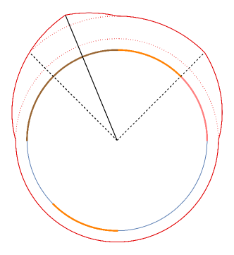
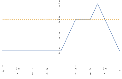
Figure 2. Example 4: A distribution $P\in\mathcal{P}\left({\mathbb{S}^{1}}\right)$ that does not satisfy the condition of strict monotonicity (25) at $\alpha=3/8$. In the left panel, the outer red curve corresponds to the ahD of $x(\theta)=(\cos(\theta),\sin(\theta))^{\mathsf{T}}\in\mathbb{S}^{1}$ as a function of the angle $\theta\in(-\pi,\pi]$; the depth ahD is maximized at the angle $\theta=5\pi/8$ (solid straight line), and $ahD_{3/8}(P)$ corresponds to the angles $\theta\in[\pi/4,3\pi/4]$ (wedge with dashed boundary lines). The depth ahD is constant for $\theta\in[\pi/4,\pi/2]$, meaning that ahD is not strictly monotone for $P$. In the right panel, we have the function $\theta\mapsto ahD(x(\theta);P)$ (blue curve).

The minimum $P$-mass of a hemisphere is $1/8$, and $ahD(x;P)=1/8$ for all $x\in\mathbb{S}^{1}_{-}\cup\mathbb{S}^{1}_{0}$. For $x=(\cos(\theta),\sin(\theta))^{\mathsf{T}}\in\mathbb{S}^{1}$ we get ahD

(28) $$ahD(x;P)=\begin{cases}1/8&\mbox{for }\theta\in(-\pi,0],\\ 1/8+\theta/\pi&\mbox{for }\theta\in(0,\pi/4],\\ 3/8&\mbox{for }\theta\in(\pi/4,\pi/2],\\ 1/2-\frac{\left|\theta-5\pi/8\right|}{\pi}&\mbox{for }\theta\in(\pi/2,3\pi/4],\\ 1/8+\frac{\pi-\theta}{\pi}&\mbox{for }\theta\in(3\pi/4,\pi].\end{cases}$$

In particular, for $\alpha=3/8$ we have that $ahD_{\alpha}(P)$ corresponds to the interval of angles $\theta\in[\pi/4,3\pi/4]$, but the (spherical) closure of the set $\left\{x\in\mathbb{S}^{1}\colon ahD(x;P)>3/8\right\}$ is the interval of angles $\theta\in[\pi/2,3\pi/4]$. The strict monotonicity condition (25) is, therefore, not satisfied for $\alpha=3/8$.

Construct now for $\varepsilon>0$ small and fixed a sequence of measures $\left\{P_{n}\right\}_{n=1}^{\infty}\subset\mathcal{P}\left({\mathbb{S}^{1}}\right)$ defined as similarly as $P$, but in the interval $\theta\in(\pi/2,\pi]$ we put $P_{n}$-mass $1/2+(-1)^{n}\varepsilon$, and in the interval $(0,\pi/4]$ we assign $P_{n}$-mass $1/4+(-1)^{n+1}\varepsilon$. In other words, for $n$ odd we increase the mass in $(0,\pi/4]$ slightly above $1/4$ and decrease the mass in $(\pi/2,\pi]$ below $1/2$, and for $n$ even the other way around. We certainly have that $P_{n}$ converges weakly to $P$ as $n\to\infty$, and since $P$ satisfies the smoothness condition (S), Theorem 10 also gives that $\sup_{x\in\mathbb{S}^{1}}\left|ahD(x;P_{n})-ahD(x;P)\right|$ vanishes as $n\to\infty$. Nevertheless, a simple computation as in (28) gives that for $\alpha=3/8$ we have $ahD_{\alpha}(P_{n})$ contains the interval of angles $\theta\in(\pi/4,\pi/2]$ for $n$ odd, but not for $n$ even. As such, the sequence of sets $\left\{ahD_{\alpha}(P_{n})\right\}_{n=1}^{\infty}$ does not converge in the Hausdorff distance to any set, and (27) cannot be true.

Note that the problem with Example 4 does not rest in the fact that the support of $P$ is disconnected; one could easily add another mixture component supported on $\mathbb{S}^{1}$ to $P$ with sufficiently low weight, and the same phenomenon appears. The core of the problem is in the symmetry of $P$ in the angle $\theta\in[\pi/4,\pi/2)$, giving that any halfspace $H_{u}\in\mathcal{H}_{0}$ with $u=(\cos(\theta),\sin(\theta))^{\mathsf{T}}$ and $\theta\in[3\pi/4,\pi/2]$ has the same $P$-mass equal to $\alpha=3/8$. One natural way of enforcing (25) is to forbid these symmetries, as done in the following result.

Theorem 12.

Suppose that $P\in\mathcal{P}\left({\mathbb{S}^{d-1}}\right)$ has a dominant hemisphere, meaning that there exists $u\in\mathbb{S}^{d-1}$ such that for all $B\subseteq\mathbb{S}^{d-1}\cap H_{u}$ of non-null spherical Lebesgue measure we have $P(B)>P(-B)$. Assume, in addition, that $P$ is smooth in the sense of (S). Then is the condition (25) satisfied for $P$.

Another way of obtaining the strict monotonicity condition (25) is to use directly Theorem 1 and assume that $P$ is supported in a hemisphere $H$. Then, we can assume that after gnomonic projection to the tangent hyperplane at the pole of $H$, the (non-negative) measure $P_{\pm}$ in $\mathbb{R}^{d-1}$ satisfies smoothness and contiguity of its support as assumed in Laketa and Nagy, (2022, Section 4.3).

4.4. Large sample properties

As our final result, we consider the problem of estimating ahD from a random sample. We consider a sequence $X_{1},\dots,X_{n}\in\mathbb{S}^{d-1}$ of independent random variables defined on $\Omega$ sampled from the distribution $P\in\mathcal{P}\left({\mathbb{S}^{d-1}}\right)$. We attach to each $X_{i}\equiv X_{i}(\omega)$ mass $1/n$ and denote the resulting (random) empirical measure by $P_{n}(\omega)\in\mathcal{P}\left({\mathbb{S}^{d-1}}\right)$. When computing the depth, we typically estimate the depth of the (unknown) distribution $P$ by means of the sample depth, based on plugging the empirical measure $P_{n}(\omega)$ into the depth (3) instead of $P$. The depth $ahD(x;P_{n}(\omega))$ is called the sample angular halfspace depth of $x$. In the following result, we prove that the sample ahD almost surely uniformly approximates its population counterpart $ahD(\cdot;P)$ as $n\to\infty$, and the same is true for the derived quantities $\mathfrak{M}(P_{n}(\omega))$ and $ahD_{\alpha}(P_{n}(\omega))$.

Theorem 13.

Suppose that $X_{1},X_{2},\dots,$ is a sequence of independent random variables with distribution $P\in\mathcal{P}\left({\mathbb{S}^{d-1}}\right)$, and let $P_{n}(\omega)\in\mathcal{P}\left({\mathbb{S}^{d-1}}\right)$ be the (random) empirical measure corresponding to $X_{1}(\omega),\dots,X_{n}(\omega)$.

1. Then we have

   $$\mathsf{P}\left(\left\{\omega\in\Omega\colon\lim_{n\to\infty}\sup_{x\in\mathbb{S}^{d-1}}\left|ahD(x;P_{n}(\omega))-ahD(x;P)\right|=0\right\}\right)=1.$$

2. If $P\in\mathcal{P}\left({\mathbb{S}^{d-1}}\right)$ is such that ahD is strictly monotone for $P$, then for any closed interval $A\subset(\min_{x\in\mathbb{S}^{d-1}}ahD(x;P),\max_{x\in\mathbb{S}^{d-1}}ahD(x;P))$ we can write

   $$\mathsf{P}\left(\left\{\omega\in\Omega\colon\lim_{n\to\infty}\sup_{\alpha\in A}\delta_{H}\left(ahD_{\alpha}(P_{n}(\omega)),ahD_{\alpha}(P)\right)=0\right\}\right)=1.$$

3. If $P\in\mathcal{P}\left({\mathbb{S}^{d-1}}\right)$ satisfies the conditions of part (iii) of Theorem 9, then

   $$\mathsf{P}\left(\left\{\omega\in\Omega\colon\lim_{n\to\infty}\delta_{H}\left(\mathfrak{M}(P_{n}(\omega)),\mathfrak{M}(P)\right)=0\right\}\right)=1.$$

Appendix A Proofs of the theoretical results

A.1. Proof of Theorem 1

In the definition of ahD in (3) we only consider halfspaces in $\mathbb{R}^{d}$ whose boundary passes through the origin. Denote by $G_{u}$ the intersection of $\mathcal{G}$ and $H_{0,u}\in\mathcal{H}_{0}$. When considered as a subset of the affine space $\mathcal{G}$, the set $G_{u}$ is a generalized halfspace: (i) it is a halfspace in $\mathcal{G}$ if $u\in\mathbb{S}^{d-1}\setminus\left\{e_{d},-e_{d}\right\}$, (ii) an empty set if $u=-e_{d}$, and (iii) equals $\mathcal{G}$ if $u=e_{d}$. By the definition (9) of the gnomonic projection $\xi$, a point $y\in\mathbb{S}^{d-1}\setminus\mathbb{S}^{d-1}_{0}$ lies in $H_{0,u}$ if and only if $\left\langle y,u\right\rangle=\left\langle\xi(y),u\right\rangle\left\langle y,e_{d}\right\rangle\geq 0$. If $y\in\mathbb{S}^{d-1}_{+}$, this is equivalent with $\xi(y)\in G_{u}=H_{0,u}\cap\mathcal{G}$; for $y\in\mathbb{S}^{d-1}_{-}$ we have that $y\in H_{0,u}$ if and only if $\left\langle\xi(y),u\right\rangle\leq 0$, that is $\xi(y)\in G_{-u}$. In terms of $P_{\pm}$ we can thus express the $P$-mass of any $H_{0,u}\in\mathcal{H}_{0}$ as

(29) $$P\left(H_{0,u}\right)=P_{+}\left(G_{u}\right)+P_{-}\left(G_{-u}\right).$$

Writing $G_{u}^{\circ}$ and $\partial G_{u}$ for the relative interior and the relative boundary of the $(d-1)$-dimensional generalized halfspace $G_{u}$ in $\mathcal{G}$, for any $u\in\mathbb{S}^{d-1}$ we have $P\left(\mathbb{S}^{d-1}_{-}\right)=P_{-}\left(\mathcal{G}\right)=P_{-}\left(G_{-u}^{\circ}\right)+P_{-}\left(\partial G_{-u}\right)+P_{-}\left(G_{u}^{\circ}\right)=P_{-}\left(G_{-u}\right)+P_{-}\left(G_{u}^{\circ}\right)$, simply because the sets $G_{-u}$ and $G_{u}^{\circ}$ are disjoint and decompose $\mathcal{G}$. Thus, we can rewrite (29) to

(30) $$P\left(H_{0,u}\right)=P\left(\mathbb{S}^{d-1}_{-}\right)+P_{+}\left(G_{u}\right)-P_{-}\left(G_{u}^{\circ}\right).$$

This holds true for any normal vector $u\in\mathbb{S}^{d-1}$, including $u=e_{d}$ or $-e_{d}$.

Since we assumed in (8) that $x\in\mathbb{S}^{d-1}_{+}$, we know that $x\in H_{0,u}$ if and only if $\xi(x)\in G_{u}$. Plugging (30) into (3) we obtain

$$ahD(x;P) =P\left(\mathbb{S}^{d-1}_{-}\right)+\inf\left\{P_{+}\left(G_{u}\right)-P_{-}\left(G_{u}^{\circ}\right)\colon u\in\mathbb{S}^{d-1}\mbox{ and }x\in H_{0,u}\right\}$$

$$=P\left(\mathbb{S}^{d-1}_{-}\right)+\inf\left\{P_{+}\left(G_{u}\right)-P_{-}\left(G_{u}^{\circ}\right)\colon u\in\mathbb{S}^{d-1}\mbox{ and }\xi(x)\in G_{u}\right\}$$

$$=P\left(\mathbb{S}^{d-1}_{-}\right)+\inf\left\{P_{+}\left(H\right)-P_{-}\left(H^{\circ}\right)\colon H\in\mathcal{H}^{*}\mbox{ and }\xi(x)\in H\right\}$$

where in the last expression, it makes no difference whether the generalized halfspaces $\mathcal{H}^{*}$ are considered in $\mathbb{R}^{d}$, or $\mathcal{G}$, or $\mathbb{R}^{d-1}$ when identified with $\mathcal{G}$. Considering $\mathcal{H}^{*}$ in $\mathbb{R}^{d-1}$, we have proved the first part of our theorem.

Suppose now that $P_{-}$ satisfies the continuity condition (12). Then, $P_{-}(\partial H)=0$ for all $H\in\mathcal{H}^{*}$ in $\mathbb{R}^{d-1}$ and thus $P_{-}(H^{\circ})=P_{-}\left(H\right)$, which allows us to write $P_{+}\left(H\right)-P_{-}\left(H^{\circ}\right)=P_{+}(H)-P_{-}(H)=P_{\pm}(H)$ in (11).

A.2. Proof of Theorem 3

We first use the portmanteau theorem (Dudley,, 2002, Theorem 11.1.1) to show that the function

(31) $$f\colon\mathcal{P}\left({\mathbb{S}^{d-1}}\right)\times\mathbb{S}^{d-1}\to[0,1]\colon\left(P,u\right)\mapsto P\left(H_{0,u}\right)$$

is upper semi-continuous at any measure $P\in\mathcal{P}\left({\mathbb{S}^{d-1}}\right)$, and continuous at any $P$ that satisfies (S). To see that, fix $P\in\mathcal{P}\left({\mathbb{S}^{d-1}}\right)$ and take $u_{n}\to u$ in $\mathbb{S}^{d-1}$. Since $u_{n}$ converges to $u$, it is possible to find a sequence of orthogonal matrices $\left\{O_{n}\right\}_{n=1}^{\infty}\subset\mathbb{R}^{d\times d}$ such that $O_{n}u_{n}=u$ for each $n=1,2,\dots$, and $O_{n}$ converges to the identity matrix $I_{d}\in\mathbb{R}^{d\times d}$. Define a measure $Q_{n}\in\mathcal{P}\left({\mathbb{S}^{d-1}}\right)$ as the distribution of $O_{n}X_{n}$ with $X_{n}\sim P_{n}$. By Slutsky’s theorem (Jiang,, 2010, Theorem 2.13), we then have that $Q_{n}\xrightarrow{w}P$ as $n\to\infty$. At the same time, for each $n=1,2,\dots$ we can write

$$O_{n}H_{0,u_{n}}=\left\{O_{n}y\colon\left\langle y,u_{n}\right\rangle\geq 0\right\}=\left\{z\colon\left\langle O_{n}^{\mathsf{T}}z,u_{n}\right\rangle\geq 0\right\}=H_{0,O_{n}u_{n}},$$

where we used $O_{n}^{-1}=O_{n}^{\mathsf{T}}$ as follows from the orthogonality of $O_{n}$ and therefore, we have

(32) $$P_{n}(H_{0,u_{n}})=\mathsf{P}\left(X_{n}\in H_{0,u_{n}}\right)=\mathsf{P}\left(O_{n}X_{n}\in O_{n}H_{0,u_{n}}\right)=Q_{n}(H_{0,u}).$$

Thus, we have a fixed closed halfspace $H_{0,u}$ and a sequence of measures $\left\{Q_{n}\right\}_{n=1}^{\infty}\subset\mathcal{P}\left({\mathbb{S}^{d-1}}\right)$ such that $Q_{n}\xrightarrow{w}P$ as $n\to\infty$. The portmanteau theorem (Dudley,, 2002, Theorem 11.1.1) and (32) then give that

$${\lim\sup}_{n\to\infty}f(P_{n},u_{n})={\lim\sup}_{n\to\infty}P_{n}(H_{0,u_{n}})={\lim\sup}_{n\to\infty}Q_{n}(H_{0,u})\leq P(H_{0,u})=f(P,u)$$

as we wanted to show. In the special case when also (S) is valid, we obtain that $H_{0,u}$ is a continuity set of $P$, and the portmanteau theorem gives even

$${\lim}_{n\to\infty}f(P_{n},u_{n})={\lim}_{n\to\infty}P_{n}(H_{0,u_{n}})={\lim}_{n\to\infty}Q_{n}(H_{0,u})=P(H_{0,u})=f(P,u).$$

Now for $x\in\mathbb{S}^{d-1}$ denote

(33) $$v(x)=\left\{u\in\mathbb{S}^{d-1}\colon x\in H_{0,u}\right\}=\left\{u\in\mathbb{S}^{d-1}\colon\left\langle x,u\right\rangle\geq 0\right\}=\mathbb{S}^{d-1}\cap H_{0,x}$$

the set of all inner normals of halfspaces taken in the infimum in the definition (3) of $ahD(x;P)$. The set-valued mapping $v(x)$ is continuous in $x$ in the sense of Painlevé-Kuratowski convergence (Rockafellar and Wets,, 1998, Chapter 5.B), and ahD can be written as

$$ahD\left(x;P\right)=\inf_{u\in v(x)}f(P,u).$$

We have verified all the assumptions of Berge’s maximum theorem (Berge,, 1997, pp. 115–117) on parametric optimization, which asserts that the depth function $ahD\colon\mathbb{S}^{d-1}\times\mathcal{P}\left({\mathbb{S}^{d-1}}\right)\to[0,1]\colon(x,P)\mapsto ahD(x;P)$ is upper semi-continuous in both arguments for general $P$, and continuous in both arguments at any $P$ satisfying (S).

A.3. Proof of Theorem 4

Suppose first that $x\in ahD_{\alpha}(P)$, meaning that $ahD\left(x;P\right)\geq\alpha$. If $x$ does not belong to the right-hand side of (18), then there must exist an open halfspace $G$ whose boundary passes through the origin, $P(G^{\mathsf{c}})<\alpha$, and $x\notin G$. Take $H=G^{\mathsf{c}}\in\mathcal{H}_{0}$. Now, we have $x\in H\in\mathcal{H}_{0}$ and $P(H)<\alpha$, which contradicts $ahD\left(x;P\right)\geq\alpha$. Necessarily, $ahD_{\alpha}(P)\subseteq\bigcap\left\{G\colon G^{\mathsf{c}}\in\mathcal{H}_{0}\mbox{ and }P(G^{\mathsf{c}})<\alpha\right\}$.

For the other direction, suppose that $x\notin ahD_{\alpha}(P)$. Then we have $\alpha>ahD(x;P)=\inf_{H\in\mathcal{H}_{0}\colon x\in H}P(H)$, meaning that there exists a closed halfspace $H\in\mathcal{H}_{0}$ such that $x\in H$ and $P(H)<\alpha$. Consider the open halfspace $G=H^{\mathsf{c}}$. Then $x\notin G$, $G^{\mathsf{c}}\in\mathcal{H}_{0}$ and $P(G^{\mathsf{c}})=P(H)<\alpha$, meaning that $x$ does not belong to the right-hand side of (18). This gives $ahD_{\alpha}(P)\supseteq\bigcap\left\{G\colon G^{\mathsf{c}}\in\mathcal{H}_{0}\mbox{ and }P(G^{\mathsf{c}})<\alpha\right\}$, and proves our claim.

A.4. Proof of Theorem 5

Take any $x\in\mathbb{S}^{d-1}$ that is not in $ahD_{\alpha}(P)$. Then $ahD\left(x;P\right)<\alpha$ and therefore, there is a closed halfspace $H\in\mathcal{H}_{0}$ such that $x\in H$ and $P(H)<\alpha$. First, we show that we can also assume that $H$ satisfies the additional property $x\in H^{\circ}$. Indeed, if $x\in\partial H$ and $u\in\mathbb{S}^{d-1}$ is the inner normal of $H$, we choose $u_{n}=\cos(1/n)u+\sin(1/n)x$ for $n=1,2,\dots$. Since $\left\langle x,u\right\rangle=0$ we have

$$\left\|u_{n}\right\|^{2}=(\cos(1/n))^{2}\left\langle u,u\right\rangle+(\sin(1/n))^{2}\left\langle x,x\right\rangle=1,$$

and thus $u_{n}\in\mathbb{S}^{d-1}$. In addition,

$$\left\langle x,u_{n}\right\rangle=\cos(1/n)\left\langle x,u\right\rangle+\sin(1/n)\left\langle x,x\right\rangle=\sin(1/n)>0,$$

and for $H_{n}=H_{0,u_{n}}$ we can write $x\in H_{n}^{\circ}$ for all $n$. Halfspaces $H_{n}\in\mathcal{H}_{0}$ correspond to slightly tilted $H$ so that $x$ is moved to the interior of $H_{n}$. In the proof of Theorem 3, we proved that the function (31) given by $u\mapsto P(H_{0,u})$ is upper semi-continuous. Since $u_{n}\to u$, we thus have

$$\limsup_{n\rightarrow\infty}P(H_{n})\leq P(H)<\alpha.$$

Necessarily, there must exist $n=1,2,\dots$ such that $P(H_{n})<\alpha$. For such $n$ we have $x\in H_{n}^{\circ}$ as we wanted to show.

Take now this $H\in\mathcal{H}_{0}$ with the properties $x\in H^{\circ}$ and $P(H)<\alpha$, and denote by $\tilde{H}=(H^{\circ})^{\mathsf{c}}$ the complementary closed halfspace. Then $x\notin\tilde{H}$, but $\tilde{H}\in\mathcal{H}_{0}$ and $P(\tilde{H}^{\mathsf{c}})=P(H^{\circ})\leq P(H)<\alpha$. Thus, $x$ does not belong to the left-hand side of (19).

A.5. Example to Theorems 4 and 5

It is convenient to define $P\in\mathcal{P}\left({\mathbb{S}^{2}}\right)$ by means of its gnomonic projection $P_{\pm}\in\mathcal{S}\left({\mathbb{R}^{2}}\right)$ from (10). We then project $P_{\pm}$ to $\mathbb{S}^{2}$ to obtain $P$, and use formula (11) to evaluate ahD. For that we simplify the notation and write for $y\in\mathbb{R}^{2}$

$$shD\left(y;P_{\pm}\right)=\inf\left\{P_{\pm}\left(H\right)+P_{-}\left(\partial H\right)\colon H\in\mathcal{H}^{*}\mbox{ and }y\in H\right\},$$

giving by (11) that $ahD(x;P)=P\left(\mathbb{S}^{d-1}_{-}\right)+shD\left(\xi(x);P_{\pm}\right)$.

We take the signed measure $P_{\pm}\in\mathcal{S}\left({\mathbb{R}^{2}}\right)$ with three atoms, of $P_{\pm}$-mass $1/5$ each, at points $y_{1}=(-1,0)^{\mathsf{T}}$, $y_{2}=(0,0)^{\mathsf{T}}$ and $y_{3}=(1,0)^{\mathsf{T}}$, and two atoms, of mass $-1/5$ each, at points $z_{1}=(0,-1)^{\mathsf{T}}$ and $z_{2}=(0,1)^{\mathsf{T}}$. The total $P_{\pm}$-mass of $\mathbb{R}^{2}$ is $1/5$; any closed halfspace $H\subset\mathbb{R}^{2}$ that contains both $z_{1}$ and $z_{2}$ must also contain $y_{2}$. Thus, no closed halfspace in $\mathbb{R}^{2}$ can have $P_{\pm}$-mass smaller than $-1/5$, and $shD(y;P_{\pm})\geq-1/5$ for all $y\in\mathbb{R}^{2}$. A halfspace $H$ with $P_{\pm}(H)=-1/5$ and $y\in H$ that does not contain any atoms of $P_{\pm}$ in $\partial H$ can be found for any $y\notin A$, where $A$ is the closed line segment between $y_{1}$ and $y_{3}$. Thus, $shD(y;P_{\pm})=-1/5$ for all $y\notin A$. For any $y\in A$, we can always find a halfspace $H$ with $P_{\pm}(H)=0$ and $y\in H$. We have that $shD(y;P_{\pm})=0$ for $y\in A$.

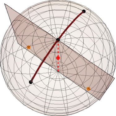
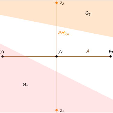
Figure 3. The setup from Appendix A.5: The five points on the sphere $\mathbb{S}^{2}$ (three black points in $\mathbb{S}^{2}_{+}$ and two orange points in $\mathbb{S}^{2}_{-}$; the origin is displayed in red. The depth ahD of the corresponding measure is equal to $1/5$ for all $x\notin B$ and $2/5$ for all $x\in B$, where $B$ is the arc displayed in brown. The plane on the left-hand side passing through the origin separates $\mathbb{R}^{3}$ into two open halfspaces, each containing only a single black point. In the right-hand panel, we see the same setup in the gnomonic projection in the plane $\mathbb{R}^{2}$. The pink halfplane $G_{1}$ contains $P_{\pm}$-mass $0$, while the orange one $G_{2}$ contains $P_{\pm}$-mass $-1/5$.

We now use the inverse gnomonic projection and formula (11) to transfer our setup from $\mathbb{R}^{2}$ to $\mathbb{S}^{2}$. The points $y_{1}$, $y_{2}$, $y_{3}$ map to $x_{1}=(-1/\sqrt{2},0,1/\sqrt{2})^{\mathsf{T}}$, $x_{2}=(0,0,1)^{\mathsf{T}}$, $x_{3}=(1/\sqrt{2},0,1/\sqrt{2})^{\mathsf{T}}$ in $\mathbb{S}^{2}_{+}$, while $z_{1}$ and $z_{2}$ map to $x_{4}=(0,-1/\sqrt{2},-1/\sqrt{2})^{\mathsf{T}}$ and $(0,1/\sqrt{2},-1/\sqrt{2})^{\mathsf{T}}$, respectively. Our atomic measure $P\in\mathcal{P}\left({\mathbb{S}^{2}}\right)$ has five atoms $x_{i}$, $i=1,\dots,5$, each of $P$-mass $1/5$. Using Theorem 1 we get that $ahD(x;P)=1/5$ for all $x\in\mathbb{S}^{2}\setminus B$ and $ahD(x;P)=2/5$ for $x\in B$, where $B=\left\{\cos(\alpha)x_{1}+\sin(\alpha)x_{3}\colon\alpha\in[0,\pi/2]\right\}$ is the shorter arc between $x_{1}$ and $x_{3}$. We obtain $ahD_{2/5}(P)=B$. Take now a closed halfspace $H=H_{0,u}\in\mathcal{H}_{0}$ with $u=(1,0,0)^{\mathsf{T}}$. We have $P(H^{\mathsf{c}})=P(\{x_{1}\})=1/5<2/5$, but $H\cap ahD_{2/5}(P)$ is one half of the arc $B$. Thus, for $\alpha=2/5$ and, say, $x_{1}\in ahD_{\alpha}(P)$ we have $H\in\mathcal{H}_{0}$ that satisfies $P(H^{\mathsf{c}})<\alpha$, but $x_{1}\notin H$. Therefore, the inequality in (19) is strict.

A.6. Proof of Theorem 6

The proof is a direct adaptation of the proof of Pokorný et al., (2023, Theorem 1).

A.7. Proof of Theorem 7

The first part of the statement follows directly from Pokorný et al., (2023, Theorem 1). Indeed, the right-hand side of (21) is by that theorem precisely the (Euclidean) halfspace depth of the origin $0\in\mathbb{R}^{d}$ w.r.t. the measure $P$ when considered in the ambient space $\mathbb{R}^{d}$. Theorem 1 in Pokorný et al., (2023) then states that $hD(0;P)$ can also be expressed in terms of our flag halfspaces (20), and a flag halfspace satisfying (21) always exists.

For the second part of our claim, note that since by Theorem 6 also ahD can be expressed using flag halfspaces, for every $x\in F$ from (21), we must have $ahD(x;P)=P(F)$, directly because of (21) and the definition (3) of ahD.

A.8. Proof of Theorem 8

For any orthogonal matrix $O\in\mathbb{R}^{d\times d}$ such that $O\mu=\mu$ we know, by the assumption of rotational symmetry of $P$, that $P_{OX}=P$. Thanks to the rotational invariance ($\mathrm{D}_{1}$) of ahD from Theorem 2 we get

(34) $$ahD(x;P)=ahD(Ox;P_{OX})=ahD(Ox;P).$$

Thus, ahD of $x\in\mathbb{S}^{d-1}$ must be constant on spheres that are cut from $\mathbb{S}^{d-1}$ by hyperplanes orthogonal to $\mu$. In other words, $ahD(x;P)$ depends only on $\left\langle x,\mu\right\rangle$.

By Theorem 7, we know that (at least) one of the points $\mu,-\mu\in\mathbb{S}^{d-1}$ lies in the region of minimum ahD of $P$. Without loss of generality, let $-\mu$ be this point, meaning that

(35) $$ahD(-\mu;P)=\min_{x\in\mathbb{S}^{d-1}}ahD(x;P).$$

We will show that $ahD(\mu;P)=\max_{x\in\mathbb{S}^{d-1}}ahD(x;P)$. Suppose for contradiction that there exists $y\in\mathbb{S}^{d-1}\setminus\left\{\mu,-\mu\right\}$ such that

(36) $$\alpha=ahD(y;P)>ahD(\mu;P)\geq ahD(-\mu;P),$$

the second inequality following trivially from (35). In that case, formula (34) gives that $ahD(x;P)=\alpha$ for all points $x$ on the set $S=\left\{x\in\mathbb{S}^{d-1}\colon\left\langle x,\mu\right\rangle=\left\langle y,\mu\right\rangle\right\}$. Necessarily, $ahD_{\alpha}(P)\supseteq S$ but $\mu,-\mu\notin ahD_{\alpha}(P)$. By Theorem 4, the set $ahD_{\alpha}(P)$ must be spherically convex, meaning that the convex hull of $\mathrm{rad}\left(S\right)$ intersected with $\mathbb{S}^{d-1}$ is a subset of $ahD_{\alpha}(P)$. Now, if $\left\langle y,\mu\right\rangle\neq 0$, the convex hull of $\mathrm{rad}\left(S\right)$ necessarily contains either $\mu$ or $-\mu$, which would contradict (36). The only remaining case is that $\left\langle y,\mu\right\rangle=0$. That is, however, also impossible thanks to our Theorem 7 that entails (22). Indeed, if for some $y\in S$ we had (36), then (22) gives that $ahD(-y;P)=ahD(-\mu;P)<\alpha$, but at the same time $-y\in S$ gives $ahD(-y;P)=\alpha$, a contradiction. We have found that one of the points $\mu$ or $-\mu$ must maximize the angular halfspace depth of $P$ as we wanted to show.

A.9. Proof of Theorem 9

The following auxiliary lemma will be useful.

Lemma 14.

Let $U\subset\mathbb{S}^{d-1}$ be a set that is either open or finite in the sphere $\mathbb{S}^{d-1}$. The following are equivalent:

1. the origin lies in the convex hull of $U$;

2. the origin lies in the convex hull of $R=\mathrm{rad}\left(U\right)$;

3. $\bigcup_{r\in R}H_{0,r}=\mathbb{S}^{d-1}$;

4. $\bigcup_{u\in U}H_{0,u}=\mathbb{S}^{d-1}$.

Proof of Lemma 14.

Since $U\subset R$, the convex hull of $U$ is a subset of the convex hull of $R$, and (A) implies (B). For the opposite implication, suppose that the origin lies in the convex hull of $R$. Carathéodory’s theorem (Schneider,, 2014, Theorem 1.1.4) gives that there exists $d+1$ (not necessarily distinct) points $r_{1},\dots,r_{d+1}\in R$ such that

(37) $$0=\sum_{i=1}^{d+1}\lambda_{i}\,r_{i}\mbox{ for some $0\leq\lambda_{i}$ with $\sum_{i=1}^{d+1}\lambda_{i}=1$.}$$

Since $R=\mathrm{rad}\left(U\right)$, being a radial extension, never contains the origin $0\in\mathbb{R}^{d}$, we have that $\sum_{i=1}^{d+1}\lambda_{i}\left\|r_{i}\right\|>0$. From (37) we see that

$$\sum_{i=1}^{d+1}\frac{\lambda_{i}\left\|r_{i}\right\|}{\sum_{j=1}^{d+1}\lambda_{j}\left\|r_{j}\right\|}\frac{r_{i}}{\left\|r_{i}\right\|}=0,$$

and setting $u_{i}=r_{i}/\left\|r_{i}\right\|\in U$ and $\gamma_{i}=\lambda_{i}\left\|r_{i}\right\|/\left(\sum_{j=1}^{d+1}\lambda_{j}\left\|r_{j}\right\|\right)$ yields that the origin is also contained in the convex hull of $U$. Therefore (B) implies (A).

Statements (C) and (D) are clearly equivalent since $H_{0,r}=H_{0,u}$ for each $r\in R$ and $u=r/\left\|r\right\|$.

Note that if $U$ is supposed to be open in the sphere, then the set $R$ from (B) is open in $\mathbb{R}^{d}$. By Schneider, (2014, Theorem 1.1.10), we then know that the convex hull $C$ of $R$ is open in $\mathbb{R}^{d}$. Suppose first that (B) is not true. The Hahn-Banach theorem (Schneider,, 2014, Theorem 1.3.4) gives that there exists a vector $x\in\mathbb{S}^{d-1}$ such that $H_{0,x}\cap C=\emptyset$, or equivalently $\left\langle x,r\right\rangle<0$ for all $r\in C$. The strict inequality follows either from the fact that $C$ is open (in the case of $U$ open), or from the finiteness of $U$. The inequality $\left\langle x,r\right\rangle<0$ however translates into $x\notin H_{0,r}$ for all $r\in R$, which gives that also (C) cannot be true.

Suppose finally that (C) is violated. Then there exists $x\in\mathbb{S}^{d-1}$ that is not contained in any $H_{0,r}$, or equivalently $\left\langle x,r\right\rangle<0$ for all $r\in R$. If the origin was contained in the convex hull $C$ of $R$, Schneider, (2014, Theorem 1.1.4) again gives that we could write (37) for some $r_{1},\dots,r_{d+1}\in R$. The inner product of (37) with $x$ then gives $0=\sum_{i=1}^{d+1}\lambda_{i}\,\left\langle x,r_{i}\right\rangle<0$, a contradiction. Thus, (B) implies (C), and the lemma is proved. ∎

Part (i). We begin by showing that the depth $\alpha^{*}(P)$ of an ahD-median cannot be less than $1/(d+1)$. Suppose for contradiction that for some $P\in\mathcal{P}\left({\mathbb{S}^{d-1}}\right)$ we have $\alpha^{*}(P)<c<1/(d+1)$ for $c>0$. Then, for any $x\in\mathbb{S}^{d-1}$ there exists a halfspace $H_{0,u(x)}\in\mathcal{H}_{0}$ that contains $x$, and $P(H_{0,u(x)})<c$. In other words, there is a covering of $\mathbb{S}^{d-1}$ by halfspaces whose $P$-probability is less than $c$. Consider the collection of all inner normals $U=\left\{u(x)\right\}_{x\in\mathbb{S}^{d-1}}$ of such halfspaces. By the upper semi-continuity of function $f$ from (31), the lower level set $U$ of $f$ is open in $\mathbb{S}^{d-1}$ (Rockafellar and Wets,, 1998, Theorem 1.6). The auxiliary Lemma 14 below then gives that the origin must be contained in the convex hull of $U$. Carathéodory’s theorem (Schneider,, 2014, Theorem 1.1.4), in turn, gives that in that case, the origin must be contained in a convex hull of at most $d+1$ (not necessarily distinct) elements of the set $U$ denoted by $u_{1},\dots,u_{d+1}\in\mathbb{S}^{d-1}$. Using once again Lemma 14, we have that these $d+1$ elements induce a covering of $\mathbb{R}^{d}$, that is $\bigcup_{i=1}^{d+1}H_{0,u_{i}}=\mathbb{R}^{d}$ with $P\left(H_{0,u_{i}}\right)<c$ for all $i=1,\dots,d+1$. That means

$$1=P\left(\mathbb{R}^{d}\right)=P\left(\bigcup_{i=1}^{d+1}H_{0,u_{i}}\right)\leq\sum_{i=1}^{d+1}P\left(H_{0,u_{i}}\right)\leq(d+1)c<1,$$

a contradiction.

For the upper semi-continuity of the maximum depth mapping $\alpha^{*}$, Theorem 3 gives that the function $ahD\left(\cdot;\cdot\right)$ is upper semi-continuous in both arguments. Berge’s maximum theorem (Berge,, 1997, Theorem 2 on p. 116) then directly yields the conclusion.

Part (ii). Under the smoothness assumption (S), Theorem 3 gives that $ahD\left(\cdot;\cdot\right)$ is continuous at $P$. Berge, (1997, Maximum theorem on p. 117) then entails the continuity of $\alpha^{*}$, and the outer semi-continuity of $\mathfrak{M}$.

Now, let $x\in\mathfrak{M}(P)$. Take any hyperplane $G$ containing $x$ and the origin in $\mathbb{R}^{d}$, and consider the two halfspaces $H,H^{\prime}\in\mathcal{H}_{0}$ determined by $G$. Because $P$ is smooth, we have $P(G)=0$ and consequently $P(H)+P(H^{\prime})=1$, which gives $\alpha^{*}(P)=ahD(x;P)\leq\min\left\{P(H),1-P(H)\right\}\leq 1/2$.

Part (iii). By Theorem 3 we know that $x_{n}\in\mathfrak{M}(P_{n})$ always exists. Since $\mathbb{S}^{d-1}$ is a compact set, there exists a sub-sequence $\left\{x_{n(k)}\right\}_{k=1}^{\infty}$ of that sequence of directional medians such that $x_{n(k)}$ converges in $\mathbb{S}^{d-1}$ as $k\to\infty$. Thanks to part (ii) of this theorem, we know that $x_{n(k)}$ then must converge to $x$, the unique median of $P$. We just proved the inner semi-continuity of the median mapping (24), which together with its outer semi-continuity from part (ii) of this theorem gives the continuity of (24) in the sense of Rockafellar and Wets, (1998, Definition 5.4). For a sequence of closed sets $\left\{K_{n}\right\}_{n=1}^{\infty}$ that are all contained in a bounded subset of $\mathbb{R}^{d}$, the convergence in the Hausdorff distance $\lim_{n\to\infty}\delta_{H}\left(K_{n},K\right)=0$ is equivalent with the convergence of sets induced by the notion of continuity of set-valued mappings discussed above (Rockafellar and Wets,, 1998, Chapter 4C and p. 144).

A.10. Proof of Example 2

First note that since $0=\sum_{i=1}^{d+1}e_{i}/(d+1)$, Lemma 14 gives that the collection of halfspaces $H_{0,e_{i}}$, $i=1,\dots,d+1$, covers $\mathbb{S}^{d-1}$. In particular, for any $x\in\mathbb{S}^{d-1}$ there must exist $i=1,\dots,d+1$ such that $\left\langle x,e_{i}\right\rangle\geq 0$, implying $e_{i}\in v(x)$ for $v(x)=\left\{u\in\mathbb{S}^{d-1}\colon x\in H_{0,u}\right\}=\mathbb{S}^{d-1}\cap H_{0,x}$, see also (33). Thus, any halfspace $H_{0,u}\in\mathcal{H}_{0}$ with $u\in v(x)$ contains at least one atom of $P$, and $ahD\left(x;P\right)\geq 1/(d+1)$. We now construct a halfspace in $\mathcal{H}_{0}$ that contains $x$ and exactly one atom of $P$. Since $x=\left(x_{1},\dots,x_{d}\right)^{\mathsf{T}}\in\mathbb{S}^{d-1}$, two situations are possible: (i) either all coordinates of $x$ are non-positive, or (ii) for some $j=1,\dots,d$ the coordinate $x_{j}$ is strictly positive.

In the first case, we consider the halfspace $H_{0,e_{d+1}}$. Then, $\left\langle x,e_{d+1}\right\rangle>0$, i.e. $x\in H_{0,e_{d+1}}$, and at the same time $\left\langle e_{i},e_{d+1}\right\rangle=-1$ for any $i\neq d+1$, meaning that $e_{i}\notin H_{0,e_{d+1}}$. We get that $H_{0,e_{d+1}}$ contains $x$ and $e_{d+1}$, but no other atom of $P$.

In the second case, let $j=1,\dots,d$ be the first index with $x_{j}>0$. Take $\varepsilon>0$ small enough, and consider $u=e_{j}-\left(\varepsilon,\dots,\varepsilon\right)^{\mathsf{T}}$ and the halfspace $H_{0,u/\left\|u\right\|}$. A simple calculation gives

$$\left\langle e_{j},u\right\rangle =1-\varepsilon, \left\langle e_{i},u\right\rangle =-\varepsilon,\mbox{ for $i=1,\dots,d$, $i\neq j$},$$

$$\left\langle x,u\right\rangle =x_{j}(1-\varepsilon)-\varepsilon\sum_{i\neq j}x_{i}, \mbox{ and }\quad\sqrt{d}\left\langle e_{d+1},u\right\rangle =\varepsilon(d-1)-(1-\varepsilon),$$

meaning that for $\varepsilon>0$ small enough, $x,e_{j}\in H_{0,u/\left\|u\right\|}$, but $e_{i}\notin H_{0,u/\left\|u\right\|}$ for all $i=1,\dots,d+1$, $i\neq j$. Thus, $H_{0,u/\left\|u\right\|}$ contains only $x$ and a single atom of $P$, meaning that $ahD\left(x;P\right)=1/(d+1)$.

A.11. Proof of Theorem 10

We have

(38) $$\sup_{x\in\mathbb{S}^{d-1}} \left|ahD(x;P_{n})-ahD(x;P)\right|=\sup_{x\in\mathbb{S}^{d-1}}\left|\inf_{H\in\mathcal{H}_{0}\colon x\in H}P_{n}(H)-\inf_{H\in\mathcal{H}_{0}\colon x\in H}P(H)\right|$$

$$\leq\sup_{x\in\mathbb{S}^{d-1}}\sup_{H\in\mathcal{H}_{0}\colon x\in H}\left|P_{n}(H)-P(H)\right|\leq\sup_{H\in\mathcal{H}_{0}}\left|P_{n}(H)-P(H)\right|.$$

The final expression vanishes as $n\to\infty$ by, e.g., Nagy et al., (2016, Theorem A.3).

A.12. Proof of Theorem 11

We apply the proof of implication (ComD) $\Rightarrow$ (ComR) from Dyckerhoff, (2017, Theorem 4.5). In that paper, only depths in $\mathbb{R}^{d}$ are considered. Nevertheless, the fact that one works in $\mathbb{R}^{d}$ is used only in several arguments in the proofs, and many of the derivations work precisely in the same way for measures in $\mathbb{S}^{d-1}$.

For starters, in Dyckerhoff, (2017, page 4) it is assumed that the function $D$ in $\mathbb{R}^{d}$ must be a depth in the sense of Definition 2.1 in Dyckerhoff, (2017). That requires that the upper level sets $D_{\alpha}(P)=\left\{x\in\mathbb{R}^{d}\colon D(x;P)\geq\alpha\right\}$ are all (R1) affine equivariant (for $\alpha\geq 0$), (R2) bounded (for $\alpha>0$), (R3) closed (for $\alpha>0$), and (R4) star-shaped (for all $\alpha\geq 0$). The requirement (R1) of affine equivariance is, however, not used anywhere in the proof of Theorem 4.5 in Dyckerhoff, (2017). The (spherical counterparts of the) additional conditions R2–R4 are all satisfied for ahD, because • $ahD_{\alpha}(P)\subseteq\mathbb{S}^{d-1}$for all $\alpha\geq 0$ and $\mathbb{S}^{d-1}$ is itself bounded, giving R2, • each $ahD_{\alpha}(P)$ is closed by Theorem 3, which verifies R3, and • (spherical) star-shapedness of $ahD_{\alpha}(P)$ in R4 follows immediately from the (spherical) convexity of $ahD_{\alpha}(P)$ as proved in Theorem 4. Thus, the advances proved in Dyckerhoff, (2017) can be used in our setup.

Mimicking the proof of Theorem 4.5 in Dyckerhoff, (2017) for a depth $D$ in $\mathbb{R}^{d}$, we see that the core of the proof actually lies in proving • the continuity of the function $\alpha\mapsto D_{\alpha}(P)$ in the Hausdorff metric (23), and • the bound

(39) $$D_{\beta+\gamma}(P)\subseteq D_{\beta}(P_{n})\subseteq D_{\beta-\gamma}(P)\quad\mbox{for all $n\geq N$ and $\beta\geq\alpha_{1}$},$$

where $\alpha_{1}$ is the lower endpoint of the interval $A\subset(0,\max_{x\in\mathbb{R}^{d}}D(x;P))$, $\gamma>0$ is a small enough constant, and $N$ is a large enough integer.

The continuity of the mapping $\alpha\mapsto D_{\alpha}(P)$ is obtained in Dyckerhoff, (2017, Theorem 3.2). There, it is asserted that strict monotonicity of the depth $D$ for $P\in\mathcal{P}\left({\mathbb{R}^{d}}\right)$ at all $\alpha\in(0,\max_{x\in\mathbb{R}^{d}}D(x;P))$ is enough to have continuity of $\alpha\mapsto D_{\alpha}(P)$ in $\alpha\in(0,\max_{x\in\mathbb{R}^{d}}D(x;P)]$. The proof of Theorem 3.2 in Dyckerhoff, (2017) does not use the fact that we work in $\mathbb{R}^{d}$; it works equally well in $\mathbb{S}^{d-1}$. In our setup, however, we assume strict monotonicity in (25) only for $\alpha\in(\min_{x\in\mathbb{S}^{d-1}}ahD(x;P),\max_{x\in\mathbb{S}^{d-1}}ahD(x;P))$, which by the same argument gives continuity of $\alpha\mapsto ahD_{\alpha}(P)$ in the Hausdorff distance (23) for $\alpha\in(\min_{x\in\mathbb{S}^{d-1}}ahD(x;P),\max_{x\in\mathbb{S}^{d-1}}ahD(x;P)]$.

As the second ingredient, we need to prove (39) for $D=ahD$. That is implication $(ii)\Rightarrow(iii)$ in Dyckerhoff, (2017, Theorem 4.4). As before, the proof of this implication does not use the fact that the depth $D$ is defined in $\mathbb{R}^{d}$ and also works for $ahD$ in $\mathbb{S}^{d-1}$. In fact, the proof can be simplified by dropping the argument of a bounded set $M$ since, in our setup, we could take $M=\mathbb{S}^{d-1}$ directly. In view of our restriction to $\alpha>\min_{x\in\mathbb{S}^{d-1}}ahD(x;P)$ in proving continuity of $ahD_{\alpha}(P)$, we obtain (39) for all $\beta\geq\alpha_{1}>\min_{x\in\mathbb{S}^{d-1}}ahD(x;P)$.

Putting the two ingredients together, in the proof of implication (ComD) $\Rightarrow$ (ComR) from Dyckerhoff, (2017, Theorem 4.5) we obtain (27) as needed.

Observe that in Dyckerhoff, (2017), two additional conditions are assumed for the depth $D$ throughout the paper:

• The range condition (RC) from page 9 of Dyckerhoff, (2017).

• The “general assumption” stating that for each $\alpha<\max_{x\in\mathbb{S}^{d-1}}ahD(x;P)$ must the set $ahD_{\alpha}(P)$ have non-empty interior.

None of these is necessary for the proof of (27).

A.13. Proof of Theorem 12

The condition of existence of a dominant hemisphere immediately implies that $\mathbb{S}^{d-1}\setminus H_{u}$ is an open hemisphere of minimum depth as in Theorem 6. The smoothness of $P$ and the continuity of ahD in $x$ from Theorem 3 then assert that the whole closed hemisphere $\mathbb{S}^{d-1}\cap H_{-u}$ is of minimum ahD. To prove the strict monotonicity of ahD, we pick any point $x\in\mathbb{S}^{d-1}$ from the ahD-median set of $P$. Because of the smoothness of $P$, we can argue as in Laketa and Nagy, (2022, Lemma 10) to show that $ahD_{\alpha}(P)$ must have non-empty (spherical) interior for all $\alpha\leq\max_{y\in\mathbb{S}^{d-1}}ahD(y;P)$. Further, the dominant hemisphere condition says that for any $H,H^{\prime}\in\mathcal{H}_{0}$ such that $H\cap H_{u}\subset H^{\prime}\cap H_{u}$ we have

$$P(H^{\prime})=P(H^{\prime}\cap H)+P(H^{\prime}\setminus H)>P(H^{\prime}\cap H)+P(H\setminus H^{\prime})=P(H),$$

since $H^{\prime}\cap H\subset H_{u}$. This allows us to use the arguments as in the linear case and hD in parts (iii) and (v) of the proof of Laketa and Nagy, (2022, Theorem 9), which together give (25).

A.14. Proof of Theorem 13

Our first claim can be proved analogously as for Theorem 10. The only exception is that in the final step, the last expression in (38) vanishes as $n\to\infty$ almost surely, because the set of closed halfspaces $\mathcal{H}$ and its subset $\mathcal{H}_{0}$ are both Glivenko-Cantelli classes of sets (van der Vaart and Wellner,, 1996, Section 2.4 and Problem 14 in Section 2.6).

For the second claim, part (i) gives that (26) is valid for $\mathsf{P}$-almost all $\omega\in\Omega$. Thus, we can separately apply Theorem 11 for each $\omega\in\Omega$ and obtain the result.

The last part of our theorem follows by direct application of part (iii) of Theorem 9 and the theorem of Varadarajan (see, e.g., Dudley,, 2002, Theorem 11.4.1).

Acknowledgment

The work of Stanislav Nagy was supported by Czech Science Foundation (EXPRO project n. 19-28231X).

References

- Agostinelli and Romanazzi, (2013) Agostinelli, C. and Romanazzi, M. (2013). Nonparametric analysis of directional data based on data depth. Environ. Ecol. Stat., 20(2):253–270.
- Berge, (1997) Berge, C. (1997). Topological spaces. Dover Publications, Inc., Mineola, NY. Translated from the French original by E. M. Patterson, Reprint of the 1963 translation.
- Besau and Werner, (2016) Besau, F. and Werner, E. M. (2016). The spherical convex floating body. Adv. Math., 301:867–901.
- Buttarazzi et al., (2018) Buttarazzi, D., Pandolfo, G., and Porzio, G. C. (2018). A boxplot for circular data. Biometrics, 74(4):1492–1501.
- Chernozhukov et al., (2017) Chernozhukov, V., Galichon, A., Hallin, M., and Henry, M. (2017). Monge-Kantorovich depth, quantiles, ranks and signs. Ann. Statist., 45(1):223–256.
- Donoho and Gasko, (1992) Donoho, D. L. and Gasko, M. (1992). Breakdown properties of location estimates based on halfspace depth and projected outlyingness. Ann. Statist., 20(4):1803–1827.
- Dudley, (2002) Dudley, R. M. (2002). Real analysis and probability, volume 74 of Cambridge Studies in Advanced Mathematics. Cambridge University Press, Cambridge. Revised reprint of the 1989 original.
- Dyckerhoff, (2017) Dyckerhoff, R. (2017). Convergence of depths and depth-trimmed regions. arXiv preprint arXiv:1611.08721.
- Dyckerhoff and Nagy, (2023) Dyckerhoff, R. and Nagy, S. (2023). Exact computation of angular halfspace depth. Under review.
- Hallin et al., (2022) Hallin, M., Liu, H., and Verdebout, T. (2022). Nonparametric measure-transportation-based methods for directional data. arXiv preprint arXiv:2212.10345.
- Jiang, (2010) Jiang, J. (2010). Large sample techniques for statistics. Springer Texts in Statistics. Springer, New York.
- Konen, (2022) Konen, D. (2022). Topics in multivariate spatial quantiles. PhD thesis, Université Libre de Bruxelles.
- Laketa and Nagy, (2022) Laketa, P. and Nagy, S. (2022). Halfspace depth for general measures: The ray basis theorem and its consequences. Statist. Papers, 63(3):849–883.
- Laketa et al., (2022) Laketa, P., Pokorný, D., and Nagy, S. (2022). Simple halfspace depth. Electron. Commun. Probab., 27:Paper No. 59, 12.
- Ley et al., (2014) Ley, C., Sabbah, C., and Verdebout, T. (2014). A new concept of quantiles for directional data and the angular Mahalanobis depth. Electron. J. Stat., 8(1):795–816.
- Ley and Verdebout, (2017) Ley, C. and Verdebout, T. (2017). Modern directional statistics. Chapman & Hall/CRC Interdisciplinary Statistics Series. CRC Press, Boca Raton, FL.
- Liu, (1990) Liu, R. Y. (1990). On a notion of data depth based on random simplices. Ann. Statist., 18(1):405–414.
- Liu et al., (1999) Liu, R. Y., Parelius, J. M., and Singh, K. (1999). Multivariate analysis by data depth: descriptive statistics, graphics and inference. Ann. Statist., 27(3):783–858.
- Liu and Singh, (1992) Liu, R. Y. and Singh, K. (1992). Ordering directional data: concepts of data depth on circles and spheres. Ann. Statist., 20(3):1468–1484.
- Mardia and Jupp, (2000) Mardia, K. V. and Jupp, P. E. (2000). Directional statistics. Wiley Series in Probability and Statistics. John Wiley & Sons, Ltd., Chichester.
- Mizera and Volauf, (2002) Mizera, I. and Volauf, M. (2002). Continuity of halfspace depth contours and maximum depth estimators: diagnostics of depth-related methods. J. Multivariate Anal., 83(2):365–388.
- Mosler, (2013) Mosler, K. (2013). Depth statistics. In Becker, C., Fried, R., and Kuhnt, S., editors, Robustness and complex data structures, pages 17–34. Springer, Heidelberg.
- Mosler and Mozharovskyi, (2022) Mosler, K. and Mozharovskyi, P. (2022). Choosing among notions of multivariate depth statistics. Statist. Sci., 37(3):348–368.
- Nagy et al., (2023) Nagy, S., Demni, H., Buttarazzi, D., and Porzio, G. C. (2023). Theory of angular depth for classification of directional data. Adv. Data Anal. Classif. To appear.
- Nagy et al., (2016) Nagy, S., Gijbels, I., Omelka, M., and Hlubinka, D. (2016). Integrated depth for functional data: Statistical properties and consistency. ESAIM Probab. Stat., 20:95–130.
- Nagy et al., (2019) Nagy, S., Schütt, C., and Werner, E. M. (2019). Halfspace depth and floating body. Stat. Surv., 13:52–118.
- Pandolfo et al., (2018) Pandolfo, G., Paindaveine, D., and Porzio, G. C. (2018). Distance-based depths for directional data. Canad. J. Statist., 46(4):593–609.
- Pokorný et al., (2023) Pokorný, D., Laketa, P., and Nagy, S. (2023). Another look at halfspace depth: Flag halfspaces with applications. J. Nonparametr. Stat. To appear.
- Rockafellar and Wets, (1998) Rockafellar, R. T. and Wets, R. J.-B. (1998). Variational analysis, volume 317 of Grundlehren der Mathematischen Wissenschaften [Fundamental Principles of Mathematical Sciences]. Springer-Verlag, Berlin.
- Rousseeuw and Ruts, (1999) Rousseeuw, P. J. and Ruts, I. (1999). The depth function of a population distribution. Metrika, 49(3):213–244.
- Schneider, (2014) Schneider, R. (2014). Convex bodies: the Brunn-Minkowski theory, volume 151 of Encyclopedia of Mathematics and its Applications. Cambridge University Press, Cambridge, expanded edition.
- Serfling, (2006) Serfling, R. (2006). Depth functions in nonparametric multivariate inference. In Data depth: robust multivariate analysis, computational geometry and applications, volume 72 of DIMACS Ser. Discrete Math. Theoret. Comput. Sci., pages 1–16. Amer. Math. Soc., Providence, RI.
- Small, (1987) Small, C. G. (1987). Measures of centrality for multivariate and directional distributions. Canad. J. Statist., 15(1):31–39.
- van der Vaart and Wellner, (1996) van der Vaart, A. W. and Wellner, J. A. (1996). Weak convergence and empirical processes. Springer Series in Statistics. Springer-Verlag, New York.
- Watson, (1983) Watson, G. S. (1983). Statistics on spheres, volume 6 of University of Arkansas Lecture Notes in the Mathematical Sciences. John Wiley & Sons, Inc., New York. A Wiley-Interscience Publication.
- Zuo and Serfling, (2000) Zuo, Y. and Serfling, R. (2000). General notions of statistical depth function. Ann. Statist., 28(2):461–482.