Classification Using Global and Local Mahalanobis Distances

Abstract

We propose a novel semi-parametric classifier based on Mahalanobis distances of an observation from the competing classes. Our tool is a generalized additive model with the logistic link function that uses these distances as features to estimate the posterior probabilities of the different classes. While popular parametric classifiers like linear and quadratic discriminant analyses are mainly motivated by the normality of the underlying distributions, the proposed classifier is more flexible and free from such parametric assumptions. Since the densities of elliptic distributions are functions of Mahalanobis distances, this classifier works well when the competing classes are (nearly) elliptic. In such cases, it often outperforms popular nonparametric classifiers, especially when the sample size is small compared to the dimension of the data. To cope with non-elliptic and possibly multimodal distributions, we propose a local version of the Mahalanobis distance. Subsequently, we propose another classifier based on a generalized additive model that uses the local Mahalanobis distances as features. This nonparametric classifier usually performs like the Mahalanobis distance based semiparametric classifier when the underlying distributions are elliptic, but outperforms it for several non-elliptic and multimodal distributions. We also investigate the behaviour of these two classifiers in high dimension, low sample size situations. A thorough numerical study involving several simulated and real datasets demonstrate the usefulness of the proposed classifiers in comparison to many state-of-the-art methods.

Keywords: bootstrap, elliptic distributions, generalized additive model, HDLSS asymptotics.

1 Introduction

Mahalanobis distance (MD, Mahalanobis, 1936) plays a major role in various statistical analyses of multivariate data. Some examples of its widespread applications include computing the distance between two populations, measuring the centrality of a multivariate observation with respect to a data cloud or a probability distribution, two-sample test based on Hotelling’s $T^{2}$ type statistics, classification using linear and quadratic discriminant analyses, and clustering based on Gaussian mixture models. The density of an elliptic distribution (see, e.g., Fang et al., 2018) is a function of the Mahalanobis distance. So, in a classification problem involving two or more elliptic distributions, the Bayes classifier (see, e.g., Hastie et al., 2009) turns out to be a function of the Mahalanobis distances of the observation from the competing classes. This result provides the motivation for constructing a classifier based on these distances. To demonstrate the necessity of such a classifier, let us consider a simple example of binary classification.

Example 1.

Each of the two competing classes is an equal mixture of two uniform distributions. Class-1 is a mixture of $U_{d}(0,1)$ and $U_{d}(2,3)$, whereas Class-2 is a mixture of $U_{d}(1,2)$ and $U_{d}(3,4)$. Here, $U_{d}(a,b)$ denotes the $d$-dimensional uniform distribution over the region $\{\mathbf{x}\in\mathbb{R}^{d}:\,\,a\leq\|\mathbf{x}\|\leq b\}$.

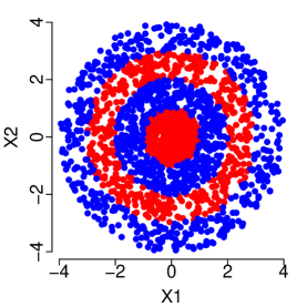
Figure 1: Scatter plot of 2000 observations (1000 from each class) from the two classes in Example 1 with $d=2$. Red (respectively, blue) represents observations from Class-1 (respectively, Class-2).

A scatter plot of this dataset for $d=2$ is shown in Figure 1. We consider this example with $d=2,4$ and $6$, and in each case, we form training and test sets of sizes $200$ and $10,000$, respectively, taking an equal number of observations from the two classes. We repeat the data generation $100$ times and compute the average empirical misclassification rates of several popular parametric and nonparametric classifiers on the test data, which are reported in Table 1. In this example, the competing classes have disjoint supports, so the Bayes risk is zero. But, the Bayes classifier is highly non-linear. So, as expected, linear discriminant analysis (LDA, e.g., Anderson, 2009) and other linear classifiers like logistic regression, GLMNET (see, e.g., Friedman et al., 2010) and linear support vector machines (SVM, e.g., Duda et al., 2007) have misclassification rates close to 50%. Performances of quadratic discriminant analysis (QDA, e.g., Anderson, 2009) and nonparametric classifiers like the $k$-nearest neighbour classifier ($k$NN, e.g., Cover and Hart, 1967), kernel discriminant analysis (KDA, e.g., Hand, 1982), classification tree (CART, e.g., Breiman et al., 2017) and random forest (Breiman, 2001) are only marginally better. All these state-of-the-art classifiers fail to yield satisfactory performance. Nonlinear SVM with radial basis function kernel (see, e.g. Cristianini and Shawe-Taylor, 2003; Schölkopf and Smola, 2002) has somewhat better performance, but even this classifier has misclassification rates close to 36% for $d=4$ and $d=6$. Apart from the curse of dimensionality, one major drawback of the nonparametric methods is that even if we have some structural information about the underlying distributions, that useful information cannot be utilized during the construction of the classification rule. If we can extract that information and use it judiciously, the resulting classifier can have improved performance. It is known that for elliptic distributions, MD carries substantial information about the density. Keeping that in mind, we construct a classifier based on MD that leverages the underlying structural information (details given in the next section). This classifier (henceforth, referred to as the MD classifier) does not involve any density estimation, but still can be viewed as a generalization of LDA and QDA. The proposed classifier has excellent performance in Example 1, where it outperforms all other classifiers. In particular, for $d=4$ and $6$, while all other classifiers have misclassification rates higher than 30%, the misclassification rates of the MD classifier are less than 10%.

$d$	LDA	QDA	Logistic	GLM	Neural	$k$NN	KDA	CART	Random	SVM	SVM	MD
				Net	Net				Forest	Linear	RBF	(proposed)
$2$	49.58	41.92	49.59	49.57	43.47	12.75	19.71	28.86	14.22	45.09	7.84	6.85
	$\scriptstyle(0.11)$	$\scriptstyle(0.25)$	$\scriptstyle(0.11)$	$\scriptstyle(0.11)$	$\scriptstyle(0.17)$	$\scriptstyle(0.20)$	$\scriptstyle(0.23)$	$\scriptstyle(0.43)$	$\scriptstyle(0.21)$	$\scriptstyle(0.12)$	$\scriptstyle(0.13)$	$\scriptstyle(0.27)$
$4$	49.43	42.11	49.45	49.37	44.42	32.80	36.72	38.85	33.08	46.39	33.44	7.75
	$\scriptstyle(0.10)$	$\scriptstyle(0.14)$	$\scriptstyle(0.10)$	$\scriptstyle(0.10)$	$\scriptstyle(0.09)$	$\scriptstyle(0.31)$	$\scriptstyle(0.24)$	$\scriptstyle(0.26)$	$\scriptstyle(0.12)$	$\scriptstyle(0.18)$	$\scriptstyle(0.23)$	$\scriptstyle(0.18)$
$6$	49.12	42.29	49.16	49.17	44.86	39.56	41.41	39.84	34.64	46.55	36.98	8.46
	$\scriptstyle(0.11)$	$\scriptstyle(0.12)$	$\scriptstyle(0.11)$	$\scriptstyle(0.11)$	$\scriptstyle(0.11)$	$\scriptstyle(0.19)$	$\scriptstyle(0.20)$	$\scriptstyle(0.25)$	$\scriptstyle(0.12)$	$\scriptstyle(0.17)$	$\scriptstyle(0.16)$	$\scriptstyle(0.18)$

Boldface character signifies the best result in each case.

Table 1: Average misclassification rates (in %) of different classifiers in Example 1 for varying choices of $d$. The standard errors are reported in the next line within brackets in a smaller font.

The description of the MD classifier is given in the next section, and a few other simulated datasets involving elliptic distributions are analyzed to evaluate its performance. However, when the underlying distributions are non-elliptic, in particular, if they are multimodal in nature, the MD classifier may not work well. To take care of this problem, we propose a local version of MD and develop a classifier based on those local distances. The description of this classifier is given in Section 3. This local Mahalanobis distance (LMD) involves a tuning parameter that controls the degree of localization. For higher values of this parameter, local Mahalanobis distances behave like usual Mahalanobis distances, and the classifier behaves like the MD classifier. But, for smaller values of the tuning parameter, it performs like the nonparametric methods. So, for a suitable choice of this parameter, the proposed method can perform well both for elliptic and non-elliptic distributions. We use the bootstrap method to select this parameter and investigate the performance of the resulting classifier on several simulated datasets. In Section 4, we study the high-dimensional behaviour of our proposed classifiers and observe that unlike many popular nonparametric classifiers, our proposed methods can perform well even in high dimension, low sample size (HDLSS) situations. Some benchmark datasets are analyzed in Section 5 to compare the performance of the proposed classifiers with some state-of-the-art classifiers. Section 6 contains a brief summary of the work and ends with a discussion on related issues. All proofs and mathematical details are given in the Appendix.

2 Classifier based on Mahalanobis distances

Consider a $J$-class classification problem, where the $j$-th class ($j=1,2,\ldots,J$) has probability density function $f_{j}$ with location $\bm{\mu}_{j}$ and scatter matrix $\bm{\Sigma}_{j}$. For any observation $\mathbf{x}$, its Mahalanobis distance from the $j$-th class is given by $\delta_{j}({\bf x})=\{({\bf x}-\mbox{\boldmath$\mu$}_{j})^{\top}\mbox{\boldmath$\Sigma$}_{j}^{-1}({\bf x}-\mbox{\boldmath$\mu$}_{j})\}^{1/2}$, where $\mathbf{a}^{\top}$ denotes the transpose of the vector $\mathbf{a}$. Note that if $f_{j}$ is the density of an elliptically symmetric distribution (see, e.g., Fang et al., 2018), then its form is given by

$$f_{j}({\bf x})=C_{j}|\mbox{\boldmath$\Sigma$}_{j}|^{-1/2}\phi_{j}(\delta_{j}({\bf x})),$$

where $|\mbox{\boldmath$\Sigma$}_{j}|$ is the determinant of $\mbox{\boldmath$\Sigma$}_{j}$, $C_{j}$ is a positive constant, and $\phi_{j}:{\mathbb{R}}_{+}\rightarrow{\mathbb{R}}_{+}$ is a non-negative function. Therefore, if the competing classes are elliptically symmetric and $\pi_{j}$ is the prior probability of the $j$-th class, then the logarithm of the ratio of the posterior probabilities of the $j$-th and the $j^{\prime}$-th classes ($1\leq j\neq j^{\prime}\leq J$) can be expressed as

$$\log\left(\frac{p(j\mid\mathbf{x})}{p(j^{\prime}\mid\mathbf{x})}\right)=(\alpha_{j}-\alpha_{j^{\prime}})+\psi_{j}(\delta_{j}({\bf x}))-\psi_{j^{\prime}}(\delta_{j^{\prime}}({\bf x})),$$

where $\psi_{j}(t)=\log(\phi_{j}(t))$ and $\alpha_{j}=\log(C_{j}\pi_{j}|\mbox{\boldmath$\Sigma$}|^{-1/2}_{j})$. So, the posterior probabilities of different classes follow a generalized additive model (GAM, e.g., Hastie and Tibshirani, 1990; Wood, 2017) with the logistic link function involving Mahalanobis distances $\Delta({\bf x})=(\delta_{1}({\bf x}),\ldots,\delta_{J}({\bf x}))$ as the covariates. We state this as a theorem below.

Theorem 2.1.

If the densities of $J$ competing classes are elliptically symmetric, their posterior probabilities satisfy an additive logistic regression model given by

$$p(j\mid\mathbf{x})=\frac{\exp\Big{(}g_{j}\big{(}\Delta(\mathbf{x})\big{)}\Big{)}}{1+\sum_{k=1}^{J-1}\exp\Big{(}g_{k}\big{(}\Delta(\mathbf{x})\big{)}\Big{)}}\text{ for }j=1,\ldots,J-1\text{ and }p(J\mid{\bf x})=\frac{1}{1+\sum_{k=1}^{J-1}\exp\Big{(}g_{k}\big{(}\Delta(\mathbf{x})\big{)}\Big{)}},$$

where $g_{j}\big{(}\Delta({\bf x})\big{)}=\sum_{k=1}^{J}g_{jk}\big{(}\delta_{k}({\bf x})\big{)}$ is an additive function of $\Delta(\mathbf{x})=\big{(}\delta_{1}(\mathbf{x}),\ldots,\delta_{J}(\mathbf{x})\big{)}$.

Motivated by the above result, for constructing a classifier, we start by estimating the empirical Mahalanobis distances from the training data $\{{\bf x}_{ji}:~{}j=1,\ldots,J,~{}i=1,\ldots,n_{j}\}$, where ${\bf x}_{ji}$ denotes the $i$-th observation from the $j$-th class. We use this dataset to estimate the location vectors and scatter matrices of different classes. Usually, one uses moment-based estimates, but robust estimates like minimum covariance determinant (MCD, e.g., Rousseeuw and Driessen, 1999) or minimum volume ellipsoid (MVE, e.g., Van Aelst and Rousseeuw, 2009) can also be used. After getting these estimates ${\widehat{}\mbox{\boldmath$\mu$}}_{j}$ and ${\widehat{}\mbox{\boldmath$\Sigma$}}_{j}$ for $j=1,\ldots,J$, for each ${\bf x}_{ji}$, we estimate the vector of Mahalanobis distances by ${\widehat{\Delta}}({\bf x}_{ji})=\big{(}\widehat{\delta}_{1}({\bf x}_{ji}),\ldots,{\widehat{\delta}_{J}}({\bf x}_{ji})\big{)}$, where ${\widehat{\delta}}_{j}({\bf x})=\big{\{}({\bf x}-{\widehat{}\mbox{\boldmath$\mu$}}_{j})^{\top}{\widehat{}\mbox{\boldmath$\Sigma$}}_{j}^{-1}({\bf x}-{\widehat{}\mbox{\boldmath$\mu$}}_{j})\big{\}}^{1/2}$ for $j=1,\ldots,J$. Pointwise convergence of $\widehat{\delta}_{j}$ to $\delta_{j}$ follows from the convergence of $\widehat{}\mbox{\boldmath$\mu$}_{j}$ and $\widehat{}\mbox{\boldmath$\Sigma$}_{j}$ to their population counterparts. In fact, uniform convergence of $\widehat{\delta}_{j}$ over any compact set holds for consistent estimators $\widehat{}\mbox{\boldmath$\mu$}_{j}$ and $\widehat{}\mbox{\boldmath$\Sigma$}_{j}$ of $\mu$ and $\Sigma$, respectively. This follows from the result given below.

Lemma 2.1.

Let $\mathbf{X}_{1},\ldots,\mathbf{X}_{n}$ be i.i.d. copies of $\mathbf{X}\in\mathbb{R}^{d}$, which has finite second moments. Define $\mbox{\boldmath$\mu$}=\mathbb{E}(\mathbf{X})$ and $\mbox{\boldmath$\Sigma$}=\mathbb{V}\mathrm{ar}(\mathbf{X})$, and suppose that $\Sigma$ is positive definite. Let $\widehat{}\mbox{\boldmath$\mu$}$ and $\widehat{}\mbox{\boldmath$\Sigma$}^{-1}$ be $\sqrt{n}$-consistent estimators of $\mu$ and $\mbox{\boldmath$\Sigma$}^{-1}$, respectively, i.e., $\|\widehat{}\mbox{\boldmath$\mu$}-\mbox{\boldmath$\mu$}\|=O_{\mathbb{P}}(n^{-1/2})$ and $\|\widehat{}\mbox{\boldmath$\Sigma$}^{-1}\mkern-10.0mu-\mbox{\boldmath$\Sigma$}^{-1}\|_{\rm F}=O_{\mathbb{P}}(n^{-1/2})$, where $\|\cdot\|_{\rm F}$ is the Frobenius norm. Then, for any compact set $\mathcal{C}\subset\mathbb{R}^{d}$, we have

$$\sup_{\mathbf{x}\in\mathcal{C}}\left\|(\mathbf{x}-\widehat{}\mbox{\boldmath$\mu$})^{\top}\widehat{}\mbox{\boldmath$\Sigma$}^{-1}(\mathbf{x}-\widehat{}\mbox{\boldmath$\mu$})-(\mathbf{x}-\mbox{\boldmath$\mu$})^{\top}\mbox{\boldmath$\Sigma$}^{-1}(\mathbf{x}-\mbox{\boldmath$\mu$})\right\|=O_{\mathbb{P}}(n^{-1/2}).$$

Remark 1.

The assumption of $\mathbf{X}$ having finite second moment in Lemma 2.1 is not necessary. The same proof holds with $\mu$ and $\Sigma$ being the location vector and scatter matrix (not necessarily moment based), as long as we can find $\sqrt{n}$-consistent estimators for $\mu$ and $\mbox{\boldmath$\Sigma$}^{-1}$. Moreover, if we have consistent estimators but of different rates of convergence, then also the result follows. In this case, the uniform rate of convergence will be the slower of the two convergence rates (of $\widehat{}\mbox{\boldmath$\mu$}$ and $\widehat{}\mbox{\boldmath$\Sigma$}^{-1}$).

In the case of a high-dimensional problem, the MDs $\widehat{\Delta}(\mathbf{x}_{ji})$ can provide a low-dimensional view of the class separability. This visualization is particularly useful in binary classification. To demonstrate this, we show in Figure 2 the scatter plot of the ${\widehat{\Delta}}({\bf x}_{ji})$’s for the binary classification problem in Example 1 with $d=4$ and $d=6$. The separability of the two classes is clearly visible from this figure.

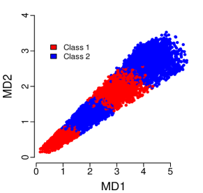
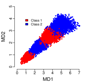
Figure 2: Scatter plot of estimated Mahalanobis distances in Example 1 for $d=4$ (left) and $d=6$ (right).

Motivated by Theorem 2.1, we use the $\widehat{\Delta}(\mathbf{x}_{ji})$’s as extracted features and fit a GAM to get estimates of the additive functions $\widehat{g}_{1},\ldots,\widehat{g}_{J}$, and subsequently, the posterior probabilities $\widehat{p}(1\mid\mathbf{x}),\ldots,\widehat{p}(J\mid\mathbf{x})$. Finally, an observation $\mathbf{x}$ is assigned to the class having the highest estimated posterior. We have already seen that this classifier has excellent performance in Example 1. In the next subsection, we evaluate its empirical performance on some more simulated datasets.

2.1 Empirical Performance of the MD classifier

Here, we consider some classification problems involving two or more elliptic distributions. For all the examples, we form the training set by generating 100 observations from each class, while 1000 (5000 for two-class problems) observations from each class are generated to form the test set. Each experiment is repeated 100 times to compute the average test set misclassification errors and the corresponding standard errors of different classifiers. These results are reported in Table 2 for $d=2,4$ and $6$. Like Example 1, here also we compare the performance of the MD classifier with some popular classifiers. Some of these competing classifiers involve tuning parameters, which are chosen using 5-fold cross-validation. All classification methods are implemented using R codes.

Example 2.

We consider two multivariate normal distributions $N_{d}({-0.3}{\bf 1}_{d},{\bf I}_{d})$ and $N_{d}({0.3}{\bf 1}_{d},{\bf I}_{d})$ differing only in their locations. Here, ${\bf 1}_{d}$ denotes the $d$-dimensional vector with all elements equal to $1$, and ${\bf I}_{d}$ denotes the $d\times d$ identity matrix.

Here, the Bayes classifier is linear. In fact, this is an ideal setup for LDA to perform well. So, as expected, LDA has the lowest misclassification rate in this example, and all linear classifiers perform better than nonlinear classifiers. Nevertheless, all the classifiers have satisfactory performance.

Example 3.

We consider two multivariate normal distributions $N_{d}({\bf 0}_{d},{\bf I}_{d})$ and $N_{d}({\bf 0}_{d},5{\bf I}_{d})$, which differ only in their scales. Here, ${\bf 0}_{d}$ is the $d$-dimensional vector with all elements equal to $0$.

In this example, the Bayes classifier is a quadratic function, and this setup is ideal for QDA. So, QDA has the best performance here. The MD classifier has the second-best performance, closely followed by the nonlinear SVM. Among the others, Random Forest has a somewhat satisfactory performance. The rest of the classifiers perform very poorly.

Example 4.

Consider two elliptical distributions, one of which is $U_{d,\mbox{\boldmath$\Sigma$}}(1,2)$ and the other one is an equal mixture of $U_{d,\mbox{\boldmath$\Sigma$}}(0,1)$ and $U_{d,\mbox{\boldmath$\Sigma$}}(2,3)$. Here, $U_{d,\mbox{\boldmath$\Sigma$}}(a,b)$ denotes the $d$-dimensional uniform distribution over the region $\{{\bf x}\in{\mathbb{R}}^{d}:a\leq\|\mbox{\boldmath$\Sigma$}^{1/2}{\bf x}\|\leq b\}$. The matrix $\Sigma$ has all diagonal elements equal to $1$ and all off-diagonal elements equal to $0.5$.

Like Example 1, here also the MD classifier performs much better than its competitors. While it has misclassification rates close to 5%, all other competing methods have much higher misclassification rates, especially for $d=4$ and $d=6$.

Data	$d$	Bayes	LDA	QDA	Logist	GLM	Neural	$k$NN	KDA	CART	Rand	SVM	SVM	MD
set					Reg.	Net	Net				Forest	Linear	Nonlin	Class
	2	33.53	33.89	34.18	33.89	34.39	34.25	35.71	35.12	38.08	39.42	33.93	36.11	35.14
		$\scriptstyle(0.05)$	$\scriptstyle(0.07)$	$\scriptstyle(0.08)$	$\scriptstyle(0.07)$	$\scriptstyle(0.14)$	$\scriptstyle(0.11)$	$\scriptstyle(0.22)$	$\scriptstyle(0.29)$	$\scriptstyle(0.24)$	$\scriptstyle(0.17)$	$\scriptstyle(0.06)$	$\scriptstyle(0.29)$	$\scriptstyle(0.15)$
Ex 2	4	27.48	28.09	28.97	28.10	28.50	28.57	29.27	28.93	34.92	31.29	28.13	29.36	29.59
($J=2$)		$\scriptstyle(0.04)$	$\scriptstyle(0.06)$	$\scriptstyle(0.08)$	$\scriptstyle(0.06)$	$\scriptstyle(0.10)$	$\scriptstyle(0.10)$	$\scriptstyle(0.12)$	$\scriptstyle(0.16)$	$\scriptstyle(0.21)$	$\scriptstyle(0.11)$	$\scriptstyle(0.06)$	$\scriptstyle(0.20)$	$\scriptstyle(0.10)$
	6	23.14	24.02	25.47	24.08	24.64	24.76	25.32	24.74	34.16	26.84	24.14	24.77	26.00
		$\scriptstyle(0.05)$	$\scriptstyle(0.07)$	$\scriptstyle(0.10)$	$\scriptstyle(0.07)$	$\scriptstyle(0.12)$	$\scriptstyle(0.11)$	$\scriptstyle(0.11)$	$\scriptstyle(0.11)$	$\scriptstyle(0.20)$	$\scriptstyle(0.10)$	$\scriptstyle(0.07)$	$\scriptstyle(0.11)$	$\scriptstyle(0.11)$
	2	30.74	49.26	31.34	49.27	49.36	44.02	35.45	34.35	35.53	36.44	45.00	33.13	31.80
		$\scriptstyle(0.04)$	$\scriptstyle(0.10)$	$\scriptstyle(0.05)$	$\scriptstyle(0.10)$	$\scriptstyle(0.10)$	$\scriptstyle(0.15)$	$\scriptstyle(0.19)$	$\scriptstyle(0.19)$	$\scriptstyle(0.20)$	$\scriptstyle(0.14)$	$\scriptstyle(0.11)$	$\scriptstyle(0.20)$	$\scriptstyle(0.09)$
Ex 3	4	22.99	49.23	24.35	49.25	49.27	44.03	33.98	32.27	34.33	29.06	45.91	25.74	24.63
($J=2$)		$\scriptstyle(0.04)$	$\scriptstyle(0.09)$	$\scriptstyle(0.06)$	$\scriptstyle(0.09)$	$\scriptstyle(0.10)$	$\scriptstyle(0.11)$	$\scriptstyle(0.17)$	$\scriptstyle(0.17)$	$\scriptstyle(0.24)$	$\scriptstyle(0.13)$	$\scriptstyle(0.12)$	$\scriptstyle(0.11)$	$\scriptstyle(0.09)$
	6	17.90	49.00	19.89	49.03	49.12	44.01	34.24	32.85	33.66	25.32	45.68	21.65	20.09
		$\scriptstyle(0.04)$	$\scriptstyle(0.10)$	$\scriptstyle(0.07)$	$\scriptstyle(0.10)$	$\scriptstyle(0.10)$	$\scriptstyle(0.11)$	$\scriptstyle(0.16)$	$\scriptstyle(0.14)$	$\scriptstyle(0.23)$	$\scriptstyle(0.14)$	$\scriptstyle(0.11)$	$\scriptstyle(0.13)$	$\scriptstyle(0.11)$
	2	0.00	50.32	48.67	50.31	50.27	45.89	9.49	8.42	20.93	10.56	53.04	5.82	4.72
		$\scriptstyle(0.00)$	$\scriptstyle(0.08)$	$\scriptstyle(0.50)$	$\scriptstyle(0.08)$	$\scriptstyle(0.08)$	$\scriptstyle(0.12)$	$\scriptstyle(0.16)$	$\scriptstyle(0.12)$	$\scriptstyle(0.29)$	$\scriptstyle(0.14)$	$\scriptstyle(0.08)$	$\scriptstyle(0.11)$	$\scriptstyle(0.24)$
Ex 4	4	0.00	50.11	51.29	50.10	50.11	48.09	25.30	31.40	38.69	25.84	51.26	16.60	5.18
($J=2$)		$\scriptstyle(0.00)$	$\scriptstyle(0.07)$	$\scriptstyle(0.33)$	$\scriptstyle(0.07)$	$\scriptstyle(0.08)$	$\scriptstyle(0.13)$	$\scriptstyle(0.21)$	$\scriptstyle(0.29)$	$\scriptstyle(0.39)$	$\scriptstyle(0.18)$	$\scriptstyle(0.11)$	$\scriptstyle(0.19)$	$\scriptstyle(0.14)$
	6	0.00	50.02	52.77	50.01	50.00	48.47	32.95	40.93	42.53	31.04	50.80	25.61	4.80
		$\scriptstyle(0.00)$	$\scriptstyle(0.07)$	$\scriptstyle(0.26)$	$\scriptstyle(0.07)$	$\scriptstyle(0.07)$	$\scriptstyle(0.11)$	$\scriptstyle(0.21)$	$\scriptstyle(0.37)$	$\scriptstyle(0.25)$	$\scriptstyle(0.21)$	$\scriptstyle(0.11)$	$\scriptstyle(0.22)$	$\scriptstyle(0.15)$
	2	36.17	49.92	45.72	49.89	49.89	46.37	41.79	42.05	42.80	43.36	49.73	40.02	37.82
		$\scriptstyle(0.04)$	$\scriptstyle(0.11)$	$\scriptstyle(0.59)$	$\scriptstyle(0.11)$	$\scriptstyle(0.10)$	$\scriptstyle(0.14)$	$\scriptstyle(0.21)$	$\scriptstyle(0.25)$	$\scriptstyle(0.24)$	$\scriptstyle(0.14)$	$\scriptstyle(0.26)$	$\scriptstyle(0.26)$	$\scriptstyle(0.13)$
Ex 5	4	30.48	50.02	43.41	49.98	49.95	46.27	39.86	40.08	41.12	37.85	48.96	34.83	32.87
($J=2$)		$\scriptstyle(0.05)$	$\scriptstyle(0.10)$	$\scriptstyle(0.67)$	$\scriptstyle(0.10)$	$\scriptstyle(0.09)$	$\scriptstyle(0.10)$	$\scriptstyle(0.16)$	$\scriptstyle(0.30)$	$\scriptstyle(0.24)$	$\scriptstyle(0.15)$	$\scriptstyle(0.21)$	$\scriptstyle(0.22)$	$\scriptstyle(0.14)$
	6	27.19	49.94	41.40	49.90	49.89	46.42	39.79	40.49	41.10	35.30	48.68	32.58	30.95
		$\scriptstyle(0.04)$	$\scriptstyle(0.10)$	$\scriptstyle(0.67)$	$\scriptstyle(0.10)$	$\scriptstyle(0.10)$	$\scriptstyle(0.12)$	$\scriptstyle(0.12)$	$\scriptstyle(0.41)$	$\scriptstyle(0.26)$	$\scriptstyle(0.13)$	$\scriptstyle(0.17)$	$\scriptstyle(0.23)$	$\scriptstyle(0.17)$
	2	47.32	66.70	66.47	66.68	66.71	64.68	56.44	55.83	58.88	57.62	69.01	54.87	51.65
		$\scriptstyle(0.08)$	$\scriptstyle(0.24)$	$\scriptstyle(0.30)$	$\scriptstyle(0.24)$	$\scriptstyle(0.22)$	$\scriptstyle(0.15)$	$\scriptstyle(0.19)$	$\scriptstyle(0.23)$	$\scriptstyle(0.22)$	$\scriptstyle(0.12)$	$\scriptstyle(0.19)$	$\scriptstyle(0.20)$	$\scriptstyle(0.13)$
Ex 6	4	47.51	66.39	66.09	66.41	66.46	64.64	59.23	59.43	61.30	59.19	67.69	58.00	53.07
($J=3$)		$\scriptstyle(0.07)$	$\scriptstyle(0.24)$	$\scriptstyle(0.31)$	$\scriptstyle(0.24)$	$\scriptstyle(0.22)$	$\scriptstyle(0.15)$	$\scriptstyle(0.12)$	$\scriptstyle(0.14)$	$\scriptstyle(0.16)$	$\scriptstyle(0.12)$	$\scriptstyle(0.23)$	$\scriptstyle(0.17)$	$\scriptstyle(0.13)$
	6	47.29	66.41	65.95	66.35	66.35	64.29	60.56	61.02	62.13	59.40	67.17	59.40	53.83
		$\scriptstyle(0.08)$	$\scriptstyle(0.22)$	$\scriptstyle(0.29)$	$\scriptstyle(0.22)$	$\scriptstyle(0.22)$	$\scriptstyle(0.14)$	$\scriptstyle(0.12)$	$\scriptstyle(0.20)$	$\scriptstyle(0.16)$	$\scriptstyle(0.10)$	$\scriptstyle(0.24)$	$\scriptstyle(0.14)$	$\scriptstyle(0.13)$
	2	44.77	65.16	45.71	65.17	65.27	60.26	50.61	52.40	56.18	53.41	61.87	48.53	46.52
		$\scriptstyle(0.08)$	$\scriptstyle(0.32)$	$\scriptstyle(0.10)$	$\scriptstyle(0.32)$	$\scriptstyle(0.31)$	$\scriptstyle(0.42)$	$\scriptstyle(0.16)$	$\scriptstyle(0.29)$	$\scriptstyle(0.26)$	$\scriptstyle(0.13)$	$\scriptstyle(0.42)$	$\scriptstyle(0.14)$	$\scriptstyle(0.11)$
Ex 7	4	29.68	63.85	31.52	63.87	63.81	59.41	41.97	44.80	50.46	39.04	57.77	36.48	32.32
($J=3$)		$\scriptstyle(0.07)$	$\scriptstyle(0.28)$	$\scriptstyle(0.11)$	$\scriptstyle(0.28)$	$\scriptstyle(0.28)$	$\scriptstyle(0.33)$	$\scriptstyle(0.14)$	$\scriptstyle(0.09)$	$\scriptstyle(0.28)$	$\scriptstyle(0.15)$	$\scriptstyle(0.48)$	$\scriptstyle(0.14)$	$\scriptstyle(0.12)$
	6	23.24	62.68	25.96	62.73	62.91	58.33	40.05	43.43	49.26	34.07	56.05	31.64	26.82
		$\scriptstyle(0.08)$	$\scriptstyle(0.26)$	$\scriptstyle(0.11)$	$\scriptstyle(0.26)$	$\scriptstyle(0.28)$	$\scriptstyle(0.27)$	$\scriptstyle(0.16)$	$\scriptstyle(0.10)$	$\scriptstyle(0.31)$	$\scriptstyle(0.13)$	$\scriptstyle(0.41)$	$\scriptstyle(0.17)$	$\scriptstyle(0.12)$
	2	33.60	49.85	41.20	47.82	47.64	44.24	40.37	37.72	38.72	39.33	48.03	37.49	35.01
		$\scriptstyle(0.04)$	$\scriptstyle(0.06)$	$\scriptstyle(0.39)$	$\scriptstyle(0.14)$	$\scriptstyle(0.17)$	$\scriptstyle(0.10)$	$\scriptstyle(0.16)$	$\scriptstyle(0.18)$	$\scriptstyle(0.24)$	$\scriptstyle(0.10)$	$\scriptstyle(0.16)$	$\scriptstyle(0.21)$	$\scriptstyle(0.09)$
Ex 8	4	28.72	49.85	44.86	47.94	47.51	44.24	40.80	37.41	38.82	35.46	46.80	33.81	30.50
($J=2$)		$\scriptstyle(0.05)$	$\scriptstyle(0.06)$	$\scriptstyle(0.52)$	$\scriptstyle(0.12)$	$\scriptstyle(0.14)$	$\scriptstyle(0.10)$	$\scriptstyle(0.21)$	$\scriptstyle(0.18)$	$\scriptstyle(0.25)$	$\scriptstyle(0.12)$	$\scriptstyle(0.20)$	$\scriptstyle(0.23)$	$\scriptstyle(0.13)$
	6	25.54	49.79	47.46	48.08	47.28	44.47	41.49	38.70	38.43	33.59	46.04	32.88	28.30
		$\scriptstyle(0.04)$	$\scriptstyle(0.07)$	$\scriptstyle(0.29)$	$\scriptstyle(0.10)$	$\scriptstyle(0.15)$	$\scriptstyle(0.14)$	$\scriptstyle(0.23)$	$\scriptstyle(0.20)$	$\scriptstyle(0.23)$	$\scriptstyle(0.14)$	$\scriptstyle(0.19)$	$\scriptstyle(0.29)$	$\scriptstyle(0.29)$

Boldface character signifies the best result in each case.

Table 2: Average misclassification rates (in %) of different classifiers in Examples 2–8 for varying $d$. The corresponding standard errors are reported in the next line within brackets in a smaller font.

Example 5.

The underlying distributions of the two competing classes are $N_{d}({\bf 0}_{d},3{\bf I}_{d})$ and the standard multivariate $t$ distribution with $3$ degrees of freedom.

These two distributions have the same locations and covariance matrices, while their shapes are different. In this example, the MD classifier outperforms all other classifiers. Only nonlinear SVM and Random Forest have somewhat competitive performances.

Example 6.

We consider three spherical distributions (see, e.g., Fang et al., 2018). A spherical distribution is completely specified by the distribution of its radius $R$. The radius $R$ follows the uniform distribution $U(0,10)$ for Class-1 and the normal distribution $N(5.5,\sigma^{2})$ for Class-2. For Class-3, it is distributed as $cY$, where $Y$ follows a beta distribution with parameters $0.5$ and $0.5$. We choose $\sigma^{2}$ and $c$ in such a way that $\mathbb{E}(R^{2})$ is the same in all three cases.

This is a difficult classification problem, where all competing classes have the same location vector and covariance matrix. So, it is not surprising to see that many classifiers perform like the random classifier and have misclassification rates close to $2/3$. The MD classifier has the lowest misclassification rate. Among the rest, only nonlinear SVM has a somewhat better result.

Example 7.

This is again a three class problem. The classes have normal distributions with the centres at the origin, differing only in their correlation structures. The corresponding covariance matrices have diagonal elements $1$, while all the off-diagonal elements are 0.1, 0.5 and 0.9 for the three classes, respectively.

In this example with normal distributions differing in their covariance structures, as expected, QDA has the best performance. But, the MD classifier closely follows QDA and has much better performance than all other classifiers considered here.

Example 8.

We consider a classification problem between a normal and a Cauchy distribution with the same location ${\bf 0}_{d}$ and the same scatter matrix having all diagonal elements equal to $1$ and all off-diagonal elements equal to $0.1$.

Since the Cauchy distribution does not have finite moments, in this example, we use the MCD estimate (Rousseeuw and Driessen, 1999) of $\Sigma$ (based on 75% observations) to compute the empirical Mahalanobis distances. We use these estimates for LDA and QDA as well. Here also, the MD classifier outperforms its competitors and the difference becomes more prominent as the dimension increases.

3 Classifier Based on Local Mahalanobis Distances

We have seen that the MD classifier performs very well when the underlying class distributions are elliptic. But, when the underlying densities are not elliptic, Mahalanobis distance may fail to extract substantial information about it. Especially, in the case of multimodal distributions, the local nature of the density functions may not be captured well by Mahalanobis distances. As a result, in a classification problem involving non-elliptic distributions, the proposed MD classifier may fail to have satisfactory performance (this is demonstrated later in the paper). To cope with these situations, we define a local version of Mahalanobis distance. To this effect, first note that for any $\mathbf{x}\in\mathbb{R}^{d}$, we have

$$(\mathbf{x}-\mbox{\boldmath$\mu$})^{\top}\mbox{\boldmath$\Sigma$}^{-1}(\mathbf{x}-\mbox{\boldmath$\mu$})=\mathbb{E}\left\{(\mathbf{x}-\mathbf{X})^{\top}\mbox{\boldmath$\Sigma$}^{-1}(\mathbf{x}-\mathbf{X})\right\}-d,$$

where the random vector $\mathbf{X}$ follows a $d$-dimensional distribution with mean $\mu$ and covariance $\Sigma$. Similarly, for a collection of observations $\mathbf{x}_{1},\ldots,\mathbf{x}_{n}$, if we define $\widehat{}\mbox{\boldmath$\mu$}=\bar{\mathbf{x}}=n^{-1}\sum_{i=1}^{n}\mathbf{x}_{i}$ and $\widehat{}\mbox{\boldmath$\Sigma$}=\mathbf{S}=n^{-1}\sum_{i=1}^{n}(\mathbf{x}_{i}-\bar{\mathbf{x}})(\mathbf{x}_{i}-\bar{\mathbf{x}})^{\top}$ to be the moment-based estimators of location and scatter, then

$$(\mathbf{x}-\widehat{}\mbox{\boldmath$\mu$})^{\top}\widehat{}\mbox{\boldmath$\Sigma$}^{-1}(\mathbf{x}-\widehat{}\mbox{\boldmath$\mu$})=\frac{1}{n}\sum_{i=1}^{n}(\mathbf{x}-\mathbf{x}_{i})^{\top}\widehat{}\mbox{\boldmath$\Sigma$}^{-1}(\mathbf{x}-\mathbf{x}_{i})-d.$$

So, working with the squared Mahalanobis distance (respectively, its sample version) is equivalent to working with the location shift version $\mathbb{E}\{(\mathbf{x}-\mathbf{X})^{\top}\mbox{\boldmath$\Sigma$}^{-1}(\mathbf{x}-\mathbf{X})\}$ (respectively, $n^{-1}\sum_{i=1}^{n}(\mathbf{x}-\mathbf{x}_{i})^{\top}\widehat{}\mbox{\boldmath$\Sigma$}^{-1}(\mathbf{x}-\mathbf{x}_{i})$). It is easy to see that additive functions of Mahalanobis distances are also additive functions of the location shift versions of squared Mahalanobis distances, so Theorem 2.1 remains valid for this version as well. Now, for a fixed point $\mathbf{x}$, $\mathbb{E}\{(\mathbf{x}-\mathbf{X})^{\top}\mbox{\boldmath$\Sigma$}^{-1}(\mathbf{x}-\mathbf{X})\}$ puts equal weight on all points $\mathbf{X}$ on the support of the distribution, irrespective of its relative position with respect to $\mathbf{x}$. Similarly, $n^{-1}\sum_{i=1}^{n}(\mathbf{x}-\mathbf{x}_{i})^{\top}\widehat{}\mbox{\boldmath$\Sigma$}^{-1}(\mathbf{x}-\mathbf{x}_{i})$ puts equal weight on all observations $\mathbf{x}_{1},\ldots,\mathbf{x}_{n}$. In order to capture the local nature of the underlying distribution, we need to use a weighted average, giving more weight to the points near $\mathbf{x}$. We achieve this by using the idea of kernel density estimation. Using a kernel function $K:\mathbb{R}^{d}\to\mathbb{R}_{+}$, which is the density function of a $d$-variate spherical distribution symmetric about the origin (i.e., $K(\mathbf{t})=\Psi(\mathbf{t}^{\top}\mathbf{t}),\mathbf{t}\in\mathbb{R}^{d}$ for some decreasing function $\Psi:\mathbb{R}_{+}\to\mathbb{R}_{+}$), we define

$$\beta_{h}(\mathbf{x})= \mathbb{E}\left[K\Big{(}\frac{\mbox{\boldmath$\Sigma$}^{-1/2}(\mathbf{x}-\mathbf{X})}{h}\Big{)}(\mathbf{x}-\mathbf{X})^{\top}{\mbox{\boldmath$\Sigma$}}^{-1}(\mathbf{x}-\mathbf{X})\right]$$

$$= \mathbb{E}\left[\Psi\Big{(}\frac{1}{h^{2}}{(\mathbf{x}-\mathbf{X})^{\top}{\mbox{\boldmath$\Sigma$}}^{-1}(\mathbf{x}-\mathbf{X})}\Big{)}(\mathbf{x}-\mathbf{X})^{\top}{\mbox{\boldmath$\Sigma$}}^{-1}(\mathbf{x}-\mathbf{X})\right]$$

The behaviour of the function $\beta_{h}(\cdot)$ depends on the tuning parameter $h$. We call $h$ the “localization parameter” as it determines the local weighting scheme in the calculation of $\beta_{h}(\cdot)$. The function $\beta_{h}$ exhibits two different behaviors depending on the value of $h$. For large values of $h$, it behaves similar to the Mahalanobis distance. On the other hand, for small values of $h$, it behaves similar to the density of the underlying distribution. The formal result is given below.

Lemma 3.1.

(a) If $K$ is continuous at $\mathbf{0}$, then $\beta_{h}(\mathbf{x})\to K({\bf 0})\{(\mathbf{x}-\mbox{\boldmath$\mu$})^{\top}\mbox{\boldmath$\Sigma$}^{-1}(\mathbf{x}-\mbox{\boldmath$\mu$})+d\}$ as $h\to\infty$.
(b) If $\int(\mathbf{z}^{\top}\mathbf{z})^{2}K(\mathbf{z})\,d\mathbf{z}<\infty$ and the density $f$ of $\mathbf{X}$ is twice differentiable, then $\beta_{h}(\mathbf{x})/h^{d+2}\to|\mbox{\boldmath$\Sigma$}|^{1/2}\kappa_{2}f(\mathbf{x})$ as $h\to 0$, where $\kappa_{2}=\int\mathbf{z}^{\top}\mathbf{z}\,K(\mathbf{z})\,d\mathbf{z}$.

Based on this result, we define the local (squared) Mahalanobis distance (LMD) as

$$\gamma^{h}(\mathbf{x})=\begin{cases}\beta_{h}(\mathbf{x})&\text{if }h>1,\\ \beta_{h}(\mathbf{x})/{h^{d+2}}&\text{if }h\leq 1.\end{cases}$$ (1)

Lemma 3.1 shows that for a small value of $h$, $\gamma^{h}$ contains information about the underlying density function. Hence, it is quite meaningful to use them as features to construct a classification rule. In fact, the Bayes classifier is related to (the limiting value of) $\gamma^{h}$ via a GAM, as shown below.

Theorem 3.1.

In a $J$-class classification problem, if the underlying class distributions are absolutely continuous, then the posterior probabilities satisfy an additive logistic regression model given by

$$p(j\mid\mathbf{x})=\frac{\exp\Big{(}\zeta_{j}\big{(}\Gamma^{0}(\mathbf{x})\big{)}\Big{)}}{1+\sum_{k=1}^{J-1}\exp\Big{(}\zeta_{k}\big{(}\Gamma^{0}(\mathbf{x})\big{)}\Big{)}}\text{ for }j=1,\ldots,J-1\text{ and }p(J\mid\mathbf{x})=\frac{1}{1+\sum_{k=1}^{J-1}\exp\Big{(}\zeta_{k}\big{(}\Gamma^{0}(\mathbf{x})\big{)}\Big{)}},$$

where $\zeta_{j}\big{(}\Gamma^{0}(\mathbf{x})\big{)}=\sum_{k=1}^{J}\zeta_{jk}\big{(}\gamma^{0}_{k}(\mathbf{x})\big{)}$ is an additive function of $\Gamma^{0}(\mathbf{x})=\big{(}\gamma^{0}_{1}(\mathbf{x}),\ldots,\gamma^{0}_{J}(\mathbf{x})\big{)}$, and $\gamma^{0}_{j}(\mathbf{x})=\lim_{h\downarrow 0}\gamma_{j}^{h}(\mathbf{x})$ for $j=1,2,\ldots,J$.

So, instead of MD, one can use LMD (with a suitable choice of $h$) as features and construct a classifier using GAM as before. In practice, we compute the estimates $\widehat{}\mbox{\boldmath$\Sigma$}_{1},\ldots,\widehat{}\mbox{\boldmath$\Sigma$}_{J}$ from the data and compute

$$\widehat{\beta}_{h,j}(\mathbf{x}) =\frac{1}{n_{j}}\sum_{i=1}^{n_{j}}\left\{K\bigg{(}\frac{\widehat{}\mbox{\boldmath$\Sigma$}_{j}^{-1/2}(\mathbf{x}-\mathbf{x}_{ji})}{h}\bigg{)}(\mathbf{x}-\mathbf{x}_{ji})^{\top}{\widehat{}\mbox{\boldmath$\Sigma$}}_{j}^{-1}(\mathbf{x}-\mathbf{x}_{ji})\right\}$$

$$=\frac{1}{n_{j}}\sum_{i=1}^{n_{j}}\left\{\Psi\bigg{(}\frac{1}{h^{2}}{(\mathbf{x}-\mathbf{x}_{ji})^{\top}{\widehat{}\mbox{\boldmath$\Sigma$}}_{j}^{-1}(\mathbf{x}-\mathbf{x}_{ji})}\bigg{)}(\mathbf{x}-\mathbf{x}_{ji})^{\top}{\widehat{}\mbox{\boldmath$\Sigma$}}_{j}^{-1}(\mathbf{x}-\mathbf{x}_{ji})\right\},\qquad j=1,2,\ldots,J.$$

Estimates of the LMDs are obtained using the formula

$$\widehat{\gamma}_{j}^{h}(\mathbf{x})=\begin{cases}\widehat{\beta}_{h,j}(\mathbf{x})&\text{if }h>1,\\ \widehat{\beta}_{h,j}(\mathbf{x})/{h^{d+2}}&\text{if }h\leq 1.\end{cases}$$ (2)

For the empirical version of LMD, we have uniform convergence result similar to Lemma 2.1 if the function $\Psi$ is bounded and Lipschitz continuous. The result is stated below.

Lemma 3.2.

Let $\mathbf{X}_{1},\ldots,\mathbf{X}_{n}$ be i.i.d. copies of $\mathbf{X}\in\mathbb{R}^{d}$, which has finite fourth moments. Let $\gamma^{h}(\cdot)$ be the LMD as defined in (1) and $\widehat{\gamma}^{h}(\cdot)$ be its empirical version as defined in (2), based on $\mathbf{X}_{1},\ldots,\mathbf{X}_{n}$. Suppose that the function $\Psi$ is bounded and Lipschitz continuous, and $\widehat{}\mbox{\boldmath$\Sigma$}^{-1}$ is a $\sqrt{n}$-consistent estimator of $\mbox{\boldmath$\Sigma$}^{-1}$, i.e., $\|\widehat{}\mbox{\boldmath$\Sigma$}^{-1}\mkern-10.0mu-\mbox{\boldmath$\Sigma$}^{-1}\|_{\rm F}=O_{\mathbb{P}}(n^{-1/2})$. Then, for any fixed $h>0$ and any compact set $\mathcal{C}\subset\mathbb{R}^{d}$, we have $\sup_{\mathbf{x}\in\mathcal{C}}\big{|}\widehat{\gamma}^{h}(\mathbf{x})-\gamma^{h}(\mathbf{x})\big{|}=O_{\mathbb{P}}(n^{-1/2})$.

Note that if we use the Gaussian kernel (i.e., $K(\mathbf{t})=(2\pi)^{-d/2}e^{-(\mathbf{t}^{\top}\mathbf{t})/2}$), then the corresponding function $\Psi(t)=(2\pi)^{-d/2}e^{-t^{2}/2}$ satisfies the properties mentioned in the lemma above. Also, although we have proved the lemma for a fixed $h$, from the proof it is easy to see that the same result holds for a sequence $\{h_{n}\}$ that is uniformly bounded away from $0$. That is, if $\{h_{n}\}$ is a sequence of real numbers satisfying $\inf_{n\geq 1}h_{n}\geq h_{0}$ for some $h_{0}>0$, then $\sup_{\mathbf{x}\in\mathcal{C}}|\widehat{\gamma}^{h_{n}}(\mathbf{x})-\gamma^{h_{n}}(\mathbf{x})|=O_{\mathbb{P}}(n^{-1/2})$. So, the estimated LMD is close to its population counterpart for arbitrarily large $h$, which in turn behaves like the shifted squared Mahalanobis distance. The case of small $h$, however, is more tricky. For a general sequence $\{h_{n}\}$, we have $\sup_{\mathbf{x}\in\mathcal{C}}|\widehat{\gamma}^{h_{n}}(\mathbf{x})-\gamma^{h_{n}}(\mathbf{x})|=O_{\mathbb{P}}\big{(}n^{-1/2}h_{n}^{-(d+2)}\wedge n^{-1/2}h_{n}^{-(d+4)}\big{)}$. Thus, for $h_{n}\to 0$, we have the uniform convergence $\sup_{\mathbf{x}\in\mathcal{C}}|\widehat{\gamma}^{h_{n}}(\mathbf{x})-\gamma^{h_{n}}(\mathbf{x})|\overset{\mathbb{P}}{\to}0$ as $n\to\infty$ if $\sqrt{n}h_{n}^{d+4}\to\infty$. So, we cannot use an arbitrarily small value of $h$ in practice. It should decrease at an appropriate rate as the sample size increases.

To demonstrate the empirical behaviour of $\widehat{\gamma}^{h}(\cdot)$ for varying choices of $h$, we consider three simple examples, one involving elliptic and the other two involving non-elliptic bivariate distributions. The density contours of these distributions are shown on the first column in Figure 3. In each case, we generate 1000 observations and compute the estimated MD contours (shown on the second column), and the estimated LMD contours for a small and a large value of $h$ (shown on the third and the fourth columns, respectively). For the first example, we generate observations from $N_{2}(\mathbf{0},\mbox{\boldmath$\Sigma$})$, where $\mbox{\boldmath$\Sigma$}=0.5{\mathbf{I}}_{2}+0.5{\bf 1}_{2}{\bf 1}_{2}^{\top}$. Here, estimated MD contours almost coincide with the density contours. The LMD contours also well approximate the density contours both for large and small values of $h$, but the approximation is much better when a larger value is used. For the second example, we generate observations from the bivariate Laplace distribution with density $f(x_{1},x_{2})\propto\exp\{-(|x_{1}|+|x_{2}|)\}$. In this case, the estimated MD contours and the estimated LMD contours with large $h$ are very different from the density contours, but the LMD contours with small $h$ approximate the density contours well. We observe a similar phenomenon for the third example, with the mixture normal distribution $0.5N_{2}({\bf 1}_{2},\mbox{\boldmath$\Sigma$})+0.5N_{2}(-{\bf 1}_{2},\mbox{\boldmath$\Sigma$})$, where $\mbox{\boldmath$\Sigma$}=\mathbf{I}_{2}+4\mathbf{1}_{2}\mathbf{1}_{2}^{\top}$. Figure 3 clearly shows that for non-elliptic distributions, it is better to use LMD with small $h$ to capture more information about the density. On the other hand, for elliptic distributions, LMD with large $h$ and MD behave similarly, and they approximate the density contours better than the estimated LMD with small $h$, which has relatively higher stochastic variation.

(a) Normal distribution
Density	MD	LMD with $h=0.4$	LMD with $h=5$
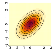
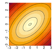
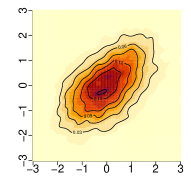
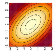
(b) Double Exponential distribution
Density	MD	LMD with $h=0.3$	LMD with $h=4$
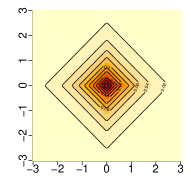
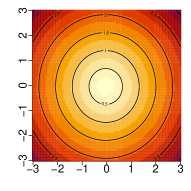
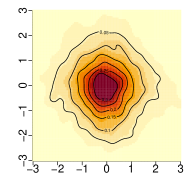
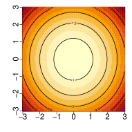
(c) Mixture Normal distribution
Density	MD	LMD with $h=0.4$	LMD with $h=5$

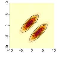
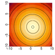
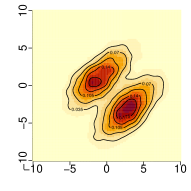
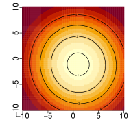
Figure 3: Contour plots of density, estimated MD, and estimated LMD with small and large values of $h$ in three examples involving elliptic (a) and non-elliptic (b and c) distributions.

Figure 4: Average misclassification rates of the LMD classifier for different values of $h$ in Example A (left) and Example B (right) involving elliptical and non-elliptical distributions, respectively.

A similar behavior can be observed for the classifier based on the local Mahalanobis distances. We formally define the classifier here. For a fixed $h>0$, we compute the empirical LMDs $\widehat{\Gamma}_{h}(\mathbf{x}_{ji})=\big{(}\widehat{\gamma}^{h}_{1}(\mathbf{x}_{ji}),\ldots,\widehat{\gamma}^{h}_{J}(\mathbf{x}_{ji})\big{)}$ for $j=1,\ldots,J$ and $i=1,\ldots,n_{j}$. These are used as feature vectors, and a GAM with logistic link is fitted on these features to model the posterior probabilities of different classes (cf. Theorem 3.1). Finally, an observation is classified to the class with the highest posterior probability estimated from the fitted GAM. We refer to the classifier as the LMD classifier. To demonstrate the performance of the LMD classifier for different values of $h$, we consider two examples involving binary classification. In Example A, the class distributions $N_{2}(-0.3{\bf 1}_{2},{\bf I}_{2})$ and $N_{2}(0.3{\bf 1}_{2},{\bf I}_{2})$ differ only in their locations. In Example B, both the classes are equal mixtures of two bivariate normal distributions. While one class is a mixture of $N_{2}\big{(}(1,-1)^{\top},\mbox{\boldmath$\Sigma$}\big{)}$ and $N_{2}\big{(}(-3,3)^{\top},\mbox{\boldmath$\Sigma$}\big{)}$, the other one is a mixture of $N_{2}\big{(}(-1,1)^{\top},\mbox{\boldmath$\Sigma$}\big{)}$ and $N_{2}\big{(}(3,-3)^{\top},\mbox{\boldmath$\Sigma$}\big{)}$, where $\mbox{\boldmath$\Sigma$}={\bf I}_{2}+4{\bf 1}_{2}{\bf 1}_{2}^{\top}$. For these two examples, we consider training and test samples of sizes 200 and 2000, respectively (equal number of observations from the two classes). The average misclassification rates of the LMD classifier for different choices of $h$ are shown in Figure 4. In Example A, where the distributions are elliptic, the LMD classifiers with large values of $h$ perform much better than those based on small values of $h$. But, in Example B, where the distributions are non-elliptic, we observe a diametrically opposite picture. Here, the LMD classifiers based on large values of $h$ do not perform well, but those based on smaller values of $h$ (e.g., $h=2.2$) have excellent performance. In this example, while the MD classifier misclassifies more than 30% observations, the LMD classifier with this choice of $h$ has a misclassification rate close to 18%.

These examples clearly show that the performance of the LMD classifier depends heavily on the value of $h$, and it needs to be chosen appropriately. In this article, we use the bootstrap method for this purpose. More specifically, we fix a collection of $h$ values, say $\{h_{1},\ldots,h_{k}\}$. For each of these $h$ values, we construct the LMD classifier, and compute the average misclassification rate of the classifier based on 100 bootstrap samples. Finally, the value of $h$ leading to the minimum average misclassification rate is selected for constructing the classifier. For selecting the collection $\{h_{1},\ldots,h_{k}\}$, we use the following strategy. We compute the pairwise Mahalanobis distances among the observations in a class, separately for all the classes. One-third of the fifth percentile of these pairwise distances is taken to be the lower limit $h_{1}$. Since LMD behaves like a shifted version of the squared MD for large values of $h$, for the upper limit, we choose a value of $h$ for which $\mathrm{LMD}$ is close to $K(\mathbf{0})(\mathrm{MD}^{2}+d)$ (cf. Lemma 3.1). In order to do this, we start with $h_{1}$ and keep increasing the value in a $\log$-scale taking $h_{i}=h_{1}k_{0}^{i-1}$ for $i\geq 2$ and some $k_{0}>1$ until the correlation between $\big{\{}\widehat{\gamma}_{j}^{h}(\mathbf{x}_{ji}):j=1,\ldots,J;~{}i=1,\ldots,n_{j}\big{\}}$ and $\big{\{}\big{(}\widehat{\delta}_{j}(\mathbf{x}_{ji})\big{)}^{2}+d:j=1,\ldots,J;i=1,\ldots,n_{j}\big{\}}$ becomes higher than a threshold $r$ close to $1$. We stop at the first instance when the correlation is higher than $r$ and all the intermediate $h$ values (including the one at which we stop, say $h_{k}$) constitute the set $\{h_{1},\ldots,h_{k}\}$. The performance of the LMD classifier in Examples 1–8 with the bootstrap selection of $h$ is shown in Table 3. We also show the results for the MD classifier for reference. It is clear from this table that the LMD classifier with bootstrapped choice of $h$ perform well and its misclassification rates are close to those of the MD classifier in Examples 1–8.

Classifier	$d$	Ex1	Ex 2	Ex 3	Ex 4	Ex 5	Ex 6	Ex 7	Ex 8
	2	6.85 $\scriptstyle(.27)$	35.14 $\scriptstyle(.15)$	31.80 $\scriptstyle(.09)$	4.72 $\scriptstyle(.24)$	37.82 $\scriptstyle(.13)$	51.65 $\scriptstyle(.13)$	46.52 $\scriptstyle(.11)$	35.01 $\scriptstyle(.09)$
MD	4	7.75 $\scriptstyle(.18)$	29.59 $\scriptstyle(.10)$	24.63 $\scriptstyle(.09)$	5.18 $\scriptstyle(.14)$	32.87 $\scriptstyle(.14)$	53.07 $\scriptstyle(.13)$	32.32 $\scriptstyle(.12)$	30.50 $\scriptstyle(.13)$
	6	8.46 $\scriptstyle(.18)$	26.00 $\scriptstyle(.11)$	20.09 $\scriptstyle(.11)$	4.80 $\scriptstyle(.15)$	30.95 $\scriptstyle(.17)$	53.83 $\scriptstyle(.13)$	26.82 $\scriptstyle(.12)$	28.30 $\scriptstyle(.29)$
	2	6.83 $\scriptstyle(.26)$	35.16 $\scriptstyle(.15)$	31.87 $\scriptstyle(.10)$	4.58 $\scriptstyle(.23)$	38.14 $\scriptstyle(.14)$	51.99 $\scriptstyle(.14)$	46.72 $\scriptstyle(.11)$	36.50 $\scriptstyle(.39)$
LMD	4	7.74 $\scriptstyle(.18)$	29.58 $\scriptstyle(.09)$	24.63 $\scriptstyle(.10)$	5.40 $\scriptstyle(.42)$	32.59 $\scriptstyle(.13)$	52.83 $\scriptstyle(.13)$	32.44 $\scriptstyle(.12)$	32.98 $\scriptstyle(.50)$
	6	8.42 $\scriptstyle(.18)$	25.96 $\scriptstyle(.11)$	19.89 $\scriptstyle(.11)$	4.55 $\scriptstyle(.12)$	30.57 $\scriptstyle(.17)$	53.24 $\scriptstyle(.14)$	27.29 $\scriptstyle(.26)$	32.46 $\scriptstyle(.72)$

Table 3: Average misclassification rates (in %) of MD and LMD (with bootstrap choice of $h$) classifiers in Examples 1–8. The corresponding standard errors are reported within brackets in a smaller font.

In order to take care of non-elliptic distributions and complex class boundaries, several classifiers based on kernelized Mahalanobis distance (KMD) have been proposed in the literature (see, e.g., Mika et al., 1999; Ruiz and López-de Teruel, 2001; Chatpatanasiri et al., 2010). But unlike LMD, KMD does not behave like the Mahalanobis distance for large values of $h$. Moreover, for small values of $h$, it converges to a constant, not to a constant multiple of the density function. So, the Bayes classifier cannot be expressed as a function of KMDs. Instead of LMD, when we used GAM based on KMD for classification, it led to poor results. For instance, in Example 1, while the MD and LMD classifiers had misclassification rates around 7–9%, the use of KMD yielded misclassification rates more than 25%. So, in this article, we do not consider it for further study.

3.1 Numerical examples involving non-elliptic distributions

Here, we consider some classification problems involving non-elliptic distributions for further evaluation of the performance of MD and LMD classifiers. Misclassification rates of some popular state-of-the-art classifiers (those considered in Section 2.1) are also reported for comparison. As in Section 2.1, we generate 100 observations from each class to form the training set, and 1000 observations from each class (5000 for two-class problems) to form the test set. For each example, we consider three different choices of $d$ (2, 4 and 6) as before, and each experiment is repeated 100 times. The average test set misclassification rates, and the corresponding standard errors, of different classifiers over these 100 repetititons are reported in Table 4.

Example 9.

We consider four multivariate Laplace distributions (the components are i.i.d. Laplace) with the same covariance matrix $0.75{\bf I}_{d}$ but different locations. The locations of these four classes are taken to be $\mathbf{1}_{d}$ , $-\mathbf{1}_{d}$, $\mathbf{a}_{d}$ and $-\mathbf{a}_{d}$, respectively, where the components of $\mathbf{a}_{d}$ are $(-1)^{i}$ for $i=1,\ldots,d$.

In this location problem, most of the classifiers barring the classification tree (CART) have satisfactory performance for all values of $d$. Among them, linear SVM has an edge for $d=2$ and LDA for $d=4$, but for $d=6$, the Random Forest classifier has the lowest misclassification rate. CART has higher misclassification rates for $d=4$ and $d=6$.

Example 10.

Here, we consider two multivariate exponential distributions with densities $f_{j}(\mathbf{x})=\lambda_{j}^{-d}e^{-\lambda_{j}^{-1}\sum_{i=1}^{d}x_{i}}\,{\mathbb{I}}_{\{x_{1},\ldots,x_{d}\geq 0\}}$ for $j=1,2$. We take the scale parameters $\lambda_{1}=1$ and $\lambda_{2}=2$.

In this scale problem, the Bayes classifier has a linear class boundary. So, as expected, linear classifiers perform better than their competitors. Among them, logistic regression has the lowest misclassification rate. Nonlinear SVM, MD and LMD classifiers have competitive performance. They perform better than other nonlinear classifiers like $k$NN, KDA, CART and Random Forest.

Data	$d$	Bayes	LDA	QDA	Logist	GLM	Neural	$k$NN	KDA	CART	Rand	SVM	SVM	MD	LMD
set					Reg.	Net	Net				Forest	Linear	Nonlin	Class	Class
	2	24.57	24.84	25.23	24.91	24.91	54.21	25.24	25.06	25.69	28.70	24.83	25.58	25.64	25.73
		$\scriptstyle(0.06)$	$\scriptstyle(0.07)$	$\scriptstyle(0.07)$	$\scriptstyle(0.07)$	$\scriptstyle(0.07)$	$\scriptstyle(1.02)$	$\scriptstyle(0.08)$	$\scriptstyle(0.07)$	$\scriptstyle(0.11)$	$\scriptstyle(0.12)$	$\scriptstyle(0.07)$	$\scriptstyle(0.08)$	$\scriptstyle(0.07)$	$\scriptstyle(0.07)$
Ex 9	4	15.58	15.96	16.52	16.27	16.31	50.75	16.22	16.08	20.59	17.53	16.29	16.66	17.17	17.20
		$\scriptstyle(0.05)$	$\scriptstyle(0.06)$	$\scriptstyle(0.06)$	$\scriptstyle(0.06)$	$\scriptstyle(0.06)$	$\scriptstyle(1.28)$	$\scriptstyle(0.07)$	$\scriptstyle(0.07)$	$\scriptstyle(0.19)$	$\scriptstyle(0.08)$	$\scriptstyle(0.05)$	$\scriptstyle(0.08)$	$\scriptstyle(0.07)$	$\scriptstyle(0.06)$
	6	7.74	10.19	11.07	10.80	10.73	51.70	10.30	10.01	19.20	9.46	10.85	10.47	11.98	12.04
		$\scriptstyle(0.04)$	$\scriptstyle(0.05)$	$\scriptstyle(0.06)$	$\scriptstyle(0.06)$	$\scriptstyle(0.06)$	$\scriptstyle(1.34)$	$\scriptstyle(0.05)$	$\scriptstyle(0.05)$	$\scriptstyle(0.18)$	$\scriptstyle(0.08)$	$\scriptstyle(0.06)$	$\scriptstyle(0.07)$	$\scriptstyle(0.07)$	$\scriptstyle(0.07)$
	2	31.96	32.28	33.56	32.18	32.44	33.70	33.71	34.75	35.47	37.85	32.51	33.90	33.18	33.23
		$\scriptstyle(0.05)$	$\scriptstyle(0.06)$	$\scriptstyle(0.06)$	$\scriptstyle(0.06)$	$\scriptstyle(0.10)$	$\scriptstyle(0.45)$	$\scriptstyle(0.19)$	$\scriptstyle(0.23)$	$\scriptstyle(0.25)$	$\scriptstyle(0.15)$	$\scriptstyle(0.08)$	$\scriptstyle(0.20)$	$\scriptstyle(0.13)$	$\scriptstyle(0.12)$
Ex 10	4	24.89	25.69	27.15	25.45	25.74	27.41	27.99	29.24	32.23	28.82	25.68	26.62	26.60	26.76
		$\scriptstyle(0.05)$	$\scriptstyle(0.06)$	$\scriptstyle(0.07)$	$\scriptstyle(0.06)$	$\scriptstyle(0.09)$	$\scriptstyle(0.64)$	$\scriptstyle(0.16)$	$\scriptstyle(0.21)$	$\scriptstyle(0.26)$	$\scriptstyle(0.13)$	$\scriptstyle(0.08)$	$\scriptstyle(0.10)$	$\scriptstyle(0.11)$	$\scriptstyle(0.11)$
	6	20.22	21.43	22.88	20.99	21.30	24.67	25.13	26.26	31.13	23.68	21.18	22.57	22.59	22.74
		$\scriptstyle(0.05)$	$\scriptstyle(0.07)$	$\scriptstyle(0.06)$	$\scriptstyle(0.07)$	$\scriptstyle(0.09)$	$\scriptstyle(0.91)$	$\scriptstyle(0.14)$	$\scriptstyle(0.20)$	$\scriptstyle(0.20)$	$\scriptstyle(0.10)$	$\scriptstyle(0.07)$	$\scriptstyle(0.14)$	$\scriptstyle(0.10)$	$\scriptstyle(0.11)$
	2	27.60	49.73	28.96	49.73	49.78	42.42	32.04	30.76	34.61	33.64	46.57	29.96	29.08	29.00
		$\scriptstyle(0.04)$	$\scriptstyle(0.10)$	$\scriptstyle(0.07)$	$\scriptstyle(0.10)$	$\scriptstyle(0.09)$	$\scriptstyle(0.42)$	$\scriptstyle(0.16)$	$\scriptstyle(0.14)$	$\scriptstyle(0.25)$	$\scriptstyle(0.13)$	$\scriptstyle(0.41)$	$\scriptstyle(0.22)$	$\scriptstyle(0.10)$	$\scriptstyle(0.09)$
Ex 11	4	15.26	49.27	17.37	49.28	49.35	41.18	23.87	22.64	31.74	21.77	45.47	17.61	17.52	17.50
		$\scriptstyle(0.03)$	$\scriptstyle(0.11)$	$\scriptstyle(0.06)$	$\scriptstyle(0.11)$	$\scriptstyle(0.11)$	$\scriptstyle(0.31)$	$\scriptstyle(0.12)$	$\scriptstyle(0.12)$	$\scriptstyle(0.28)$	$\scriptstyle(0.13)$	$\scriptstyle(0.40)$	$\scriptstyle(0.09)$	$\scriptstyle(0.07)$	$\scriptstyle(0.07)$
	6	8.76	48.85	11.30	48.87	48.99	39.91	21.06	19.79	30.73	15.86	44.30	11.54	11.66	11.62
		$\scriptstyle(0.03)$	$\scriptstyle(0.12)$	$\scriptstyle(0.05)$	$\scriptstyle(0.11)$	$\scriptstyle(0.11)$	$\scriptstyle(0.31)$	$\scriptstyle(0.13)$	$\scriptstyle(0.14)$	$\scriptstyle(0.23)$	$\scriptstyle(0.16)$	$\scriptstyle(0.39)$	$\scriptstyle(0.09)$	$\scriptstyle(0.08)$	$\scriptstyle(0.08)$
	2	0.00	49.83	43.43	49.83	49.59	43.98	10.69	10.02	24.86	12.71	50.55	7.38	21.42	14.92
		$\scriptstyle(0.00)$	$\scriptstyle(0.09)$	$\scriptstyle(0.43)$	$\scriptstyle(0.09)$	$\scriptstyle(0.13)$	$\scriptstyle(0.24)$	$\scriptstyle(0.17)$	$\scriptstyle(0.13)$	$\scriptstyle(0.29)$	$\scriptstyle(0.16)$	$\scriptstyle(0.14)$	$\scriptstyle(0.16)$	$\scriptstyle(0.14)$	$\scriptstyle(0.30)$
Ex 12	4	0.00	49.95	43.67	49.95	50.02	48.00	36.26	34.54	41.95	34.26	49.77	35.71	31.62	29.20
		$\scriptstyle(0.00)$	$\scriptstyle(0.06)$	$\scriptstyle(0.17)$	$\scriptstyle(0.06)$	$\scriptstyle(0.09)$	$\scriptstyle(0.14)$	$\scriptstyle(0.28)$	$\scriptstyle(0.22)$	$\scriptstyle(0.27)$	$\scriptstyle(0.16)$	$\scriptstyle(0.08)$	$\scriptstyle(0.22)$	$\scriptstyle(0.18)$	$\scriptstyle(0.18)$
	6	0.00	49.92	43.86	49.92	49.90	49.18	43.87	42.64	43.75	36.50	49.66	38.53	33.87	32.17
		$\scriptstyle(0.00)$	$\scriptstyle(0.05)$	$\scriptstyle(0.14)$	$\scriptstyle(0.05)$	$\scriptstyle(0.06)$	$\scriptstyle(0.13)$	$\scriptstyle(0.19)$	$\scriptstyle(0.24)$	$\scriptstyle(0.21)$	$\scriptstyle(0.16)$	$\scriptstyle(0.06)$	$\scriptstyle(0.23)$	$\scriptstyle(0.16)$	$\scriptstyle(0.18)$
	2	0.00	50.44	50.16	50.43	50.22	46.77	12.60	15.33	30.24	14.17	52.24	16.65	46.74	29.92
		$\scriptstyle(0.00)$	$\scriptstyle(0.27)$	$\scriptstyle(0.19)$	$\scriptstyle(0.27)$	$\scriptstyle(0.16)$	$\scriptstyle(0.19)$	$\scriptstyle(0.17)$	$\scriptstyle(0.19)$	$\scriptstyle(0.46)$	$\scriptstyle(0.20)$	$\scriptstyle(0.21)$	$\scriptstyle(0.23)$	$\scriptstyle(0.32)$	$\scriptstyle(0.29)$
Ex 13	4	0.00	50.12	50.14	50.12	50.00	48.45	29.08	28.96	45.61	36.55	51.25	30.27	48.93	34.04
		$\scriptstyle(0.00)$	$\scriptstyle(0.09)$	$\scriptstyle(0.10)$	$\scriptstyle(0.09)$	$\scriptstyle(0.05)$	$\scriptstyle(0.10)$	$\scriptstyle(0.24)$	$\scriptstyle(0.13)$	$\scriptstyle(0.28)$	$\scriptstyle(0.18)$	$\scriptstyle(0.11)$	$\scriptstyle(0.19)$	$\scriptstyle(0.14)$	$\scriptstyle(0.39)$
	6	0.00	50.32	50.06	50.30	50.12	48.91	37.17	38.74	48.07	42.39	50.84	35.90	49.39	36.42
		$\scriptstyle(0.00)$	$\scriptstyle(0.08)$	$\scriptstyle(0.10)$	$\scriptstyle(0.08)$	$\scriptstyle(0.05)$	$\scriptstyle(0.10)$	$\scriptstyle(0.33)$	$\scriptstyle(0.31)$	$\scriptstyle(0.23)$	$\scriptstyle(0.17)$	$\scriptstyle(0.10)$	$\scriptstyle(0.23)$	$\scriptstyle(0.12)$	$\scriptstyle(0.33)$
	2	0.00	49.99	50.80	49.99	49.92	40.20	0.00	0.00	1.83	1.79	59.49	0.00	44.22	0.00
		$\scriptstyle(0.00)$	$\scriptstyle(0.04)$	$\scriptstyle(0.88)$	$\scriptstyle(0.04)$	$\scriptstyle(0.20)$	$\scriptstyle(0.54)$	$\scriptstyle(0.00)$	$\scriptstyle(0.00)$	$\scriptstyle(0.07)$	$\scriptstyle(0.04)$	$\scriptstyle(0.39)$	$\scriptstyle(0.00)$	$\scriptstyle(0.69)$	$\scriptstyle(0.00)$
Ex 14	4	0.00	50.02	50.53	50.02	50.00	38.74	0.26	0.18	1.78	0.50	57.65	0.15	47.69	0.00
		$\scriptstyle(0.00)$	$\scriptstyle(0.04)$	$\scriptstyle(0.34)$	$\scriptstyle(0.04)$	$\scriptstyle(0.16)$	$\scriptstyle(0.31)$	$\scriptstyle(0.13)$	$\scriptstyle(0.07)$	$\scriptstyle(0.05)$	$\scriptstyle(0.03)$	$\scriptstyle(0.38)$	$\scriptstyle(0.10)$	$\scriptstyle(0.38)$	$\scriptstyle(0.00)$
	6	0.00	50.03	50.17	50.03	49.89	41.05	10.95	17.49	1.85	0.14	55.73	15.85	49.40	5.96
		$\scriptstyle(0.00)$	$\scriptstyle(0.03)$	$\scriptstyle(0.15)$	$\scriptstyle(0.03)$	$\scriptstyle(0.26)$	$\scriptstyle(0.44)$	$\scriptstyle(0.42)$	$\scriptstyle(0.24)$	$\scriptstyle(0.07)$	$\scriptstyle(0.01)$	$\scriptstyle(0.39)$	$\scriptstyle(0.38)$	$\scriptstyle(0.15)$	$\scriptstyle(0.22)$

Boldface character signifies the best result in each case.

Table 4: Average misclassification rates (in %) of different classifiers in Examples 9–14 for varying $d$. The corresponding standard errors are reported in the next line within brackets in a smaller font.

Example 11.

In this example, we consider two mixture normal distributions. The distribution corresponding to the first class is an equal mixture of $N_{d}(\mathbf{1}_{d},{\bf I}_{d})$ and $N(-\mathbf{1}_{d},{\bf I}_{d})$, whereas that for the second class is an equal mixture of $N_{d}(\mathbf{a}_{d},4{\bf I}_{d})$ and $N_{d}(-\mathbf{a}_{d},4{\bf I}_{d})$. Here, $\mathbf{a}_{d}$ is as defined in Example 9.

Here, the Bayes class boundary is nonlinear. So, the nonlinear classifiers outperform the linear classifiers. Overall performances of QDA, nonlinear SVM, MD and LMD classifiers are much better than the other classifiers considered here.

Example 12.

For this example, we generate observations from the uniform distribution on the hypercube $[-2,2]^{d}$. An observation $\mathbf{x}=(x_{1},\ldots,x_{d})^{\top}$ is assigned to Class-$1$ if $1/2<\prod_{i=1}^{d}|x_{i}|<2$. Otherwise, it is assigned to Class-$2$.

In this example, the LMD classifier performs much better than the MD classifier, especially for $d=2$. For $d=4$ and $d=6$, while most of the other classifiers perform poorly and have misclassification rates in excess of 40%, these two classifiers have misclassification rates close to 30%. They have the two best overall performances followed by Random Forest and nonlinear SVM.

Example 13.

The two underlying populations are mixtures of three uniform distributions. Let $R_{(a,b)}(\mathbf{z})$ be the region $\{\mathbf{x}\in\mathbb{R}^{d}:a\leq\|\mathbf{x}-\mathbf{z}\|\leq b\}$. Class-1 is a mixture of uniform distribuions on $R_{(0,1)}(-\mathbf{c})$, $R_{(1,2)}(\mathbf{c})$ and $R_{(2,3)}(-\mathbf{c})$ with mixing proportions $0.25$, $0.5$ and $0.25$, respectively, where $\mathbf{c}=(5,0,\ldots,0)^{\top}$. Class-2 is obtained if $\mathbf{c}$ is replaced by $-\mathbf{c}$ in the description of Class-1.

Here also, the LMD classifier outperforms the MD classifier. For $d=2$, $k$NN has the lowest misclassification rate followed by the Random Forest and the nonlinear SVM classifier. The LMD classifier has the fourth best misclassification rate. The performance of most of the classifiers, including $k$NN and Random Forest, deteriorates as the dimension increases. For $d=6$, while the nonlinear SVM and the LMD classifier have misclassification rates close to 35%, all other classifiers barring $k$NN and KDA misclassify more than 40% observations.

Example 14.

For Class-1, all the components are i.i.d., and their distributions are equal mixtures of $N(1,0.01)$ and $N(-1,0.01)$. The distribution for Class-2 is a rotated version of the distribution for Class-1, where we rotate each successive pair of covariates using the $45^{\circ}$ rotation matrix

$$\begin{pmatrix}1/\sqrt{2}&-1/\sqrt{2}\\ 1/\sqrt{2}&1/\sqrt{2}\end{pmatrix}.$$

Here, the LMD classifier has significantly better performance than the MD classifier, irrespective of the dimension. Besides LMD, the overall performances of CART and Random Forest are also good. The performances of $k$NN and KDA are exceptionally good for $d=2$. However, their performance deteriorates as the dimension increases. The rest of the classifiers have very poor performance.

4 High Dimension, Low Sample Size Behaviour of MD and LMD Classifiers

In this section, we consider the high dimension, low sample size (HDLSS) scenario, where the dimension of the data is much larger compared to the sample size. This type of data is frequently encountered in microarray gene expression studies, medical image analyses, spectral measurements in chemometrics, etc. The characteristic property of this type of data is the scarcity of observations compared to the number of variables, which makes the existing methods unsuitable. For instance, popular parametric classifiers like LDA and QDA cannot be used in HDLSS situations due to the singularity of the sample covariance matrices. On the other hand, nonparametric classifiers like KDA and $k$NN often lead to poor performance in HDLSS situations, especially when the competing classes vary widely in their scales (see, e.g., Hall et al., 2005). The proposed MD and LMD classifiers in their present form are also not usable in HDLSS situations because they involve the inverse of the sample covariance matrices. Here, we first modify the proposed MD and LMD classifiers so that they can be used in HDLSS situations. Next, we study the behavior of the modified classifiers under the HDLSS setup, both theoretically and empirically.

Note that if the dimension of the data exceeds the sample size, we cannot use the sample covariance matrices for computing the empirical versions of the Mahalanobis distances or their localized versions since they are not invertible. Hence, for such data, we propose to modify the MD (respectively, LMD) classifier by using the identity matrix or the diagonal of the sample covariance matrices in the computation of the Mahalanobis distances (respectively, localized Mahalanobis distances). After computing the distances, the classifier is constructed as before by fitting a GAM with logistic link. Also, we use the bootstrap method to select the localization parameter $h$ for the LMD classifier. These modified classifiers have excellent empirical performance in Example 1 with $d=500$. All of them correctly classify almost all observations, whereas many popular classifiers fail to achieve satisfactory performance (see Example 19 in Table 5). Motivated by this, we now investigate the theoretical behaviour of these modified classifiers under the HDLSS asymptotic regime, where the sample sizes $n_{1},\ldots,n_{J}$ (with $\min\{n_{1},\ldots,n_{J}\}\geq 2)$ remain fixed and the dimension $d$ diverges to infinity. For our investigation, we make some assumptions which are given below. In the following, $\mathbf{X}=(X_{1},\ldots,X_{d})^{\top}$, $\mathbf{Y}=(Y_{1},\ldots,Y_{d})^{\top}$ and $\mathbf{Z}=(Z_{1},\ldots,Z_{d})^{\top}$ are generic random vectors. Also, we denote the mean and the covariance of Class-$j$ by $\mbox{\boldmath$\mu$}_{j}$ and $\mbox{\boldmath$\Sigma$}_{j}$, respectively, for $j=1,\ldots,J$.

1. For all $1\leq j,j^{\prime}\leq J$, and three independent random vectors $\mathbf{X}$ from Class-$j$ and $\mathbf{Y},\vec{Z}$ from Class-$j^{\prime}$, we have $\Big{|}d^{-1}\sum_{i=1}^{d}(X_{i}-Y_{i})(X_{i}-Z_{i})-\mathbb{E}\big{\{}d^{-1}\sum_{i=1}^{d}(X_{i}-Y_{i})(X_{i}-Z_{i})\big{\}}\Big{|}\stackrel{{\scriptstyle\mathbb{P}}}{{\rightarrow}}0$ and $\Big{|}d^{-1}\sum_{i=1}^{d}(X_{i}-Y_{i})^{2}-\mathbb{E}\big{\{}d^{-1}\sum_{i=1}^{d}(X_{i}-Y_{i})^{2}\big{\}}\Big{|}\stackrel{{\scriptstyle\mathbb{P}}}{{\rightarrow}}0$ as $d\rightarrow\infty$.

2. For all $j=1,\ldots,J$, there exists a constant $\sigma_{j}^{2}$ such that $d^{-1}\mathrm{trace}(\mbox{\boldmath$\Sigma$}_{j})\to\sigma_{j}^{2}$ as $d\to\infty$. Also, for every $1\leq j\neq j^{\prime}\leq J$, there exists a constant $\nu_{jj^{\prime}}^{2}$ such that $d^{-1}\|\mbox{\boldmath$\mu$}_{j}-\mbox{\boldmath$\mu$}_{j^{\prime}}\|^{2}\to\nu_{jj^{\prime}}^{2}$ as $d\to\infty$.

These assumptions are pretty standard in the context of HDLSS asymptotics. Hall et al. (2005) considered the $d$-dimensional observations as time series truncated at time $d$ and studied the behaviour of pairwise distances as $d$ increases. They proved some distance convergence results under uniform boundedness of the fourth moments and $\rho$-mixing property of the time series. Assumption (A1) holds under those conditions. One can also assume some sufficient moment conditions like $\mathbb{V}\mathrm{ar}(\|\mathbf{X}-\mbox{\boldmath$\mu$}_{j}\|^{2})=o(d^{2})$, $\mathbb{V}\mathrm{ar}(\|\mathbf{Y}-\mbox{\boldmath$\mu$}_{j}\|^{2})=o(d^{2})$, $\mathrm{trace}(\mbox{\boldmath$\Sigma$}^{2}_{i})=o(d^{2})$ and $\mathrm{trace}(\mbox{\boldmath$\Sigma$}^{2}_{j})=o(d^{2})$ for (A1) to hold (Banerjee and Ghosh, 2023). Some other relevant conditions can be found in Ahn et al. (2007); Jung and Marron (2009); Aoshima and Yata (2018); Sarkar and Ghosh (2019); Yata and Aoshima (2020). Under (A1) and (A2), we have high dimensional convergence of estimated Mahalanobis distances, as shown below. The following result is stated for the case when the identity matrix is used for all the classes in the computation of the Mahalanobis distances. The case of diagonal covariance matrices is analogous, where we need to assume (A1) and (A2) for the standardized variables.

Theorem 4.1.

Let $\mathbf{X}_{j1},\ldots,\mathbf{X}_{jn_{j}}\stackrel{{\scriptstyle iid}}{{\sim}}F_{j}$ for $j=1,\ldots,J$ be independent collections of observations, and the distributions $F_{1},\ldots,F_{J}$ satisfy (A1) and (A2). Suppose that $\widehat{}\mbox{\boldmath$\mu$}_{j}=\overline{\mathbf{X}}_{j}=n_{j}^{-1}\sum_{i=1}^{n_{j}}\mathbf{X}_{ji}$ and $\widehat{}\mbox{\boldmath$\Sigma$}_{j}=\mathbf{I}$ are used as estimators of $\mbox{\boldmath$\mu$}_{j}$ and $\mbox{\boldmath$\Sigma$}_{j}$, respectively, for $j=1,\ldots,J$. Then, we have the following as $d\to\infty$.

1. For any $j=1,\ldots,J$ and $i=1,\ldots,n_{j}$, $d^{-1}\,\widehat{\Delta}(\mathbf{X}_{ji})\stackrel{{\scriptstyle\mathbb{P}}}{{\rightarrow}}\Theta_{j}=(\theta_{j1},\ldots,\theta_{jJ})$, where

   $$\theta_{jk}=\begin{cases}\Big{(}1-\frac{1}{n_{j}}\Big{)}\sigma_{j}^{2}&\text{if }k=j,\\ \nu_{jk}^{2}+\sigma_{j}^{2}+\frac{\sigma_{k}^{2}}{n_{k}}&\text{if }k\neq j.\end{cases}$$

2. For an independent observation $\mathbf{Z}\sim F_{i}$, $d^{-1}\,\widehat{\Delta}(\mathbf{Z})\stackrel{{\scriptstyle\mathbb{P}}}{{\rightarrow}}\Theta_{i}^{\ast}=(\theta^{\ast}_{i1},\ldots,\theta^{\ast}_{iJ})$, where

   $$\theta^{\ast}_{ik}=\begin{cases}\Big{(}1+\frac{1}{n_{i}}\Big{)}\sigma_{i}^{2}&\text{if }k=i,\\ \nu_{ik}^{2}+\sigma_{i}^{2}+\frac{\sigma_{k}^{2}}{n_{k}}&\text{if }k\neq i.\end{cases}$$

Part (a) of the above theorem shows that under (A1) and (A2), for the training sample observations from Class-$j$, the feature vectors $\widehat{\Delta}(\mathbf{X}_{ji})$ containing Mahalanobis distances tend to cluster around $\Theta_{j}$ when the dimension is large. Note that for $j\neq j^{\prime}$, $\Theta_{j}=\Theta_{j^{\prime}}$ implies $\sigma_{j}^{2}=\sigma_{j^{\prime}}^{2}$ and $\nu^{2}_{jj^{\prime}}=0$. So, if the distributions differ either in their locations or in their scales (i.e., for all $j\neq j^{\prime}$, either $\nu^{2}_{jj^{\prime}}>0$ or $\sigma_{j}^{2}\neq\sigma_{j^{\prime}}^{2}$), then ${\widehat{\Delta}}(\mathbf{X}_{ji})$’s converge to $J$ distinct points (one corresponding to each of the competing classes) on the feature space. Naturally, the classifier based on GAM classifies these $J$ points correctly. It partitions the observation space in such a way that these $J$ points belong to $J$ different regions formed by the partition. As a result, the training sample error becomes close to $0$ when $d$ is large. From part (b) of Theorem 4.1, it is also clear that if the sample sizes are not too small, then for a test observation $\mathbf{Z}$ from Class-$i$, $\widehat{\Delta}(\mathbf{Z})$ lies very close to $\Theta_{i}$. As a result, it is also correctly classified by the MD classifier with high probability. So, the test set misclassification rate of the MD classifier is also often close to $0$ for large $d$. This is demonstrated in Figure 5 for an experiment with observations from two competing normal populations $N_{d}(\mathbf{0}_{d},\mathbf{I}_{d})$ and $N_{d}(\mathbf{0}_{d},1.5\mathbf{I}_{d})$ differing only in their scales, where dimension of the data is $d=500$ and the training (respectively, test) dataset is taken to be of size 200 (respectively, 2000), such that an equal number of observations come from each class. From Figure 5, we can see that the estimated Mahalanobis distances in the training set and the test set are closely clustered. Moreover, the decision boundary from the fitted GAM perfectly separates the test data points. We have seen a similar phenomena in most of our numerical examples.

A result similar to Theorem 4.1 can be derived for LMD as well. The following theorem shows the high dimensional behavior of LMD under (A1) and (A2) when the tuning parameter $h$ increases with the dimension at an appropriate rate.

Theorem 4.2.

Let $\mathbf{X}_{j1},\ldots,\mathbf{X}_{jn_{j}}\stackrel{{\scriptstyle iid}}{{\sim}}F_{j}$ for $j=1,\ldots,J$ be independent collections of observations, and the distributions $F_{1},\ldots,F_{J}$ satisfy (A1) and (A2). Suppose that $\widehat{}\mbox{\boldmath$\Sigma$}_{j}=\mathbf{I}$ is used in the computation of empirical LMD for $j=1,\ldots,J$. Also, suppose that $\Psi$ is continuous and $h$ increases with $d$ in such a way that $h^{2}/d\rightarrow C_{0}>0$ as $d\rightarrow\infty$. For $1\leq j,j^{\prime}\leq J$, define $\theta_{jj^{\prime}}^{\circ}=\Psi\Big{(}\frac{\sigma_{j}^{2}+\sigma_{j^{\prime}}^{2}+\nu_{jj^{\prime}}^{2}}{C_{0}}\Big{)}(\sigma_{j}^{2}+\sigma_{j^{\prime}}^{2}+\nu_{jj^{\prime}}^{2})$, where $\nu^{2}_{jj}=0$. Then, we have the following as $d\to\infty$.

1. For any $j=1,\ldots,J$ and $i=1,\ldots,n_{j}$, $d^{-1}\,\widehat{\Gamma}_{h}(\mathbf{X}_{ji})\stackrel{{\scriptstyle\mathbb{P}}}{{\rightarrow}}\widetilde{\Theta}_{j}=(\widetilde{\theta}_{j1},\ldots,\widetilde{\theta}_{jJ})$, where

   $$\widetilde{\theta}_{jk}=\begin{cases}\Big{(}1-\frac{1}{n_{j}}\Big{)}\theta_{jj}^{0}&\text{if }k=j,\\ \theta_{jk}^{0}&\text{if }j\neq k.\end{cases}$$

2. For an independent observation $\mathbf{Z}\sim F_{i}$, $d^{-1}\,\widehat{\Gamma}_{h}(\mathbf{Z})\stackrel{{\scriptstyle\mathbb{P}}}{{\rightarrow}}\Theta_{i}^{\circ}=(\theta^{\circ}_{i1},\ldots,\theta^{\circ}_{iJ})$.

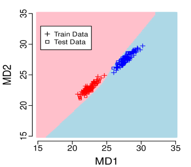
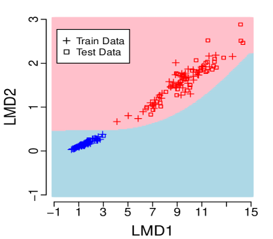
Figure 5: Decision boundary estimated by MD and LMD classifier (with bootstrap choice of h) along with scatter plots of empirical MD and LMD in a high-dimensional scale problem.

From the proof of the theorem, it can be seen that the result continues to hold for a data driven choice of the localization parameter $h$, as long as $h^{2}/d\overset{\mathbb{P}}{\to}C_{0}$ as $d\to\infty$. From part (a) of Theorem 4.1, it follows that if $h$ is chosen based on the median heuristic, it satisfies this condition. The condition is also satisfied if $h$ is chosen based on quantiles of pairwise distances. If the choice of the function $\Psi$ ensures that $\widetilde{\Theta}_{1},\ldots,\widetilde{\Theta}_{J}$ are distinct, then the feature vectors of estimated LMDs obtained from the training data converge to $J$ distinct points, one for each class. As a result, the classifier based on GAM correctly classifies these $J$ points. If the training sample sizes are not too small, the limiting behaviour of the feature vectors for all the test sample observations is the same as that of the training sample from the corresponding classes. Hence, similar to the MD classifier, the test cases are also correctly classified by the LMD classifier, and its error rate becomes close to $0$. This behavior of the LMD classifier can be seen in Figure 5, where we show the decision boundary of the LMD classifier and the scatter plots of the estimated LMDs for the training and the test samples.

Note that for the Gaussian kernel, the function $x\Psi(x/C_{0})$ is monotonically increasing for $x<C_{0}$ and monotonically decreasing for $x>C_{0}$. So, in a two-class problem, if $d_{11}:=2\sigma_{1}^{2}$, $d_{12}:=\sigma_{1}^{2}+\sigma_{2}^{2}+\nu_{12}^{2}$ and $d_{22}:=2\sigma_{2}^{2}$ are on the same side of $C_{0}$, we have $\Theta_{1}^{\circ}=\Theta_{2}^{\circ}$ only when $d_{11}=d_{12}=d_{22}$, which in turn implies $\sigma_{1}^{2}=\sigma_{2}^{2}$ and $\nu_{12}^{2}=0$. One can always choose the tuning parameter $h$ (which determines $C_{0}$) in such a way that $d_{11},d_{12}$ and $d_{22}$ belong to either $(-\infty,C_{0}]$ or $[C_{0},\infty)$. For instance, we can use the median heuristic on the observations from the two classes separately and use the smaller of the two as the tuning parameter. In that case, $\min\{d_{11},d_{22}\}/d$ plays the role of $C_{0}$ (note that $d_{12}$ cannot be smaller than both $d_{11}$ and $d_{22}$). A similar strategy works for classification problems involving more than two classes and also when the localization parameter is chosen based on the quantiles of the pairwise distances. However, this requirement is not necessary for $\Theta_{j}^{\circ}\neq\Theta_{j^{\prime}}^{\circ}$ to hold.

4.1 Simulation Results

To investigate the empirical behaviour of our proposed MD and LMD classifiers for high-dimensional data, here we consider some high-dimensional simulated examples. We take $d=500$, and in each case, the training set (respectively, the test set) is formed by taking 100 (respectively, 1000) observations from each class. Each experiment is repeated 100 times to compute the average test set misclassification errors of different classifiers and their corresponding standard errors. These are reported in Table 5. For MD and LMD classifiers, we use both the identity matrix and the diagonal of the sample covariance matrix, and report the best result out of these two choices (separtely for MD and LMD). The same strategy is adopted for LDA as well. For QDA, we use the diagonal of the sample covariance matrix.

Example 15.

We consider a location problem involving normal distributions $N_{500}(-0.2{\bf 1}_{500},\mbox{\boldmath$\Sigma$}_{500})$ and $N_{500}(0.2{\bf 1}_{500},\mbox{\boldmath$\Sigma$}_{500})$. Here, $\mbox{\boldmath$\Sigma$}_{500}=((\rho^{|i-j|}))$ is an auto-correlation matrix with $\rho=0.75$.

As expected, in this location problem, LDA has the best performance, but the error rates of the other two linear classifiers, GLMNET and linear SVM, are slightly higher. CART has poor performance in this high-dimensional example. Performances of all other classifiers are fairly satisfactory.

Example	Bayes	LDA	QDA	GLM	Neural	$k$NN	KDA	CART	Rand	SVM	SVM	MD	LMD
set				NET	NET				Forest	Linear	Nonlin	Class	Class
Ex. 15	4.51	5.13	5.38	12.86	9.40	6.41	6.13	38.93	6.78	7.94	5.48	5.90	5.87
	$\scriptstyle(0.08)$	$\scriptstyle(0.09)$	$\scriptstyle(0.09)$	$\scriptstyle(0.16)$	$\scriptstyle(0.15)$	$\scriptstyle(0.10)$	$\scriptstyle(0.14)$	$\scriptstyle(0.22)$	$\scriptstyle(0.10)$	$\scriptstyle(0.12)$	$\scriptstyle(0.09)$	$\scriptstyle(0.10)$	$\scriptstyle(0.10)$
Ex. 16	0.00	48.48	0.91	49.28	49.81	50.00	50.00	44.83	12.98	49.11	1.74	0.91	0.45
	$\scriptstyle(0.00)$	$\scriptstyle(0.16)$	$\scriptstyle(0.03)$	$\scriptstyle(0.16)$	$\scriptstyle(0.15)$	$\scriptstyle(0.00)$	$\scriptstyle(0.00)$	$\scriptstyle(0.25)$	$\scriptstyle(0.16)$	$\scriptstyle(0.15)$	$\scriptstyle(0.06)$	$\scriptstyle(0.14)$	$\scriptstyle(0.04)$
Ex. 17	0.00	49.70	50.00	49.94	49.92	49.90	49.99	48.26	33.41	50.08	19.61	13.50	5.17
	$\scriptstyle(0.00)$	$\scriptstyle(0.16)$	$\scriptstyle(0.00)$	$\scriptstyle(0.17)$	$\scriptstyle(0.15)$	$\scriptstyle(0.02)$	$\scriptstyle(0.01)$	$\scriptstyle(0.18)$	$\scriptstyle(0.17)$	$\scriptstyle(0.15)$	$\scriptstyle(0.18)$	$\scriptstyle(0.55)$	$\scriptstyle(0.11)$
Ex. 18	0.00	48.70	49.33	43.87	42.54	50.17	25.19	43.76	22.54	42.34	28.69	37.86	0.16
	$\scriptstyle(0.00)$	$\scriptstyle(0.40)$	$\scriptstyle(0.37)$	$\scriptstyle(0.23)$	$\scriptstyle(0.16)$	$\scriptstyle(0.15)$	$\scriptstyle(0.12)$	$\scriptstyle(0.29)$	$\scriptstyle(0.40)$	$\scriptstyle(0.15)$	$\scriptstyle(0.53)$	$\scriptstyle(1.50)$	$\scriptstyle(0.03)$
Ex. 19	0.00	50.01	48.25	50.23	40.32	0.00	0.00	1.72	0.00	50.16	0.00	3.80	0.00
	$\scriptstyle(0.00)$	$\scriptstyle(0.11)$	$\scriptstyle(0.78)$	$\scriptstyle(0.23)$	$\scriptstyle(0.25)$	$\scriptstyle(0.00)$	$\scriptstyle(0.00)$	$\scriptstyle(0.05)$	$\scriptstyle(0.00)$	$\scriptstyle(0.11)$	$\scriptstyle(0.00)$	$\scriptstyle(0.73)$	$\scriptstyle(0.00)$
Ex. 20	0.00	44.86	50.00	46.02	45.49	50.00	50.00	40.94	34.46	44.78	41.67	0.00	0.14
	$\scriptstyle(0.00)$	$\scriptstyle(0.13)$	$\scriptstyle(0.00)$	$\scriptstyle(0.17)$	$\scriptstyle(0.16)$	$\scriptstyle(0.00)$	$\scriptstyle(0.00)$	$\scriptstyle(0.27)$	$\scriptstyle(0.38)$	$\scriptstyle(0.14)$	$\scriptstyle(0.49)$	$\scriptstyle(0.00)$	$\scriptstyle(0.08)$
Ex. 21	4.28	48.64	22.15	47.34	49.13	50.00	14.26	40.69	17.37	45.85	15.82	17.42	6.84
	$\scriptstyle(0.0)$	$\scriptstyle(0.23)$	$\scriptstyle(1.36)$	$\scriptstyle(0.18)$	$\scriptstyle(0.17)$	$\scriptstyle(0.00)$	$\scriptstyle(0.15)$	$\scriptstyle(0.28)$	$\scriptstyle(0.12)$	$\scriptstyle(0.11)$	$\scriptstyle(0.13)$	$\scriptstyle(0.67)$	$\scriptstyle(0.49)$
Ex. 22	0.00	50.08	50.00	49.52	48.15	49.94	50.02	50.04	50.01	48.70	49.31	48.94	1.13
	$\scriptstyle(0.00)$	$\scriptstyle(0.15)$	$\scriptstyle(0.00)$	$\scriptstyle(0.16)$	$\scriptstyle(0.18)$	$\scriptstyle(0.03)$	$\scriptstyle(0.03)$	$\scriptstyle(0.13)$	$\scriptstyle(0.17)$	$\scriptstyle(0.15)$	$\scriptstyle(0.17)$	$\scriptstyle(0.42)$	$\scriptstyle(0.68)$

Boldface character signifies the best result in each case.

Table 5: Average misclassification rates (in %) of different classifiers in Examples 15–22. The standard errors are reported in the next line within brackets in a smaller font.

Example 16.

This is a scale problem with two multivariate normal distributions $N_{500}({\bf 0}_{500},\mbox{\boldmath$\Sigma$}_{500})$ and $N_{500}({\bf 0}_{500},2\mbox{\boldmath$\Sigma$}_{500})$, where $\mbox{\boldmath$\Sigma$}_{500}$ is the same as in Example 15.

In this problem, as expected QDA performs well, whereas all linear classifiers have misclassification rates close to 50%. KDA and $k$NN also have poor performance. The reason behind the failure of $k$NN can be explained following Hall et al. (2005). A similar argument can be given for KDA as well. CART also performs poorly, but the Random Forest has relatively better performance. Apart from QDA, nonlinear SVM, MD and LMD classifiers have excellent performance. Among them, the LMD classifier has an edge.

The next three examples deal with binary classification involving mixture normal distributions.

Example 17.

Class-$1$ is an equal mixture of $N_{500}(0.05{\bf 1}_{500},0.20{\bf I}_{500})$ and $N_{500}(-0.05{\bf 1}_{500},0.20{\bf I}_{500})$, while Class-$2$ is an equal mixture of $N_{500}(0.05{\bf a}_{500},0.25{\bf I}_{500})$ and $N_{500}(-0.05{\bf a}_{500},0.25{\bf I}_{500})$, where $\mathbf{a}_{500}=(-1,1,-1,1,\ldots,-1,1)^{\top}$ is as defined in Example 9.

Example 18.

Class-$1$ is an equal mixture of $N_{500}(0.5{\bf 1}_{500},{\bf I}_{500})$ and $N_{500}(-0.5{\bf 1}_{500},4{\bf I}_{500})$. Class-$2$ is an equal mixture of $N_{500}(0.5{\bf a}_{500},{\bf I}_{500})$ and $N_{500}(-0.5{\bf a}_{500},4{\bf I}_{500})$.

In these two examples, the LMD classifier outperforms all its competitors. The MD classifier also has reasonably good performance in Example 17, but in Example 18, its misclassification rate is much higher. In these two examples, the competing classes do not satisfy assumptions (A1) and (A2), but each of the sub-classes satisfies these properties. So, depending on which of the two sub-classes an observation is coming from, the scaled version of $\widehat{\Delta}(\cdot)$ converges to two different points. It is not difficult to check that in the case of Example 18, these two points for one class are nearly the same as the corresponding points from the competing class (see the left panel of Figure 6). This indistinguishability is the reason behind the poor performance of the MD classifier. For the LMD classifier, however, these four points (two from each class) are well separated (see the right panel of Figure 6). As a result, the LMD classifier correctly classifies almost all observations.

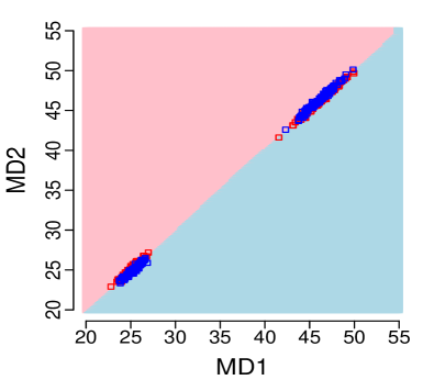
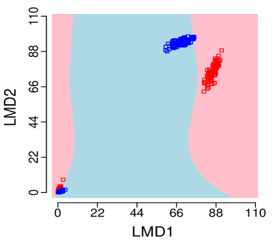
Figure 6: Decision boundary of MD and LMD (with bootstrap choice of $h$) classifiers along with scatter plots of empirical MD and LMD in Example 18.

Example 19.

Both classes are equal mixtures of four normal distributions, each with covariance matrix $0.01\mathbf{I}_{d}$. For Class-$1$, the locations of the four sub-populations are $\mathbf{a}_{d}$, $-\mathbf{a}_{d}$, $\mathbf{1}_{d}$ and $-\mathbf{1}_{d}$. For Class-$2$, we take a rotation of the distribution for Class-$1$, where we rotate each successive pair of covariates by $45^{\circ}$ as done in Example 14.

Here, the LMD classifier has zero misclassification rate along with $k$NN, KDA, Random Forest and Nonlinear SVM. CART and MD also have misclassification rates less than $5\%$. The rest of the classifiers have more than $40\%$ misclassification rates.

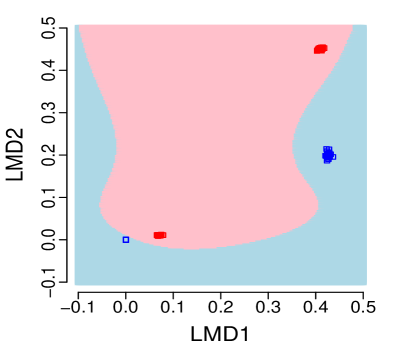
Figure 7: Decision boundary of MD and LMD (with bootstrap choice of $h$) classifiers along with scatter plots of empirical MD and LMD in Example 20.

Example 20.

Class-1 is an equal mixture of $U_{500}(0,1)$ and $U_{500}(2,3)$, while Class-2 is an equal mixture of $U_{500}(1,2)$ and $U_{500}(3,4)$. Here, $U_{d}(a,b)$ is the uniform distribution on $\{\mathbf{x}\in\mathbb{R}^{500}:a\leq\|\mathbf{x}\|\leq b\}$, as defined in Example 1.

This is a high-dimensional version of Example 1. Here, one can show that the sub-classes satisfy (A1) and (A2) following Sarkar and Ghosh (2019). This is also quite evident from Figure 7, where we plot the decision boundaries of the MD and LMD classifiers along with the scatter plots of the MD and LMD values for the two classes. In this example, both MD and LMD classifiers have excellent performance. Their misclassification rates are very close to zero, while all the other classifiers have much higher misclassification rates.

Example 21.

We consider a classification problem between $N_{500}({\bf 0}_{500},3{\bf I}_{500})$ and the $500$-dimensional standard $t$ distribution with $3$ degrees of freedom.

This is the high-dimensional version of Example 5, where the underlying distributions have the same mean and covariance, but differ in their shapes. Here, the assumption (A1) does not hold, and we analyze this dataset to investigate the performance of the MD and LMD classifiers under departure from the stipulated assumptions. Table 5 shows that even in this example, the LMD classifier outperforms its competitors. Among the rest, KDA, nonlinear SVM, Random Forest, and the MD classifier have relatively better performance.

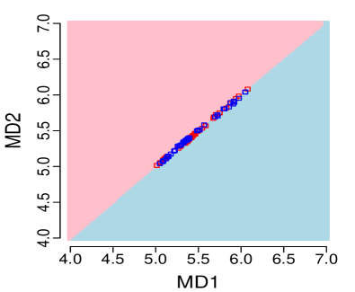
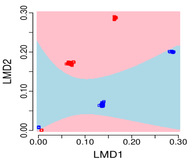
Figure 8: Decision boundary of MD and LMD (with bootstrap choice of $h$) classifiers along with scatter plots of empirical MD and LMD in Example 22.

Example 22.

Class-1 is a mixture of uniform distributions on $R_{(0,1)}(-\mathbf{c})$, $R_{(1,2)}(\mathbf{c})$ and $R_{(2,3)}(-\mathbf{c})$ with mixing proportions $0.25$, $0.5$ and $0.25$, respectively. Class-2 is a mixture of uniform distributions on $R_{(0,1)}(\mathbf{c})$, $R_{(1,2)}(-\mathbf{c})$ and $R_{(2,3)}(\mathbf{c})$ with mixing proportions $0.25$, $0.5$ and $0.25$, respectively. Here, $R_{(a,b)}(\mathbf{z})=\{\mathbf{x}\in\mathbb{R}^{500}:a\leq\|\mathbf{x}-\mathbf{z}\|\leq b\}$ and $\mathbf{c}=(5,0,\ldots,0)^{\top}$ are as defined in Example 13.

This example is the high-dimensional version of Example 13. Here, the LMD classifier has excellent performance, while all other classifiers including the MD classifier misclassify almost half of the observations. The reason behind this diametrically opposite behaviour of MD and LMD classifiers is the same as that in Example 18; indistinguishability (respectively, distinguishability) of the two populations in terms of the Mahalanobis distances (respectively, the localized Mahalanobis distances). This is also visible in Figure 8.

5 Analysis of benchmark datasets

We now analyze ten benchmark datasets to compare the performance of the proposed classifiers with other popular classifiers. Brief descriptions of these datasets are given in Table 6. “Synthetic” and “Biomed” datasets are taken from the CMU data archive (http://lib.stat.cmu.edu/datasets/). The Biomed dataset contains some observations with missing values, which we exclude from our analyses. “Blood Transfusion” and “Pima Indian Diabetes” datasets are taken from Kaggle (https://www.kaggle.com/datasets). The “Lightning 2” dataset is available from the UCR Time Series Classification Archive (http://www.cs.ucr.edu/~eamonn/time_series_data/). “Iris”, “Vehicle”, “Statlog (Landsat Satellite)” and “Control Chart” datasets are taken from the UCI Machine Learning Repository (https://archive.ics.uci.edu/datasets). The Control Chart dataset contains six classes, out of which we consider only two classes, viz., ‘Normal’ and ‘Cyclic’. The Colon Cancer dataset is taken from R package rda. All the results are reported in Table 7.

dataset	$d$	$J$	Sample size			dataset	$d$	$J$	Sample size
			Train	Test					Train	Test
Synthetic	2	2	250	1000		Vehicle	18	4	425	421
Blood Transfusion	3	2	375	373		Statlog (Landsat Satellite)	36	6	4435	2000
Iris	4	3	75	75		Control Chart	60	2	100	100
Biomed	5	2	100	94		Lightning 2	637	2	60	61
Pima Indian Diabetes	8	2	385	383		Colon Cancer	2000	2	30	32

Table 6: Brief descriptions of the benchmark datasets.

Sythetic, Statlog (Landsat Satellite) and Lighting 2 datasets have specific training and test samples. For these datasets, we report the test set misclassification rates of different classifiers. If a classifier has a misclassification rate $\varepsilon$, its standard error is computed as $\sqrt{\varepsilon(1-\varepsilon)/n_{t}}$, where $n_{t}$ is the size of the test set. For the other datasets, we form training and test samples by randomly partitioning the observations from each competing class into two parts of almost equal sizes. This random partitioning is done 100 times, and we report the average test set misclassification rates of different classifiers over these 100 random partitions along with their corresponding standard errors. Two datasets, Lightning 2 and Colon Cancer, have dimensions larger than the corresponding sample sizes. In these two cases, both the identity matrix and the diagonal of the sample covariance matrix are used (as in Section 4) for constructing the MD classifier, and finally the one with a lower error rate is reported here. The same strategy is adopted for LDA and the LMD classifier as well. As before, QDA is implemented using the diagonals of the sample covariance matrices corresponding to the different classes.

Data	LDA	QDA	Logistic	GLM	$k$NN	KDA	CART	Rand	SVM	SVM	MD	LMD
set			Regress.	NET				Forest	Linear	Nonlin	Class	Class
Synthetic	10.80	10.20	11.40	11.00	8.40	8.40	11.90	10.40	10.70	9.20	10.20	10.20
	$\scriptstyle(0.98)$	$\scriptstyle(0.96)$	$\scriptstyle(1.01)$	$\scriptstyle(0.99)$	$\scriptstyle(0.88)$	$\scriptstyle(0.88)$	$\scriptstyle(1.02)$	$\scriptstyle(0.97)$	$\scriptstyle(0.98)$	$\scriptstyle(0.91)$	$\scriptstyle(0.96)$	$\scriptstyle(0.96)$
Blood	22.66	22.43	22.40	22.65	23.27	23.04	22.57	22.67	23.45	22.09	21.91	21.99
Transfusion	$\scriptstyle(0.07)$	$\scriptstyle(0.13)$	$\scriptstyle(0.08)$	$\scriptstyle(0.07)$	$\scriptstyle(0.14)$	$\scriptstyle(0.16)$	$\scriptstyle(0.15)$	$\scriptstyle(0.15)$	$\scriptstyle(0.03)$	$\scriptstyle(0.16)$	$\scriptstyle(0.11)$	$\scriptstyle(0.09)$
Iris	2.55	2.81	4.67	5.03	4.72	4.39	7.32	5.27	3.41	5.68	5.15	5.31
	$\scriptstyle(0.16)$	$\scriptstyle(0.17)$	$\scriptstyle(0.22)$	$\scriptstyle(0.21)$	$\scriptstyle(0.26)$	$\scriptstyle(0.18)$	$\scriptstyle(0.57)$	$\scriptstyle(0.18)$	$\scriptstyle(0.18)$	$\scriptstyle(0.24)$	$\scriptstyle(0.28)$	$\scriptstyle(0.29)$
Biomed	15.01	12.05	10.48	11.21	13.91	14.91	19.40	13.10	11.05	13.12	12.49	13.15
	$\scriptstyle(0.31)$	$\scriptstyle(0.27)$	$\scriptstyle(0.27)$	$\scriptstyle(0.27)$	$\scriptstyle(0.30)$	$\scriptstyle(0.40)$	$\scriptstyle(0.44)$	$\scriptstyle(0.30)$	$\scriptstyle(0.24)$	$\scriptstyle(0.30)$	$\scriptstyle(0.27)$	$\scriptstyle(0.58)$
Pima Indian	23.38	25.93	23.30	23.58	27.32	28.97	26.03	24.17	23.30	24.46	24.93	24.82
Diabetes	$\scriptstyle(0.17)$	$\scriptstyle(0.19)$	$\scriptstyle(0.17)$	$\scriptstyle(0.18)$	$\scriptstyle(0.19)$	$\scriptstyle(0.20)$	$\scriptstyle(0.20)$	$\scriptstyle(0.15)$	$\scriptstyle(0.17)$	$\scriptstyle(0.16)$	$\scriptstyle(0.17)$	$\scriptstyle(0.18)$
Vehicle	22.57	16.47	22.43	21.02	37.53	36.47	32.58	25.96	21.46	19.63	17.72	18.73
	$\scriptstyle(0.14)$	$\scriptstyle(0.15)$	$\scriptstyle(0.19)$	$\scriptstyle(0.17)$	$\scriptstyle(0.20)$	$\scriptstyle(0.21)$	$\scriptstyle(0.24)$	$\scriptstyle(0.16)$	$\scriptstyle(0.16)$	$\scriptstyle(0.18)$	$\scriptstyle(0.22)$	$\scriptstyle(0.31)$
Statlog	17.15	15.20	19.35	15.90	9.60	9.70	14.80	9.35	14.05	9.15	13.50	13.50
(Landsat Satellite)	$\scriptstyle(0.84)$	$\scriptstyle(0.80)$	$\scriptstyle(0.88)$	$\scriptstyle(0.82)$	$\scriptstyle(0.66)$	$\scriptstyle(0.66)$	$\scriptstyle(0.79)$	$\scriptstyle(0.65)$	$\scriptstyle(0.78)$	$\scriptstyle(0.64)$	$\scriptstyle(0.76)$	$\scriptstyle(0.76)$
Control	0.59	0.00	1.84	0.30	0.34	0.65	2.23	0.00	0.00	0.00	0.00	0.09
Chart	$\scriptstyle(0.08)$	$\scriptstyle(0.00)$	$\scriptstyle(0.15)$	$\scriptstyle(0.07)$	$\scriptstyle(0.05)$	$\scriptstyle(0.10)$	$\scriptstyle(0.17)$	$\scriptstyle(0.00)$	$\scriptstyle(0.00)$	$\scriptstyle(0.00)$	$\scriptstyle(0.00)$	$\scriptstyle(0.09)$
Lightning 2	32.79	32.79	37.71	26.23	24.60	24.60	37.71	26.23	26.23	29.51	27.87	26.23
	$\scriptstyle(6.01)$	$\scriptstyle(6.01)$	$\scriptstyle(6.21)$	$\scriptstyle(5.63)$	$\scriptstyle(5.51)$	$\scriptstyle(5.51)$	$\scriptstyle(6.21)$	$\scriptstyle(5.63)$	$\scriptstyle(5.63)$	$\scriptstyle(5.84)$	$\scriptstyle(5.74)$	$\scriptstyle(5.63)$
Colon	13.69	21.78	45.28	23.53	24.28	27.28	33.72	27.09	17.12	19.03	21.75	22.94
Cancer	$\scriptstyle(0.48)$	$\scriptstyle(0.68)$	$\scriptstyle(1.04)$	$\scriptstyle(1.20)$	$\scriptstyle(0.61)$	$\scriptstyle(0.46)$	$\scriptstyle(0.65)$	$\scriptstyle(0.62)$	$\scriptstyle(0.56)$	$\scriptstyle(0.82)$	$\scriptstyle(0.76)$	$\scriptstyle(0.88)$

Boldface character signifies the best result in each case.

Table 7: Average misclassification rates (in %) of different classifiers in the benchmark datasets. The standard errors are reported in the next line within brackets in a smaller font.

In Synthetic data, each class is a mixture of two distributions (see Ripley, 2008), and the optimal class boundary is nonlinear. So, as expected, nonlinear classifiers (barring CART) perform better than linear classifiers. KDA and $k$NN have the lowest misclassification rates (8.4%) followed by nonlinear SVM (9.2%). QDA, MD and LMD classifiers have the same misclassification rates of 10.2%, which is lower than the error rates of the remaining classifiers.

The Blood Transfusion data are collected from the Blood Transfusion Service Center in Hsin-Chu City, Taiwan. This dataset contains information on 748 blood donors and the aim is to predict whether the donor donated blood in March of 2007 (see Yeh et al., 2009). In this dataset, two features ‘frequency’ (total number of blood donations) and ‘monetary’ (total blood donated in cc) have a perfect linear relation. We exclude ‘frequency’ from our analysis. Here, all the classifiers have almost similar performance with nonlinear SVM, MD and LMD classifiers having an edge.

Iris data contains measurements of sepal length, sepal width, petal length and petal width for three different species of Iris flowers: ‘Setosa’, ‘Verginica’ and ‘Versicolor’. This dataset was first analyzed by Fisher (1936), and it is known that the underlying distributions are almost normal. Unsurprisingly, LDA and QDA perform better than the other classifiers in this example. Linear SVM has the third best performance. All other classifiers except CART have similar misclassification rates. The error rate of CART is slightly higher than the others.

Biomed dataset was created by Cox (1982). It contains information on five different measurements on 209 blood samples (134 for ‘normals’ and 75 for ‘carriers’ of a disease). Out of the 209 observations, 15 have missing values. We remove these observations and carry out our analysis with the remaining 194 observations (127 for ‘normals’ and 67 for ‘carriers’). As suggested by the diagnostic plots of Li et al. (1997), the distributions of the two classes are nearly elliptic in this example. So, the MD classifier performs slightly better than the LMD classifier. Here, logistic regression, GLMNET and linear SVM have lower misclassification rates than the others. QDA and the MD classifier also perform well. Random Forest, nonlinear SVM and the LMD classifier have similar performance, and they perform better than the rest of the competitors.

The Pima Indian Diabetes dataset was originally obtained from the National Institute of Diabetes and Digestive and Kidney Diseases (see Smith et al., 1988; Ripley, 2008). It contains 8 measurements on 768 Pima Indian women (268 ‘diabetic’ and 500 ‘non-diabetic’) of age 21 years or more residing near Phoenix, Arizona, USA. In this example, all the linear classifiers have lower error rates, but the nonlinear classifiers also have satisfactory performance. Among the nonlinear methods, KDA and $k$NN have slightly higher error rates. Error rates of other nonlinear classifiers are almost similar.

In the Vehicle dataset, we have $18$ features extracted from the silhouettes of four different types of vehicles. The goal is to find the vehicle type from the extracted features. Here, the data distributions are nearly elliptic, which can be verified from the diagnostic plots of Li et al. (1997). So, the MD classifier has slightly better performance than the LMD classifier. QDA has the lowest error rate in this example, followed by the MD and LMD classifiers. Except for $k$NN, KDA and CART, the other classifiers have reasonable performance.

The Statlog (Landsat Satellite) dataset contains information on multi-spectral values of pixels in $3\times 3$ neighbourhoods in a satellite image. This is a 6-class classification problem where we want to classify the central pixel into one of the six classes, each representing one of the six types of soil. In this example, nonlinear SVM has the lowest misclassification rate followed by Random Forest. KDA and $k$NN also perform well. The misclassification rates of MD and LMD classifiers are lower than the remaining classifiers.

The Control Chart dataset contains examples of control charts synthetically generated using the process described by Alcock and Manolopoulos (1999). For our analysis, we consider 200 observations belonging to the two classes ‘Cyclic’ and ‘Normal’. Here, each observation is a time series observed at $60$ time points. In this example, all classifiers have very good performance and many of them including MD and LMD correctly classify almost all observations.

The Lightning 2 dataset has separate training and test datasets of sizes 60 and 61, respectively. Here, we have a binary classification problem where the two classes are: ‘Cloud-to-Ground lightning’ and ‘Intra-Cloud lightning’. The 637-dimensional observations are obtained by smoothing a power density time series data. The dataset was first obtained by recording transient electromagnetic events that were detected by FORTE satellite. Two steps were followed after the events were recorded. First, a Fourier transformation was used to get the spectrogram. Next, this spectrogram was collapsed to give a power density time series, which was finally smoothed. In this example, $k$NN and KDA have the lowest misclassification rates. The LMD classifier has the next best performance, jointly with GLMNET, Random Forest and the linear SVM classifier.

The Colon Cancer dataset contains information related to micro-array expression levels of 2000 genes, where our aim is to classify the tissues into two classes: ‘normal’ and ‘colon cancer’ (see Alon et al., 1999). In this dataset, there is a good linear separation among the observations from the two competing classes. As a result, the linear classifiers like LDA and linear SVM have lower misclassification rates. Among the other classifiers, QDA, nonlinear SVM, MD and LMD have better performance. Although logistic regression has relatively higher misclassification rate, GLMNET has satisfactory performance in this example.

6 Concluding Remarks

In this article, we have proposed some classifiers based on Mahalanobis distances (MD) and local Mahalanobis distances (LMD). While popular parametric classifiers like LDA and QDA are mainly motivated by the normality of the underlying distributions, the MD classifier works well for a much broader class. Unlike logistic regression, GLMNET and linear SVM, it does not assume any linear form of the discriminating surface. So, if the Bayes class boundary is highly nonlinear, the MD classifier often performs much better than the linear classifiers. If the underlying distributions are elliptic, it usually outperforms popular nonparametric classifiers, especially when the sample size is small compared to the dimension of the data. However, in cases of non-elliptic, and more specifically multimodal distributions, the MD classifier may fail to yield satisfactory performance. The LMD classifier takes care of this problem. The data-driven choice of the localization parameter $h$ makes this classifier more flexible. For large values of $h$, it behaves like the MD classifier, which works well when the competing classes are nearly elliptic. At the same time, the use of small values of $h$ helps to cope with non-elliptic and multimodal distributions. For choosing the value of $h$, we have used the bootstrap method, which worked well in our numerical studies. However, one can use cross-validation or other resampling techniques (see, e.g., Ghosh and Hall, 2008) as well. Moreover, for the LMD classifier, we have used the same tuning parameter for all the classes. It is possible to use different tuning parameters for different classes, albeit at the expense of an additional computation, which grows exponentially with the number of classes. In our numerical studies, the use of different tuning parameters (chosen by bootstrap) have not made any significant difference in the misclassification rates. Instead of choosing a particular value of $h$, one can also adopt the multiscale approach (e.g., Holmes and Adams, 2002, 2003; Ghosh et al., 2005, 2006). In multiscale classification, one looks at the results for several choices of the tuning parameters and judiciously aggregates them. Following that idea, we can use LMD computed for different values of $h$ as features and fit a generalized additive model based on them. The number of features can be large, and we can use a penalized method with LASSO or elastic net penalty (see, e.g. Hastie et al., 2015) to estimate the posterior probabilities of different classes using a parsimonious model based on a lesser number of selected features.

Due to data sparsity in high dimensions, when many nonparametric classifiers perform poorly, the proposed MD and LMD classifiers can have excellent performance. Analyzing several simulated datasets, we have amply demonstrated these features of the proposed classifiers in this article. Analyses of benchmark datasets also show that our proposed classifiers can be at par or better than the state-of-the-art classifiers in a wide variety of classification problems.

Appendix: Proofs and Mathematical Details

Proof of Theorem 2.1.

Recall that the density $f_{j}$ of an elliptic distribution with location $\mbox{\boldmath$\mu$}_{j}$ and scatter matrix $\mbox{\boldmath$\Sigma$}_{j}$ can be expressed as

$$f_{j}({\bf x})=C_{j}|\mbox{\boldmath$\Sigma$}_{j}|^{-1/2}\phi_{j}(\delta_{j}({\bf x})),$$

where $\delta_{j}({\bf x})=({\bf x}-\mbox{\boldmath$\mu$}_{j})^{\top}\mbox{\boldmath$\Sigma$}_{j}^{-1}({\bf x}-\mbox{\boldmath$\mu$}_{j})$. So, if $\pi_{j}$ is the prior probability of the $j$-th class, then for $j=1,2,\ldots,J-1$, we have

$$\log\left(\frac{p(j\mid\mathbf{x})}{p(J\mid\mathbf{x})}\right)=\log\left(\frac{\pi_{j}f_{j}(\mathbf{x})}{\pi_{J}f_{J}(\mathbf{x})}\right)=(\alpha_{j}-\alpha_{J})+\psi_{j}(\delta_{j}({\bf x}))-\psi_{J}(\delta_{J}({\bf x})),$$

where $\psi_{j}(t)=\log(\phi_{j}(t))$ and $\alpha_{j}=\log(C_{j}\pi_{j}|\mbox{\boldmath$\Sigma$}_{j}|^{-1/2})$. Now, define $g_{j}(\Delta({\bf x)})=\sum_{k}g_{jk}(\delta_{j}(\mathbf{x}))$, where

$$g_{jk}(t)=\begin{cases}\alpha_{j}+\psi_{j}(t)&\text{if }k=j,\\ -(\alpha_{J}+\psi_{J}(t))&\text{if }k=J,\\ 0&\text{if }k\neq{j,J}.\end{cases}$$

Hence, $\log\big{(}p(j\mid\mathbf{x})/p(J\mid{\bf x})\big{)}=g_{j}\big{(}\Delta(\mathbf{x})\big{)}$ or $p(j\mid\mathbf{x})=\exp\big{\{}g_{j}\big{(}\Delta(\mathbf{x})\big{)}\big{\}}\,p(J\mid\mathbf{x})$ for $j=1,2,\ldots,J-1$, where $g_{j}(\cdot)$ is an additive function. The result now follows by noting that the sum of all posterior probabilities is $1$. ∎

Proof of Lemma 2.1.

Using the triangle inequality, we have

$$\left|(\mathbf{x}-\widehat{}\mbox{\boldmath$\mu$})^{\top}\widehat{}\mbox{\boldmath$\Sigma$}^{-1}(\mathbf{x}-\widehat{}\mbox{\boldmath$\mu$})-(\mathbf{x}-\mbox{\boldmath$\mu$})^{\top}\mbox{\boldmath$\Sigma$}^{-1}(\mathbf{x}-\mbox{\boldmath$\mu$})\right|$$

$$\kern 86.11084pt\leq\left|(\widehat{}\mbox{\boldmath$\mu$}-\mbox{\boldmath$\mu$})^{\top}\mbox{\boldmath$\Sigma$}^{-1}(2\mathbf{x}-\widehat{}\mbox{\boldmath$\mu$}-\mbox{\boldmath$\mu$})\right|+\left|(\mathbf{x}-\mbox{\boldmath$\mu$})^{\top}(\widehat{}\mbox{\boldmath$\Sigma$}^{-1}\mkern-10.0mu-\mbox{\boldmath$\Sigma$}^{-1})(\mathbf{x}-\mbox{\boldmath$\mu$})\right|.$$

The first term on the right can be bounded by $\lambda_{\max}(\mbox{\boldmath$\Sigma$}^{-1})\,\|\widehat{}\mbox{\boldmath$\mu$}-\mbox{\boldmath$\mu$}\|\,\big{(}2\|\mathbf{x}\|+\|\widehat{}\mbox{\boldmath$\mu$}\|+\|\mbox{\boldmath$\mu$}\|\big{)}$, where $\lambda_{\max}$ denotes the largest eigenvalue of a matrix. Since $\|\widehat{}\mbox{\boldmath$\mu$}-\mbox{\boldmath$\mu$}\|=O_{\mathbb{P}}(n^{-1/2})$, it follows that $\|\widehat{}\mbox{\boldmath$\mu$}\|=O_{\mathbb{P}}(n^{-1/2})$. Consequently, for any compact set $\mathcal{C}\subset\mathbb{R}^{d}$, $\sup_{{\bf x}\in{\cal C}}\big{|}({\hat{}\mbox{\boldmath$\mu$}}-{\mbox{\boldmath$\mu$}})^{\top}{\mbox{\boldmath$\Sigma$}}^{-1}(2{\bf x}-{\hat{}\mbox{\boldmath$\mu$}}-{\mbox{\boldmath$\mu$}})\big{|}=O_{\mathbb{P}}(n^{-1/2})$. Now, for the second term on the right in the equation above, we can find an upper bound $\max_{i=1,\ldots,d}|\lambda_{i}(\widehat{}\mbox{\boldmath$\Sigma$}^{-1}\mkern-10.0mu-\mbox{\boldmath$\Sigma$}^{-1})|\,\|\mathbf{x}-\mbox{\boldmath$\mu$}\|^{2}$, where $\lambda_{i}$ denotes the $i$-th ($i=1,\ldots,d$) largest eigenvalue of a matrix. Since $\max_{i=1,\ldots,d}|\lambda_{i}(\widehat{}\mbox{\boldmath$\Sigma$}^{-1}\mkern-10.0mu-\mbox{\boldmath$\Sigma$}^{-1})|\leq\|\widehat{}\mbox{\boldmath$\Sigma$}^{-1}\mkern-10.0mu-\mbox{\boldmath$\Sigma$}^{-1}\|_{\rm F}=O_{\mathbb{P}}(n^{-1/2})$, it follows that $\sup_{\mathbf{x}\in\mathcal{C}}|(\mathbf{x}-\mbox{\boldmath$\mu$})^{\top}(\widehat{}\mbox{\boldmath$\Sigma$}^{-1}\mkern-10.0mu-\mbox{\boldmath$\Sigma$}^{-1})(\mathbf{x}-\mbox{\boldmath$\mu$})|=O_{\mathbb{P}}(n^{-1/2})$. The proof of the lemma follows by combining the two parts. ∎

Proof of Lemma 3.1.

(a) Since $K$ is continuous as $\mathbf{0}$, for any $\mathbf{x}\in\mathbb{R}^{d}$,

$$K\Big{(}\frac{\mbox{\boldmath$\Sigma$}^{-1/2}(\mathbf{x}-\mathbf{X})}{h}\Big{)}\to K(\mathbf{0})\qquad\text{as }h\to\infty.$$

Moreover, since $K$ is spherically symmetric about $\mathbf{0}$ and $K(\mathbf{t})\leq K(\mathbf{0})$ for all $\mathbf{t}\in\mathbb{R}^{d}$, part (a) of the Lemma now follows from a simple application of the Dominated Convergence Theorem.

(b) For small $h$, $\beta_{h}(\mathbf{x})$ can be expressed as

$$\beta_{h}(\mathbf{x}) =\int K\Big{(}\frac{\mbox{\boldmath$\Sigma$}^{-1/2}(\mathbf{x}-\mathbf{y})}{h}\Big{)}(\mathbf{x}-\mathbf{y})^{\top}\mbox{\boldmath$\Sigma$}^{-1}(\mathbf{x}-\mathbf{y})\,f(\mathbf{y})\,d\mathbf{y}$$

$$=h^{d+2}\,|\mbox{\boldmath$\Sigma$}|^{1/2}\int\mathbf{z}^{\top}\mathbf{z}\,K(\mathbf{z})\,f(\mathbf{x}-h\mbox{\boldmath$\Sigma$}^{1/2}\mathbf{z})\,d\mathbf{z}\kern 43.05542pt\Big{(}\text{substituting }\mathbf{z}=\frac{\mbox{\boldmath$\Sigma$}^{-1/2}(\mathbf{x}-\mathbf{y})}{h}\Big{)}$$

$$=h^{d+2}\,|\mbox{\boldmath$\Sigma$}|^{1/2}\int\mathbf{z}^{\top}\mathbf{z}\,K(\mathbf{z})\Big{\{}f(\mathbf{x})-h\mbox{\boldmath$\Sigma$}^{1/2}\mathbf{z}\,\nabla f(\mathbf{x})+\frac{h^{2}}{2}\,\mathbf{z}^{\top}\mbox{\boldmath$\Sigma$}^{1/2}\nabla^{2}f(\mathbf{x})\mbox{\boldmath$\Sigma$}^{1/2}\mathbf{z}+O(h^{3})\Big{\}}\,d\mathbf{z}.$$

$$\kern 258.33252pt(\text{using Taylor's expansion})$$

Note that since $K$ is symmetric about $\mathbf{0}$, $\int\mathbf{z}^{\top}\mathbf{z}\,K(\mathbf{z})\,\mathbf{z}\,d\mathbf{z}=\mathbf{0}$. So, as $h\to 0$, we have

$$\beta_{h}(\mathbf{x})/h^{d+2}=|\mbox{\boldmath$\Sigma$}|^{1/2}f(\mathbf{x})\int\mathbf{z}^{\top}\mathbf{z}\,K(\mathbf{z})\,d\mathbf{z}+O(h^{2})\rightarrow|\mbox{\boldmath$\Sigma$}|^{1/2}f(\mathbf{x})\kappa_{2}\quad\text{as }h\to 0.\qed$$

Proof of Theorem 3.1.

From Lemma 3.1, we have $\gamma_{j}^{0}(\mathbf{x})=\lim_{h\downarrow 0}\gamma_{j}^{h}(\mathbf{x})=|\mbox{\boldmath$\Sigma$}_{j}|^{1/2}\kappa_{2}\,f_{j}({\bf x})$ for $j=1,\ldots,J$. So, $f_{j}(x)=\kappa_{2}^{-1}|\mbox{\boldmath$\Sigma$}_{j}|^{-1/2}\gamma_{j}^{0}(\mathbf{x})$. Now, for $j=1,\ldots,J-1$

$$\log\left(\frac{p(j\mid\mathbf{x})}{p(J\mid\mathbf{x})}\right)=\log\left(\frac{\pi_{j}f_{j}(\mathbf{x})}{\pi_{J}f_{J}(\mathbf{x})}\right)=(b_{j}-b_{J})+\log\big{(}\gamma^{0}_{j}(\mathbf{x})\big{)}-\log\big{(}\gamma^{0}_{J}(\mathbf{x})\big{)},$$

where $b_{j}=\log(\pi_{j}|\mbox{\boldmath$\Sigma$}_{j}|^{-1/2})$. The rest of the proof is similar to the proof of Theorem 2.1. ∎

Proof of Lemma 3.2.

Recall that for any $h>0$,

$$\beta_{h}(\mathbf{x}) =\mathbb{E}\left\{K\Big{(}\frac{\mbox{\boldmath$\Sigma$}^{-1/2}(\mathbf{x}-\mathbf{X})}{h}\Big{)}(\mathbf{x}-\mathbf{X})^{\top}\mbox{\boldmath$\Sigma$}^{-1}(\mathbf{x}-\mathbf{X})\right\}\text{ and }$$

$$\widehat{\beta}_{h}(\mathbf{x}) =\frac{1}{n}\sum_{i=1}^{n}K\Big{(}\frac{\widehat{}\mbox{\boldmath$\Sigma$}^{-1/2}(\mathbf{x}-\mathbf{X}_{i})}{h}\Big{)}(\mathbf{x}-\mathbf{X}_{i})^{\top}\widehat{}\mbox{\boldmath$\Sigma$}^{-1}(\mathbf{x}-\mathbf{X}_{i}).$$

Therefore, $|{\widehat{\beta}}_{h}({\bf x})-\beta_{h}({\bf x})|$ can be expressed as

$$\left|\frac{1}{n}\sum_{i=1}^{n}K\Big{(}\frac{\widehat{}\mbox{\boldmath$\Sigma$}^{-1/2}(\mathbf{x}-\mathbf{X}_{i})}{h}\Big{)}(\mathbf{x}-\mathbf{X}_{i})^{\top}\widehat{}\mbox{\boldmath$\Sigma$}^{-1}(\mathbf{x}-\mathbf{X}_{i})-\mathbb{E}\left\{K\Big{(}\frac{\mbox{\boldmath$\Sigma$}^{-1/2}(\mathbf{x}-\mathbf{X})}{h}\Big{)}(\mathbf{x}-\mathbf{X})^{\top}\mbox{\boldmath$\Sigma$}^{-1}(\mathbf{x}-\mathbf{X})\right\}\right|$$

$$=\Bigg{|}\frac{1}{n}\sum_{i=1}^{n}\Psi\bigg{(}\frac{(\mathbf{x}-\mathbf{X}_{i})^{\top}\widehat{}\mbox{\boldmath$\Sigma$}^{-1}(\mathbf{x}-\mathbf{X}_{i})}{h^{2}}\bigg{)}(\mathbf{x}-\mathbf{X}_{i})^{\top}\widehat{}\mbox{\boldmath$\Sigma$}^{-1}(\mathbf{x}-\mathbf{X}_{i})$$

$$\kern 172.22168pt-\mathbb{E}\left\{\Psi\bigg{(}\frac{(\mathbf{x}-\mathbf{X})^{\top}\mbox{\boldmath$\Sigma$}^{-1}(\mathbf{x}-\mathbf{X})}{h^{2}}\bigg{)}(\mathbf{x}-\mathbf{X})^{\top}\mbox{\boldmath$\Sigma$}^{-1}(\mathbf{x}-\mathbf{X})\right\}\Bigg{|}$$

$$\leq\Bigg{|}\frac{1}{n}\sum_{i=1}^{n}\Psi\bigg{(}\frac{(\mathbf{x}-\mathbf{X}_{i})^{\top}\widehat{}\mbox{\boldmath$\Sigma$}^{-1}(\mathbf{x}-\mathbf{X}_{i})}{h^{2}}\bigg{)}(\mathbf{x}-\mathbf{X}_{i})^{\top}\big{(}\widehat{}\mbox{\boldmath$\Sigma$}^{-1}\mkern-10.0mu-\mbox{\boldmath$\Sigma$}^{-1})(\mathbf{x}-\mathbf{X}_{i})\Bigg{|}$$

$$\kern 12.91663pt+\Bigg{|}\frac{1}{n}\sum_{i=1}^{n}\bigg{\{}\Psi\bigg{(}\frac{(\mathbf{x}-\mathbf{X}_{i})^{\top}\widehat{}\mbox{\boldmath$\Sigma$}^{-1}(\mathbf{x}-\mathbf{X}_{i})}{h^{2}}\bigg{)}-\Psi\bigg{(}\frac{(\mathbf{x}-\mathbf{X}_{i})^{\top}\mbox{\boldmath$\Sigma$}^{-1}(\mathbf{x}-\mathbf{X}_{i})}{h^{2}}\bigg{)}\bigg{\}}(\mathbf{x}-\mathbf{X}_{i})^{\top}\mbox{\boldmath$\Sigma$}^{-1}(\mathbf{x}-\mathbf{X}_{i})\Bigg{|}$$

$$\kern 12.91663pt+\Bigg{|}\frac{1}{n}\sum_{i=1}^{n}\Psi\bigg{(}\frac{(\mathbf{x}-\mathbf{X}_{i})^{\top}\mbox{\boldmath$\Sigma$}^{-1}(\mathbf{x}-\mathbf{X}_{i})}{h^{2}}\bigg{)}(\mathbf{x}-\mathbf{X}_{i})^{\top}\mbox{\boldmath$\Sigma$}^{-1}(\mathbf{x}-\mathbf{X}_{i})$$

$$\kern 172.22168pt-\mathbb{E}\left\{\Psi\bigg{(}\frac{(\mathbf{x}-\mathbf{X})^{\top}\mbox{\boldmath$\Sigma$}^{-1}(\mathbf{x}-\mathbf{X})}{h^{2}}\bigg{)}(\mathbf{x}-\mathbf{X})^{\top}\mbox{\boldmath$\Sigma$}^{-1}(\mathbf{x}-\mathbf{X})\right\}\Bigg{|}$$

$$=:A_{1,n}(\mathbf{x})+A_{2,n}(\mathbf{x})+A_{3,n}(\mathbf{x}).$$

If $\Psi$ is bounded, i.e., $\sup_{t}|\Psi(t)|\leq M$ for some $M>0$, following the proof of Lemma 2.1, we get

$$A_{1,n}(\mathbf{x})\leq M\max_{i=1,\ldots,d}\big{|}\lambda_{i}(\widehat{}\mbox{\boldmath$\Sigma$}^{-1}\mkern-10.0mu-\mbox{\boldmath$\Sigma$}^{-1})\big{|}\,\frac{1}{n}\sum_{i=1}^{n}\|\mathbf{x}-\mathbf{X}_{i}\|^{2}=O_{\mathbb{P}}(n^{-1/2})\Big{\{}\|\mathbf{x}\|^{2}+\frac{1}{n}\sum_{i=1}^{n}\|\mathbf{X}_{i}\|^{2}\Big{\}}.$$

Since $n^{-1}\sum_{i=1}^{n}\|\mathbf{X}_{i}\|^{2}=O_{\mathbb{P}}(1)$, it follows that for any compact set $\mathcal{C}$, $\sup_{\mathbf{x}\in\mathcal{C}}A_{1,n}(\mathbf{x})=O_{p}(n^{-1/2})$. Next, since $\Psi$ is Lipschitz continuous, we have

$$A_{2,n}(\mathbf{x}) \leq\frac{1}{n}\sum_{i=1}^{n}L\frac{1}{h^{2}}\Big{|}(\mathbf{x}-\mathbf{X}_{i})^{\top}(\widehat{}\mbox{\boldmath$\Sigma$}^{-1}\mkern-10.0mu-\mbox{\boldmath$\Sigma$}^{-1})(\mathbf{x}-\mathbf{X}_{i})\Big{|}\,(\mathbf{x}-\mathbf{X}_{i})^{\top}\mbox{\boldmath$\Sigma$}^{-1}(\mathbf{x}-\mathbf{X}_{i})$$

$$\leq\frac{L}{h^{2}}\max_{i=1,\ldots,d}\big{|}\lambda_{i}(\widehat{}\mbox{\boldmath$\Sigma$}^{-1}\mkern-10.0mu-\mbox{\boldmath$\Sigma$}^{-1})\big{|}\,\lambda_{\max}(\mbox{\boldmath$\Sigma$}^{-1})\,\frac{1}{n}\sum_{i=1}^{n}\|\mathbf{x}-\mathbf{X}_{i}\|^{4}=O_{\mathbb{P}}(n^{-1/2})\Big{\{}\|\mathbf{x}\|^{4}+\frac{1}{n}\sum_{i=1}^{n}\|\mathbf{X}_{i}\|^{4}\Big{\}},$$

where $L$ is the Lipschitz constant for $\Psi$. Since $\mathbf{X}$ has finite fourth moments, we have $n^{-1}\sum_{i=1}^{n}\|\mathbf{X}_{i}\|^{4}=O_{\mathbb{P}}(1)$, from which it follows that $\sup_{\mathbf{x}\in\mathcal{C}}A_{2,n}(\mathbf{x})=O_{\mathbb{P}}(n^{-1/2})$. Finally, $A_{3,n}$ is of the form $n^{-1}\sum_{i=1}^{n}Y_{i}-\mathbb{E}(Y_{1})$, where $Y_{1},\ldots,Y_{n}$ are i.i.d. random variables. Moreover, since $\Psi$ is bounded and $\mathbf{X}$ has finite fourth moments, it follows that

$$\mathbb{E}(Y^{2}) =\mathbb{E}\left[\bigg{\{}\Psi\bigg{(}\frac{(\mathbf{x}-\mathbf{X})^{\top}\mbox{\boldmath$\Sigma$}^{-1}(\mathbf{x}-\mathbf{X})}{h^{2}}\bigg{)}(\mathbf{x}-\mathbf{X})^{\top}\mbox{\boldmath$\Sigma$}^{-1}(\mathbf{x}-\mathbf{X})\bigg{\}}^{2}\right]$$

$$\leq M^{2}\mathbb{E}\big{[}\{(\mathbf{x}-\mathbf{X})^{\top}\mbox{\boldmath$\Sigma$}^{-1}(\mathbf{x}-\mathbf{X})\}^{2}]$$

$$\leq\lambda_{\max}^{2}(\mbox{\boldmath$\Sigma$}^{-1})\mathbb{E}(\|\mathbf{x}-\mathbf{X}\|^{4})\leq 8\lambda_{\max}^{2}(\mbox{\boldmath$\Sigma$}^{-1})\,\{\|\mathbf{x}\|^{4}+\mathbb{E}(\|\mathbf{X}\|^{4})\}.$$

Therefore, $\sup_{\mathbf{x}\in\mathcal{C}}\mathbb{V}\mathrm{ar}(Y)$ is finite. Hence, using the Central Limit Theorem (CLT), we have

$$A_{3,n}(\mathbf{x})=O_{\mathbb{P}}\big{(}n^{-1/2}\sqrt{\mathbb{V}\mathrm{ar}(Y)}\big{)}=O_{\mathbb{P}}(n^{-1/2}),$$

uniformly over $\mathbf{x}\in\mathcal{C}$, i.e., $\sup_{\mathbf{x}\in\mathcal{C}}A_{3,n}(\mathbf{x})=O_{\mathbb{P}}(n^{-1/2})$. Combining the three parts, we get

$$\sup_{\mathbf{x}\in\mathcal{C}}\big{|}\widehat{\beta}_{h}(\mathbf{x})-\beta_{h}(\mathbf{x})\big{|}\leq\sup_{\mathbf{x}\in\mathcal{C}}\{A_{1,n}(\mathbf{x})+A_{2,n}(\mathbf{x})+A_{3,n}(\mathbf{x})\}=O_{\mathbb{P}}(n^{-1/2}).$$

Recall that

$$|\widehat{\gamma}^{h}(\mathbf{x})-\gamma^{h}(\mathbf{x})|=\begin{cases}|\widehat{\beta}^{h}(\mathbf{x})-\beta^{h}(\mathbf{x})|&\text{if }h>1,\\ |\widehat{\beta}^{h}(\mathbf{x})-\beta^{h}(\mathbf{x})|/h^{d+2}&\text{if }h\leq 1.\end{cases}$$

Thus, $\sup_{\mathbf{x}\in\mathcal{C}}|\widehat{\gamma}^{h}(\mathbf{x})-\gamma^{h}(\mathbf{x})|=O_{\mathbb{P}}(n^{-1/2})$, as intended. ∎

Proof of Theorem 4.1.

From (A1), for independent random vectors $\mathbf{X}\sim F_{j}$ and $\mathbf{Y},\mathbf{Z}\sim F_{j^{\prime}}$, we have

$$\left|\frac{1}{d}\|{\bf X}-{\bf Y}\|^{2}-\frac{1}{d}\mathbb{E}(\|{\bf X}-{\bf Y}\|^{2})\right|\stackrel{{\scriptstyle\mathbb{P}}}{{\rightarrow}}0\mbox{ and }\left|\frac{1}{d}\langle{\bf X}-{\bf Y},{\bf X}-{\bf Z}\rangle-\frac{1}{d}\mathbb{E}(\langle{\bf X}-{\bf Y},{\bf X}-{\bf Z}\rangle)\right|\stackrel{{\scriptstyle\mathbb{P}}}{{\rightarrow}}0\mbox{ as }d\rightarrow\infty.$$

Now, using (A2), one can verify that $d^{-1}\mathbb{E}(\|{\bf X}-{\bf Y}\|^{2})\to\nu_{jj^{\prime}}^{2}+\sigma_{j}^{2}+\sigma_{j^{\prime}}^{2}$ as $d\to\infty$. So,

$$\frac{\|\mathbf{X}-\mathbf{Y}\|^{2}}{d}\overset{\mathbb{P}}{\to}\begin{cases}\nu_{jj^{\prime}}^{2}+\sigma_{j}^{2}+\sigma_{j^{\prime}}^{2}&\text{if }j\neq j^{\prime},\\ 2\sigma_{j}^{2}&\text{if }j=j^{\prime}.\end{cases}$$

Again, using (A2), one can show that ${d}^{-1}\mathbb{E}(\langle{\bf X}-{\bf Y},{\bf X}-{\bf Z}\rangle)$ converges to $\nu_{jj^{\prime}}^{2}+\sigma_{j}^{2}$ as $d\rightarrow\infty$. So,

$$\frac{\langle\mathbf{X}-\mathbf{Y},\mathbf{X}-\mathbf{Z}\rangle}{d}\overset{\mathbb{P}}{\to}\begin{cases}\nu_{jj^{\prime}}^{2}+\sigma_{j}^{2}&\text{if }j\neq j^{\prime},\\ \sigma_{j}^{2}&\text{if }j=j^{\prime}.\end{cases}$$

(a) Since we have used $\widehat{}\mbox{\boldmath$\mu$}_{j}=\overline{\mathbf{X}}_{j}=n_{j}^{-1}\sum_{i=1}^{n_{j}}\mathbf{X}_{ji}$ and $\widehat{}\mbox{\boldmath$\Sigma$}_{j}=\mathbf{I}$, the estimated Mahalanobis distance is given by $\widehat{\delta}_{j}(\mathbf{X})=\|\mathbf{X}-\overline{\mathbf{X}}_{j}\|^{2}$. So, for any $\mathbf{X}_{ji}$ from the $j$-th class,

$$d^{-1}\widehat{\delta}_{j}(\mathbf{X}_{ji})=d^{-1}\|{\mathbf{X}}_{ji}-{\overline{\mathbf{X}}}_{j}\|^{2} =\frac{1}{n_{j}^{2}}\left[\sum_{k\neq i}d^{-1}\|{\mathbf{X}}_{ji}-{\mathbf{X}}_{jk}\|^{2}+\sum_{k\neq k^{\prime}\neq i}d^{-1}\langle{\mathbf{X}}_{ji}-{\mathbf{X}}_{jk},{\mathbf{X}}_{ji}-{\mathbf{X}}_{jk^{\prime}}\rangle\right]$$

$$\stackrel{{\scriptstyle\mathbb{P}}}{{\rightarrow}}\frac{1}{n_{j}^{2}}\Big{[}(n_{j}-1)2\sigma_{j}^{2}+(n_{j}-1)(n_{j}-2)\sigma_{j}^{2}\Big{]}=\Big{(}1-\frac{1}{n_{j}}\Big{)}\sigma_{j}^{2}=\theta_{jj}.$$ (3)

Similarly, for $j\neq j^{\prime}$, we have

$$d^{-1}\widehat{\delta}_{j^{\prime}}(\mathbf{X}_{ji})=d^{-1}\|{\mathbf{X}}_{ji}-{\overline{\mathbf{X}}}_{j^{\prime}}\|^{2} =\frac{1}{n_{j^{\prime}}^{2}}\left[\sum_{k}d^{-1}\|{\mathbf{X}}_{ji}-{\mathbf{X}}_{j^{\prime}k}\|^{2}+\sum_{k\neq k^{\prime}}d^{-1}\langle{\mathbf{X}}_{ji}-{\mathbf{X}}_{j^{\prime}k},{\mathbf{X}}_{ji}-{\mathbf{X}}_{j^{\prime}k^{\prime}}\rangle\right]$$

$$\stackrel{{\scriptstyle\mathbb{P}}}{{\rightarrow}}\frac{1}{n_{j^{\prime}}^{2}}\Big{[}n_{j^{\prime}}(\nu_{jj^{\prime}}^{2}+\sigma_{j}^{2}+\sigma_{j^{\prime}}^{2})+n_{j^{\prime}}(n_{j^{\prime}}-1)(\nu_{jj^{\prime}}^{2}+\sigma_{j}^{2})\Big{]}$$

$$=\nu_{jj^{\prime}}^{2}+\sigma_{j}^{2}+\frac{\sigma_{j^{\prime}}^{2}}{n_{j^{\prime}}}=\theta_{jj^{\prime}}.$$ (4)

Combining (Proof of Theorem 4.1.) and (Proof of Theorem 4.1.), we get that $d^{-1}\widehat{\Delta}(\mathbf{X}_{ji})=d^{-1}\big{(}\widehat{\delta}_{1}(\mathbf{X}_{ji}),\ldots,\widehat{\delta}_{J}(\mathbf{X}_{ji})\big{)}\overset{\mathbb{P}}{\to}(\theta_{j1},\ldots,\theta_{jJ})=\Theta_{j}$.

(b) Now, for a future observation ${\mathbf{X}}$ from the $j$-th class,

$$d^{-1}\widehat{\delta}_{j}(\mathbf{X}) =d^{-1}\|{\mathbf{X}}-{\overline{\mathbf{X}}}_{j}\|^{2}=\frac{1}{n_{j}^{2}}\left[\sum_{k}d^{-1}\|{\mathbf{X}}-{\mathbf{X}}_{jk}\|^{2}+\sum_{k\neq k^{\prime}}d^{-1}\langle{\mathbf{X}}-{\mathbf{X}}_{jk},{\mathbf{X}}-{\mathbf{X}}_{jk^{\prime}}\rangle\right]$$

$$\stackrel{{\scriptstyle\mathbb{P}}}{{\rightarrow}}\frac{1}{n_{j}^{2}}\Big{[}2n_{j}\sigma_{j}^{2}+n_{j}(n_{j}-1)\sigma_{j}^{2}\Big{]}=\Big{(}1+\frac{1}{n_{j}}\Big{)}\sigma_{j}^{2}$$

For $j\neq j^{\prime}$, the convergence of $d^{-1}\widehat{\delta}_{j^{\prime}}(\mathbf{X})$ follows from part (a), which in turn proves the probability convergence of ${\widehat{\Delta}}({\bf X})$ to $\Theta_{j}^{\ast}$. ∎

Proof of Theorem 4.2.

Recall that $\widehat{\Gamma}_{h}(\mathbf{x})=\big{(}\widehat{\gamma}^{h}_{1}(\mathbf{x}),\ldots,\widehat{\gamma}^{h}_{J}(\mathbf{x})\big{)}$, where

$$\widehat{\gamma}^{h}_{j}(\mathbf{x})=\begin{cases}\widehat{\beta}_{h,j}(\mathbf{x})&\text{if }h>1,\\ \widehat{\beta}_{h,j}(\mathbf{x})/h^{d+2}&\text{if }h\leq 1.\end{cases}$$

For $\widehat{}\mbox{\boldmath$\Sigma$}_{j}=\mathbf{I}$ and large $h$ (here $h$ is of the same asymptotic order as $d^{1/2}$), $\widehat{\gamma}_{h,j}=\widehat{\beta}_{h,j}$ is given by

$$\widehat{\gamma}_{h,j}(\mathbf{x})=\frac{1}{n_{j}}\sum_{i=1}^{n_{j}}\Psi\left(\frac{\|\mathbf{x}-\mathbf{X}_{ji}\|^{2}}{h^{2}}\right)\|\mathbf{x}-\mathbf{X}_{ji}\|^{2}.$$

From the first part in the proof of Theorem 4.1, it follows that if $\mathbf{X}\sim F_{j}$ and $\mathbf{Y}\sim F_{j^{\prime}}$ are independent, then

$$\frac{1}{d}\Psi\left(\frac{\|\mathbf{X}-\mathbf{Y}\|^{2}}{h^{2}}\right)\|\mathbf{X}-\mathbf{Y}\|^{2} =\Psi\left(\frac{\|\mathbf{X}-\mathbf{Y}\|^{2}}{d}\frac{d}{h^{2}}\right)\,\frac{\|\mathbf{X}-\mathbf{Y}\|^{2}}{d}$$

$$\stackrel{{\scriptstyle\mathbb{P}}}{{\rightarrow}}\Psi\left(\frac{\sigma_{j}^{2}+\sigma_{j^{\prime}}^{2}+\nu_{jj^{\prime}}^{2}}{C_{0}}\right)(\sigma_{j}^{2}+\sigma_{j^{\prime}}^{2}+\nu_{jj^{\prime}}^{2})=:\theta_{jj^{\prime}}^{0}.$$

Here, the last step follows from the continuity of $\Psi$. Since the sample sizes $n_{1},\ldots,n_{J}$ are fixed, as $d\to\infty$, we get

$$d^{-1}\widehat{\gamma}_{k,h}(\mathbf{X}_{ji})=\frac{1}{n_{k}}\sum_{i^{\prime}=1}^{n_{k}}\Psi\left(\frac{\|\mathbf{X}_{ji}-\mathbf{X}_{ki^{\prime}}\|^{2}}{h^{2}}\right)\frac{\|\mathbf{X}_{ji}-\mathbf{X}_{ki^{\prime}}\|^{2}}{d}\overset{\mathbb{P}}{\to}\begin{cases}\theta_{kj}^{0}&\text{if }k\neq j,\\ \Big{(}1-\frac{1}{n_{j}}\Big{)}\theta_{jj}^{0}&\text{if }k=j.\end{cases}$$

For this last step, note that for any $k=1,\ldots,J$, one of the summands in $\widehat{\beta}_{h,k}(\mathbf{X}_{ji})$ is zero if $k=j$. Note that since $h^{2}/d\to C_{0}>0$, if follows that $h>1$ for large enough $d$. Part (a) of the theorem now follows easily. Part (b) of the theorem also follows in a similar manner by noting that none of the summands are zero in $\widehat{\beta}_{h,k}(\mathbf{Z})$ for an independent observation $\mathbf{Z}$ outside of the training sample. ∎

References

- Ahn et al. (2007) Ahn, J., J. S. Marron, K. M. Muller, and Y.-Y. Chi (2007). The high-dimension, low-sample-size geometric representation holds under mild conditions. Biometrika 94(3), 760–766.
- Alcock and Manolopoulos (1999) Alcock, R. J. and Y. Manolopoulos (1999). Time-series similarity queries employing a feature-based approach. In 7th Hellenic Conference on Informatics, pp. 27–29.
- Alon et al. (1999) Alon, U., N. Barkai, D. A. Notterman, K. Gish, S. Ybarra, D. Mack, and A. J. Levine (1999). Broad patterns of gene expression revealed by clustering analysis of tumor and normal colon tissues probed by oligonucleotide arrays. Proceedings of the National Academy of Sciences 96(12), 6745–6750.
- Anderson (2009) Anderson, T. W. (2009). An Introduction to Multivariate Statistical Analysis. Wiley, New York.
- Aoshima and Yata (2018) Aoshima, M. and K. Yata (2018). Two-sample tests for high-dimension, strongly spiked eigenvalue models. Statistica Sinica 28, 43–62.
- Banerjee and Ghosh (2023) Banerjee, B. and A. K. Ghosh (2023). On high dimensional behaviour of some two-sample tests based on ball divergence. Statistica Sinica To appear.
- Breiman (2001) Breiman, L. (2001). Random forests. Machine Learning 45, 5–32.
- Breiman et al. (2017) Breiman, L., J. H. Friedman, R. Olsen, and C. Stone (2017). Classification and Regression Trees. Routledge, New York.
- Chatpatanasiri et al. (2010) Chatpatanasiri, R., T. Korsrilabutr, P. Tangchanachaianan, and B. Kijsirikul (2010). A new kernelization framework for Mahalanobis distance learning algorithms. Neurocomputing 73(10-12), 1570–1579.
- Cover and Hart (1967) Cover, T. and P. Hart (1967). Nearest neighbor pattern classification. IEEE Transactions on Information Theory 13(1), 21–27.
- Cox (1982) Cox, L. (1982). Exposition of statistical graphics technology. ASA Proceedings of the Statistical Computation Section, 1982, 55–56.
- Cristianini and Shawe-Taylor (2003) Cristianini, N. and J. Shawe-Taylor (2003). An Introduction to Support Vector Machines and Other Kernel-based Learning Methods. Cambridge University Press, London.
- Duda et al. (2007) Duda, R. O., P. E. Hart, and D. G. Stork (2007). Pattern Classification. Wiley, New York.
- Fang et al. (2018) Fang, K. W., S. Kotz, and K. W. Ng (2018). Symmetric Multivariate and Related Distributions. CRC Press.
- Fisher (1936) Fisher, R. A. (1936). The use of multiple measurements in taxonomic problems. Annals of Eugenics 7(2), 179–188.
- Friedman et al. (2010) Friedman, J. H., T. Hastie, and R. Tibshirani (2010). Regularization paths for generalized linear models via coordinate descent. Journal of Statistical Software 33(1), 1.
- Ghosh et al. (2005) Ghosh, A. K., P. Chaudhuri, and C. A. Murthy (2005). On visualization and aggregation of nearest neighbor classifiers. IEEE Transactions on Pattern Analysis and Machine Intelligence 27(10), 1592–1602.
- Ghosh et al. (2006) Ghosh, A. K., P. Chaudhuri, and D. Sengupta (2006). Classification using kernel density estimates: multiscale analysis and visualization. Technometrics 48(1), 120–132.
- Ghosh and Hall (2008) Ghosh, A. K. and P. Hall (2008). On error-rate estimation in nonparametric classification. Statistica Sinica 18, 1081–1100.
- Hall et al. (2005) Hall, P., J. S. Marron, and A. Neeman (2005). Geometric representation of high dimension, low sample size data. Journal of the Royal Statistical Society: Series B (Statistical Methodology) 67(3), 427–444.
- Hand (1982) Hand, D. J. (1982). Kernel Discriminant Analysis. Wiley, New York.
- Hastie and Tibshirani (1990) Hastie, T. and R. Tibshirani (1990). Generalized Additive Models. Monographs on Statistics and Applied Probability 43. Chapman and Hall, Boca Raton.
- Hastie et al. (2009) Hastie, T., R. Tibshirani, and J. H. Friedman (2009). The Elements of Statistical Learning: Data Mining, Inference, and Prediction. Springer.
- Hastie et al. (2015) Hastie, T., R. Tibshirani, and M. Wainwright (2015). Statistical Learning with Sparsity: the LASSO and Generalizations. CRC press.
- Holmes and Adams (2002) Holmes, C. and N. Adams (2002). A probabilistic nearest neighbour method for statistical pattern recognition. Journal of the Royal Statistical Society Series B: Statistical Methodology 64(2), 295–306.
- Holmes and Adams (2003) Holmes, C. and N. Adams (2003). Likelihood inference in nearest-neighbour classification models. Biometrika 90(1), 99–112.
- Jung and Marron (2009) Jung, S. and J. S. Marron (2009). PCA consistency in high dimension, low sample size context. Annals of Statistics 37, 4104–4130.
- Li et al. (1997) Li, R.-Z., K.-T. Fang, and L.-X. Zhu (1997). Some QQ probability plots to test spherical and elliptical symmetry. Journal of Computational and Graphical Statistics 6(4), 435–450.
- Mahalanobis (1936) Mahalanobis, P. (1936). On the generalized distance in statistics. Proceedings of the National Institute of Sciences, India 2, 49–55.
- Mika et al. (1999) Mika, S., G. Ratsch, J. Weston, B. Scholkopf, and K.-R. Mullers (1999). Fisher discriminant analysis with kernels. In Neural Networks for Signal Processing IX: Proceedings of the 1999 IEEE Signal Processing Society Workshop, pp. 41–48.
- Ripley (2008) Ripley, B. D. (2008). Pattern Recognition and Neural Networks. Cambridge University Press, London.
- Rousseeuw and Driessen (1999) Rousseeuw, P. J. and K. V. Driessen (1999). A fast algorithm for the minimum covariance determinant estimator. Technometrics 41(3), 212–223.
- Ruiz and López-de Teruel (2001) Ruiz, A. and P. E. López-de Teruel (2001). Nonlinear kernel-based statistical pattern analysis. IEEE Transactions on Neural Networks 12(1), 16–32.
- Sarkar and Ghosh (2019) Sarkar, S. and A. K. Ghosh (2019). On perfect clustering of high dimension, low sample size data. IEEE Transactions on Pattern Analysis and Machine Intelligence 42(9), 2257–2272.
- Schölkopf and Smola (2002) Schölkopf, B. and A. J. Smola (2002). Learning with Kernels: Support Vector Machines, Regularization, Optimization, and Beyond. The MIT Press, Cambridge.
- Smith et al. (1988) Smith, J. W., J. E. Everhart, W. Dickson, W. C. Knowler, and R. S. Johannes (1988). Using the ADAP learning algorithm to forecast the onset of diabetes mellitus. In Proceedings of the Annual Symposium on Computer Application in Medical Care, pp. 261–265.
- Van Aelst and Rousseeuw (2009) Van Aelst, S. and P. Rousseeuw (2009). Minimum volume ellipsoid. Wiley Interdisciplinary Reviews: Computational Statistics 1(1), 71–82.
- Wood (2017) Wood, S. N. (2017). Generalized Additive Models: An Introduction with R. CRC press.
- Yata and Aoshima (2020) Yata, K. and M. Aoshima (2020). Geometric consistency of principal component scores for high-dimensional mixture models and its application. Scandinavian Journal of Statistics 47(3), 899–921.
- Yeh et al. (2009) Yeh, I.-C., K.-J. Yang, and T.-M. Ting (2009). Knowledge discovery on RFM model using Bernoulli sequence. Expert Systems with Applications 36(3), 5866–5871.