Geometry-induced Implicit Regularization in Deep ReLU Neural Networks

Abstract

It is well known that neural networks with many more parameters than training examples do not overfit. Implicit regularization phenomena, which are still not well understood, occur during optimization and ‘good’ networks are favored. Thus the number of parameters is not an adequate measure of complexity if we do not consider all possible networks but only the ‘good’ ones.

To better understand which networks are favored during optimization, we study the geometry of the output set as parameters vary. When the inputs are fixed, we prove that the dimension of this set changes and that the local dimension, called batch functional dimension, is almost surely determined by the activation patterns in the hidden layers. We prove that the batch functional dimension is invariant to the symmetries of the network parameterization: neuron permutations and positive rescalings. Empirically, we establish that the batch functional dimension decreases during optimization. As a consequence, optimization leads to parameters with low batch functional dimensions. We call this phenomenon geometry-induced implicit regularization.

The batch functional dimension depends on both the network parameters and inputs. To understand the impact of the inputs, we study, for fixed parameters, the largest attainable batch functional dimension when the inputs vary. We prove that this quantity, called computable full functional dimension, is also invariant to the symmetries of the network’s parameterization, and is determined by the achievable activation patterns. We also provide a sampling theorem, showing a fast convergence of the estimation of the computable full functional dimension for a random input of increasing size. Empirically we find that the computable full functional dimension remains close to the number of parameters, which is related to the notion of local identifiability. This differs from the observed values for the batch functional dimension computed on training inputs and test inputs. The latter are influenced by geometry-induced implicit regularization.

Keywords— D eep learning, implicit regularization, geometry of neural networks, functional dimension of neural networks, flat minima, identifiability.

1 Introduction

We introduce the context of the present article in Section 1.1, and we give a first glimpse of the objects of study in Section 1.2. We then outline the article in Section 1.3, and we present the related works in Section 1.4.

1.1 On the Importance of Local Complexity Measures for Neural Networks

Learning deep neural networks has a huge impact on many practical aspects of our lives. This requires optimizing a non-convex function, in a large dimensional space. Surprisingly, in many cases, although the number of parameters defining the neural network exceeds by far the amount of training data, the learned neural network generalizes and performs well with unseen data (Zhang u. a., 2021). This is surprising because in this setting the set of global minimizers is large (Cooper, 2021; Li u. a., 2018) and contains elements that generalize poorly (Wu u. a., 2017; Neyshabur u. a., 2017). In accordance with this empirical observation, the good generalization behavior is not explained by the classical statistical learning theory (e.g., Anthony und Bartlett, 2009; Grohs und Kutyniok, 2022) that considers the worst possible parameters in the parameter set. For instance, the Vapnik-Chervonenkis dimension of feedforward neural networks of depth $L$, with $W$ parameters, with the ReLU activation function is $\widetilde{O}(LW)$ (Bartlett u. a., 2019, 1998; Harvey u. a., 2017; Maass, 1994), leading to an upper bound on the generalization gap of order $\widetilde{O}(\sqrt{\frac{LW}{n}})$, where $n$ is the sample size. This worst-case analysis is not accurate enough to explain the success of deep learning, when $W\gg n$.

This leads to the conclusion that a global analysis, that applies to all global minima and the worst possible neural network that fits the data, will not permit to explain the success of deep learning. A local analysis is needed.

Despite tremendous research efforts in this direction (see, e.g., Grohs und Kutyniok, 2022 and references below) a complete explanation for the good generalization behavior in deep learning is still lacking. The attempts of explanation suggest that optimization algorithms and notably stochastic algorithms discover ‘good minima’ . These are minima having special properties that authors would like to model using local complexity measures that are pivotal in the mathematical explanation. Authors aim to establish that stochastic algorithms prioritize outputs (parameterizations at convergence) with low local complexity and to demonstrate that low local complexity explains the good generalization to unseen data  (Bartlett u. a., 2020; Chaudhari u. a., 2019; Camuto u. a., 2021; Keskar u. a., 2017). This is sometimes also expressed as some form of implicit regularization (Imaizumi und Schmidt-Hieber, 2023; Belkin, 2021; Neyshabur u. a., 2017).

In this spirit, many authors contend that the excellent generalization behavior can be attributed to the fulfillment of conditions regarding the flatness of the landscape in the proximity of the algorithm’s output (Keskar u. a., 2017; Foret u. a., 2021; Cha u. a., 2021; Hochreiter und Schmidhuber, 1997). This is known however not to fully capture the good generalization phenomenon (Dinh u. a., 2017). Other studies explain the good generalization performances by constraints involving norms of the neural network parameters (Bartlett u. a., 2020; Neyshabur u. a., 2015b; Golowich u. a., 2018; Bartlett u. a., 2017). Despite being supported by partial arguments, none of the aforementioned local complexity measures fully explain the experimentally observed behaviors.

This is in sharp contrast with linear networks for which implicit regularization is better understood. The consensus is that implicit regularization constrains the rank of the prediction matrix, the matrix obtained when multiplying all the factors of the linear network (Arora u. a., 2019; Razin und Cohen, 2020; Saxe u. a., 2019; Gidel u. a., 2019; Gissin u. a., 2019; Achour u. a., 2022).

1.2 Local Dimensions of the Image and Pre-image Sets

This article investigates properties and computational aspects of local geometrical complexity measures of deep ReLU neural networks, recently introduced by Grigsby u. a. (2022). The considered complexity measures relate to the local geometry of the image set as defined by $\{f_{\theta}(X)~{}|~{}\theta\mbox{ varies}\}$ and the pre-image set $\{\theta^{\prime}~{}|~{}f_{\theta^{\prime}}(X)=f_{\theta}(X)\}$, where $f_{\theta}(X)$ is the prediction made by the neural network of parameter $\theta$, for an input sample $X=(x^{(i)})_{i\in\llbracket 1,n\rrbracket}\in\mathbb{R}^{N_{0}\times n}$, where $x^{(i)}$ is the $i$-th column of $X$ and the $i$-th input of the sample. When the differential $\mathbf{D}f_{\theta}(X)$ of $\theta\longmapsto f_{\theta}(X)$ is appropriately defined, these concepts of complexity are associated with the local dimension of these sets, see Corollary 3, and related to the rank of the aforementioned differential, denoted $\mathrm{rank}{\left(\mathbf{D}f_{\theta}(X)\right)}$ and called batch functional dimension by Grigsby u. a. (2022). Notice that, before Grigsby u. a., the batch functional dimension already appeared in an identifiability condition introduced by Bona-Pellissier u. a. (2022).

1.3 Main Contributions and Organization of the Paper

• In Theorem 1 (Section 3), up to a negligible set, we decompose the parameter space as a finite union of open sets. On each set, the batch functional dimension

  $$\mathrm{rank}{\left(\mathbf{D}f_{\theta}(X)\right)}$$

  is well defined and constant. The construction of the sets shows that almost everywhere, the activation pattern (defined in Section 2) determines the batch functional dimension. We also establish in Proposition 2 (Section 3) that the batch functional dimension is invariant under the symmetries of a ReLU neural network’s parameterization, positive rescaling and neuron permutation, as defined in Section 2. We also provide examples in Sections 3 and 4.

• In Section 4, we illustrate the consequences of the statements of Section 3 when learning a deep ReLU network. In particular, we explain the links between the batch functional dimension, and the local dimensions of the image and pre-image sets, see Corollary 3 and Figure 2. We also illustrate in this figure how the described geometry impacts the iterates trajectory for small learning rates and we describe the geometry-induced implicit regularization.

• In Section 5, we study the computable full functional dimension defined by

  $$r^{*}(\theta)=\max_{X}\mathrm{rank}{\left(\mathbf{D}f_{\theta}(X)\right)}.$$

  The first result of the section states that the achievable activation patterns for $\theta$ determine $r^{*}(\theta)$, see Theorem 6. It also shows that when more activation patterns can be achieved, $r^{*}$ increases. As for the batch functional dimension, we establish that the computable full functional dimension is invariant under positive rescalings and neuron permutations. We finish the section with a connection between the computable full functional dimension and the fat-shattering dimension of neural networks.

• In Section 6 we provide the details on the practical computation of $\mathrm{rank}{\left(\mathbf{D}f_{\theta}(X)\right)}$, for given $X$ and $\theta$. We also establish in Theorem 11 that, for a given $\theta$, a random $X$ of sufficient size can be used to compute $r^{*}(\theta)$. Indeed, we upper bound the probability of not reaching $r^{*}(\theta)$, as a vanishing function of the number $n$ of columns of $X$. The upper bound depends on two natural quantities $p$ and $n^{*}(\theta)$ (see Theorem 11 for details).

• Finally, we provide experiments on the MNIST data set in Section 7. In Section 7.2, we analyze the behavior of the local complexity measures when the width of the network increases. We also describe their behavior during the learning phase in Section 7.3. We also show in Sections 7.4 and 7.5 how they behave when the distribution of $(X,Y)$ is artificially complexified, $Y$ denoting the outputs. The experiments highlight the geometry-induced implicit regularization described in Section 4 both at the learning and test stages. The experiments also highlight the correlation between the batch functional dimension computed using the learning and test samples and the complexity of the learning task. Our experiments also indicate that for corrupted or highly random inputs, the batch functional dimension may be maximal, corresponding almost surely to local identifiability, see Bona-Pellissier u. a. (2022).

All the proofs are in the Appendices and the codes are available at (Bona-Pellissier u. a., 2023b).

1.4 Related Works

To the best of our knowledge, the functional dimensions of deep ReLU neural networks has only been explicitly studied by Grigsby u. a. (2022, 2023). The article Grigsby u. a. (2022) is very rich and it is difficult to summarize it in a few lines. The authors establish sufficient conditions guaranteeing that $\theta\longmapsto f_{\theta}(X)$ is differentiable. The conditions are comparable to but weaker than the one presented here. The benefit of the difference is that our conditions guarantee the value of the batch functional dimension, allowing us to make the connection between the activation patterns and the batch functional dimension. Furthermore, Grigsby u. a. define and provide examples to illustrate that the batch functional dimension and the full functional dimension vary in the parameter space. They also prove that for all narrowing architectures, the functional dimension as defined by $\max_{\theta}\max_{X}\mathrm{rank}{\left(\mathbf{D}f_{\theta}(X)\right)}$ reaches its upper-bound $W-W^{\prime}$ where $W^{\prime}$ is the number of positive rescalings. They finish their article with several examples showing that the global structure of the pre-image set $\{\theta^{\prime}~{}|~{}f_{\theta^{\prime}}(X)=f_{\theta}(X)\}$ can vary in several regards. Grigsby u. a. prove that when the input size lower-bounds the other widths there exist parameters for which the batch functional dimension reaches the upper-bound $W-W^{\prime}$. They also numerically estimate, for several neural network architectures, the size of the sets of parameters that reach this upper bound.

Geometric properties of the pre-image set of a global minimizer have been studied by Cooper (2021). Topological properties of a variant of the image set included in function spaces, $\{f_{\theta}~{}|~{}\theta\mbox{ varies}\}$, have been established by Petersen u. a. (2021).

There are many articles devoted to the identifiability of neural networks (Petzka u. a., 2020; Carlini u. a., 2020; Rolnick und Kording, 2020; Stock und Gribonval, 2022; Bona-Pellissier u. a., 2022, 2023a). For a given $\theta$, they study conditions guaranteeing that the pre-image set of $f_{\theta}(X)$ coincides with the set obtained when considering all the positive rescalings of $\theta$. Of particular interest in our context, Bona-Pellissier u. a. (2022) establish that the condition $\mathrm{rank}{\left(\mathbf{D}f_{\theta}(X)\right)}=W-W^{\prime}$ is sufficient to guarantee local identifiability. The same condition is also involved in a necessary condition of local identifiability.

Other local complexity measures, not related to the geometry of neural networks, have been considered. There are complexity measures using the number of achievable activation patterns Montufar u. a. (2014); Raghu u. a. (2017); Hanin und Rolnick (2019). Those based on norms and the flatness are already mentioned in Section 1.1.

The objects studied in this article are also related to the properties of the landscape of the empirical risk, which have been investigated in the literature. Studies of these properties for instance permit to guarantee that first-order algorithms find a global minimizer (Soudry und Carmon, 2016; Nguyen und Hein, 2017; Safran u. a., 2021; Du u. a., 2019), focus on the shape at the bottom of the empirical risk (Ghorbani u. a., 2019; Sagun u. a., 2016; Gur-Ari u. a., 2018) and (again) on flatness.

The local properties studied in the present article also have an impact on the iterates trajectory of minimization algorithms and therefore the biases induced by the optimization as studied in (Bartlett u. a., 2020; Chaudhari u. a., 2019; Camuto u. a., 2021; Keskar u. a., 2017).

Finally, Arora u. a. (2018) and Suzuki u. a. (2020) establish generalization bounds of compressed neural networks. This might provide hints for the construction of upper-bounds of the generalization gap based on the local geometric complexity measures considered in this article.

2 ReLU Networks and Notations

This section is devoted to introducing the formalism and notations that we use throughout the article. In Section 2.1, we present the graph formalism that we use for neural networks, and we specify the architectures that we study, and in Section 2.2, we construct the prediction function implemented by a network, and we define the differential $\mathbf{D}f_{\theta}(X)$ that is central in this work. In Section 2.3, we recall the two classical symmetries of ReLU networks, namely positive rescalings and permutations. Finally, we introduce the activation patterns in Section 2.4 and some additional notations in Section 2.5.

2.1 ReLU Network Architecture

Let us introduce our notations for deep fully-connected ReLU neural networks. In this paper, a network is a graph $(E,V)$ of the following form.

• $V$ is a set of neurons, which is divided into $L+1$ layers, with $L\geq 2$: $V=\bigcup_{\ell=0}^{L}V_{\ell}$. The layer $V_{0}$ is the input layer, $V_{L}$ is the output layer and the layers $V_{\ell}$ with $1\leq\ell\leq L-1$ are the hidden layers. Using the notation $|C|$ for the cardinality of a finite set $C$, we denote, for all $\ell\in\llbracket 0,L\rrbracket$, $N_{\ell}=|V_{\ell}|$ the size of the layer $V_{\ell}$.

• $E$ is the set of all oriented edges $v^{\prime}\rightarrow v$ between neurons in consecutive layers, that is

  $$E=\{v^{\prime}\rightarrow v~{}|~{}\ v^{\prime}\in V_{\ell-1},v\in V_{\ell},\text{for }\ell\in\llbracket 1,L\rrbracket\}.$$

A network is parameterized by weights and biases, gathered in its parameterization $\theta$, with

$$\theta=\left((w_{v^{\prime}\rightarrow v})_{v^{\prime}\rightarrow v\in E},(b_{v})_{v\in B}\right)\quad\in\mathbb{R}^{E}\times\mathbb{R}^{B},$$

where $B=\bigcup_{\ell=1}^{L}V_{\ell}$. We let $W=|E|+|B|$.

The activation function used in the hidden layers, and denoted $\sigma$, is always ReLU: for any $p\in\mathbb{N}^{*}$ and any vector $x=(x_{1},\dots,x_{p})^{T}\in\mathbb{R}^{p}$, we set $\sigma(x)=(\max(x_{1},0),\dots,\max(x_{p},0))^{T}$. Here and in the sequel, the symbol $\mathbb{N}^{*}$ denotes the set of natural numbers without $0$. We allow the use of a specific activation $\sigma_{L}:\mathbb{R}^{N_{L}}\longrightarrow\mathbb{R}^{N_{L}}$ for the output layer, which we only require to be analytic. For instance, $\sigma_{L}$ can be the identity, as is generally the case in regression, or the softmax, as is generally the case in classification. The ReLU neural network architectures considered in this article are fully characterized by a triplet $(E,V,\sigma_{L})$.

2.2 ReLU Network Prediction

For a given $\theta$, we define recursively $f_{\theta}^{\ell}:\mathbb{R}^{V_{0}}\longrightarrow\mathbb{R}^{V_{\ell}}$ , for $\ell\in\llbracket 0,L\rrbracket$ and $x\in\mathbb{R}^{V_{0}}$, by

$$\left\{\begin{array}[]{ll}(f_{\theta}^{0}(x))_{v}=x_{v}&\mbox{for }v\in V_{0},\\ (f_{\theta}^{\ell}(x))_{v}=\sigma\left(\sum_{v^{\prime}\in V_{\ell-1}}w_{v^{\prime}\rightarrow v}(f_{\theta}^{\ell-1}(x))_{v^{\prime}}~{}+b_{v}\right)&\mbox{for }v\in V_{\ell}\mbox{, when }\ell\in\llbracket 1,L-1\rrbracket,\\ (y_{\theta}^{L}(x))_{v}=\sum_{v^{\prime}\in V_{L-1}}w_{v^{\prime}\rightarrow v}(f_{\theta}^{L-1}(x))_{v^{\prime}}~{}+b_{v}&\mbox{for }v\in V_{L},\\ f_{\theta}^{L}(x)=\sigma_{L}(y_{\theta}^{L}(x)),&\end{array}\right.$$ (1)

where the definition of $f_{\theta}^{L}(x)$ takes into account that $\sigma^{L}:\mathbb{R}^{V_{L}}\longrightarrow\mathbb{R}^{V_{L}}$ may require the whole pre-activation output. This is for instance the case for the softmax activation function. We define the function $f_{\theta}:\mathbb{R}^{V_{0}}\longrightarrow\mathbb{R}^{V_{L}}$ implemented by the network of parameter $\theta$ as $f_{\theta}=f_{\theta}^{L}$. We call it the prediction.

For all $n\in\mathbb{N}^{*}$, we concatenate a set of $n$ inputs in a matrix $X=(x^{(i)})_{i\in\llbracket 1,n\rrbracket}\in\mathbb{R}^{N_{0}\times n}$, where $x^{(i)}$ is the $i$-th column of $X$ and the $i$-th input of the network. We also allow to write $f_{\theta}$ as operating on an input set $X$. In this case, we write $f_{\theta}:\mathbb{R}^{N_{0}\times n}\longrightarrow\mathbb{R}^{N_{L}\times n}$ and we define $f_{\theta}(X)$ as the matrix gathering the outputs $(f_{\theta}(x^{(i)}))_{i\in\llbracket 1,n\rrbracket}$.

Among other quantities, we study in this article the set

$$\{f_{\theta}(X)~{}|~{}\theta\in\mathbb{R}^{E}\times\mathbb{R}^{B}\},$$

for $X\in\mathbb{R}^{N_{0}\times n}$ fixed, which we call an image set. When it is differentiable at $\theta$, we denote by $\mathbf{D}f_{\theta}(X)$ the differential, at the point $\theta$, of the mapping

$$\mathbb{R}^{E}\times\mathbb{R}^{B} \longrightarrow \mathbb{R}^{N_{L}\times n}$$

$$\theta^{\prime} \longmapsto f_{\theta^{\prime}}(X).$$

We recall that the differential at $\theta$ is the linear map

$$\mathbf{D}f_{\theta}(X):\mathbb{R}^{E}\times\mathbb{R}^{B}\longrightarrow\mathbb{R}^{N_{L}\times n}$$ (2)

such that, for $\theta^{\prime}\in\mathbb{R}^{E}\times\mathbb{R}^{B}$ in a neighborhood of zero,

$$f_{\theta+\theta^{\prime}}(X)=f_{\theta}(X)+\mathbf{D}f_{\theta}(X)(\theta^{\prime})+o(\|\theta^{\prime}\|).$$ (3)

2.3 Positive rescaling and neuron permutations symmetries

Consider two parameters $\theta,\widetilde{\theta}\in\mathbb{R}^{E\times B}$, with $\widetilde{\theta}=\left((\widetilde{w}_{v^{\prime}\to v})_{v^{\prime}\to v\in E},(\widetilde{b}_{v})_{v\in B}\right)$. We say that $\theta$ and $\widetilde{\theta}$ are equivalent modulo positive rescaling, and we write $\theta\sim_{s}\widetilde{\theta}$, when the following holds. There are $(\lambda_{v})_{v\in V_{0}\cup\cdots\cup V_{L}}\in(0,\infty)^{V_{0}\cup\cdots\cup V_{L}}$ such that $\lambda_{v}=1$ for $v\in V_{0}\cup V_{L}$ and for $\ell\in\llbracket 1,L\rrbracket$, $v^{\prime}\in V_{\ell-1}$, $v\in V_{\ell}$,

$$w_{v^{\prime}\to v} =\frac{\lambda_{v}}{\lambda_{v^{\prime}}}\widetilde{w}_{v^{\prime}\to v},$$ (4)

$$b_{v} =\lambda_{v}\widetilde{b}_{v}.$$ (5)

Then it is a well-known property of ReLU networks (Bona-Pellissier u. a., 2023a, 2022; Neyshabur u. a., 2015a; Stock, 2021; Stock und Gribonval, 2022; Yi u. a., 2019) that if $\theta\sim_{s}\widetilde{\theta}$ then $f_{\theta}=f_{\widetilde{\theta}}$, that is, positive rescalings are a symmetry of the network parameterization.

Another classic symmetry consists in swapping neurons, and their corresponding weights, within each hidden layer. If $\widetilde{\theta}$ stands for the permuted weights, we denote the corresponding equivalence relation $\widetilde{\theta}\sim_{p}\theta$. Again, when $\widetilde{\theta}\sim_{p}\theta$, we have $f_{\widetilde{\theta}}=f_{\theta}$.

We say that $\widetilde{\theta}\sim\theta$ if there exists $\theta^{\prime}$ such that $\widetilde{\theta}\sim_{p}\theta^{\prime}$ and $\theta^{\prime}\sim_{s}\theta$. Again, if $\widetilde{\theta}\sim\theta$, then $f_{\theta}=f_{\widetilde{\theta}}$.

2.4 Activation Patterns

For any $\ell\in\llbracket 1,L-1\rrbracket$, $v\in V_{\ell}$, $\theta\in\mathbb{R}^{E}\times\mathbb{R}^{B}$ and $x\in\mathbb{R}^{N_{0}}$, we define the activation indicator at neuron $v$ by

$$a_{v}(x,\theta)=\begin{cases}1&\text{if }\sum_{v^{\prime}\in V_{\ell-1}}w_{v^{\prime}\rightarrow v}(f_{\theta}^{\ell-1}(x))_{v^{\prime}}+b_{v}\geq 0\\ 0&\text{otherwise.}\end{cases}$$

Using (1), we have for the ReLU activation function $\sigma$, any $\ell\in\llbracket 1,L-1\rrbracket$ and $v\in V_{\ell}$,

$$(f_{\theta}^{\ell}(x))_{v}=a_{v}(x,\theta)\Bigl{(}\sum_{v^{\prime}\in V_{\ell-1}}w_{v^{\prime}\rightarrow v}(f_{\theta}^{\ell-1}(x))_{v^{\prime}}+b_{v}\Bigr{)}.$$ (6)

We then define the activation pattern as the mapping

$$a:\mathbb{R}^{N_{0}}\times\left(\mathbb{R}^{E}\times\mathbb{R}^{B}\right) \longrightarrow \{0,1\}^{N_{1}+\cdots+N_{L-1}}$$

$$(x,\theta) \longmapsto (a_{v}(x,\theta))_{v\in V_{1}\cup\cdots\cup V_{L-1}}.$$

For $X\in\mathbb{R}^{N_{0}\times n}$ as considered above, we let $a(X,\theta)\in\{0,1\}^{(N_{1}+\cdots+N_{L-1})\times n}$ be defined by, for $i\in\llbracket 1,n\rrbracket$ and $v\in V_{1}\cup\cdots\cup V_{L-1}$, $a_{v,i}(X,\theta)=a_{v}(x^{(i)},\theta)$. By extension, we also call activation patterns the elements of $\{0,1\}^{N_{1}+\cdots+N_{L-1}}$ or $\{0,1\}^{(N_{1}+\cdots+N_{L-1})\times n}$.

2.5 Further Notation

We use the notation $\mathrm{rank}{\left(\cdot\right)}$ for the rank of linear maps and matrices. The determinant of a square matrix $M$ is denoted $\det(M)$. If the matrix $M\in\mathbb{R}^{a\times b}$ for $a,b\in\mathbb{N}^{*}$, then for $i\in\llbracket 1,a\rrbracket$, we write $M_{i,:}$ for the row $i$ of $M$.

All considered vector spaces are finite dimensional and they are endowed with the standard Euclidean topology. For a subset $C\subset T$ of a topological space, we denote $\operatorname{Int}(C)$ the topological interior of $C$, $\partial C$ its boundary and $C^{c}=T\setminus C$ the complement of $C$ (the ambient topological space $T$ should always be clear from context). For all Euclidean space $V$, all element $x\in V$, and all real number $r\geq 0$, the open Euclidean ball of radius $r$ centered at $x$ is denoted by $B(x,r)$.

3 Rank Properties

In this section, we give the key technical theorem, namely Theorem 1, on which the remaining of the article relies. We then illustrate the theorem with examples showing the diversity of situations that might occur. The theorem is composed of two parts. In the first one, we study $(X,\theta)\longmapsto f_{\theta}(X)$ over $\mathbb{R}^{N_{0}\times n}\times(\mathbb{R}^{E}\times\mathbb{R}^{B})$, and in the second one, we study $\theta\longmapsto f_{\theta}(X)$ over $\mathbb{R}^{E}\times\mathbb{R}^{B}$, for $X$ fixed. We must first introduce a few definitions.

For $n\in\mathbb{N}^{*}$, the function

$$\begin{array}[]{rcl}\mathbb{R}^{N_{0}\times n}\times(\mathbb{R}^{E}\times\mathbb{R}^{B})&\longrightarrow&\{0,1\}^{(N_{1}+\dots+N_{L-1})\times n}\\ (X,\theta)&\longmapsto&a(X,\theta)\end{array}$$

takes a finite set of values, that we write $\Delta^{n}_{1},\ldots,\Delta^{n}_{q}$. Let us write, for $j\in\llbracket 1,q\rrbracket$,

$$\widetilde{\mathcal{O}}^{n}_{j}=\operatorname{Int}\{(X,\theta)\in\mathbb{R}^{N_{0}\times n}\times(\mathbb{R}^{E}\times\mathbb{R}^{B})\ |\ a(X,\theta)=\Delta^{n}_{j}\},$$ (7)

and let us only keep the non-empty $\widetilde{\mathcal{O}}^{n}_{j}$. If $m_{n}\in\llbracket 1,q\rrbracket$ is the number of such non-empty sets, up to a re-ordering, we can assume that we keep $\widetilde{\mathcal{O}}^{n}_{1},\ldots,\widetilde{\mathcal{O}}^{n}_{{m_{n}}}$. As will be formally established in Lemma 13, (i), third item, for all $j\in\llbracket 1,m_{n}\rrbracket$, the function $\theta\longmapsto f_{\theta}(X)$ is differentiable at $\theta$ when $(X,\theta)\in\widetilde{\mathcal{O}}^{n}_{j}$. We can therefore define, for $n\in\mathbb{N}^{*}$ and $j\in\llbracket 1,m_{n}\rrbracket$,

$$r^{n}_{j}=\max_{(X,\theta)\in\widetilde{\mathcal{O}}^{n}_{j}}\mathrm{rank}{\left(\mathbf{D}f_{\theta}(X)\right)}.$$ (8)

We then define the subset of $\widetilde{\mathcal{O}}^{n}_{j}$ on which the rank is maximal. For $n\in\mathbb{N}^{*}$ and $j\in\llbracket 1,m_{n}\rrbracket$,

$$\mathcal{O}^{n}_{j}=\{(X,\theta)\in\widetilde{\mathcal{O}}^{n}_{j}\ |\ \mathrm{rank}{\left(\mathbf{D}f_{\theta}(X)\right)}=r^{n}_{j}\}.$$ (9)

Similarly, for $n\in\mathbb{N}^{*}$ and $X\in\mathbb{R}^{N_{0}\times n}$, the function $\theta\longmapsto a(X,\theta)$ takes a finite number of values $\Delta^{X}_{1},\dots,\Delta^{X}_{q^{X}}$, and we define, for $j\in\llbracket 1,q^{X}\rrbracket$,

$$\widetilde{\mathcal{U}}^{X}_{j}=\operatorname{Int}\{\theta\in\mathbb{R}^{E}\times\mathbb{R}^{B}\ |\ a(X,\theta)=\Delta^{X}_{j}\}.$$ (10)

Similarly, we keep only the nonempty such sets, and if $p_{X}\in\llbracket 1,q^{X}\rrbracket$ is the number of such sets, we can assume up to a re-ordering that we keep $\widetilde{\mathcal{U}}^{X}_{1},\dots,\widetilde{\mathcal{U}}^{X}_{p_{X}}$. Again, as we will establish in Lemma 13, (ii), third item, for all $j\in\llbracket 1,p_{X}\rrbracket$, the function $\theta\longmapsto f_{\theta}(X)$ is differentiable at $\theta$ when $\theta\in\widetilde{\mathcal{U}}^{X}_{j}$. We can therefore define, for $n\in\mathbb{N}^{*}$, $X\in\mathbb{R}^{N_{0}\times n}$ and $j\in\llbracket 1,p_{X}\rrbracket$,

$$r^{X}_{j}=\max_{\theta\in\widetilde{\mathcal{U}}^{X}_{j}}\mathrm{rank}{\left(\mathbf{D}f_{\theta}(X)\right)}.$$ (11)

We finally define the subset of $\widetilde{\mathcal{U}}^{X}_{j}$ on which the rank is maximal. For $n\in\mathbb{N}^{*}$, $X\in\mathbb{R}^{N_{0}\times n}$ and $j\in\llbracket 1,p_{X}\rrbracket$,

$$\mathcal{U}^{X}_{j}=\{\theta\in\widetilde{\mathcal{U}}^{X}_{j}\ |\ \mathrm{rank}{\left(\mathbf{D}f_{\theta}(X)\right)}=r^{X}_{j}\}.$$ (12)

The following theorem is composed of two parts, named $(i)$ and $(ii)$. In $(i)$, we study $(X,\theta)\longmapsto f_{\theta}(X)$ over $\mathbb{R}^{N_{0}\times n}\times(\mathbb{R}^{E}\times\mathbb{R}^{B})$, and we provide properties of the sets $\mathcal{O}^{n}_{1},\ldots,\mathcal{O}^{n}_{m_{n}}$. In $(ii)$, we study $\theta\longmapsto f_{\theta}(X)$ over $\mathbb{R}^{E}\times\mathbb{R}^{B}$, for $X$ fixed, and we provide properties of the sets $\mathcal{U}^{X}_{1},\ldots,\mathcal{U}^{X}_{p_{X}}$. Note that for both parts $(i)$ and $(ii)$, Items 1, 2 and 3 hold trivially by definition, while Items 4, 5 and 6 require detailed proofs.

Theorem 1.

Consider any deep fully-connected ReLU network architecture $(E,V,\sigma_{L})$.

• For all $n\in\mathbb{N}^{*}$, by definition,

  • the sets $\mathcal{O}^{n}_{1},\ldots,\mathcal{O}^{n}_{m_{n}}$ are non-empty and disjoint,

  • for all $j\in\llbracket 1,m_{n}\rrbracket$, the function $(X,\theta)\longmapsto a(X,\theta)$ is constant on $\mathcal{O}^{n}_{j}$ and takes ${m_{n}}$ distinct values on $\cup_{j=1}^{m_{n}}\mathcal{O}^{n}_{j}$;

  • for all $j\in\llbracket 1,m_{n}\rrbracket$, $(X,\theta)\longmapsto\mathrm{rank}{\left(\mathbf{D}f_{\theta}(X)\right)}$ is constant on $\mathcal{O}^{n}_{j}$ and equal to $r_{j}^{n}$.

  Furthermore,

  • the sets $\mathcal{O}^{n}_{1},\ldots,\mathcal{O}^{n}_{m_{n}}$ are open,

  • $\left(\cup_{j=1}^{m_{n}}\mathcal{O}^{n}_{j}\right)^{c}$ is a closed set with Lebesgue measure zero;

  • for all $j\in\llbracket 1,m_{n}\rrbracket$, $(X,\theta)\longmapsto f_{\theta}(X)$ is an analytic function on $\mathcal{O}^{n}_{j}$.

• For all $n\in\mathbb{N}^{*}$, for all $X\in\mathbb{R}^{N_{0}\times n}$, by definition,

  • the sets $\mathcal{U}^{X}_{1},\ldots,\mathcal{U}^{X}_{p_{X}}$ are non-empty and disjoint,

  • for all $j\in\llbracket 1,p_{X}\rrbracket$, the function $\theta\longmapsto a(X,\theta)$ is constant on each $\mathcal{U}^{X}_{j}$ and takes $p_{X}$ distinct values on $\cup_{j=1}^{p_{X}}\mathcal{U}^{X}_{j}$;

  • for all $j\in\llbracket 1,p_{X}\rrbracket$, $\theta\longmapsto\mathrm{rank}{\left(\mathbf{D}f_{\theta}(X)\right)}$ is constant on $\mathcal{U}^{X}_{j}$ and equal to $r_{j}^{X}$.

  Furthermore,

  • the sets $\mathcal{U}^{X}_{1},\ldots,\mathcal{U}^{X}_{p_{X}}$ are open,

  • $\left(\cup_{j=1}^{p_{X}}\mathcal{U}^{X}_{j}\right)^{c}$ is a closed set with Lebesgue measure zero;

  • for all $j\in\llbracket 1,p_{X}\rrbracket$, $\theta\longmapsto f_{\theta}(X)$ is an analytic function on $\mathcal{U}^{X}_{j}$.

The proof of the theorem is in Appendix A.1.

This theorem formalizes that the sets $(\mathcal{O}_{j}^{n})_{j\in\llbracket 1,m_{n}\rrbracket}$ (resp. $(\mathcal{U}_{j}^{X})_{j\in\llbracket 1,p_{X}\rrbracket}$) almost cover the spaces $\mathbb{R}^{N_{0}\times n}\times(\mathbb{R}^{E}\times\mathbb{R}^{B})$ (resp. $\mathbb{R}^{E}\times\mathbb{R}^{B}$). Moreover, on each set $\mathcal{O}_{j}^{n}$ (resp. $\mathcal{U}_{j}^{X}$) the activation pattern is constant, and the function $(X,\theta)\longmapsto f_{\theta}(X)$ (resp. $\theta\longmapsto f_{\theta}(X)$) is analytic. We only state that it is analytic, but when the output activation $\sigma_{L}$ is the identity, it is in fact polynomial, and we would like to emphasize here that the structure of the polynomial is very particular. For instance, every variable appears with a degree at most one, and all monomials have the same degree. A more complete description of the polynomial structure is, for instance, given by Bona-Pellissier u. a. (2022); Stock und Gribonval (2022).

Looking at the definition of $\widetilde{\mathcal{O}}^{n}_{j}$ (resp $\widetilde{\mathcal{U}}^{X}_{j}$) and $\mathcal{O}^{n}_{j}$ (resp $\mathcal{U}^{X}_{j}$), using that $\left(\cup_{j=1}^{m_{n}}\mathcal{O}^{n}_{j}\right)^{c}$ (resp $\left(\cup_{j=1}^{p_{X}}\mathcal{U}^{X}_{j}\right)^{c}$) is a closed set with Lebesgue measure zero, we find that,

$$\mathcal{O}^{n}_{j}\mbox{ is open and dense in }\widetilde{\mathcal{O}}^{n}_{j}\qquad\mbox{and }\qquad\mathcal{U}^{X}_{j}\mbox{ is open and dense in }\widetilde{\mathcal{U}}^{X}_{j}.$$

In other words, modulo negligible sets, the activation pattern determines $\mathrm{rank}{\left(\mathbf{D}f_{\theta}(X)\right)}$. Finally, the conclusions concerning $\mathrm{rank}{\left(\mathbf{D}f_{\theta}(X)\right)}$ have direct consequences on the dimensions of the image $\{f_{\theta^{\prime}}(X)~{}|~{}\theta^{\prime}\in B(\theta,\varepsilon)\}$ and the pre-image $\{\theta^{\prime}\in B(\theta,\varepsilon)~{}|~{}f_{\theta^{\prime}}(X)=f_{\theta}(X)\}$, where $\varepsilon>0$ is small enough. The consequences and their implications in machine learning applications are described in greater detail in the next sections.

When compared to existing similar statements (Stock und Gribonval, 2022; Grigsby u. a., 2022; Bona-Pellissier u. a., 2022; Grigsby und Lindsey, 2022), the particularity of Theorem 1 is that the construction of the sets $\mathcal{O}_{j}^{n}$ and $\mathcal{U}_{j}^{X}$ permits to include, in the third item of $(i)$ and $(ii)$, a statement on $\mathrm{rank}{\left(\mathbf{D}f_{\theta}(X)\right)}$. To the best of our knowledge, this quantity appears for the first time in conditions of local parameter identifiability introduced by Bona-Pellissier u. a. (2022). It appears independently a few months later, as the core quantity of a study dedicated to the geometric analysis of neural networks carried out by Grigsby u. a. (2022). In the latter article, this quantity is called the ‘batch functional dimension’ and we will use this name in this article.

Because the input space of $\mathbf{D}f_{\theta}(X)$ is always $\mathbb{R}^{E}\times\mathbb{R}^{B}$, the quantity $\mathrm{rank}{\left(\mathbf{D}f_{\theta}(X)\right)}$ is upper bounded by the number of parameters $|E|+|B|$. Furthermore, as formalized by Grigsby u. a. (2022), because of the invariance by positive rescaling, see the definition and discussion of the relation $\sim_{s}$ in Section 2, we even have $\mathrm{rank}{\left(\mathbf{D}f_{\theta}(X)\right)}\leq|E|+|B|-N_{1}-\cdots-N_{L-1}$. In fact, when $\mathrm{rank}{\left(\mathbf{D}f_{\theta}(X)\right)}=|E|+|B|-N_{1}-\cdots-N_{L-1}$, under mild conditions on $\theta$, the network function is locally identifiable around $\theta$. That is, $f_{\theta}(X)=f_{\theta^{\prime}}(X)$ and $\|\theta-\theta^{\prime}\|$ small enough imply $\theta\sim_{s}\theta^{\prime}$ (see Bona-Pellissier u. a., 2022).

Beyond the case of maximal rank value, $\mathrm{rank}{\left(\mathbf{D}f_{\theta}(X)\right)}=|E|+|B|-N_{1}-\cdots-N_{L-1}$, leading to local identifiability, examples of non-identifiable neural networks and rank deficient parameters are in Grigsby u. a. (2022); Bona-Pellissier u. a. (2023a); Grigsby u. a. (2023); Sonoda u. a. (2021). Let us emphasize a simple example illustrating that several rank values can be achieved.

Examples 1.

Consider $L\geq 3$, any neuron $v\in V_{\ell}$, for $\ell\in\{2,\ldots,L-1\}$, and $\theta\in\mathbb{R}^{E}\times\mathbb{R}^{B}$ such that

$$b_{v}<0\qquad\mbox{and}\qquad w_{v^{\prime}\rightarrow v}<0\mbox{, for all }v^{\prime}\in V_{\ell-1}.$$ (13)

Because of the ReLU activation function, for all $x\in\mathbb{R}^{N_{0}}$ and all $v^{\prime}\in V_{\ell-1}$, we have $(f^{\ell-1}_{\theta}(x))_{v^{\prime}}\geq 0$, and (1) and (13) guarantee that $(f^{\ell}_{\theta}(x))_{v}=0$. This holds for all $\theta$ in the open set defined by (13). In this set, the parameters $(w_{v^{\prime}\rightarrow v})_{v^{\prime}\in V_{\ell-1}}$ and $b_{v}$ have no impact on $f_{\theta}(X)$, which leads to a rank deficiency of $\mathbf{D}f_{\theta}(X)$. Going further, consider any $\theta\in\mathbb{R}^{E}\times\mathbb{R}^{B}$. According to the above remark, to diminish $\mathrm{rank}{\left(\mathbf{D}f_{\theta}(X)\right)}$, we can change the weights arriving to a given neuron $v$, and assign them negative values so that (13) holds. We can redo this operation to many neurons to diminish the rank further. As a conclusion to the example, many values of $\mathrm{rank}{\left(\mathbf{D}f_{\theta}(X)\right)}$ are reached at different places in the parameter/input space.

Let us conclude the section by showing that the quantity $\mathrm{rank}{\left(\mathbf{D}f_{\theta}(X)\right)}$ is invariant with respect to the positive rescaling and/or neuron permutation symmetries defined in Section 2.

Proposition 2.

Consider any deep fully-connected ReLU network architecture $(E,V,\sigma_{L})$. Let $\theta,\widetilde{\theta}\in\mathbb{R}^{E}\times\mathbb{R}^{B}$ such that $\theta\sim\widetilde{\theta}$. Then, for any $n\in\mathbb{N}^{*}$ and $X\in\mathbb{R}^{N_{0}\times n}$, $\mathbf{D}f_{\theta}(X)$ is defined if and only if $\mathbf{D}f_{\widetilde{\theta}}(X)$ is defined, and in that case we have

$$\mathrm{rank}{\left(\mathbf{D}f_{\widetilde{\theta}}(X)\right)}=\mathrm{rank}{\left(\mathbf{D}f_{\theta}(X)\right)}.$$

The proof of the proposition is in Appendix A.2. In this appendix, we provide Proposition 14, which includes Proposition 2 as its first statement. Two other statements in Proposition 14 provide invariance properties of the sets $\widetilde{\mathcal{O}}^{n}_{1},\ldots,\widetilde{\mathcal{O}}^{n}_{{m_{n}}}$ and $\mathcal{O}^{n}_{1},\ldots,\mathcal{O}^{n}_{m_{n}}$ with respect to positive rescalings and neuron permutations.

The invariance in Proposition 2 is a benefit of the complexity measure $\mathrm{rank}{\left(\mathbf{D}f_{\theta}(X)\right)}$. For instance, it does not hold for the local flatness of the empirical risk function studied by Cha u. a. (2021); Foret u. a. (2021); Hochreiter und Schmidhuber (1997); Keskar u. a. (2017). This leads to undesired behaviors (Dinh u. a., 2017). Similarly, complexity measures defined by norms (Bartlett u. a., 2017, 2020; Golowich u. a., 2018; Neyshabur u. a., 2015b) are not invariant to positive rescalings.

4 Geometric Interpretation when $X$ is Fixed

The statement of Theorem 1, $(i)$ is used in Section 5. In this section, we mostly describe the consequences of Theorem 1, $(ii)$. The next corollary is a straightforward consequence of the constant rank theorem and Theorem 1, $(ii)$.

Corollary 3.

Consider any deep fully-connected ReLU network architecture $(E,V,\sigma_{L})$.

For any $n\in\mathbb{N}^{*}$, $X\in\mathbb{R}^{N_{0}\times n}$, $j\in\llbracket 1,p_{X}\rrbracket$ and $\theta\in\mathcal{U}_{j}^{X}$, there exists $\varepsilon_{X,\theta}>0$ such that

• the local image set

  $$\{f_{\theta^{\prime}}(X)\in\mathbb{R}^{N_{L}\times n}~{}|~{}\|\theta^{\prime}-\theta\|<\varepsilon_{X,\theta}\}$$

  is a smooth manifold of dimension $\mathrm{rank}{\left(\mathbf{D}f_{\theta}(X)\right)}$;

• the local pre-image set

  $$\{\theta^{\prime}\in\mathbb{R}^{E}\times\mathbb{R}^{B}~{}|~{}f_{\theta^{\prime}}(X)=f_{\theta}(X)\mbox{ and }\|\theta^{\prime}-\theta\|<\varepsilon_{X,\theta}\}$$

  is a smooth manifold of dimension $|E|+|B|-\mathrm{rank}{\left(\mathbf{D}f_{\theta}(X)\right)}$.

4.1 Example

We show on Figure 1 the sets $\widetilde{\mathcal{U}}^{X}_{j}$ (left) and their image $f_{\widetilde{\mathcal{U}}^{X}_{j}}(X)=\{f_{\theta}(X)~{}|~{}\theta\in\widetilde{\mathcal{U}}^{X}_{j}\}$ (right), for $j\in\llbracket 1,6\rrbracket$, for a one-hidden-layer neural network of widths $(1,1,1)$, with the identity activation function on the last layer. To simplify notations, we denote the weights and biases $\theta=(a,b,c,d)\in\mathbb{R}^{4}$ so that $f_{\theta}(x)=b\sigma(ax+c)+d$, for all $x\in\mathbb{R}$. We consider $X=(0,1,2)\in\mathbb{R}^{1\times 3}$ and

$$f_{\theta}(X)^{T}=\left(\begin{array}[]{c}b\sigma(c)+d\\ b\sigma(a+c)+d\\ b\sigma(2a+c)+d\end{array}\right).$$

For any $j\in\llbracket 1,6\rrbracket$, the sets $\widetilde{\mathcal{U}}^{X}_{j}$ depend on the activations in the hidden layer. They are separated by the hyperplanes $c=0$, $a+c=0$, $2a+c=0$. The conditions only depend on $a$ and $c$. We represent the projection of the sets $\widetilde{\mathcal{U}}^{X}_{j}$ and the lines $c=0$, $a+c=0$, $2a+c=0$ in the plane $(a,c)$, on the left of Figure 1.

Similarly, for any $j\in\llbracket 1,6\rrbracket$, the image set $f_{\widetilde{\mathcal{U}}^{X}_{j}}(X)\subseteq\mathbb{R}^{3}$ is invariant to translations by a vector $(d,d,d)$, for $d\in\mathbb{R}$. On the right of Figure 1, we represent for all $j$ the intersection $\mathcal{V}_{j}=f_{\widetilde{\mathcal{U}}^{X}_{j}}(X)\cap\mathcal{P}$ between the image set $f_{\widetilde{\mathcal{U}}^{X}_{j}}(X)$ and the linear plane $\mathcal{P}$ orthogonal to $(1,1,1)$, generated by the vectors $\frac{1}{\sqrt{6}}(1,1,-2)$ and $\frac{1}{\sqrt{2}}(-1,1,0)$. The calculations leading to the construction of the figure are in Appendix B.

Figure 1: Representation of the sets $\widetilde{\mathcal{U}}^{X}_{j}$ in the space $(a,c)$ (left) and restriction to $\mathcal{P}$ of the corresponding image sets $\{f_{\theta}(X)~{}|~{}\theta\in\widetilde{\mathcal{U}}^{X}_{j}\}$, $j\in\llbracket 1,6\rrbracket$ (right). We have $r^{X}_{1}=1$, $r^{X}_{2}=2$, $r^{X}_{3}=3$, $r^{X}_{4}=2$, $r^{X}_{5}=3$, $r^{X}_{6}=2$. The image of $\widetilde{\mathcal{U}}^{X}_{1}$ such that $r^{X}_{1}=1$ is reduced to $(0,0)$ (right). The images of the sets $\widetilde{\mathcal{U}}^{X}_{j}$ with $r_{j}^{X}=2$ (i.e. $j=2,4,6$) are represented with thick lines of their respective colors (right). The images of $\widetilde{\mathcal{U}}^{X}_{3}$, with $r_{3}^{X}=3$, and $\widetilde{\mathcal{U}}^{X}_{5}$, with $r_{5}^{X}=3$, are represented by dashed areas, with the corresponding colors (right).

4.2 Geometry-induced Implicit Regularization

Corollary 3 is illustrated in Figure 2. There we consider a regression problem with a fixed target data matrix $Y\in\mathbb{R}^{N_{L}\times n}$ corresponding to the input matrix $X\in\mathbb{R}^{N_{0}\times n}$. We consider the square loss $\|Y-f_{\theta}(X)\|^{2}$, for $\theta\in\mathbb{R}^{E}\times\mathbb{R}^{B}$, where $\|\cdot\|$ is the Euclidean (Frobenius) norm. We also consider $\theta^{*}$ minimizing the square loss.

In Figure 2, we display a (fictive) illustrative case, that can be considered as representative of the practice of deep neural networks, and of our numerical experiments in Section 7.

Figure 2: Schematic representation of the sets $\mathcal{U}^{X}_{j}$ (left) and the corresponding local image sets $\{f_{\theta}(X)~{}|~{}\theta\in\mathcal{U}^{X}_{j}\}$, $j\in\llbracket 1,7\rrbracket$ (right). We have $r^{X}_{1}=1$, $r^{X}_{2}=2$, $r^{X}_{3}=1$, $r^{X}_{4}=0$, $r^{X}_{5}=1$, $r^{X}_{6}=1$, $r^{X}_{7}=1$. The image of $\mathcal{U}^{X}_{2}$ is the curved diamond-shaped area, hatched in cyan (right). The images of the sets $\mathcal{U}^{X}_{j}$ with $r_{j}^{X}=1$ are represented with lines of their respective colors (right). The image of $\mathcal{U}^{X}_{4}$ with $r_{4}^{X}=0$ is represented by a magenta bullet point (right). We consider the square loss in $\mathbb{R}^{N_{L}\times n}$. The target $Y\in\mathbb{R}^{N_{L}\times n}$ and the global solution $f_{\theta^{*}}(X)$ of the regression problem are represented (right). The pre-image of $f_{\theta^{*}}(X)$ is displayed in brown (left). A minimizing sequence is represented by gray stars, in the parameter space (left) and the image space (right).

We consider here that in Corollary 3, $p_{X}=7$. Hence, there are $7$ sets $\mathcal{U}_{1}^{X},\ldots,\mathcal{U}_{7}^{X}$ forming a partition of $\mathbb{R}^{E}\times\mathbb{R}^{B}$. On Figure 2, for $j\in\llbracket 1,7\rrbracket$, the image of $\mathcal{U}_{j}^{X}$, $\{f_{\theta}(X)~{}|~{}\theta\in\mathcal{U}_{j}^{X}\}$, is drawn with the same color as $\mathcal{U}_{j}^{X}$. Locally, it has the structure of a smooth manifold of dimension $r_{j}^{X}$. The rank values are $r^{X}_{1}=1$, $r^{X}_{2}=2$, $r^{X}_{3}=1$, $r^{X}_{4}=0$, $r^{X}_{5}=1$, $r^{X}_{6}=1$, $r^{X}_{7}=1$ and thus the full image set $\{f_{\theta}(X)~{}|~{}\theta\in\mathbb{R}^{E}\times\mathbb{R}^{B}\}$ is a two-dimensional object. In the figure, this full image set is mainly covered by the two-dimensional image set $\{f_{\theta}(X)~{}|~{}\theta\in\mathcal{U}_{2}^{X}\}$, and the six other image sets $\{f_{\theta}(X)~{}|~{}\theta\in\mathcal{U}_{j}^{X}\}$, $j\in\llbracket 1,7\rrbracket\setminus\{2\}$, of dimension one or zero, are at the boundary of $\{f_{\theta}(X)~{}|~{}\theta\in\mathbb{R}^{E}\times\mathbb{R}^{B}\}$. Hence, intuitively they are ‘exposed’, meaning in particular that if $Y$ does not belong to the full image set, then the optimal prediction $f_{\theta^{*}}(X)$ is in one of the smaller dimensional $\{f_{\theta}(X)~{}|~{}\theta\in\mathcal{U}_{j}^{X}\}$, $j\in\llbracket 1,7\rrbracket\setminus\{2\}$. This is an illustration of the geometry-induced implicit regularization phenomenon put to evidence in this article. In practice, parameters found by minimizing the empirical risk numerically tend to have a small complexity as measured by $\mathrm{rank}{\left(\mathbf{D}f_{\theta}(X)\right)}$, where $X$ is the learning sample.

The illustrative situation in Figure 2 corresponds to the empirical observations made in Section 7.2 for the MNIST classification problem. In this section, we even observe that, consistently in our experiments, a larger optimal loss leads to a smaller batch functional dimension. We will also see empirically in Section 7.2 that for large parameter complexities ($W$ large), the batch functional dimension computed on the learning sample remains moderate. There are two complementary explanations. First, even though the predictions are correct for all training examples, because of the soft-max activation on the last layer, the cross-entropy loss slightly differs from zero. Secondly, although there may exist $\theta$ for which the loss is exactly zero, this $\theta$ is apparently not in the convergence basin in which the local search algorithm optimizes.

4.3 Influence of the Geometry on the Optimization Trajectory

In Figure 2, we also display a (fictive) minimizing sequence, that is a set of pairs $(\theta_{n},f_{\theta_{n}}(X))_{n\in\mathbb{N}}$ obtained by a numerical gradient-descent-based optimization procedure. This sequence is initialized in $\mathcal{U}^{X}_{2}$, then passes in $\mathcal{U}^{X}_{5}$ and then $\mathcal{U}^{X}_{6}$, where the optimal solution lies. This illustrative example is an illustration of the experimental results of Section 7.3. There, during the learning phase, the sequence $(\mathrm{rank}{\left(\mathbf{D}f_{\theta_{n}}(X)\right)})_{n\in\mathbb{N}}$ typically decreases. According to Corollary 3, this corresponds to an objective landscape that becomes flatter and flatter, in the sense that the local dimension of the pre-image of $f_{\theta_{n}}(X)$ increases. Locally in the parameter space, the objective function is constant along a smooth manifold of a larger dimension. This new notion of flatness resembles but slightly differs from the notion of ‘flat minima’ usually considered to explain the good generalization properties of deep learning (Keskar u. a., 2017; Dinh u. a., 2017; Foret u. a., 2021; Cha u. a., 2021; Hochreiter und Schmidhuber, 1997).

5 Rank Saturating $X$, when $\theta$ is Fixed

In this section, we define a dense subset of $\mathbb{R}^{E}\times\mathbb{R}^{B}$, and for $\theta$ in this subset, we analyze the maximum value of $\mathrm{rank}{\left(\mathbf{D}f_{\theta}(X)\right)}$, for any $X$ of any size, in a dense set. This is a natural notion of complexity, that we call ‘computable full functional dimension’. In particular, it is independent of $X$ and measures the expressive potential of the neural network defined by $\theta$. It is linked to the full functional dimension defined by Grigsby u. a. (2022), but can be computed (see Section 6.2), thus the name. After giving the main definitions and establishing the first properties of the considered mathematical objects, we give the main result of this section (Theorem 6), which states that the computable full functional dimension depends only on the attainable activation patterns for the considered $\theta$, when $X$ varies. We also show the invariance of the computable full functional dimension with respect to neuron permutations and positive rescalings. We finally establish a simple link with the (local and global) fat-shattering dimensions of the ReLU neural networks of architecture $(E,V,\sigma_{L})$.

For a fixed $\theta\in\mathbb{R}^{E}\times\mathbb{R}^{B}$ and any activation pattern $\delta\in\{0,1\}^{N_{1}+\cdots+N_{L-1}}$, we denote

$$D_{\delta}(\theta)=\{x\in\mathbb{R}^{N_{0}}~{}|~{}a(x,\theta)=\delta\}.$$ (14)

It is well known (among many others, see Bona-Pellissier u. a., 2023a) that the restriction of the function $x\longmapsto f_{\theta}(x)$ to $D_{\delta}(\theta)$ is affine. It is therefore smooth in $\operatorname{Int}(D_{\delta}(\theta))$ but, generically, the function is not differentiable at the boundary of $D_{\delta}(\theta)$. For any $\theta\in\mathbb{R}^{E}\times\mathbb{R}^{B}$, following Stock und Gribonval (2022), we also define the achievable activation patterns

$$A(\theta)=\{\delta\in\{0,1\}^{N_{1}+\cdots+N_{L-1}}~{}|~{}\operatorname{Int}(D_{\delta}(\theta))\neq\emptyset\}$$ (15)

and

$$\mathcal{X}_{\theta}=\bigcup_{\delta\in A(\theta)}~{}\operatorname{Int}(D_{\delta}(\theta)).$$

It is well known that the pieces $D_{\delta}(\theta)$ are polyhedral (see for instance Bona-Pellissier u. a. 2023a). Hence the complement set $\mathcal{X}_{\theta}^{c}$ is included in a finite union of hyperplanes. Hence, the set $\mathcal{X}_{\theta}$ is dense (and open) in $\mathbb{R}^{N_{0}}$.

We extend this definition to samples and set, for $n\in\mathbb{N}^{*}$ and $\theta\in\mathbb{R}^{E}\times\mathbb{R}^{B}$,

$$\mathcal{X}^{n}_{\theta}=\{X\in\mathbb{R}^{N_{0}\times n}~{}|~{}\forall i\in\llbracket 1,n\rrbracket,x^{(i)}\in\mathcal{X}_{\theta}\}.$$ (16)

The set $\mathcal{X}^{n}_{\theta}$ is the $n$th order tensor product of the set $\mathcal{X}_{\theta}$ with itself. By construction, the set $\mathcal{X}_{\theta}^{n}$ is open and dense in $\mathbb{R}^{N_{0}\times n}$, for all $n$ and $\theta$.

The results of this section will apply to all $\theta\in\mathbb{R}^{E}\times\mathbb{R}^{B}$ except those in a subset $\mathcal{Z}$, which will turn out to be of Lebesgue measure zero – see Proposition 4. To define the set $\mathcal{Z}$, we first define, for all $n\in\mathbb{N}^{*}$ and all $\theta\in\mathbb{R}^{E}\times\mathbb{R}^{B}$,

$$z_{n}(\theta)=\left\{X\in\mathbb{R}^{N_{0}\times n}~{}|~{}(X,\theta)\in\left(\cup_{j=1}^{m_{n}}\mathcal{O}^{n}_{j}\right)^{c}\right\},$$ (17)

where $\mathcal{O}^{n}_{1},\ldots,\mathcal{O}^{n}_{m_{n}}$ are defined in (9) and described in Theorem 1. The set $z_{n}(\theta)$ is closed and therefore Lebesgue measurable. We write, for all $n\in\mathbb{N}^{*}$,

$$\mathcal{Z}_{n}=\left\{\theta\in\mathbb{R}^{E}\times\mathbb{R}^{B}~{}|~{}\text{$z_{n}(\theta)$ has positive Lebesgue measure in $\mathbb{R}^{N_{0}\times n}$}\right\}$$ (18)

and $\mathcal{Z}=\cup_{n\in\mathbb{N}^{*}}~{}\mathcal{Z}_{n}$. We state in the following proposition the most important properties of $\mathcal{Z}$, used in the remaining of the article.

Proposition 4.

Consider any deep fully-connected ReLU network architecture $(E,V,\sigma_{L})$.

• For all $n\in\mathbb{N}^{*}$, the set $\mathcal{Z}_{n}$ is Lebesgue measurable and has Lebesgue measure zero on $\mathbb{R}^{E}\times\mathbb{R}^{B}$.

• The set $\mathcal{Z}$ is Lebesgue measurable and has Lebesgue measure zero on $\mathbb{R}^{E}\times\mathbb{R}^{B}$.

• For all $\theta\in(\mathbb{R}^{E}\times\mathbb{R}^{B})\setminus\mathcal{Z}$, all $n\in\mathbb{N}^{*}$, and all $X\in\mathcal{X}_{\theta}^{n}$, the function $\theta^{\prime}\longmapsto f_{\theta^{\prime}}(X)$ is analytic in a neighborhood of $\theta$ and it is therefore differentiable at the point $\theta$.

The proof of the proposition is in Appendix C.1.

Using Proposition 4, $(iii)$, we can define, for all $n\in\mathbb{N}^{*}$ and all $\theta\in(\mathbb{R}^{E}\times\mathbb{R}^{B})\setminus\mathcal{Z}$, the main objects studied in this section

$$r_{n}^{*}(\theta)=\max_{X\in\mathcal{X}_{\theta}^{n}}\mathrm{rank}{\left(\mathbf{D}f_{\theta}(X)\right)},$$ (19)

and the computable full functional dimension

$$r^{*}(\theta)=\max_{n\in\mathbb{N}^{*}}r_{n}^{*}(\theta).$$ (20)

Notice that, although $\mathcal{X}_{\theta}^{n}$ is open and dense in $\mathbb{R}^{N_{0}\times n}$ and the rank is lower semi-continuous, the existence of $X\in\mathbb{R}^{N_{0}\times n}\setminus\mathcal{X}_{\theta}^{n}$ such that $\mathbf{D}f_{\theta}(X)$ is well defined and $\mathrm{rank}{\left(\mathbf{D}f_{\theta}(X)\right)}>r_{n}^{*}(\theta)$ is not excluded. The computable full functional dimension $r^{*}(\theta)$ therefore may slightly differ from the full functional dimension defined by Grigsby u. a. (2022). It lower bounds the full functional dimension. We will see in Section 6.2 that its advantage is that it can be computed with a random $X$. Notice finally that in Examples 1 the rank deficiency caused by negative weights is independent of $X$. Therefore, $r^{*}(\theta)$ achieves several values, as $\theta$ varies.

Notice also that, although we take the maximum over all $n\in\mathbb{N}^{*}$, we know that since, for all $n\in\mathbb{N}^{*}$ and all $X\in\mathbb{R}^{N_{0}\times n}$, $\theta\longmapsto\mathbf{D}f_{\theta}(X)$ always has the same input dimension $|E|+|B|$, see (2), the maximum is reached for $n\leq|E|+|B|$ (see also Proposition 9 below).

The following proposition states that $r_{n}^{*}(\theta)$ equals the largest of all the $r_{j}^{n}$, as defined in (8), that are reachable when $X$ varies, for the given $\theta$.

Proposition 5.

Consider any deep fully-connected ReLU network architecture $(E,V,\sigma_{L})$.

For any $\theta\in(\mathbb{R}^{E}\times\mathbb{R}^{B})\setminus\mathcal{Z}$ and $n\in\mathbb{N}^{*}$,

$$r_{n}^{*}(\theta)=\max_{j\in I_{n}(\theta)}~{}r_{j}^{n},$$

where

$$I_{n}(\theta)=\{j\in\llbracket 1,m_{n}\rrbracket~{}|~{}\exists X\in\mathbb{R}^{N_{0}\times n},(X,\theta)\in\mathcal{O}_{j}^{n}\}.$$ (21)

The proposition is proved in Appendix C.2.

The following theorem states that the achievable activation patterns $A(\theta)$, as defined in (15), determine $r^{*}(\theta)$. It also states that when the prediction has more affine areas, that is for a fixed $\theta$, $X\longmapsto f_{\theta}(X)$ is piece-wise affine with more pieces, then this prediction is more complex, in the sense of $r^{*}$.

Theorem 6.

Consider any deep fully-connected ReLU network architecture $(E,V,\sigma_{L})$.

For any $\theta$ and $\theta^{\prime}$ in $(\mathbb{R}^{E}\times\mathbb{R}^{B})\setminus\mathcal{Z}$,

$$\mbox{if}\quad A(\theta)\subseteq A(\theta^{\prime})\quad\mbox{then}\quad r^{*}(\theta)\leq r^{*}(\theta^{\prime});$$

as a consequence,

$$\mbox{if}\quad A(\theta)=A(\theta^{\prime})\quad\mbox{then}\quad r^{*}(\theta)=r^{*}(\theta^{\prime}).$$

The proof of the theorem is in Appendix C.3.

Next, we show that $r_{n}^{*}(\theta)$, $r^{*}(\theta)$ and $\mathcal{Z}$ are invariant by neuron permutation and positive rescaling (recall the relations $\sim$, $\sim_{s}$ and $\sim_{p}$ presented in Section 2).

Proposition 7.

Let $\theta\in\mathbb{R}^{E}\times\mathbb{R}^{B}$ and $\widetilde{\theta}\sim\theta$. Then $\theta\in\mathcal{Z}\Longleftrightarrow\widetilde{\theta}\in\mathcal{Z}$. Also, if $\theta\in(\mathbb{R}^{E}\times\mathbb{R}^{B})\setminus\mathcal{Z}$, $r_{n}^{*}(\theta)=r_{n}^{*}(\widetilde{\theta})$ for all $n\in\mathbb{N}^{*}$ and $r^{*}(\theta)=r^{*}(\widetilde{\theta})$.

The proof of the proposition is in Appendix C.4.

Let us conclude this section by showing that $r^{*}(\theta)$ provides lower-bounds on various fat-shattering dimensions for neural networks. The fat-shattering dimension of a family of regression functions is a well-known measure of complexity (see for instance Anthony und Bartlett 2009, Chapter 11). In the rest of the section, we let $N_{L}=1$ and, for a subset $A\subseteq\mathbb{R}^{E}\times\mathbb{R}^{B}$, for $\gamma>0$, the fat-shattering dimension of the family $\{f_{\theta}~{}|~{}\theta\in A\}$, that we write $\mathrm{fS}_{A,\gamma}$, is defined as follows. It is the largest $n\in\mathbb{N}^{*}$ such that there exist $x^{(1)},\ldots,x^{(n)}\in\mathbb{R}^{N_{0}}$ and $t_{1},\ldots,t_{n}\in\mathbb{R}$ such that for all $I\subseteq\llbracket 1,n\rrbracket$, there is $\theta\in A$ such that for $i\in I$, $f_{\theta}(x^{(i)})\geq t_{i}+\gamma$ and for $i\in\llbracket 1,n\rrbracket\setminus I$, $f_{\theta}(x^{(i)})\leq t_{i}-\gamma$. If this property holds for all $n$ then we let $\mathrm{fS}_{A,\gamma}=\infty$.

The intuition is that $\mathrm{fS}_{A,\gamma}$ is the largest number $n$ of input points for which all $2^{n}$ combinations of being above or below the threshold $t_{i}$ by a margin $\gamma$, $i\in\llbracket 1,n\rrbracket$, can be reached by the functions in $\{f_{\theta}~{}|~{}\theta\in A\}$ (see Anthony und Bartlett 2009). When $A$ is a small ball centered at a parameter of interest we shall call $\mathrm{fS}_{A,\gamma}$ a local fat-shattering dimension, and when $A=\mathbb{R}^{E}\times\mathbb{R}^{B}$, we shall call $\mathrm{fS}_{A,\gamma}$ a global fat-shattering dimension. We also consider the case where $A$ is the set of parameters yielding a given computable full functional dimension, where we refer to $\mathrm{fS}_{A,\gamma}$ as the fixed-rank fat-shattering dimension. The next proposition shows the announced lower bounds.

Proposition 8.

Consider any deep fully-connected ReLU network architecture $(E,V,\sigma_{L})$ such that $N_{L}=1$.

Let $\theta\in(\mathbb{R}^{E}\times\mathbb{R}^{B})\setminus\mathcal{Z}$. Then for any $\varepsilon>0$, there is $\gamma>0$ such that we have the following lower bound on the local fat-shattering dimension,

$$\mathrm{fS}_{B(\theta,\varepsilon),\gamma}\geq r^{*}(\theta).$$ (22)

As a first consequence, there is $\gamma^{\prime}>0$ such that the global fat-shattering dimension is lower bounded as follows,

$$\mathrm{fS}_{\mathbb{R}^{E}\times\mathbb{R}^{B},\gamma^{\prime}}\geq\max_{\theta\in(\mathbb{R}^{E}\times\mathbb{R}^{B})\setminus\mathcal{Z}}r^{*}(\theta).$$

As a second consequence, the fixed-rank fat-shattering dimension is lower bounded as follows. Consider $r\in\llbracket 1,|E|+|B|-N_{1}-\cdots-N_{L-1}\rrbracket$. Let $A_{r}=\{\theta\in(\mathbb{R}^{E}\times\mathbb{R}^{B})\setminus\mathcal{Z}~{}|~{}r^{*}(\theta)=r\}$. If $A_{r}$ has non-empty interior, there is $\gamma^{\prime\prime}>0$ such that

$$\mathrm{fS}_{A_{r},\gamma^{\prime\prime}}\geq r.$$

The proof of the proposition is in Appendix C.5.

It consists first in obtaining local continuous differentiability, with an invertible square Jacobian matrix and second in applying the inverse function theorem. Variations of this second step were already carried out in the literature, in particular by Erlich u. a. (1997).

Remark that the same proof would also apply to other measures of complexity, for instance the Vapnik–Chervonenkis (VC) dimension (Anthony und Bartlett, 2009, Chapter 3) of the binary classifiers indexed by $\theta$ and obtained by taking the sign of $f_{\theta}-f_{\theta_{0}}$ for any fixed $\theta_{0}\in(\mathbb{R}^{E}\times\mathbb{R}^{B})\setminus\mathcal{Z}$ (with $\sigma_{L}$ as the identity).

Our motivation, for studying the fat-shattering dimension (or the VC-dimension), is their relationships with notions of generalization errors in machine learning, and with uniform convergence in probability and statistics, (see in particular Alon u. a. 1997; Bartlett und Long 1998; Colomboni u. a. 2023; Vapnik und Chervonenkis 1971 and references therein). In particular, Proposition 8 indicates that the computable full functional dimension $r^{*}(\theta)$ can be seen as relevant for studying the generalization error of neural networks in machine learning.

Finally, remark that Bartlett u. a. (2019, 1998); Harvey u. a. (2017); Maass (1994) relate the global VC dimension of neural networks to their number of parameters (and their depths) while in Proposition 8 we consider local or global dimensions and relate them to the (smaller) computable full functional dimension.

6 Computational Considerations

In this section, we describe how to compute the quantities of this article in practice. In Section 6.1, we describe how one can efficiently compute $\mathrm{rank}{\left(\mathbf{D}f_{\theta}(X)\right)}$ for a given $X$, and in Section 6.2 we explain how this allows to compute $r^{*}(\theta)$ by sampling, for a sufficient number of samples.

6.1 How to Compute $\mathrm{rank}{\left(\mathbf{D}f_{\theta}(X)\right)}$

For a given $X\in\mathbb{R}^{N_{0}\times n}$ and a given $\theta\in\mathbb{R}^{E}\times\mathbb{R}^{B}$, $\mathrm{rank}{\left(\mathbf{D}f_{\theta}(X)\right)}$ is computed using the backpropagation and numerical linear algebra tools computing the rank of a matrix. To justify the computations, let us first recall the classical backpropagation algorithm for computing the gradients with respect to the parameters of the network, for a given loss $Lo:\mathbb{R}^{N_{L}}\times\mathbb{R}^{N_{L}}\longrightarrow\mathbb{R}$. We will then describe how to use the backpropagation to compute $\mathrm{rank}{\left(\mathbf{D}f_{\theta}(X)\right)}$. We conclude with implementation recommendations.

For a given input $x\in\mathbb{R}^{N_{0}}$ and a given output $y\in\mathbb{R}^{N_{L}}$, backpropagation computes the gradient $\nabla Lo(f_{\theta}(x),y)$ of the function $\theta\longmapsto Lo(f_{\theta}(x),y)$. To do so, it first computes $f_{\theta}(x)$ and stores the intermediate pre-activation values $(y^{\ell}_{\theta})_{v}=\sum_{v^{\prime}\in V_{\ell-1}}w_{v^{\prime}\rightarrow v}(f_{\theta}^{\ell-1}(x))_{v^{\prime}}+b_{v}$, for $\ell\in\llbracket 1,L\rrbracket$ and $v\in V_{\ell}$. This is known as the ‘forward pass’. Then, backpropagation computes the vector of errors $\eta^{L}_{\theta}$ defined by

$$\eta^{L}_{\theta}=\left(J\sigma_{L}(y_{\theta}^{L})\right)^{T}\frac{\partial Lo}{\partial y_{1}}(f_{\theta}(x),y),$$

where $\frac{\partial Lo}{\partial y_{1}}(f_{\theta}(x),y)\in\mathbb{R}^{N_{L}}$ is the gradient of $y_{1}\longmapsto Lo(y_{1},y)$, at the point $(f_{\theta}(x),y)$, and $J\sigma_{L}(y^{L}_{\theta})$ is the Jacobian matrix of $y^{L}\mapsto\sigma_{L}(y^{L})$, at $y^{L}_{\theta}$. This vector is then backpropagated, from $\ell=L$ to $\ell=1$ thanks to the equation

$$\forall v^{\prime}\in V_{\ell-1}\qquad\left(\eta^{\ell-1}_{\theta}\right)_{v^{\prime}}=\sigma^{\prime}\left(\left(y^{\ell-1}_{\theta}\right)_{v^{\prime}}\right)\sum_{v\in V_{\ell}}w_{v^{\prime}\rightarrow v}\left(\eta^{\ell}_{\theta}\right)_{v}$$ (23)

where $\sigma^{\prime}(t)=1$ if $t>0$ and $\sigma^{\prime}(t)=0$ if $t\leq 0$. This allows to recursively obtain the error vectors $\eta^{\ell}_{\theta}\in\mathbb{R}^{N_{\ell}}$, for all $\ell\in\llbracket 1,L\rrbracket$. We deduce the partial derivatives thanks to the formulas

$$\forall\ell\in\llbracket 1,L\rrbracket,\forall v^{\prime}\in V_{\ell-1},\forall v\in V_{\ell},\qquad\frac{\partial Lo(f_{\theta}(x),y)}{\partial w_{v^{\prime}\rightarrow v}}=\sigma\left(\left(y^{\ell-1}_{\theta}\right)_{v^{\prime}}\right)\left(\eta^{\ell}_{\theta}\right)_{v}$$

and

$$\forall\ell\in\llbracket 1,L\rrbracket,\forall v\in V_{\ell},\qquad\frac{\partial Lo(f_{\theta}(x),y)}{\partial b_{v}}=\left(\eta^{\ell}_{\theta}\right)_{v}.$$

This allows computing the gradients for one example $(x,y)$. For a batch, the algorithm is repeated for each example $(x^{(i)},y^{(i)})$, and the average of the so obtained gradients is computed.

Let us now make the connection between backpropagation and the computation of $\mathrm{rank}{\left(\mathbf{D}f_{\theta}(X)\right)}$. Vectorizing both the input and output spaces of $\theta\longmapsto f_{\theta}(X)$, we first notice that $\mathrm{rank}{\left(\mathbf{D}f_{\theta}(X)\right)}=\mathrm{rank}{\left(Jf_{\theta}(X)\right)}$, where the Jacobian matrix $Jf_{\theta}(X)\in\mathbb{R}^{nN_{L}\times(|E|+|B|)}$ takes the form

$$Jf_{\theta}(X)=\left(\begin{array}[]{c}Jf_{\theta}(x^{(1)})\\ \vdots\\ Jf_{\theta}(x^{(n)})\end{array}\right)$$

and, for all $i\in\llbracket 1,n\rrbracket$, $Jf_{\theta}(x^{(i)})\in\mathbb{R}^{N_{L}\times(|E|+|B|)}$ is the Jacobian matrix of $\theta\longmapsto f_{\theta}(x^{(i)})$. We construct the matrix $Jf_{\theta}(X)$ by successively computing each of its lines, i.e. computing each line of $Jf_{\theta}(x^{(i)})$ for all $i\in\llbracket 1,n\rrbracket$.

For a given $i\in\llbracket 1,n\rrbracket$ and $v\in V_{L}$, the line corresponding to $v$ of $Jf_{\theta}(x^{(i)})$ is indeed simply obtained as the transpose of $\nabla Lo_{v}(f_{\theta}(x^{(i)}),y^{(i)})$ for the function $Lo_{v}:\mathbb{R}^{N_{L}}\times\mathbb{R}^{N_{L}}\longrightarrow\mathbb{R}$ defined by $Lo_{v}(y_{1},y_{2})=(y_{1})_{v}$, for all $(y_{1},y_{2})\in\mathbb{R}^{N_{L}}\times\mathbb{R}^{N_{L}}$. We indeed have $Lo_{v}(f_{\theta^{\prime}}(x^{(i)}),y^{(i)})=f_{\theta^{\prime}}(x^{(i)})_{v}$ for all $\theta^{\prime}$. The gradient $\nabla Lo_{v}(f_{\theta}(x^{(i)}),y^{(i)})$ is obtained using the backpropagation algorithm described above. Notice that when $\sigma_{L}$ is the identity, for a given $v\in V_{L}$, using the definition of $Lo_{v}$, we always have $(\eta^{L}_{\theta})_{v}=1$ and $(\eta^{L}_{\theta})_{v^{\prime}}=0$ for all $v^{\prime}\neq v$. We need however to compute the forward pass in order to compute the vectors $y^{\ell}_{\theta}$, for $\ell\in\llbracket 0,L-1\rrbracket$. Finally, once $Jf_{\theta}(X)$ is computed its rank is obtained using standard linear algebra algorithms.

Our implementation uses the existing automatic differentiation of Tensorflow. It is possible to call the method GradientTape.gradients, which computes $Jf_{\theta}(x)$ for a single example $x$, and to repeat it for each example $x^{(i)}$. However, it is more efficient to use GradientTape.jacobian which allows to compute directly $Jf_{\theta}(X)$. We do not report the details of the experiments here but we found even more efficient to cut $X$ in sub-batches and repeatedly call GradientTape.jacobian, when appropriately choosing the size of the sub-batches.

Once $Jf_{\theta}(X)$ built, the value of $\mathrm{rank}{\left(Jf_{\theta}(X)\right)}$ can be computed with the np.linalg.rank function of Numpy, or using the accelerated rank computation of Pytorch with a GPU, which improves the speed by some factors. Note that the limiting factor when computing $\mathrm{rank}{\left(Jf_{\theta}(X)\right)}$ for large networks and/or $n$ large is the computation of the rank and not the construction of $Jf_{\theta}(X)$.

The codes are available at (Bona-Pellissier u. a., 2023b).

6.2 How to Compute $r^{*}(\theta)$

In this section, our goal is to estimate the maximal rank $r^{*}(\theta)$, see (20), from $\mathrm{rank}{\left(\mathbf{D}f_{\theta}(X)\right)}$, where $X\in\mathbb{R}^{N_{0}\times n}$ is a random data set composed of $n$ i.i.d samples. Such an estimate is already considered by Grigsby u. a. (2023). Intuitively, the bigger $n$ is, the better the estimation. Indeed, we provide an upper bound on the probability that $\mathrm{rank}{\left(\mathbf{D}f_{\theta}(X)\right)}<r^{*}(\theta)$ as a function of $n$, see Theorem 11. This probability also depends on the probability of generating an example in the least probable linear region of $x\longmapsto f_{\theta}(x)$. This result can be compared to the smallest possible sample size $n^{*}(\theta)$ obtained if an optimal $X\in\mathbb{R}^{N_{0}\times n^{*}(\theta)}$ was provided by an oracle, see Proposition 9.

This proposition proves that this smallest possible sample size $n^{*}(\theta)$ has the order of magnitude of $r^{*}(\theta)$. Before stating the proposition, we remind that, since the input space of $\mathbf{D}f_{\theta}(X)$ is always $\mathbb{R}^{E}\times\mathbb{R}^{B}$, we always have $r^{*}(\theta)\leq|E|+|B|$.

Proposition 9.

Consider any deep fully-connected ReLU network architecture $(E,V,\sigma_{L})$.

Let $\theta\in(\mathbb{R}^{E}\times\mathbb{R}^{B})\setminus\mathcal{Z}$. Consider the sequence $(r_{n}^{*}(\theta))_{n\in\mathbb{N}^{*}}$. There exists (a unique) $n^{*}(\theta)\in\mathbb{N}^{*}$ such that this sequence is increasing for $1\leq n\leq n^{*}(\theta)$ and stationary (constant) for $n^{*}(\theta)\leq n$. Furthermore, if $r^{*}(\theta)\neq 0$, we also have

$$\frac{r^{*}(\theta)}{N_{L}}\leq n^{*}(\theta)\leq r^{*}(\theta).$$

The proof of the proposition is in Appendix D.1.

As its proof shows, the following proposition is a direct consequence of Proposition 5. It already guarantees that, without any knowledge of the problem, a random $X$ following a sufficiently spread distribution can be used to calculate $r_{n}^{*}(\theta)$ and therefore $r^{*}(\theta)$. Its purpose is to illustrate how the statements in the previous sections can be used to calculate $r^{*}(\theta)$. A better statement is given in Theorem 11.

Proposition 10.

Consider any deep fully-connected ReLU network architecture $(E,V,\sigma_{L})$.

Let $\theta\in(\mathbb{R}^{E}\times\mathbb{R}^{B})\setminus\mathcal{Z}$. Let $n\in\mathbb{N}^{*}$. The set $\{X\in\mathcal{X}^{n}_{\theta}~{}|~{}\mathrm{rank}{\left(\mathbf{D}f_{\theta}(X)\right)}=r_{n}^{*}(\theta)\}$ has non-zero Lebesgue measure (on $\mathbb{R}^{N_{0}\times n}$).

Proof of Proposition 10.

From Proposition 5, there exists $j\in I_{n}(\theta)$ such that $r^{n}_{j}=r_{n}^{*}(\theta)$. We then have the inclusion

$$\{X\in\mathcal{X}^{n}_{\theta}~{}|~{}(X,\theta)\in\mathcal{O}^{n}_{j}\}~{}\subseteq~{}\{X\in\mathcal{X}^{n}_{\theta}~{}|~{}\mathrm{rank}{\left(\mathbf{D}f_{\theta}(X)\right)}=r_{n}^{*}(\theta)\}.$$

Since $\mathcal{O}_{j}^{n}$ is open, the left-hand set above is an open set, which is non-empty by definition of $I_{n}(\theta)$, in (21). Hence, the right-hand set above has a non-zero Lebesgue measure. ∎

Theorem 11.

Consider any deep fully-connected ReLU network architecture $(E,V,\sigma_{L})$.

Let us consider a distribution $\mathcal{G}$ over $\mathbb{R}^{N_{0}}$, that is absolutely continuous with respect to Lebesgue measure, with (strictly) positive density. Assume we sample randomly and independently the vectors $x^{(i)}\in\mathbb{R}^{N_{0}},i\in\llbracket 1,n\rrbracket$, following the distribution $\mathcal{G}$, for some $n\in\mathbb{N}^{*}$.

Let $\theta\in(\mathbb{R}^{E}\times\mathbb{R}^{B})\setminus\mathcal{Z}$ and

$$p=\min_{\delta\in A(\theta)}\mathbb{P}\left(x^{(1)}\in\operatorname{Int}D_{\delta}(\theta)\right),$$

where $A(\theta)$ and $D_{\delta}(\theta)$ are defined in (15) and (14). Note that we have $p>0$, because $A(\theta)$ is finite and, for all $\delta\in A(\theta)$, $D_{\delta}(\theta)$ has nonempty interior.

Then the following holds.

1. Consider i.i.d. Bernoulli random variables $B_{1},\ldots,B_{n}$, with $\mathbb{P}(B_{1}=1)=p$ and $\mathbb{P}(B_{1}=0)=1-p$. We have

   $$\mathbb{P}\left(\mathrm{rank}{\left(\mathbf{D}f_{\theta}\left((x^{(i)})_{1\leq i\leq n}\right)\right)}<r^{*}(\theta)\right)\leq\mathbb{P}(B_{1}+\dots+B_{n}<n^{*}(\theta)).$$

2. As a consequence, if $n\geq 2n^{*}(\theta)/p$,

   $$\mathbb{P}\left(\mathrm{rank}{\left(\mathbf{D}f_{\theta}\left((x^{(i)})_{1\leq i\leq n}\right)\right)}<r^{*}(\theta)\right)\leq\frac{4}{np}.$$

The proof of the theorem is in Appendix D.2.

A first consequence of the theorem is that if one simply adds columns to an input matrix $X$ randomly and independently, the corresponding value of $\mathrm{rank}{\left(\mathbf{D}f_{\theta}\left(X\right)\right)}$ will reach the computable full functional dimension, almost surely (this consequence alone could be seen/proved more simply). This can for instance help understand the experimental results of Grigsby u. a. (2023).

The theorem then provides two upper bounds (Items 1 and 2) on the probability of not reaching the computable full functional dimension, as a vanishing function of the number of columns $n$. A beneficial feature of these upper bounds is that they are based on $p$, the smallest probability of reaching a given region $\operatorname{Int}D_{\delta}(\theta)$, relative to a given activation pattern $\delta$, for a single column sample. Importantly, the probabilities of reaching several given activation patterns simultaneously over multiple samplings of the columns, which would be typically much smaller than $p$, are not involved.

Also, the upper bounds are based on $n^{*}(\theta)$, the smallest number of columns for $X$ such that we can have $\mathrm{rank}{\left(\mathbf{D}f_{\theta}\left(X\right)\right)}=r^{*}(\theta)$. This is natural since the larger $n^{*}(\theta)$, the more samples we need to have a non-zero probability of reaching the computable full functional dimension. Typically, for $n$ of the order of magnitude of $n^{*}(\theta)$ (for instance such that $np\gtrsim 2n^{*}(\theta)$), since $n^{*}(\theta)$ is usually large, we already have a high probability that the lower-bound $\mathrm{rank}{\left(\mathbf{D}f_{\theta}\left((x^{(i)})_{1\leq i\leq n}\right)\right)}$ coincides with $r^{*}(\theta)$.

The first upper bound (Item 1) is the tightest and most general. The second one (Item 2) simply follows from Chebyshev’s inequality and is provided for the sake of obtaining a straightforward compact bound. Other upper bounds could be obtained simply from Item 1, using for instance the Hoeffding inequality.

7 Experiments

The experiments emphasize several aspects of the geometry-induced implicit regularization illustrated in Figure 2. The setting of the experiments is described in Section 7.1. In Section 7.2, we describe the results of an experiment in which we compute the functional dimensions as the number of parameters of the network grows. In Section 7.3, we compute functional dimensions throughout the learning phase. In Section 7.4, we investigate the impact of the corruption of the inputs of the learning sample on the functional dimensions. In Section 7.5, we perform the same experiment but corrupt the outputs of the learning sample.

The Python codes implementing the experiments described in this section are available at (Bona-Pellissier u. a., 2023b).

7.1 Experiments Description

In the experiments of Section 7.2, 7.3, 7.4 and 7.5, we evaluate the behavior of different complexity measures for the classification of a subpart of the MNIST data set.

We consider a fully-connected feed-forward ReLU network of depth $L=4$, of widths $(N_{0},N_{1},N_{2},N_{3},N_{4})=(784,w,w,w,10)$, for different values of $w\in\llbracket 1,60\rrbracket$. The tested values of $w$ depend on the experiment/section. The hidden layers ($1$, $2$, $3$) include a ReLU activation function. The last layer includes a soft-max activation function. We randomly extract a training sample $(X_{\text{train}},Y_{\text{train}})$, containing $6\,000$ images and a test sample $(X_{\text{test}},Y_{\text{test}})$ containing $20\,000$ images from MNIST.

For given $w$ and $(X_{\text{train}},Y_{\text{train}})$, we tune the parameters of the network to minimize the cross-entropy. This is achieved using the Glorot uniform initialization for the weights while initializing the biases to $0$, and using the stochastic gradient descent ‘sgd’ as optimizer with a learning rate of $0.1$ and a batch size of $256$. The number of epochs depends on the experiment/section.

In the figures presenting the results of the experiments, we display the following quantities:

• Max rank: the maximal theoretically possible value of $\mathrm{rank}{\left(\mathbf{D}f_{\theta}(X)\right)}$ for any sample $X$ and parameter $\theta$. It is equal to $|E|+|B|-N_{1}-\dots-N_{L-1}=N_{0}N_{1}+N_{1}N_{2}+\dots+N_{L-1}N_{L}+N_{L}$ (see the bound provided by Grigsby u. a. (2022), Theorem 7.1). With the architecture described above, for a given $w$, the Max_rank is equal to $2w^{2}+794w+10$. This is very close to the number of parameters $2w^{2}+797w+10$. Furthermore, with the values of $w$ considered in the forthcoming experiments, the predominant term is $794w$.

• Rank X_random: an estimation of the computable full functional dimension, according to the statement of Section 6.2, by computing $\mathrm{rank}{\left(\mathbf{D}f_{\theta}(X_{\text{random}})\right)}$ with a random i.i.d. sample $X_{\text{random}}$, where each example of the sample is a Gaussian random vector. The number of examples is equal to $20\,000$ or $40\,000$ depending on the experiment/section.

• Rank X_test: It corresponds to $\mathrm{rank}{\left(\mathbf{D}f_{\theta}(X_{\text{test}})\right)}$, where $X_{\text{test}}$ is the test sample of size $20\,000$ introduced above. Note that the test set is bigger than the train set, in contrast to classical settings. Indeed, the test set serves two purposes here: it is classically used to compute the classification accuracy, but it is also meant to provide an estimation of the functional dimension over the distribution of the inputs (the MNIST images). The latter estimation differs from the estimation with $X_{\text{random}}$ which samples images outside the distribution of the inputs.

• Rank X_train: It corresponds to $\mathrm{rank}{\left(\mathbf{D}f_{\theta}(X_{\text{train}})\right)}$, where $X_{\text{train}}$ is the training sample of size $6\,000$ mentioned above. This quantity is the batch functional dimension.

• Train loss: the value of the training loss at the end of the training (resp. at the current epoch) in Sections 7.2, 7.4 and 7.5 (resp. in Section 7.3).

• Test error: the proportion of images of $X_{\text{test}}$ that are misclassified by the network.

• Train error: the proportion of images of $X_{\text{train}}$ that are misclassified by the network.

7.2 Behavior of the Functional Dimensions as the Network Width Increases

In this experiment, we evaluate the functional dimensions when the width $w$ varies between $1$ and $85$. More precisely, we test all $w$ between $1$ and $9$, then all $w$ between $10$ and $18$ with an increment of $2$, and then all $w$ between $20$ and $85$ with an increment of $5$. Overall, the number of parameters of the network varies between $809$ and $82\,205$

As described in Section 7.1, we randomly extract a training sample $(X_{\text{train}},Y_{\text{train}})$ of size $6\,000$ and a test sample $(X_{\text{test}},Y_{\text{test}})$ of size $20\,000$ from MNIST. The size of the i.i.d Gaussian sample $X_{\text{random}}$ is $40\,000$. We optimize the network parameters during $1\,000$ epochs.

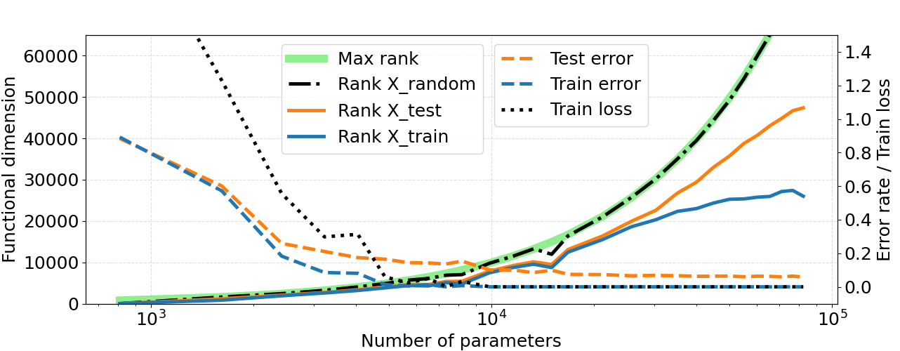
Figure 3: Behavior of different complexity measures as the size of the network increases. The values of the several ranks are to be read on the left axis, titled ‘functional dimension’. The values for the test and train errors and the train loss are to be read on the right axis.

The results of the experiment are in Figure 3. When increasing the number of parameters, the train loss, the train error and the test error decrease. For $w\geq 12$, i.e. when the number of parameters is superior or equal to $9\,862$, the train error is equal to $0$: the network is able to fit perfectly the training images. However, the test error continues to decrease even after the train error reaches $0$: from $0.101$ when $w=12$ to $0.058$ when $w=85$.

As we can see, the quantity $\mathrm{rank}{\left(\mathbf{D}f_{\theta}(X_{\text{random}})\right)}$ in the case of the $40\,000$ inputs generated as Gaussian vectors, $X_{\text{random}}$, is nearly always equal to its maximum theoretical value Max_rank. This indicates first that $r^{*}(\theta)$ is equal to its maximal theoretical value, and second that $\mathrm{rank}{\left(\mathbf{D}f_{\theta}(X_{\text{random}})\right)}$ provides here a good estimation of $r^{*}(\theta)$. Furthermore, according to Bona-Pellissier u. a. (2022), the networks parameters are locally identifiable from $X_{\text{random}}$ in this case.

The ranks $\mathrm{rank}{\left(\mathbf{D}f_{\theta}(X_{\text{train}})\right)}$ and $\mathrm{rank}{\left(\mathbf{D}f_{\theta}(X_{\text{test}})\right)}$ are nearly equal when the number of parameters is smaller than $21\,185$ ($w=25$). For these sizes, it seems to indicate that $\mathrm{rank}{\left(\mathbf{D}f_{\theta}(X_{\text{test}})\right)}$ is indeed equal to the functional dimension over the distribution of inputs, and that $\mathrm{rank}{\left(\mathbf{D}f_{\theta}(X_{\text{train}})\right)}$ already attains it, which means that adding MNIST images to $X_{\text{train}}$ would not increase $\mathrm{rank}{\left(\mathbf{D}f_{\theta}(X_{\text{train}})\right)}$. It thus also suggests that the functional dimension over the distribution of inputs (the MNIST images) is smaller than $r^{*}(\theta)$ which consider all $X$ inside but also outside of this distribution, and which, as we have seen in the previous paragraph, is maximal here. In the light of Bona-Pellissier u. a. (2022), this also shows that $\theta$ is not locally identifiable from $X_{\text{train}}$ nor $X_{\text{test}}$. This suggests that for these networks and the MNIST dataset, using only samples of the input distribution does not allow to identify the parameters of a network, and one needs to add examples outside the input distribution.

Then, for more than $21\,185$ parameters, a gap appears between the two ranks $\mathrm{rank}{\left(\mathbf{D}f_{\theta}(X_{\text{train}})\right)}$ and $\mathrm{rank}{\left(\mathbf{D}f_{\theta}(X_{\text{test}})\right)}$, i.e. $\mathrm{rank}{\left(\mathbf{D}f_{\theta}(X_{\text{train}})\right)}$ is smaller than the functional dimension over the distribution of the inputs. Furthermore, while both ranks are not far from the maximum rank for small numbers of parameters, the gap increases with the number of parameters, to the point where the shape of the curves seem to diverge: while the maximum rank is nearly proportional to the number of parameters, the ranks $\mathrm{rank}{\left(\mathbf{D}f_{\theta}(X_{\text{train}})\right)}$ and $\mathrm{rank}{\left(\mathbf{D}f_{\theta}(X_{\text{test}})\right)}$ seem to increase less and less with the number of parameters. This is the consequence of the geometry-induced implicit regularization described in Section 4.2 and Figure 2. The regularization on the training sample seems to also concern the input distribution in general as the curve $\mathrm{rank}{\left(\mathbf{D}f_{\theta}(X_{\text{test}})\right)}$ indicates.

7.3 Behavior of the Functional Dimensions During Training

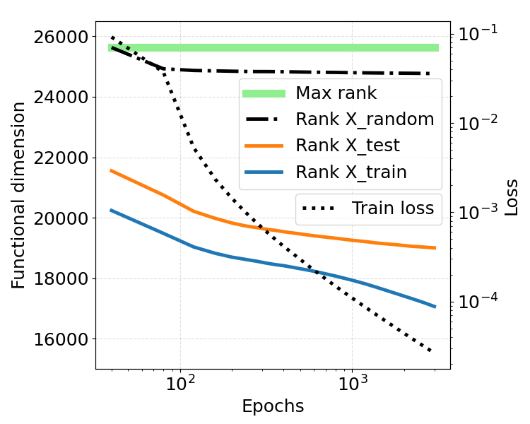
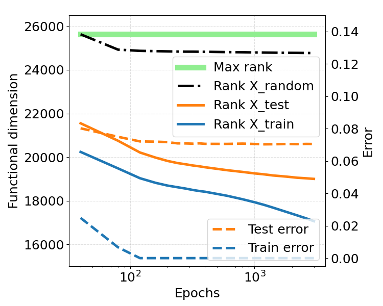
Figure 4: Behavior of different complexity measures during training. The values of the different ranks are to be read on the left axis, titled ‘functional dimension’. The values of the train loss (on the left figure), and the values of the test and train errors (on the right figure) are to be read on the right axis.

We consider the setting described in Section 7.1, where we fix the value of $w$ to $30$. For this experiment, we keep the original MNIST images and labels in $(X_{\text{train}},Y_{\text{train}})$ and $(X_{\text{test}},Y_{\text{test}})$ and we set the size of the random set $X_{\text{random}}$ to $20\,000$. The architecture is $(784,30,30,30,10)$, which corresponds to a total number of parameters equal to $25\,720$. The quantities plotted in the previous experiment (see Figure 3) are computed after the training is done. In contrast, here, we fix a total number of epoch to $3\,000$ and we compute the same quantities during training, throughout the epochs.

More precisely, we study the quantities Max rank, Rank X_random, Rank X_test, Rank X_train, Train loss, Test error and Train error, as described in Section 7.1. They are computed at the epochs $\{40,80,120,160,200,240,280,320,360,400\}\cup\{600,800,1000,1200,1400\}\cup\{1800,2200,2600,3000\}$. We plot these quantities in Figure 4.

We plot the train loss (on the left), which decreases throughout the epochs, and the train error (on the right), which decreases and reaches $0$ at epoch $120$, after which all training images are always correctly classified. The test error decreases the most in the first 80 epochs, after which it continues to decrease, although at a slower pace.

At the beginning of the training, the quantity $\mathrm{rank}{\left(\mathbf{D}f_{\theta}(X_{\text{random}})\right)}$ is equal to the maximum rank, here equal to $25\,630$, and it decreases to reach $24\,769$ at the end of the training. As can be seen in the experiments of Sections 7.2, 7.4 and 7.5, most of the time, at the end of the training, $\mathrm{rank}{\left(\mathbf{D}f_{\theta}(X_{\text{random}})\right)}$ is equal or very close to the maximum rank, but sometimes, there is a small gap between both quantities. The training studied here corresponds to one of the latter cases. As shown by Bona-Pellissier u. a. (2022), when $\mathrm{rank}{\left(\mathbf{D}f_{\theta}(X_{\text{random}})\right)}$ is maximal, the parameterization $\theta$ is locally identifiable from the sample $X_{\text{random}}$. On the contrary, the gap observed here at the end of the training indicates some lack of identifiability from $X_{\text{random}}$.

We observe that the value of $\mathrm{rank}{\left(\mathbf{D}f_{\theta}(X_{\text{train}})\right)}$ consistently decreases during training. Such a behavior is consistent with the geometric interpretation of Section 4.2 and 4.3, and Figure 2. The value of $\mathrm{rank}{\left(\mathbf{D}f_{\theta}(X_{\text{test}})\right)}$ also decreases, with a more gentle slope. This indicates that the geometry-induced implicit regularization occurring on the training sample is ‘communicated’ to the test sample.

7.4 Behavior of the Functional Dimensions when $X$ is Corrupted

We consider the same setting as the experiments of Section 7.1, with $w=30$, which corresponds to a total number of parameters equal to $25\,720$.

The network is trained, during $3\,000$ epochs, repeatedly over different train sets of size $6\,000$ made of MNIST images. We add to the train images a Gaussian noise, before clipping the values of the pixels between $0$ and $1$, to stay consistent with black and white images. We do the same for the test images. This blurs the input distribution. For each training, we use a different noise variance, which overall varies between $10^{-3}$ and $1$. We represent visually an image with different levels of noise in Figure 5. The network is trained to the point it is able to interpolate the training examples: for all the settings, the final train error is equal to $0$.

Figure 5: Effect of the noise on a MNIST image for different amplitudes. From left to right, a MNIST image to which has been added a Gaussian noise, of amplitude $10^{-2},10^{-1},5\times 10^{-1}$ and $10^{0}$ respectively.

Once the training is done, we compute the quantities Max rank, Rank X_random, Rank X_test, Rank X_train, Test error, and Train error described in Section 7.1, for the different noise levels. The size of $X_{\text{random}}$ is $20\,000$. We plot these quantities in Figure 6.

As already said, the expressiveness of the network permits to fit the learning data perfectly. The training error is zero for all noise levels. However, the noise has two effects: an effect on the distribution of inputs which becomes more complex, and an effect on the difficulty of the problem. Indeed, as is reflected by the increase in the test error, the problem becomes more difficult. The curve representing $\mathrm{rank}{\left(\mathbf{D}f_{\theta}(X_{\text{train}})\right)}$ also increases, and gets close to the maximum rank for a noise amplitude getting close to $1$. This phenomenon is coherent with the fact that the batch functional dimension is linked to activation patterns, which are linked to the distribution of the inputs, which –as already said– are made more complex by the noise. The quantity $\mathrm{rank}{\left(\mathbf{D}f_{\theta}(X_{\text{test}})\right)}$ also increases, but for smaller noises than $X_{\text{train}}$. It oscillates close to the maximum rank.

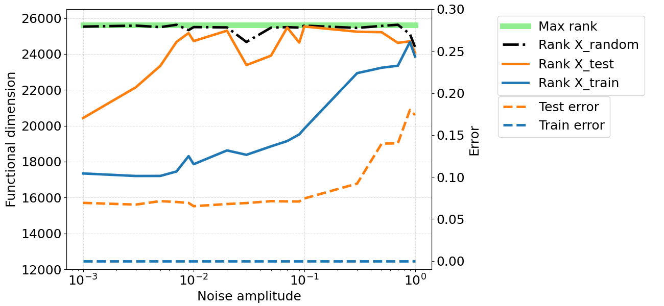
Figure 6: Behavior of different complexity measures when noise is added to the input images. The values of $\mathrm{rank}{\left(\mathbf{D}f_{\theta}(X_{\text{train}})\right)}$ are to be read on the left axis, titled ‘functional dimension’. The values of the test and train errors are to be read on the right axis.

7.5 Behavior of the Functional Dimensions when $Y$ is Corrupted

We consider the setting described in Section 7.1, for three different values of $w$, equal to $30$, $50$ and $60$ respectively. The first experiment carried out was the one with the width $w=30$, in harmony with the experiments of Sections 7.3 and 7.4, and we then added the cases $w=50$ and $w=60$ to see the impact of the width on this experiment.

Following Neyshabur u. a. (2017); Zhang u. a. (2021), we study what happens when part of the labels of the training set are corrupted with random labels. The network is trained repeatedly over different train sets of size $6\,000$ made of MNIST images. A varying number of the labels associated with the training images are set to a random value, according to the uniform distribution over $\{0,1,\ldots,9\}$. The quantity of images with random labels varies from $0$ to $4\,500$. Each time, the network is trained to the point where it interpolates the training set, even with the random labels.

Intuitively, the more corrupted labels there are, the more complex the function interpolating the training data should be. The distribution of the inputs is however the same and it is not clear if the linear regions, defined by the activation patterns, and used to describe the interpolating function need to change much when corruption increases. Another interpretation is that depending on the level of corruption, we select different global minimizers of the empirical risk with respect to the $1500$ images that always remain clean. The purpose of this experiment is to see if the functional dimension increases with the proportion of corrupted labels and the test error, when $w$ is such that implicit regularization occurs.

The quantities Max_rank, Rank_X_random, Rank_X_test, Rank_X_train, Train loss, Test error and Train error are described in Section 7.1. We plot these quantities as a function of the number of corrupted labels in Figure 7 for three different values of $w$. The case $w=30$, is described in Section 7.5.1, and the case $w=50$ is described in Section 7.5.2.

7.5.1 Observations when $w=30$

Consistently with Sections 7.3 and 7.4, we take $w=30$, which corresponds to a number of parameters equal to $25\,720$. The size of the test set $X_{\text{test}}$ and of the random Gaussian inputs $X_{\text{random}}$ are both equal to $20\,000$. The learning performs $3\,000$ epochs. The plots associated to this experiment correspond to the left side of Figure 7.

As expected, the test error (the proportion of images in $X_{\text{test}}$ that are misclassified) increases with the number of corrupted labels: from $0.08$ when no label is corrupted to $0.73$ when $4500$ images out of $6000$ have random labels.

In this experiment, again, we observe that $\mathrm{rank}{\left(\mathbf{D}f_{\theta}(X_{\text{random}})\right)}$ is often equal to the maximum rank, which is here equal to $25630$. For numbers of corrupted labels equal to $500$ and $1500$, we observe that the value is slightly lower.

Although we can observe a clear increase of the ranks $\mathrm{rank}{\left(\mathbf{D}f_{\theta}(X_{\text{train}})\right)}$ and $\mathrm{rank}{\left(\mathbf{D}f_{\theta}(X_{\text{test}})\right)}$ between $0$ and $500$ corrupted labels, for a greater number of corrupted labels these quantities are relatively stable and do not seem to be much affected by the corruption of the labels. We try to clarify this observation by performing two other experiments with a bigger width $w$ in the following section.

7.5.2 Observations when $w=50$ and $w=60$

To better understand the impact of label corruption on the functional dimension, we repeat the previous experiment twice, this time with widths $w$ set to $50$ and $60$, corresponding to a number of parameters equal to $44860$ and $55030$ respectively. This corresponds to points on the right of curve on fig. 3, where implicit regularization occurs the most. We keep the sizes of $X_{\text{train}}$ and $X_{\text{test}}$ to $6000$ and $20000$ respectively, and we increase the size of $X_{\text{random}}$ to $40000$. The plots associated with this experiment correspond to the right side of Figure 7.

We observe similar train and test errors as in 7.5.1. We also observe similarly that $\mathrm{rank}{\left(\mathbf{D}f_{\theta}(X_{\text{random}})\right)}$ is often equal to the maximum rank (but note that we increase the size of $X_{\text{random}}$ here).

For these two widths, the increase of both quantities $\mathrm{rank}{\left(\mathbf{D}f_{\theta}(X_{\text{train}})\right)}$ and $\mathrm{rank}{\left(\mathbf{D}f_{\theta}(X_{\text{test}})\right)}$ is clearer, in particular in the case of $X_{\text{train}}$.

Overall, the experiments 7.5.1 and 7.5.2 indicate that there is a positive correlation between the functional dimensions and the complexity of the function learned by the neural network.

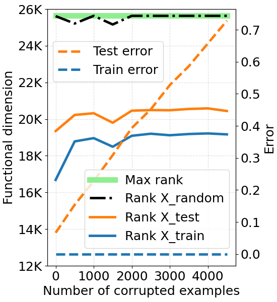
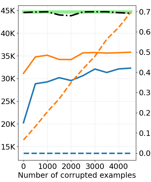
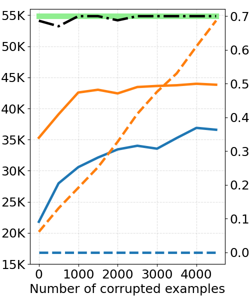
Figure 7: Behavior of different complexity measures as some corrupted labels are introduced in the training set, tested for three network widths. The values of the different ranks are to be read on the left axis, titled ‘functional dimension’. The values of the test and train errors are to be read on the right axis. Width of the network from left to right: $w=30$, $w=50$ and $w=60$.

8 Conclusion and perspectives

In this article, we describe the local geometry of deep ReLU neural networks. The study shows that the image of a sample $X$ by deep ReLU neural networks of a fixed architecture is a set whose local dimension varies. The local dimension is called the batch functional dimension by Grigsby u. a. (2022). We show that the parameter space is divided into pieces where the batch functional dimension is fixed. Empirically, the pieces of small dimensions are on the outside of the ones of large dimensions. They are favored by the optimization. We call this phenomenon geometry-induced implicit regularization. When $X$ is allowed to vary, we also study the maximal dimension over all possible $X$. We call it the computable full functional dimension. Both notions of local complexity are determined by the activation patterns. We investigate the practical computation of the functional dimensions and provide experiments emphasizing the geometry-induced implicit regularization and the link between functional dimensions and the complexity of the learning task.

This opens up many perspectives in deep learning theory. The formal connection between the notions of local complexity and the generalization gap is still missing. It would permit us to obtain a theory that explains the good performance of deep learning. It would be interesting to study more systematically how the functional dimensions of the learned parameters depend on the distribution of the learned phenomenon. To do so, it would be interesting to study instances in larger dimensions. Algorithms of a better complexity for computing the functional dimensions are needed. In particular, since we have proved that the batch functional dimension is almost-surely determined by the activation patterns, it would be interesting to compute the former using the activation patterns instead of the gradients.

Appendix A Proofs of Section 3

This appendix is devoted to the proofs of Section 3. In Section A.1, we prove Theorem 1, and in Section A.2 we prove Proposition 2.

A.1 Proof of Theorem 1

Let us define, for $\ell\in\llbracket 1,L-1\rrbracket$ and $v\in V_{\ell}$ the set

$$\mathcal{T}_{v}=\Bigg{\{}(x,\theta)\in\mathbb{R}^{N_{0}}\times(\mathbb{R}^{E}\times\mathbb{R}^{B})~{}|~{}\sum_{v^{\prime}\in V_{\ell-1}}w_{v^{\prime}\to v}\left(f_{\theta}^{\ell-1}(x)\right)_{v^{\prime}}+b_{v}=0\Bigg{\}},$$ (24)

and let

$$\mathcal{T}=\cup_{\ell=1}^{L-1}\cup_{v\in V_{\ell}}\mathcal{T}_{v}.$$ (25)

Similarly, for any $x\in\mathbb{R}^{N_{0}}$, $\ell\in\llbracket 1,L-1\rrbracket$ and $v\in V_{\ell}$, we define the set

$$\mathcal{T}^{x}_{v}=\Bigg{\{}\theta\in\mathbb{R}^{E}\times\mathbb{R}^{B}~{}|~{}\sum_{v^{\prime}\in V_{\ell-1}}w_{v^{\prime}\to v}\left(f_{\theta}^{\ell-1}(x)\right)_{v^{\prime}}+b_{v}=0\Bigg{\}},$$

and let

$$\mathcal{T}^{x}=\cup_{\ell=1}^{L-1}\cup_{v\in V_{\ell}}\mathcal{T}_{v}^{x}.$$

Lemma 12.

• • Over $\mathbb{R}^{N_{0}}\times(\mathbb{R}^{E}\times\mathbb{R}^{B})$, the function $(x,\theta)\longmapsto a(x,\theta)\in\{0,1\}^{N_{1}+\cdots+N_{L-1}}$ takes exactly $2^{N_{1}+\dots+N_{L-1}}$ distinct values.

  • For any $\delta\in\{0,1\}^{N_{1}+\cdots+N_{L-1}}$, we write

    $$A_{\delta}=\{(x,\theta)\in\mathbb{R}^{N_{0}}\times(\mathbb{R}^{E}\times\mathbb{R}^{B})~{}|~{}a(x,\theta)=\delta\},$$ (26)

    which is thus nonempty. Then: On $A_{\delta}$, the function $(x,\theta)\longmapsto f_{\theta}(x)$ is analytic.

  • The set $\mathcal{T}$ has Lebesgue measure zero and $\cup_{\delta\in\{0,1\}^{N_{1}+\cdots+N_{L-1}}}\partial A_{\delta}=\mathcal{T}$. Therefore, for any $\delta\in\{0,1\}^{N_{1}+\cdots+N_{L-1}}$, $\partial A_{\delta}$ is a closed set of Lebesgue measure zero in $\mathbb{R}^{N_{0}}\times(\mathbb{R}^{E}\times\mathbb{R}^{B})$.

• • For any fixed $x\in\mathbb{R}^{N_{0}}$, the function $\theta\longmapsto a(x,\theta)$ exactly takes $2^{N_{1}+\dots+N_{L-1}}$ distinct values.

  • For $x\in\mathbb{R}^{N_{0}}$ and $\delta\in\{0,1\}^{N_{1}+\cdots+N_{L-1}}$, we write

    $$A^{x}_{\delta}=\{\theta\in\mathbb{R}^{E}\times\mathbb{R}^{B}~{}|~{}a(x,\theta)=\delta\}.$$

    Then: On $A^{x}_{\delta}$, the function $\theta\longmapsto f_{\theta}(x)$ is analytic.

  • The set $\mathcal{T}^{x}$ has Lebesgue measure zero and $\cup_{\delta\in\{0,1\}^{N_{1}+\cdots+N_{L-1}}}\partial A^{x}_{\delta}=\mathcal{T}^{x}$. Therefore, for any $\delta\in\{0,1\}^{N_{1}+\cdots+N_{L-1}}$, $\partial A^{x}_{\delta}$ is a closed set with Lebesgue measure zero in $\mathbb{R}^{E}\times\mathbb{R}^{B}$.

Proof of Lemma 12.

To avoid repetitions, we only detail the proof of $(i)$. The proof of $(ii)$ is very similar, considering functions of $\theta$ only (with $x$ fixed) rather than $(x,\theta)$.

We first prove the first item, i.e. we prove that all activation patterns are reached. The set $\{0,1\}^{N_{1}+\cdots+N_{L-1}}$ is finite and its cardinal is $2^{N_{1}+\dots+N_{L-1}}$. Observe that for any $\delta\in\{0,1\}^{N_{1}+\cdots+N_{L-1}}$, by taking $\theta\in\mathbb{R}^{E}\times\mathbb{R}^{B}$ such that $w_{v\rightarrow v^{\prime}}=0$ for any $(v\rightarrow v^{\prime})\in E$, $b_{v}=0$ for $v\in V_{L}$ and $b_{v}=(-1)^{1+\delta_{v}}$ for any $v\in V_{1}\cup\dots\cup V_{L-1}$, then, for any $x\in\mathbb{R}^{N_{0}}$ and any $v\in V_{1}\cup\dots\cup V_{L-1}$, we have $a_{v}(x,\theta)=\delta_{v}$, i.e. $a(x,\theta)=\delta$.

In order to prove the second item, i.e. that the function $(x,\theta)\longmapsto f_{\theta}(x)$ is analytic, we remind the definition of $f_{\theta}^{\ell}$, in (1), and we define

$$a_{\leq\ell}(x,\theta)=\begin{cases}(a_{v}(x,\theta))_{v\in V_{1}\cup\cdots\cup V_{\ell}}&~{}\text{if}~{}\ell\geq 1,\\ 1&~{}\text{if}~{}\ell=0.\end{cases}$$

We prove by induction that the assertion

$$H_{\ell}:\left\{\begin{array}[]{l}\forall D\subseteq\mathbb{R}^{N_{0}}\times(\mathbb{R}^{E}\times\mathbb{R}^{B}),~{}~{}\text{if $(x,\theta)\longmapsto a_{\leq\ell}(x,\theta)$ is constant on $D$, then }\\ \text{ $(x,\theta)\longmapsto f_{\theta}^{\ell}(x)$ is polynomial on $D$ }\end{array}\right.$$

holds, for all $\ell\in\llbracket 0,L-1\rrbracket$.

The assertion $H_{0}$ indeed holds because $f_{\theta}^{0}(x)=x$ is polynomial in $(x,\theta)$ (of degree $1$) on any subset of $\mathbb{R}^{N_{0}}\times(\mathbb{R}^{E}\times\mathbb{R}^{B})$. Assume now that for some $\ell\in\llbracket 1,L-1\rrbracket$, $H_{\ell-1}$ holds, and let us prove $H_{\ell}$.

Let $D\subseteq\mathbb{R}^{N_{0}}\times(\mathbb{R}^{E}\times\mathbb{R}^{B})$ such that $a_{\leq\ell}(x,\theta)$ is constant on $D$. For $(x,\theta)\in D$ and $v\in V_{\ell}$, using (6), we have

$$\left(f_{\theta}^{\ell}(x)\right)_{v}= a_{v}(x,\theta)\left(\sum_{v^{\prime}\in V_{\ell-1}}w_{v^{\prime}\to v}\left(f_{\theta}^{\ell-1}(x)\right)_{v^{\prime}}+b_{v}\right).$$

The quantity $a_{\leq\ell-1}(x,\theta)$ is constant on $D$ and thus from $H_{\ell-1}$, for all $v^{\prime}\in V_{\ell-1}$, $(x,\theta)\longmapsto(f_{\theta}^{\ell-1}(x))_{v^{\prime}}$ is a polynomial function of $(x,\theta)$ on $D$. Since $a_{v}(x,\theta)$ is constant on $D$, $\left(f_{\theta}^{\ell}(x)\right)_{v}$ is a polynomial function of $(x,\theta)$. This concludes the proof by induction that $H_{\ell}$ holds for all $\ell\in\llbracket 0,L-1\rrbracket$.

If we recall from (1) that $y^{L}_{\theta}(x)\in\mathbb{R}^{N_{L}}$ is the vector satisfying, for all $v\in V_{L}$,

$$(y_{\theta}^{L}(x))_{v}=\sum_{v^{\prime}\in V_{L-1}}w_{v^{\prime}\to v}(f_{\theta}^{L-1}(x))_{v^{\prime}}+b_{v},$$

we have

$$f_{\theta}(x)=\sigma_{L}(y_{\theta}^{L}(x)).$$

We recall the notations $A_{\delta},\delta\in\{0,1\}^{N_{1}+\dots+N_{L-1}}$, in (26). For $\delta\in\{0,1\}^{N_{1}+\dots+N_{L-1}}$, $a_{\leq L-1}(x,\theta)=a(x,\theta)$ is constant on $A_{\delta}$ and thus from $H_{L-1}$, $(x,\theta)\longmapsto f_{\theta}^{L-1}(x)$ is polynomial on $A_{\delta}$. As a consequence, $(x,\theta)\longmapsto y^{L}_{\theta}(x)$ is polynomial on $A_{\delta}$, and since $\sigma_{L}$ is analytic, $(x,\theta)\longmapsto f_{\theta}(x)$ is analytic on $A_{\delta}$. This proves the second item of Lemma 12, $(i)$.

Let us now show the third item, which states that $\mathcal{T}$ has Lebesgue measure zero. For that, let us show that for all $\ell\in\llbracket 1,L-1\rrbracket$ and $v\in V_{\ell}$, $\mathcal{T}_{v}$ has Lebesgue measure zero. To do so, since $\cup_{\delta}A_{\delta}=\mathbb{R}^{N_{0}}\times(\mathbb{R}^{E}\times\mathbb{R}^{B})$, we consider $\ell\in\llbracket 1,L-1\rrbracket$ and $v\in V_{\ell}$, and prove that, for all $\delta\in\{0,1\}^{N_{1}+\dots+N_{L-1}}$, $\mathcal{T}_{v}\cap A_{\delta}$ has Lebesgue measure zero. For $\delta\in\{0,1\}^{N_{1}+\dots+N_{L-1}}$, $a_{\leq\ell-1}(x,\theta)$ is constant on $A_{\delta}$ and thus from $H_{\ell-1}$, $(x,\theta)\longmapsto f_{\theta}^{\ell-1}(x)$ is a polynomial function of $(x,\theta)$ on $A_{\delta}$ and thus $\sum_{v^{\prime}\in V_{\ell-1}}w_{v^{\prime}\to v}\left(f_{\theta}^{\ell-1}(x)\right)_{v^{\prime}}+b_{v}$ also is. Since the variable $(x,\theta)\mapsto b_{v}$ is not present in the expression of $f_{\theta}^{\ell-1}(x)$, it only appears in a single monomial of degree and coefficient $1$ of $\sum_{v^{\prime}\in V_{\ell-1}}w_{v^{\prime}\to v}\left(f_{\theta}^{\ell-1}(x)\right)_{v^{\prime}}+b_{v}$. The latter polynomial function is therefore non-constant. Hence the set $\mathcal{T}_{v}\cap A_{\delta}$, constituted by the zeros of this polynomial function, has Lebesgue measure zero. Since $\cup_{\delta}A_{\delta}=\mathbb{R}^{N_{0}}\times(\mathbb{R}^{E}\times\mathbb{R}^{B})$, we finally conclude that, for any $\ell\in\llbracket 1,L-1\rrbracket$ and $v\in V_{\ell}$, $\mathcal{T}_{v}$ has Lebesgue measure zero.

The set

$$\mathcal{T}=\cup_{\ell=1}^{L-1}\cup_{v\in V_{\ell}}\mathcal{T}_{v}$$

is thus also of Lebesgue measure zero.

Let us now prove the set equality:

$$\bigcup_{\delta}\partial A_{\delta}=\mathcal{T}.$$ (27)

We first show the inclusion $\bigcup_{\delta}\partial A_{\delta}\subseteq\mathcal{T}$. Consider $\delta\in\{0,1\}^{N_{1}+\dots+N_{L-1}}$ and let us now show that $\partial A_{\delta}\subseteq\mathcal{T}$. To do so, consider $(x,\theta)\in\partial A_{\delta}$. Since $(x,\theta)\not\in\operatorname{Int}(A_{\delta})$, for any $\varepsilon$ there exists $\delta_{\varepsilon}\neq\delta$ such that $B((x,\theta),\varepsilon)\cap A_{\delta_{\varepsilon}}\neq\emptyset$. Since the set of all possible $\delta_{\varepsilon}$ is finite, we are sure that there exists $\delta^{\prime}\neq\delta$ such that $(x,\theta)\in\overline{A}_{\delta^{\prime}}$. Let $\ell\in\llbracket 1,L-1\rrbracket$ and $v\in V_{\ell}$ such that $\delta_{v}\neq\delta^{\prime}_{v}$. We assume without loss of generality that $\delta_{v}=0$. The proof is indeed similar when $\delta_{v}=1$. There exists $(x_{n},\theta_{n})\in A_{\delta}^{\mathbb{N}^{*}}$ such that $(x_{n},\theta_{n})\to(x,\theta)$ as $n\to\infty$ and there exists $(x^{\prime}_{n},\theta^{\prime}_{n})\in A_{\delta^{\prime}}^{\mathbb{N}^{*}}$ such that $(x^{\prime}_{n},\theta^{\prime}_{n})\to(x,\theta)$ as $n\to\infty$. We have $a_{v}(x_{n},\theta_{n})=0$ and $a_{v}(x^{\prime}_{n},\theta^{\prime}_{n})=1$ for all $n$.

Using that $(x,\theta)\longmapsto\sum_{v^{\prime}\in V_{\ell-1}}w_{v^{\prime}\to v}\left(f_{\theta}^{\ell-1}(x)\right)_{v^{\prime}}+b_{v}$ is continuous and taking the limit of this function at $(x_{n},\theta_{n})$, as $n$ goes to infinity, we obtain that $\sum_{v^{\prime}\in V_{\ell-1}}w_{v^{\prime}\to v}\left(f_{\theta}^{\ell-1}(x)\right)_{v^{\prime}}+b_{v}\leq 0$. Reasoning similarly with the sequence $(x^{\prime}_{n},\theta^{\prime}_{n})_{n\in\mathbb{N}^{*}}$ we obtain the reverse inequality and conclude that $\sum_{v^{\prime}\in V_{\ell-1}}w_{v^{\prime}\to v}\left(f_{\theta}^{\ell-1}(x)\right)_{v^{\prime}}+b_{v}=0$. This shows that $(x,\theta)\in\mathcal{T}_{v}\subseteq\mathcal{T}$. This finishes the proof of $\partial A_{\delta}\subseteq\mathcal{T}$.

Let us now show the reciprocal inclusion $\mathcal{T}\subseteq\bigcup_{\delta}\partial A_{\delta}$. Indeed, let $(x,\theta)\in\mathcal{T}$. There exist $\ell\in\llbracket 1,L-1\rrbracket$ and $v\in V_{\ell}$ such that $(x,\theta)\in\mathcal{T}_{v}$. There also exists $\delta\in\{0,1\}^{N_{1}+\dots+N_{L-1}}$ such that $(x,\theta)\in A_{\delta}.$ In particular, since $\sum_{v^{\prime}\in V_{\ell-1}}w_{v^{\prime}\to v}\left(f_{\theta}^{\ell-1}(x)\right)_{v^{\prime}}+b_{v}=0$, we have $\delta_{v}=a_{v}(x,\theta)=1$. For any $\varepsilon>0$, by replacing $b_{v}$ by $b_{v}-\varepsilon$, we obtain a $\theta_{\varepsilon}$ satisfying $\|\theta-\theta_{\varepsilon}\|\leq\varepsilon$ and $a_{v}(x,\theta_{\varepsilon})=0\neq\delta_{v}$, which shows $(x,\theta_{\varepsilon})\not\in A_{\delta}$. This shows $(x,\theta)\in\partial A_{\delta}\subseteq\bigcup_{\delta}\partial A_{\delta}$. This shows the desired inclusion, and thus the equality (27).

For all $\delta\in\{0,1\}^{N_{1}+\dots+N_{L-1}}$, $\partial A_{\delta}$ is closed by definition of a boundary. Since $\mathcal{T}$ has been shown to have Lebesgue measure zero, then $\partial A_{\delta}$ has Lebesgue measure zero and thus the proof of the part $(i)$ is concluded. ∎

We state and prove another lemma before proving 1. The lemma resembles 1 but does not include the statements on $\mathrm{rank}{\left(\mathbf{D}f_{\theta}(X)\right)}$.

For $n\in\mathbb{N}^{*}$, recalling the definition $\mathcal{T}$ in (25), let us now define

$$\mathcal{T}_{n}=\cup_{i=1}^{n}\left\{\left.(X,\theta)\in\mathbb{R}^{N_{0}\times n}\times(\mathbb{R}^{E}\times\mathbb{R}^{B})\ \right|\ (x^{(i)},\theta)\in\mathcal{T}\right\}.$$ (28)

Similarly, for $n\in\mathbb{N}^{*}$ and $X\in\mathbb{R}^{N_{0}\times n}$, we define

$$\mathcal{T}^{X}=\cup_{i=1}^{n}\left\{\theta\in\mathbb{R}^{E}\times\mathbb{R}^{B}~{}|~{}(x^{(i)},\theta)\in\mathcal{T}\right\}.$$

Lemma 13.

• For all $n\in\mathbb{N}^{*}$, the sets $\widetilde{\mathcal{O}}^{n}_{1},\ldots,\widetilde{\mathcal{O}}^{n}_{{m_{n}}}$ defined in (7) are non-empty, open and disjoint, and they satisfy

  • $\left(\cup_{j=1}^{{m_{n}}}\widetilde{\mathcal{O}}^{n}_{j}\right)^{c}=\mathcal{T}_{n}$, and in particular the complement $\left(\cup_{j=1}^{{m_{n}}}\widetilde{\mathcal{O}}^{n}_{j}\right)^{c}$ is a closed set with Lebesgue measure zero;

  • for all $j\in\llbracket 1,{m_{n}}\rrbracket$, the function $(X,\theta)\longmapsto a(X,\theta)$ is constant on each $\widetilde{\mathcal{O}}^{n}_{j}$ and takes ${m_{n}}$ distinct values on $\cup_{j=1}^{m_{n}}\widetilde{\mathcal{O}}^{n}_{j}$;

  • for all $j\in\llbracket 1,{m_{n}}\rrbracket$, $(X,\theta)\longmapsto f_{\theta}(X)$ is an analytic function on $\widetilde{\mathcal{O}}^{n}_{j}$.

• For all $n\in\mathbb{N}^{*}$, for all $X\in\mathbb{R}^{N_{0}\times n}$, the sets $\widetilde{\mathcal{U}}^{X}_{1},\ldots,\widetilde{\mathcal{U}}^{X}_{{p_{X}}}$ defined in (10) are non-empty, open and disjoint, and they satisfy

  • $\left(\cup_{j=1}^{{p_{X}}}\widetilde{\mathcal{U}}^{X}_{j}\right)^{c}=\mathcal{T}^{X}$, and in particular the complement $\left(\cup_{j=1}^{{p_{X}}}\widetilde{\mathcal{U}}^{X}_{j}\right)^{c}$ is a closed set with Lebesgue measure zero;

  • for all $j\in\llbracket 1,{p_{X}}\rrbracket$, the function $\theta\longmapsto a(X,\theta)$ is constant on each $\widetilde{\mathcal{U}}^{X}_{j}$ and takes ${p_{X}}$ distinct values on $\cup_{j=1}^{p_{X}}\widetilde{\mathcal{U}}^{X}_{j}$;

  • for all $j\in\llbracket 1,{p_{X}}\rrbracket$, $\theta\longmapsto f_{\theta}(X)$ is an analytic function on $\widetilde{\mathcal{U}}^{X}_{j}$.

Proof of Lemma 13.

As in the proof of 12, the proofs of $(i)$ and $(ii)$ are very similar. To avoid repetitions, we only detail the proof of $(i)$.

By definition, see (7), the sets $\widetilde{\mathcal{O}}^{n}_{1},\ldots,\widetilde{\mathcal{O}}^{n}_{{m_{n}}}$ are non-empty, open and disjoint. Before proving the first point of $(i)$, let us notice that $\mathcal{T}_{n}$ is of Lebesgue measure zero. Indeed, the third item of Lemma 12 states that $\mathcal{T}$ has Lebesgue measure zero, and therefore, we see in the definition (28) that $\mathcal{T}_{n}$ is a finite union of zero-measured sets, which shows that it itself has Lebesgue measure zero. Let us also write the following useful characterization: thanks to the characterization of $\mathcal{T}$ in the third item of Lemma 12 $(i)$, we have

$$\mathcal{T}_{n}=\cup_{i=1}^{n}\cup_{\delta\in\{0,1\}^{N_{1}+\dots+N_{L-1}}}\left\{(X,\theta)\in\mathbb{R}^{N_{0}\times n}\times(\mathbb{R}^{E}\times\mathbb{R}^{B})~{}|~{}(x^{(i)},\theta)\in\partial A_{\delta}\right\}.$$ (29)

Let us now show the first point of $(i)$. Let us prove that $(\cup_{j=1}^{{m_{n}}}\widetilde{\mathcal{O}}^{n}_{j})^{c}=\mathcal{T}_{n}$.

To do so, let us first show that $(\cup_{j=1}^{{m_{n}}}\widetilde{\mathcal{O}}^{n}_{j})^{c}\subseteq\mathcal{T}_{n}$. Let $(X,\theta)\in(\cup_{j=1}^{{m_{n}}}\widetilde{\mathcal{O}}^{n}_{j})^{c}$. Consider the $\Delta^{n}_{1},\dots,\Delta^{n}_{q}$ defined just before (7). There exists $j\in\llbracket 1,q\rrbracket$ such that $a(X,\theta)=\Delta^{n}_{j}$. Since $(X,\theta)\not\in\widetilde{\mathcal{O}}^{n}_{j}$, there exists a sequence $(X_{k},\theta_{k})_{k\in\mathbb{N}^{*}}$ such that $(X_{k},\theta_{k})\rightarrow(X,\theta)$, as $k\rightarrow\infty$ and $a(X_{k},\theta_{k})\neq\Delta^{n}_{j}$, for all $k$. Modulo the extraction of a sub-sequence, we can assume that there exist $i\in\llbracket 1,n\rrbracket$ such that for all $k\in\mathbb{N}^{*}$, $a(x_{k}^{(i)},\theta_{k})\neq\delta$, where $x_{k}^{(i)}$ is the $i^{th}$ column of $X_{k}$, and where we denote $\delta=(\Delta^{n}_{j})_{i}$. Thus, we have $(x_{k}^{(i)},\theta_{k})\not\in A_{\delta}$, for all $k$, and since $(x^{(i)},\theta)\in A_{\delta}$, we conclude $(x^{(i)},\theta)\in\partial A_{\delta}$. The characterization (29) thus shows $(X,\theta)\in\mathcal{T}_{n}$. This shows $(\cup_{j=1}^{{m_{n}}}\widetilde{\mathcal{O}}^{n}_{j})^{c}\subseteq\mathcal{T}_{n}$.

Let us now show that $\mathcal{T}_{n}\subseteq(\cup_{j=1}^{{m_{n}}}\widetilde{\mathcal{O}}^{n}_{j})^{c}$. If $(X,\theta)\in\mathcal{T}_{n}$, there exists $i\in\llbracket 1,n\rrbracket$ and $\delta\in\{0,1\}^{N_{1}+\dots+N_{L-1}}$ such that $(x^{(i)},\theta)\in\partial A_{\delta}$. Thus, for any $\varepsilon>0$, $(x,\theta^{\prime})\longmapsto a(x,\theta^{\prime})$ is not constant over $B((x^{(i)},\theta),\varepsilon)$. As a consequence, $(X,\theta)$ does not belong to any of the open sets $\widetilde{\mathcal{O}}_{j^{\prime}}^{n}$.

This shows $(\cup_{j=1}^{{m_{n}}}\widetilde{\mathcal{O}}^{n}_{j})^{c}=\mathcal{T}_{n}$, and thus, since $\mathcal{T}_{n}$ is of Lebesgue measure zero, $(\cup_{j=1}^{{m_{n}}}\widetilde{\mathcal{O}}^{n}_{j})^{c}$ has Lebesgue measure zero. Adding that the complement of an open set is closed, $(\cup_{j=1}^{{m_{n}}}\widetilde{\mathcal{O}}^{n}_{j})^{c}$ is closed, which ends the proof of the first point of $(i)$.

The second point of $(i)$ holds by definition of $\widetilde{\mathcal{O}}^{n}_{1},\ldots,\widetilde{\mathcal{O}}^{n}_{{m_{n}}}$.

Let us now show the third point of $(i)$. Let $j\in\llbracket 1,{m_{n}}\rrbracket$. The function $(X,\theta)\longmapsto a(X,\theta)$ is constant on $\widetilde{\mathcal{O}}^{n}_{j}$. The set $\widetilde{\mathcal{O}}^{n}_{j}$ is associated to $\Delta^{n}_{j}$ in (7) and the latter is of the form $(\delta^{1},\ldots,\delta^{n})$ with $\delta^{i}\in\{0,1\}^{N_{1}+\dots+N_{L-1}}$ for $i\in\llbracket 1,n\rrbracket$. Fix $i^{\prime}\in\llbracket 1,n\rrbracket$. Then for $X=(x^{(i)})_{i\in\llbracket 1,n\rrbracket}$ with $(X,\theta)\in\widetilde{\mathcal{O}}^{n}_{j}$, $(x^{(i^{\prime})},\theta)\in A_{\delta^{i^{\prime}}}$. Hence, Lemma 12 $(i)$ shows that $f_{\theta}(x^{(i^{\prime})})$ is an analytic function of $(x^{(i^{\prime})},\theta)$ and thus of $(X,\theta)$. The quantity $f_{\theta}(X)$ is a matrix whose columns are $f_{\theta}(x^{(i)})$, $i\in\llbracket 1,n\rrbracket$. Hence $(X,\theta)\longmapsto f_{\theta}(X)$ is an analytic function on $\widetilde{\mathcal{O}}^{n}_{j}$, which concludes the proof of $(i)$. ∎

Proof of Theorem 1.

Again, the proofs of $(i)$ and $(ii)$ are very similar and we only detail the proof of $(i)$.

Consider $n\in\mathbb{N}^{*}$. The sets $\mathcal{O}^{n}_{1},\dots,\mathcal{O}^{n}_{m_{n}}$ are non-empty by definition of $r^{n}_{1},\dots,r^{n}_{m_{n}}$, and they are disjoint because of the inclusion $\mathcal{O}^{n}_{j}\subseteq\widetilde{\mathcal{O}}^{n}_{j}$ for all $j$, and because the sets $\widetilde{\mathcal{O}}^{n}_{1},\ldots,\widetilde{\mathcal{O}}^{n}_{{m_{n}}}$ are disjoint as shown in Lemma 13. Hence the first item holds. The second item is a direct consequence of the definition of $\mathcal{O}^{n}_{j}$, in (9). The third item holds by definition.

To see that $\mathcal{O}^{n}_{j}$ is open, first recall that $\widetilde{\mathcal{O}}^{n}_{j}$ is open, then note that since the function $(X,\theta)\longmapsto f_{\theta}(X)$ is analytic over $\widetilde{\mathcal{O}}^{n}_{j}$ (by Lemma 13 $(i)$), the function $(X,\theta)\longmapsto\mathbf{D}f_{\theta}(X)$ is continuous over $\widetilde{\mathcal{O}}^{n}_{j}$. Since the rank is lower semicontinuous, if $\mathrm{rank}{\left(\mathbf{D}f_{\theta}(X)\right)}=r^{n}_{j}$, then there exists $\epsilon>0$ such that for any $(X^{\prime},\theta^{\prime})\in B((X,\theta),\epsilon)$, we have $\mathrm{rank}{\left(\mathbf{D}f_{\theta^{\prime}}(X^{\prime})\right)}\geq r^{n}_{j}$, which by maximality of $r^{n}_{j}$, is equivalent to $\mathrm{rank}{\left(\mathbf{D}f_{\theta^{\prime}}(X^{\prime})\right)}=r^{n}_{j}$ and to $(X^{\prime},\theta^{\prime})\in\mathcal{O}^{n}_{j}$. This shows that $\mathcal{O}^{n}_{j}$ is open. Hence Item 4 holds.

Item 6 comes directly from Lemma 13 and from the inclusion $\mathcal{O}^{n}_{j}\subseteq\widetilde{\mathcal{O}}^{n}_{j}$.

To finish the proof, we need to prove Item 5, stating that $\left(\cup_{j=1}^{m_{n}}\mathcal{O}^{n}_{j}\right)^{c}$ is a closed set with Lebesgue measure zero. Let us consider a basis $(e_{1},\ldots,e_{|E|+|B|})$ of $\mathbb{R}^{E}\times\mathbb{R}^{B}$ and a basis $(\varepsilon_{1},\ldots,\varepsilon_{nN_{L}})$ of $\mathbb{R}^{N_{L}\times n}$. For all $X$, let us write $M_{\theta}(X)$ for the matrix of the differential $\mathbf{D}f_{\theta}(X)$ of the function $\theta\longmapsto f_{\theta}(X)$ in these two bases. Then $(X,\theta)\longmapsto M_{\theta}(X)$ is an analytic function on $\widetilde{\mathcal{O}}^{n}_{j}$. Recall the notation $r^{n}_{j}=\max_{(X,\theta)\in\widetilde{\mathcal{O}}^{n}_{j}}\mathrm{rank}{\left(\mathbf{D}f_{\theta}(X)\right)}$, and let $(X^{\prime},\theta^{\prime})\in\widetilde{\mathcal{O}}^{n}_{j}$ such that $\mathrm{rank}{\left(\mathbf{D}f_{\theta^{\prime}}(X^{\prime})\right)}=r^{n}_{j}$. We thus have $\mathrm{rank}{\left(M_{\theta^{\prime}}(X^{\prime})\right)}=r^{n}_{j}$, and thus there exists a sub-matrix $N_{\theta^{\prime}}(X^{\prime})$ of $M_{\theta^{\prime}}(X^{\prime})$, of size $r^{n}_{j}\times r^{n}_{j}$, such that $\det N_{\theta^{\prime}}(X^{\prime})\neq 0$. The function $(X,\theta)\longmapsto M_{\theta}(X)$ is an analytic function on $\widetilde{\mathcal{O}}^{n}_{j}$ and thus $(X,\theta)\longmapsto\det(N_{\theta}(X))$ also is. This latter function is not uniformly zero on $\widetilde{\mathcal{O}}^{n}_{j}$ and thus the set of its zeros, that we write $\mathcal{Y}_{j}$, is a closed set of Lebesgue measure zero (Mityagin, 2020).

For all $(X,\theta)\in\widetilde{\mathcal{O}}^{n}_{j}\setminus\mathcal{Y}_{j}$, we have $\det N_{\theta}(X)\neq 0$ and thus $\mathrm{rank}{\left(N_{\theta}(X)\right)}=r^{n}_{j}$ and thus $\mathrm{rank}{\left(M_{\theta}(X)\right)}\geq r^{n}_{j}$. We also have $\mathrm{rank}{\left(M_{\theta}(X)\right)}=\mathrm{rank}{\left(\mathbf{D}f_{\theta}(X)\right)}\leq r^{n}_{j}$ by definition of $r^{n}_{j}$. Hence $\mathrm{rank}{\left(\mathbf{D}f_{\theta}(X)\right)}=r^{n}_{j}$. This shows $\widetilde{\mathcal{O}}^{n}_{j}\setminus\mathcal{Y}_{j}\subseteq\mathcal{O}^{n}_{j}$.

Finally,

$$\left(\cup_{j=1}^{{m_{n}}}\mathcal{O}^{n}_{j}\right)^{c}= \cap_{j=1}^{{m_{n}}}\left(\mathcal{O}^{n}_{j}\right)^{c}$$

$$\subseteq \cap_{j=1}^{{m_{n}}}\left(\widetilde{\mathcal{O}}^{n}_{j}\setminus\mathcal{Y}_{j}\right)^{c}$$

$$= \cap_{j=1}^{{m_{n}}}\left(\left(\widetilde{\mathcal{O}}^{n}_{j}\right)^{c}\cup\mathcal{Y}_{j}\right)$$

$$\subseteq \cap_{j=1}^{{m_{n}}}\left(\left(\widetilde{\mathcal{O}}^{n}_{j}\right)^{c}\cup\left(\cup_{j^{\prime}=1}^{{m_{n}}}\mathcal{Y}_{j^{\prime}}\right)\right)$$

$$= \left(\cap_{j=1}^{{m_{n}}}\left(\widetilde{\mathcal{O}}^{n}_{j}\right)^{c}\right)\cup\left(\cup_{j=1}^{{m_{n}}}\mathcal{Y}_{j}\right)$$

$$= \left(\cup_{j=1}^{{m_{n}}}\widetilde{\mathcal{O}}^{n}_{j}\right)^{c}\cup\left(\cup_{j=1}^{{m_{n}}}\mathcal{Y}_{j}\right).$$

We know from Lemma 13 that $\left(\cup_{j=1}^{{m_{n}}}\widetilde{\mathcal{O}}^{n}_{j}\right)^{c}$ has Lebesgue measure zero. Also each $\mathcal{Y}_{j}$ has Lebesgue measure zero, thus $\cup_{j=1}^{{m_{n}}}\mathcal{Y}_{j}$ has Lebesgue measure zero. Hence, $\left(\cup_{j=1}^{{m_{n}}}\mathcal{O}^{n}_{j}\right)^{c}$ has Lebesgue measure zero, which concludes the proof of $(i)$ in the theorem. ∎

A.2 Proof of Proposition 2

Let us prove more than Proposition 2. We in fact prove the following proposition. Proposition 2 simply corresponds to the first item, but it is convenient to prove the others items at the same time, which will be useful in the proofs of other results.

Proposition 14.

Consider any deep fully-connected ReLU network architecture $(E,V,\sigma_{L})$. Let $\theta,\widetilde{\theta}\in\mathbb{R}^{E}\times\mathbb{R}^{B}$. Assume $\theta\sim\widetilde{\theta}$. Then for any $n\in\mathbb{N}^{*}$ and $X\in\mathbb{R}^{N_{0}\times n}$:

1. if the differential $\mathbf{D}f_{\theta}(X)$ is well-defined, then the differential $\mathbf{D}f_{\widetilde{\theta}}(X)$ is well-defined, and in that case we have

   $$\mathrm{rank}{\left(\mathbf{D}f_{\widetilde{\theta}}(X)\right)}=\mathrm{rank}{\left(\mathbf{D}f_{\theta}(X)\right)};$$

2. if there exists $j\in\llbracket 1,m_{n}\rrbracket$, such that $(X,\theta)\in\widetilde{\mathcal{O}}_{j}^{n}$, then there exists $j^{\prime}\in\llbracket 1,m_{n}\rrbracket$ such that $(X,\widetilde{\theta})\in\widetilde{\mathcal{O}}_{j^{\prime}}^{n}$;

3. if there exists $j\in\llbracket 1,m_{n}\rrbracket$, such that $(X,\theta)\in\mathcal{O}_{j}^{n}$, then there exists $j^{\prime}\in\llbracket 1,m_{n}\rrbracket$ such that $(X,\widetilde{\theta})\in\mathcal{O}_{j^{\prime}}^{n}$.

Proof.

Let $\widetilde{\theta}\sim\theta$, let $n\in\mathbb{N}^{*}$ and let $X\in\mathbb{R}^{N_{0}\times n}$. Let us prove the three items of the proposition.

Let us prove the first item. By definition of the relation $\sim$, in Section 2, there is an invertible linear map $M:\mathbb{R}^{E}\times\mathbb{R}^{B}\longrightarrow\mathbb{R}^{E}\times\mathbb{R}^{B}$ such that $\widetilde{\theta}=M\theta$. Note that when expressed in the canonical basis of $\mathbb{R}^{E}\times\mathbb{R}^{B}$, the matrix corresponding to $M$ is the product of a permutation matrix and a diagonal matrix, with strictly positive diagonal components whose values are given by (4) and (5). Notice that since $M$ corresponds to positive rescalings and neuron permutations, as discussed after (5), we have,

$$\mbox{for any }\theta^{\prime}\in\mathbb{R}^{E}\times\mathbb{R}^{B},\qquad f_{\theta^{\prime}}(X)=f_{M\theta^{\prime}}(X).$$ (30)

Assume that $\mathbf{D}f_{\theta}(X)$ is well-defined, i.e. the map $\theta^{\prime}\mapsto f_{\theta^{\prime}}(X)$ is differentiable at $\theta$. Then, for all $u\in\mathbb{R}^{E}\times\mathbb{R}^{B}$, the following calculation holds, using the fact that $M$ is invertible, using (30) and using (3),

$$f_{\widetilde{\theta}+u}(X)=f_{M\theta+u}(X)= f_{M(\theta+M^{-1}u)}(X)$$

$$= f_{\theta+M^{-1}u}(X)$$

$$= f_{\theta}(X)+\mathbf{D}f_{\theta}(X)(M^{-1}u)+o(\|M^{-1}u\|)$$

$$= f_{\theta}(X)+\mathbf{D}f_{\theta}(X)(M^{-1}u)+o(\|u\|).$$

Hence, $\theta^{\prime}\longmapsto f_{\theta^{\prime}}(X)$ is differentiable at $\widetilde{\theta}$ and for all $u\in\mathbb{R}^{E}\times\mathbb{R}^{B}$,

$$\mathbf{D}f_{\widetilde{\theta}}(X)(u)=\mathbf{D}f_{\theta}(X)(M^{-1}u).$$

Since $M^{-1}$ is invertible, it follows that $\mathrm{rank}{\left(\mathbf{D}f_{\widetilde{\theta}}(X)\right)}=\mathrm{rank}{\left(\mathbf{D}f_{\theta}(X)\right)}$. This concludes the proof of the first item.

Let us now prove the second and the third items. Let $j\in\llbracket 1,m_{n}\rrbracket$ such that $(X,\theta)\in\widetilde{\mathcal{O}}^{n}_{j}$. Again, let us consider the map $M$ defined above. For any $\theta^{\prime}\in\mathbb{R}^{E}\times\mathbb{R}^{B}$, it is well-known (see for instance Bona-Pellissier u. a. 2023a, Proposition 39, Item 2) that since $\theta^{\prime}$ and $M\theta^{\prime}$ are equivalent modulo permutation and positive rescaling, for any $x\in\mathbb{R}^{N_{0}}$, we have $a(x,M\theta^{\prime})=Pa(x,\theta^{\prime})$, for some permutation matrix $P\in\{0,1\}^{(N_{1}+\cdots+N_{L-1})\times(N_{1}+\cdots+N_{L-1})}$ that only depends on $M$ and not on $x$.

Since $(X,\theta)\in\widetilde{\mathcal{O}}^{n}_{j}$, recalling the definition (7), there exists an open neighborhood $\widetilde{U}$ of $(X,\theta)$ such that for any $(X^{\prime},\theta^{\prime})\in\widetilde{U}$, we have $a(X^{\prime},\theta^{\prime})=\Delta^{n}_{j}$. For any $(X^{\prime},\theta^{\prime})\in\widetilde{U}$, we have $a(X^{\prime},M\theta^{\prime})=Pa(X^{\prime},\theta^{\prime})=P\Delta^{n}_{j}$. Furthermore, since $M$ is invertible, the map $\overline{M}$ defined by $(X^{\prime},\theta^{\prime})\mapsto(X^{\prime},M\theta^{\prime})$ is invertible, and the image $\widetilde{V}$ of $\widetilde{U}$ by $\overline{M}$ is thus an open neighborhood of $(X,\widetilde{\theta})$. This shows that there exists $j^{\prime}\in\llbracket 1,m_{n}\rrbracket$ such that $\Delta^{n}_{j^{\prime}}=P\Delta^{n}_{j}$ and $(X,\widetilde{\theta})\in\widetilde{V}\subseteq\widetilde{\mathcal{O}}^{n}_{j^{\prime}}$. This proves the second item.

Finally, if we furthermore assume $(X,\theta)\in\mathcal{O}^{n}_{j}$, applying Theorem 1, we see that the function $(X^{\prime},\theta^{\prime})\longmapsto\mathrm{rank}{\left(\mathbf{D}f_{\theta^{\prime}}(X^{\prime})\right)}$ is locally constant at $(X,\theta)$: there exists an open neighborhood of $(X,\theta)$, $U\subseteq\widetilde{U}$, such that $U\subseteq\mathcal{O}^{n}_{j}$ and thus, for all $(X^{\prime},\theta^{\prime})\in U$, we have $\mathrm{rank}{\left(\mathbf{D}f_{\theta^{\prime}}(X^{\prime})\right)}=r^{n}_{j}$. Thus, applying the invertible map $\overline{M}$, which preserves the rank as shown in the first item, this shows that $(X^{\prime},\theta^{\prime})\longmapsto\mathrm{rank}{\left(\mathbf{D}f_{\theta^{\prime}}(X^{\prime})\right)}$ is also constant on $V=\overline{M}(U)$ (note that $V\subseteq\widetilde{V}$), which is an open set and which contains $(X,\widetilde{\theta})=\overline{M}(X,\theta)$. Since $V\subseteq\widetilde{\mathcal{O}}^{n}_{j^{\prime}}$, this shows that $\mathrm{rank}{\left(\mathbf{D}f_{\widetilde{\theta}}(X)\right)}=r_{j^{\prime}}^{n}$ because $r_{j^{\prime}}^{n}$ is the only value that can be taken on a subset of $\widetilde{\mathcal{O}}^{n}_{j^{\prime}}$ of non-zero Lebesgue measure. In other words, we have $(X,\widetilde{\theta})\in\mathcal{O}^{n}_{j^{\prime}}$ (and in particular we have shown $r^{n}_{j}=r^{n}_{j^{\prime}}$). ∎

Appendix B Calculations for the Example in Section 4.1

We provide in this appendix, the calculations permitting to construct Figure 1. We consider a one-hidden-layer neural network of widths $(1,1,1)$, with the identity activation function on the last layer. To simplify notations, we denote the weights and biases $\theta=(a,b,c,d)\in\mathbb{R}^{4}$ so that $f_{\theta}(x)=b\sigma(ax+c)+d$, for all $x\in\mathbb{R}$. We consider $X=(0,1,2)\in\mathbb{R}^{1\times 3}$ and

$$f_{\theta}(X)^{T}=\left(\begin{array}[]{c}b\sigma(c)+d\\ b\sigma(a+c)+d\\ b\sigma(2a+c)+d\end{array}\right).$$

The boundaries of the sets $\widetilde{\mathcal{U}}_{j}^{X}$, corresponding to the parameters having the same activation pattern, are defined by the equation $c=0$, $a+c=0$ and $2a+c=0$. There are $6$ possible activation patterns corresponding to the zones represented, in the $(a,c)$ plane, on the left of Figure 1.

Since the sets $f_{\widetilde{\mathcal{U}}^{X}_{j}}(X)=\{f_{\theta}(X)~{}|~{}\theta\in\widetilde{\mathcal{U}}^{X}_{j}\}$, for $j\in\llbracket 1,6\rrbracket$, are invariant to translations by vectors $(d,d,d)$, for $d\in\mathbb{R}$, we consider the plane $\mathcal{P}$ orthogonal to the vector $(1,1,1)$ and parameterize its elements using the mapping

$$p:\mathbb{R}^{2} \longrightarrow \mathcal{P}$$

$$(x,y) \longmapsto \frac{x}{\sqrt{6}}(1,1,-2)+\frac{y}{\sqrt{2}}(-1,1,0).$$

Instead of representing $f_{\widetilde{\mathcal{U}}^{X}_{j}}(X)$, we represent on the right of Figure 1 its intersection with $\mathcal{P}$, formally defined as the set $\mathcal{V}_{j}\subseteq\mathbb{R}^{2}$ such that

$$f_{\widetilde{\mathcal{U}}^{X}_{j}}(X)=\left\{p(x,y)+(z,z,z)\in\mathbb{R}^{1\times 3}~{}|~{}(x,y)\in\mathcal{V}_{j}\mbox{ and }z\in\mathbb{R}\right\}.$$

Below, we construct the sets $\mathcal{V}_{j}$, for $j\in\llbracket 1,6\rrbracket$.

Case $j=1$:

We have $c\leq 0$, $2a+c\leq 0$ and therefore $a+c\leq 0$. This leads to $f_{(a,b,c,d)}(X)=(d,d,d)$ and $\mathcal{V}_{1}=\{(0,0)\}$.

Case $j=2$:

We have $c\geq 0$, $a+c\leq 0$ and therefore $2a+c\leq 0$. This leads to $f_{(a,b,c,d)}(X)=(bc+d,d,d)$ and

$$\mathcal{V}_{2}=\bigl{\{}(x,y)\in\mathbb{R}^{2}~{}|~{}\exists(a,b,c,d)\in\widetilde{\mathcal{U}}^{X}_{2},p(x,y)=(bc+d,d,d)\bigr{\}}.$$

Solving

$$\left\{\begin{array}[]{rrl}(1):&bc+d&=\frac{x}{\sqrt{6}}-\frac{y}{\sqrt{2}}\\ (2):&d&=\frac{x}{\sqrt{6}}+\frac{y}{\sqrt{2}}\\ (3):&d&=-2\frac{x}{\sqrt{6}}\end{array}\right.\qquad\Longleftrightarrow\qquad\left\{\begin{array}[]{rrl}(1)-(2):&-\sqrt{2}y&=bc\\ \sqrt{2}((2)-(3)):&y&=-\sqrt{3}x\\ (3):&d&=-2\frac{x}{\sqrt{6}}\end{array}\right.$$

and we obtain

$$\mathcal{V}_{2}=\bigl{\{}(x,y)\in\mathbb{R}^{2}~{}|~{}\sqrt{3}x+y=0\bigr{\}}.$$

Case $j=3$:

We have $c\geq 0$, $a+c\geq 0$ and $2a+c\leq 0$. This leads to $f_{(a,b,c,d)}(X)=(bc+d,b(a+c)+d,d)$ and

$$\mathcal{V}_{3}=\bigl{\{}(x,y)\in\mathbb{R}^{2}~{}|~{}\exists(a,b,c,d)\in\widetilde{\mathcal{U}}^{X}_{3},p(x,y)=(bc+d,b(a+c)+d,d)\bigr{\}}.$$

We have

$$\left\{\begin{array}[]{rrl}(1):&bc+d&=\frac{x}{\sqrt{6}}-\frac{y}{\sqrt{2}}\\ (2):&b(a+c)+d&=\frac{x}{\sqrt{6}}+\frac{y}{\sqrt{2}}\\ (3):&d&=-2\frac{x}{\sqrt{6}}\end{array}\right.\qquad\Longleftrightarrow\qquad\left\{\begin{array}[]{rrl}\sqrt{2}((1)-(3)):&\sqrt{3}x&=y+\sqrt{2}bc\\ (2)-(1):&\sqrt{2}y&=ba\\ (3):&d&=-2\frac{x}{\sqrt{6}}\end{array}\right..$$

Using $(a,b,c,d)\in\widetilde{\mathcal{U}}_{3}^{X}$, we obtain $c\in[-a,-2a]$, where we recall that $a\leq 0$.

• Taking, for simplicity, $b=1$ and choosing the value of $a$, the second equation shows that we can reach any $y=\frac{a}{\sqrt{2}}\leq 0$. Moreover, as $c$ goes through $[-a,-2a]$, $\sqrt{2}bc$ goes through $[-\sqrt{2}a,-2\sqrt{2}a]=[-2y,-4y]$. Therefore, we see with the first equation that $\sqrt{3}x$ goes through $[-y,-3y]$, that is $x$ goes through $[-\frac{y}{\sqrt{3}},-\sqrt{3}y]$. It is not possible to reach other values for other values of $b\geq 0$.

• Similarly, taking $b=-1$ and choosing the value of $a$, the second equation shows that we can reach any $y=-\frac{a}{\sqrt{2}}\geq 0$. Moreover, as $c$ goes through $[-a,-2a]$, $\sqrt{2}bc$ goes through $[2\sqrt{2}a,\sqrt{2}a]=[-4y,-2y]$. Therefore, we see with the first equation that $\sqrt{3}x$ goes through $[-3y,-y]$, that is $x$ goes through $[-\sqrt{3}y,-\frac{y}{\sqrt{3}}]$. Again, it is not possible to reach other values for other values of $b\leq 0$.

Finally, the set $\mathcal{V}_{2}$ is the set in between the two lines $x+\sqrt{3}y=0$ and $\sqrt{3}x+y=0$, as on the right of Figure 1.

Case $j=4$:

We have $c\geq 0$, $a+c\geq 0$ and $2a+c\geq 0$. This leads to $f_{(a,b,c,d)}(X)=(bc+d,b(a+c)+d,b(2a+c)+d)$ and

$$\mathcal{V}_{4}=\bigl{\{}(x,y)\in\mathbb{R}^{2}~{}|~{}\exists(a,b,c,d)\in\widetilde{\mathcal{U}}^{X}_{4},p(x,y)=(bc+d,b(a+c)+d,b(2a+c)+d)\bigr{\}}.$$

We have

$$\left\{\begin{array}[]{rrl}(1):&bc+d&=\frac{x}{\sqrt{6}}-\frac{y}{\sqrt{2}}\\ (2):&b(a+c)+d&=\frac{x}{\sqrt{6}}+\frac{y}{\sqrt{2}}\\ (3):&b(2a+c)+d&=-2\frac{x}{\sqrt{6}}\end{array}\right.\qquad\Longleftrightarrow\qquad\left\{\begin{array}[]{rrl}(2)-(1):&\sqrt{2}y&=ba\\ (3)-(2):&-3\frac{x}{\sqrt{6}}-\frac{y}{\sqrt{2}}&=ba\\ (3):&b(2a+c)+d&=-2\frac{x}{\sqrt{6}}\end{array}\right.$$

which is equivalent to

$$\left\{\begin{array}[]{rrl}(1):&\sqrt{2}y&=ba\\ \sqrt{2}((2)-(1)):&3y&=-\sqrt{3}x\\ (3):&b(2a+c)+d&=-2\frac{x}{\sqrt{6}}\end{array}\right.$$

This leads to

$$\mathcal{V}_{4}=\bigl{\{}(x,y)\in\mathbb{R}^{2}~{}|~{}x+\sqrt{3}y=0\bigr{\}}.$$

Case $j=5$:

We have $c\leq 0$, $a+c\geq 0$ and therefore $2a+c\geq 0$. This leads to $f_{(a,b,c,d)}(X)=(d,b(a+c)+d,b(2a+c)+d)$ and

$$\mathcal{V}_{5}=\bigl{\{}(x,y)\in\mathbb{R}^{2}~{}|~{}\exists(a,b,c,d)\in\widetilde{\mathcal{U}}^{X}_{5},p(x,y)=(d,b(a+c)+d,b(2a+c)+d)\bigr{\}}.$$

We have

$$\left\{\begin{array}[]{rrl}(1):&d&=\frac{x}{\sqrt{6}}-\frac{y}{\sqrt{2}}\\ (2):&b(a+c)+d&=\frac{x}{\sqrt{6}}+\frac{y}{\sqrt{2}}\\ (3):&b(2a+c)+d&=-2\frac{x}{\sqrt{6}}\end{array}\right.\qquad\Longleftrightarrow\qquad\left\{\begin{array}[]{rrl}(1):&\frac{x}{\sqrt{6}}-\frac{y}{\sqrt{2}}&=d\\ (2)-(1):&\sqrt{2}y&=b(a+c)\\ (3)-(1):&-3\frac{x}{\sqrt{6}}+\frac{y}{\sqrt{2}}&=b(2a+c)\end{array}\right..$$

Using $b$ and $a+c\geq 0$, we see with the second equation that $y$ can take any value in $\mathbb{R}$. Let us consider an arbitrary fixed $y\in\mathbb{R}$. In fact, there are infinitely many choices for $b,a$ and $c$ corresponding to this value. Taking $b=sign(y)$, we have $a+c=sign(y)\sqrt{2}y=\sqrt{2}|y|$ and, since $c\leq 0$, $a$ can take any value in $[\sqrt{2}|y|,+\infty)$. Therefore, $2a+c=a+(a+c)$ can take any value in $[2\sqrt{2}|y|,+\infty)$.

• If $y\geq 0$: $-3\frac{x}{\sqrt{6}}+\frac{y}{\sqrt{2}}=2a+c$ goes through $[2\sqrt{2}y,+\infty)$. Therefore, $-3\frac{x}{\sqrt{6}}$ goes through $[3\frac{y}{\sqrt{2}},+\infty)$, which means $x$ goes through $(-\infty,-\sqrt{3}y]$.

• If $y\leq 0$: $-3\frac{x}{\sqrt{6}}+\frac{y}{\sqrt{2}}=-(2a+c)$ goes through $(-\infty,-2\sqrt{2}|y|]$. Therefore, $-3\frac{x}{\sqrt{6}}$ goes through $(-\infty,3\frac{y}{\sqrt{2}}]$, which means $x$ goes through $[-\sqrt{3}y,+\infty)$.

Finally, the set $\mathcal{V}_{5}$ is the set in between the two lines $x+\sqrt{3}y=0$ and $y=0$, as on the right of Figure 1.

Case $j=6$:

We have $c\leq 0$, $a+c\leq 0$ and $2a+c\geq 0$. This leads to $f_{(a,b,c,d)}(X)=(d,d,b(2a+c)+d)$ and

$$\mathcal{V}_{6}=\bigl{\{}(x,y)\in\mathbb{R}^{2}~{}|~{}\exists(a,b,c,d)\in\widetilde{\mathcal{U}}^{X}_{6},p(x,y)=(d,d,b(2a+c)+d)\bigr{\}}.$$

We have

$$\left\{\begin{array}[]{rrl}(1):&d&=\frac{x}{\sqrt{6}}-\frac{y}{\sqrt{2}}\\ (2):&d&=\frac{x}{\sqrt{6}}+\frac{y}{\sqrt{2}}\\ (3):&b(2a+c)+d&=-2\frac{x}{\sqrt{6}}\end{array}\right.\qquad\Longleftrightarrow\qquad\left\{\begin{array}[]{rrl}(1):&\frac{x}{\sqrt{6}}-\frac{y}{\sqrt{2}}&=d\\ ((2)-(1))/\sqrt{2}:&y&=0\\ (3)-(1):&-3\frac{x}{\sqrt{6}}+\frac{y}{\sqrt{2}}&=b(2a+c)\end{array}\right..$$

Using either $d$ or $b(2a+c)$, $x$ can take any value in $\mathbb{R}$ and

$$\mathcal{V}_{6}=\bigl{\{}(x,y)\in\mathbb{R}^{2}~{}|~{}y=0\bigr{\}}.$$

Appendix C Proofs of Section 5

This appendix is devoted to proving the results of Section 5: in Section C.1 we prove Proposition 4, in Section C.2 we prove Proposition 5, in Section C.3 we prove Theorem 6, in Section C.4 we prove Proposition 7, and in Section C.5 we prove Proposition 8.

C.1 Proof of Proposition 4

Before proving Proposition 4, we state and prove a lemma connecting the sets $\widetilde{\mathcal{O}}_{j}^{n}$, defined in (7), and $\mathcal{X}_{\theta}^{n}$, defined in (16).

Lemma 15.

Let $\theta\in(\mathbb{R}^{E}\times\mathbb{R}^{B})\setminus\mathcal{Z}$, and let $n\in\mathbb{N}^{*}$. We have

$$\mathcal{X}_{\theta}^{n}=\{X\in\mathbb{R}^{N_{0}\times n}\ |\ (X,\theta)\in\bigcup_{j=1}^{m_{n}}\widetilde{\mathcal{O}}_{j}^{n}\}.$$

Proof.

Consider $\theta\in(\mathbb{R}^{E}\times\mathbb{R}^{B})\setminus\mathcal{Z}$ and $n\in\mathbb{N}^{*}$ and let us first prove that $\{X\in\mathbb{R}^{N_{0}\times n}\ |\ (X,\theta)\in\bigcup_{j=1}^{m_{n}}\widetilde{\mathcal{O}}_{j}^{n}\}\subseteq\mathcal{X}_{\theta}^{n}.$

Let $X=(x^{(i)})_{i\in\llbracket 1,n\rrbracket}\in\mathbb{R}^{N_{0}\times n}$ and let $j\in\llbracket 1,m_{n}\rrbracket$ such that $(X,\theta)\in\widetilde{\mathcal{O}}^{n}_{j}$. Denote $\delta^{1},\dots,\delta^{n}\in\{0,1\}^{N_{1}+\dots+N_{L-1}}$ such that $X\in\prod_{i=1}^{n}D_{\delta^{i}}(\theta)$. Using Lemma 13, $(i)$, Item 2, we have

$$X\in\{X^{\prime}\in\mathbb{R}^{N_{0}\times n}~{}|~{}(X^{\prime},\theta)\in\widetilde{\mathcal{O}}^{n}_{j}\}\subseteq\prod_{i=1}^{n}D_{\delta^{i}}(\theta).$$

Moreover, $\{X^{\prime}\in\mathbb{R}^{N_{0}\times n}~{}|~{}(X^{\prime},\theta)\in\widetilde{\mathcal{O}}^{n}_{j}\}$ is open, since $\widetilde{\mathcal{O}}^{n}_{j}$ is open, and therefore

$$X\in\operatorname{Int}\left(\prod_{i=1}^{n}D_{\delta^{i}}(\theta)\right)=\prod_{i=1}^{n}\operatorname{Int}(D_{\delta^{i}}(\theta)).$$

Using the definition of $\mathcal{X}_{\theta}^{n}$, in (16), we conclude that $X\in\mathcal{X}_{\theta}^{n}$. This concludes the proof of the first inclusion.

Before proving the converse inclusion, let us establish that $\mathcal{T}_{n}\subseteq\left(\bigcup_{j=1}^{m_{n}}\mathcal{O}_{j}^{n}\right)^{c}$, where the open sets $\mathcal{O}^{n}_{1},\dots,\mathcal{O}^{n}_{m_{n}}$ are as in Theorem 1 and $\mathcal{T}_{n}$ is defined in (28). By definition, we have $\mathcal{O}_{j}^{n}\subseteq\widetilde{\mathcal{O}}^{n}_{j}$ for $j\in\llbracket 1,m_{n}\rrbracket$. Thus $\cup_{j=1}^{m_{n}}\mathcal{O}_{j}^{n}\subseteq\cup_{j=1}^{m_{n}}\widetilde{\mathcal{O}}^{n}_{j}$. Also from Lemma 13, (i), Item 1, $\mathcal{T}_{n}=(\cup_{j=1}^{m_{n}}\widetilde{\mathcal{O}}^{n}_{j})^{c}$. Hence

$$\mathcal{T}_{n}=\left(\bigcup_{j=1}^{m_{n}}\widetilde{\mathcal{O}}_{j}^{n}\right)^{c}\subseteq\left(\bigcup_{j=1}^{m_{n}}\mathcal{O}_{j}^{n}\right)^{c}.$$ (31)

Let us now prove the inclusion $\mathcal{X}_{\theta}^{n}\subseteq\{X\in\mathbb{R}^{N_{0}\times n}\ |\ (X,\theta)\in\bigcup_{j=1}^{m_{n}}\widetilde{\mathcal{O}}_{j}^{n}\}$.

Let $X=(x^{(i)})_{i\in\llbracket 1,n\rrbracket}\in\mathcal{X}_{\theta}^{n}$. Since, as written above, $\left(\bigcup_{j=1}^{m_{n}}\widetilde{\mathcal{O}}_{j}^{n}\right)^{c}=\mathcal{T}_{n}$, proving that $(X,\theta)\in\bigcup_{j=1}^{m_{n}}\widetilde{\mathcal{O}}_{j}^{n}$ is equivalent to proving that $(X,\theta)\not\in\mathcal{T}_{n}$.

Assume by contradiction that $(X,\theta)\in\mathcal{T}_{n}$. There exist $i\in\llbracket 1,n\rrbracket$, $\ell\in\llbracket 1,L-1\rrbracket$ and $v\in V_{\ell}$ such that $(x^{(i)},\theta)\in\mathcal{T}_{v}$, which means that

$$\sum_{v^{\prime}\in V_{\ell-1}}w_{v^{\prime}\to v}\left(f_{\theta}^{\ell-1}(x^{(i)})\right)_{v^{\prime}}+b_{v}=0.$$

Since $X\in\mathcal{X}_{\theta}^{n}$, we have $x^{(i)}\in\mathcal{X}_{\theta}$, and there exists $\delta\in A(\theta)$ such that $x^{(i)}\in\operatorname{Int}(D_{\delta}(\theta))$. Let us show that this implies $\operatorname{Int}(D_{\delta}(\theta))\times\{\theta\}\subseteq\mathcal{T}_{v}$. Indeed, the function

$$x\longmapsto\sum_{v^{\prime}\in V_{\ell-1}}w_{v^{\prime}\to v}\left(f_{\theta}^{\ell-1}(x)\right)_{v^{\prime}}+b_{v}$$

is affine over the open set $\operatorname{Int}(D_{\delta}(\theta))$. If it is not constantly equal to zero over this set, then since its value at $x^{(i)}$ is zero, it takes both positive and negative values over $\operatorname{Int}(D_{\delta}(\theta))$, and thus $a_{v}(x,\theta)$ is not constant over $\operatorname{Int}(D_{\delta}(\theta))$. This contradicts the definition of $D_{\delta}(\theta)$. Thus, the function is constantly equal to zero on $\operatorname{Int}(D_{\delta}(\theta))$ and, using the definition of $\mathcal{T}_{v}$, in (24), $\operatorname{Int}(D_{\delta}(\theta))\times\{\theta\}\subseteq\mathcal{T}_{v}$. Therefore, $\operatorname{Int}(D_{\delta}(\theta))\times\{\theta\}\subseteq\mathcal{T}$ and, using the definition of $\mathcal{T}_{n}$ in (28) and (31)

$$\left(\left\{X^{\prime}\in\mathbb{R}^{N_{0}\times n}\ |\ (x^{\prime})^{(i)}\in\operatorname{Int}(D_{\delta}(\theta))\right\}\times\{\theta\}\right)~{}\subseteq~{}\mathcal{T}_{n}\subseteq\left(\bigcup_{j=1}^{m_{n}}\mathcal{O}_{j}^{n}\right)^{c}.$$

Therefore, $\left\{X^{\prime}\in\mathbb{R}^{N_{0}\times n}\ |\ (x^{\prime})^{(i)}\in\operatorname{Int}(D_{\delta}(\theta))\right\}\subseteq z_{n}(\theta)$, where $z_{n}(\theta)$ is defined in (17). Since $\operatorname{Int}(D_{\delta}(\theta))$ is non-empty, the Lebesgue measure of $\left\{X^{\prime}\in\mathbb{R}^{N_{0}\times n}\ |\ (x^{\prime})^{(i)}\in\operatorname{Int}(D_{\delta}(\theta))\right\}$ is not zero and therefore $\theta\in\mathcal{Z}_{n}$, as defined in (18). This contradicts the hypothesis on $\theta$ and finishes the proof of the statement $(X,\theta)\not\in\mathcal{T}_{n}$.

This concludes the proof of the inclusion $\mathcal{X}_{\theta}^{n}\subseteq\{X\in\mathbb{R}^{N_{0}\times n}\ |\ (X,\theta)\in\bigcup_{j=1}^{m_{n}}\widetilde{\mathcal{O}}_{j}^{n}\}$ and finishes the proof of Lemma 15. ∎

Proof of Proposition 4.

We remind that for all $n\in\mathbb{N}^{*}$ and all $\theta\in\mathbb{R}^{E}\times\mathbb{R}^{B}$,

$$z_{n}(\theta)=\left\{\left.X\in\mathbb{R}^{N_{0}\times n}~{}\right|~{}(X,\theta)\in\left(\cup_{j=1}^{m_{n}}\mathcal{O}^{n}_{j}\right)^{c}\right\},$$

$$\mathcal{Z}_{n}=\left\{\left.\theta\in\mathbb{R}^{E}\times\mathbb{R}^{B}~{}\right|~{}\text{$z_{n}(\theta)$ has strictly positive Lebesgue measure}\right\}$$

and $\mathcal{Z}=\cup_{n\in\mathbb{N}^{*}}\mathcal{Z}_{n}$.

Let us first prove $(i)$.

Let us write $\lambda$ for Lebesgue measure on $\mathbb{R}^{N_{0}\times n}\times(\mathbb{R}^{E}\times\mathbb{R}^{B})$, and $\lambda^{1}$ for Lebesgue measure on $\mathbb{R}^{N_{0}\times n}$. Note that $\left(\cup_{j=1}^{m_{n}}\mathcal{O}^{n}_{j}\right)^{c}$ is measurable in $\mathbb{R}^{N_{0}\times n}\times(\mathbb{R}^{E}\times\mathbb{R}^{B})$, as a closed set, and thus for all $\theta\in\mathbb{R}^{E}\times\mathbb{R}^{B}$, $z_{n}(\theta)$ is measurable in $\mathbb{R}^{N_{0}\times n}$. With similar arguments, the function $\theta\longmapsto\lambda^{1}(z_{n}(\theta))$ is measurable on $\mathbb{R}^{E}\times\mathbb{R}^{B}$ as the integral with respect to $X$ of a measurable function of $X$ and $\theta$. Hence, $\mathcal{Z}_{n}$, as the set where this function is strictly positive, is indeed measurable.

Let $n\in\mathbb{N}^{*}$. We first prove that $\mathcal{Z}_{n}$ has Lebesgue measure zero on $\mathbb{R}^{E}\times\mathbb{R}^{B}$. Let us assume by contradiction that $\mathcal{Z}_{n}$ has strictly positive Lebesgue measure.

Let us write $\mathcal{C}=\cup_{\theta\in\mathcal{Z}_{n}}(z_{n}(\theta)\times\{\theta\})$. For all $\theta$, for all $X\in z_{n}(\theta)$, $(X,\theta)\in\left(\cup_{j=1}^{m}\mathcal{O}^{n}_{j}\right)^{c}$. Hence, we have, for all $\theta$, $z_{n}(\theta)\times\{\theta\}\subseteq\left(\cup_{j=1}^{m}\mathcal{O}^{n}_{j}\right)^{c}$, and thus $\mathcal{C}\subseteq\left(\cup_{j=1}^{m}\mathcal{O}^{n}_{j}\right)^{c}$. We have

$$\lambda(\mathcal{C})= \int_{\mathbb{R}^{E}\times\mathbb{R}^{B}}\int_{\mathbb{R}^{N_{0}\times n}}\mathrm{1}_{\mathcal{C}}(X,\theta)dXd\theta$$

$$= \int_{\mathcal{Z}_{n}}\int_{z_{n}(\theta)}1dXd\theta$$

$$= \int_{\mathcal{Z}_{n}}\lambda^{1}(z_{n}(\theta))d\theta$$

$$> 0,$$

as the integral of the strictly positive function $\lambda^{1}(z_{n}(\theta))$, on the set $\mathcal{Z}_{n}$ with non-zero Lebesgue measure, is strictly positive (note that since all the functions in the above display are non-negative and measurable, their integrability is guaranteed). This is in contradiction with the fact that $\mathcal{C}\subseteq\left(\cup_{j=1}^{m}\mathcal{O}^{n}_{j}\right)^{c}$, since $\left(\cup_{j=1}^{m}\mathcal{O}^{n}_{j}\right)^{c}$ has Lebesgue measure zero from Theorem 1 $(i)$.

This concludes the proof of the statement that $\mathcal{Z}_{n}$ has Lebesgue measure zero on $\mathbb{R}^{E}\times\mathbb{R}^{B}$ and concludes the proof of $(i)$.

The item $(ii)$ is an immediate consequence of $(i)$, since $\mathcal{Z}$ is a countable union of measurable sets of measure $0$.

Let us now prove $(iii)$.

For any $\theta\in(\mathbb{R}^{E}\times\mathbb{R}^{B})\setminus\mathcal{Z}$, $n\in\mathbb{N}^{*}$, and $X\in\mathcal{X}_{\theta}^{n}$, Lemma 15 shows that there exists $j\in\llbracket 1,m_{n}\rrbracket$ such that $(X,\theta)\in\widetilde{\mathcal{O}}^{n}_{j}$. Lemma 13 $(i)$ Item 3 shows that $(X^{\prime},\theta^{\prime})\longmapsto f_{\theta^{\prime}}(X^{\prime})$ is an analytic function on the open set $\widetilde{\mathcal{O}}^{n}_{j}$. Its restriction to the open neighborhood $\{\theta^{\prime}\in\mathbb{R}^{E}\times\mathbb{R}^{B}~{}|~{}(X,\theta^{\prime})\in\widetilde{\mathcal{O}}^{n}_{j}\}$ of $\theta$ is also an analytic function. In particular, $\theta^{\prime}\longmapsto f_{\theta^{\prime}}(X)$ is differentiable at $\theta$. ∎

C.2 Proof of Proposition 5

Consider $\theta\in(\mathbb{R}^{E}\times\mathbb{R}^{B})\setminus\mathcal{Z}$ and $n\in\mathbb{N}^{*}$ and let us first prove that $r_{n}^{*}(\theta)\geq\max_{j\in I_{n}(\theta)}~{}r_{j}^{n}$.

Consider $j\in I_{n}(\theta)$ such that $r_{j}^{n}=\max_{j^{\prime}\in I_{n}(\theta)}r_{j^{\prime}}^{n}$. Because of the definition of $I_{n}(\theta)$, in (21), there exists $X\in\mathbb{R}^{N_{0}\times n}$ such that $(X,\theta)\in\mathcal{O}_{j}^{n}$. As a first consequence, using Theorem 1, $(i)$ third item, we know that $r_{j}^{n}=\mathrm{rank}{\left(\mathbf{D}f_{\theta}(X)\right)}$. As a second consequence, since $\theta\in(\mathbb{R}^{E}\times\mathbb{R}^{B})\setminus\mathcal{Z}$ and $\mathcal{O}_{j}^{n}\subseteq\widetilde{\mathcal{O}}_{j}^{n}$ we can use Lemma 15, at the beginning of Section C.1, and we have $X\in\mathcal{X}_{\theta}^{n}$.

This leads to the conclusion that

$$\max_{j^{\prime}\in I_{n}(\theta)}r_{j^{\prime}}^{n}=r_{j}^{n}=\mathrm{rank}{\left(\mathbf{D}f_{\theta}(X)\right)}\leq\max_{X^{\prime}\in\mathcal{X}_{\theta}^{n}}\mathrm{rank}{\left(\mathbf{D}f_{\theta}(X^{\prime})\right)}=r_{n}^{*}(\theta).$$

Let us now prove that $r_{n}^{*}(\theta)\leq\max_{j\in I_{n}(\theta)}~{}r_{j}^{n}$.

Because the rank can only take a finite number of values and considering the definition of $r_{n}^{*}(\theta)$ in (19), we know there exists $X=(x^{(i)})_{i\in\llbracket 1,n\rrbracket}\in\mathcal{X}_{\theta}^{n}$ such that

$$\mathrm{rank}{\left(\mathbf{D}f_{\theta}(X)\right)}=r_{n}^{*}(\theta).$$

Since $\theta\not\in\mathcal{Z}$ and $X\in\mathcal{X}_{\theta}^{n}$, we know thanks to Lemma 15 that there exists $j\in\llbracket 1,m_{n}\rrbracket$ such that $(X,\theta)\in\widetilde{\mathcal{O}}_{j}^{n}$. Thus, by definition of $r_{j}^{n}$, see (8), we have

$$r^{n}_{j}\geq\mathbf{D}f_{\theta}(X)=r^{*}_{n}(\theta).$$

To conclude the proof, we only need to show that $j\in I_{n}(\theta)$.

Since by definition we have $\mathcal{O}_{j}^{n}\subseteq\widetilde{\mathcal{O}}_{j}^{n}$, we have the inclusion

$$\{X^{\prime}\in\mathbb{R}^{N_{0}\times n}~{}|~{}(X^{\prime},\theta)\in\mathcal{O}_{j}^{n}\}\quad\subseteq\quad\{X^{\prime}\in\mathbb{R}^{N_{0}\times n}~{}|~{}(X^{\prime},\theta)\in\widetilde{\mathcal{O}}_{j}^{n}\}.$$ (32)

Let us show that the set on the left of this inclusion is non-empty, which, by definition of $I_{n}(\theta)$, will show that $j\in I_{n}(\theta)$. First, both sets are open since $\mathcal{O}_{j}^{n}$ and $\widetilde{\mathcal{O}}_{j}^{n}$ are open, and the set on the right is non-empty since it contains $X$. Assume by contradiction that the set on the left is empty. Since for all $j^{\prime}\in\llbracket 1,m_{n}\rrbracket\backslash\{j\}$, we have $\mathcal{O}_{j^{\prime}}^{n}\cap\widetilde{\mathcal{O}}_{j}^{n}=\emptyset$, this means, recalling the definition of $z_{n}(\theta)$ in (17), that we have

$$\{X^{\prime}\in\mathbb{R}^{N_{0}\times n}~{}|~{}(X^{\prime},\theta)\in\widetilde{\mathcal{O}}_{j}^{n}\}\quad\subseteq\quad\left\{X^{\prime}\in\mathbb{R}^{N_{0}\times n}~{}|~{}(X^{\prime},\theta)\in\left(\cup_{j=1}^{m_{n}}\mathcal{O}^{n}_{j}\right)^{c}\right\}=z_{n}(\theta).$$

Since, as we have just shown, the set $\{X^{\prime}\in\mathbb{R}^{N_{0}\times n}~{}|~{}(X^{\prime},\theta)\in\widetilde{\mathcal{O}}_{j}^{n}\}$ is open and non-empty, this means that $z_{n}(\theta)$ has positive Lebesgue measure, and thus, using (18), that $\theta\in\mathcal{Z}_{n}\subseteq\mathcal{Z}$. This contradicts the hypothesis $\theta\in(\mathbb{R}^{E}\times\mathbb{R}^{B})\setminus\mathcal{Z}$. This concludes the proof establishing that the open set $\{X^{\prime}\in\mathbb{R}^{N_{0}\times n}~{}|~{}(X^{\prime},\theta)\in\mathcal{O}_{j}^{n}\}$ is non-empty, and thus that $j\in I_{n}(\theta)$. This proves the desired inequality $r_{n}^{*}(\theta)\leq\max_{j\in I_{n}(\theta)}~{}r_{j}^{n}$.

C.3 Proof of Theorem 6

We begin the proof with a lemma. To state the lemma, let us recall first that for any $n\in\mathbb{N}^{*}$ and any $j\in\llbracket 1,m_{n}\rrbracket$, the mapping $(X,\theta)\longmapsto a(X,\theta)$, is constant on $\widetilde{\mathcal{O}}_{j}^{n}$ and that we denote by $\Delta_{j}^{n}\in\{0,1\}^{(N_{1}+\dots+N_{L-1})\times n}$ its constant value, see (7). Since by definition we have $\mathcal{O}_{j}^{n}\subseteq\widetilde{\mathcal{O}}_{j}^{n}$, in particular the mapping $(X,\theta)\longmapsto a(X,\theta)$, is also constant equal to $\Delta_{j}^{n}$ over $\mathcal{O}_{j}^{n}$. Let us write $\Delta_{j}^{n}=(\delta_{1}^{j,n},\dots,\delta_{n}^{j,n})$. We therefore have, for all $(X,\theta)=((x^{(i)})_{i\in\llbracket 1,n\rrbracket},\theta)\in\mathcal{O}_{j}^{n}$,

$$a(x^{(i)},\theta)=\delta_{i}^{j,n}\in\{0,1\}^{N_{1}+\cdots+N_{L-1}},\qquad\mbox{ for all }i\in\llbracket 1,n\rrbracket.$$ (33)

For the next lemma, note that $I_{n}(\theta)$ in (21) can in fact be defined for any $\theta\in\mathbb{R}^{E}\times\mathbb{R}^{B}$.

Lemma 16.

For any $n\in\mathbb{N}^{*}$, $\theta\in\mathbb{R}^{E}\times\mathbb{R}^{B}$, and $j\in\llbracket 1,m_{n}\rrbracket$, we have

$$j\in I_{n}(\theta)\qquad\Longrightarrow\qquad\forall i\in\llbracket 1,n\rrbracket,~{}~{}\delta_{i}^{j,n}\in A(\theta).$$

Conversely, for any $n\in\mathbb{N}^{*}$, $\theta\in(\mathbb{R}^{E}\times\mathbb{R}^{B})\setminus\mathcal{Z}$, and $j\in\llbracket 1,m_{n}\rrbracket$, we have

$$j\in I_{n}(\theta)\qquad\Longleftarrow\qquad\forall i\in\llbracket 1,n\rrbracket,~{}~{}\delta_{i}^{j,n}\in A(\theta).$$

Proof.

Consider $n\in\mathbb{N}^{*}$, $\theta\in\mathbb{R}^{E}\times\mathbb{R}^{B}$ and $j\in\llbracket 1,m_{n}\rrbracket$.

Let us first prove that if $j\in I_{n}(\theta)$ then, for all $i\in\llbracket 1,n\rrbracket$, $\delta_{i}^{j,n}\in A(\theta)$. Indeed, let $j\in I_{n}(\theta)$. For any $i\in\llbracket 1,n\rrbracket$, given the definition of $A(\theta)$ in (15), in order to prove that $\delta_{i}^{j,n}\in A(\theta)$, it is sufficient to prove $\operatorname{Int}(D_{\delta_{i}^{j,n}}(\theta))\neq\emptyset$, where the notation $D_{\delta}(\theta)$ is defined in (14).

Since $j\in I_{n}(\theta)$, there exists $X$ such that $(X,\theta)=((x^{(i)})_{i\in\llbracket 1,n\rrbracket},\theta)\in\mathcal{O}_{j}^{n}$. Moreover, since $\mathcal{O}_{j}^{n}$ is open

$$\{X^{\prime}\in\mathbb{R}^{N_{0}\times n}~{}|~{}(X^{\prime},\theta)\in\mathcal{O}_{j}^{n}\}$$

is open and, since it contains $X$, non-empty. We also have using (33)

$$\{X^{\prime}\in\mathbb{R}^{N_{0}\times n}~{}|~{}(X^{\prime},\theta)\in\mathcal{O}_{j}^{n}\}~{}~{}\subseteq~{}~{}\prod_{i=1}^{n}D_{\delta_{i}^{j,n}}(\theta)$$

and thus

$$\{X^{\prime}\in\mathbb{R}^{N_{0}\times n}~{}|~{}(X^{\prime},\theta)\in\mathcal{O}_{j}^{n}\}~{}~{}\subseteq~{}~{}\prod_{i=1}^{n}\operatorname{Int}(D_{\delta_{i}^{j,n}}(\theta)),$$

which shows that, for $i\in\llbracket 1,n\rrbracket$, $\operatorname{Int}(D_{\delta_{i}^{j,n}}(\theta))\neq\emptyset$ and therefore $\delta_{i}^{j,n}\in A(\theta)$. This finishes the proof of the first implication.

Consider $n\in\mathbb{N}^{*}$, $\theta\in(\mathbb{R}^{E}\times\mathbb{R}^{B})\setminus\mathcal{Z}$ and $j\in\llbracket 1,m_{n}\rrbracket$.

Let us now prove that if, for all $i\in\llbracket 1,n\rrbracket$, $\delta_{i}^{j,n}\in A(\theta)$, then $j\in I_{n}(\theta)$. To do so, assume that for all $i\in\llbracket 1,n\rrbracket$, $\delta_{i}^{j,n}\in A(\theta)$. Considering the definition of $I_{n}(\theta)$, in (21), it suffices to put to evidence $X\in\mathbb{R}^{N_{0}\times n}$ such that $(X,\theta)\in\mathcal{O}_{j}^{n}$ to prove that $j\in I_{n}(\theta)$.

Since, for all $i\in\llbracket 1,n\rrbracket$, $\delta_{i}^{j,n}\in A(\theta)$, using the definition of $A(\theta)$ in (15), $\operatorname{Int}(D_{\delta_{i}^{j,n}}(\theta))\neq\emptyset$. Therefore, $\Pi_{i=1}^{n}\operatorname{Int}(D_{\delta_{i}^{j,n}}(\theta))\subseteq\mathbb{R}^{N_{0}\times n}$ is a non-empty open set. Moreover, since $\theta\not\in\mathcal{Z}$,

$$\{X\in\mathbb{R}^{N_{0}\times n}~{}|~{}(X,\theta)\in(\cup_{j=1}^{m_{n}}\mathcal{O}_{j}^{n})^{c}\}$$

has Lebesgue measure zero in $\mathbb{R}^{N_{0}\times n}$. Therefore, since $\Pi_{i=1}^{n}\operatorname{Int}(D_{\delta_{i}^{j,n}}(\theta))$ is a non-empty open set, there exists $j^{\prime}\in\llbracket 1,m_{n}\rrbracket$ such that

$$\Pi_{i=1}^{n}\operatorname{Int}(D_{\delta_{i}^{j,n}}(\theta))~{}~{}\cap~{}~{}\{X\in\mathbb{R}^{N_{0}\times n}~{}|~{}(X,\theta)\in\mathcal{O}_{j^{\prime}}^{n}\}~{}~{}\neq~{}~{}\emptyset.$$

Consider $X$ in this set, we have

$$a(X,\theta)=\delta^{j,n}=\delta^{j^{\prime},n}.$$

Using Theorem 1, $(i)$, second item, we conclude that $j=j^{\prime}$. Finally, $(X,\theta)\in\mathcal{O}_{j}^{n}$ and $j\in I_{n}(\theta)$. This concludes the proof. ∎

Proof of Theorem 6.

Consider $\theta$ and $\theta^{\prime}$ in $(\mathbb{R}^{E}\times\mathbb{R}^{B})\setminus\mathcal{Z}$ and assume $A(\theta)\subseteq A(\theta^{\prime})$.

Let $n\in\mathbb{N}^{*}$ and $j\in I_{n}(\theta)$. Using Lemma 16, we know that for all $i\in\llbracket 1,n\rrbracket$, $\delta_{i}^{j,n}\in A(\theta)$, and therefore for all $i\in\llbracket 1,n\rrbracket$, $\delta_{i}^{j,n}\in A(\theta^{\prime})$. Using Lemma 16 again, we obtain that $j\in I_{n}(\theta^{\prime})$. As a conclusion, for all $n\in\mathbb{N}^{*}$, $I_{n}(\theta)\subseteq I_{n}(\theta^{\prime})$.

Using Proposition 5, we obtain that for all $n\in\mathbb{N}^{*}$, $r_{n}^{*}(\theta)\leq r_{n}^{*}(\theta^{\prime})$. We conclude, using the definition of $r^{*}$, in (19), that $r^{*}(\theta)\leq r^{*}(\theta^{\prime})$.

This concludes the proof of the first statement of Theorem 6.

The second statement follows by applying the first statement twice. Once with the hypothesis $A(\theta)\subseteq A(\theta^{\prime})$ and a second time with the hypothesis $A(\theta^{\prime})\subseteq A(\theta)$. This concludes the proof of the theorem. ∎

C.4 Proof of Proposition 7

Let $\theta\in\mathbb{R}^{E}\times\mathbb{R}^{B}$ and let $\widetilde{\theta}\sim\theta$. The first statement is immediate: for $n\in\mathbb{N}^{*}$, the third item of Proposition 14 shows that

$$(X,\theta)\in\bigcup_{j=1}^{m_{n}}\mathcal{O}^{n}_{j}\qquad\Longleftrightarrow\qquad(X,\widetilde{\theta})\in\bigcup_{j=1}^{m_{n}}\mathcal{O}^{n}_{j},$$

i.e. $z_{n}(\theta)=z_{n}(\widetilde{\theta})$. This immediately yields $\theta\in\mathcal{Z}\ \Longleftrightarrow\ \widetilde{\theta}\in\mathcal{Z}$.

Let us now show the second statement. Consider $\theta\in(\mathbb{R}^{E}\times\mathbb{R}^{B})\setminus\mathcal{Z}$ and $\widetilde{\theta}\sim\theta$. The first statement shows that $\widetilde{\theta}\in(\mathbb{R}^{E}\times\mathbb{R}^{B})\setminus\mathcal{Z}$. Let us fix $n\in\mathbb{N}^{*}$ and show that $r_{n}^{*}(\theta)=r_{n}^{*}(\widetilde{\theta})$. Since, as discussed in Section 3, the rank is bounded by $|E|+|B|$, there is a finite number of possibles values, and thus there exists $X\in\mathcal{X}_{\theta}^{n}$ that realizes the maximum in the definition (19), i.e. satisfying $\mathrm{rank}{\left(\mathbf{D}f_{\theta}(X)\right)}=r_{n}^{*}(\theta)$. Since $\theta\in(\mathbb{R}^{E}\times\mathbb{R}^{B})\setminus\mathcal{Z}$, by Lemma 15 there exists $j\in\llbracket 1,m_{n}\rrbracket$ such that $(X,\theta)\in\widetilde{\mathcal{O}}^{n}_{j}$. The first item of Proposition 14 shows that $\mathrm{rank}{\left(\mathbf{D}f_{\widetilde{\theta}}(X)\right)}=\mathrm{rank}{\left(\mathbf{D}f_{\theta}(X)\right)}$, and the second item shows that there exists $j^{\prime}\in\llbracket 1,m_{n}\rrbracket$ such that $(X,\widetilde{\theta})\in\widetilde{\mathcal{O}}^{n}_{j^{\prime}}$. Using again Lemma 15 and the fact that $\widetilde{\theta}\in(\mathbb{R}^{E}\times\mathbb{R}^{B})\setminus\mathcal{Z}$, we find that $X\in\mathcal{X}_{\widetilde{\theta}}^{n}$, and we thus have, using the definition (19):

$$r_{n}^{*}(\widetilde{\theta})=\max_{X^{\prime}\in\mathcal{X}_{\widetilde{\theta}}^{n}}\mathrm{rank}{\left(\mathbf{D}f_{\widetilde{\theta}}(X^{\prime})\right)}\geq\mathrm{rank}{\left(\mathbf{D}f_{\widetilde{\theta}}(X)\right)}=\mathrm{rank}{\left(\mathbf{D}f_{\theta}(X)\right)}=r^{*}_{n}(\theta).$$

We have shown $r_{n}^{*}(\theta)\leq r_{n}^{*}(\widetilde{\theta})$, and by swapping the roles of $\theta$ and $\widetilde{\theta}$, we obtain $r_{n}^{*}(\theta)=r_{n}^{*}(\widetilde{\theta})$.

Finally, since $r_{n}^{*}(\theta)=r_{n}^{*}(\widetilde{\theta})$ for all $n\in\mathbb{N}^{*}$, then (20) guarantees that $r^{*}(\theta)=r^{*}(\widetilde{\theta})$. This concludes the proof of Proposition 7.

C.5 Proof of Proposition 8

Similarly to what was done in the proof of Theorem 1, all along the proof of Proposition 8, we consider the canonical basis $(e_{1},\ldots,e_{|E|+|B|})$ of $\mathbb{R}^{E}\times\mathbb{R}^{B}$ and the canonical basis $(\varepsilon_{1},\ldots,\varepsilon_{n})$ of $\mathbb{R}^{n}$, where this time we have $N_{L}=1$. For all $\theta^{\prime}\in\mathbb{R}^{E}\times\mathbb{R}^{B}$ and all $X^{\prime}\in\mathbb{R}^{n}$ for which $\theta^{\prime\prime}\longmapsto f_{\theta^{\prime\prime}}(X^{\prime})$ is differentiable at $\theta^{\prime}$, we write $Jf_{\theta^{\prime}}(X^{\prime})$ for the $n\times(|E|+|B|)$ matrix of $\mathbf{D}f_{\theta^{\prime}}(X^{\prime})$ in these two bases.

Consider $\theta\in(\mathbb{R}^{E}\times\mathbb{R}^{B})\setminus\mathcal{Z}$ and $\varepsilon>0$ as in the first statement of the proposition. From Proposition 5, there is $n\in\mathbb{N}^{*}$, $j\in\llbracket 1,m_{n}\rrbracket$ and $\bar{X}=(x^{(1)},\ldots,x^{(n)})$ such that $(\bar{X},\theta)\in\mathcal{O}_{j}^{n}$ and $\mathrm{rank}{\left(\mathbf{D}f_{\theta}(\bar{X})\right)}=r^{*}(\theta)$. Also, from Theorem 1 $(i)$, there is $\epsilon^{\prime}>0$ such that $\theta^{\prime}\longmapsto f_{\theta^{\prime}}(\bar{X})$ is continuously differentiable on $B(\theta,\epsilon^{\prime})$. We consider such an $\epsilon^{\prime}$ satisfying $\epsilon^{\prime}\leq\epsilon$.

Then, $r^{*}(\theta)=\mathrm{rank}{\left(\mathbf{D}f_{\theta}(\bar{X})\right)}=\mathrm{rank}{\left(Jf_{\theta}(\bar{X})\right)}$. Hence we can extract $r^{*}(\theta)$ rows from $Jf_{\theta}(\bar{X})$ such that, up to reordering, we have, with $X=(x^{(1)},\ldots,x^{(r^{*}(\theta))})$, $\mathrm{rank}{\left(\mathbf{D}f_{\theta}(X)\right)}=r^{*}(\theta)$. Furthermore, still, $\theta^{\prime}\longmapsto f_{\theta^{\prime}}(X)$ is continuously differentiable on $B(\theta,\epsilon^{\prime})$.

Then, we can extract $r^{*}(\theta)$ columns from $Jf_{\theta}(X)$ for which the resulting $r^{*}(\theta)\times r^{*}(\theta)$ matrix is invertible. These $r^{*}(\theta)$ columns are associated to a subset of $E\cup B$, that we write $S$. For $\phi\in S$, we define $\theta(\phi)\in\mathbb{R}^{E}\times\mathbb{R}^{B}$ by $\theta(\phi)_{w}=\theta_{w}$ for $w\in(E\cup B)\setminus S$ and by $\theta(\phi)_{w}=\phi_{w}$ for $w\in S$. We also let $\theta_{|S}=(\theta_{w})_{w\in S}$. Then we consider the function $g:\mathbb{R}^{S}\longrightarrow\mathbb{R}^{r^{*}(\theta)}$ defined by the row vector $g(\phi)=f_{\theta(\phi)}(X)$.

The differential of $g$ at $\theta_{|S}$ is defined by the invertible $r^{*}(\theta)\times r^{*}(\theta)$ matrix extracted from $Jf_{\theta}(X)$, discussed above, in the canonical bases of $\mathbb{R}^{S}$ and $\mathbb{R}^{r^{*}(\theta)}$. In addition, $g$ is continuously differentiable on $B(\theta_{|S},\epsilon^{\prime})$.

Hence we can apply the inverse function theorem. There is an open set $U\subseteq B(\theta_{|S},\varepsilon^{\prime})$ containing $\theta_{|S}$ and an open set $V$ containing $g(\theta_{|S})=f_{\theta(\theta_{|S})}(X)=f_{\theta}(X)$ such that $g$ is bijective from $U$ to $V$. We let $g^{-1}$ be the inverse of $g$. Then, there is $\gamma>0$ small enough such that $f_{\theta}(X)+\gamma\{-1,1\}^{r^{*}(\theta)}\subseteq V$, where “$+$” denotes the Minkowski sum.

Let $t=(t_{1},\ldots,t_{r^{*}(\theta)})=f_{\theta}(X)$. Then, for each $I\subseteq\llbracket 1,r^{*}(\theta)\rrbracket$, define $t^{\prime}\in\mathbb{R}^{r^{*}(\theta)}$ by $t^{\prime}_{i}=t_{i}+\gamma$ if $i\in I$ and $t^{\prime}_{i}=t_{i}-\gamma$ if $i\not\in I$. Since $t^{\prime}\in t+\gamma\{-1,1\}^{r^{*}(\theta)}\subseteq V$, we can define $\theta^{\prime}=\theta(g^{-1}(t^{\prime}))$ with $\theta^{\prime}\in\theta(U)\subseteq B(\theta,\varepsilon^{\prime})\subseteq B(\theta,\varepsilon)$. This yields, $f_{\theta^{\prime}}(X)=f_{\theta(g^{-1}(t^{\prime}))}(X)=g(g^{-1}(t^{\prime}))=t^{\prime}$. Hence, for $i\in I$, $f_{\theta^{\prime}}(x^{(i)})=t^{\prime}_{i}=t_{i}+\gamma$ and for $i\not\in I$, $f_{\theta^{\prime}}(x^{(i)})=t^{\prime}_{i}=t_{i}-\gamma$. By definition, this implies that $\mathrm{fS}_{B(\theta,\varepsilon),\gamma}\geq r^{*}(\theta)$. This shows the first part of the proposition.

The second part of the proposition is a consequence of the first part. Indeed, let us fix some $\varepsilon>0$, let us take $\theta\in(\mathbb{R}^{E}\times\mathbb{R}^{B})\setminus\mathcal{Z}$ such that $r^{*}(\theta)=\max_{\widetilde{\theta}\in(\mathbb{R}^{E}\times\mathbb{R}^{B})\setminus\mathcal{Z}}r^{*}(\widetilde{\theta})$, and let us take $\gamma^{\prime}>0$ such that (22) holds with $\gamma$ there replaced by $\gamma^{\prime}$ here. Then we have

$$\mathrm{fS}_{\mathbb{R}^{E}\times\mathbb{R}^{B},\gamma^{\prime}}\geq\mathrm{fS}_{B(\theta,\varepsilon),\gamma^{\prime}}\geq r^{*}(\theta).$$

Finally, the third part of the proposition is also a consequence of the first part. Consider $r$ such that $A_{r}=\{\theta\in(\mathbb{R}^{E}\times\mathbb{R}^{B})\setminus\mathcal{Z}~{}|~{}r^{*}(\theta)=r\}$ has non-empty interior. Consider $\theta$ in the interior of $A_{r}$. There is $\epsilon>0$ such that $B(\theta,\epsilon)\subseteq A_{r}$. Hence for any $\gamma^{\prime\prime}>0$ such that (22) holds, with $\gamma$ replaced by $\gamma^{\prime\prime}$,

$$\mathrm{fS}_{A_{r},\gamma^{\prime\prime}}\geq\mathrm{fS}_{B(\theta,\epsilon),\gamma^{\prime\prime}}\geq r^{*}(\theta).$$

Since $r^{*}(\theta)=r$, we obtain $\mathrm{fS}_{A_{r},\gamma^{\prime\prime}}\geq r$ for some $\gamma^{\prime\prime}>0$. Hence the third part is proved.

This concludes the proof.

Appendix D Proofs of Section 6

In this appendix, we prove the two results of Section 6.2: in Section D.1 we prove Proposition 9 and in Section D.2 we prove Theorem 11.

D.1 Proof of Proposition 9

Before proving Proposition 9, we state and prove two lemmas.

Lemma 17.

Let $\theta\in(\mathbb{R}^{E}\times\mathbb{R}^{B})\setminus\mathcal{Z}$.

Let $n,n^{\prime}\in\mathbb{N}^{*}$, let $X\in\mathcal{X}_{\theta}^{n}$ and let $X^{\prime}\in\mathcal{X}_{\theta}^{n^{\prime}}$. Let us write $X^{\prime\prime}\in\mathcal{X}_{\theta}^{n+n^{\prime}}$ the matrix obtained by concatenating the columns of $X$ and $X^{\prime}$. We then have the following inequalities

$$\mathrm{rank}{\left(\mathbf{D}f_{\theta}(X)\right)} \leq\mathrm{rank}{\left(\mathbf{D}f_{\theta}(X^{\prime\prime})\right)},$$

$$\mathrm{rank}{\left(\mathbf{D}f_{\theta}(X^{\prime})\right)} \leq\mathrm{rank}{\left(\mathbf{D}f_{\theta}(X^{\prime\prime})\right)},$$

$$\mathrm{rank}{\left(\mathbf{D}f_{\theta}(X^{\prime\prime})\right)} \leq\mathrm{rank}{\left(\mathbf{D}f_{\theta}(X)\right)}+\mathrm{rank}{\left(\mathbf{D}f_{\theta}(X^{\prime})\right)},$$

where using Proposition 4, (iii), all the differentials are well defined.

Proof of Lemma 17.

Let us consider the canonical basis $\mathcal{B}$ of $\mathbb{R}^{E}\times\mathbb{R}^{B}$. Also, for any $m\in\mathbb{R}^{*}$, let us consider the canonical basis $\mathcal{B}_{m}$ of $\mathbb{R}^{N_{L}\times m}$. With the bases $\mathcal{B}$ and $\mathcal{B}_{n}$, the linear operator $\mathbf{D}f_{\theta}(X):\mathbb{R}^{E}\times\mathbb{R}^{B}\to\mathbb{R}^{N_{L}\times n}$ corresponds to a Jacobian matrix that we write $Jf_{\theta}(X)$. We define $Jf_{\theta}(X^{\prime})$ similarly with the bases $\mathcal{B}$ and $\mathcal{B}_{n^{\prime}}$ and $Jf_{\theta}(X^{\prime\prime})$ similarly with the bases $\mathcal{B}$ and $\mathcal{B}_{n+n^{\prime}}$. Writing $\nabla_{\theta}$ the gradient of a scalar quantity depending on $\theta\in\mathbb{R}^{E}\times\mathbb{R}^{B}$, then the matrix $Jf_{\theta}(X)$ is composed of the $nN_{L}$ rows

$$Jf_{\theta}(X)_{(i-1)N_{L}+j,:}=\left(\nabla_{\theta}\left[f_{\theta}(x^{(i)})_{j}\right]\right)^{\top}\qquad\mbox{, for all }i\in\llbracket 1,n\rrbracket\mbox{ and }j\in\llbracket 1,N_{L}\rrbracket,$$

the matrix $Jf_{\theta}(X^{\prime})$ is composed of the $n^{\prime}N_{L}$ rows

$$Jf_{\theta}(X^{\prime})_{(i-1)N_{L}+j,:}=\left(\nabla_{\theta}\left[f_{\theta}(x^{{}^{\prime}(i)})_{j}\right]\right)^{\top}\qquad\mbox{, for all }i\in\llbracket 1,n^{\prime}\rrbracket\mbox{ and }j\in\llbracket 1,N_{L}\rrbracket,$$

and the matrix $Jf_{\theta}(X^{\prime\prime})$ is obtained by concatenating the rows of $Jf_{\theta}(X)$ and $Jf_{\theta}(X^{\prime})$. Well-known properties of the matrix rank yield

$$\mathrm{rank}{\left(Jf_{\theta}(X)\right)} \leq\mathrm{rank}{\left(Jf_{\theta}(X^{\prime\prime})\right)},$$

$$\mathrm{rank}{\left(Jf_{\theta}(X^{\prime})\right)} \leq\mathrm{rank}{\left(Jf_{\theta}(X^{\prime\prime})\right)},$$

$$\mathrm{rank}{\left(Jf_{\theta}(X^{\prime\prime})\right)} \leq\mathrm{rank}{\left(Jf_{\theta}(X)\right)}+\mathrm{rank}{\left(Jf_{\theta}(X^{\prime})\right)}.$$

These three inequalities are equivalent to the three inequalities of the lemma. ∎

Lemma 18.

Let $\theta\in(\mathbb{R}^{E}\times\mathbb{R}^{B})\setminus\mathcal{Z}$. Let $n\in\mathbb{N}^{*}$ and let $X\in\mathcal{X}_{\theta}^{n}$. If $\mathrm{rank}{\left(\mathbf{D}f_{\theta}(X)\right)}<r^{*}(\theta)$, then there exists $x\in\mathcal{X}_{\theta}$ such that, writing $X_{x}\in\mathcal{X}_{\theta}^{n+1}$ for the matrix obtained by adding $x$ as an additional last column to $X$, we have

$$\mathrm{rank}{\left(\mathbf{D}f_{\theta}(X_{x})\right)}\geq\mathrm{rank}{\left(\mathbf{D}f_{\theta}(X)\right)}+1.$$

Furthermore, the set of such $x$’s has non-zero Lebesgue measure on $\mathbb{R}^{N_{0}}$.

Proof of Lemma 18.

Let $\theta\in(\mathbb{R}^{E}\times\mathbb{R}^{B})\setminus\mathcal{Z}$, $n\in\mathbb{N}^{*}$ and $X\in\mathcal{X}_{\theta}^{n}$ such that $\mathrm{rank}{\left(\mathbf{D}f_{\theta}(X)\right)}<r^{*}(\theta)$. Let $n^{\prime}\in\mathbb{N}^{*}$ and $X^{\prime}\in\mathcal{X}_{\theta}^{n^{\prime}}$ such that $\mathrm{rank}{\left(\mathbf{D}f_{\theta}(X^{\prime})\right)}=r^{*}(\theta)$ (the existence being guaranteed by definition of $r^{*}(\theta)$). Let $X^{\prime\prime}\in\mathcal{X}_{\theta}^{n+n^{\prime}}$ be obtained by concatenating the columns of $X$ and $X^{\prime}$. From Lemma 17, we have

$$\mathrm{rank}{\left(\mathbf{D}f_{\theta}(X^{\prime\prime})\right)}\geq\mathrm{rank}{\left(\mathbf{D}f_{\theta}(X^{\prime})\right)}=r^{*}(\theta)\geq\mathrm{rank}{\left(\mathbf{D}f_{\theta}(X)\right)}+1.$$

Using the matrix notations defined in the proof of Lemma 17, there exists a row of $Jf_{\theta}(X^{\prime})$, written $\left(\nabla_{\theta}\left[f_{\theta}(x^{\prime(i)})_{j}\right]\right)^{\top}$ for $i\in\llbracket 1,n^{\prime}\rrbracket$ and $j\in\llbracket 1,N_{L}\rrbracket$, with $x^{{}^{\prime}(i)}\in\mathcal{X}_{\theta}$, that does not belong to the range of $Jf_{\theta}(X)$. Recall that for $x\in\mathcal{X}_{\theta}$, we write $X_{x}$ for the matrix of $\mathcal{X}_{\theta}^{n+1}$ obtained by concatenating $X$ and $x$. From the above, we have $\mathrm{rank}{\left(\mathbf{D}f_{\theta}(X_{x^{{}^{\prime}(i)}})\right)}\geq\mathrm{rank}{\left(\mathbf{D}f_{\theta}(X)\right)}+1$.

This proves the first statement of the lemma and we still need to prove that the set of such $x$’s has non-zero Lebesgue measure on $\mathbb{R}^{N_{0}}$.

Consider $x^{{}^{\prime}(i)}\in\mathcal{X}_{\theta}$ as constructed in the first part of the proof. By continuity of $x\longmapsto\mathbf{D}f_{\theta}(X_{x})$ at $x^{{}^{\prime}(i)}$, and since the rank is a lower semi-continuous function and $\mathcal{X}_{\theta}$ is open, then there exists $\varepsilon>0$ such that $B(x^{{}^{\prime}(i)},\varepsilon)\subseteq\mathcal{X}_{\theta}$ and for all $x\in B(x^{{}^{\prime}(i)},\varepsilon)$,

$$\mathrm{rank}{\left(\mathbf{D}f_{\theta}(X_{x})\right)}\geq\mathrm{rank}{\left(\mathbf{D}f_{\theta}(X_{x^{{}^{\prime}(i)}})\right)}\geq\mathrm{rank}{\left(\mathbf{D}f_{\theta}(X)\right)}+1.$$

The ball $B(x^{{}^{\prime}(i)},\varepsilon)$ has a non-zero Lebesgue measure, which concludes the proof. ∎

We can now prove Proposition 9.

Proof of Proposition 9.

Let us first show that the sequence $(r_{n}^{*}(\theta))_{n\in\mathbb{N}^{*}}$ is non-decreasing. Let $n\in\mathbb{N}^{*}$ and $X\in\mathcal{X}_{\theta}^{n}$ such that $\mathrm{rank}{\left(\mathbf{D}f_{\theta}(X)\right)}=r_{n}^{*}(\theta)$. For any $x\in\mathcal{X}_{\theta}$, using the notation $X_{x}$ of Lemma 18, Lemma 17 shows that $r_{n}^{*}(\theta)=\mathrm{rank}{\left(\mathbf{D}f_{\theta}(X)\right)}\leq\mathrm{rank}{\left(\mathbf{D}f_{\theta}(X_{x})\right)}$, and thus $r_{n}^{*}(\theta)\leq r_{n+1}^{*}(\theta)$. Hence, the sequence $(r_{n}^{*}(\theta))_{n\in\mathbb{N}^{*}}$ is non-decreasing.

Since the input space of $\mathbf{D}f_{\theta}(X)$ is $\mathbb{R}^{E}\times\mathbb{R}^{B}$ for all $X$, the sequence is also upper bounded by $r^{*}(\theta)\leq|E|+|B|$. Therefore, since it only takes integer values, there exists $n$ such that $r_{n}^{*}(\theta)=r^{*}(\theta)$ and we can write $n^{*}(\theta)\in\mathbb{N}^{*}$ for the smallest of these $n$. Let $n\in\llbracket 1,n^{*}(\theta)-1\rrbracket$ and $X\in\mathcal{X}_{\theta}^{n}$ such that $\mathrm{rank}{\left(\mathbf{D}f_{\theta}(X)\right)}=r_{n}^{*}(\theta)$. We have $r_{n}^{*}(\theta)<r^{*}(\theta)$ and using Lemma 18, there exists $x\in\mathcal{X}_{\theta}$ such that $\mathrm{rank}{\left(\mathbf{D}f_{\theta}(X_{x})\right)}\geq\mathrm{rank}{\left(\mathbf{D}f_{\theta}(X)\right)}+1$. Hence we have

$$r_{n+1}^{*}(\theta)\geq r_{n}^{*}(\theta)+1.$$ (34)

The sequence is therefore increasing for $1\leq n\leq n^{*}(\theta)$. Because of the definition $n^{*}(\theta)$, it is also stationary (constant) for $n^{*}(\theta)\leq n$.

Let us now prove the upper and lower bounds on $n^{*}(\theta)$.

Now, consider $n\in\llbracket 1,n^{*}(\theta)-1\rrbracket$ and $X\in\mathcal{X}_{\theta}^{n+1}$ such that $\mathrm{rank}{\left(\mathbf{D}f_{\theta}(X)\right)}=r^{*}_{n+1}(\theta)$. Let us write $X_{n}\in\mathcal{X}_{\theta}^{n}$ for the matrix obtained by removing the last column $x^{(n+1)}$ from $X$. Lemma 17 shows that

$$\mathrm{rank}{\left(\mathbf{D}f_{\theta}(X)\right)}\leq\mathrm{rank}{\left(\mathbf{D}f_{\theta}(X_{n})\right)}+\mathrm{rank}{\left(\mathbf{D}f_{\theta}(x^{(n+1)})\right)}.$$

Furthermore, for $x\in\mathcal{X}_{\theta}$, because of the size of $\mathbf{D}f_{\theta}(x)$, we have

$$\mathrm{rank}{\left(\mathbf{D}f_{\theta}(x)\right)}\leq N_{L}.$$ (35)

Hence

$$r^{*}_{n+1}(\theta)=\mathrm{rank}{\left(\mathbf{D}f_{\theta}(X)\right)}\leq \mathrm{rank}{\left(\mathbf{D}f_{\theta}(X_{n})\right)}+N_{L}$$

$$\leq r^{*}_{n}(\theta)+N_{L}.$$ (36)

Grouping (34) and (D.1), we have

$$r^{*}_{n}(\theta)+1\leq r^{*}_{n+1}(\theta)\leq r^{*}_{n}(\theta)+N_{L}.$$ (37)

This allows an induction argument. Recall that for this part of the proposition we assume here $r^{*}(\theta)\geq 1$ (in the case $r^{*}(\theta)=0$, the sequence $r^{*}_{n}(\theta)$ is constantly zero and $n^{*}(\theta)=1$). Then, there exists $n\in\mathbb{N}^{*}$ and $X\in\mathcal{X}^{n}_{\theta}$ such that $\mathrm{rank}{\left(\mathbf{D}f_{\theta}(X)\right)}\geq 1$, and by extracting $x^{(k)}$ from $X$ such that $\mathrm{rank}{\left(\mathbf{D}f_{\theta}(x^{(k)})\right)}\geq 1$, we find that $1\leq r_{1}^{*}(\theta)$. Adding the inequality (35), we have $1\leq r_{1}^{*}(\theta)\leq N_{L}$. Using (37) we can then show that for all $n\in\llbracket 1,n^{*}(\theta)\rrbracket$, we have $n\leq r_{n}^{*}(\theta)\leq nN_{L}$. Applying these latter inequalities to $n=n^{*}(\theta)$ yields

$$\frac{r^{*}(\theta)}{N_{L}}\leq n^{*}(\theta)\leq r^{*}(\theta)$$

and the proof is concluded. ∎

D.2 Proof of Theorem 11

Before proving Theorem 11, we state and prove a lemma.

Lemma 19.

Fix $p\in(0,1)$ and $k\in\mathbb{N}^{*}$. Consider random variables $X_{1},\ldots,X_{k}$ valued in $\{0,1\}$ such that $\mathbb{P}(X_{1}=1)\geq p$ and for any $i\in\llbracket 2,k\rrbracket$, for any $x_{1},\ldots,x_{i-1}\in\{0,1\}$, $\mathbb{P}(X_{i}=1|X_{1}=x_{1},\ldots,X_{i-1}=x_{i-1})\geq p$. Consider $B_{1},\ldots,B_{k}$ independent Bernoulli random variables such that for $i\in\llbracket 1,k\rrbracket$, $\mathbb{P}(B_{i}=1)=p$ and $\mathbb{P}(B_{i}=0)=1-p$.

Then there exists a finite probability space $(\Omega_{k},\mathbb{P}_{k})$ and random variables $Y_{1},\ldots,Y_{k}$, $C_{1},\ldots,C_{k}$ from $\Omega_{k}$ to $\{0,1\}$ such that

• For $i\in\llbracket 1,k\rrbracket$ and $\omega\in\Omega_{k}$, $Y_{i}(\omega)\geq C_{i}(\omega)$;

• $(X_{1},\ldots,X_{k})$ and $(Y_{1},\ldots,Y_{k})$ have the same distribution;

• $(B_{1},\ldots,B_{k})$ and $(C_{1},\ldots,C_{k})$ have the same distribution.

As a consequence, for each $t\geq 0$,

$$\mathbb{P}\left(X_{1}+\cdots+X_{k}\leq t\right)\leq\mathbb{P}\left(B_{1}+\cdots+B_{k}\leq t\right).$$ (38)

Proof of Lemma 19.

We prove the first part of the lemma by induction. Let $\mathcal{L}_{k}$ correspond to the statements (1) to (3) for a given $k\in\mathbb{N}^{*}$.

Let us first show that $\mathcal{L}_{1}$ is true. Let $\Omega_{1}=\{1,2,3\}$ and $\mathbb{P}_{1}(1)=p$, $\mathbb{P}_{1}(2)=\mathbb{P}(X_{1}=1)-p$ and $\mathbb{P}_{1}(3)=1-\mathbb{P}(X_{1}=1)$. Let then $Y_{1}(1)=Y_{1}(2)=1$, $Y_{1}(3)=0$, $C_{1}(1)=1$, $C_{1}(2)=C_{1}(3)=0$. With this choice of $\Omega_{1}$ , $\mathbb{P}_{1}$ , $Y_{1}$ and $C_{1}$, $\mathcal{L}_{1}$ indeed holds.

Assume now that $\mathcal{L}_{k}$ holds for some $k\in\mathbb{N}^{*}$ and let us show that $\mathcal{L}_{k+1}$ holds. We thus consider $\Omega_{k}$, $\mathbb{P}_{k}$, $Y_{1},\ldots,Y_{k}$ and $C_{1},\ldots,C_{k}$ as in the statements (1) to (3). We define $\Omega_{k+1}=\Omega_{k}\times\{1,2,3\}$. Since $\Omega_{k}$ is finite by $\mathcal{L}_{k}$, $\Omega_{k+1}$ is also finite. For $\omega\in\Omega_{k}$, $i\in\llbracket 1,k\rrbracket$ and $j\in\{1,2,3\}$, let us define $Y_{i}(\omega,j)=Y_{i}(\omega)$ and $C_{i}(\omega,j)=C_{i}(\omega)$. Note that we use the convenient abuse of notation of defining $Y_{1},\ldots,Y_{k}$ and $C_{1},\ldots,C_{k}$ as both functions on $\Omega_{k}$ and $\Omega_{k+1}$. For $\omega\in\Omega_{k}$, let us define $Y_{k+1}(\omega,1)=Y_{k+1}(\omega,2)=1$, $Y_{k+1}(\omega,3)=0$, $C_{k+1}(\omega,1)=1$ and $C_{k+1}(\omega,2)=C_{k+1}(\omega,3)=0$. Then Item (1) of $\mathcal{L}_{k+1}$ is satisfied.

In order to define $\mathbb{P}_{k+1}$, we denote, for $\omega\in\Omega_{k}$,

$$\mathbb{P}_{\omega}=\mathbb{P}\left(\left.X_{k+1}=1\right|X_{1}=Y_{1}(\omega),\ldots,X_{k}=Y_{k}(\omega)\right).$$

Then, for $\omega\in\Omega_{k}$, we define $\mathbb{P}_{k+1}(\omega,1)=\mathbb{P}_{k}(\omega)p$, $\mathbb{P}_{k+1}(\omega,2)=\mathbb{P}_{k}(\omega)(\mathbb{P}_{\omega}-p)$ and $\mathbb{P}_{k+1}(\omega,3)=\mathbb{P}_{k}(\omega)(1-\mathbb{P}_{\omega})$. Using that $\mathbb{P}_{k}$ is a probability measure on $\Omega_{k}$, it is simple to see that $\mathbb{P}_{k+1}$ is a probability measure on $\Omega_{k+1}$.

Consider now $x_{1},\ldots,x_{k}\in\{0,1\}$. If $\mathbb{P}\left(Y_{1}=x_{1},\ldots,Y_{k}=x_{k}\right)=0$ then, from Item (2) of $\mathcal{L}_{k}$, $\mathbb{P}\left(X_{1}=x_{1},\ldots,X_{k}=x_{k}\right)=0$. In this case, for all $x_{k+1}\in\{0,1\}$, we have

$$0=\mathbb{P}\left(Y_{1}=x_{1},\ldots,Y_{k}=x_{k},Y_{k+1}=x_{x+1}\right)=\mathbb{P}\left(X_{1}=x_{1},\ldots,X_{k}=x_{k},X_{k+1}=x_{x+1}\right).$$

Consider then the case where $\mathbb{P}\left(Y_{1}=x_{1},\ldots,Y_{k}=x_{k}\right)>0$. We have

$$\mathbb{P}\left(Y_{1}=x_{1},\ldots,Y_{k}=x_{k},Y_{k+1}=1\right)=\sum_{j=1}^{2}\sum_{\begin{subarray}{c}\omega\in\Omega_{k}~{}\text{s.t.}\\ Y_{i}(\omega)=x_{i}\\ \text{for}~{}i\in\llbracket 1,k\rrbracket\end{subarray}}\mathbb{P}_{k+1}(\omega,j)=\sum_{\begin{subarray}{c}\omega\in\Omega_{k}~{}\text{s.t.}\\ Y_{i}(\omega)=x_{i}\\ \text{for}~{}i\in\llbracket 1,k\rrbracket\end{subarray}}\mathbb{P}_{k}(\omega)\mathbb{P}_{\omega}.$$

Using now Item (2) of $\mathcal{L}_{k}$, and then using the definition of $\mathbb{P}_{w}$, we have

$$\mathbb{P}\left(Y_{1}=x_{1},\ldots,Y_{k}=x_{k},Y_{k+1}=1\right)$$

$$=\sum_{\begin{subarray}{c}\omega\in\Omega_{k}~{}\text{s.t.}\\ Y_{i}(\omega)=x_{i}\\ \text{for}~{}i\in\llbracket 1,k\rrbracket\end{subarray}}\mathbb{P}_{k}(\omega)\mathbb{P}_{\omega}$$

$$=\mathbb{P}\left(X_{1}=x_{1},\ldots,X_{k}=x_{k}\right)\frac{1}{\mathbb{P}\left(Y_{1}=x_{1},\ldots,Y_{k}=x_{k}\right)}\sum_{\begin{subarray}{c}\omega\in\Omega_{k}~{}\text{s.t.}\\ Y_{i}(\omega)=x_{i}\\ \text{for}~{}i\in\llbracket 1,k\rrbracket\end{subarray}}\mathbb{P}_{k}(\omega)\mathbb{P}_{\omega}$$

$$=\mathbb{P}\left(X_{1}=x_{1},\ldots,X_{k}=x_{k}\right)\frac{1}{\mathbb{P}\left(Y_{1}=x_{1},\ldots,Y_{k}=x_{k}\right)}\sum_{\begin{subarray}{c}\omega\in\Omega_{k}~{}\text{s.t.}\\ Y_{i}(\omega)=x_{i}\\ \text{for}~{}i\in\llbracket 1,k\rrbracket\end{subarray}}\mathbb{P}_{k}(\omega)$$

$$~{}~{}~{}~{}~{}~{}\mathbb{P}(X_{k+1}=1|X_{1}=x_{1},\ldots,X_{k}=x_{k})$$

$$=\mathbb{P}\left(X_{1}=x_{1},\ldots,X_{k}=x_{k}\right)\mathbb{P}(X_{k+1}=1|X_{1}=x_{1},\ldots,X_{k}=x_{k})$$

$$=\mathbb{P}\left(X_{1}=x_{1},\ldots,X_{k}=x_{k},X_{k+1}=1\right).$$

We treat the case $Y_{k+1}=0$ similarly, writing the details for the sake of completeness. We have

$$\mathbb{P}\left(Y_{1}=x_{1},\ldots,Y_{k}=x_{k},Y_{k+1}=0\right)$$

$$=\mathbb{P}\left(X_{1}=x_{1},\ldots,X_{k}=x_{k}\right)\frac{1}{\mathbb{P}\left(Y_{1}=x_{1},\ldots,Y_{k}=x_{k}\right)}\sum_{\begin{subarray}{c}\omega\in\Omega_{k}~{}\text{s.t.}\\ Y_{i}(\omega)=x_{i}\\ \text{for}~{}i\in\llbracket 1,k\rrbracket\end{subarray}}\mathbb{P}_{k+1}(\omega,3)$$

$$=\mathbb{P}\left(X_{1}=x_{1},\ldots,X_{k}=x_{k}\right)\frac{1}{\mathbb{P}\left(Y_{1}=x_{1},\ldots,Y_{k}=x_{k}\right)}\sum_{\begin{subarray}{c}\omega\in\Omega_{k}~{}\text{s.t.}\\ Y_{i}(\omega)=x_{i}\\ \text{for}~{}i\in\llbracket 1,k\rrbracket\end{subarray}}\mathbb{P}_{k}(\omega)(1-\mathbb{P}_{\omega})$$

$$=\mathbb{P}\left(X_{1}=x_{1},\ldots,X_{k}=x_{k}\right)\frac{1}{\mathbb{P}\left(Y_{1}=x_{1},\ldots,Y_{k}=x_{k}\right)}\sum_{\begin{subarray}{c}\omega\in\Omega_{k}~{}\text{s.t.}\\ Y_{i}(\omega)=x_{i}\\ \text{for}~{}i\in\llbracket 1,k\rrbracket\end{subarray}}\mathbb{P}_{k}(\omega)$$

$$~{}~{}~{}~{}~{}~{}\mathbb{P}(X_{k+1}=0|X_{1}=x_{1},\ldots,X_{k}=x_{k})$$

$$=\mathbb{P}\left(X_{1}=x_{1},\ldots,X_{k}=x_{k}\right)\mathbb{P}(X_{k+1}=0|X_{1}=x_{1},\ldots,X_{k}=x_{k})$$

$$=\mathbb{P}\left(X_{1}=x_{1},\ldots,X_{k}=x_{k},X_{k+1}=0\right).$$

Hence Item (2) of $\mathcal{L}_{k+1}$ holds.

Let us now show Item (3) of $\mathcal{L}_{k+1}$. The method is similar as above, but we give the details for completeness. Consider $c_{1},\ldots,c_{k},c_{k+1}\in\{0,1\}$. Using the definition of $C_{1},\ldots,C_{k+1}$, we have

$$\mathbb{P}\left(C_{1}=c_{1},\ldots,C_{k}=c_{k},C_{k+1}=c_{k+1}\right)= \mathbb{P}_{k+1}\left(A_{c_{1}}\times\cdots\times A_{c_{k+1}}\right),$$

where for $i\in\llbracket 1,k+1\rrbracket$, $A_{c_{i}}=\{1\}$ if $c_{i}=1$ and $A_{c_{i}}=\{2,3\}$ if $c_{i}=0$. Note that this holds by constructing $\mathbb{P}_{1},\ldots,\mathbb{P}_{k+1}$, $\Omega_{1},\ldots,\Omega_{k+1}$ and $C_{1},\ldots,C_{k+1}$ as above, by induction, with in particular $\Omega_{k+1}=\{1,2,3\}^{k+1}$. If $c_{k+1}=1$, then

$$\mathbb{P}_{k+1}\left(A_{c_{1}}\times\cdots\times A_{c_{k+1}}\right) =\mathbb{P}_{k+1}\left(A_{c_{1}}\times\cdots\times A_{c_{k}}\times\{1\}\right)$$

$$=\sum_{\begin{subarray}{c}i_{1}\in A_{c_{1}}\\ \cdots\\ i_{k}\in A_{c_{k}}\end{subarray}}\mathbb{P}_{k+1}\left((i_{1},\ldots,i_{k},1)\right)$$

$$=\sum_{\begin{subarray}{c}i_{1}\in A_{c_{1}}\\ \cdots\\ i_{k}\in A_{c_{k}}\end{subarray}}\mathbb{P}_{k}\left((i_{1},\ldots,i_{k})\right)p$$

$$=\mathbb{P}_{k}(C_{1}=c_{1},\ldots,C_{k}=c_{k})p$$

$$=\mathbb{P}_{k}(B_{1}=c_{1},\ldots,B_{k}=c_{k})p$$

$$=\mathbb{P}_{k}(B_{1}=c_{1},\ldots,B_{k}=c_{k},B_{k+1}=c_{k+1}),$$

where we have used Item 3 of $\mathcal{L}_{k}$ for the second equality before last above and the definition of $B_{1},\ldots,B_{k+1}$, in the lemma statement, for the last equality. Similarly, we have, if $c_{k+1}=0$,

$$\mathbb{P}_{k+1}\left(A_{c_{1}}\times\cdots\times A_{c_{k+1}}\right)= \mathbb{P}_{k+1}\left(A_{c_{1}}\times\cdots\times A_{c_{k}}\times\{2,3\}\right)$$

$$= \sum_{\begin{subarray}{c}i_{1}\in A_{c_{1}}\\ \cdots\\ i_{k}\in A_{c_{k}}\end{subarray}}\bigl{(}\mathbb{P}_{k+1}\left((i_{1},\ldots,i_{k},2)\right)+\mathbb{P}_{k+1}\left((i_{1},\ldots,i_{k},3)\right)\bigr{)}$$

$$= \sum_{\begin{subarray}{c}i_{1}\in A_{c_{1}}\\ \cdots\\ i_{k}\in A_{c_{k}}\end{subarray}}\mathbb{P}_{k}\left((i_{1},\ldots,i_{k})\right)(1-p)$$

$$= \mathbb{P}_{k}(C_{1}=c_{1},\ldots,C_{k}=c_{k})(1-p)$$

$$= \mathbb{P}_{k}(B_{1}=c_{1},\ldots,B_{k}=c_{k})(1-p)$$

$$= \mathbb{P}_{k}(B_{1}=c_{1},\ldots,B_{k}=c_{k},B_{k+1}=c_{k+1}).$$

Hence in all cases,

$$\mathbb{P}\left(C_{1}=c_{1},\ldots,C_{k}=c_{k},C_{k+1}=c_{k+1}\right)=\mathbb{P}\left(B_{1}=c_{1},\ldots,B_{k}=c_{k},B_{k+1}=c_{k+1}\right)$$

and $\mathcal{L}_{k+1}$ is proved. This finishes the proof by induction that $\mathcal{L}_{k}$ holds for all $k\in\mathbb{N}^{*}$.

Let us now show (38). We have from Items (2) and (3) of $\mathcal{L}_{k}$,

$$\mathbb{P}\left(X_{1}+\cdots+X_{k}\leq t\right)-\mathbb{P}\left(B_{1}+\cdots+B_{k}\leq t\right)$$

$$= \mathbb{P}\left(Y_{1}+\cdots+Y_{k}\leq t\right)-\mathbb{P}\left(C_{1}+\cdots+C_{k}\leq t\right)$$

$$= \mathbb{E}\left(\mathrm{1}_{\{Y_{1}+\cdots+Y_{k}\leq t\}}-\mathrm{1}_{\{C_{1}+\cdots+C_{k}\leq t\}}\right)$$

$$\leq 0,$$

because from Item (1) of $\mathcal{L}_{k}$, the random variable

$$\mathrm{1}_{\{Y_{1}+\cdots+Y_{k}\leq t\}}-\mathrm{1}_{\{C_{1}+\cdots+C_{k}\leq t\}}$$

takes the values $-1$ or $0$. ∎

Proof of Theorem 11.

Let us consider random vectors $x^{(1)},\dots,x^{(n)}\in\mathbb{R}^{N_{0}}$, sampled as described in the statement of the theorem. Let us first show that, almost surely, for all $\ell\in\llbracket 1,n\rrbracket$, there exists $j\in\llbracket 1,m_{\ell}\rrbracket$ such that $((x^{(i)})_{1\leq i\leq\ell},\theta)\in\mathcal{O}^{\ell}_{j}$. Indeed, for any $\ell\in\llbracket 1,n\rrbracket$, since $\theta\not\in\mathcal{Z}$, the set $\{X\in\mathbb{R}^{N_{0}\times\ell}~{}|~{}(X,\theta)\in(\cup_{j=1}^{m_{\ell}}\mathcal{O}^{\ell}_{j})^{c}\}$ has Lebesgue measure zero. Since the vectors $x^{(i)}$ are independent, the matrix $(x^{(i)})_{1\leq i\leq\ell}\in\mathbb{R}^{N_{0}\times\ell}$ follows the product distribution $\mathcal{G}^{\ell}$, which is absolutely continuous with respect to Lebesgue measure of $\mathbb{R}^{N_{0}\times\ell}$. Therefore, we have

$$\mathbb{P}\left(((x^{(i)})_{1\leq i\leq\ell},\theta)\in(\cup_{j=1}^{m_{\ell}}\mathcal{O}^{\ell}_{j})^{c}\right)=0,$$

and since this is true for all $\ell\in\llbracket 1,n\rrbracket$, we thus have

$$\mathbb{P}\left(\exists\ell\in\llbracket 1,n\rrbracket\mbox{ such that }((x^{(i)})_{1\leq i\leq\ell},\theta)\in(\cup_{j=1}^{m_{\ell}}\mathcal{O}^{\ell}_{j})^{c}\right)=0.$$

As a consequence, for the rest of the proof, up to intersecting with an event of probability one, we will assume that for all $\ell\in\llbracket 1,n\rrbracket$, there exists $j\in\llbracket 1,m_{\ell}\rrbracket$ such that $((x^{(i)})_{1\leq i\leq\ell},\theta)\in\mathcal{O}^{\ell}_{j}$.

To ease the reading, let us denote $N=n^{*}(\theta)$ in this proof. By definition of $N$, we have $r_{N}^{*}(\theta)=r^{*}(\theta)$, and Proposition 5 shows that there exists $j\in I_{N}(\theta)$ such that

$$r_{N}^{*}(\theta)=r^{N}_{j}.$$

Consequently, there exist deterministic $\widetilde{x}^{(1)},\dots,\widetilde{x}^{(N)}\in\mathbb{R}^{N_{0}}$ such that if $\widetilde{X}=(\widetilde{x}^{(i)})_{1\leq i\leq N}$, we have $(\widetilde{X},\theta)\in\mathcal{O}^{N}_{j}$ and

$$\mathrm{rank}{\left(\mathbf{D}f_{\theta}(\widetilde{X})\right)}=r^{*}(\theta).$$

For $\delta\in A(\theta)$, let us define the deterministic integer

$$c^{*}_{\delta}=\operatorname{Card}{\{i\in\llbracket 1,N\rrbracket\ |\ \widetilde{x}^{(i)}\in\operatorname{Int}D_{\delta}(\theta)\}}.$$

We have

$$\sum_{\delta\in A(\theta)}c_{\delta}^{*}=N,$$

also up to intersecting with an event of probability one, since $\left(\cup_{\delta\in A(\theta)}\operatorname{Int}D_{\delta}(\theta)\right)^{c}=\mathcal{X}_{\theta}^{c}$ is included in a finite union of hyperplanes, as observed after (15), and thus has Lebesgue measure zero. Let us also define, for $\ell\in\llbracket 1,n\rrbracket$ and $\delta\in A(\theta)$, the random integers

$$c_{\delta}(\ell)=\min\left(\operatorname{Card}{\{i\in\llbracket 1,\ell\rrbracket\ |\ x^{(i)}\in\operatorname{Int}D_{\delta}(\theta)\}}\ \ ,\ \ c^{*}_{\delta}\right),$$

and

$$c(\ell)=\sum_{\delta\in A(\theta)}c_{\delta}(\ell).$$

We have $c_{\delta}(\ell)\leq c^{*}_{\delta}$, for all $\delta\in A(\theta)$, thus $c(\ell)\leq N$. The sequence $c(\ell)$ is nondecreasing, and at each step, the increment $c(\ell+1)-c(\ell)$ is either $0$ or $1$.

Let us first show that, almost surely, for $\ell\in\llbracket 1,n\rrbracket$,

$$\left\{c(\ell)=N\right\}~{}~{}\Longrightarrow~{}~{}\left\{\mathrm{rank}{\left(\mathbf{D}f_{\theta}\left((x^{(i)})_{1\leq i\leq\ell}\right)\right)}=r^{*}(\theta)\right\}.$$ (39)

Suppose indeed that, for some $\ell\in\llbracket 1,n\rrbracket$, $c(\ell)=N$. Then for all $\delta\in A(\theta)$, we have $c_{\delta}(\ell)=c_{\delta}^{*}$. Up to a re-ordering, we can assume that for all $i\in\llbracket 1,N\rrbracket$,

$$a(x^{(i)},\theta)=a(\widetilde{x}^{(i)},\theta).$$ (40)

As assumed earlier, there exists $j^{\prime}\in\llbracket 1,m_{N}\rrbracket$ such that $((x^{(i)})_{1\leq i\leq N},\theta)\in\mathcal{O}^{N}_{j^{\prime}}$. The equality (40) and Item 2 of Theorem 1 $(i)$ show that $j^{\prime}=j$. Item 3 of Theorem 1 $(i)$ shows that the rank is constant over $\mathcal{O}^{N}_{j}$, and thus $\mathrm{rank}{\left(\mathbf{D}{f_{\theta}((x^{(i)})_{1\leq i\leq N})}\right)}=\mathrm{rank}{\left(\mathbf{D}{f_{\theta}((\widetilde{x}^{(i)})_{1\leq i\leq N})}\right)}=r^{*}(\theta)$. This shows (39) as desired.

Define now $\bar{c}(\ell)$ by $\bar{c}(\ell)=c(\ell)$ if $c(\ell)<N$ and by $\bar{c}(\ell)=N+(\ell-M)$ if $c(\ell)=N$, where $M$ is the smallest index $i$ such that $c(i)=N$. Then, for all $\ell\in\llbracket 1,n\rrbracket$, $c(\ell)=N\Longleftrightarrow\bar{c}(\ell)\geq N$. Hence, we have

$$\mathbb{P}\left(\mathrm{rank}{\left(\mathbf{D}f_{\theta}\left((x^{(i)})_{1\leq i\leq n}\right)\right)}=r^{*}(\theta)\right)\geq \mathbb{P}\left(c(n)=N\right)$$

$$= \mathbb{P}\left(\bar{c}(n)\geq N\right).$$

Thus

$$\mathbb{P}\left(\mathrm{rank}{\left(\mathbf{D}f_{\theta}\left((x^{(i)})_{1\leq i\leq n}\right)\right)}<r^{*}(\theta)\right)\leq\mathbb{P}\left(\bar{c}(n)<N\right).$$ (41)

Define $X_{1}=\bar{c}(1)$ and $X_{k}=\bar{c}(k)-\bar{c}(k-1)$ for $k\in\llbracket 2,n\rrbracket$. Notice that $X_{1}+\cdots+X_{k}=\bar{c}(k)$ for all $k\geq 2$. Consider also the i.i.d. Bernoulli variables $B_{1},\ldots,B_{n}$ from the first item of the theorem statement. We will apply Lemma 19 to $p$, as defined in Theorem 11, $(X_{1},\ldots,X_{n})$ and $(B_{1},\ldots,B_{n})$. To do so we need to prove that $(X_{1},\ldots,X_{n})$ satisfies the hypotheses of Lemma 19. First, $\mathbb{P}(X_{1}=1)$ is the probability that $x^{(1)}$ falls into one of the sets $\operatorname{Int}D_{\delta}(\theta)$ for any $\delta$ such that $c_{\delta}^{*}\geq 1$. Since there exists at least one such $\delta$, and since the probability of falling into $\operatorname{Int}D_{\delta}(\theta)$ is lower bounded by $p$, by definition of $p$, we thus have $\mathbb{P}(X_{1}=1)\geq p$. Now let us show that, for $k\in\llbracket 1,n-1\rrbracket$, $x_{1},\ldots,x_{k}\in\{0,1\}$,

$$\mathbb{P}(X_{k+1}=1|X_{1}=x_{1},\ldots,X_{k}=x_{k})\geq p.$$

Let us work conditionnally to $X_{1}=x_{1},\ldots,X_{k}=x_{k}$. If $x_{1}+\dots+x_{k}\geq N$, then $\bar{c}(k)=x_{1}+\cdots+x_{k}\geq N$ and thus, by definition of $\bar{c}(k+1)$ and $X_{k+1}$, $X_{k+1}=1$. So $\mathbb{P}(X_{k+1}=1|X_{1}=x_{1},\ldots,X_{k}=x_{k})=1\geq p$.

Consider now the case $x_{1}+\dots+x_{k}<N$, i.e. $\overline{c}(k)<N$. Conditionally to $x^{(1)},\ldots,x^{(k)}$ for which $X_{1}=x_{1},\ldots,X_{k}=x_{k}$ with $x_{1}+\dots+x_{k}<N$, there is at least one $\delta\in A(\theta)$ such that $c_{\delta}(k)<c_{\delta}^{*}$, and if $x^{(k+1)}$ falls into $\operatorname{Int}D_{\delta}(\theta)$, then $X_{k+1}=1$ because $c(k+1)=c(k)+1$ and thus $\bar{c}(k+1)=\bar{c}(k)+1$. Hence $\mathbb{P}\left(X_{k+1}=1|x^{(1)},\ldots,x^{(k)}\right)\geq p$ and thus

$$\mathbb{P}\left(X_{k+1}=1|X_{1}=x_{1},\ldots,X_{k}=x_{k}\right)$$

$$= \frac{1}{\mathbb{P}(X_{1}=x_{1},\ldots,X_{k}=x_{k})}\mathbb{P}\left(X_{1}=x_{1},\ldots,X_{k}=x_{k},X_{k+1}=1\right)$$

$$= \frac{1}{\mathbb{P}(X_{1}=x_{1},\ldots,X_{k}=x_{k})}\mathbb{E}\left[\mathbb{E}\left[\left.\mathrm{1}_{\{X_{1}=x_{1},\ldots,X_{k}=x_{k}\}}\mathrm{1}_{\{X_{k+1}=1\}}\right|x^{(1)},\ldots,x^{(k)}\right]\right]$$

$$= \frac{1}{\mathbb{P}(X_{1}=x_{1},\ldots,X_{k}=x_{k})}\mathbb{E}\left[\mathrm{1}_{\{X_{1}=x_{1},\ldots,X_{k}=x_{k}\}}\mathbb{P}\left(X_{k+1}=1|x^{(1)},\ldots,x^{(k)}\right)\right]$$

$$\geq p.$$

Hence we can apply Lemma 19. From this lemma and (41), for all $n\in\mathbb{N}$,

$$\mathbb{P}\Bigl{(}\mathrm{rank}{\left(\mathbf{D}f_{\theta}\left((x^{(i)})_{1\leq i\leq n}\right)\right)}<r^{*}(\theta)\Bigr{)}\leq \mathbb{P}(\bar{c}(n)<N)$$

$$= \mathbb{P}(X_{1}+\cdots+X_{n}<N)$$

$$\leq \mathbb{P}(B_{1}+\dots+B_{n}<N).$$

Hence Item 1 of Theorem 11 holds. Let us now consider Item 2. The expectation of $B_{1}+\cdots+B_{n}$ is $np$ and the variance is $np(1-p)\leq np$. Hence using Chebyshev’s inequality, for $np\geq 2N$

$$\mathbb{P}\left(\mathrm{rank}{\left(\mathbf{D}f_{\theta}\left((x^{(i)})_{1\leq i\leq n}\right)\right)}<r^{*}(\theta)\right)\leq \mathbb{P}(B_{1}+\cdots+B_{n}<N)$$

$$= \mathbb{P}(B_{1}+\cdots+B_{n}-np<N-np)$$

$$\leq \frac{np}{(np-N)^{2}}$$

$$\leq \frac{4}{np}.$$

This concludes the proof. ∎

References

- Achour u. a. (2022) \NAT@biblabelnumAchour u. a. 2022 Achour, El M. ; Malgouyres, François ; Gerchinovitz, Sébastien: The loss landscape of deep linear neural networks: a second-order analysis. In: arXiv preprint arXiv:2107.13289 (2022)
- Alon u. a. (1997) \NAT@biblabelnumAlon u. a. 1997 Alon, Noga ; Ben-David, Shai ; Cesa-Bianchi, Nicolo ; Haussler, David: Scale-sensitive dimensions, uniform convergence, and learnability. In: Journal of the ACM (JACM) 44 (1997), Nr. 4, S. 615–631
- Anthony und Bartlett (2009) \NAT@biblabelnumAnthony und Bartlett 2009 Anthony, Martin ; Bartlett, Peter L.: Neural Network Learning: Theoretical Foundations. Cambridge University Press, 2009
- Arora u. a. (2019) \NAT@biblabelnumArora u. a. 2019 Arora, Sanjeev ; Cohen, Nadav ; Hu, Wei ; Luo, Yuping: Implicit regularization in deep matrix factorization. In: Advances in Neural Information Processing Systems, 2019, S. 7413–7424
- Arora u. a. (2018) \NAT@biblabelnumArora u. a. 2018 Arora, Sanjeev ; Ge, Rong ; Neyshabur, Behnam ; Zhang, Yi: Stronger Generalization Bounds for Deep Nets via a Compression Approach. In: Proceedings of the 35th International Conference on Machine Learning Bd. 80, 2018, S. 254–263
- Bartlett u. a. (2017) \NAT@biblabelnumBartlett u. a. 2017 Bartlett, Peter L. ; Foster, Dylan J. ; Telgarsky, Matus J.: Spectrally-normalized margin bounds for neural networks. In: Advances in neural information processing systems 30 (2017)
- Bartlett u. a. (2019) \NAT@biblabelnumBartlett u. a. 2019 Bartlett, Peter L. ; Harvey, Nick ; Liaw, Christopher ; Mehrabian, Abbas: Nearly-tight VC-dimension and Pseudodimension Bounds for Piecewise Linear Neural Networks. In: Journal of Machine Learning Research 20 (2019), Nr. 63, S. 1–17
- Bartlett und Long (1998) \NAT@biblabelnumBartlett und Long 1998 Bartlett, Peter L. ; Long, Philip M.: Prediction, learning, uniform convergence, and scale-sensitive dimensions. In: Journal of Computer and System Sciences 56 (1998), Nr. 2, S. 174–190
- Bartlett u. a. (2020) \NAT@biblabelnumBartlett u. a. 2020 Bartlett, Peter L. ; Long, Philip M. ; Lugosi, Gábor ; Tsigler, Alexander: Benign overfitting in linear regression. In: Proceedings of the National Academy of Sciences 117 (2020), Nr. 48, S. 30063–30070
- Bartlett u. a. (1998) \NAT@biblabelnumBartlett u. a. 1998 Bartlett, Peter L. ; Maiorov, Vitaly ; Meir, Ron: Almost Linear VC-Dimension Bounds for Piecewise Polynomial Networks. In: Neural Computation 10 (1998), Nr. 8, S. 2159–2173
- Belkin (2021) \NAT@biblabelnumBelkin 2021 Belkin, Mikhail: Fit without fear: remarkable mathematical phenomena of deep learning through the prism of interpolation. In: Acta Numerica 30 (2021), S. 203–248
- Bona-Pellissier u. a. (2023a) \NAT@biblabelnumBona-Pellissier u. a. 2023a Bona-Pellissier, Joachim ; Bachoc, François ; Malgouyres, François: Parameter identifiability of a deep feedforward ReLU neural network. In: Machine Learning 112 (2023), Nr. 11, S. 4431–4493
- Bona-Pellissier u. a. (2022) \NAT@biblabelnumBona-Pellissier u. a. 2022 Bona-Pellissier, Joachim ; Malgouyres, François ; Bachoc, François: Local Identifiability of Deep ReLU Neural Networks: the Theory. In: Advances in Neural Information Processing Systems, 2022
- Bona-Pellissier u. a. (2023b) \NAT@biblabelnumBona-Pellissier u. a. 2023b Bona-Pellissier, Joachim ; Malgouyres, François ; Bachoc, François: https://github.com/JoachimBP/Functional-dimension. 2023. – Code of the experiments of this article
- Camuto u. a. (2021) \NAT@biblabelnumCamuto u. a. 2021 Camuto, Alexander ; Deligiannidis, George ; Erdogdu, Murat A. ; Gurbuzbalaban, Mert ; Simsekli, Umut ; Zhu, Lingjiong: Fractal structure and generalization properties of stochastic optimization algorithms. In: Advances in Neural Information Processing Systems 34 (2021)
- Carlini u. a. (2020) \NAT@biblabelnumCarlini u. a. 2020 Carlini, Nicholas ; Jagielski, Matthew ; Mironov, Ilya: Cryptanalytic extraction of neural network models. In: Annual International Cryptology Conference Springer (Veranst.), 2020, S. 189–218
- Cha u. a. (2021) \NAT@biblabelnumCha u. a. 2021 Cha, Junbum ; Chun, Sanghyuk ; Lee, Kyungjae ; Cho, Han-Cheol ; Park, Seunghyun ; Lee, Yunsung ; Park, Sungrae: SWAD: Domain generalization by seeking flat minima. In: Advances in Neural Information Processing Systems 34 (2021), S. 22405–22418
- Chaudhari u. a. (2019) \NAT@biblabelnumChaudhari u. a. 2019 Chaudhari, Pratik ; Choromanska, Anna ; Soatto, Stefano ; LeCun, Yann ; Baldassi, Carlo ; Borgs, Christian ; Chayes, Jennifer ; Sagun, Levent ; Zecchina, Riccardo: Entropy-SGD: Biasing gradient descent into wide valleys. In: Journal of Statistical Mechanics: Theory and Experiment 2019 (2019), Nr. 12, S. 124018
- Colomboni u. a. (2023) \NAT@biblabelnumColomboni u. a. 2023 Colomboni, Roberto ; Esposito, Emmanuel ; Paudice, Andrea: An Improved Uniform Convergence Bound with Fat-Shattering Dimension. In: arXiv preprint arXiv:2307.06644 (2023)
- Cooper (2021) \NAT@biblabelnumCooper 2021 Cooper, Yaim: Global minima of overparameterized neural networks. In: SIAM Journal on Mathematics of Data Science 3 (2021), Nr. 2, S. 676–691
- Dinh u. a. (2017) \NAT@biblabelnumDinh u. a. 2017 Dinh, Laurent ; Pascanu, Razvan ; Bengio, Samy ; Bengio, Yoshua: Sharp minima can generalize for deep nets. In: International Conference on Machine Learning, 2017, S. 1019–1028
- Du u. a. (2019) \NAT@biblabelnumDu u. a. 2019 Du, Simon ; Lee, Jason ; Li, Haochuan ; Wang, Liwei ; Zhai, Xiyu: Gradient descent finds global minima of deep neural networks. In: International conference on machine learning, 2019, S. 1675–1685
- Erlich u. a. (1997) \NAT@biblabelnumErlich u. a. 1997 Erlich, Yossi ; Chazan, Dan ; Petrack, Scott ; Levy, Avraham: Lower Bound on VC-Dimension by Local Shattering. In: Neural Computation 9 (1997), Nr. 4, S. 771–776
- Foret u. a. (2021) \NAT@biblabelnumForet u. a. 2021 Foret, Pierre ; Kleiner, Ariel ; Mobahi, Hossein ; Neyshabur, Behnam: Sharpness-aware Minimization for Efficiently Improving Generalization. In: International Conference on Learning Representations, 2021
- Ghorbani u. a. (2019) \NAT@biblabelnumGhorbani u. a. 2019 Ghorbani, Behrooz ; Krishnan, Shankar ; Xiao, Ying: An investigation into neural net optimization via Hessian eigenvalue density. In: International Conference on Machine Learning, 2019, S. 2232–2241
- Gidel u. a. (2019) \NAT@biblabelnumGidel u. a. 2019 Gidel, Gauthier ; Bach, Francis ; Lacoste-Julien, Simon: Implicit regularization of discrete gradient dynamics in linear neural networks. In: Advances in Neural Information Processing Systems, 2019, S. 3202–3211
- Gissin u. a. (2019) \NAT@biblabelnumGissin u. a. 2019 Gissin, Daniel ; Shalev-Shwartz, Shai ; Daniely, Amit: The Implicit Bias of Depth: How Incremental Learning Drives Generalization. In: International Conference on Learning Representations, 2019
- Golowich u. a. (2018) \NAT@biblabelnumGolowich u. a. 2018 Golowich, Noah ; Rakhlin, Alexander ; Shamir, Ohad: Size-independent sample complexity of neural networks. In: Conference On Learning Theory, 2018, S. 297–299
- Grigsby u. a. (2023) \NAT@biblabelnumGrigsby u. a. 2023 Grigsby, Elisenda ; Lindsey, Kathryn ; Rolnick, David: Hidden symmetries of ReLU networks. In: International Conference on Machine Learning, 2023, S. 11734–11760
- Grigsby und Lindsey (2022) \NAT@biblabelnumGrigsby und Lindsey 2022 Grigsby, J E. ; Lindsey, Kathryn: On transversality of bent hyperplane arrangements and the topological expressiveness of ReLU neural networks. In: SIAM Journal on Applied Algebra and Geometry 6 (2022), Nr. 2, S. 216–242
- Grigsby u. a. (2022) \NAT@biblabelnumGrigsby u. a. 2022 Grigsby, J E. ; Lindsey, Kathryn ; Meyerhoff, Robert ; Wu, Chenxi: Functional dimension of feedforward ReLU neural networks. In: arXiv preprint arXiv:2209.04036 (2022)
- Grohs und Kutyniok (2022) \NAT@biblabelnumGrohs und Kutyniok 2022 Grohs, Philipp (Hrsg.) ; Kutyniok, Gitta (Hrsg.): Mathematical Aspects of Deep Learning. Cambridge University Press, 2022
- Gur-Ari u. a. (2018) \NAT@biblabelnumGur-Ari u. a. 2018 Gur-Ari, Guy ; Roberts, Daniel A. ; Dyer, Ethan: Gradient descent happens in a tiny subspace. In: arXiv preprint arXiv:1812.04754 (2018)
- Hanin und Rolnick (2019) \NAT@biblabelnumHanin und Rolnick 2019 Hanin, Boris ; Rolnick, David: Complexity of linear regions in deep networks. In: International Conference on Machine Learning, 2019, S. 2596–2604
- Harvey u. a. (2017) \NAT@biblabelnumHarvey u. a. 2017 Harvey, Nick ; Liaw, Christopher ; Mehrabian, Abbas: Nearly-tight VC-dimension bounds for piecewise linear neural networks. In: Conference on learning theory, 2017, S. 1064–1068
- Hochreiter und Schmidhuber (1997) \NAT@biblabelnumHochreiter und Schmidhuber 1997 Hochreiter, Sepp ; Schmidhuber, Jürgen: Flat minima. In: Neural computation 9 (1997), Nr. 1, S. 1–42
- Imaizumi und Schmidt-Hieber (2023) \NAT@biblabelnumImaizumi und Schmidt-Hieber 2023 Imaizumi, Masaaki ; Schmidt-Hieber, Johannes: On generalization bounds for deep networks based on loss surface implicit regularization. In: IEEE Transactions on Information Theory 69 (2023), Nr. 2
- Keskar u. a. (2017) \NAT@biblabelnumKeskar u. a. 2017 Keskar, Nitish S. ; Mudigere, Dheevatsa ; Nocedal, Jorge ; Smelyanskiy, Mikhail ; Tang, Ping Tak P.: On Large-Batch Training for Deep Learning: Generalization Gap and Sharp Minima. In: International Conference on Learning Representations, 2017
- Li u. a. (2018) \NAT@biblabelnumLi u. a. 2018 Li, Chunyuan ; Farkhoor, Heerad ; Liu, Rosanne ; Yosinski, Jason: Measuring the Intrinsic Dimension of Objective Landscapes. In: International Conference on Learning Representations, 2018
- Maass (1994) \NAT@biblabelnumMaass 1994 Maass, Wolfgang: Neural nets with superlinear VC-dimension. In: Neural Computation 6 (1994), Nr. 5, S. 877–884
- Mityagin (2020) \NAT@biblabelnumMityagin 2020 Mityagin, Boris: The zero set of a real analytic function. In: Math Notes 107 (2020), S. 529–530
- Montufar u. a. (2014) \NAT@biblabelnumMontufar u. a. 2014 Montufar, Guido F. ; Pascanu, Razvan ; Cho, Kyunghyun ; Bengio, Yoshua: On the number of linear regions of deep neural networks. In: Advances in neural information processing systems 27 (2014)
- Neyshabur u. a. (2017) \NAT@biblabelnumNeyshabur u. a. 2017 Neyshabur, Behnam ; Bhojanapalli, Srinadh ; McAllester, David ; Srebro, Nati: Exploring generalization in deep learning. In: Advances in neural information processing systems 30 (2017)
- Neyshabur u. a. (2015a) \NAT@biblabelnumNeyshabur u. a. 2015a Neyshabur, Behnam ; Salakhutdinov, Russ R. ; Srebro, Nati: Path-SGD: Path-normalized optimization in deep neural networks. In: Advances in neural information processing systems 28 (2015)
- Neyshabur u. a. (2015b) \NAT@biblabelnumNeyshabur u. a. 2015b Neyshabur, Behnam ; Tomioka, Ryota ; Srebro, Nathan: Norm-based capacity control in neural networks. In: Conference on learning theory, 2015, S. 1376–1401
- Nguyen und Hein (2017) \NAT@biblabelnumNguyen und Hein 2017 Nguyen, Quynh ; Hein, Matthias: The loss surface of deep and wide neural networks. In: International conference on machine learning, 2017, S. 2603–2612
- Petersen u. a. (2021) \NAT@biblabelnumPetersen u. a. 2021 Petersen, Philipp ; Raslan, Mones ; Voigtlaender, Felix: Topological properties of the set of functions generated by neural networks of fixed size. In: Foundations of computational mathematics 21 (2021), Nr. 2, S. 375–444
- Petzka u. a. (2020) \NAT@biblabelnumPetzka u. a. 2020 Petzka, Henning ; Trimmel, Martin ; Sminchisescu, Cristian: Notes on the Symmetries of 2-Layer ReLU-Networks. In: Proceedings of the Northern Lights Deep Learning Workshop Bd. 1, 2020, S. 6–6
- Raghu u. a. (2017) \NAT@biblabelnumRaghu u. a. 2017 Raghu, Maithra ; Poole, Ben ; Kleinberg, Jon ; Ganguli, Surya ; Sohl-Dickstein, Jascha: On the expressive power of deep neural networks. In: International Conference on Machine Learning, 2017, S. 2847–2854
- Razin und Cohen (2020) \NAT@biblabelnumRazin und Cohen 2020 Razin, Noam ; Cohen, Nadav: Implicit Regularization in Deep Learning May Not Be Explainable by Norms. In: Advances in Neural Information Processing Systems 33 (2020), S. 21174–21187
- Rolnick und Kording (2020) \NAT@biblabelnumRolnick und Kording 2020 Rolnick, David ; Kording, Konrad: Reverse-engineering deep ReLU networks. In: Proceedings of the 37th International Conference on Machine Learning Bd. 119, 2020, S. 8178–8187
- Safran u. a. (2021) \NAT@biblabelnumSafran u. a. 2021 Safran, Itay M. ; Yehudai, Gilad ; Shamir, Ohad: The effects of mild over-parameterization on the optimization landscape of shallow ReLU neural networks. In: Conference on Learning Theory, 2021, S. 3889–3934
- Sagun u. a. (2016) \NAT@biblabelnumSagun u. a. 2016 Sagun, Levent ; Bottou, Leon ; LeCun, Yann: Eigenvalues of the Hessian in deep learning: Singularity and beyond. In: arXiv preprint arXiv:1611.07476 (2016)
- Saxe u. a. (2019) \NAT@biblabelnumSaxe u. a. 2019 Saxe, Andrew M. ; McClelland, James L. ; Ganguli, Surya: A mathematical theory of semantic development in deep neural networks. In: Proceedings of the National Academy of Sciences 116 (2019), Nr. 23, S. 11537–11546
- Sonoda u. a. (2021) \NAT@biblabelnumSonoda u. a. 2021 Sonoda, Sho ; Ishikawa, Isao ; Ikeda, Masahiro: Ghosts in Neural Networks: Existence, Structure and Role of Infinite-Dimensional Null Space. In: arXiv preprint arXiv:2106.04770 (2021)
- Soudry und Carmon (2016) \NAT@biblabelnumSoudry und Carmon 2016 Soudry, Daniel ; Carmon, Yair: No bad local minima: Data independent training error guarantees for multilayer neural networks. In: arXiv preprint arXiv:1605.08361 (2016)
- Stock (2021) \NAT@biblabelnumStock 2021 Stock, Pierre: Efficiency and Redundancy in Deep Learning Models : Theoretical Considerations and Practical Applications, Université de Lyon, PhD thesis, April 2021. – URL https://tel.archives-ouvertes.fr/tel-03208517
- Stock und Gribonval (2022) \NAT@biblabelnumStock und Gribonval 2022 Stock, Pierre ; Gribonval, Rémi: An embedding of ReLU networks and an analysis of their identifiability. In: Constructive Approximation (2022)
- Suzuki u. a. (2020) \NAT@biblabelnumSuzuki u. a. 2020 Suzuki, Taiji ; Abe, Hiroshi ; Nishimura, Tomoaki: Compression based bound for non-compressed network: unified generalization error analysis of large compressible deep neural network. In: International Conference on Learning Representations, 2020
- Vapnik und Chervonenkis (1971) \NAT@biblabelnumVapnik und Chervonenkis 1971 Vapnik, Vladimir N. ; Chervonenkis, Alexey Y.: On the Uniform Convergence of Relative Frequencies of Events to Their Probabilities. In: Theory of Probability and its Applications 16 (1971), Nr. 2, S. 264
- Wu u. a. (2017) \NAT@biblabelnumWu u. a. 2017 Wu, Lei ; Zhu, Zhanxing ; E, Weinan: Towards understanding generalization of deep learning: Perspective of loss landscapes. In: Workshop ’Principled Approaches to Deep Learning‘, ICML (2017)
- Yi u. a. (2019) \NAT@biblabelnumYi u. a. 2019 Yi, Mingyang ; Meng, Qi ; Chen, Wei ; Ma, Zhi-ming ; Liu, Tie-Yan: Positively scale-invariant flatness of ReLU neural networks. In: arXiv preprint arXiv:1903.02237 (2019)
- Zhang u. a. (2021) \NAT@biblabelnumZhang u. a. 2021 Zhang, Chiyuan ; Bengio, Samy ; Hardt, Moritz ; Recht, Benjamin ; Vinyals, Oriol: Understanding deep learning (still) requires rethinking generalization. In: Communications of the ACM 64 (2021), Nr. 3, S. 107–115