A Dense Reward View on Aligning Text-to-Image Diffusion with Preference

Abstract

Aligning text-to-image diffusion model (T2I) with preference has been gaining increasing research attention. While prior works exist on directly optimizing T2I by preference data, these methods are developed under the bandit assumption of a latent reward on the entire diffusion reverse chain, while ignoring the sequential nature of the generation process. From literature, this may harm the efficacy and efficiency of alignment. In this paper, we take on a finer dense reward perspective and derive a tractable alignment objective that emphasizes the initial steps of the T2I reverse chain. In particular, we introduce temporal discounting into the DPO-style explicit-reward-free loss, to break the temporal symmetry therein and suit the T2I generation hierarchy. In experiments on single and multiple prompt generation, our method is competitive with strong relevant baselines, both quantitatively and qualitatively. Further studies are conducted to illustrate the insight of our approach.

1 Introduction

Text-to-image diffusion model (T2I, Ramesh et al., 2022; Saharia et al., 2022; Rombach et al., 2022), trained by large-scale text-image data, has achieved remarkable success in text-guided image generation. As an effort towards more helpful and less harmful generations, methods have been proposing to align T2I with preference, partially motivated by the progress of human/AI-feedback alignment in large language models (LLMs) (Bai et al., 2022b; OpenAI, 2023; Touvron et al., 2023). Prior works in this field typically optimize the T2I against an explicit reward function trained in the first place (Wu et al., 2023b; Xu et al., 2023; Lee et al., 2023b). To remove the complexity in the modeling and computing of an explicit reward function, recent work has generalized direct preference optimization (DPO, Rafailov et al., 2023) from LLM into T2I’s preference alignment (Wallace et al., 2023a), under a counterpart assumption of DPO that there is a latent reward function evaluating the entire diffusion reverse chain as a whole.

While DPO-style approaches have shown impressive potential, from the reinforcement learning (RL) perspective, these methods typically formulate the diffusion reverse chain as a contextual bandit, i.e., treating the entire generation trajectory as a single action; though the diffusion reverse chain is intrinsically a sequential generation process (Sohl-Dickstein et al., 2015; Ho et al., 2020). Since the reverse chain typically requires tens or even thousands of steps (Song et al., 2020, 2021; Karras et al., 2022), such a bandit assumption, in particular, of a reward function on the whole chain/trajectory, can lead to a combinatorially large decision space over all timesteps. This issue is twined with the well-known sparse reward (delayed feedback) issue in RL (Andrychowicz et al., 2017; Liu et al., 2019), where an informative feedback is only provided after generating the entire trajectory. We hereafter use “sparse reward” to refer to this issue. Without considering the sequential nature of the generation process, it is known from RL and LLM literature that this sparse reward issue, which often comes with high gradient variance and low sample efficiency (Guo et al., 2022), can clearly hurt model training (Marbach and Tsitsiklis, 2003; Takanobu et al., 2019).

In this paper, we contribute to the research on DPO-style explicit-reward-free alignment methods by taking on a finer-grain dense-reward perspective, motivated by recent studies on the latent preference-generating reward function in NLP (e.g., Yang et al., 2023) and robotics (e.g., Kim et al., 2023; Hejna et al., 2023). Instead of the hypothetical trajectory-level reward function, we assume a latent reward function that can score each step of the diffusion reverse chain, in the hope of an easier learning problem from the RL viewpoint (e.g., Laidlaw et al., 2023). Inspired by studies on diffusion and T2I generation that the initial portion of the reverse chain sets up the image outline based on the given text conditional, and image’s high-level attributes and aesthetic shapes (Ho et al., 2020; Wang and Vastola, 2023), we hypothesize that emphasizing those initial steps in T2I’s preference alignment can help both efficacy and efficiency, since those steps can be more directly related to the final denoised image’s being the preferred one. Under this hypothesis, we break the temporal symmetry in the DPO-style alignment losses by introducing the temporal discounting factor, a key RL ingredient, into T2I’s alignment. Practically, we develop a lower bound of the resulting Bradley-Terry preference model (Bradley and Terry, 1952), which leads to a tractable loss to train a T2I for preference alignment in an explicit-reward-free manner.

We test our method on the task of single prompt generation, which is easier for investigation; and the more challenging multiple prompt generation, where we align our T2I with the preference pertaining to one set of prompts and evaluate on another large-scale set of prompts. On both tasks, our method exhibits competitive quantitative and qualitative performance against strong baselines. We conduct further study on the effectiveness of emphasizing the initial steps of the reverse chain in T2I’s preference alignment, which to our best knowledge has not been well investigated in literature.

2 Main Method

Below we first establish the notations and assumptions for deriving our method.

2.1 Notations and Assumptions

As discussed in Section 1, our first assumption is a latent dense reward.

assumptionAssumpDenseRew There is a latent reward function $r(s_{t},a_{t})$ that can score each step $t$ of the T2I reverse chain.

We adopt the notations in prior works (e.g., Fan et al., 2023; Black et al., 2023) to formulate the diffusion reverse process under the conditional generation setting as a Markov decision process (MDP) ${\mathcal{M}}=\left({\mathbb{S}},{\mathbb{A}},{\mathcal{P}},r,\gamma,\rho\right)$. Specifically, let $\pi_{\theta}$ be the T2I with trainable parameters $\theta$, i.e., the policy network; $\left\{{\bm{x}}_{t}\right\}_{t=T}^{0}$ be the diffusion reverse chain of length $T$; and ${\bm{c}}$ be the text conditional, i.e., the conditioning variable. We have, $\forall\,t$,

$$\begin{array}[]{ccc}s_{t}\triangleq({\bm{x}}_{t},t,{\bm{c}})\,,&\pi_{\theta}(a_{t}\,|\,s_{t})\triangleq p_{\theta}({\bm{x}}_{t-1}\,|\,{\bm{x}}_{t},t,{\bm{c}})\,,&\rho(s_{0})\triangleq({\mathcal{N}}({\bm{0}},{\bm{I}}),\delta(T),\delta({\bm{c}}))\,,\\ a_{t}\triangleq{\bm{x}}_{t-1}\,,&{\mathcal{P}}(s_{t+1}\,|\,s_{t},a_{t})\triangleq\delta({\bm{x}}_{t-1},t-1,{\bm{c}})\,,&r(s_{t},a_{t})\,,\;\gamma\in[0,1]\,,\end{array}$$

where $\delta(\cdot)$ is the delta measure and ${\mathcal{P}}(\cdot\,|\,s_{t},a_{t})$ is a deterministic transition. We denote generically the reverse chain generated by a T2I under the text conditional ${\bm{c}}$ as trajectory $\tau$, i.e., $\tau\triangleq(s_{0},a_{0},s_{1},a_{1},\ldots,s_{T})\iff({\bm{x}}_{T},{\bm{x}}_{T-1},\ldots,{\bm{x}}_{0})\,|\,{\bm{c}}$. Note that for notation simplicity, ${\bm{c}}$ is absorbed into $\tau$.

Similar to Wallace et al. (2023a), we consider the setting where we are given two trajectories (reverse chains) with equal length $T$. For simplicity, assume that $\tau^{1}$ is the better one, i.e., $\tau^{1}\succ\tau^{2}$. Let tuple ${\mathrm{ord}}\triangleq(1,2)$ and $\sigma(\cdot)$ denotes the sigmoid function, i.e., $\sigma(x)=1/(1+\exp\left(-x\right))$.

As in standard RL settings (Sutton and Barto, 2018), the reward function $r$ in ${\mathcal{M}}$ needs to be bounded. Without loss of generality, we assume $r(s,a)\in[0,1]$, and thus $r(s,a)$ may be interpreted as the probability of satisfying the preference when taking action $a$ at state $s$.

assumptionAssumpBddRew In the MDP ${\mathcal{M}}$, $\forall\,(s,a)\in{\mathbb{S}}\times{\mathbb{A}},\,0\leq r(s,a)\leq 1$.

The performance of a (generic) policy $\pi$ is typically evaluated by the expected cumulative discounted rewards (Sutton and Barto, 2018), which is defined as,

$$\textstyle\eta(\pi)\triangleq\mathbb{E}\left[\sum_{t=0}^{T}\gamma^{t}r(s_{t},a_{t})\,|\,s_{0}\sim\rho,a_{t}\sim\pi,s_{t+1}\sim{\mathcal{P}}\right]\,.$$ (1)

assumptionAssumpEvalETau Based on Eq. (1), we assume that for a (generation) trajectory $\tau=(s_{0},a_{0},s_{1},a_{1},\ldots,s_{T})$, its quality is evaluated by $e(\tau)\triangleq\sum_{t=0}^{T}\gamma^{t}r(s_{t},a_{t})$.

Remark 2.1 (Practical Rationality of $e(\tau)$).

Since the final step of the reverse chain depends on all previous steps, a score or (human) evaluation on the final denoised image should indeed evaluate the whole corresponding denoising chain, i.e., the entire generation trajectory $\tau$. This notion is particularly intuitive when the denoising process is deterministic, e.g., DDIM (Song et al., 2020). Though motivated from an RL viewpoint (Eq. (1)), in evaluating a T2I generation, typically humans first check its conceptual shapes and matching with the text prompt; and if that’s OK, then look at finer details in the image. Thus, the initial steps of the chain, which set up image outlines (Section 1), can play a more important role for an image’s being preferred. This insight is distilled into $e(\tau)$ by using $\gamma<1$, which emphasizes the contribution from the initial steps.

2.2 Method Derivation

The derivation of our method is inspired by the RL literature (e.g., Kakade and Langford, 2002; Schulman et al., 2015; Peng et al., 2019) and DPO (Rafailov et al., 2023). Due to the space limit, in this section we only present the key steps. A step-by-step derivation is deferred to Appendix B.

Directly optimizing $\eta(\pi)$ in Eq. (1) requires constantly sampling from the current learning policy, which can be less practical in T2I’s preference alignment. We are therefore motivated by the cited literature to consider an approximate off-policy objective. Specifically, we employ the initial pre-trained T2I, denoted as $\pi_{I}$; and generate the off-policy trajectories by some “old” policy $\pi_{O}$, where $\pi_{O}$ may be chosen as $\pi_{I}$ or some saved policy checkpoint not far from $\pi_{I}$. We denote $d_{\pi_{O}}(s)$ as the stationary distribution of $\pi_{O}$ (detailed in Section B.2.1). To avoid generating unnatural images, we add a KL regularization towards $\pi_{I}$ on the learning policy $\pi$. Together, we have the following penalized policy optimization problem

$$\arg\max_{\pi} \mathbb{E}_{s\sim d_{\pi_{O}}(s)}\mathbb{E}_{a\sim\pi(a\,|\,s)}\left[r(s,a)\right]-C\cdot\mathbb{E}_{s\sim d_{\pi_{O}}(s)}\left[D_{\mathrm{KL}}\left(\pi(\cdot\,|\,s)\,\|\,\pi_{I}(\cdot\,|\,s)\right)\right]$$ (2)

$$\mathrm{s.t.} \int_{\mathbb{A}}\pi(a\,|\,s)\mathop{}\!\mathrm{d}a=1,\quad\forall\,s\in{\mathbb{S}}\,,$$

where $C$ is a tuning regularization/KL coefficient.

By solving the first-order condition of the Lagrange form of Eq. (2), we can get the optimal (regularized) policy $\pi^{*}$ as

$$\pi^{*}(a\,|\,s) =\exp\left(r(s,a)/{C}\right)\pi_{I}(a\,|\,s)/{Z(s)}\,,$$ (3)

where $Z(s)$ denotes the partition function, taking the form

$$Z(s)=\int_{\mathbb{A}}\exp\left(r(s,a)/{C}\right)\pi_{I}(a\,|\,s)\mathop{}\!\mathrm{d}a\,.$$

We also have the relation between $\pi^{*}$ and $r$, as

$$\begin{split}r(s,a)&=C\log\left[{\pi^{*}(a\,|\,s)}/{\pi_{I}(a\,|\,s)}\right]+C\log Z(s)\,.\end{split}$$ (4)

For a given trajectory $\tau=(s_{0},a_{0},s_{1},a_{1},\ldots,s_{T})$, after plugging in Eq. (4), $e(\tau)$ can be expressed by $\pi^{*}$ as

$$\textstyle e(\tau)=C\sum_{t=0}^{T}\left[\gamma^{t}\log\frac{\pi^{*}(a_{t}\,|\,s_{t})}{\pi_{I}(a_{t}\,|\,s_{t})}\right]+C\log Z(\tau).$$ (5)

where we denote $\log Z(\tau)\triangleq\sum_{t=0}^{T}\gamma^{t}\log Z(s_{t})$ for notation simplicity since the discounted sum is over all $s_{t}\in\tau$.

Under the Bradley-Terry (BT) model, by plugging in Eq. (5), the probability of ${\mathrm{ord}}$ under $\{e(\tau^{k})\}_{k=1}^{2}$ and hence $\pi^{*}$ is

$$\Pr\left({\mathrm{ord}}\,|\,\pi^{*},\{e\left(\tau^{k}\right)\}_{k=1}^{2}\right) =\sigma\left(e\left(\tau^{1}\right)-e\left(\tau^{2}\right)\right)=\frac{\exp\left(C\sum_{t=0}^{T}\gamma^{t}\log\frac{\pi^{*}\left(a^{1}_{t}\,|\,s^{1}_{t}\right)}{\pi_{I}\left(a^{1}_{t}\,|\,s^{1}_{t}\right)}\right)Z\left(\tau^{{\color[rgb]{0.5,0.0,0.13}1}}\right)^{C}}{\sum_{i=1}^{2}\exp\left(C\sum_{t=0}^{T}\gamma^{t}\log\frac{\pi^{*}\left(a^{i}_{t}\,|\,s^{i}_{t}\right)}{\pi_{I}\left(a^{i}_{t}\,|\,s^{i}_{t}\right)}\right)Z\left(\tau^{{\color[rgb]{0.5,0.0,0.13}i}}\right)^{C}}\,.$$ (6)

Eq. (6), however, contains the intractable partition functions $Z(\tau^{1})$ and $Z(\tau^{2})$. We will provide a tractable lower bound of Eq. (6) by arguing that $Z(\tau^{1})\geq Z(\tau^{2})$. Our argument is based on the reward-shaping technique (Ng et al., 1999).

[Reward Shaping]definitionDefRewShape A shaping-reward function $\Phi$ is a real-valued function on the state space, $\Phi:{\mathbb{S}}\rightarrow\mathbb{R}$. It induces a new MDP ${\mathcal{M}}^{\prime}=\left({\mathbb{S}},{\mathbb{A}},{\mathcal{P}},r^{\prime},\gamma,\rho\right)$ where $r^{\prime}(s,a)\triangleq r(s,a)+\Phi(s)$.

[Invariance of Optimal Policy under Reward Shaping]lemmaLemmaInvOptPol The optimal (regularized) policy Eq. (3) under the reward-shaped MDP ${\mathcal{M}}^{\prime}$ is the same as that in the original MDP ${\mathcal{M}}$. The proof is in Eq. (19) in Section B.2.2. Note that ${\mathcal{M}}^{\prime}$ and ${\mathcal{M}}$ share the same state and action space. Thus, it makes sense to consider the invariance of the optimal policy, where invariance means at each state taking the same action with the same probability.

definitionDefEquivClassR The equivalence class $[r]$ of the reward function $r$ is the set of all reward functions that can be obtained from $r$ by reward shaping, i.e., $\forall\,r^{\prime}\in[r],\leavevmode\nobreak\ \exists\,\Phi:{\mathbb{S}}\rightarrow\mathbb{R},\leavevmode\nobreak\ \,s.t.\;r^{\prime}(s,a)-r(s,a)=\Phi(s),\leavevmode\nobreak\ \forall\,s\in{\mathbb{S}},a\in{\mathbb{A}}$.

remarkRemarkInvEquivClass By Lemma 2.2, all reward functions in $[r]$ share the same optimal (regularized) policy as $r$, i.e., Eq. (3).

We are now able to justify our aforementioned argument that $Z(\tau^{1})\geq Z(\tau^{2})$.

theoremThmOrderPartitionAppendix Under Assumption 2.1, and a sufficiently large regularization coefficient $C$, for any finite number $K\geq 2$ of trajectories $\{\tau^{k}\}_{k=1}^{K}$ where $\tau^{1}\succ\tau^{2}\succ\cdots\succ\tau^{K}$, $\exists\,r^{\prime}\in[r],\,s.t.,\,Z(\tau^{1})\geq Z(\tau^{2})\geq\cdots\geq Z(\tau^{K})$ under $r^{\prime}$. We defer the proof of Theorem 2.2 to Section B.3.2.

remarkRemarkValueC For the value of $C$, as we will see in the proof, we technically require that $\forall(s,a)\in{\mathbb{S}}\times{\mathbb{A}},r(s,a)/C\leq\mathrm{const}\approx 1.79$. Under Assumption 2.1, $C\geq 0.56$ will suffice. We note that this technical requirement aids in reducing the search space of the hyperparameter $C$ in practice.

remarkRemarkCallRprimtAsR By Lemma 2.2, $r^{\prime}$ in Theorem 2.2 and the original $r$ lead to the same optimal (regularized) policy $\pi^{*}$, which is our ultimate target. Due to this invariance, for notation simplicity, we hereafter refer to $r^{\prime}$ as $r$, though we may actually work on the “equivalent” MDP ${\mathcal{M}}{\color[rgb]{0.5,0.0,0.13}{}^{\prime}}=\left({\mathbb{S}},{\mathbb{A}},{\mathcal{P}},r{\color[rgb]{0.5,0.0,0.13}{}^{\prime}},\gamma,\rho\right)$.

With Theorem 2.2, we can provide a simpler lower bound to $\Pr({\mathrm{ord}}\,|\,\pi^{*},\{e\left(\tau^{k}\right)\}_{k=1}^{2})$ in Eq. (6),

$$\Pr\left({\mathrm{ord}}\,|\,\pi^{*},\left\{e\left(\tau^{k}\right)\right\}_{k=1}^{2}\right)\geq\frac{\exp\left(C\sum_{t=0}^{T}\gamma^{t}\log\frac{\pi^{*}\left(a^{1}_{t}\,|\,s^{1}_{t}\right)}{\pi_{I}\left(a^{1}_{t}\,|\,s^{1}_{t}\right)}\right)}{\sum_{i=1}^{2}\exp\left(C\sum_{t=0}^{T}\gamma^{t}\log\frac{\pi^{*}\left(a^{i}_{t}\,|\,s^{i}_{t}\right)}{\pi_{I}\left(a^{i}_{t}\,|\,s^{i}_{t}\right)}\right)}\,.$$ (7)

Recall that $e(\tau)$ evaluates quality, and thus a better trajectory $\tau$ comes with a higher $e(\tau)$. Hence $\Pr({\mathrm{ord}}\,|\,\pi^{*},\{e(\tau^{k})\}_{k=1}^{2})=\max\Pr(\cdot\,|\,\pi^{*},\{e(\tau^{k})\}_{k=1}^{2})$, i.e., under ${\mathcal{M}}$ with $\pi_{I}$ and conditioning on $\pi^{*}$, ${\mathrm{ord}}$ should be the most probable ordering under the BT model shown in Eq. (6). Thus, in order to approximate $\pi^{*}$, we train $\pi_{\theta}$ by maximizing the lower bound Eq. (7) of the corresponding BT likelihood of ${\mathrm{ord}}$, which leads to the negative-log-likelihood loss function for training $\pi_{\theta}$ as

$${\mathcal{L}}_{\gamma}\left(\theta\,|\,{\mathrm{ord}},\{e(\tau^{k})\}_{k=1}^{2}\right)= -\log\sigma\left(C\sum_{t=0}^{T}\gamma^{t}\left[\log\frac{\pi_{\theta}\left(a^{1}_{t}\,|\,s^{1}_{t}\right)}{\pi_{I}\left(a^{1}_{t}\,|\,s^{1}_{t}\right)}-\log\frac{\pi_{\theta}\left(a^{2}_{t}\,|\,s^{2}_{t}\right)}{\pi_{I}\left(a^{2}_{t}\,|\,s^{2}_{t}\right)}\right]\right)$$ (8)

$$= -\log\sigma\left(C\mathbb{E}_{t\sim\mathrm{Cat}\left(\left\{\gamma^{t}\right\}\right)}\left[\log\frac{\pi_{\theta}\left(a^{1}_{t}\,|\,s^{1}_{t}\right)}{\pi_{I}\left(a^{1}_{t}\,|\,s^{1}_{t}\right)}-\log\frac{\pi_{\theta}\left(a^{2}_{t}\,|\,s^{2}_{t}\right)}{\pi_{I}\left(a^{2}_{t}\,|\,s^{2}_{t}\right)}\right]\right)\,,$$

where $\mathrm{Cat}(\{\gamma^{t}\})$ denotes the categorical distribution on $\{0,\ldots,T\}$ with the probability vector $\{\gamma^{t}/\sum_{t^{\prime}}\gamma^{t^{\prime}}\}_{t=0}^{T}$ and $C$ is overloaded to absorb the normalization constant.

Connection with the DPO Objective.   The DPO loss (Eq. (7) in Rafailov et al. (2023)) can be obtained as a variant of Eq. (8) when setting $\gamma=1$, after factorizing out the probability at each step $t$. Using $\gamma=1$ in our formulation is equivalent to the DPO-style trajectory-level bandit setting since $\gamma=1$ makes the contribution of each timestep $t$ to $e(\tau)$ symmetric, e.g., each timestep is equally important, and therefore each timestep $t$ is symmetric in the loss as well. Likewise, in DPO’s trajectory-level bandit setting, since the trajectory as a whole receives a single reward, this reward/evaluation does not distinguish each step $t$ within the trajectory either, making each timestep $t$ symmetric again in the training loss, as our variant with $\gamma=1$. Due to this connection in the loss, we refer to this variant as “trajectory-level reward,” indistinguishable of whether it actually comes from a trajectory-level bandit setting or our formulation but with $\gamma=1$. As a reminder, in our formulation, if we set $\gamma<1$, then the contribution of each timestep $t$ to $e(\tau)$ will not be symmetric, since earlier steps will be emphasized. This leads to the desirable asymmetry of $t$ in the final loss shown in Eq. (8).

Interpretation.   To see what our loss in Eq. (8), ${\mathcal{L}}_{\gamma}(\theta\,|\,{\mathrm{ord}},\{e(\tau^{k})\}_{k=1}^{2})$, is doing, let’s calculate its gradient.

Since Eq. (8) is the objective for an minimization problem, the gradient update direction is $-\nabla_{\theta}{\mathcal{L}}_{\gamma}$. For notation simplicity, we denote $\widetilde{e}(\tau^{k})\triangleq C\sum_{t=0}^{T}\gamma^{t}\log\frac{\pi_{\theta}(a^{k}_{t}\,|\,s^{k}_{t})}{\pi_{I}(a^{k}_{t}\,|\,s^{k}_{t})}$. We have

$$\frac{\partial\,(-{\mathcal{L}}_{\gamma}(\theta\,|\,{\mathrm{ord}},\{e(\tau^{k})\}_{k=1}^{2}))}{\partial\,\theta} =\underbrace{\frac{\exp\left(\widetilde{e}\left(\tau^{2}\right)-\widetilde{e}\left(\tau^{1}\right)\right)}{1+\exp\left(\widetilde{e}\left(\tau^{2}\right)-\widetilde{e}\left(\tau^{1}\right)\right)}}_{{\color[rgb]{0,0,1}\textbf{(*)}}}\times\,C$$ (9)

$$\times\sum_{t=0}^{T}\gamma^{t}\big{(}\pi_{I}(a^{1}_{t}\,|\,s^{1}_{t}) \nabla_{\theta}\log\pi_{\theta}(a^{1}_{t}\,|\,s^{1}_{t})-\pi_{I}(a^{2}_{t}\,|\,s^{2}_{t})\nabla_{\theta}\log\pi_{\theta}(a^{2}_{t}\,|\,s^{2}_{t})\big{)}\,.$$

Detailed derivation is in Section B.3.1. The term (*) is high when $\widetilde{e}(\tau^{2})>\widetilde{e}(\tau^{1})$, i.e., in the unwanted case where the discounted (relative) likelihood of the inferior trajectory $\tau^{2}$ is higher. In that case, we increase the likelihood of $(s_{t},a_{t})\in\tau^{1}$ and decrease the likelihood of $(s_{t},a_{t})\in\tau^{2}$. Note that this mechanism is weighted by $\gamma^{t}$, with which we emphasis the earlier steps in the reverse chain. As discussed in Section 1, this could be more effective in getting desirable final images.

Additionally, for $(s_{t},a_{t})$, if $\pi_{I}(a_{t}\,|\,s_{t})$ is small, our changes (increase or decrease likelihood) can be small as well. This may be interpreted as those $(s_{t},a_{t})$ are at the edge of the initial distribution threatening the generation of realistic images. Meanwhile, if $\pi_{I}(a_{t}\,|\,s_{t})$ is high, our changes can be also high, since we now have more “room” for improvement and our gradient utilizes this to achieve safe and effective training.

2.3 Practical Implementation

In practice, we assume that $\pi_{\theta}$ is optimized over a given prompt distribution $p({\bm{c}})$, where $p({\bm{c}})=\delta({\bm{c}})$ if we fine-tune $\pi_{\theta}$ on a single prompt ${\bm{c}}$, and $p({\bm{c}})=\mathrm{Unif}({\mathcal{D}}({\bm{c}}))$ for a dataset ${\mathcal{D}}({\bm{c}})$ of prompts if fine-tuning $\pi_{\theta}$ on multiple prompts.

We implement our algorithm as an online (off-policy) learning routine. Similar to prior works (e.g., Mnih et al., 2013; Lillicrap et al., 2016; Yang et al., 2022c), we iterate between (1) using the current $\pi_{\theta}$ to sample $N_{\mathrm{traj}}$ trajectories for each of the $N_{\mathrm{pr}}$ prompts sampled from $p({\bm{c}})$; and (2) training $\pi_{\theta}$ via Eq. (8) on mini-batches of trajectories sampled from all stored. To mimic the classical RLHF settings (e.g., Ziegler et al., 2019; Ouyang et al., 2022), we set $N_{\mathrm{traj}}=5\geq 2$ for resource efficiency. In calculating the loss Eq. (8), we sample $N_{\mathrm{step}}$ timesteps from $\mathrm{Cat}(\{\gamma^{t}\})$ to estimate the expectation inside $\sigma(\cdot)$. Algo. 1 outlines the key steps of our method.

Algorithm 1 Outline of Our Off-policy Learning Routine.

  Input: Prompt distribution $p({\bm{c}})$, policy T2I $\pi_{\theta}$, training steps $M_{\mathrm{tr}}$, trajectory collection period $M_{\mathrm{col}}$, $\#$ prompts to collect trajectories $N_{\mathrm{pr}}$, $\#$ trajectories for each prompt $N_{\mathrm{traj}}$ .

  Initialization: Sample $N_{\mathrm{pr}}$ prompts $\left\{{\bm{c}}\right\}\sim p({\bm{c}})$, get $N_{\mathrm{traj}}$ trajectories for each ${\bm{c}}$.

  for $\mathrm{iter}\in\{1,\ldots,M_{\mathrm{tr}}\}$ do

     Sample a mini-batch ${\mathcal{B}}\triangleq\{(\tau_{i}^{1},\tau_{i}^{2})_{{\bm{c}}_{i}}\}_{i}$ from storage.

     Optimize $\pi_{\theta}$ via Eq. (8) using ${\mathcal{B}}$.

     if $\mathrm{iter}\leavevmode\nobreak\ \%\leavevmode\nobreak\ M_{\mathrm{col}}==0$ then

        Re-sample $N_{\mathrm{pr}}$ prompts $\left\{{\bm{c}}\right\}\sim p({\bm{c}})$, get $N_{\mathrm{traj}}$ trajectories for each ${\bm{c}}$, update the storage.

     end if

  end for

3 Related Work

T2I’s Alignment with Preference.   There has been growing interest in aligning the generations of T2I, or more broadly, diffusion models, with human preferences. Efforts have been putting on fine-tuning the models on curated data (Podell et al., 2023; Dai et al., 2023) or re-captioning existing image datasets (Betker et al., 2023; Segalis et al., 2023), to bias T2I’s generation towards better text fidelity and aesthetics. These data enhancement initiatives could complement our method.

To more directly optimize the feedback, methods have been proposed for fine-tuning T2I with respect to (w.r.t.) reward models pre-trained on large-scale human preference datasets (Xu et al., 2023; Wu et al., 2023a; Kirstain et al., 2023). Lee et al. (2023a) and Wu et al. (2023b) adapt the classical supervised training by fine-tuning T2I via reward-weighted likelihood or discarding low-reward images, with online versions extended by Dong et al. (2023). By formulating the denoising process as an MDP, policy gradient methods are adopted to fine-tune T2I for specific rewards (Fan and Lee, 2023; Fan et al., 2023; Black et al., 2023) or polishing the input prompts (Hao et al., 2022). Further assuming a differentiable reward function, a more direct alignment/feedback-optimization can be achieved by backpropagating the reward function’s gradient through the reverse chain (e.g., Clark et al., 2023; Prabhudesai et al., 2023; Wallace et al., 2023b). Although optimizing w.r.t. explicit rewards has shown efficacy and efficiency, it requires a stronger assumption than our method on an explicit scalar reward function, while the assumption on analytic gradients is an even stronger one. By contrast, our method only requires binary comparison between generated images/trajectories, which is among the simplest in T2I’s preference alignment.

Closest to us, Diffusion-DPO (Wallace et al., 2023a) also considers an explicit-reward-free T2I alignment method. It is developed under a different setting where the generation latents are discarded, and thus it needs to approximate the reverse process with the forward. However, given the relatively-small scale of the fine-tuning stage, storing the reverse chains can be both feasible and straightforward. We thereby eschew such an approximation and use the exact latents. More importantly, as in DPO (Rafailov et al., 2023), Diffusion-DPO is derived by assuming reward on the whole chain/trajectory, obtainable as a variant of our method (Section 2.2) and distinct from our dense reward perspective. In experiments, we validate the efficacy of our perspective by comparing with this approach of “trajectory-level reward.”

Appendix C reviews literature on (1) dense v.s. sparse training guidance for sequential generative models, (2) characterizing the (latent) preference generation distribution, and (3) learning-from-preference in related fields.

4 Experiments

To straightforwardly evaluate our method’s ability to satisfy preference, motivated by recent papers in directly tuning T2I w.r.t. pre-trained rewards (Section 3) and relevant papers in NLP (e.g., Ramachandran et al., 2021; Yang et al., 2023), in our experiments, we use the following logics: We obtain preference among multiple trajectories by some open-source scorer trained on data of human preference over T2I’s generations; and test our method’s ability in increasing the score, as an indication of the model’s improved alignment with (human) preference. The scorer factors in text fidelity. For preference simulation, given a prompt and $N_{\mathrm{traj}}$ corresponding images, the higher the score, the more preferable the image is.

For computational efficiency, our policy $\pi_{\theta}$ is implemented as LoRA (Hu et al., 2021) added on the U-net (Ronneberger et al., 2015) module of a frozen pre-trained Stable Diffusion v1.5 (SD1.5, Rombach et al., 2022), and we only train the LoRA parameters. With SD1.5, the generated images are of resolution $512\times 512$. For all our main results, we set the discount factor $\gamma$ to be $\gamma=0.9$. We perform ablation study on the $\gamma$ value in Section 4.3 (b). As in prior works (e.g., Fan et al., 2023; Black et al., 2023), in both sampling trajectories and generating evaluation images, we use the DDPM sampler with $50$ inference steps and classifier-free guidance (Ho and Salimans, 2022). We use the default guidance scale of $7.5$. The source code is available at https://github.com/Shentao-YANG/Dense_Reward_T2I .

4.1 Single Prompt

Table 1: Seen and unseen prompts in Section 4.1 for each domain.

Domain	Seen	Unseen
Color	A green colored rabbit.	A green colored cat.
Count	Four wolves in the park.	Four birds in the park.
Composition	A cat and a dog.	A cat and a cup.
Location	A dog on the moon.	A lion on the moon.

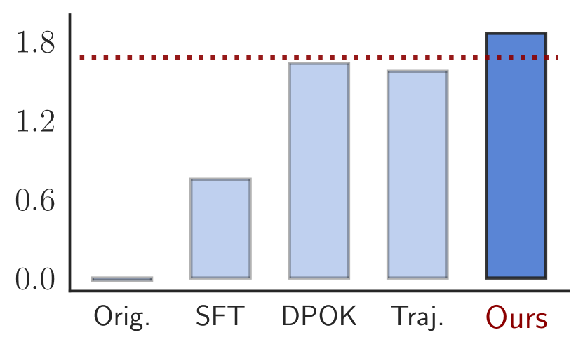
(a) Color

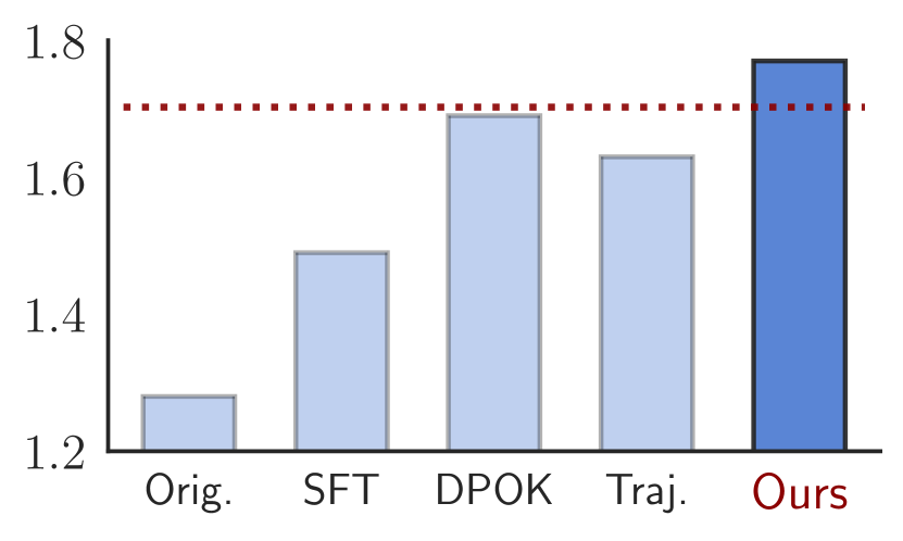
(b) Count

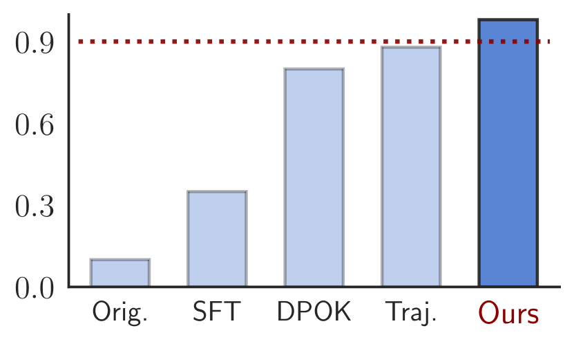
(c) Composition

(d) Location

Figure 1: ImageReward scores for the seen prompts in the single prompt experiments. “Orig.” denotes the original SD1.5. “SFT” is the supervised fine-tuned model. “Traj.” denotes the classical DPO-style objective discussed in Section 2.2, i.e., assuming trajectory-level reward. All our produced results are the average over $100$ image samples. Horizontal line indicates the best baseline result.

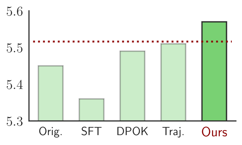
(a) Color

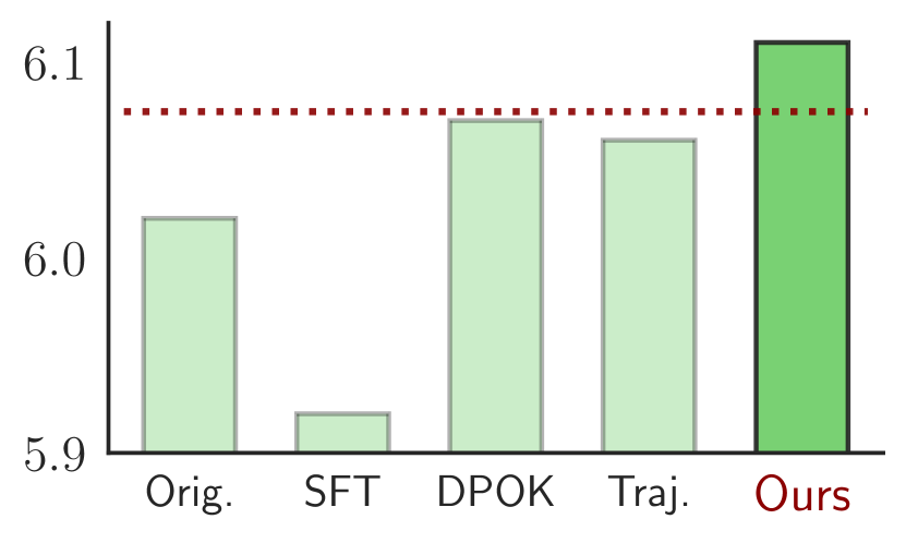
(b) Count

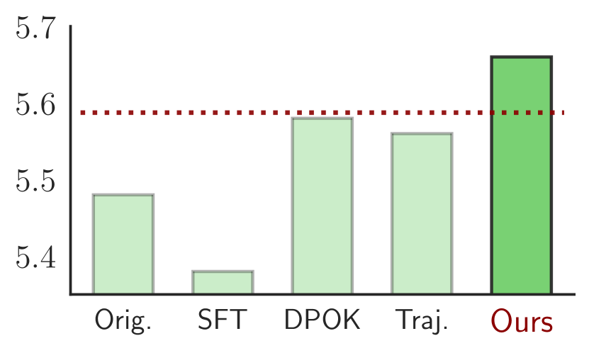
(c) Composition

(d) Location

Figure 2: Aesthetic scores for the seen prompts in the single prompt experiments. Number reporting and abbreviations follow Fig.1.

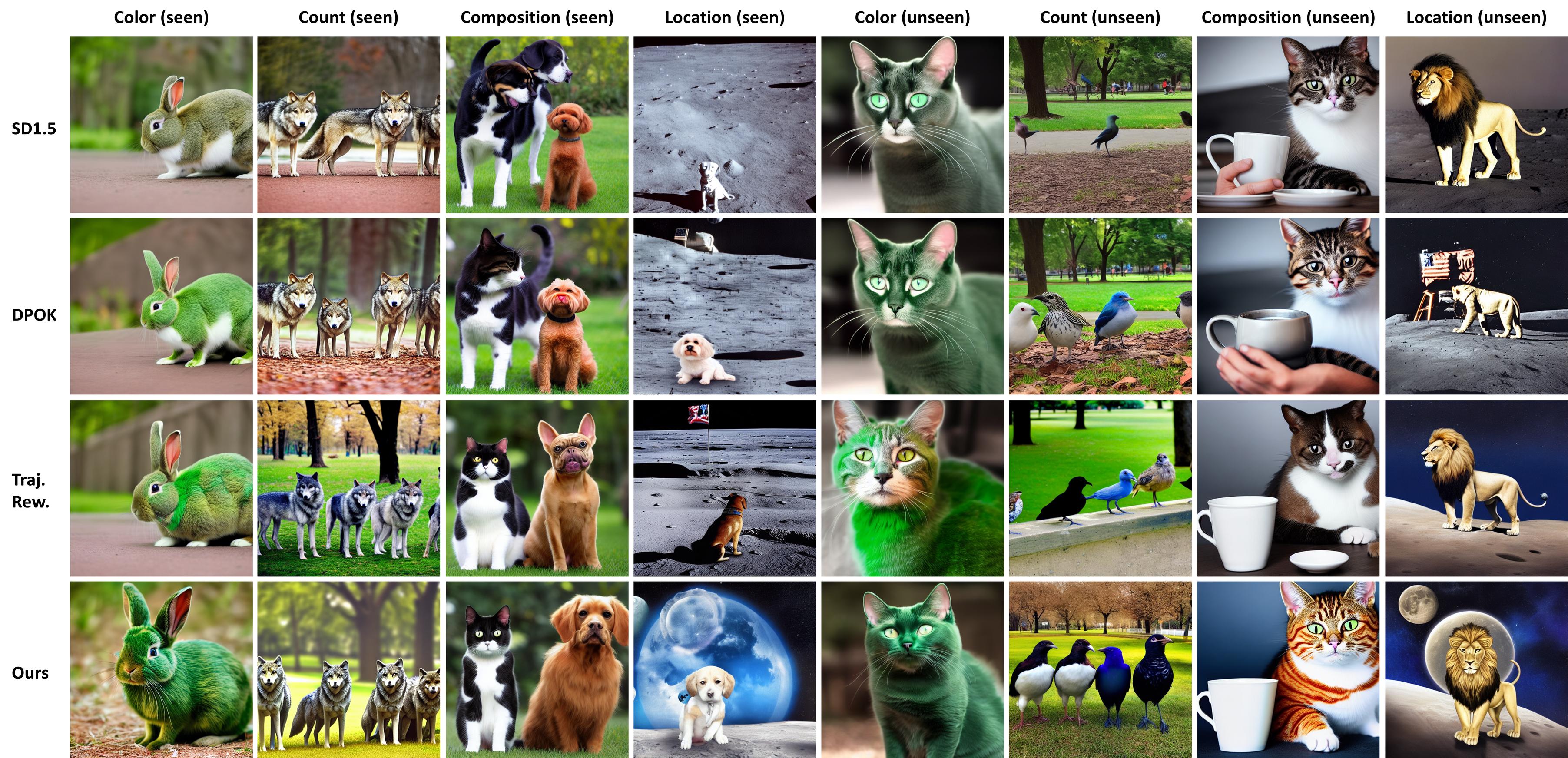
Figure 3: Generated images in the single prompt experiment for both seen and unseen prompts (Table 1). Each comparison is generated from the same random seed. “Traj. Rew.” denotes the classical DPO-style objective of assuming trajectory-level reward (Section 2.2).

Settings.   To facilitate investigation, we first test our method on the single-text-prompt setting in DPOK (Fan et al., 2023), i.e., using one prompt during LoRA fine-tuning. As in DPOK, the goal is to test our method on training the policy T2I to achieve generating objects with specified colors, counts, or locations, or generating composition of two objects. We borrow the seen (training) and unseen prompts from DPOK, which are tabulated in Table 1. In all single prompt experiments, we use the explicit reward model in DPOK, ImageReward (Xu et al., 2023), to generate preference. We report both ImageReward and (Laion) aesthetic score (Schuhmann et al., 2022), averaged over $100$ generated images.

Implementation.   For a fair comparison, we collect the same total amount of $20000$ images/trajectories as DPOK. Rather than its fully-online image-collection strategy, we are motivated by recent RLHF works (e.g., Ziegler et al., 2019; Stiennon et al., 2020; Bai et al., 2022a) to more practically divide our trajectory collection into four stages, where each stage collects $5000$ trajectories and discards the previously collected ones. As in DPOK, we use LoRA with rank $4$ and train the model for a total of $M_{\mathrm{tr}}=10000$ steps, and hence $M_{\mathrm{col}}=2500$ steps, $N_{\mathrm{pr}}=1000$. We set the KL coefficient $C=10$ and $N_{\mathrm{step}}=3$. Section 4.3 (c) ablates the value of $C$. More details on hyperparameters are in Section D.1.

Table 2: HPSv2 and Aesthetic scores for the multiple prompt experiment. Shown here are results for selected relevant and/or strong baselines, with full set of results in Table 4 of Appendix A. The first four result columns are the four styles in HPSv2 test set and “Average” is the overall average. Best result in each metric is bold. Note that HPSv2 paper and repository do not report Aesthetics scores.

Model	Animation	Concept-art	Painting	Photo	Average	Aesthetic
DALL·E 2	27.34	26.54	26.68	27.24	26.95	-
Stable Diffusion v1.5	27.43	26.71	26.73	27.62	27.12	5.62
Stable Diffusion v2.0	27.48	26.89	26.86	27.46	27.17	-
SDXL Refiner 0.9	28.45	27.66	27.67	27.46	27.80	-
Dreamlike Photoreal 2.0	28.24	27.60	27.59	27.99	27.86	-
Trajectory-level Reward	29.37	28.81	28.83	29.16	29.04	5.94
Ours	30.46	29.95	30.01	29.93	30.09	6.31

Results.   We compare our method with the the original SD1.5 (“Orig.”), supervised fine-tuned model (“SFT”), DPOK, and the classical DPO-style objective, i.e., the approach of assuming trajectory-level reward, which is abbreviated as “Traj.”. As discussed in Section 2.2, “Traj.” can be obtained by setting $\gamma=1$ in our loss Eq. (8). We follow the DPOK paper to plot the ImageReward in Fig. 1 and Aesthetic scores in Fig. 2 for the seen prompts, where the results for “Orig.”, “SFT”, and DPOK are directly from the DPOK paper. Fig. 3 shows examples of the generated images from both our method and the baselines. More image comparisons are deferred to Section E.1.

As seen in Fig. 1 and Fig. 2, our method can improve both ImageReward, the preference generating metric, and the unused Aesthetic score. The higher scores of our method over DPOK on both metrics validate the efficacy of our method for T2I’s preference alignment. Comparing with “Traj.”, our method improves more over the original SD1.5, which we attribute to our dense reward perspective, implemented by introducing temporal discounting to emphasize the initial steps of the diffusion reverse chain. From Fig. 3, it is clear that, on both seen and unseen text prompts, our method generates images that are not only faithfully matched with the prompts, but also of higher aesthetic quality, e.g., having more colorful details/backgrounds. Section 4.3 (a) compares the generation trajectories of our method and the baselines. Indeed, our method generates the desired shapes earlier, which helps to explain why it produces better final images.

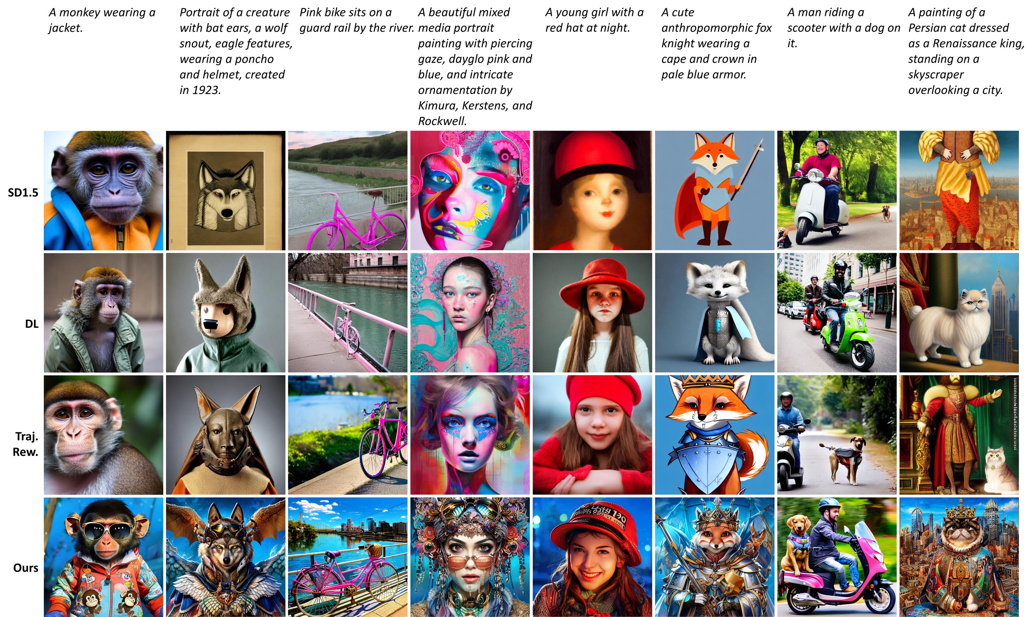
Figure 4: Generated images in the multiple prompt experiments from our method and baselines, with corresponding text prompts on the top. “DL” denotes Dreamlike Photoreal 2.0, the best baseline from the HPSv2 paper. “Traj. Rew.” is the classical DPO-style objective of assuming trajectory-level reward (Section 2.2).

4.2 Multiple Prompts

Settings.   We consider a more challenging setting where we apply our method to train a T2I on the HPSv2 (Wu et al., 2023a) train prompts and evaluate on the HPSv2 test prompts, which have no intersection with the train prompts. We obtain preference by HPSv2 and report the average of both HPSv2 and aesthetic score over all HPSv2 test prompts. Due to the large testset size (3200 prompts), we follow the HPSv2 paper to generate one image per prompt for evaluation.

Implementation.   We use the same trajectory-collection strategy as in the single prompt experiments (Section 4.1). Due to the task complexity and the large size of the HPSv2 train set ($>100000$ prompts), we collect a total of $100,000$ trajectories, divided into ten collection stages. Each stage collects $10000$ trajectories and discards the previously collected ones. We use LoRA with rank $32$ and train the model for a total of $M_{\mathrm{tr}}=40,000$ steps, and hence $M_{\mathrm{col}}=4000$ steps, $N_{\mathrm{pr}}=2000$. We set the KL coefficient $C=12.5$ and ablate the value of $C$ in Section 4.3 (c). We use $N_{\mathrm{step}}=1$ based on compute constraints such as GPU memory. Section D.2 provides more hyperparameter settings.

Results.   Table 2 shows the HPSv2 and Aesthetic scores for our method and selected relevant and/or strong baselines from the HPSv2 paper, with the full set of baseline results deferred to Table 4 of Appendix A. All baselines available in HPSv2 Github Repository are directly cited. As in Section 4.1, we further compare with the classical DPO-style objective of assuming trajectory-level reward (Section 2.2). Fig. 4 shows examples of generated images from our method and baselines, with more image comparisons in Section E.2.

As seen in Table 2, our method is able to improve the preference generating metric, HPSv2, and the unused Aesthetic score. The improvement from our method is larger than the variant of assuming trajectory-level reward, validating our insight of emphasizing the initial part of the T2I generation process, a product of our distinct dense reward perspective. In Fig. 4, we see that our method generates images well matched with the text prompts, in some cases better than the baselines, e.g., on the prompts pertaining to “a girl at night,” “fox knight,” and “scooter with a dog on.” From both short and the more challenging long prompts, our method is able to generate vivid images, often with sophisticated aesthetic shapes. Together with the image examples in Section E.2, Fig. 4 qualitatively validates the efficacy of our method.

4.3 Further Study

This section considers the following four research questions to better understand our method.

(a): Does the T2I from our method indeed generate the desired shapes earlier in the diffusion reverse chain?

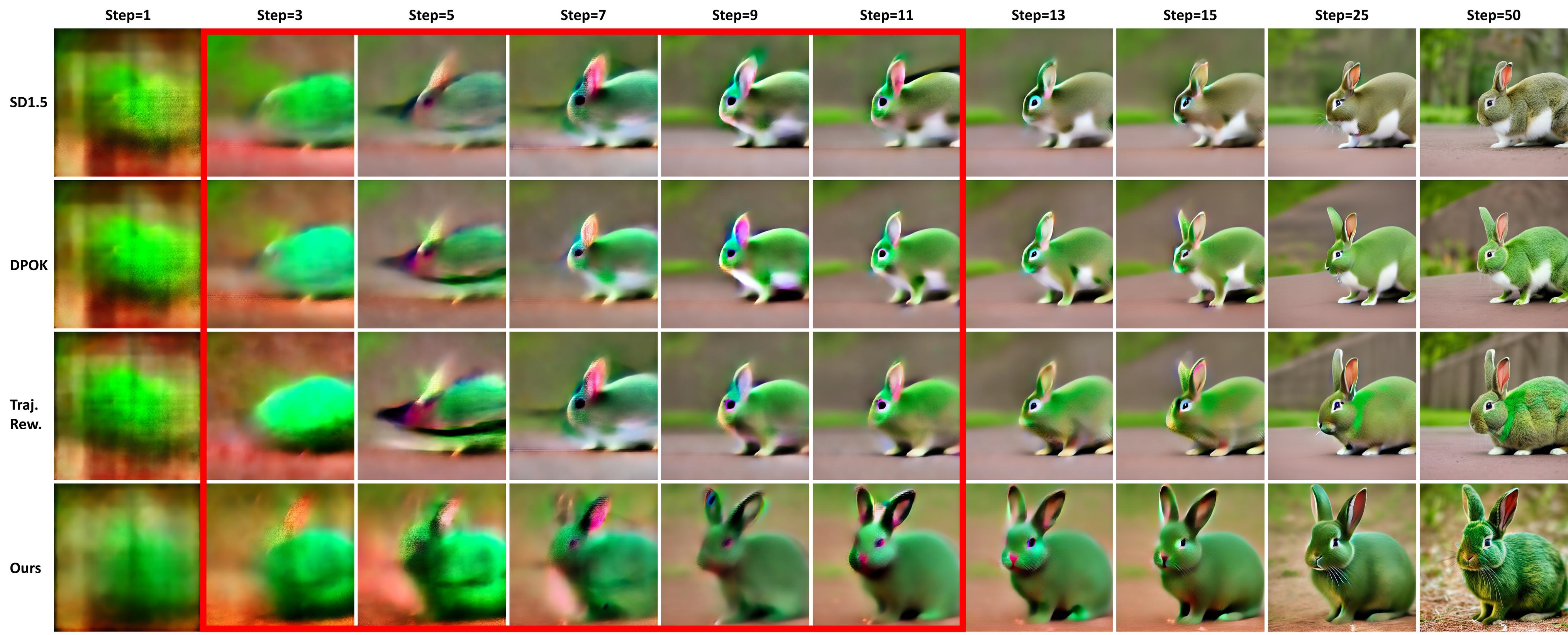
Figure 5: Generation trajectories from our method and the baselines on the prompt “A green colored rabbit.” in the single prompt experiment, correspond to the images in Fig. 3. Shown are the images $\hat{\bm{x}}_{0}$ predicted from the latents at the specified steps of the reverse chain.

As discussed in Section 1, we hypothesize that emphasizing the initial steps of the T2I generation trajectory can help the effectiveness and efficiency of preference alignment. As a verification, Fig. 5 digs into the generated images of the prompt “A green colored rabbit.” in the single prompt experiment, by showing the generation trajectories corresponding to the images in Fig. 3. Specifically, we compare our method and the baselines on the images $\hat{\bm{x}}_{0}$ predicted from the latents at the specified timesteps of the reverse chain. More trajectory comparisions are in Section E.3.

As shown in Fig. 5, and in particular the steps circled out by the red rectangle therein, our method can generate identifiable shapes of a rabbit as early as at Steps $3$ and $5$, while the baselines are still largely unrecognizable, e.g., similar to a mouse. At Step $11$, our method is able to produce a relatively complete image to the given prompt, while the baselines are much cruder. This comparison confirms that, with the incorporation of $\gamma<1$, our method can match the given text prompt earlier in the reverse chain, and thereby more steps later in the chain can be allocated to polish pictorial details and aesthetics, leading to better/preferable final images.

(b): What will happen if we change the value of $\gamma$?

To investigate the impact of temporal discount factor $\gamma$ on training T2I for preference alignment, we consider more values of $\gamma$ between $\gamma=0.9$ used in our main results, and $\gamma=1$ in the classical approach of trajectory-level reward. Fig. 7 plots the preference generating metrics over the training process, under $\gamma\in\{0.9,0.95,0.99,1.0\}$, for single prompt (“A green colored rabbit.”) and multiple prompt experiments. We use the same evaluation protocols as in the main results. For HPSv2, we plot the average over the test set. Patterns on other single prompts are similar.

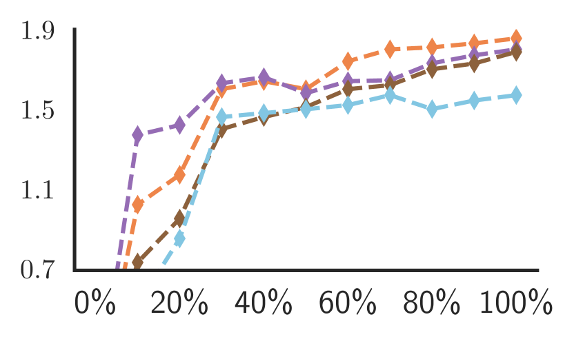
(a) Single (ImageReward)

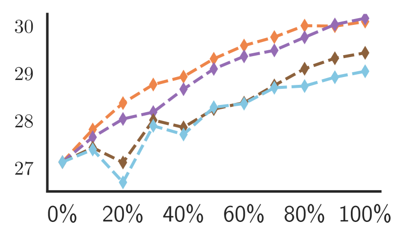
(b) Multiple (HPSv2)

Figure 6: Preference generating metrics over the training process, for the single and multiple prompt experiments under various discount factor $\gamma$. $x$-axis represents $t\%$ of the training process. In (a) all lines start from $-0.02$ at $0\%$, the value of “Orig.” in Fig. 1(a).

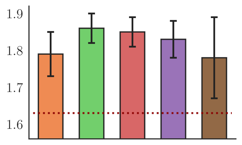
(c) Single (ImageReward)

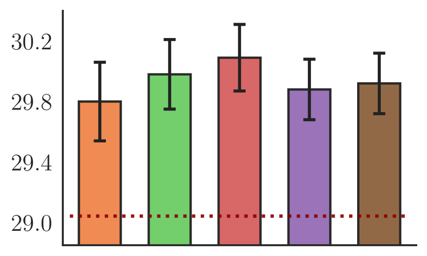
(d) Multiple (HPSv2)

Figure 7: Preference generating metrics with error bars showing one standard deviation, for the single and multiple prompt experiments under various KL coefficient $C$. Horizontal line indicates the best baseline result from Fig. 1(a) and Table 2.

As shown in Fig. 7, using a smaller temporal discount factor, such as $\gamma=0.9$ or $\gamma=0.95$, trains T2I faster and better, compared to larger $\gamma$ values, especially the classical DPO-style loss of $\gamma=1$. Recall from Section 1 that a smaller $\gamma$ emphasizes more on the initial part of the reverse chain, while a sparse trajectory-level reward, equivalent to $\gamma=1$, can incur training instability. In Fig. 7, on both experiments, $\gamma=0.9$ or $\gamma=0.95$ generally leads to a larger improvement at the beginning of the training process. This validates our intuition and prior studies that stressing the earlier steps of the reverse chain could improve the training efficiency of aligning T2I with preference. From Fig. 7, even using $\gamma=0.99$, a small break on the temporal symmetry in the DPO-style losses, can improve training efficiency and stability over the (equivalent) classical setting of $\gamma=1$. This further corroborates the efficacy of our dense reward perspective on T2I’s preference alignment.

(c): Is our method robust to the choice of KL coefficient $C$?

To study the sensitivity of our method to the KL coefficient $C$ in our loss Eq. (8), we vary the value of $C$ from the values set in Sections 4.1 and 4.2. Fig. 7 plots the scores of the preference generating metrics for experiments in the single prompt (“A green colored rabbit.”) and multiple prompts. Other single prompts show similar patterns. For HPSv2, we again plot the average over the test set, with Aesthetic and breakdown scores for each style in Table 5 at Appendix A.

From Fig. 7, we see that our method is generally robust across a range of KL coefficient $C$. A small value of $C$ may be prone to overfitting while a large value may slow down/distract the training process, both of which deteriorate the results.

(d): Are the images from our method indeed preferred by humans?

Table 3: Human evaluation on the multiple prompt experiment. Shown are our “win rate” against the baselines stated in Fig. 4, i.e., the percentage of times our method is preferred in binary comparisons with the specified opponent. A detailed description on the setups is in Section D.3.

Opponent	SD1.5	Dreamlike	Traj. Rew.
Win Rate	$76.8\%$	$68.3\%$	$65.1\%$

To further verify our method, we collect human evaluations on the generated images in the multiple prompt experiment, where binary comparisons between two images from two models are conducted. Table 3 shows the “win rate” of our method over each of the baselines in Fig. 4. Detailed setups of the human evaluation are provided in Section D.3.

The preference for our method over each baseline is evident in Table 3. Recall that the preference source, HPSv2 scorer, is trained on human preference data. The gain of our method over raw SD1.5 verifies the efficacy of our method in aligning T2I with preference. Further, images from our method are more often preferred over the corresponding images from the classical trajectory-level reward objective. This again validates our dense reward perspective that introduces temporal discounting into T2I’s preference alignment.

5 Conclusion

To suit the explicit-reward-free preference-alignment loss to the sequential generation nature of T2I and improve on the classical trajectory-level reward assumption, in this paper, we take on a dense reward perspective and introduce temporal discounting into the alignment objective, motivated by both an easier learning task in RL and the generation hierarchy of the T2I reverse chain. Through experiments and further studies, we validate the efficacy of our method and illustrate its key insight. Future work may involve extending our method to accommodate noisy preference labels and applying our method to broader applications, such as text-to-video or image-to-image generation.

Appendix

Appendix A Tabular Results

Table 4: HPSv2 and Aesthetic scores for the multiple prompt experiment in Section 4.2. The first four result columns are the four styles in the HPSv2 test set and “Average” is the overall average. “Trajectory-level Reward” is the classical DPO-style objective discussed in Section 2.2, which assumes a latent trajectory-level reward function evaluating the entire T2I reverse chain as a whole. All baselines benchmarked in the HPSv2 paper are directly cited from the official Github Repository. Our produced results follow the testing principle in the HPSv2 paper and GitHub Repository. We bold the best result in each metric. Note that HPSv2 paper and Repository do not report the Aesthetics scores.

Model	Animation	Concept-art	Painting	Photo	Average	Aesthetic
GLIDE	23.34	23.08	23.27	24.50	23.55	-
LAFITE	24.63	24.38	24.43	25.81	24.81	-
VQ-Diffusion	24.97	24.70	25.01	25.71	25.10	-
FuseDream	25.26	25.15	25.13	25.57	25.28	-
Latent Diffusion	25.73	25.15	25.25	26.97	25.78	-
DALL·E mini	26.10	25.56	25.56	26.12	25.83	-
VQGAN + CLIP	26.44	26.53	26.47	26.12	26.39	-
CogView2	26.50	26.59	26.33	26.44	26.47	-
Versatile Diffusion	26.59	26.28	26.43	27.05	26.59	-
DALL·E 2	27.34	26.54	26.68	27.24	26.95	-
Stable Diffusion v1.4	27.26	26.61	26.66	27.27	26.95	-
Stable Diffusion v1.5	27.43	26.71	26.73	27.62	27.12	5.62
Stable Diffusion v2.0	27.48	26.89	26.86	27.46	27.17	-
Epic Diffusion	27.57	26.96	27.03	27.49	27.26	-
DeepFloyd-XL	27.64	26.83	26.86	27.75	27.27	-
Openjourney	27.85	27.18	27.25	27.53	27.45	-
MajicMix Realistic	27.88	27.19	27.22	27.64	27.48	-
ChilloutMix	27.92	27.29	27.32	27.61	27.54	-
Deliberate	28.13	27.46	27.45	27.62	27.67	-
SDXL Base 0.9	28.42	27.63	27.60	27.29	27.73	-
Realistic Vision	28.22	27.53	27.56	27.75	27.77	-
SDXL Refiner 0.9	28.45	27.66	27.67	27.46	27.80	-
Dreamlike Photoreal 2.0	28.24	27.60	27.59	27.99	27.86	-
Trajectory-level Reward	29.37	28.81	28.83	29.16	29.04	5.94
Ours	30.46	29.95	30.01	29.93	30.09	6.31

Table 5: HPSv2 and Aesthetic scores for the ablation study on KL coefficient $C$ in Section 4.3 (c). Shown here are breakdown scores of our main method ($\gamma=0.9$) in the multiple prompt experiment under various value of $C$, together with the best baseline in Table 4 of Appendix A. The first four result columns are the four styles in HPSv2 test set and “Average” is the overall average. Within subscript is one standard deviation, as plotted in Fig. 6(d), calculated by the principle described in the HPSv2 paper and GitHub Repository.

Model	HPSv2
	Animation	Concept-art	Painting	Photo	Averaged	Aesthetic
Baseline	29.37	28.81	28.83	29.16	29.04	5.94
$C=7.5$	30.16	29.59	29.64	29.76	29.79 (0.26)	6.24
$C=10.0$	30.36	29.87	29.91	29.80	29.99 (0.23)	6.29
$C=12.5$	30.46	29.95	30.01	29.93	30.09 (0.22)	6.31
$C=15.0$	30.30	29.72	29.74	29.77	29.88 (0.20)	6.23
$C=20.0$	30.28	29.73	29.76	29.95	29.93 (0.20)	6.17

Appendix B Detailed Method Derivation and Proofs

In this section, we provide a detailed step-by-step derivation of our method. For completeness and better readability, some materials in Section 2 will be restated.

B.1 Notation and Assumptions

This section restate the notations and assumptions in Section 2.1 for convenience.

*

We adopt the notation in prior works (e.g., Fan et al., 2023; Black et al., 2023) to formulate the diffusion reverse process under the conditional generation setting as an MDP ${\mathcal{M}}=\left({\mathbb{S}},{\mathbb{A}},{\mathcal{P}},r,\gamma,\rho\right)$. Specifically, let $\pi_{\theta}$ be the T2I with trainable parameters $\theta$, i.e., the policy network; $\left\{{\bm{x}}_{t}\right\}_{t=T}^{0}$ be the diffusion reverse chain of length $T$; and ${\bm{c}}$ be the conditioning variable, i.e., the text conditional in our setting. We have, $\forall\,t$,

$$\begin{array}[]{ccc}s_{t}\triangleq({\bm{x}}_{t},t,{\bm{c}})\,,&{\mathcal{P}}(s_{t+1}\,|\,s_{t},a_{t})\triangleq\delta({\bm{x}}_{t-1},t-1,{\bm{c}})\,,&\pi_{\theta}(a_{t}\,|\,s_{t})\triangleq p_{\theta}({\bm{x}}_{t-1}\,|\,{\bm{x}}_{t},t,{\bm{c}})\,,\\ a_{t}\triangleq{\bm{x}}_{t-1}\,,&\rho(s_{0})\triangleq({\mathcal{N}}({\bm{0}},{\bm{I}}),\delta(T),\delta({\bm{c}}))\,,&r(s_{t},a_{t})\,,\;\gamma\in[0,1]\,,\end{array}$$

where $\delta(\cdot)$ is the delta measure and ${\mathcal{P}}(s_{t+1}\,|\,s_{t},a_{t})$ is a deterministic transition. We denote the reverse chain generated by a (generic) T2I under the text conditional ${\bm{c}}$ as trajectory $\tau$, i.e., $\tau\triangleq(s_{0},a_{0},s_{1},a_{1},\ldots,s_{T})\iff({\bm{x}}_{T},{\bm{x}}_{T-1},\ldots,{\bm{x}}_{0})\,|\,{\bm{c}}$. Note that for notation simplicity, ${\bm{c}}$ is absorbed into the trajectory $\tau$.

Similar to Wallace et al. (2023a), in the method derivation, we consider the setting where we are given two diffusion reverse chains (trajectories) with equal length $T$. For presentation simplicity, assume that $\tau^{1}$ is the better trajectory, i.e., $\tau^{1}\succ\tau^{2}$. Let tuple ${\mathrm{ord}}\triangleq(1,2)$ and $\sigma(\cdot)$ denotes the sigmoid function, i.e., $\sigma(x)=\frac{1}{1+\exp\left(-x\right)}$.

Since in practice the state space of the T2I reverse chain is the continuous embedding space, it is self-evident to assume that any two trajectories do not cross with each other, as follows.

Assumption B.1 (No Crossing Trajectories).

$\forall\,\tau^{i}\neq\tau^{j},s^{i}_{t}\neq s^{j}_{t},\,\forall\,t\in\left\{0,\ldots,T\right\}$.

Furthermore, as in the standard RL setting (Sutton and Barto, 2018), the reward function $r$ in ${\mathcal{M}}$ needs to be bounded, without loss of generality, we assume $r(s,a)\in[0,1]$, and thus $r(s,a)$ may be interpreted as the probability of satisfying the preference when taking action $a$ at state $s$.

*

In RL problems, the performance of a (generic) policy $\pi$ is typically evaluated by the expected cumulative discounted rewards (Sutton and Barto, 2018), which is defined as,

$$\textstyle\eta(\pi)\triangleq\mathbb{E}\left[\sum_{t=0}^{T}\gamma^{t}r(s_{t},a_{t})\,|\,s_{0}\sim\rho(\cdot),a_{t}\sim\pi(\cdot\,|\,s_{t}),s_{t+1}\sim{\mathcal{P}}(\cdot\,|\,s_{t},a_{t}),\forall\,t\geq 0\right]\,.$$ (10)

Note that Eq. (10) above is an extended version of Eq. (1) in Section 2.1.

*

Remark 2.1 in Section 2.1 discusses the practical rationality of $e(\tau)$ in T2I’s preference alignment.

B.2 Step-by-step Derivation of Our Method

B.2.1 Expression of $e(\tau)$

We can express $\eta(\pi)$ in Eq. (10) by the (discounted) stationary distribution $d_{\pi}(s)$ of the policy $\pi$, defined as $d_{\pi}(s)\propto\sum_{t=0}^{T}\gamma^{t}\Pr(s_{t}=s\,|\,\pi,{\mathcal{P}})$, up to the (positive) normalizing constant. We have

$$\begin{split}\eta(\pi)&=\mathbb{E}_{a_{t}\sim\pi,s_{t+1}\sim{\mathcal{P}}}\left[\sum_{t=0}^{T}\gamma^{t}r(s_{t},a_{t})\right]=\sum_{t=0}^{T}\int_{\mathbb{S}}\Pr(s_{t}=s\,|\,\pi,{\mathcal{P}})\int_{{\mathbb{A}}}\pi(a\,|\,s)\,\gamma^{t}\,r(s,a)\mathop{}\!\mathrm{d}a\mathop{}\!\mathrm{d}s\\ &=\int_{\mathbb{S}}\sum_{t=0}^{T}\gamma^{t}\Pr(s_{t}=s\,|\,\pi,{\mathcal{P}})\int_{{\mathbb{A}}}\pi(a\,|\,s)\,r(s,a)\mathop{}\!\mathrm{d}a\mathop{}\!\mathrm{d}s\\ &\propto\int_{\mathbb{S}}d_{\pi}(s)\int_{{\mathbb{A}}}\pi(a\,|\,s)\,r(s,a)\mathop{}\!\mathrm{d}a\mathop{}\!\mathrm{d}s=\mathbb{E}_{s\sim d_{\pi}(s)}\mathbb{E}_{a\sim\pi(a\,|\,s)}\left[r(s,a)\right]\,.\end{split}$$

The goal of RL is to maximize the expected cumulative discounted rewards $\eta(\pi)$, which is unfortunately difficult due to the complicate relationship between $d_{\pi}(s)$ and $\pi$. We therefore optimize an off-policy approximation of $\eta(\pi)$ by employing an approximate objective common in prior RL works (e.g., Kakade and Langford, 2002; Peters et al., 2010; Schulman et al., 2015; Abdolmaleki et al., 2018; Peng et al., 2019; Yang et al., 2022b, a). Specifically, we change $d_{\pi}(s)$ to $d_{\pi_{O}}(s)$ for some “old” policy $\pi_{O}$, from which we generate the off-policy trajectories/data. We further add a KL regularization on $\pi$ towards the initial pre-trained T2I $\pi_{I}$ to avoid generating unnatural images. With these, we arrive at the following constrained policy search problem

$$\begin{split}\arg\max_{\pi}\quad&\mathbb{E}_{s\sim d_{\pi_{O}}(s)}\mathbb{E}_{a\sim\pi(a\,|\,s)}\left[r(s,a)\right]\\ \mathrm{s.t.}\quad&D_{\mathrm{KL}}\left(\pi(\cdot\,|\,s)\,\|\,\pi_{I}(\cdot\,|\,s)\right)\leq\epsilon\,,\quad\forall\,s\in{\mathbb{S}}\\ &\int_{\mathbb{A}}\pi(a\,|\,s)\mathop{}\!\mathrm{d}a=1,\quad\forall\,s\in{\mathbb{S}},\end{split}$$ (11)

where $\pi_{O}$ may be chosen as $\pi_{I}$ or some saved policy checkpoint not far away from $\pi_{I}$.

Enforcing the pointwise KL-regularization in Eq. (11) is difficult, as in AWR (Peng et al., 2019), we change the pointwise KL-regularization into enforcing the regularization only in expectation $\mathbb{E}_{s\sim d_{\pi_{O}}}\left[\cdots\right]$ and change Eq. (11) into a penalized maximization problem

$$\begin{split}\arg\max_{\pi}\quad&\mathbb{E}_{s\sim d_{\pi_{O}}(s)}\mathbb{E}_{a\sim\pi(a\,|\,s)}\left[r(s,a)\right]-C\cdot\mathbb{E}_{s\sim d_{\pi_{O}}(s)}\left[D_{\mathrm{KL}}\left(\pi(\cdot\,|\,s)\,\|\,\pi_{I}(\cdot\,|\,s)\right)\right]\\ \mathrm{s.t.}\quad&\int_{\mathbb{A}}\pi(a\,|\,s)\mathop{}\!\mathrm{d}a=1,\quad\forall\,s\in{\mathbb{S}}.\end{split}$$ (12)

The Lagrange form of the maximization problem Eq. (12) is

$\forall\,s\in{\mathbb{S}},a\in{\mathbb{A}}$, the optimal policy under ${\mathcal{L}}(\pi)$ can be obtained by setting the derivation w.r.t. $\pi(a\,|\,s)$ equal to $0$. We have

where $\pi^{*}$ is the optimal (regularized) policy under $r$. We ignore the word “regularized” hereafter to avoid wordiness.

From Eq. (14), we can also get the formula for the optimal policy $\pi^{*}$ as

where $Z(s)$ denotes the partition function, taking the form

$$Z(s)=\int_{\mathbb{A}}\exp\left(\frac{1}{C}r(s,a)\right)\pi_{I}(a\,|\,s)\mathop{}\!\mathrm{d}a.$$

For a given trajectory $\tau=(s_{0},a_{0},s_{1},a_{1},\ldots,s_{T})$, the quality evaluation $e(\tau)$ can be expressed by $\pi^{*}$ as

$$\begin{split}e(\tau)&\triangleq\sum_{t=0}^{T}\gamma^{t}r(s_{t},a_{t})=C\sum_{t=0}^{T}\gamma^{t}\log\frac{\pi^{*}(a_{t}\,|\,s_{t})}{\pi_{I}(a_{t}\,|\,s_{t})}+C\sum_{t=0}^{T}\gamma^{t}\left(1+\frac{\alpha_{s_{t}}}{Cd_{\pi_{O}}(s_{t})}\right)\\ &=C\sum_{t=0}^{T}\gamma^{t}\log\frac{\pi^{*}(a_{t}\,|\,s_{t})}{\pi_{I}(a_{t}\,|\,s_{t})}+C\sum_{t=0}^{T}\gamma^{t}\log Z(s_{t}).\end{split}$$ (16)

Since the trajectory $\tau$ and hence all $s_{t}$’s are given, $Z(s_{t})$’s are constant and the summation over $\log Z(s_{t})$ is a “property” of the trajectory $\tau$, we thus denote $\log Z(\tau)\triangleq\sum_{t=0}^{T}\gamma^{t}\log Z(s_{t})$ for notation simplicity. Then the formula for $e(\tau)$ becomes

$$e(\tau)=C\sum_{t=0}^{T}\left[\gamma^{t}\log\frac{\pi^{*}(a_{t}\,|\,s_{t})}{\pi_{I}(a_{t}\,|\,s_{t})}\right]+C\log Z(\tau)\,.$$ (17)

B.2.2 Loss Function for T2I/Policy Training

Recall that we are given two diffusion reverse chains (trajectories) $\left\{\tau^{1},\tau^{2}\right\}$ with equal length $T$. Also recall the notation that $\tau^{1}$ is the better trajectory, i.e., $\tau^{1}\succ\tau^{2}$, the tuple ${\mathrm{ord}}\triangleq(1,2)$ and $\sigma(\cdot)$ denotes the sigmoid function. Under the Bradley-Terry model of pairwise preference, the probability of ${\mathrm{ord}}$ under $\left\{e\left(\tau^{k}\right)\right\}_{k=1}^{2}$ and hence $\pi^{*}$ is

$$\Pr\left({\mathrm{ord}}\,|\,\pi^{*},\left\{e\left(\tau^{k}\right)\right\}_{k=1}^{2}\right)=\frac{\exp\left(e\left(\tau^{1}\right)\right)}{\exp\left(e\left(\tau^{1}\right)\right)+\exp\left(e\left(\tau^{2}\right)\right)}=\sigma\left(e\left(\tau^{1}\right)-e\left(\tau^{2}\right)\right)\,,$$ (18)

where we explicitly put $\pi^{*}$ into the condition variables for better readability.

From Eq. (17), $e\left(\tau^{1}\right)$ and $e\left(\tau^{2}\right)$ respectively contains the “partition functions” $Z(\tau^{1})$ and $Z(\tau^{2})$, both of which are intractable. We argue that $Z(\tau^{1})\geq Z(\tau^{2})$, which will be critical for providing a tractable lower bound of Eq. (18) that cancels out these partition functions. Our argument is based on the reward-shaping technique (Ng et al., 1999), as follows.

*

*

Remark B.2.

The only difference between the MDPs ${\mathcal{M}}$ and ${\mathcal{M}}^{\prime}$ is the reward function ($r$ v.s. $r^{\prime}$). In particular, they share the same state and action space. Therefore, it make sense to consider the invariance of the optimal policy in these two MDPs. Basically, in these two MDPs, at each state, the optimal policies take the same action with the same probability.

Proof of Section 2.2.

Denote the optimal policy under the MDP ${\mathcal{M}}^{\prime}$ as $\pi^{*^{\prime}}$, we have

$$\pi^{*^{\prime}}(a\,|\,s) =\frac{\exp\left(\frac{1}{C}\left(r(s,a)+\Phi(s)\right)\right)\pi_{I}(a\,|\,s)}{\int_{\mathbb{A}}\exp\left(\frac{1}{C}\left(r(s,a)+\Phi(s)\right)\right)\pi_{I}(a\,|\,s)\mathop{}\!\mathrm{d}a}$$ (19)

$$=\frac{\exp\left(\frac{1}{C}\Phi(s)\right)\exp\left(\frac{1}{C}r(s,a)\right)\pi_{I}(a\,|\,s)}{\exp\left(\frac{1}{C}\Phi(s)\right)\int_{\mathbb{A}}\exp\left(\frac{1}{C}r(s,a)\right)\pi_{I}(a\,|\,s)\mathop{}\!\mathrm{d}a}$$

$$=\pi^{*}(a\,|\,s),$$

since $\exp\left(\frac{1}{C}\Phi(s)\right)$ is independent of the integration dummy-variable $a$ in the denominator. ∎

* *

With the reshaping technique, we can justify our previous argument that $Z(\tau^{1})\geq Z(\tau^{2})$ as follows.

*

We defer the proof of Theorem 2.2 to Section B.3.

*

*

With Theorem 2.2, we can lower bound $\Pr\left({\mathrm{ord}}\,|\,\pi^{*},\left\{e\left(\tau^{k}\right)\right\}_{k=1}^{2}\right)$ in Eq. (18) by a simpler formula. After plugging in the expression of $e(\tau)$ w.r.t. the optimal policy $\pi^{*}$ in Eq. (17), we have,

$$\begin{split}\Pr\left({\mathrm{ord}}\,|\,\pi^{*},\left\{e\left(\tau^{k}\right)\right\}_{k=1}^{2}\right)&=\frac{\exp\left(C\sum_{t=0}^{T}\gamma^{t}\log\frac{\pi^{*}\left(a^{1}_{t}\,|\,s^{1}_{t}\right)}{\pi_{I}\left(a^{1}_{t}\,|\,s^{1}_{t}\right)}\right)Z\left(\tau^{1}\right)^{C}}{\sum_{i=1}^{2}\exp\left(C\sum_{t=0}^{T}\gamma^{t}\log\frac{\pi^{*}\left(a^{i}_{t}\,|\,s^{i}_{t}\right)}{\pi_{I}\left(a^{i}_{t}\,|\,s^{i}_{t}\right)}\right)Z\left(\tau^{i}\right)^{C}}\\ &\geq\frac{\exp\left(C\sum_{t=0}^{T}\gamma^{t}\log\frac{\pi^{*}\left(a^{1}_{t}\,|\,s^{1}_{t}\right)}{\pi_{I}\left(a^{1}_{t}\,|\,s^{1}_{t}\right)}\right)Z\left(\tau^{1}\right)^{C}}{\sum_{i=1}^{2}\exp\left(C\sum_{t=0}^{T}\gamma^{t}\log\frac{\pi^{*}\left(a^{i}_{t}\,|\,s^{i}_{t}\right)}{\pi_{I}\left(a^{i}_{t}\,|\,s^{i}_{t}\right)}\right)Z\left(\tau^{1}\right)^{C}}\\ &=\frac{\exp\left(C\sum_{t=0}^{T}\gamma^{t}\log\frac{\pi^{*}\left(a^{1}_{t}\,|\,s^{1}_{t}\right)}{\pi_{I}\left(a^{1}_{t}\,|\,s^{1}_{t}\right)}\right)}{\sum_{i=1}^{2}\exp\left(C\sum_{t=0}^{T}\gamma^{t}\log\frac{\pi^{*}\left(a^{i}_{t}\,|\,s^{i}_{t}\right)}{\pi_{I}\left(a^{i}_{t}\,|\,s^{i}_{t}\right)}\right)}\;.\end{split}$$ (20)

By our definition of the quality evaluation $e(\tau)$, a better trajectory $\tau$ comes with a higher $e(\tau)$. Hence $\exp\left(e\left(\tau^{1}\right)\right)/\left(\sum_{i=1}^{2}\exp\left(e\left(\tau^{i}\right)\right)\right)\geq\exp\left(e\left(\tau^{2}\right)\right)/\left(\sum_{i=1}^{2}\exp\left(e\left(\tau^{i}\right)\right)\right)$. In other words, among $\left\{\tau^{1},\tau^{2}\right\}$, $\tau^{1}$ should have the highest chance to be ranked top under the Bradley-Terry preference model Eq. (18) induced by the true reward $r(s,a)$. Thus we conclude that $\Pr\left({\mathrm{ord}}\,|\,\pi^{*},\left\{e\left(\tau^{k}\right)\right\}_{k=1}^{2}\right)=\max\Pr\left(\cdot\,|\,\pi^{*},\left\{e\left(\tau^{k}\right)\right\}_{k=1}^{2}\right)$, i.e., in the MDP ${\mathcal{M}}$ (or ${\mathcal{M}}^{\prime}$) with additional components $(\pi_{I},C)$ and conditioning on $\pi^{*}$, ${\mathrm{ord}}$ should be the most probable ordering under the Bradley-Terry model Eq. (18). Thus, in order to approximate $\pi^{*}$, our parametrized policy $\pi_{\theta}$ ought to maximize the likelihood of ${\mathrm{ord}}$ under the corresponding Bradley-Terry model constructed by changing $\pi^{*}$ to $\pi_{\theta}$. Based on this intuition, we train $\pi_{\theta}$ by maximizing the lower bound of the Bradley-Terry likelihood of ${\mathrm{ord}}$ in Eq. (20), which leads to the negative-log-likelihood loss for an minimization objective for training $\pi_{\theta}$ as

$${\mathcal{L}}_{\gamma}\left(\theta\,|\,{\mathrm{ord}},\left\{e\left(\tau^{k}\right)\right\}_{k=1}^{2}\right)= -\log\sigma\left(C\sum_{t=0}^{T}\gamma^{t}\left[\log\frac{\pi_{\theta}\left(a^{1}_{t}\,|\,s^{1}_{t}\right)}{\pi_{I}\left(a^{1}_{t}\,|\,s^{1}_{t}\right)}-\log\frac{\pi_{\theta}\left(a^{2}_{t}\,|\,s^{2}_{t}\right)}{\pi_{I}\left(a^{2}_{t}\,|\,s^{2}_{t}\right)}\right]\right)$$ (21)

$$= -\log\sigma\left(C\mathbb{E}_{t\sim\mathrm{Cat}\left(\left\{\gamma^{t}\right\}\right)}\left[\log\frac{\pi_{\theta}\left(a^{1}_{t}\,|\,s^{1}_{t}\right)}{\pi_{I}\left(a^{1}_{t}\,|\,s^{1}_{t}\right)}-\log\frac{\pi_{\theta}\left(a^{2}_{t}\,|\,s^{2}_{t}\right)}{\pi_{I}\left(a^{2}_{t}\,|\,s^{2}_{t}\right)}\right]\right)$$

where $\mathrm{Cat}\left(\left\{\gamma^{t}\right\}\right)$ denotes the categorical distribution on $\left\{0,\ldots,T\right\}$ with the probability vector $\{\gamma^{t}/\sum_{t^{\prime}}\gamma^{t^{\prime}}\}_{t=0}^{T}$ and $C$ is overloaded to absorb the normalization constant.

B.3 Proofs

B.3.1 Derivation of the Gradient in Eq. (9)

In this section we derive the gradient of ${\mathcal{L}}_{\gamma}\left(\theta\,|\,{\mathrm{ord}},\left\{e\left(\tau^{k}\right)\right\}_{k=1}^{2}\right)$ in Eq. (21) with respect to $\theta$, which shows up in Section 2.2.

Since Eq. (21) is an objective for a minimization problem, the gradient update direction is $-\nabla_{\theta}{\mathcal{L}}_{\gamma}\left(\theta\,|\,{\mathrm{ord}},\left\{e\left(\tau^{k}\right)\right\}_{k=1}^{2}\right)=\nabla_{\theta}\left(-{\mathcal{L}}_{\gamma}\left(\theta\,|\,{\mathrm{ord}},\left\{e\left(\tau^{k}\right)\right\}_{k=1}^{2}\right)\right)$. The gradient can be derived by chain rule as follows. For notation simplicity, we denote $\widetilde{e}(\tau^{k})\triangleq C\sum_{t=0}^{T}\gamma^{t}\log\frac{\pi_{\theta}\left(a^{k}_{t}\,|\,s^{k}_{t}\right)}{\pi_{I}\left(a^{k}_{t}\,|\,s^{k}_{t}\right)}$. We have

$$\begin{split}-{\mathcal{L}}_{\gamma}\left(\theta\,|\,{\mathrm{ord}},\left\{e\left(\tau^{k}\right)\right\}_{k=1}^{2}\right)&=-\log\left(1+\exp\left(\widetilde{e}\left(\tau^{2}\right)-\widetilde{e}\left(\tau^{1}\right)\right)\right)\end{split}$$

$$\begin{split}\frac{\partial\left(-{\mathcal{L}}_{\gamma}\left(\theta\,|\,{\mathrm{ord}},\left\{e\left(\tau^{k}\right)\right\}_{k=1}^{2}\right)\right)}{\partial\left(\widetilde{e}\left(\tau^{2}\right)-\widetilde{e}\left(\tau^{1}\right)\right)}&=-\frac{\exp\left(\widetilde{e}\left(\tau^{2}\right)\right)}{\exp\left(\widetilde{e}\left(\tau^{1}\right)\right)+\exp\left(\widetilde{e}\left(\tau^{2}\right)\right)}\end{split}$$

$$\forall\,k=1,2,\quad\frac{\partial\widetilde{e}\left(\tau^{k}\right)}{\partial\theta} =C\sum_{t=0}^{T}\gamma^{t}\nabla_{\theta}\log\frac{\pi_{\theta}\left(a^{k}_{t}\,|\,s^{k}_{t}\right)}{\pi_{I}\left(a^{k}_{t}\,|\,s^{k}_{t}\right)}=C\sum_{t=0}^{T}\gamma^{t}\frac{\pi_{I}\left(a^{k}_{t}\,|\,s^{k}_{t}\right)}{\pi_{\theta}\left(a^{k}_{t}\,|\,s^{k}_{t}\right)}\nabla_{\theta}\pi_{\theta}\left(a^{k}_{t}\,|\,s^{k}_{t}\right)$$

$$=C\sum_{t=0}^{T}\gamma^{t}\pi_{I}\left(a^{k}_{t}\,|\,s^{k}_{t}\right)\nabla_{\theta}\log\pi_{\theta}\left(a^{k}_{t}\,|\,s^{k}_{t}\right)$$

$$\frac{\partial\left(-{\mathcal{L}}_{\gamma}\left(\theta\,|\,{\mathrm{ord}},\left\{e\left(\tau^{k}\right)\right\}_{k=1}^{2}\right)\right)}{\partial\theta} =\frac{\partial\left(-{\mathcal{L}}_{\gamma}\left(\theta\,|\,{\mathrm{ord}},\left\{e\left(\tau^{k}\right)\right\}_{k=1}^{2}\right)\right)}{\partial\left(\widetilde{e}\left(\tau^{2}\right)-\widetilde{e}\left(\tau^{1}\right)\right)}\left(\frac{\partial\widetilde{e}\left(\tau^{2}\right)}{\partial\theta}-\frac{\partial\widetilde{e}\left(\tau^{1}\right)}{\partial\theta}\right)$$

$$=-\frac{\exp\left(\widetilde{e}\left(\tau^{2}\right)\right)}{\exp\left(\widetilde{e}\left(\tau^{1}\right)\right)+\exp\left(\widetilde{e}\left(\tau^{2}\right)\right)}\left(\frac{\partial\widetilde{e}\left(\tau^{2}\right)}{\partial\theta}-\frac{\partial\widetilde{e}\left(\tau^{1}\right)}{\partial\theta}\right)$$

$$=\frac{\exp\left(\widetilde{e}\left(\tau^{2}\right)\right)}{\exp\left(\widetilde{e}\left(\tau^{1}\right)\right)+\exp\left(\widetilde{e}\left(\tau^{2}\right)\right)}\left(\frac{\partial\widetilde{e}\left(\tau^{1}\right)}{\partial\theta}-\frac{\partial\widetilde{e}\left(\tau^{2}\right)}{\partial\theta}\right)$$

$$=\frac{\exp\left(\widetilde{e}\left(\tau^{2}\right)-\widetilde{e}\left(\tau^{1}\right)\right)}{1+\exp\left(\widetilde{e}\left(\tau^{2}\right)-\widetilde{e}\left(\tau^{1}\right)\right)}\times C\times\sum_{t=0}^{T}\gamma^{t}\bigg{(}\pi_{I}\left(a^{1}_{t}\,|\,s^{1}_{t}\right)\nabla_{\theta}\log\pi_{\theta}\left(a^{1}_{t}\,|\,s^{1}_{t}\right)$$

$$\qquad\qquad\qquad\qquad\qquad\qquad\qquad\qquad\qquad-\pi_{I}\left(a^{2}_{t}\,|\,s^{2}_{t}\right)\nabla_{\theta}\log\pi_{\theta}\left(a^{2}_{t}\,|\,s^{2}_{t}\right)\bigg{)}.$$

B.3.2 Proof of Theorem 2.2

As a reminder, in Section 2.2 we consider a more general case where we are given a finite number $K$ of trajectories whose preference ordering is assume to be $\tau^{1}\succ\tau^{2}\succ\cdots\succ\tau^{K}$. Each trajectory $\tau^{k}$ takes the form $\tau^{k}=(s^{k}_{0},a^{k}_{0},s^{k}_{1},a^{k}_{1},\ldots,s^{k}_{T})$.

A Simplified Case without Reward Shaping.  

To gain some intuitions, we first present a simplified setting where the distribution $\pi_{I}$ is deterministic on the given samples, i.e., $\pi_{I}\left(a^{i}_{t}\,|\,s^{i}_{t}\right)=\delta\left(a^{i}_{t}\,|\,s^{i}_{t}\right)$. In this scenario, Theorem 2.2 can be proved without using the reward-shaping argument.

We now state and proof this special case of Theorem 2.2.

Theorem B.3 (A special case of Theorem 2.2).

If the initial distribution $\pi_{I}\left(a^{i}_{t}\,|\,s^{i}_{t}\right)=\delta\left(a^{i}_{t}\,|\,s^{i}_{t}\right)$, then the original reward function $r(s,a)$ satisfies $Z(\tau^{1})\geq Z(\tau^{2})\geq\cdots\geq Z(\tau^{K})$.

Proof.

Our target is $\forall\,k\in\left\{1,\ldots,K\right\},i\in\left\{k,\ldots,K\right\}$,

$$\begin{split}Z(\tau^{k})\geq Z(\tau^{i})&\iff\log Z(\tau^{k})\geq\log Z(\tau^{i})\iff\sum_{t=0}^{T}\gamma^{t}\log Z\left(s^{k}_{t}\right)\geq\sum_{t=0}^{T}\gamma^{t}\log Z\left(s^{i}_{t}\right)\\ &\iff\sum_{t=0}^{T}\gamma^{t}\left(\log Z\left(s^{k}_{t}\right)-\log Z\left(s^{i}_{t}\right)\right)\geq 0.\end{split}$$

In the special case of $\pi_{I}\left(a^{i}_{t}\,|\,s^{i}_{t}\right)=\delta\left(a^{i}_{t}\,|\,s^{i}_{t}\right)$, with the original reward function $r(s,a)$, we have

$$\begin{split}Z\left(s^{i}_{t}\right)=\int_{\mathbb{A}}\exp\left(\frac{1}{C}r\left(s^{i}_{t},a\right)\right)\pi_{I}\left(a\,|\,s^{i}_{t}\right)\mathop{}\!\mathrm{d}a&=\exp\left(\frac{1}{C}r\left(s^{i}_{t},a^{i}_{t}\right)\right)\implies\log Z\left(s^{i}_{t}\right)=\frac{1}{C}r\left(s^{i}_{t},a^{i}_{t}\right)\\ \implies\log Z\left(s^{k}_{t}\right)-\log Z\left(s^{i}_{t}\right)&=\frac{1}{C}\left(r\left(s^{k}_{t},a^{k}_{t}\right)-r\left(s^{i}_{t},a^{i}_{t}\right)\right)\\ \implies\sum_{t=0}^{T}\gamma^{t}\left(\log Z\left(s^{k}_{t}\right)-\log Z\left(s^{i}_{t}\right)\right)&=\frac{1}{C}\sum_{t=0}^{T}\gamma^{t}\left(r\left(s^{k}_{t},a^{k}_{t}\right)-r\left(s^{i}_{t},a^{i}_{t}\right)\right)\,.\end{split}$$

Since $\tau^{k}\succ\tau^{i}\iff e\left(\tau^{k}\right)>e\left(\tau^{i}\right)$, plugging in the definition of $e\left(\tau\right)$, we get,

$$e\left(\tau^{k}\right)>e\left(\tau^{i}\right)\iff\sum_{t=0}^{T}\gamma^{t}r(s^{k}_{t},a^{k}_{t})\geq\sum_{t=0}^{T}\gamma^{t}r(s^{i}_{t},a^{i}_{t}) \iff\sum_{t=0}^{T}\gamma^{t}\left(r(s^{k}_{t},a^{k}_{t})-r(s^{i}_{t},a^{i}_{t})\right)\geq 0\iff$$

$$\sum_{t=0}^{T}\gamma^{t}\log Z\left(s^{k}_{t}\right)\geq\sum_{t=0}^{T}\gamma^{t}\log Z\left(s^{i}_{t}\right) \iff\log Z\left(\tau^{k}\right)\geq\log Z\left(\tau^{i}\right)\iff Z\left(\tau^{k}\right)\geq Z\left(\tau^{i}\right)\,.$$

Hence the original reward function $r(s,a)$, without shaping, satisfies the ordering $Z\left(\tau^{k}\right)\geq Z\left(\tau^{i}\right)$. Notice that all the above steps are “$\iff$” and recall our assumption that $\tau^{1}\succ\tau^{2}\succ\cdots\succ\tau^{K}\implies\tau^{k}\succ\tau^{i}\iff k\geq i$. It is clear that such an ordering is transitive, in a sense that, if $\tau^{k}\succ\tau^{i}\succ\tau^{j}$, then

$$\left.\begin{aligned} \tau^{k}\succ\tau^{i}\implies k\geq i\\ \tau^{i}\succ\tau^{j}\implies i\geq j\\ \end{aligned}\right\}\implies k\geq j\implies Z\left(\tau^{k}\right)\geq Z\left(\tau^{j}\right)\,.$$

Since $k$ is arbitrary, we conclude that $Z(\tau^{1})\geq Z(\tau^{2})\geq\cdots\geq Z(\tau^{K})$, as desired. ∎

The General Case  

We restate Theorem 2.2 here for better readability.

*

As discussed in Remark 2.2, for the value of $C$, we technically requires that $\forall(s,a)\in{\mathbb{S}}\times{\mathbb{A}},r(s,a)/C\leq\mathrm{const}\approx 1.79$. Hence, under Assumption 2.1, $C\geq 0.56$ will suffice. This constraint provides some information on the setting of hyperparameter $C$.

Proof.

Under the shaped reward $r^{\prime}(s,a)=r(s,a)+\Phi(s)$, $Z\left(s^{k}_{t}\right)$ takes the form

$$\begin{split}Z\left(s^{k}_{t}\right)&=\int_{\mathbb{A}}\exp\left(\frac{1}{C}r\left(s^{k}_{t},a\right)+\frac{1}{C}\Phi\left(s^{k}_{t}\right)\right)\pi_{I}\left(a\,|\,s^{k}_{t}\right)\mathop{}\!\mathrm{d}a\\ &=\exp\left(\frac{1}{C}\Phi\left(s^{k}_{t}\right)\right)\int_{\mathbb{A}}\exp\left(\frac{1}{C}r\left(s^{k}_{t},a\right)\right)\pi_{I}\left(a\,|\,s^{k}_{t}\right)\mathop{}\!\mathrm{d}a\\ &=\exp\left(\frac{1}{C}\Phi\left(s^{k}_{t}\right)\right)\mathbb{E}_{a\sim\pi_{I}\left(\cdot\,|\,s^{k}_{t}\right)}\left[\exp\left(\frac{1}{C}r\left(s^{k}_{t},a\right)\right)\right].\end{split}$$

Taking $\log$, by Jensen’s inequality, we have

$$\log Z\left(s^{k}_{t}\right) =\frac{1}{C}\Phi\left(s^{k}_{t}\right)+\log\mathbb{E}_{a\sim\pi_{I}\left(\cdot\,|\,s^{k}_{t}\right)}\left[\exp\left(\frac{1}{C}r\left(s^{k}_{t},a\right)\right)\right]\geq\frac{1}{C}\Phi\left(s^{k}_{t}\right)+\mathbb{E}_{a\sim\pi_{I}\left(\cdot\,|\,s^{k}_{t}\right)}\left[\frac{1}{C}r\left(s^{k}_{t},a\right)\right].$$

On the other hand, we also have

Taking $\log$, we have

$$\begin{split}\log Z\left(s^{i}_{t}\right)&=\frac{1}{C}\Phi\left(s^{i}_{t}\right)+\log\left(\mathbb{E}_{a\sim\pi_{I}\left(\cdot\,|\,s^{i}_{t}\right)}\left[\exp\left(\frac{1}{C}r\left(s^{i}_{t},a\right)\right)\right]\right)\\ &\leq\frac{1}{C}\Phi\left(s^{i}_{t}\right)+\mathbb{E}_{a\sim\pi_{I}\left(\cdot\,|\,s^{i}_{t}\right)}\left[\exp\left(\frac{1}{C}r\left(s^{i}_{t},a\right)\right)\right]-1\\ &\leq\frac{1}{C}\Phi\left(s^{i}_{t}\right)+\mathbb{E}_{a\sim\pi_{I}\left(\cdot\,|\,s^{i}_{t}\right)}\left[1+\frac{1}{C}r\left(s^{i}_{t},a\right)+\frac{1}{C^{2}}r^{2}\left(s^{i}_{t},a\right)\right]-1\\ &\leq\frac{1}{C}\Phi\left(s^{i}_{t}\right)+\mathbb{E}_{a\sim\pi_{I}\left(\cdot\,|\,s^{i}_{t}\right)}\left[\frac{1}{C}r\left(s^{i}_{t},a\right)+\frac{1}{C^{2}}r\left(s^{i}_{t},a\right)\right]\\ &=\frac{1}{C}\Phi\left(s^{i}_{t}\right)+\frac{C+1}{C^{2}}\mathbb{E}_{a\sim\pi_{I}\left(\cdot\,|\,s^{i}_{t}\right)}\left[r\left(s^{i}_{t},a\right)\right]\end{split}$$

where the first inequality is because $\forall\,x>0,\log x\leq x-1$; the second inequality is because $e^{x}\leq 1+x+x^{2},\forall\,x<\mathrm{const}\approx 1.79$; the third inequality is because $\forall\,(s,a)\in{\mathbb{S}}\times{\mathbb{A}},\,0\leq r(s,a)\leq 1$, i.e., Assumption 2.1.

Combining the above analysis, we have

where the second inequality is again due to Assumption 2.1, i.e., $0\leq r(s,a)\leq 1$.

Summing over $t$, we have

$$\begin{split}\sum_{t=0}^{T}\gamma^{t}\left(\log Z\left(s^{k}_{t}\right)-\log Z\left(s^{i}_{t}\right)\right)\geq\frac{1}{C}\sum_{t=0}^{T}\gamma^{t}\left(\Phi\left(s^{k}_{t}\right)-\Phi\left(s^{i}_{t}\right)\right)-\frac{C+1}{C^{2}}\frac{1-\gamma^{T+1}}{1-\gamma}\geq 0\,,\end{split}$$

where the desired final inequality of $\,\geq 0\,$ holds if

$$\sum_{t=0}^{T}\gamma^{t}\left(\Phi\left(s^{k}_{t}\right)-\Phi\left(s^{i}_{t}\right)\right)\geq\frac{C+1}{C}\frac{1-\gamma^{T+1}}{1-\gamma}\,,$$

where $\frac{C+1}{C}\frac{1-\gamma^{T+1}}{1-\gamma}<\infty$ is finite. Therefore, there exists a finite shaping function $\Phi(s)$ satisfying the above constraint, which can restore the order of $Z(\tau^{k})$ and $Z(\tau^{i})$ to $Z(\tau^{k})\geq Z(\tau^{i})$.

Furthermore, this restoration is transitive in the sense that, for $\tau^{k}\succ\tau^{i}\succ\tau^{j}$ and the corresponding $Z(\tau^{k})$, $Z(\tau^{i})$, and $Z(\tau^{j})$, if

$$\begin{split}\textstyle\sum_{t=0}^{T}\gamma^{t}\left(\Phi\left(s^{k}_{t}\right)-\Phi\left(s^{i}_{t}\right)\right)&\geq\frac{C+1}{C}\frac{1-\gamma^{T+1}}{1-\gamma}\implies Z(\tau^{k})\geq Z(\tau^{i})\,,\\ \textstyle\sum_{t=0}^{T}\gamma^{t}\left(\Phi\left(s^{i}_{t}\right)-\Phi\left(s^{j}_{t}\right)\right)&\geq\frac{C+1}{C}\frac{1-\gamma^{T+1}}{1-\gamma}\implies Z(\tau^{i})\geq Z(\tau^{j})\,,\end{split}$$

then $\log Z(\tau^{k})-\log Z(\tau^{j})\geq 0\iff Z(\tau^{k})\geq Z(\tau^{j})$, because,

$$\begin{split}\log Z(\tau^{k})-\log Z(\tau^{j})&=\sum_{t=0}^{T}\gamma^{t}\left(\log Z\left(s^{k}_{t}\right)-\log Z\left(s^{j}_{t}\right)\right)\\ &=\sum_{t=0}^{T}\gamma^{t}\left(\log Z\left(s^{k}_{t}\right)-\log Z\left(s^{i}_{t}\right)+\log Z\left(s^{i}_{t}\right)-\log Z\left(s^{j}_{t}\right)\right)\\ &=\sum_{t=0}^{T}\gamma^{t}\left(\log Z\left(s^{k}_{t}\right)-\log Z\left(s^{i}_{t}\right)\right)+\sum_{t=0}^{T}\gamma^{t}\left(\log Z\left(s^{i}_{t}\right)-\log Z\left(s^{j}_{t}\right)\right)\\ &\geq\frac{1}{C}\left(\sum_{t=0}^{T}\gamma^{t}\left(\Phi\left(s^{k}_{t}\right)-\Phi\left(s^{i}_{t}\right)\right)-\frac{C+1}{C}\frac{1-\gamma^{T+1}}{1-\gamma}\right)\\ &\quad\quad+\frac{1}{C}\left(\sum_{t=0}^{T}\gamma^{t}\left(\Phi\left(s^{i}_{t}\right)-\Phi\left(s^{j}_{t}\right)\right)-\frac{C+1}{C}\frac{1-\gamma^{T+1}}{1-\gamma}\right)\geq 0\,,\end{split}$$

since by Assumption 2.1, $C\geq 0.56$ is positive.

It follows that for $K$ trajectories $\tau^{1}\succ\tau^{2}\succ\cdots\succ\tau^{K}$, we can restore the order of $Z\left(\tau^{k}\right)$’s by at most $(K-1)$ requirements on the reward-shaping function $\Phi(s)$, taking the form,

$$\begin{split}\sum_{t=0}^{T}\gamma^{t}\left(\Phi\left(s^{1}_{t}\right)-\Phi\left(s^{2}_{t}\right)\right)&\geq\frac{C+1}{C}\frac{1-\gamma^{T+1}}{1-\gamma},\\[-2.15277pt] &\mathmakebox[width("{}\dots")][c]{\vdots}\\[-2.15277pt] \sum_{t=0}^{T}\gamma^{t}\left(\Phi\left(s^{K-1}_{t}\right)-\Phi\left(s^{K}_{t}\right)\right)&\geq\frac{C+1}{C}\frac{1-\gamma^{T+1}}{1-\gamma}\,.\end{split}$$

Since each of these $(K-1)$ requirements only specify a finite lower bound on the discounted sum of the difference of the reward-shaping function $\Phi(\cdot)$ on two trajectories, it is clear that there exists a finite reward-shaping function $\Phi(s)$ satisfying these requirements. Hence, there exists a shaped reward function $r^{\prime}\in[r],r^{\prime}(s,a)=r(s,a)+\Phi(s)$, such that $Z(\tau^{1})\geq\cdots\geq Z(\tau^{K})$ under $r^{\prime}$. ∎

Appendix C More Related Works

Dense v.s. Sparse Training Guidance for Sequential Generative Models.   By its sequential generation nature, T2Is are instances of generative models with sequential nature, which further includes, e.g., text generation models, (Devlin et al., 2018; Lewis et al., 2019; Radford et al., 2019) and dialog systems. (Chen et al., 2017; Kwan et al., 2022). Similar to T2I’s alignment (Section 3), a classical guiding signal for training sequential generative models is the native trajectory-level feedback such as the downstream test metric (e.g., Ryang and Abekawa, 2012; Ranzato et al., 2015; Rennie et al., 2017; Paulus et al., 2017; Shu et al., 2021; Lu et al., 2022; Snell et al., 2022). As discussed in Section 1, ignoring the sequential-generation nature can incur optimization difficulty and training instability due to the sparse reward issue (Guo et al., 2022; Snell et al., 2022). In RL-based methods for training text generation models, in particular, it has become popular to incorporate into the training objective a per-step KL penalty towards the uniform distribution (Guo et al., 2022; Deng et al., 2022), the initial pre-trained model (Ziegler et al., 2019; Ramamurthy et al., 2022), the supervised fine-tuned model (Jaques et al., 2019; Stiennon et al., 2020; Jaques et al., 2020; Ouyang et al., 2022), or some base momentum model (Castricato et al., 2022), to “densify” the sparse reward. Although a per-step KL penalty does help the RL-based training, it can be less task-tailored to regularize the generative models towards those generic distributions, especially regarding the ultimate training goal — optimizing the desired trajectory-level feedback. As discussed in Yang et al. (2023) (Appendix F), when combined with the sparse reward issue, such a KL regularization can in fact distract the training of text generation models from improving the received feedback, especially for the initial steps of the generation process, which unfortunately will affect the generations at all subsequent steps.

In some relatively restricted settings, task-specific dense guidance/rewards have been explored for training text generation models. With the assumption of abundant expert data for supervised (pre-)training, Shi et al. (2018) use inverse RL (Russell, 1998) to infer a per-step reward; Guo et al. (2018) propose a hierarchical approach; Yang et al. (2018) learn LM discriminators; while Lin et al. (2017) and Yu et al. (2017) first learn a trajectory-level adversarial reward function similar to a GAN discriminator, before applying the expensive and high-variance Monte-Carlo rollout to simulate per-step rewards. In the code generation domain, Le et al. (2022) use some heuristic values related to the trajectory-level evaluation, without explicitly learning per-step rewards.

Inspired by preference learning in robotics (e.g., Christiano et al., 2017), methods have been recently developed to learn a dense per-step reward function whose trajectory-level aggregation aligns with the preference ordering among multiple alternative generations. These methods have been applied to both sufficient-data and low-data regime, in applications of training task-oriented dialog systems (e.g., Ramachandran et al., 2021; Feng et al., 2023) and fine-tuning text-sequence generation models (Yang et al., 2023).

Motivated by this promising direction in the literature and an easier learning problem in RL, in this paper, we continue the research on dense training guidance for sequential generative models, by assuming that the trajectory-level preferences are generated by a latent dense reward function. Through incorporating the key RL ingredient of temporal discounting factor $\gamma$, we break the temporal symmetry in the DPO-style explicit-reward-free alignment loss. Our training objective naturally suits the T2I generation hierarchy by emphasizing the initial steps of the T2I generation process, which benefits all subsequent generation steps and thereby improves both effectiveness and efficiency of training, as shown in our experiments (Section 4).

Characterizing the (Latent) Preference Generation Distribution.   Since preference comparisons are typically performed only among fully-generated trajectories, aligning trajectory generation with preference mostly requires characterizing how preference is related to per-step rewards, as part of the preference model’s assumptions. In the imitation learning literature, preference model is classical chosen to be the Boltzmann distribution over the undiscounted sum of per-step rewards (Christiano et al., 2017; Brown et al., 2019, 2020). Several advances have been made on the characterization of the preference model, especially for accommodating the specific nature of concrete tasks. In robotics, Kim et al. (2023) propose to model the (negative) potentials of the Boltzmann distribution by learning a weighted-sum to aggregate the per-step rewards over the entire trajectory. Motivated by the simulated robotics benchmark of location/goal reaching, an alternative formulation has been developed that models the potentials of the preference Boltzmann distribution by the optimal advantage function or regret (Knox et al., 2022, 2023; Hejna et al., 2023). Of a special note, though the objective in CPL (Eq. (5) in Hejna et al. (2023)) looks similar to our Eq. (8), in experiments, they actually set $\gamma=1$ (Page 27 Table 5 of Hejna et al. (2023)), making their actual loss indeed being the “trajectory-level reward” variant discussed in Section 2.2. Apart from robotic tasks, in text-sequence generation, Yang et al. (2023) take into account the variable-length nature of the tasks, e.g., text summarization, and propose to incorporate inductive bias into modelling the potentials of the preference Boltzmann distribution, through a task-specific selection on how the per-step rewards should be aggregated over the trajectory. In this paper, we are among the earliest works to consider the characterization of the preference model in T2I’s alignment. By incorporating temporal discounting ($\gamma<1$) into the preference Boltzmann distribution, we cater for the generation hierarchy of the diffusion/T2I reverse chain (Ho et al., 2020; Wang and Vastola, 2023). Through experiments and further studies (Section 4, especially Section 4.3 (a) & (b)), we demonstrate that temporal discounting can be useful for effective and efficient T2I preference alignment.

Learning-from-preference in Related Fields.   As discussed before, learning-from-preference has been a longstanding problem in robotics/control tasks (Akrour et al., 2011, 2012; Fürnkranz et al., 2012) and has recently been scaled up to train deep-neural-network-based policies (Christiano et al., 2017; Ibarz et al., 2018; Bıyık et al., 2019; Brown et al., 2019, 2020; Lee et al., 2021; Shin et al., 2021; Hejna and Sadigh, 2023a, b). These methods typically start by learning a reward function from datasets consisting of pairwise comparisons or rankings, before using RL algorithms for policy optimization. Motivated by its success in robotics, learning-from-preference is adopted in the field of natural language generation to improve text summarization (Ziegler et al., 2019; Stiennon et al., 2020) and has become a de-facto ingredient in the recent trend of LLMs and conversational agents (e.g., Ouyang et al., 2022; Bai et al., 2022a; Menick et al., 2022; OpenAI, 2023). Apart from the fine-tuning stage, learning-from-preference has also been applied to the pre-training stage, though only the sparse trajectory-level evaluation is used (Korbak et al., 2023). To alleviate the complexity of modelling and computing an explicit reward function, following the maximum-entropy principle in control and RL (Ziebart et al., 2008; Ziebart, 2010; Finn et al., 2016), DPO-style objectives (e.g., Rafailov et al., 2023; Tunstall et al., 2023; Azar et al., 2023; Yuan et al., 2023; Zhao et al., 2023; Ethayarajh et al., 2023) directly train the LLMs to align with the preference data, without explicitly learning a deep neural network for the reward function. In this paper, we contribute to the extension of learning-from-preference by studying T2I’s preference alignment. Taking a dense reward perspective, we contribute to the DPO-style explicit-reward-free methods by developing a new training objective that emphasizes the initial part of the sequential generation process, which better accommodates the generation hierarchy of diffusion model and T2I (Ho et al., 2020; Wang and Vastola, 2023). We validate this idea through experiments in Section 4.

Appendix D Experiment Details

We note that in mini-batch training of Eq. (8), for the sampled mini-batch ${\mathcal{B}}\triangleq\{(\tau_{i}^{1},\tau_{i}^{2})_{{\bm{c}}_{i}}\}_{i}$, each trajectories in the trajectory tuple $(\tau_{i}^{1},\tau_{i}^{2})$ corresponds to the same text prompt ${\bm{c}}_{i}$, which makes the preference comparison between trajectories valid. Different trajectory tuples may correspond to different text prompts in the multiple prompt experiments.

We implement our method on the source code of DPOK (Fan et al., 2023), and inherit as many of their designs and hyperparameter settings as possible, e.g., the U-net layers to add LoRA. In the notation of Section 2, the LoRA parameters are our trainable policy parameter $\theta$. To further save GPU memory, the entire training process is conducted under bfloat16 precision. For training stability, we are motivated by PPO (Schulman et al., 2017) and DPOK to clip all log density ratios $\log\frac{\pi_{\theta}\left(a_{t}\,|\,s_{t}\right)}{\pi_{I}\left(a_{t}\,|\,s_{t}\right)}$ to be within $[-\epsilon,\epsilon]$, since $\log\left(1\pm\epsilon\right)\approx\pm\epsilon$. Without further tuning, we set $\epsilon=\mathrm{1e-4}$ in single prompt experiments as in DPOK, and $\epsilon=5e-4$ in multiple prompt experiments.

Below we discuss the hyperparameter settings specific to our single and multiple prompt experiments.

D.1 Single Prompt Experiments

Table 6 tabulates the key training hyperparameters.

Table 6: Key hyperparameters for T2I (policy) training in the single prompt experiments.

Hyperparameter		Value
$M_{\mathrm{tr}}$		10000
$M_{\mathrm{col}}$		2500
$N_{\mathrm{pr}}$		1000
$N_{\mathrm{traj}}$		5
$N_{\mathrm{step}}$		3
$C$		10.0
$\gamma$		0.9
Batch Size		4
LoRA Rank		4
Optimizer		AdamW (Loshchilov and Hutter, 2017)
Learning Rate		3e-5
Weight Decay		2e-3
Gradient Norm Clipping		1.0
Learning Rate Scheduler		Constant
Preference Source		ImageReward

D.2 Multiple Prompt Experiments

We note that we obtained the HPSv2 train prompts by email correspondence with HPSv2’s authors. We produce all results by following the testing principle in the HPSv2 paper and the official GitHub Repository. Table 7 tabulates the key training hyperparameters. In the qualitative comparisons (Fig. 4 and Section E.2), image samples for the baseline “Dreamlike Photoreal 2.0” are directly from the officially released HPSv2 benchmark images.

Table 7: Key hyperparameters for T2I (policy) training in the multiple prompt experiments.

Hyperparameter			Value
$M_{\mathrm{tr}}$			40000
$M_{\mathrm{col}}$			4000
$N_{\mathrm{pr}}$			2000
$N_{\mathrm{traj}}$			5
$N_{\mathrm{step}}$			1
$C$			12.5
$\gamma$			0.9
Batch Size			32
LoRA Rank			32
Optimizer			AdamW
Learning Rate			2e-5
Weight Decay			1.5e-3
Gradient Norm Clipping			0.05
Learning Rate Scheduler			Constant
Preference Source			HPSv2

D.3 Setups of the Human Evaluation

In our human evaluation (Section 4.3 (d)), we generally adopt the principle in prior work (e.g., Wu et al., 2023a; Xu et al., 2023; Wallace et al., 2023a) to evaluate the generated images’ fidelity to the text prompts, as well as their overall quality. We use the same set of baseline methods as in Fig. 4, since we view this set as both representative and minimal. In conducting this evaluation, we randomly sampled $200$ prompts from the HPSv2 test set. Note that though we use the same set of baselines, the sampled text prompts are not necessarily the same as those shown in Fig. 4 and Section E.2. We asked $20$ qualified evaluators for binary comparisons between two images, each from a different model, presented along with the corresponding text prompt. The method names were anonymized. The evaluators were asked to read the text prompt and select which one of the two images is better, in terms of both text fidelity and image quality. To reduce randomness and bias in human judgement, we ensured that all binary comparisons would be evaluated multiple times by the same or a different evaluator. In Table 3, we report the “win rate” of our method, i.e., the percentage of binary comparisons with the stated opponent where the image from our method is preferred. Note that the “win rate” is averaged over all comparisons between the specified two parties. We leave as future work a more comprehensive and larger scale human evaluation for our method.

Appendix E More Generated Images

E.1 More Images from the Single Prompt Experiment

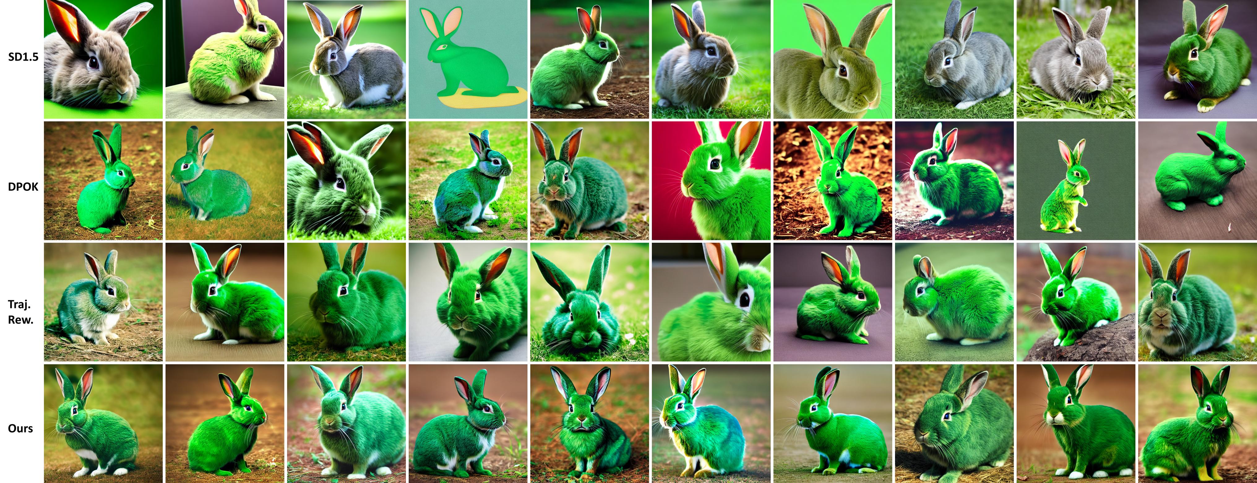
Figure 8: Single prompt experiment: randomly sampled generated images for the prompt “A green colored rabbit.”, from our method and the baselines in Fig. 3. “Traj. Rew.” denotes the classical DPO-style objective of assuming trajectory-level reward (Section 2.2).

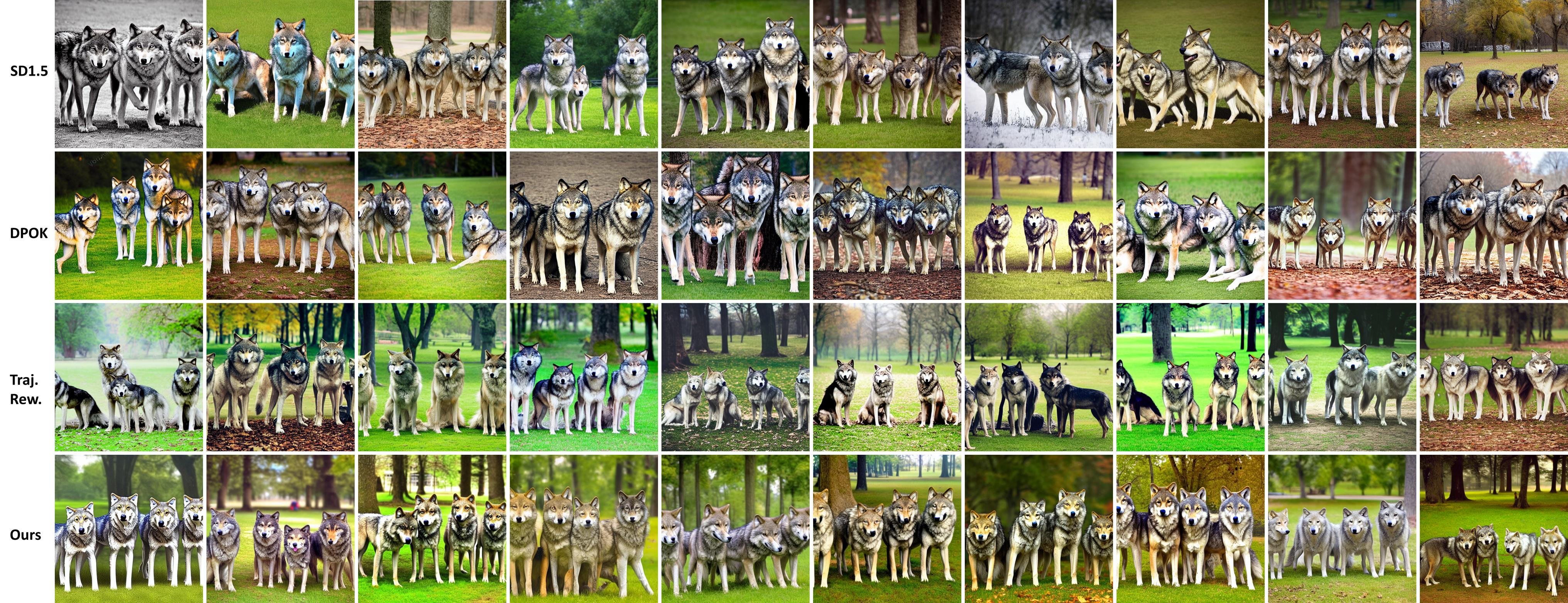
Figure 9: Single prompt experiment: randomly sampled generated images for the prompt “Four wolves in the park.”, from our method and the baselines in Fig. 3. “Traj. Rew.” denotes the classical DPO-style objective of assuming trajectory-level reward (Section 2.2).

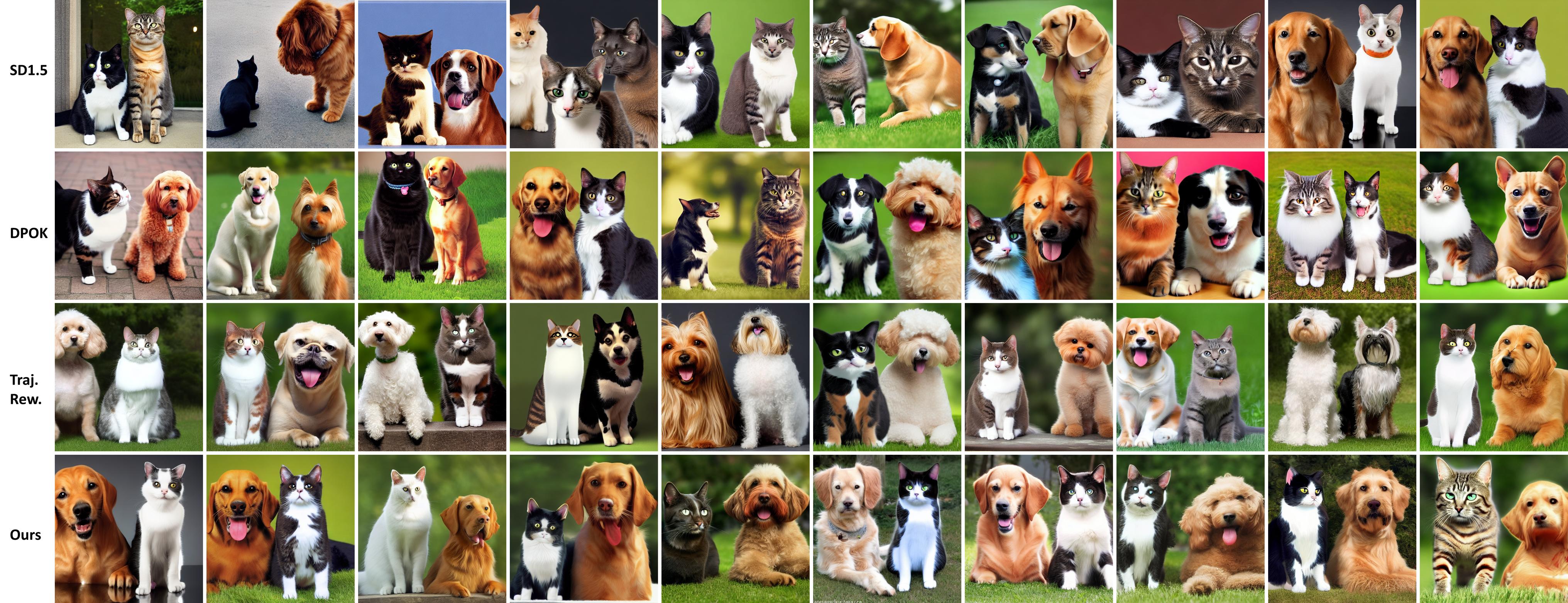
Figure 10: Single prompt experiment: randomly sampled generated images for the prompt “A cat and a dog.”, from our method and the baselines in Fig. 3. “Traj. Rew.” denotes the classical DPO-style objective of assuming trajectory-level reward (Section 2.2).

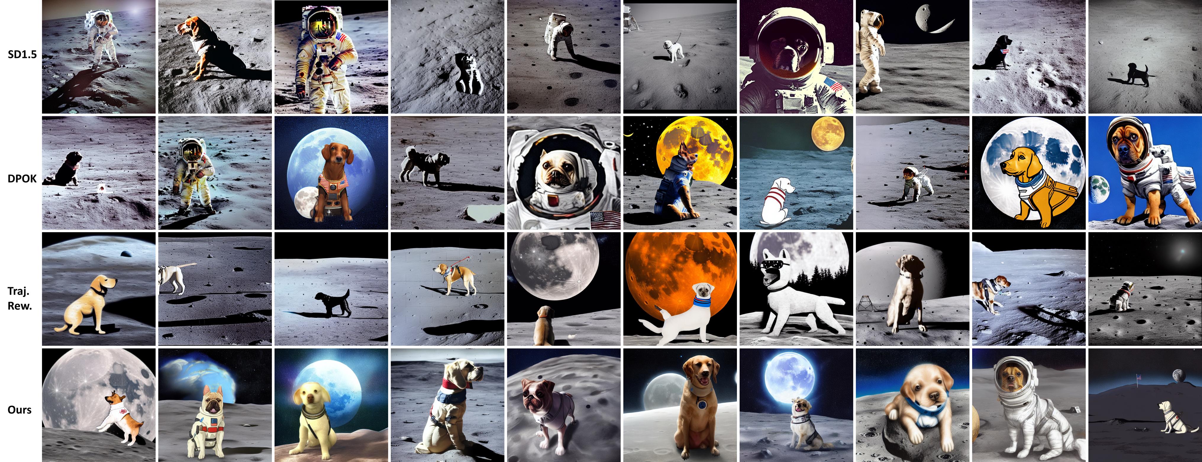
Figure 11: Single prompt experiment: randomly sampled generated images for the prompt “A dog on the moon.”, from our method and the baselines in Fig. 3. “Traj. Rew.” denotes the classical DPO-style objective of assuming trajectory-level reward (Section 2.2).

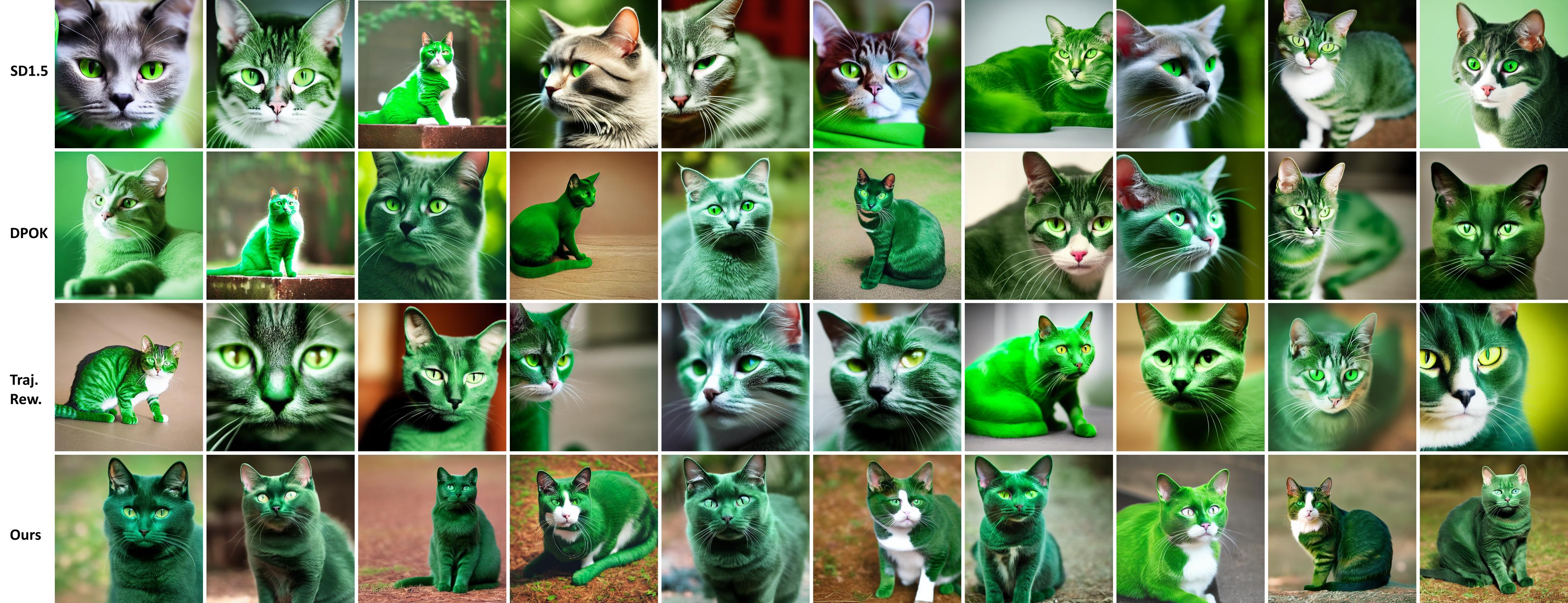
Figure 12: Single prompt experiment: randomly sampled generated images for the prompt “A green colored cat.”, from our method and the baselines in Fig. 3. “Traj. Rew.” denotes the classical DPO-style objective of assuming trajectory-level reward (Section 2.2).

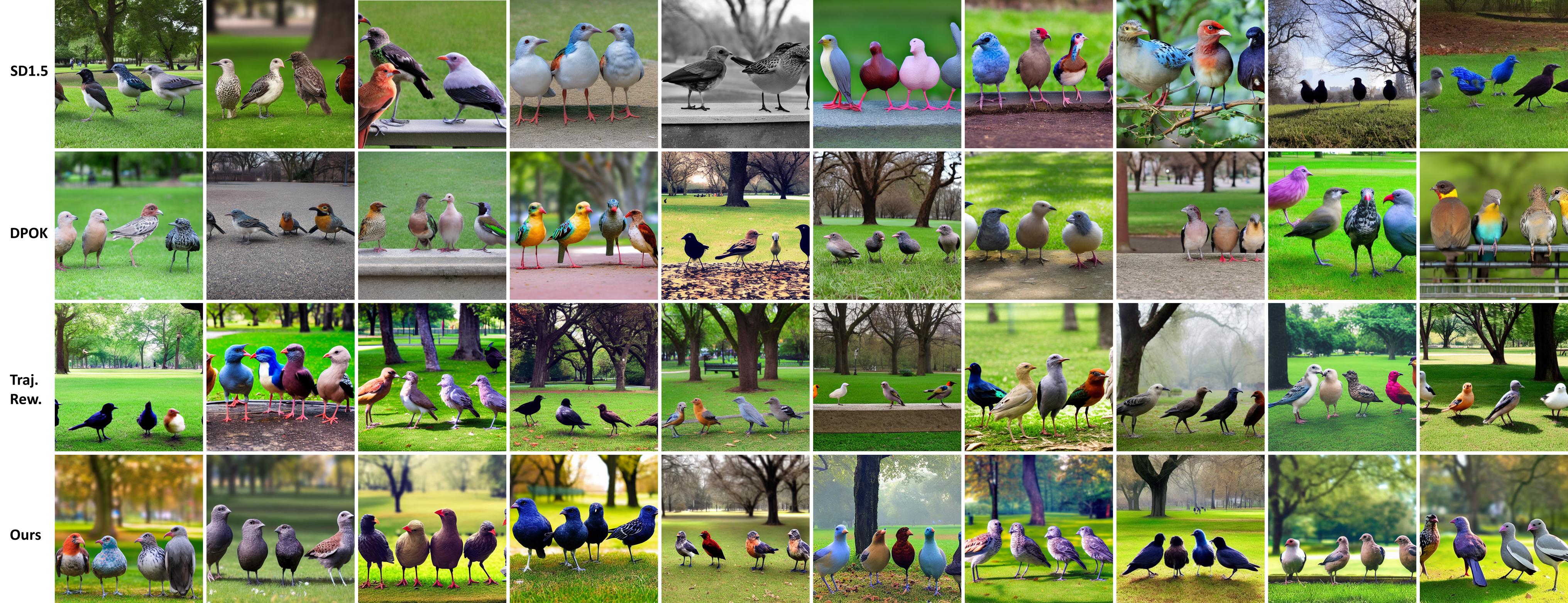
Figure 13: Single prompt experiment: randomly sampled generated images for the prompt “Four birds in the park.”, from our method and the baselines in Fig. 3. “Traj. Rew.” denotes the classical DPO-style objective of assuming trajectory-level reward (Section 2.2).

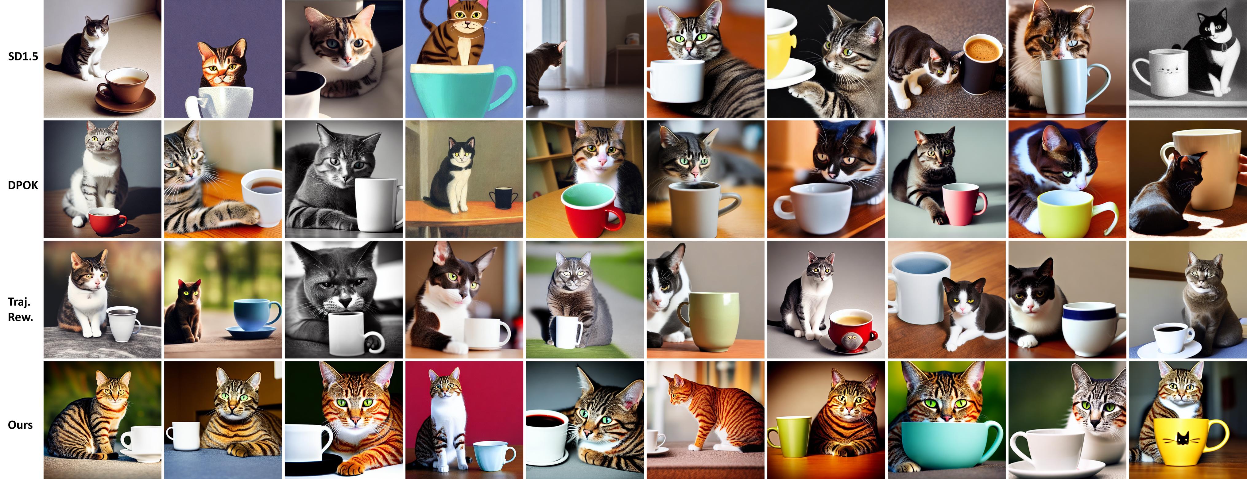
Figure 14: Single prompt experiment: randomly sampled generated images for the prompt “A cat and a cup.”, from our method and the baselines in Fig. 3. “Traj. Rew.” denotes the classical DPO-style objective of assuming trajectory-level reward (Section 2.2).

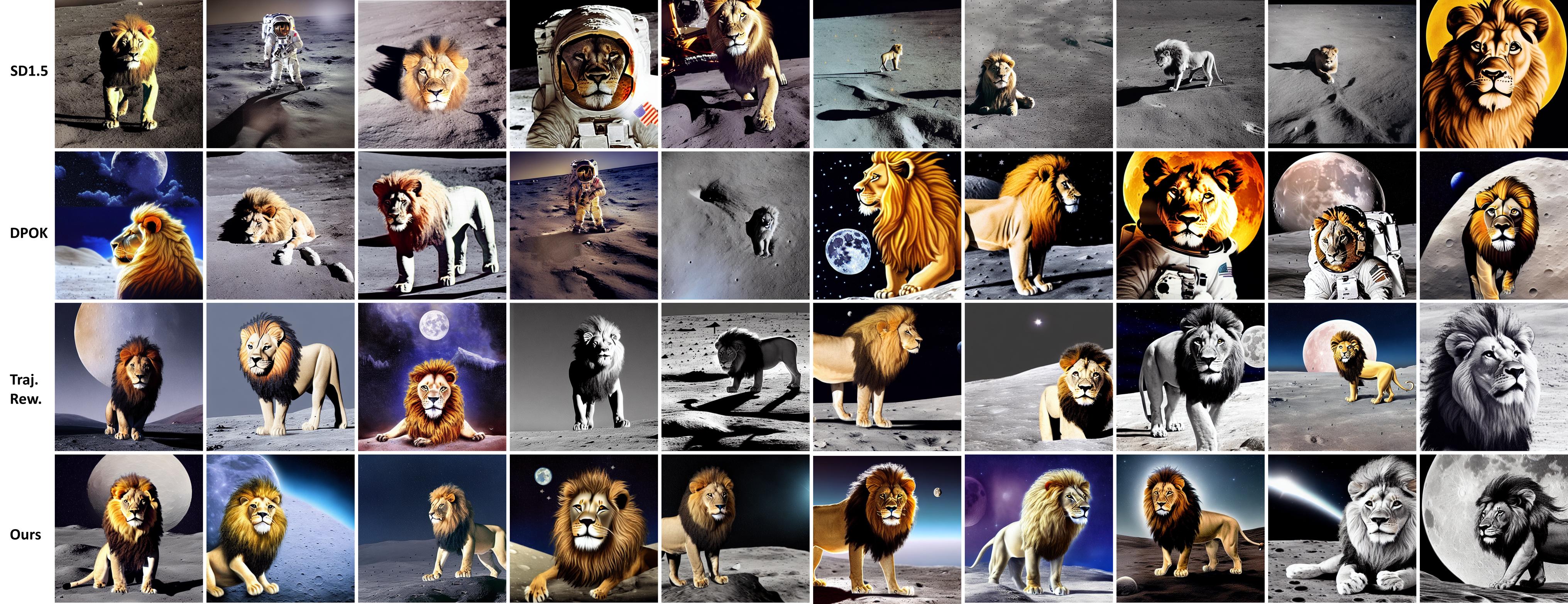
Figure 15: Single prompt experiment: randomly sampled generated images for the prompt “A lion on the moon.”, from our method and the baselines in Fig. 3. “Traj. Rew.” denotes the classical DPO-style objective of assuming trajectory-level reward (Section 2.2).

E.2 More Images from the Multiple Prompt Experiment

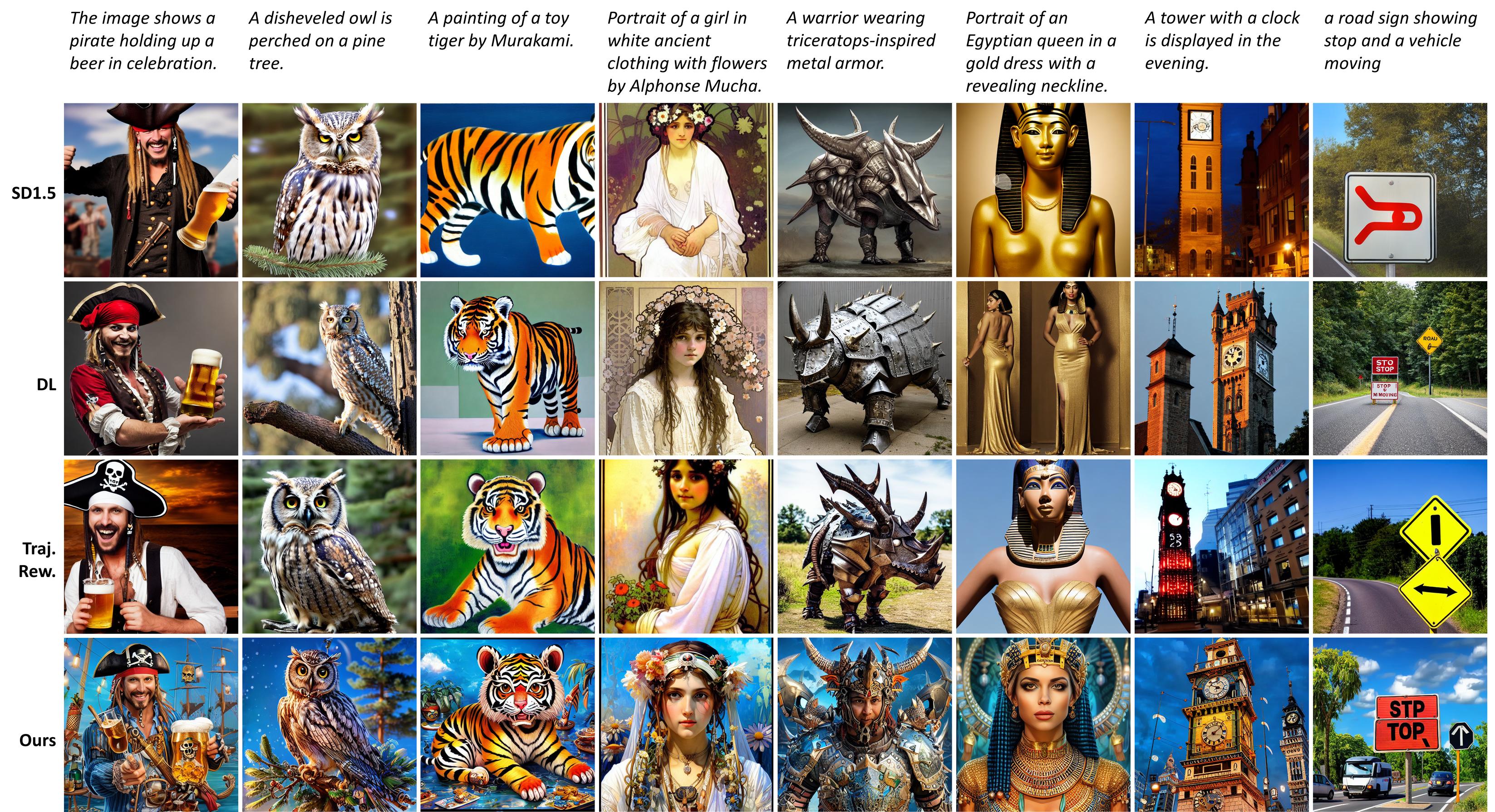
Figure 16: Multiple prompt experiment: generated images from our method and the baselines in Fig. 4 on randomly sampled prompts from the HPSv2 test set. “DL” denotes Dreamlike Photoreal 2.0, the best baseline from the HPSv2 paper. “Traj. Rew.” denotes the classical DPO-style objective of assuming trajectory-level reward (Section 2.2).

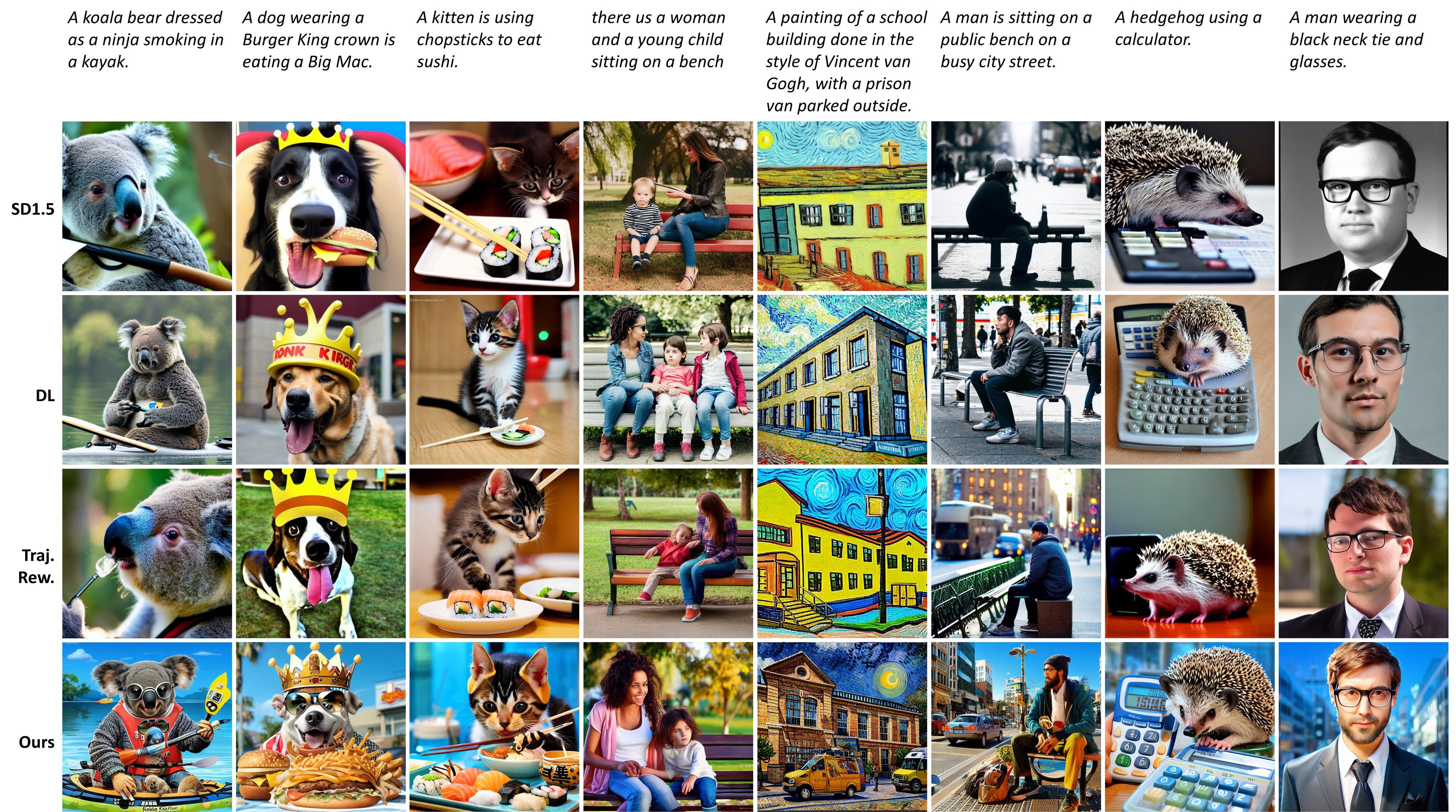
Figure 17: Multiple prompt experiment: generated images from our method and the baselines in Fig. 4 on randomly sampled prompts from the HPSv2 test set. “DL” denotes Dreamlike Photoreal 2.0, the best baseline from the HPSv2 paper. “Traj. Rew.” denotes the classical DPO-style objective of assuming trajectory-level reward (Section 2.2).

Figure 18: Multiple prompt experiment: generated images from our method and the baselines in Fig. 4 on randomly sampled prompts from the HPSv2 test set. “DL” denotes Dreamlike Photoreal 2.0, the best baseline from the HPSv2 paper. “Traj. Rew.” denotes the classical DPO-style objective of assuming trajectory-level reward (Section 2.2).

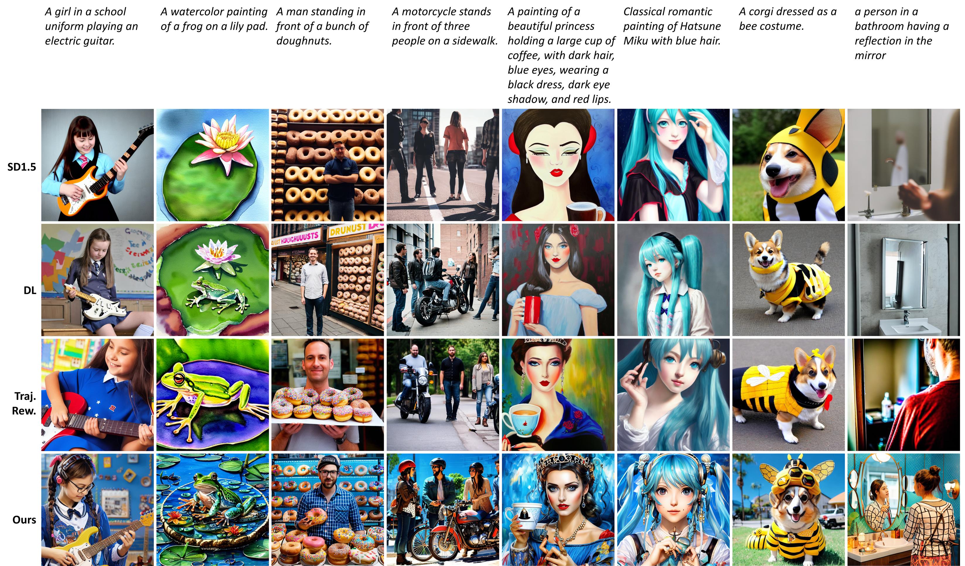
Figure 19: Multiple prompt experiment: generated images from our method and the baselines in Fig. 4 on randomly sampled prompts from the HPSv2 test set. “DL” denotes Dreamlike Photoreal 2.0, the best baseline from the HPSv2 paper. “Traj. Rew.” denotes the classical DPO-style objective of assuming trajectory-level reward (Section 2.2).

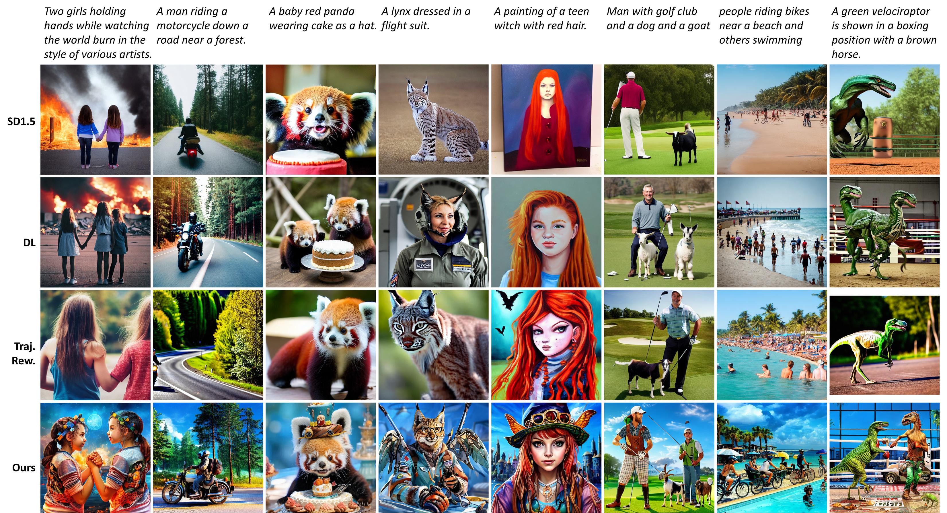
Figure 20: Multiple prompt experiment: generated images from our method and the baselines in Fig. 4 on randomly sampled prompts from the HPSv2 test set. “DL” denotes Dreamlike Photoreal 2.0, the best baseline from the HPSv2 paper. “Traj. Rew.” denotes the classical DPO-style objective of assuming trajectory-level reward (Section 2.2).

E.3 More Generation Trajectories

Recall that for all generation trajectories, we show the (decoded) $\hat{\bm{x}}_{0}$ predicted from the latents at the specified timesteps of the diffusion reverse chain. A brief discussion on each figure is in its caption.

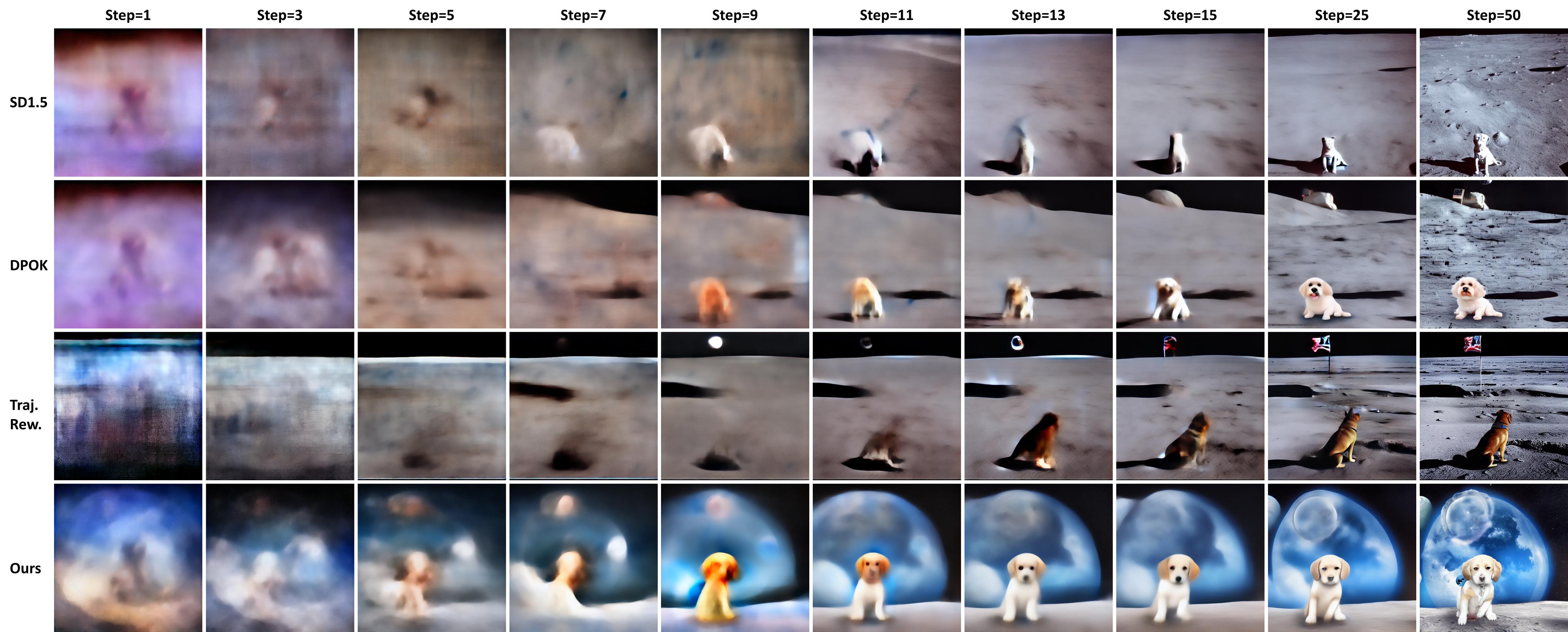
Figure 21: Generation trajectories for the prompt “A dog on the moon.”, correspond to the images in Fig. 3 from our method and the baselines. “Traj. Rew.” denotes the classical DPO-style objective of assuming trajectory-level reward (Section 2.2). Our method generates the required shape of a dog as early as at Step $11$, when the shapes of the baselines are mostly unrecognizable. At Step $13$, our method is able to give a rather complete generation for the input prompt. Subsequent steps in the reverse chain are then allocated to polish the image details, leading to a better final image.

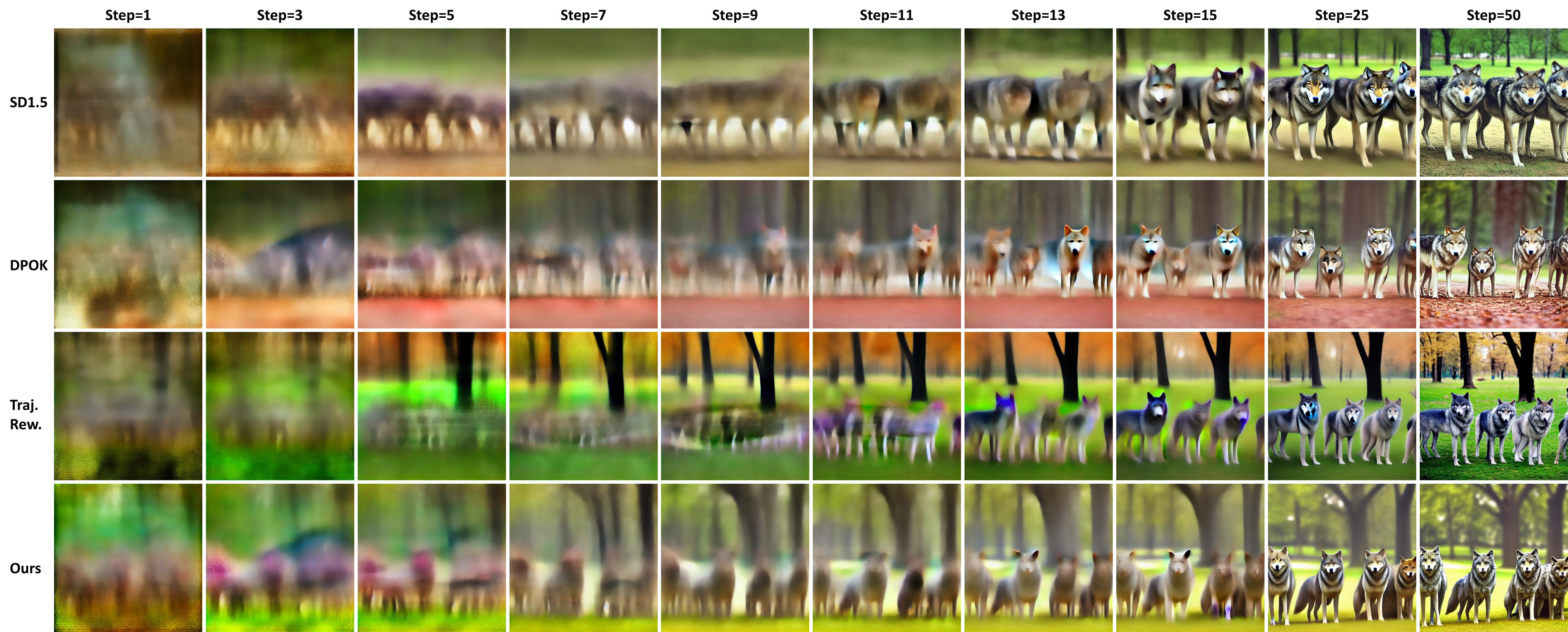
Figure 22: Generation trajectories for the prompt “Four wolves in the park.”, correspond to the images in Fig. 3 from our method and the baselines. “Traj. Rew.” denotes the classical DPO-style objective of assuming trajectory-level reward (Section 2.2). Our method generates outlines of the requires shapes (four wolves) as early as at Steps $9$ and $11$, earlier than the baselines especially the “Traj. Rew.”.

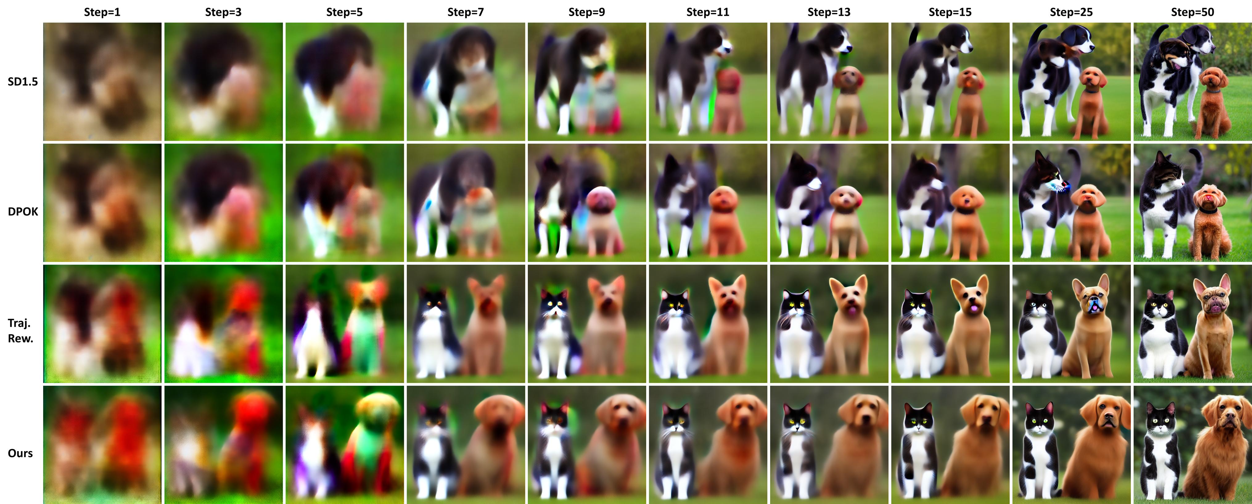
Figure 23: Generation trajectories for the prompt “A cat and a dog.”, correspond to the images in Fig. 3 from our method and the baselines. “Traj. Rew.” denotes the classical DPO-style objective of assuming trajectory-level reward (Section 2.2). Our method generates the outlines of the required shapes as fast as at Steps $3$ and $5$, especially when compared to the baselines DPOK and raw SD1.5. This helps our method in generating a more reasonable and better final image.

References

- Abdolmaleki et al. (2018) Abbas Abdolmaleki, Jost Tobias Springenberg, Yuval Tassa, Remi Munos, Nicolas Heess, and Martin Riedmiller. Maximum a posteriori policy optimisation. In International Conference on Learning Representations, 2018. URL https://openreview.net/forum?id=S1ANxQW0b.
- Akrour et al. (2011) Riad Akrour, Marc Schoenauer, and Michele Sebag. Preference-based policy learning. In Machine Learning and Knowledge Discovery in Databases: European Conference, ECML PKDD 2011, Athens, Greece, September 5-9, 2011. Proceedings, Part I 11, pages 12–27. Springer, 2011.
- Akrour et al. (2012) Riad Akrour, Marc Schoenauer, and Michèle Sebag. April: Active preference learning-based reinforcement learning. In Machine Learning and Knowledge Discovery in Databases: European Conference, ECML PKDD 2012, Bristol, UK, September 24-28, 2012. Proceedings, Part II 23, pages 116–131. Springer, 2012.
- Andrychowicz et al. (2017) Marcin Andrychowicz, Filip Wolski, Alex Ray, Jonas Schneider, Rachel Fong, Peter Welinder, Bob McGrew, Josh Tobin, OpenAI Pieter Abbeel, and Wojciech Zaremba. Hindsight experience replay. Advances in neural information processing systems, 30, 2017.
- Azar et al. (2023) Mohammad Gheshlaghi Azar, Mark Rowland, Bilal Piot, Daniel Guo, Daniele Calandriello, Michal Valko, and Rémi Munos. A general theoretical paradigm to understand learning from human preferences. arXiv preprint arXiv:2310.12036, 2023.
- Bai et al. (2022a) Yuntao Bai, Andy Jones, Kamal Ndousse, Amanda Askell, Anna Chen, Nova DasSarma, Dawn Drain, Stanislav Fort, Deep Ganguli, Tom Henighan, et al. Training a helpful and harmless assistant with reinforcement learning from human feedback. arXiv preprint arXiv:2204.05862, 2022a.
- Bai et al. (2022b) Yuntao Bai, Saurav Kadavath, Sandipan Kundu, Amanda Askell, Jackson Kernion, Andy Jones, Anna Chen, Anna Goldie, Azalia Mirhoseini, Cameron McKinnon, et al. Constitutional ai: Harmlessness from ai feedback. arXiv preprint arXiv:2212.08073, 2022b.
- Betker et al. (2023) James Betker, Gabriel Goh, Li Jing, Tim Brooks, Jianfeng Wang, Linjie Li, Long Ouyang, Juntang Zhuang, Joyce Lee, Yufei Guo, et al. Improving image generation with better captions. Computer Science. https://cdn.openai.com/papers/dall-e-3.pdf, 2:3, 2023.
- Bıyık et al. (2019) Erdem Bıyık, Daniel A Lazar, Dorsa Sadigh, and Ramtin Pedarsani. The green choice: Learning and influencing human decisions on shared roads. In 2019 IEEE 58th conference on decision and control (CDC), pages 347–354. IEEE, 2019.
- Black et al. (2023) Kevin Black, Michael Janner, Yilun Du, Ilya Kostrikov, and Sergey Levine. Training diffusion models with reinforcement learning. arXiv preprint arXiv:2305.13301, 2023.
- Bradley and Terry (1952) Ralph Allan Bradley and Milton E Terry. Rank analysis of incomplete block designs: I. the method of paired comparisons. Biometrika, 39(3/4):324–345, 1952.
- Brown et al. (2019) Daniel Brown, Wonjoon Goo, Prabhat Nagarajan, and Scott Niekum. Extrapolating beyond suboptimal demonstrations via inverse reinforcement learning from observations. In International conference on machine learning, pages 783–792. PMLR, 2019.
- Brown et al. (2020) Daniel S Brown, Wonjoon Goo, and Scott Niekum. Better-than-demonstrator imitation learning via automatically-ranked demonstrations. In Conference on robot learning, pages 330–359. PMLR, 2020.
- Castricato et al. (2022) Louis Castricato, Alexander Havrilla, Shahbuland Matiana, Michael Pieler, Anbang Ye, Ian Yang, Spencer Frazier, and Mark Riedl. Robust preference learning for storytelling via contrastive reinforcement learning. arXiv preprint arXiv:2210.07792, 2022.
- Chen et al. (2017) Hongshen Chen, Xiaorui Liu, Dawei Yin, and Jiliang Tang. A survey on dialogue systems: Recent advances and new frontiers. Acm Sigkdd Explorations Newsletter, 19(2):25–35, 2017.
- Christiano et al. (2017) Paul F Christiano, Jan Leike, Tom Brown, Miljan Martic, Shane Legg, and Dario Amodei. Deep reinforcement learning from human preferences. Advances in neural information processing systems, 30, 2017.
- Clark et al. (2023) Kevin Clark, Paul Vicol, Kevin Swersky, and David J Fleet. Directly fine-tuning diffusion models on differentiable rewards. arXiv preprint arXiv:2309.17400, 2023.
- Dai et al. (2023) Xiaoliang Dai, Ji Hou, Chih-Yao Ma, Sam Tsai, Jialiang Wang, Rui Wang, Peizhao Zhang, Simon Vandenhende, Xiaofang Wang, Abhimanyu Dubey, et al. Emu: Enhancing image generation models using photogenic needles in a haystack. arXiv preprint arXiv:2309.15807, 2023.
- Deng et al. (2022) Mingkai Deng, Jianyu Wang, Cheng-Ping Hsieh, Yihan Wang, Han Guo, Tianmin Shu, Meng Song, Eric P Xing, and Zhiting Hu. Rlprompt: Optimizing discrete text prompts with reinforcement learning. arXiv preprint arXiv:2205.12548, 2022.
- Devlin et al. (2018) Jacob Devlin, Ming-Wei Chang, Kenton Lee, and Kristina Toutanova. Bert: Pre-training of deep bidirectional transformers for language understanding. arXiv preprint arXiv:1810.04805, 2018.
- Dong et al. (2023) Hanze Dong, Wei Xiong, Deepanshu Goyal, Rui Pan, Shizhe Diao, Jipeng Zhang, Kashun Shum, and T. Zhang. Raft: Reward ranked finetuning for generative foundation model alignment. ArXiv, abs/2304.06767, 2023. URL https://api.semanticscholar.org/CorpusID:258170300.
- Ethayarajh et al. (2023) Kawin Ethayarajh, Winnie Xu, Dan Jurafsky, and Douwe Kiela. Human-centered loss functions (halos). Technical report, Contextual AI, 2023. URL https://github.com/ContextualAI/HALOs/blob/main/assets/report.pdf.
- Fan and Lee (2023) Ying Fan and Kangwook Lee. Optimizing ddpm sampling with shortcut fine-tuning. In International Conference on Machine Learning, 2023. URL https://api.semanticscholar.org/CorpusID:256415971.
- Fan et al. (2023) Ying Fan, Olivia Watkins, Yuqing Du, Hao Liu, Moonkyung Ryu, Craig Boutilier, Pieter Abbeel, Mohammad Ghavamzadeh, Kangwook Lee, and Kimin Lee. Dpok: Reinforcement learning for fine-tuning text-to-image diffusion models. arXiv preprint arXiv:2305.16381, 2023.
- Feng et al. (2023) Yihao Feng, Shentao Yang, Shujian Zhang, Jianguo Zhang, Caiming Xiong, Mingyuan Zhou, and Huan Wang. Fantastic rewards and how to tame them: A case study on reward learning for task-oriented dialogue systems. In The Eleventh International Conference on Learning Representations, 2023.
- Finn et al. (2016) Chelsea Finn, Paul Francis Christiano, P. Abbeel, and Sergey Levine. A connection between generative adversarial networks, inverse reinforcement learning, and energy-based models. ArXiv, abs/1611.03852, 2016.
- Fürnkranz et al. (2012) Johannes Fürnkranz, Eyke Hüllermeier, Weiwei Cheng, and Sang-Hyeun Park. Preference-based reinforcement learning: a formal framework and a policy iteration algorithm. Machine learning, 89:123–156, 2012.
- Guo et al. (2022) Han Guo, Bowen Tan, Zhengzhong Liu, Eric Xing, and Zhiting Hu. Efficient (soft) q-learning for text generation with limited good data. Findings of the Association for Computational Linguistics: EMNLP 2022, pages 6969–6991, 2022.
- Guo et al. (2018) Jiaxian Guo, Sidi Lu, Han Cai, Weinan Zhang, Yong Yu, and Jun Wang. Long text generation via adversarial training with leaked information. In Proceedings of the AAAI conference on artificial intelligence, volume 32, 2018.
- Hao et al. (2022) Yaru Hao, Zewen Chi, Li Dong, and Furu Wei. Optimizing prompts for text-to-image generation. ArXiv, abs/2212.09611, 2022. URL https://api.semanticscholar.org/CorpusID:254853701.
- Hejna and Sadigh (2023a) Donald Joseph Hejna and Dorsa Sadigh. Few-shot preference learning for human-in-the-loop rl. In Conference on Robot Learning, pages 2014–2025. PMLR, 2023a.
- Hejna and Sadigh (2023b) Joey Hejna and Dorsa Sadigh. Inverse preference learning: Preference-based rl without a reward function. arXiv preprint arXiv:2305.15363, 2023b.
- Hejna et al. (2023) Joey Hejna, Rafael Rafailov, Harshit Sikchi, Chelsea Finn, Scott Niekum, W Bradley Knox, and Dorsa Sadigh. Contrastive prefence learning: Learning from human feedback without rl. arXiv preprint arXiv:2310.13639, 2023.
- Ho and Salimans (2022) Jonathan Ho and Tim Salimans. Classifier-free diffusion guidance. arXiv preprint arXiv:2207.12598, 2022.
- Ho et al. (2020) Jonathan Ho, Ajay Jain, and Pieter Abbeel. Denoising diffusion probabilistic models. Advances in neural information processing systems, 33:6840–6851, 2020.
- Hu et al. (2021) Edward J Hu, Yelong Shen, Phillip Wallis, Zeyuan Allen-Zhu, Yuanzhi Li, Shean Wang, Lu Wang, and Weizhu Chen. Lora: Low-rank adaptation of large language models. arXiv preprint arXiv:2106.09685, 2021.
- Ibarz et al. (2018) Borja Ibarz, Jan Leike, Tobias Pohlen, Geoffrey Irving, Shane Legg, and Dario Amodei. Reward learning from human preferences and demonstrations in atari. Advances in neural information processing systems, 31, 2018.
- Jaques et al. (2019) Natasha Jaques, Asma Ghandeharioun, Judy Hanwen Shen, Craig Ferguson, À. Lapedriza, Noah J. Jones, S. Gu, and Rosalind W. Picard. Way Off-Policy Batch Deep Reinforcement Learning of Implicit Human Preferences in Dialog. ArXiv, abs/1907.00456, 2019.
- Jaques et al. (2020) Natasha Jaques, Judy Hanwen Shen, Asma Ghandeharioun, Craig Ferguson, Agata Lapedriza, Noah Jones, Shixiang Shane Gu, and Rosalind Picard. Human-centric dialog training via offline reinforcement learning. arXiv preprint arXiv:2010.05848, 2020.
- Kakade and Langford (2002) Sham Kakade and John Langford. Approximately optimal approximate reinforcement learning. In Proceedings of the Nineteenth International Conference on Machine Learning, pages 267–274, 2002.
- Karras et al. (2022) Tero Karras, Miika Aittala, Timo Aila, and Samuli Laine. Elucidating the design space of diffusion-based generative models. Advances in Neural Information Processing Systems, 35:26565–26577, 2022.
- Kim et al. (2023) Changyeon Kim, Jongjin Park, Jinwoo Shin, Honglak Lee, Pieter Abbeel, and Kimin Lee. Preference transformer: Modeling human preferences using transformers for RL. In The Eleventh International Conference on Learning Representations, 2023. URL https://openreview.net/forum?id=Peot1SFDX0.
- Kirstain et al. (2023) Yuval Kirstain, Adam Polyak, Uriel Singer, Shahbuland Matiana, Joe Penna, and Omer Levy. Pick-a-pic: An open dataset of user preferences for text-to-image generation. arXiv preprint arXiv:2305.01569, 2023.
- Knox et al. (2022) W. B. Knox, Stephane Hatgis-Kessell, Serena Booth, Scott Niekum, Peter Stone, and Alessandro Allievi. Models of human preference for learning reward functions. ArXiv, abs/2206.02231, 2022. URL https://api.semanticscholar.org/CorpusID:249395243.
- Knox et al. (2023) W. B. Knox, Stephane Hatgis-Kessell, Sigurdur O. Adalgeirsson, Serena Booth, Anca D. Dragan, Peter Stone, and Scott Niekum. Learning optimal advantage from preferences and mistaking it for reward. ArXiv, abs/2310.02456, 2023. URL https://api.semanticscholar.org/CorpusID:263620440.
- Korbak et al. (2023) Tomasz Korbak, Kejian Shi, Angelica Chen, Rasika Bhalerao, Christopher L Buckley, Jason Phang, Samuel R Bowman, and Ethan Perez. Pretraining language models with human preferences. arXiv preprint arXiv:2302.08582, 2023.
- Kwan et al. (2022) Wai-Chung Kwan, Hongru Wang, Huimin Wang, and Kam-Fai Wong. A survey on recent advances and challenges in reinforcement learningmethods for task-oriented dialogue policy learning. arXiv preprint arXiv:2202.13675, 2022.
- Laidlaw et al. (2023) Cassidy Laidlaw, Stuart Russell, and Anca Dragan. Bridging rl theory and practice with the effective horizon. arXiv preprint arXiv:2304.09853, 2023.
- Le et al. (2022) Hung Le, Yue Wang, Akhilesh Deepak Gotmare, Silvio Savarese, and Steven Chu Hong Hoi. Coderl: Mastering code generation through pretrained models and deep reinforcement learning. Advances in Neural Information Processing Systems, 35:21314–21328, 2022.
- Lee et al. (2021) Kimin Lee, Laura M. Smith, and P. Abbeel. Pebble: Feedback-efficient interactive reinforcement learning via relabeling experience and unsupervised pre-training. In International Conference on Machine Learning, 2021. URL https://api.semanticscholar.org/CorpusID:235377145.
- Lee et al. (2023a) Kimin Lee, Hao Liu, Moonkyung Ryu, Olivia Watkins, Yuqing Du, Craig Boutilier, P. Abbeel, Mohammad Ghavamzadeh, and Shixiang Shane Gu. Aligning text-to-image models using human feedback. ArXiv, abs/2302.12192, 2023a. URL https://api.semanticscholar.org/CorpusID:257102772.
- Lee et al. (2023b) Kimin Lee, Hao Liu, Moonkyung Ryu, Olivia Watkins, Yuqing Du, Craig Boutilier, Pieter Abbeel, Mohammad Ghavamzadeh, and Shixiang Shane Gu. Aligning text-to-image models using human feedback. arXiv preprint arXiv:2302.12192, 2023b.
- Lewis et al. (2019) Mike Lewis, Yinhan Liu, Naman Goyal, Marjan Ghazvininejad, Abdelrahman Mohamed, Omer Levy, Ves Stoyanov, and Luke Zettlemoyer. Bart: Denoising sequence-to-sequence pre-training for natural language generation, translation, and comprehension. arXiv preprint arXiv:1910.13461, 2019.
- Lillicrap et al. (2016) T. Lillicrap, Jonathan J. Hunt, A. Pritzel, N. Heess, T. Erez, Yuval Tassa, D. Silver, and Daan Wierstra. Continuous Control with Deep Reinforcement Learning. CoRR, abs/1509.02971, 2016.
- Lin et al. (2017) Kevin Lin, Dianqi Li, Xiaodong He, Zhengyou Zhang, and Ming-Ting Sun. Adversarial ranking for language generation. Advances in neural information processing systems, 30, 2017.
- Liu et al. (2019) Hao Liu, Alexander Trott, Richard Socher, and Caiming Xiong. Competitive experience replay. In International Conference on Learning Representations, 2019.
- Loshchilov and Hutter (2017) Ilya Loshchilov and Frank Hutter. Decoupled weight decay regularization. arXiv preprint arXiv:1711.05101, 2017.
- Lu et al. (2022) Ximing Lu, Sean Welleck, Liwei Jiang, Jack Hessel, Lianhui Qin, Peter West, Prithviraj Ammanabrolu, and Yejin Choi. Quark: Controllable text generation with reinforced unlearning. arXiv preprint arXiv:2205.13636, 2022.
- Marbach and Tsitsiklis (2003) Peter Marbach and John N Tsitsiklis. Approximate gradient methods in policy-space optimization of markov reward processes. Discrete Event Dynamic Systems, 13:111–148, 2003.
- Menick et al. (2022) Jacob Menick, Maja Trebacz, Vladimir Mikulik, John Aslanides, Francis Song, Martin Chadwick, Mia Glaese, Susannah Young, Lucy Campbell-Gillingham, Geoffrey Irving, et al. Teaching language models to support answers with verified quotes. arXiv preprint arXiv:2203.11147, 2022.
- Mnih et al. (2013) Volodymyr Mnih, Koray Kavukcuoglu, David Silver, Alex Graves, Ioannis Antonoglou, Daan Wierstra, and Martin Riedmiller. Playing atari with deep reinforcement learning. arXiv preprint arXiv:1312.5602, 2013.
- Ng et al. (1999) Andrew Y Ng, Daishi Harada, and Stuart Russell. Policy invariance under reward transformations: Theory and application to reward shaping. In Icml, volume 99, pages 278–287. Citeseer, 1999.
- OpenAI (2023) OpenAI. Gpt-4 technical report, 2023.
- Ouyang et al. (2022) Long Ouyang, Jeff Wu, Xu Jiang, Diogo Almeida, Carroll L Wainwright, Pamela Mishkin, Chong Zhang, Sandhini Agarwal, Katarina Slama, Alex Ray, et al. Training language models to follow instructions with human feedback. arXiv preprint arXiv:2203.02155, 2022.
- Paulus et al. (2017) Romain Paulus, Caiming Xiong, and Richard Socher. A deep reinforced model for abstractive summarization. arXiv preprint arXiv:1705.04304, 2017.
- Peng et al. (2019) Xue Bin Peng, Aviral Kumar, Grace Zhang, and Sergey Levine. Advantage-weighted regression: Simple and scalable off-policy reinforcement learning. arXiv preprint arXiv:1910.00177, 2019.
- Peters et al. (2010) Jan Peters, Katharina Mulling, and Yasemin Altun. Relative entropy policy search. In Proceedings of the AAAI Conference on Artificial Intelligence, volume 24, pages 1607–1612, 2010.
- Podell et al. (2023) Dustin Podell, Zion English, Kyle Lacey, Andreas Blattmann, Tim Dockhorn, Jonas Müller, Joe Penna, and Robin Rombach. Sdxl: Improving latent diffusion models for high-resolution image synthesis. arXiv preprint arXiv:2307.01952, 2023.
- Prabhudesai et al. (2023) Mihir Prabhudesai, Anirudh Goyal, Deepak Pathak, and Katerina Fragkiadaki. Aligning text-to-image diffusion models with reward backpropagation. arXiv preprint arXiv:2310.03739, 2023.
- Radford et al. (2019) Alec Radford, Jeffrey Wu, Rewon Child, David Luan, Dario Amodei, Ilya Sutskever, et al. Language models are unsupervised multitask learners. OpenAI blog, 1(8):9, 2019.
- Rafailov et al. (2023) Rafael Rafailov, Archit Sharma, Eric Mitchell, Christopher D Manning, Stefano Ermon, and Chelsea Finn. Direct preference optimization: Your language model is secretly a reward model. In Thirty-seventh Conference on Neural Information Processing Systems, 2023. URL https://openreview.net/forum?id=HPuSIXJaa9.
- Ramachandran et al. (2021) Govardana Sachithanandam Ramachandran, Kazuma Hashimoto, and Caiming Xiong. Causal-aware safe policy improvement for task-oriented dialogue. arXiv preprint arXiv:2103.06370, 2021.
- Ramamurthy et al. (2022) Rajkumar Ramamurthy, Prithviraj Ammanabrolu, Kianté Brantley, Jack Hessel, Rafet Sifa, Christian Bauckhage, Hannaneh Hajishirzi, and Yejin Choi. Is reinforcement learning (not) for natural language processing?: Benchmarks, baselines, and building blocks for natural language policy optimization. arXiv preprint arXiv:2210.01241, 2022.
- Ramesh et al. (2022) Aditya Ramesh, Prafulla Dhariwal, Alex Nichol, Casey Chu, and Mark Chen. Hierarchical text-conditional image generation with clip latents. arXiv preprint arXiv:2204.06125, 1(2):3, 2022.
- Ranzato et al. (2015) Marc’Aurelio Ranzato, Sumit Chopra, Michael Auli, and Wojciech Zaremba. Sequence level training with recurrent neural networks. arXiv preprint arXiv:1511.06732, 2015.
- Rennie et al. (2017) Steven J Rennie, Etienne Marcheret, Youssef Mroueh, Jerret Ross, and Vaibhava Goel. Self-critical sequence training for image captioning. In Proceedings of the IEEE conference on computer vision and pattern recognition, pages 7008–7024, 2017.
- Rombach et al. (2022) Robin Rombach, Andreas Blattmann, Dominik Lorenz, Patrick Esser, and Björn Ommer. High-resolution image synthesis with latent diffusion models. In Proceedings of the IEEE/CVF conference on computer vision and pattern recognition, pages 10684–10695, 2022.
- Ronneberger et al. (2015) Olaf Ronneberger, Philipp Fischer, and Thomas Brox. U-net: Convolutional networks for biomedical image segmentation. In Medical Image Computing and Computer-Assisted Intervention–MICCAI 2015: 18th International Conference, Munich, Germany, October 5-9, 2015, Proceedings, Part III 18, pages 234–241. Springer, 2015.
- Russell (1998) Stuart Russell. Learning agents for uncertain environments. In Proceedings of the eleventh annual conference on Computational learning theory, pages 101–103, 1998.
- Ryang and Abekawa (2012) Seonggi Ryang and Takeshi Abekawa. Framework of automatic text summarization using reinforcement learning. In Proceedings of the 2012 Joint Conference on Empirical Methods in Natural Language Processing and Computational Natural Language Learning, pages 256–265, Jeju Island, Korea, July 2012. Association for Computational Linguistics. URL https://aclanthology.org/D12-1024.
- Saharia et al. (2022) Chitwan Saharia, William Chan, Saurabh Saxena, Lala Li, Jay Whang, Emily L Denton, Kamyar Ghasemipour, Raphael Gontijo Lopes, Burcu Karagol Ayan, Tim Salimans, et al. Photorealistic text-to-image diffusion models with deep language understanding. Advances in Neural Information Processing Systems, 35:36479–36494, 2022.
- Schuhmann et al. (2022) Christoph Schuhmann, Romain Beaumont, Richard Vencu, Cade Gordon, Ross Wightman, Mehdi Cherti, Theo Coombes, Aarush Katta, Clayton Mullis, Mitchell Wortsman, et al. Laion-5b: An open large-scale dataset for training next generation image-text models. Advances in Neural Information Processing Systems, 35:25278–25294, 2022.
- Schulman et al. (2015) J. Schulman, Sergey Levine, P. Abbeel, Michael I. Jordan, and Philipp Moritz. Trust Region Policy Optimization. ArXiv, abs/1502.05477, 2015.
- Schulman et al. (2017) John Schulman, Filip Wolski, Prafulla Dhariwal, Alec Radford, and Oleg Klimov. Proximal policy optimization algorithms. arXiv preprint arXiv:1707.06347, 2017.
- Segalis et al. (2023) Eyal Segalis, Dani Valevski, Danny Lumen, Yossi Matias, and Yaniv Leviathan. A picture is worth a thousand words: Principled recaptioning improves image generation. arXiv preprint arXiv:2310.16656, 2023.
- Shi et al. (2018) Zhan Shi, Xinchi Chen, Xipeng Qiu, and Xuanjing Huang. Toward diverse text generation with inverse reinforcement learning. arXiv preprint arXiv:1804.11258, 2018.
- Shin et al. (2021) Daniel Shin, Daniel S Brown, and Anca D Dragan. Offline preference-based apprenticeship learning. arXiv preprint arXiv:2107.09251, 2021.
- Shu et al. (2021) Raphael Shu, Kang Min Yoo, and Jung-Woo Ha. Reward optimization for neural machine translation with learned metrics. arXiv preprint arXiv:2104.07541, 2021.
- Snell et al. (2022) Charlie Snell, Ilya Kostrikov, Yi Su, Mengjiao Yang, and Sergey Levine. Offline rl for natural language generation with implicit language q learning. arXiv preprint arXiv:2206.11871, 2022.
- Sohl-Dickstein et al. (2015) Jascha Sohl-Dickstein, Eric Weiss, Niru Maheswaranathan, and Surya Ganguli. Deep unsupervised learning using nonequilibrium thermodynamics. In International conference on machine learning, pages 2256–2265. PMLR, 2015.
- Song et al. (2020) Jiaming Song, Chenlin Meng, and Stefano Ermon. Denoising diffusion implicit models. arXiv preprint arXiv:2010.02502, 2020.
- Song et al. (2021) Yang Song, Jascha Sohl-Dickstein, Diederik P Kingma, Abhishek Kumar, Stefano Ermon, and Ben Poole. Score-based generative modeling through stochastic differential equations. In International Conference on Learning Representations, 2021. URL https://openreview.net/forum?id=PxTIG12RRHS.
- Stiennon et al. (2020) Nisan Stiennon, Long Ouyang, Jeffrey Wu, Daniel Ziegler, Ryan Lowe, Chelsea Voss, Alec Radford, Dario Amodei, and Paul F Christiano. Learning to summarize from human feedback. Advances in Neural Information Processing Systems, 33:3008–3021, 2020.
- Sutton and Barto (2018) Richard S Sutton and Andrew G Barto. Reinforcement learning: An introduction. MIT press, 2018.
- Takanobu et al. (2019) Ryuichi Takanobu, Hanlin Zhu, and Minlie Huang. Guided dialog policy learning: Reward estimation for multi-domain task-oriented dialog. arXiv preprint arXiv:1908.10719, 2019.
- Touvron et al. (2023) Hugo Touvron, Louis Martin, Kevin Stone, Peter Albert, Amjad Almahairi, Yasmine Babaei, Nikolay Bashlykov, Soumya Batra, Prajjwal Bhargava, Shruti Bhosale, et al. Llama 2: Open foundation and fine-tuned chat models. arXiv preprint arXiv:2307.09288, 2023.
- Tunstall et al. (2023) Lewis Tunstall, Edward Beeching, Nathan Lambert, Nazneen Rajani, Kashif Rasul, Younes Belkada, Shengyi Huang, Leandro von Werra, Clémentine Fourrier, Nathan Habib, et al. Zephyr: Direct distillation of lm alignment. arXiv preprint arXiv:2310.16944, 2023.
- Wallace et al. (2023a) Bram Wallace, Meihua Dang, Rafael Rafailov, Linqi Zhou, Aaron Lou, Senthil Purushwalkam, Stefano Ermon, Caiming Xiong, Shafiq Joty, and Nikhil Naik. Diffusion model alignment using direct preference optimization. arXiv preprint arXiv:2311.12908, 2023a.
- Wallace et al. (2023b) Bram Wallace, Akash Gokul, Stefano Ermon, and Nikhil Vijay Naik. End-to-end diffusion latent optimization improves classifier guidance. 2023 IEEE/CVF International Conference on Computer Vision (ICCV), pages 7246–7256, 2023b. URL https://api.semanticscholar.org/CorpusID:257757144.
- Wang and Vastola (2023) Binxu Wang and John J. Vastola. Diffusion models generate images like painters: an analytical theory of outline first, details later, 2023.
- Wu et al. (2023a) Xiaoshi Wu, Yiming Hao, Keqiang Sun, Yixiong Chen, Feng Zhu, Rui Zhao, and Hongsheng Li. Human preference score v2: A solid benchmark for evaluating human preferences of text-to-image synthesis. arXiv preprint arXiv:2306.09341, 2023a.
- Wu et al. (2023b) Xiaoshi Wu, Keqiang Sun, Feng Zhu, Rui Zhao, and Hongsheng Li. Human preference score: Better aligning text-to-image models with human preference. In Proceedings of the IEEE/CVF International Conference on Computer Vision, pages 2096–2105, 2023b.
- Xu et al. (2023) Jiazheng Xu, Xiao Liu, Yuchen Wu, Yuxuan Tong, Qinkai Li, Ming Ding, Jie Tang, and Yuxiao Dong. Imagereward: Learning and evaluating human preferences for text-to-image generation. arXiv preprint arXiv:2304.05977, 2023.
- Yang et al. (2022a) Shentao Yang, Yihao Feng, Shujian Zhang, and Mingyuan Zhou. Regularizing a model-based policy stationary distribution to stabilize offline reinforcement learning. In International Conference on Machine Learning, pages 24980–25006. PMLR, 2022a.
- Yang et al. (2022b) Shentao Yang, Zhendong Wang, Huangjie Zheng, Yihao Feng, and Mingyuan Zhou. A regularized implicit policy for offline reinforcement learning. arXiv preprint arXiv:2202.09673, 2022b.
- Yang et al. (2022c) Shentao Yang, Shujian Zhang, Yihao Feng, and Mingyuan Zhou. A unified framework for alternating offline model training and policy learning. In Alice H. Oh, Alekh Agarwal, Danielle Belgrave, and Kyunghyun Cho, editors, Advances in Neural Information Processing Systems, 2022c.
- Yang et al. (2023) Shentao Yang, Shujian Zhang, Congying Xia, Yihao Feng, Caiming Xiong, and Mingyuan Zhou. Preference-grounded token-level guidance for language model fine-tuning. In Thirty-seventh Conference on Neural Information Processing Systems, 2023. URL https://openreview.net/forum?id=6SRE9GZ9s6.
- Yang et al. (2018) Zichao Yang, Zhiting Hu, Chris Dyer, Eric P Xing, and Taylor Berg-Kirkpatrick. Unsupervised text style transfer using language models as discriminators. Advances in Neural Information Processing Systems, 31, 2018.
- Yu et al. (2017) Lantao Yu, Weinan Zhang, Jun Wang, and Yong Yu. Seqgan: Sequence generative adversarial nets with policy gradient. In Proceedings of the AAAI conference on artificial intelligence, volume 31, 2017.
- Yuan et al. (2023) Hongyi Yuan, Zheng Yuan, Chuanqi Tan, Wei Wang, Songfang Huang, and Fei Huang. RRHF: Rank responses to align language models with human feedback. In Thirty-seventh Conference on Neural Information Processing Systems, 2023. URL https://openreview.net/forum?id=EdIGMCHk4l.
- Zhao et al. (2023) Yao Zhao, Rishabh Joshi, Tianqi Liu, Misha Khalman, Mohammad Saleh, and Peter J Liu. Slic-hf: Sequence likelihood calibration with human feedback. arXiv preprint arXiv:2305.10425, 2023.
- Ziebart (2010) Brian D Ziebart. Modeling purposeful adaptive behavior with the principle of maximum causal entropy. Carnegie Mellon University, 2010.
- Ziebart et al. (2008) Brian D. Ziebart, Andrew Maas, J. Andrew Bagnell, and Anind K. Dey. Maximum entropy inverse reinforcement learning. In Proc. AAAI, pages 1433–1438, 2008.
- Ziegler et al. (2019) Daniel M Ziegler, Nisan Stiennon, Jeffrey Wu, Tom B Brown, Alec Radford, Dario Amodei, Paul Christiano, and Geoffrey Irving. Fine-tuning language models from human preferences. arXiv preprint arXiv:1909.08593, 2019.