Crossed Andreev Reflection in altermagnets

Abstract

Crossed Andreev reflection (CAR) is a scattering phenomenon occurring in superconductors (SCs) connected to two metallic leads, where an incident electron on one side of the SC emerges on the opposite side as a hole. Despite its significance, CAR detection is often impeded by the prevalent electron tunneling (ET), where electrons exit on the opposing side. One approach to augment CAR over ET involves employing two antiparallel ferromagnets across the SC. However, this method is constrained by the low polarization in ferromagnets and necessitates the application of a magnetic field. Altermagnets (AMs) present a promising avenue for detecting and enhancing CAR due to their distinct Fermi surfaces for each spin. Here, we propose a novel configuration utilizing two AMs rotated by $90^{\circ}$ with respect to each other on either side of an SC to enhance CAR. We calculate local and nonlocal conductivities across the AM-SC-AM junction using the Landauer-Büttiker scattering approach. Our findings reveal that in the strong phase of AMs, CAR overwhelmingly dominates nonlocal transport. In the weak phase, CAR can exhibit significant enhancement for larger values of the altermagnetic parameter compared to the scenario where AMs are in the normal metallic phase. As a function of the length of SC, the conductivities exhibit oscillations reminiscent of Fabry-Pérot interference.

I Introduction

Electrons are characterized by charge and spin. While the charge of the electrons is a characteristic used in electronics, their spin is the characteristic which has opened up a new field of study known as spintronics Wolf et al. (2001); Chappert et al. (2007); Baltz et al. (2018); Fukami et al. (2020); Hoffmann and Zhang (2022); Sinova et al. (2004); Sahoo and Soori (2023). Ferromagnets and antiferomagnets have played a central role in spintronics so farBaltz et al. (2018). In ferromagnets, a majority of spins are aligned in one direction, resulting in a net spin polarization. On the other hand, in antiferomagnets neighboring spins point in opposite direction, making the net spin polarization zero. Recently, a new class of magnetic materials known as altermagnets (AMs) have generated interest among theorists and experimentalists Šmejkal et al. (2022a, b, c); Fernandes et al. (2024); Sun et al. (2023); Yan et al. (2024); Reichlova et al. (2024). In AMs, the dispersions of the two spin sectors are separated in momentum space while maintaining a zero net spin polarization. A consequence of such feature is that even though the net spin polarization is zero in both: a metal and an AM, a junction between the two carries a net spin current on application of a voltage bias Das et al. (2023). It has been predicted that some antiferromagnets can be turned into altermagnets by the application of electric field Mazin and R. Gonzalez-Hernandez (2023).

Even in ferromagnetic metals (FMs), the dispersions for the two spins are separated, but with a net spin polarization. This property enables the use of ferromagnetic metals in detecting crossed Andreev reflection (CAR) Beckmann et al. (2004) - a phenomenon wherein an electron incident onto a superconductor from a FM gets transmitted into another FM as a hole. Hindrance to experimental observation of CAR is rooted in a competing process known as electron tunneling (ET) in which the electron transmits across the SC from one metal onto the other metal as an electron. The currents carried by ET and CAR are opposite in sign and in most cases, the current carried by ET overpowers the current carried by CAR and masks the signature of CAR Chtchelkatchev (2003). Several proposals have been put forward to circumvent this limitation and enhance CAR over ET Mélin and Feinberg (2004); Sadovskyy et al. (2015); Soori and Mukerjee (2017); Nehra et al. (2019); Soori (2022), of which two methods have been implemented experimentally Beckmann et al. (2004); Russo et al. (2005) including the use of FMs. The use of ferromagnets typically requires application of magnetic fields in experiments. But superconductors are averse to magnetic fields. Thus, the use of altermagnets which have zero net spin polarization and do not need applied magnetic fields looks promising when it comes to junctions with superconductors.

In this work, we propose to use the band structure of altermagnets to enhance CAR in AM-SC-AM junctions. We find that CAR is enhanced for certain crystallographic orientations of the AMs. For AMs in strong phase, ET can be completely suppressed, making way for CAR to solely dominate the nonlocal transport.

II Set-up

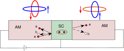
Figure 1: Schematic of the setup. An s-wave superconductor (SC) is sandwiched between two altermagnets (AMs) that are rotated by $90^{\circ}$ with respect to each other. Bias is applied from the left AM, maintaining the SC and the right AM grounded. An electron incident from the left AM onto SC can reflect either as an electron or as a hole, or transmit through SC and emerge onto the right AM as an electron or as a hole.

The Hamiltonian for an altermagnet is given by

$$H_{\vec{k}} = -2t_{0}(\cos{k_{x}a}+\cos{k_{y}a})\sigma_{0}$$ (1)

$$+2t_{J}(\cos{k_{x}a}-\cos{k_{y}a})\sigma_{z}-\mu,$$

where $t_{J}$ is the spin and direction dependent hopping which characterizes the altermagnetic phase, $t_{0}$ is the hopping, $a$ is the lattice spacing and $\sigma_{0},~{}\sigma_{z}$ are identity- and Pauli spin matrices. Altermagnets are classified depending upon whether $t_{J}>t_{0}$ or $t_{J}<t_{0}$, as strong- or weak- phase. We consider an AM-SC-AM junction arranged in such a way that the AM on the right is rotated by $90^{\circ}$ with respect to the AM on the left as shown in Fig. 1. We shall see that this helps in enhancing CAR. A bias is applied from the left AM, keeping the SC and the right AM grounded. We calculate the local conductivity $G_{LL}=dI_{L}/dV$ and the nonlocal conductivity $G_{RL}=dI_{R}/dV$, where $V$ is the bias, $I_{L}$ ($I_{R}$) is the current density in the left (right) AM, by Landauer-Büttiker approach Landauer (1957); Büttiker et al. (1985); Soori and Mukerjee (2017).

III Altermagnets in the strong phase

In this section, we consider the AMs to be in the strong phase by choosing $t_{0}=0$, $t_{J}>0$. The Hamiltonian for the AM on the left is obtained by expanding the Hamiltonian in eq. 1 around the band bottom. The band bottoms for the two spins are located at different points in the Brillouin zone. For the AM on the left, the band bottom for $\uparrow$ [$\downarrow$] -spin is at $(\pm\pi/a,0)$ [$(0,\pm\pi/a)$]. The Hamiltonian in the superconducting region mixes $\uparrow$ ($\downarrow$)-spin electron with $\downarrow$ ($\uparrow$)-spin hole. $\sigma_{z}$ commutes with the full Hamiltonian. Hence, we can work in the two sectors: (i) $\uparrow$-spin electron-$\downarrow$-spin hole [$\uparrow_{e}$, $\downarrow_{h}$], and (ii) $\downarrow$-spin electron-$\uparrow$-spin hole [$\downarrow_{e}$, $\uparrow_{h}$] separately.

III.1 ($\uparrow_{e}$, $\downarrow_{h}$) sector

In the sector (i), the Hamiltonian can be written as $\sum_{\vec{k}}\Psi_{\vec{k}}^{\dagger}H_{\vec{k}}\Psi_{\vec{k}}$, where $\Psi_{\vec{k}}=[c_{\uparrow,k},c^{\dagger}_{\downarrow,-k}]^{T}$ and

$$H_{\vec{k}} = [t_{J}((k_{x}a\pm\pi)^{2}+k_{y}^{2}a^{2})-\mu]\frac{\tau_{z}+\tau_{0}}{2}$$

$$+[t_{J}(k_{x}^{2}a^{2}+(k_{y}a\pm\pi)^{2})-\mu]\frac{\tau_{z}-\tau_{0}}{2},~{}~{}{\rm for}~{}~{}x<0$$

$$= \Big{[}\frac{\hbar^{2}~{}(k_{x}^{2}+k_{y}^{2})}{2~{}m}-\mu_{s}\Big{]}\tau_{z}+\Delta~{}\tau_{x},~{}~{}~{}{\rm for}~{}~{}0<x<L$$

$$= [t_{J}((k_{x}a\pm\pi)^{2}+k_{y}^{2}a^{2})-\mu]\frac{\tau_{z}-\tau_{0}}{2}$$

$$+[t_{J}(k_{x}^{2}a^{2}+(k_{y}a\pm\pi)^{2})-\mu]\frac{\tau_{z}+\tau_{0}}{2},~{}~{}{\rm for}~{}~{}x>L,$$

where $\tau_{j}$, for $j=0,x,z$ are the Pauli spin matrices acting on the particle-hole sector, $\Delta$ is the superconducting gap, and $c_{\vec{k},\sigma}$ annihilates an electron with wave vector $k$ and spin $\sigma$.

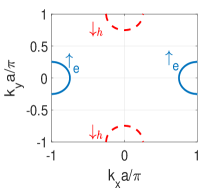
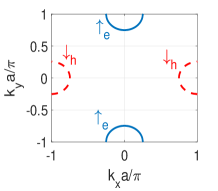
Figure 2: Schematic of the Fermi surfaces of altermagnets (AM) on the left and the right in the strong phase. Blue solid line shows $\uparrow_{e}$ and red dashed line shows $\downarrow_{h}$.

Four processes can occur when an electron is incident on the AM-SC-AM junction from the left AM. The electron with same spin can get reflected [electron reflection (ER)] or a hole with opposite spin can get reflected [Andreev reflection (AR)] Blonder et al. (1982) or an electron with same spin can transmit to the other AM [electron tunneling (ET)] or a hole with opposite spin can transmit to the other AM [crossed Andreev reflection (CAR)] Chtchelkatchev (2003); Beckmann et al. (2004). Conservation of probability current density along $x$-direction results in a competition among the four processes. Suppression of any one of them is balanced by enhancement in other processes. Since the system is translationally invariant along $y$-direction, matching and mismatching of $k_{y}$ in the dispersion relations on different sides determines which of the above phenomena is most likely to occur.

In this sector, $k_{y}$ for the up-spin electron on the left AM region matches with $k_{y}$ for the down-spin hole on the right AM side as can be seen in Fig. 2. So the hole gets transmitted to the right AM creating a Cooper pair in the SC and resulting in CAR. But $k_{y}$ for up-spin electron on the left AM region does not match with $k_{y}$ for up-spin electrons on the right AM region, thereby not allowing ET.

If on the right side the crystallographic orientation of the AM is same as that on the left side, then for $k_{y}$ of incident up-spin electrons, and that of down-spin hole on the right AM do not match, which means CAR is not possible. But $k_{y}$ values for the up-spin electrons on the left and the right AM regions match, resulting ET. Therefore, we notice that if we take two strong AMs whose crystallographic orientations are the same on the two sides of a SC, CAR does not occur. When the two AMs are oriented at $90^{\circ}$ to each other, CAR happens, but not ET.

The eigenstates in AM regions are either purely electron-like or purely hole-like. The energy eigenvalues in the left altermagnet for $\uparrow_{e}$ and $\downarrow_{h}$ are $E_{e,\uparrow}=t_{J}[(k_{ex}a-\pi)^{2}+k_{ey}^{2}a^{2}]-\mu$ and $E_{h,\downarrow}=-t_{J}[k_{hx}^{2}a^{2}+(k_{hy}a-\pi)^{2}]+\mu$ respectively. The eigenvectors for $\uparrow_{e}$ and $\downarrow_{h}$ are $[1,0]^{T}$ and $[0,1]^{T}$ respectively. The eigenenergies in the right AM are $E_{e,\uparrow}=t_{J}[k_{ex}^{2}a^{2}+(k_{ey}a\pm\pi)^{2}]-\mu$ and $E_{h,\downarrow}=-t_{J}[(k_{hx}a\pm\pi)^{2}+k_{hy}^{2}a^{2}]+\mu$.

In the SC region, the dispersion is $E=\pm\sqrt{[{\hbar^{2}}(q_{x}^{2}+q_{y}^{2})/2m-\mu_{s}]^{2}+\Delta^{2}}$. The eigenstates are Bogoliubov–de Gennes (BdG) quasiparticles, which have both the components: electron and hole. In the SC region, when the bias is within the superconducting energy gap, the BdG states are evanescent modes and are equally electron-like and hole-like. The eigenspinors are $[u_{j},\Delta]^{T}$, where

$$u_{j} =E+\frac{\hbar^{2}}{2m}(q_{xj}^{2}+q_{y}^{2})-\mu,$$

$$q_{x1} =\sqrt{\frac{2m}{\hbar^{2}}[\mu+\sqrt{E^{2}-\Delta^{2}}]-q_{y}^{2}},$$

$$q_{x2} =-\sqrt{\frac{2m}{\hbar^{2}}[\mu+\sqrt{E^{2}-\Delta^{2}}]-q_{y}^{2}},$$

$$q_{x3} =+\sqrt{\frac{2m}{\hbar^{2}}[\mu-\sqrt{E^{2}-\Delta^{2}}]-q_{y}^{2}},$$

$$q_{x4} =-\sqrt{\frac{2m}{\hbar^{2}}[\mu-\sqrt{E^{2}-\Delta^{2}}]-q_{y}^{2}},$$ (3)

where j takes value from 1 to 4.

An electron incident on the AM-SC interface from the left, results in four processes which can happen as said above. The wave function corresponding to this in different regions has the form $\psi~{}e^{ik_{ey}~{}y}$, where $\psi$ is given by

$$\psi = e^{ik_{exr}x}\begin{bmatrix}1\\ 0\\ \end{bmatrix}+r_{\uparrow_{e}}e^{i~{}k_{exl}x}\begin{bmatrix}1\\ 0\\ \end{bmatrix}$$ (4)

$$+r_{\downarrow_{h}}e^{-i~{}k_{hx}x}\begin{bmatrix}0\\ 1\\ \end{bmatrix},~{}~{}~{}{\rm for}~{}~{}x<0$$

$$= \sum_{j=1}^{4}B_{j}e^{iq_{xj}x}\begin{bmatrix}u_{j}\\ \Delta\\ \end{bmatrix},~{}~{}~{}~{}~{}~{}~{}{\rm for}~{}~{}0<x<L$$

$$= t_{\uparrow_{e}}e^{ik^{\prime}_{ex}x}\begin{bmatrix}1\\ 0\\ \end{bmatrix}+t_{\downarrow_{h}}e^{-ik^{\prime}_{hx\downarrow}x}\begin{bmatrix}0\\ 1\\ \end{bmatrix},~{}~{}{\rm for}~{}~{}x>L$$

where $r_{\uparrow_{e}},r_{\downarrow_{h}},t_{\uparrow_{e}}$ and $t_{\downarrow_{h}}$ are the coefficients for the processes: ER, AR, ET and CAR respectively. Here, $k_{exr}=\pi/a+k_{e}\cos{\theta}$, and $k_{exl}=\pi/a-k_{e}\cos{\theta}$ denote the wave vector of right moving electron and left moving electron respectively, $k_{hx}=\sqrt{k_{h}^{2}-(k_{ey}-\pi~{}{\rm sign}(\theta)/a)^{2}}$ is the wave vector of hole associated with Andreev reflected hole, $k^{\prime}_{ex}=\sqrt{k_{e}^{2}-(k_{ey}-\pi~{}{\rm sign}(\theta)/a)^{2}}$, $k^{\prime}_{hx\downarrow}=\pi/a-\sqrt{(k_{h}^{2}-k_{ey}^{2})}$ are the wave vectors of electron and hole which are associated with ET and CAR respectively, where $k_{e}a=\sqrt{{(\mu+E)}/{t_{J}}}$ and $k_{h}a=\sqrt{{(\mu-E)}/{t_{J}}}$. Due to the translational invariance along y direction, we have $q_{y}=k_{ey}=k_{e}\sin{\theta}$. Here, we choose the parameters so that $k_{hx}$ and $k^{\prime}_{ex}$ are imaginary. This means that AR and ET are absent. $k_{hx}$ and $k^{\prime}_{ex}$ have a positive imaginary part.

Now, to determine the scattering coefficients, boundary conditions are needed. These can be determined by demanding probability current density along $x$-direction. The probability current density along $x$ direction on the left AM is $J^{P}_{L,AM}=2t_{J}a^{2}[{\rm Im}(\psi^{{\dagger}}\tau_{z}\partial_{x}\psi)-\pi\psi^{{\dagger}}(\tau_{z}+\tau_{0})\psi/2a]/\hbar$, its counterpart on SC is $J^{P}_{SC}=~{}\hbar{\rm Im}[\psi^{{\dagger}}\tau_{z}\partial_{x}\psi]/m$ and the probability current density along $x$ direction on the right AM is $J^{P}_{R,AM}=2t_{J}a^{2}[{\rm Im}(\psi^{{\dagger}}\tau_{z}\partial_{x}\psi)-\pi\psi^{{\dagger}}(\tau_{z}-\tau_{0})\psi/2a]/\hbar$. From the most general boundary conditions possible, we choose the following:

$$\psi(0^{-}) = ~{}\psi(0^{+}),~{}~{}$$

$$\psi(L^{-}) = ~{}\psi(L^{+}),~{}~{}$$

$$\big{(}\frac{\hbar^{2}}{2~{}m~{}a^{2}~{}t_{J}}\partial_{x}\psi-q_{0}\psi\big{)}_{0^{+}} = \begin{pmatrix}\partial_{x}\psi_{e}-i\frac{\pi}{a}\psi_{e}\\ \partial_{x}\psi_{h}\end{pmatrix}_{0^{-}}~{}~{}$$

$$\big{(}\frac{\hbar^{2}}{2~{}m~{}a^{2}~{}t_{J}}\partial_{x}\psi+q_{0}\psi\big{)}_{L^{-}} = \begin{pmatrix}\partial_{x}\psi_{e}\\ \partial_{x}\psi_{h}-i\frac{\pi}{a}\psi_{h}\end{pmatrix}_{L^{+}}$$ (5)

where $\psi=[\psi_{e},~{}\psi_{h}]^{T}$. The parameter $q_{0}$ used in the boundary conditions quantifies the strength of the delta-function barrier at the interface Soori (2023). Using these boundary conditions on the wave function having the form in eq. (4), the scattering coefficients can be determined.

Charge density is given by $\rho_{c}=\psi^{{\dagger}}\tau_{z}\psi$. Charge density does not commute with the Hamiltonian in the SC region though it commutes with the Hamiltonian’s in the AMs. So, we calculate the currents densities on the two AMs. By using the continuity equation we find charge current density on the left and the right AMs. The expressions for the charge current densities on the left and right AMs upon substituting the form of the wavefunction, are given by

$$I_{L,\uparrow_{e},\downarrow_{h}} = \frac{2et_{J}}{\hbar}[k_{e}\cos{\theta}(1-|r_{\uparrow_{e}}|^{2})$$

$$I_{R,\uparrow_{e},\downarrow_{h}} = \frac{2et_{J}}{\hbar}[(k^{\prime}_{hx\downarrow}-\pi/a)|t_{\downarrow_{h}}|^{2}]$$ (6)

III.2 ($\downarrow_{e},\uparrow_{h}$) sector

In this sector, the calculation of currents can be done in a way similar to that followed in the previous section. For completeness, below we mention the Hamiltonian, boundary conditions, the scattering eigenfunction and the charge current density. The Hamiltonian for this sector is given by $\sum_{\vec{k}}\Psi_{\vec{k}}^{\dagger}H_{\vec{k}}\Psi_{\vec{k}}$, where $\Psi_{\vec{k}}=[c_{\downarrow,k},-c^{\dagger}_{\uparrow,-k}]^{T}$ and

$$\begin{split}H_{\vec{k}}&=[t_{J}(k_{x}^{2}a^{2}+(k_{y}a\pm\pi)^{2})-\mu]\frac{\tau_{z}+\tau_{0}}{2}\\ &+[t_{J}((k_{x}a\pm\pi)^{2}+k_{y}^{2}a^{2})-\mu]\frac{\tau_{z}-\tau_{0}}{2},~{}~{}{\rm~{}for}~{}~{}x<0\\ &=\Big{[}\frac{\hbar^{2}~{}(k_{x}^{2}+k_{y}^{2})}{2~{}m}-\mu_{s}\Big{]}\tau_{z}+\Delta~{}\tau_{x},~{}~{}~{}~{}~{}~{}~{}~{}{\rm for}~{}~{}0<x<L\\ &=[t_{J}((k_{x}a\pm\pi)^{2}+k_{y}^{2}a^{2})-\mu]\frac{\tau_{z}+\tau_{0}}{2}\\ &+[t_{J}(k_{x}^{2}a^{2}+(k_{y}a\pm\pi)^{2})-\mu]\frac{\tau_{z}-\tau_{0}}{2},~{}~{}{\rm for}~{}~{}x>L\end{split}$$

The wave function corresponding to an electron incident from the left AM onto the interface at energy $E$ and angle of incidence $\theta$ has the form $\psi~{}e^{ik_{ey}y}$, where $\psi$ is

$$\psi = e^{ik_{ex}x}\begin{bmatrix}1\\ 0\\ \end{bmatrix}+r_{\downarrow_{e}}e^{-ik_{ex}x}\begin{bmatrix}1\\ 0\\ \end{bmatrix}+r_{\uparrow_{h}}e^{ik_{hx}x}\begin{bmatrix}0\\ 1\\ \end{bmatrix},$$ (7)

$$~{}~{}~{}~{}~{}~{}{\rm for}~{}~{}x<0$$

$$= \sum_{j=1}^{4}B_{j}e^{iq_{xj}x}\begin{bmatrix}u_{j}\\ \Delta\\ \end{bmatrix},~{}~{}~{}~{}~{}~{}~{}{\rm~{}for}~{}~{}0<x<L$$

$$= t_{\downarrow_{e}}e^{ik^{\prime}_{ex}x}\begin{bmatrix}1\\ 0\\ \end{bmatrix}+t_{\uparrow_{h}}e^{ik^{\prime}_{hx\uparrow}x}\begin{bmatrix}0\\ 1\\ \end{bmatrix},~{}~{}~{}{\rm for}~{}~{}x>L$$

Here, $k_{ex}=k_{e}\cos{\theta}$ denotes the wave vector of right moving electron and $k_{hx}=\pi/a-\sqrt{k_{h}^{2}-k_{ey}^{2}}$ denotes the wave vector of hole in the region $x<0$ and $k_{ey}=\pi{\rm sign}(\theta)/a-k_{e}\sin{\theta}$ whereas $k^{\prime}_{ex}=\pi/a+\sqrt{k_{e}^{2}-k_{ey}^{2}}$, $k^{\prime}_{hx\uparrow}=-\sqrt{k_{h}^{2}-(k_{ey}-\pi~{}{\rm sign}(\theta)/a)^{2}}$ stand for the wave vector of electron and hole in the right AM ( $k_{e}a=\sqrt{{(\mu+E)}/{t_{J}}}$ and $k_{h}a=\sqrt{{(\mu-E)}/{t_{J}}}$. $\Im(k_{hx})<0$ and $\Im(k^{\prime}_{ex})>0$. The boundary conditions are

$$\psi(0^{-}) = ~{}\psi(0^{+}),~{}~{}$$

$$\begin{pmatrix}\partial_{x}\psi_{e}\\ \partial_{x}\psi_{h}-i\frac{\pi}{a}\psi_{h}\end{pmatrix}_{0^{-}} = \big{(}\frac{\hbar^{2}}{2~{}m~{}a^{2}~{}t_{J}}\partial_{x}\psi-q_{0}\psi\big{)}_{0^{+}}~{}~{}$$

$$\psi(L^{-}) = ~{}\psi(L^{+}),~{}~{}$$

$$\big{(}\frac{\hbar^{2}}{2~{}m~{}a^{2}~{}t_{J}}\partial_{x}\psi+q_{0}\psi\big{)}_{L^{-}} = \begin{pmatrix}\partial_{x}\psi_{e}-i\frac{\pi}{a}\psi_{e}\\ \partial_{x}\psi_{h}\end{pmatrix}_{L^{+}},$$ (8)

where $\psi=[\psi_{e},\psi_{h}]^{T}$

Charge current densities in on the left and right AM are given by

$$I_{L,\downarrow e,\uparrow h} = \frac{2~{}e~{}t_{J}}{\hbar}[k_{ex}~{}(1-|r_{\downarrow_{e}}|^{2})]$$

$$I_{R,\downarrow e,\uparrow h} = \frac{2~{}e~{}t_{J}}{\hbar}[k^{\prime}_{hx\uparrow}|t_{\uparrow_{h}}|^{2}]$$

III.3 Conductivity

The total current densities on the two AMs are $I_{L}=I_{L,\uparrow e,\downarrow h}+I_{L,\downarrow e,\uparrow h}$ and $I_{R}=I_{R,\uparrow e,\downarrow h}+I_{R,\downarrow e,\uparrow h}$. The differential conductivities on the two sides under a bias $V$ from left AM are given by

$$G_{LL} = \frac{e^{2}}{2\pi h}~{}k_{e}\Bigg{[}\int_{-\pi/2}^{\pi/2}(1-|r_{\uparrow_{e}}|^{2})\cos\theta\,d\theta$$

$$+\int_{-\pi/2}^{\pi/2}(1-|r_{\downarrow_{e}}|^{2})~{}\cos\theta\,d\theta\Bigg{]}$$

$$G_{RL} = \frac{e^{2}}{2\pi h}\Bigg{[}\int_{-\theta_{c}}^{\theta_{c}}(k^{\prime}_{hx\downarrow}-\pi/a)|t_{\downarrow_{h}}|^{2}d\theta+$$ (10)

$$\int_{-\theta_{c}}^{\theta_{c}}k^{\prime}_{hx\uparrow}|t_{\uparrow_{h}}|^{2}d\theta\Bigg{]},$$

where $\theta_{c}=\sin^{-1}[{\rm min}(k_{h}/k_{e},1)]$. Here, $G_{LL}$ is called the local conductivity and $G_{RL}$ the nonlocal conductivity.

III.4 Results and Analysis

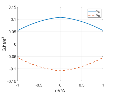
Figure 3: Local conductivity (blue line) and non-local conductivity (red dashed line) versus bias for $q_{0}=0$, $L=10.28a$, $m=\hbar^{2}/(a^{2}t_{J})$, $\mu=0.2t_{J}$, $\Delta=0.1t_{J}$ and $\mu_{s}=2t_{J}$ is shown

The local and nonlocal conductivities are numerically calculated following the procedure sketched in the previous subsections and plotted versus bias in Fig. 3 for the choice of parameters: $q_{0}=0$, $L=10.28~{}a$, $m=\hbar^{2}/(a^{2}t_{J})$, $\mu=0.2t_{J}$, $\Delta=0.1t_{J}$ and $\mu_{s}=2t_{J}$. We find that the local and non-local conductivity are exactly equal in magnitude and opposite in sign. This is because, there are only two processes that occur- CAR and ER. And from probability current conservation, the probability currents are equal on the left and the right AM. But, the charge current due to ER is $e$ times the probability current whereas the charge current due to CAR is $-e$ times the probability current. This makes the charge currents on the two sides equal in magnitude and opposite in sign. The non-local conductivity shows a negative peak at zero energy. This is because for $E=0$, $k_{e}$ becomes exactly equal to $k_{h}$ i.e $k_{ey}$ for all the incident electrons having momentum $k_{e}$, matches with $k_{hy}$ for all the holes in the other AM having momentum $k_{h}$. So the conversion of electron to hole is maximum giving rise to maximum CAR. But when energy $E\neq 0$, there is a mismatch in the momentum values for $\uparrow_{e}$ and $\downarrow_{h}$ resulting in lower conductivity. The non-local conductivity here is predominantly due to the up-spin electron incidence. The contribution to conductivities from the incident down spin electrons is $10^{-9}$ times the contribution from incident up spin electrons. The reason behind this is that for down-spin electron incidence $k_{ey}$ value is very large (near $\pi$) in comparison with $k_{ey}$ value for up-spin electron incidence (near $k_{ey}=0$). This results in a much smaller decay length for the evanescent modes in the SC region for the incident down spin electrons compared to that for the incident up spin electrons.

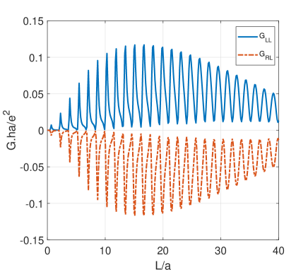
Figure 4: Local (solid blue line) and non-local (dash-dotted red line) conductivity versus the length of SC region are shown for $q_{0}=0$, $eV=0$, $m=\hbar^{2}/(a^{2}t_{J})$, $\mu=0.2t_{J}$, $\Delta=0.1t_{J}$ and $\mu_{s}=2t_{J}$.

Now, keeping all the parameters the same and fixing the bias to be at zero, we plot the conductivities versus length of the SC region in Fig. 4. The conductivities show oscillations due to Fabry-Pérot interference Soori et al. (2012); Liang et al. (2001); Soori (2019); Sahu and Soori (2023) in the superconducting region. Within the SC gap, the wave numbers in the SC region are not purely real. The real part of the wave numbers is responsible for the Fabry-Pérot interference. The Fabry-Pérot interference condition is $\Delta L=\pi/k$, where $\Delta L$ is the separation between the consecutive peaks and $k$ is the real part of the wave number of the interfering mode in the SC. Here, we take the $k$ for the normal incidence since the dominant contribution to the nonlocal transport is due to the electrons incident normal to the interface. The value of $\Delta L$ calculated from this condition is 1.5695a in comparison to 1.6053a that is observed in the results in Fig. 4. Further, the peak value of the magnitude of non-local conductivity first increases with length, reaches a maximum value up to the order of $10^{-1}$ for superconducting length nearly equal to $15a$ and then gradually decreases. The global peak in the magnitude of nonlocal conductivity is due to maximum CAR which happens when the length of the SC is approximately inverse of the imaginary part of the wave number in the SC region which is $20a$. The nonlocal conductivity is always negative for altermagnets in strong phase chosen with appropriate crystallographic orientation signalling dominant CAR in comparison with ET. This is in contrast to other schemes of enhancement of CAR wherein the contribution to nonlocal conductivity from ET is typically nonzero.

IV Altermagnets in weak phase

In this section we choose the AMs to be in the weak phase by choosing $t_{0}>t_{J}\geq 0$. Unlike in the strong phase, the band bottoms for both the spins are located at $k_{x}=k_{y}=0$. But the Fermi surfaces do not overlap, rather they intersect each other due to their anisotropic behavior. As a result, for a given spin, all the $k_{y}$ values for the electrons of AMs on either sides of the SC do not match. However, the $k_{y}$ values for electrons of spin $\sigma$ on one side match with $k_{y}$ values for holes of spin $\bar{\sigma}$ to a much larger extent. This can be seen from Fig. 5. Therefore, CAR is favored over ET.

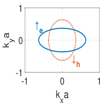
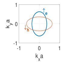
Figure 5: Fermi surfaces of altermagnets (AM) on the left and the right in weak phase, blue solid line showing $\uparrow_{e}$ and red dotted line shows $\downarrow_{h}$ for $t_{J}=0.5t_{0}$ and $\mu=0.2t_{0}$

IV.1 ($\uparrow_{e},\downarrow_{h}$) sector

In this sector, the Hamiltonian can be written similar to ($\uparrow_{e}$, $\downarrow_{h}$) case in strong phase. The difference is that now the dispersion is expanded around $k_{x}=0,k_{y}=0$ as the band bottom lies there. The Hamiltonian is:

$$\begin{split}H_{\vec{k}}&=[(t_{0}-t_{J})~{}k_{x}^{2}a^{2}+(t_{0}+t_{J})~{}k_{y}^{2}a^{2}-\mu]\frac{\tau_{z}+\tau_{0}}{2}\\ &+[(t_{0}+t_{J})~{}k_{x}^{2}a^{2}+(t_{0}-t_{J})~{}k_{y}^{2}a^{2})-\mu]\frac{\tau_{z}-\tau_{0}}{2},~{}~{}~{}{\rm for}~{}~{}x<0\\ &=\Big{[}\frac{\hbar^{2}~{}(k_{x}^{2}+k_{y}^{2})}{2~{}m}-\mu_{s}\Big{]}\tau_{z}+\Delta~{}\tau_{x},~{}~{}~{}~{}{\rm for}~{}~{}~{}0<x<L\\ &=[(t_{0}+t_{J})~{}k_{x}^{2}a^{2}+(t_{0}-t_{J})~{}k_{y}^{2}a^{2}-\mu]\frac{\tau_{z}+\tau_{0}}{2}\\ &+[(t_{0}-t_{J})~{}k_{x}^{2}a^{2}+(t_{0}+t_{J})~{}k_{y}^{2}a^{2})-\mu]\frac{\tau_{z}-\tau_{0}}{2},~{}~{}~{}{\rm for}~{}~{}x>L\\ \end{split}$$

In Fig. 5, the Fermi surfaces for AMs on the two sides are shown. The wave function corresponding to the Hamiltonian in different regions possesses the form $\psi~{}e^{ik_{ey}y}$, where $\psi$ is given by

$$\psi = e^{ik_{ex\uparrow}x}\begin{bmatrix}1\\ 0\\ \end{bmatrix}+r_{\uparrow_{e}}e^{-ik_{ex\uparrow}x}\begin{bmatrix}1\\ 0\\ \end{bmatrix}+r_{\downarrow_{h}}e^{ik_{hx\downarrow}x}\begin{bmatrix}0\\ 1\\ \end{bmatrix},$$

$$~{}~{}~{}~{}{\rm~{}for~{}}x<0$$

$$= \sum_{j=1}^{4}B_{j}e^{iq_{xj}x}\begin{bmatrix}u_{j}\\ \Delta\\ \end{bmatrix},~{}~{}~{}~{}~{}~{}~{}~{}{\rm for~{}~{}}0<x<L$$

$$= t_{\uparrow_{e}}e^{ik^{\prime}_{ex\uparrow}x}\begin{bmatrix}1\\ 0\\ \end{bmatrix}+t_{\downarrow_{h}}e^{ik^{\prime}_{hx\downarrow}x}\begin{bmatrix}0\\ 1\\ \end{bmatrix},~{}~{}~{}~{}~{}~{}{\rm for}~{}~{}~{}~{}~{}x>L$$

and $r_{\uparrow_{e}},r_{\downarrow_{h}},t_{\uparrow_{e}}$ and $t_{\downarrow_{h}}$ are the scattering coefficients for ER, AR, ET and CAR respectively. Here, $k_{ex\uparrow}a=\sqrt{(E+\mu)/(t_{0}-t_{J})}\cos{\theta}$ is the wave vector associated with right moving electron, $k_{ey}a=\sqrt{(E+\mu)/(t_{0}+t_{J})}\sin{\theta}$ is the component of wave vector of electron along $y$-direction. $k_{hx\downarrow}a=\sqrt{\big{[}(\mu-E)-(t_{0}-t_{J})~{}k_{ey}^{2}a^{2}\big{]}/(t_{0}+t_{J})}$ is the wave vector associated with reflected hole in left AM whereas $k^{\prime}_{ex\uparrow}a=\sqrt{\big{[}(\mu+E)-(t_{0}-t_{J})~{}k_{ey}^{2}a^{2}\big{]}/(t_{0}+t_{J})}$ and $k^{\prime}_{hx\downarrow}a=-\sqrt{\big{[}(\mu-E)-(t_{0}+t_{J})~{}k_{ey}^{2}a^{2}\big{]}/(t_{0}-t_{J})}$ stand for the wave vectors for the transmitted electron and transmitted hole respectively. Whenever any of these wave numbers turn out to be complex, the square root is taken so that the wave decays to zero at $x\to\pm\infty$.

The probability current density along $x$ direction on the left AM is $J^{P}_{L,AM}=2(t_{0}-t_{J})a^{2}[{\rm Im}(\psi^{{\dagger}}(\tau_{z}+\tau_{0})\partial_{x}\psi)/2]/\hbar-2(t_{0}+t_{J})a^{2}[{\rm Im}(\psi^{{\dagger}}(\tau_{z}-\tau_{0})\partial_{x}\psi)/2]/\hbar$, its counterpart on SC is $J^{P}_{SC}=~{}\hbar a^{2}{\rm Im}[\psi^{{\dagger}}\tau_{z}\partial_{x}\psi]/m$ whereas the probability current on the right AM is $J^{P}_{R,AM}=2(t_{0}+t_{J})a^{2}[{\rm Im}(\psi^{{\dagger}}(\tau_{z}+\tau_{0})\partial_{x}\psi)/2]/\hbar-2(t_{0}-t_{J})a^{2}[{\rm Im}(\psi^{{\dagger}}(\tau_{z}-\tau_{0})\partial_{x}\psi)/2]/\hbar$. From probability current conservation on the two sides we can find the boundary conditions which will ultimately help us in determining the scattering coefficients. We choose the following boundary conditions:

$$\psi(0^{-}) = ~{}\psi(0^{+}),~{}~{}$$

$$\partial_{x}\psi|_{0^{-}} = \begin{pmatrix}\frac{\hbar^{2}}{2ma^{2}(t_{0}-t_{J})}\partial_{x}\psi_{e}-q_{0}\psi_{e}\\ \frac{\hbar^{2}}{2ma^{2}(t_{0}+t_{J})}\partial_{x}\psi_{h}-q_{0}\psi_{h}\end{pmatrix}_{0^{+}}~{}~{}$$

$$\psi(L^{+}) = ~{}\psi(L^{-}),~{}~{}$$

$$\partial_{x}\psi|_{L^{+}} = \begin{pmatrix}\frac{\hbar^{2}}{2ma^{2}(t_{0}+t_{J})}\partial_{x}\psi_{e}+q_{0}\psi_{e}\\ \frac{\hbar^{2}}{2ma^{2}(t_{0}-t_{J})}\partial_{x}\psi_{h}+q_{0}\psi_{h}\end{pmatrix}_{L^{-}}$$ (12)

Charge current density in the left and right AM are given by the following expressions:

$$I_{L,\uparrow_{e},\downarrow_{h}} = \frac{2e}{\hbar}[(t_{0}-t_{J})k_{e}\cos{\theta}(1-|r_{\uparrow_{e}}|^{2})$$

$$+(t_{0}+t_{J})\Re(k_{hx\downarrow})|r_{\downarrow_{h}}|^{2}]$$

$$I_{R,\uparrow_{e},\downarrow_{h}} = \frac{2e}{\hbar}[(t_{0}+t_{J})\Re(k^{\prime}_{ex\uparrow})|t_{\uparrow_{e}}|^{2}$$ (13)

$$-(t_{0}-t_{J})\Re(k^{\prime}_{hx\downarrow})|t_{\downarrow_{h}}|^{2}]$$

IV.2 ($\downarrow_{e},\uparrow_{h}$) sector

We use a similar method to find the current density in this sector. So we start with the Hamiltonian:

$$\begin{split}H_{\vec{k}}&=[(t_{0}+t_{J})~{}k_{x}^{2}a^{2}+(t_{0}-t_{J})~{}k_{y}^{2}a^{2}-\mu]\frac{\tau_{z}+\tau_{0}}{2}\\ &+[(t_{0}-t_{J})~{}k_{x}^{2}a^{2}+(t_{0}+t_{J})~{}k_{y}^{2}a^{2})-\mu]\frac{\tau_{z}-\tau_{0}}{2},~{}~{}~{}{\rm for}~{}~{}x<0\\ &=\Big{[}\frac{\hbar^{2}~{}(k_{x}^{2}+k_{y}^{2})}{2~{}m}-\mu_{s}\Big{]}\tau_{z}+\Delta~{}\tau_{x},~{}~{}~{}~{}~{}~{}~{}~{}~{}{\rm for}~{}~{}~{}0<x<L\\ &=[(t_{0}-t_{J})~{}k_{x}^{2}a^{2}+(t_{0}+t_{J})~{}k_{y}^{2}a^{2}-\mu]\frac{\tau_{z}+\tau_{0}}{2}\\ &+[(t_{0}+t_{J})~{}k_{x}^{2}a^{2}+(t_{0}-t_{J})~{}k_{y}^{2}a^{2})-\mu]\frac{\tau_{z}-\tau_{0}}{2},~{}~{}~{}{\rm for}~{}~{}x>L\\ \end{split}$$

The wave function for the system has the form $\psi~{}e^{ik_{ey}y}$ where

$$\psi = e^{ik_{ex\downarrow}x}\begin{bmatrix}1\\ 0\\ \end{bmatrix}+r_{\downarrow_{e}}e^{-ik_{ex\downarrow}x}\begin{bmatrix}1\\ 0\\ \end{bmatrix}+r_{\uparrow_{h}}e^{-ik_{hx\uparrow}x}\begin{bmatrix}0\\ 1\\ \end{bmatrix},$$ (14)

$$~{}~{}~{}~{}~{}~{}~{}~{}~{}~{}~{}~{}~{}~{}~{}~{}~{}~{}~{}~{}~{}~{}~{}~{}~{}~{}~{}~{}~{}~{}~{}~{}~{}~{}~{}~{}~{}~{}~{}~{}~{}~{}~{}~{}{\rm for}~{}~{}x<0$$

$$= \sum_{j=1}^{4}B_{j}e^{iq_{xj}x}\begin{bmatrix}u_{j}\\ \Delta\\ \end{bmatrix},~{}~{}~{}~{}~{}~{}~{}~{}~{}~{}~{}{\rm for}~{}~{}0<x<L$$

$$= t_{\downarrow_{e}}e^{ik^{\prime}_{ex\downarrow}x}\begin{bmatrix}0\\ 1\\ \end{bmatrix}+t_{\uparrow_{h}}e^{ik^{\prime}_{hx\uparrow}x}\begin{bmatrix}1\\ 0\\ \end{bmatrix},~{}~{}{\rm for}~{}~{}x>L,$$

and $k_{ex\downarrow}a=\sqrt{(E+\mu)/(t_{0}+t_{J})}~{}\cos{\theta}$,
$k_{ey}a=\sqrt{(E+\mu)/(t_{0}-t_{J})}~{}\sin{\theta}$,
$k_{hx\uparrow}a=\sqrt{\big{[}(\mu-E)-(t_{0}+t_{J})~{}k_{ey}^{2}a^{2}\big{]}/{(t_{0}-t_{J})}},\\ k^{\prime}_{ex\downarrow}a=\sqrt{[(E+\mu)-(t_{0}+t_{J})~{}k_{ey}^{2}a^{2}]/{(t_{0}-t_{J})}}$,
$k^{\prime}_{hx\uparrow}a=\sqrt{[(\mu-E)-(t_{0}-t_{J})~{}k_{ey}^{2}a^{2}]/{(t_{0}+t_{J})}}$.
All the above terms have the same meaning as mentioned in the previous subsection. The boundary conditions for this sector are given by

$$\psi(0^{-}) = ~{}\psi(0^{+}),~{}~{}$$

$$\partial_{x}\psi|_{0^{-}} = \begin{pmatrix}\frac{\hbar^{2}}{2ma^{2}(t_{0}+t_{J})}\partial_{x}\psi_{e}-q_{0}\psi_{e}\\ \frac{\hbar^{2}}{2ma^{2}(t_{0}-t_{J})}\partial_{x}\psi_{h}-q_{0}\psi_{h}\end{pmatrix}_{0^{+}}~{}~{}$$

$$\psi(L^{+}) = ~{}\psi(L^{-}),~{}~{}$$

$$\partial_{x}\psi|_{L^{+}} = \begin{pmatrix}\frac{\hbar^{2}}{2ma^{2}(t_{0}-t_{J})}\partial_{x}\psi_{e}+q_{0}\psi_{e}\\ \frac{\hbar^{2}}{2ma^{2}(t_{0}+t_{J})}\partial_{x}\psi_{h}+q_{0}\psi_{h}\end{pmatrix}_{L^{-}}$$ (15)

Charge current density in the left and right AM are given by the following expressions:

$$I_{L,\downarrow_{e},\uparrow_{h}} = \frac{2e}{\hbar}[(t_{0}+t_{J})k_{e}\cos{\theta}(1-|r_{\downarrow_{e}}|^{2})$$

$$+(t_{0}-t_{J})\Re(k_{hx\downarrow})|r_{\uparrow_{h}}|^{2}]$$

$$I_{R,\downarrow_{e},\uparrow_{h}} = \frac{2e}{\hbar}[(t_{0}-t_{J})\Re(k^{\prime}_{ex\downarrow})|t_{\downarrow_{e}}|^{2}$$ (16)

$$-(t_{0}+t_{J})\Re(k^{\prime}_{hx\uparrow})|t_{\uparrow_{h}}|^{2}]$$

IV.3 Conductivity

The total current densities on the two AMs are $I_{L}=I_{L,\uparrow e,\downarrow h}+I_{L,\downarrow e,\uparrow h}$ and $I_{R}=I_{R,\uparrow e,\downarrow h}+I_{R,\downarrow e,\uparrow h}$. The differential conductivities on the two sides under a bias $V$ from left AM are given by

$$G_{LL} = \frac{e^{2}}{2\pi h}\Bigg{[}\sqrt{\frac{t_{0}-t_{J}}{t_{0}+t_{J}}}\int_{-\pi/2}^{\pi/2}~{}k_{ex\uparrow}(1-|r_{\uparrow_{e}}|^{2})d\theta$$

$$+\sqrt{\frac{t_{0}+t_{J}}{t_{0}-t_{J}}}\int_{-\theta_{h\uparrow}}^{\theta_{h\uparrow}}k_{hx\downarrow}(|r_{\downarrow_{h}}|^{2})d\theta$$

$$+\sqrt{\frac{t_{0}+t_{J}}{t_{0}-t_{J}}}\int_{-\pi/2}^{\pi/2}~{}k_{ex\downarrow}(1-|r_{\downarrow_{e}}|^{2})d\theta$$

$$+\sqrt{\frac{t_{0}-t_{J}}{t_{0}+t_{J}}}\int_{-\theta_{h\downarrow}}^{\theta_{h\downarrow}}k_{hx\uparrow}(|r_{\uparrow_{h}}|^{2})d\theta\Bigg{]},$$

$${\rm where~{}~{}}$$

$$\theta_{h\uparrow}=\sin^{-1}\Bigg{[}{\rm min}\Big{[}\frac{(\mu-E)(t_{0}+t_{J})}{(\mu+E)(t_{0}-t_{J})},1\Big{]}\Bigg{]},$$

$$\theta_{h\downarrow}=\sin^{-1}\Bigg{[}{\rm min}\Big{[}\frac{(\mu-E)(t_{0}-t_{J})}{(\mu+E)(t_{0}+t_{J})},1\Big{]}\Bigg{]}.$$

$$G_{RL} = \frac{e^{2}}{2\pi h}\Bigg{[}\sqrt{\frac{t_{0}+t_{J}}{t_{0}-t_{J}}}\int_{-\pi/2}^{\pi/2}k^{\prime}_{ex\uparrow}(|t_{\uparrow_{e}}|^{2})d\theta$$ (18)

$$-\sqrt{\frac{t_{0}-t_{J}}{t_{0}+t_{J}}}\int_{-\theta_{h}}^{\theta_{h}}k^{\prime}_{hx\downarrow}(|t_{\downarrow_{h}}|^{2})d\theta$$

$$+\sqrt{\frac{t_{0}-t_{J}}{t_{0}+t_{J}}}\int_{-\theta_{e}}^{\theta_{e}}k^{\prime}_{ex\downarrow}(|t_{\downarrow_{e}}|^{2})d\theta$$

$$-\sqrt{\frac{t_{0}+t_{J}}{t_{0}-t_{J}}}\int_{-\theta_{h}}^{\theta_{h}}k^{\prime}_{hx\uparrow}(|t_{\uparrow_{h}}|^{2})d\theta\Bigg{]},$$

where $\theta_{e}=\sin^{-1}[\sqrt{(t_{0}-t_{J})/(t_{0}+t_{J})}]$ and $\theta_{h}=\sin^{-1}[{\rm min}\{(\mu-E)/(\mu+E),1\}]$.

IV.4 Results and Analysis

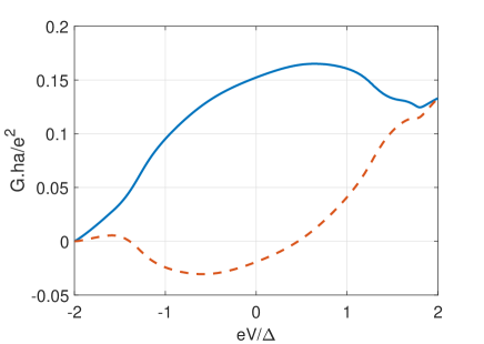
Figure 6: Local conductivity (blue line) and non-local conductivity (red dashed line) versus bias for $q_{0}=0$, $L=7a$,$t_{J}=0.8t_{0}$ $m=\hbar^{2}/(a^{2}t_{0})$, $\mu=0.2t_{0}$, $\Delta=0.1t_{0}$ and $\mu_{s}=2t_{0}$ is shown

In fig. 6, we plot the two conductivities versus bias and find that CAR dominates over ET for a certain range of bias within the SC gap. Because, within the superconducting gap, the electron to hole conversion has higher probability.

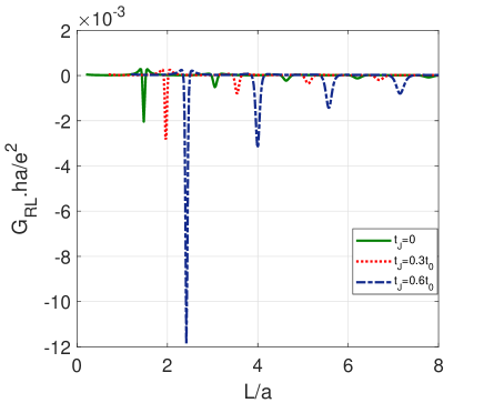
Figure 7: Non-local conductivity versus length of SC for $t_{J}=0$ (green solid line), $t_{J}=0.3t_{0}$ (red dotted-line), $t_{J}=0.6t_{0}$(blue dash-dot line), $E=0$, $q_{0}=10t_{0}$, $m=\hbar^{2}/(a^{2}t_{0})$, $\mu=0.2t_{0}$, $\Delta=0.1t_{0}$, $\mu_{s}=2t_{0}$. Red dotted and blue dash-dot curves are shifted by 0.5 and 1.0 units along $x$-axis respectively for clarity.

In fig.7, the variation of non-local conductivity with length for different values of $t_{J}$ is shown. $t_{J}=0$ corresponds to the absence of altermagnetic phase, and the leads behave as normal metal leads. We notice that when $t_{J}\neq 0$ the non-local conductivity is higher in magnitude as compared to when $t_{J}=0$. Thus, we find that AM helps to enhance CAR in comparison to a normal metal. The larger the value of $t_{J}$ within the range $0<t_{J}<t_{0}$, the larger is the non-local conductivity in magnitude. The non-local conductivity plot shows a negative peak for some definite values of length, and this peak is periodic in nature. The reason behind this is that the wave gets multiply reflected back-and-forth within the SC region and picks up a phase of $2\Re(q_{x})L$ in one round of back-and-forth reflection, where $q_{x}$ is the wave number in the SC region. According to the Fabry-Pérot interference condition, when this phase difference is integral multiple of $2\pi$, we get constructive interference resulting in peaks. The separation between two consecutive negative peaks can be calculated by $\Delta L={\pi}/{\Re(q_{x})}$. The value of $\Delta L$ calculated from this formula is $1.57a$ and the value observed in Fig. 7 is $\sim 1.58a$.

V Experimental relevance

Let us see how the parameters $t_{0}$ and $t_{J}$ used in the model are connected to real materials, taking the example of RuO₂. In RuO₂, the bandwidth and the spin splitting are of the same order of magnitude $\sim 1eV$ Papaj (2023); Šmejkal et al. (2022c). However, the SC gap in realistic materials like NbSe₂ is of the order of few $meV$ making the ratio of $\Delta/t_{0}\sim 10^{-3}$. The nonlocal conductivity is not negative for such a choice of parameters. To get negative nonlocal conductivity, $\Delta/t_{0}$ needs to be of the order of $0.1$ maintaining $t_{J}\gtrsim t_{0}$. So, altermagntic materials with $t_{0}\lesssim t_{J}\sim 10meV$ are desired to observe the effects we studied in this work.

VI Conclusion

We propose to employ the newly discovered altermagnets to enhance and detect crossed Andreev reflection across an s-wave superconductor. When the two AMs are rotated by $90^{\circ}$ with respect to each other, CAR can be enhanced significantly. We calculated the local and nonlocal conductivities for AM-SC-AM junctions. We find that when the altermagnets are in the strong phase, the nonlocal transport can be completely dominated by CAR with zero contribution from ET. On the other hand, when the AMs are in the weak phase, both ET and CAR contribute to the nonlocal conductivity. But, for certain choice of parameters, we can get larger contribution from CAR than from ET. The nonlocal conductivity shows extrema for certain values of the length of the SC which is rooted in Fabry-Pérot type interference. So, for certain specially chosen values of the length of the SC, the system exhibits enhanced CAR even in the weak phase of AM. Our results will be useful in development of superconducting devices based on the phenomenon of CAR such as Cooper pair splitters.