A multi-wavelength study of the hard and soft states of MAXI J1820+070 during its 2018 outburst

Abstract

We present a comprehensive multi-wavelength spectral analysis of the black hole X-ray binary MAXI J1820+070 during its 2018 outburst, utilizing AstroSat far UV, soft and hard X-ray data, along with (quasi-)simultaneous optical and X-ray data from Las Cumbres Observatory and NICER, respectively. In the soft state, we detect soft X-ray and UV/optical excess components over and above the intrinsic accretion disk emission ($kT_{\rm in}\sim 0.58$ keV) and a steep X-ray power-law component. The soft X-ray excess is consistent with a high-temperature blackbody ($kT\sim 0.79$ keV), while the UV/optical excess is described by UV emission lines and two low-temperature blackbody components ($kT\sim 3.87$ eV and $\sim 0.75$ eV). Employing continuum spectral fitting, we determine the black hole spin parameter ($a=0.77\pm 0.21$), using the jet inclination angle of $64^{\circ}\pm 5^{\circ}$ and a mass spanning $5-10M_{\sun}$. In the hard state, we observe a significantly enhanced optical/UV excess component, indicating a stronger reprocessed emission in the outer disk. Broad-band X-ray spectroscopy in the hard state reveals a two-component corona, each associated with its reflection component, in addition to the disk emission ($kT_{\rm in}\sim 0.19$ keV). The softer coronal component dominates the bolometric X-ray luminosity and produces broader relativistic reflection features, while the harder component gets reflected far from the inner disk, yielding narrow reflection features. Furthermore, our analysis in the hard state suggests a substantial truncation of the inner disk ($\gtrsim 51$ gravitational radii) and a high disk density ($\sim 10^{20}\ \rm cm^{-3}$).

1 Introduction

A low-mass X-ray binary (LMXB) containing a black hole (BH) is a binary stellar system in which the BH accretes matter from a low-mass companion star ($\lesssim 1M_{\sun}$) via the Roche-lobe overflow. Most of the Galactic BH-LMXBs are of transient nature, spending most of their lifetime in a faint quiescent state. This inactive period is sporadically interrupted by short outbursts (usually lasting for weeks to months), in which the accretion rate increases by several orders of magnitude. During an outburst, a BH-LMXB often evolves through a sequence of different X-ray spectral states: Hard State (HS), Soft State (SS) and Hard/Soft Intermediate state (HIMS/SIMS) (Belloni, 2010; Remillard & McClintock, 2006), displaying a ‘q’ shaped track in the hardness-intensity diagram (HID) (Homan et al., 2001; Homan & Belloni, 2005). These spectral states differ in their spectral and timing properties, and are possibly due to a change in the accretion geometry (Belloni & Motta, 2016).

A typical outburst of BH-LMXBs generally starts and ends in the HS. The HS X-ray spectrum is dominated by an optically thin component exhibiting roughly a power-law shape (with a photon index of $1.4<\Gamma<2.1$), from a few keV to several hundred keV, followed by an exponential cutoff (Remillard & McClintock, 2006). Although the accretion geometry of the HS is highly debated, this component is thought to arise due to the Compton up-scattering of soft seed photons by a hot optically thin electron cloud (‘corona’) located somewhere in the vicinity of the compact object (Sunyaev & Titarchuk, 1980; Done et al., 2007; Gilfanov, 2010; Banerjee et al., 2020). Additionally, there could be a weak contribution to the X-ray spectrum from an optically thick and geometrically thin accretion disk with low temperature, with a typical temperature of $\sim 0.2$ keV (Reis et al., 2009; Basak & Zdziarski, 2016; Zhang et al., 2020). The lower disk temperature generally suggests that the disk is truncated far from the innermost stable circular orbit (ISCO) (Zdziarski et al., 2021a; Done et al., 2007; Gilfanov, 2010) (however, for other scenarios, see Reis et al. 2010; Kara et al. 2019). After starting in the HS, a source usually transitions to the SS, and returns to the HS towards the end of the outburst. The SS spectrum is described primarily by a multi-temperature black-body component originating in the accretion disk (Shakura & Sunyaev, 1973), often accompanied by a weak and steep ($\Gamma\geq 2.1$) power-law tail extending out beyond 500 keV (Belloni & Motta, 2016). The black-body component typically peaks $\sim 1$ keV, and the disk, contrary to the HS case, reaches close to the ISCO radius (Done et al., 2007; Gilfanov, 2010). While evolving from the HS to SS (or SS to HS), a BH-LMXB goes through HIMS and SIMS (or SIMS and HIMS) successively. The soft thermal disk component becomes more dominant (accompanied by a decrease in power-law flux) in these intermediate states than the HS.

Apart from the hard Comptonized and soft thermal components, the X-ray spectrum of BH-LMXBs also exhibits reflection features, generated as a fraction of Compton up-scattered photons gets reprocessed in the inner accretion disk. These features mainly include a reflection hump around 20-40 keV, and an iron K$\alpha$ line around $6.4-6.97$ keV that are modified by special and general relativistic effects near the BH (Fabian et al., 1989; Fabian, 2005). Besides providing detailed information on the composition and ionization state of the disk, the relativistic X-ray reflection provides a way to determine the spin of the BH and also sheds light on the structure of the corona (García et al., 2013, 2014).

By contrast with this wealth of data in the X-ray band, the emission in the optical/UV band from these systems is poorly understood. It has been widely accepted that the reprocessing of X-rays in the outer accretion disk is the dominant source of optical/UV emission for BH-LMXBs in the SS (van Paradijs & McClintock, 1994). In the HS, the synchrotron emission from the jet can also contribute significantly in the optical/UV band (Russell et al., 2006). Although it is difficult to disentangle the effect of these two components from an individual optical/UV spectrum, theoretical models have predicted that the UV/optical luminosity ($L_{\rm optical/UV}$) is correlated differently with the X-ray luminosity if the emission process is irradiation heating ($L_{\rm optical/UV}\propto L_{X}^{0.5}$) or radiation from the jet ($L_{\rm optical/UV}\propto L_{X}^{0.7}$) (Gierliński et al., 2009). However, optical/infrared and X-ray (in 2-10 keV band) observations of a large sample of X-ray binaries in the hard state suggest that both the X-ray reprocessing in the disk and the jet emission show a slope close to 0.6 (holds over from B to K band) for BH-LMXBs (Russell et al., 2006). Besides, the intrinsic thermal emission (due to viscous heating) from the outer disk may also provide significant optical/UV photons in both states.

The transient LMXB MAXI J1820+070 was discovered with the Monitor of All-Sky X-ray Image (MAXI) on March 11 2018 (Kawamuro et al., 2018), and five days prior in the optical band with the All-Sky Automated Survey for SuperNovae (ASSAS-SN) project (Denisenko, 2018). Soon after its discovery, X-ray flux and optical G magnitude rose to $\sim 4$ Crab (Shidatsu et al., 2019) and $\sim 11.2$ (Torres et al., 2019), respectively, making it one of the brightest X-ray transients ever observed. The source remained bright and active for several months and underwent re-brightening episodes before fading into quiescence in February 2019 (Russell et al., 2019a). Thanks to its low Galactic interstellar absorption ($N_{\rm H}\sim 1.3\times 10^{21}\ \rm cm^{-2}$, HI4PI Collaboration et al. (2016)), and relatively nearby location ($2.96\pm 0.33$ kpc, Atri et al. (2020)), the source has been extensively monitored across several wavelengths: from radio (Trushkin et al., 2018; Bright et al., 2018) to infrared (Casella et al., 2018; Mandal et al., 2018) to optical (Baglio et al., 2018; Littlefield, 2018; Sako et al., 2018; Gandhi et al., 2018; Bahramian et al., 2018; Russell et al., 2019a) to X-rays (Uttley et al., 2018; Homan et al., 2018), producing a wealth of information about this accreting system.

The object was dynamically confirmed as a BH with a mass of $M=(5.95\pm 0.22)M_{\sun}/\rm sin^{3}(i_{b})$ ($i_{b}$: binary inclination angle) with a K-type companion star (Torres et al., 2020) of mass $0.49\pm 0.10M_{\sun}$ (Mikołajewska et al., 2022). The binary inclination angle was estimated as $66^{\circ}<i_{b}<81^{\circ}$ (Torres et al., 2020), although the jet inclination (which is generally assumed to be parallel to the BH spin axis) was found to be $64^{\circ}\pm 5^{\circ}$ (Wood et al., 2021). On the other hand, Buisson et al. (2019) found the same to be $30_{-5}^{+4}$ degree in their reflection analysis with NuSTAR data. However, the detection of X-ray dips confirms that the inclination of the outer disk is indeed high (Kajava et al., 2019).

The source went through all canonical states of a BH-LMXBs during the 2018 outburst, following roughly the typical ’q’ pattern on HID (Buisson et al., 2019; Chakraborty et al., 2020). It initially stayed in the HS over three months and transitioned to the SS in July 2018 (Homan et al., 2020). A compact jet was observed in the HS (Bright et al., 2018). Also, a strong radio flare associated with the launch of bipolar superluminal ejecta was detected at the beginning of the transition to the SS (Bright et al., 2020). The long-term optical and X-ray monitoring of the source during the outburst phase suggests that the jet contributed significantly to the optical emission in the HS state, while the outer disk emission through irradiation provides the dominant optical flux in the intermediate states, and SS (Shidatsu et al., 2019).

The initial spectral analysis of the HS data implied that two Comptonization components are required to offer a satisfactory fit to the data, and the disk extends close to the ISCO radius (Buisson et al., 2019; Chakraborty et al., 2020). The inclination angle was reported low ($\sim 30$ degree), and iron abundance ($\sim 5$ times solar abundance) was found to be high in these studies. The spectro-timing analysis of Kara et al. (2019) supported their claim related to the extent of the disk. Kara et al. (2019) found out that the corona reduced in spatial extent as the source moves toward the SS from the HS, while the inner disk stays stable roughly at $\sim 2R_{g}$. On the contrary, the disk was observed to be truncated far from the source in the HS in the spectral analysis of Zdziarski et al. (2021a, b, 2022b) with a two-component corona. Besides, the spectral-timing analysis of De Marco et al. (2021) and Axelsson & Veledina (2021) validate the above observation. Interestingly, the inclination in these works (Zdziarski et al., 2021a, 2022b) was found to be close to the jet inclination angle, and the iron abundance was roughly solar. Finally, the SS observations of this source show an excess emission component in the X-ray spectrum which was proposed to originate from the plunging region (Fabian et al., 2020). Fabian et al. (2020) also found (using NICER SS data) that the mass of the BH is $\sim 5-10M_{\sun}$ and the spin lies in the range of 0.5 to -0.5 (for an inclination in the range of $30^{\circ}-40^{\circ}$). However, Zhao et al. (2021) reported a spin of $a=0.14\pm 0.09\ (1\sigma)$ using the Insight-HXMT SS data, assuming $M=8.48^{+0.79}_{-0.72}M_{\sun}$, inclination $=63\pm 3$ degree, and distance $=2.96\pm 0.33$ kpc. Bhargava et al. (2021) studied the characteristic frequencies of several power-density spectral components within the framework of the relativistic precession model, and obtained a spin of $0.799_{-0.015}^{+0.016}$. Thus, there is a discrepancy in the measurement of the spin of this BH.

The multi-wavelength spectral analysis of MAXI J1820+070 during its 2018-2019 outburst have only been considered in a few works, e.g., Rodi et al. (2021); Özbey Arabacı et al. (2022); Echiburú-Trujillo et al. (2023). Rodi et al. (2021) primarily delved into studying the jet properties in the hard state on April 12 within the JetSet framework. In contrast, Echiburú-Trujillo et al. (2023) focused on the evolution of jet spectral properties and their connection to accretion flow parameters. On the other hand, Özbey Arabacı et al. (2022) analyzed two multi-wavelength observations (near infrared to hard X-ray) in the hard state using SWIFT, INTEGRAL, SMARTS, and TUG, with one observation during the outburst decay and the other close to the mini-outburst peak. However, the latter work lacked a detailed reflection analysis of hard X-ray spectra, similar to Echiburú-Trujillo et al. (2023), and was constrained by low data quality. In contrast, our work conducts a comprehensive spectral analysis of MAXI J1820+070 in both hard and soft states, leveraging high-quality spectroscopic UV/X-ray data from AstroSat and NICER missions, along with photometric optical data from Las Cumbres Observatory (hereafter, LCO). Our investigation explores the evolution of spectral parameters related to X-ray emission from the inner disk and UV/optical emission from the outer disk. We study how the emission from the inner accretion flow influences the outer disk and constrain the global geometry of the accretion disk. It should be noted that our work marks the first case where data from all AstroSat instruments are employed for studying a source.

The paper is organized as follows. We describe the observations and data reduction in Section 2. The results from the spectral analysis are presented in Section 3. We summarize and discuss our results in Section 4 and draw conclusions in 5.

2 Observations and Data Reduction

We use the UV, soft and hard X-ray data acquired with the first dedicated Indian multi-wavelength space observatory AstroSat (Singh et al., 2014). It carries four co-aligned scientific payloads: the Ultraviolet Imaging Telescopes (UVIT; Tandon et al. 2017, 2020), the Soft X-Ray Telescope (SXT; Singh et al. 2016, 2017), the Large Area X-ray Proportional Counters (LAXPC; Yadav et al. 2016; Antia et al. 2017, and the Cadmium-Zinc-Telluride Imager (CZTI; Vadawale et al. 2016; Bhalerao et al. 2017). AstroSat observed MAXI J1820+070 twice during its 2018 outburst. To support our AstroSat observations, we also use (quasi-)simultaneous NICER X-ray and LCO optical data. We list all the observations in Table 1 and Table 2, and provide more details below. In this work, we use the HEASOFT version 6.30.1 for data processing and spectral analysis.

To identify the spectral states during our AstroSat observations, we use the daily averaged MAXI light curves in the energy bands 2.0 – 4.0 keV, 4.0 – 20.0 keV, and 2.0 – 20.0 keV and derive the hardness-time and intensity-time diagrams for MAXI J1820+070, which we show in Fig. 1. We define hardness as a ratio between the MAXI count rate in the 4.0 – 20.0 keV and 2.0 – 4.0 keV energy bands. We find that the source was in the hard state during the first AstroSat observation in March 2018 (AstroSat_1994) and in the soft state during the second observation in August 2018 (AstroSat_2324). We employ all the AstroSat instruments from far UV to hard X-ray band (FUV, SXT, LAXPC, and CZTI) to observe the source in the hard state. Additionally, we use data from two nearly simultaneous NICER and one simultaneous LCO observations for the hard state observation. The two NICER observations combinedly cover a slightly longer time period than the AstroSat observation period. For the soft state observation, we use data from three AstroSat instruments and one quasi-simultaneous LCO observation. In the following subsections, we briefly describe the instruments used for the observations and the data reduction process.

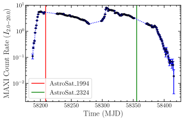
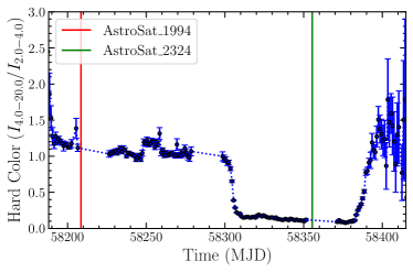
Figure 1: MAXI light-curve in the energy band 2.0 – 20.0 keV (upper panel), and hardness-time diagram (lower panel) of MAXI J1820+070 during 2018 outburst. The hardness is defined as the ratio between the MAXI count-rate in the $4.0-20.0$ keV and $2.0-4.0$ energy bands. Two vertical lines on each panel designate the AstroSat observations.

2.1 AstroSat/SXT

The SXT (Singh et al., 2016, 2017) is equipped with X-ray optics and a CCD camera, and operates in the photon counting mode. It is well suited for medium resolution spectroscopy (FWHM $\sim 150{\rm~{}eV}$ at $6{\rm~{}keV}$) in the $0.5-7{\rm~{}keV}$ band, and is also capable of low resolution imaging (FWHM $\sim 2{\rm~{}arcmin}$, HPD $\sim 11{\rm~{}arcmin}$). We process the level-1 data using the SXT pipeline (AS1SXTLevel2-1.4b) available at the SXT payload operation center (POC) website, and generate level-2 clean event files for individual orbits. For each observation, we merge the orbit-wise clean event files using the Julia SXT event merger tool SXTMerger.jl. We obtain the processed and cleaned level-2 data for a net SXT exposure time of $\sim 17.97{\rm~{}ks}$ and $\sim 7.93{\rm~{}ks}$ for the first and second AstroSat observations.

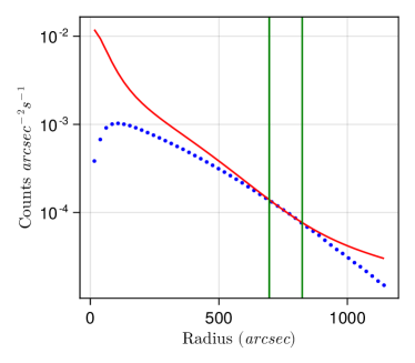
Figure 2: The SXT radial profile of MAXI J1820+070 in the soft state (shown in blue dots) compared with the SXT PSF (represented by a red line). The vertical lines mark the inner and outer radii within which the radial profile matches well with the SXT PSF, and therefore free of significant pile-up. See Section 2.1 for details.

MAXI J1820+070 was very bright, exceeding the Crab flux in the $2-10{\rm~{}keV}$ band in both the hard and soft states, and thus causing severe pile-up in the SXT data. To correct for the pile-up, we first generate SXT radial profile of a blazar Mrk 421 that is bright but not affected with any pile-up. We then model the radial profile with a Moffat function and a Gaussian profile, and derive the PSF of the SXT as,

$$PSF(r)=A\left(\frac{1}{\left\{1+(\frac{r}{r_{c}})^{2}\right\}^{1.04}}+0.08\times\exp{\left\{-\frac{r^{2}}{2\sigma^{2}}\right\}}\right),$$ (1)

with $r_{c}=65.3{\rm~{}arcsec}$, $\sigma=294.2{\rm~{}arcsec}$. We then fit this PSF with a variable amplitude $A$ to the radial profile of MAXI J1820+070 and obtain the range of radii where the radial profile is well described by the SXT PSF, and the corresponding annular region is free of pile-up. We find that the annular regions with inner and outer radii of $r_{i}=800{\rm~{}arcsec}$ (194 pixels) and $r_{o}=900{\rm~{}arcsec}$ (218 pixels) for the soft state, and $r_{i}=618{\rm~{}arcsec}$ (150 pixels) and $r_{o}=907{\rm~{}arcsec}$ (220 pixels) for the hard state are not affected with photon pile-up significantly. In Figure 2, we show the radial profile of MAXI J1820+070 (blue dots) in the soft state and the SXT PSF (red line). The vertical lines mark the annular region between $r_{i}$ and $r_{o}$ that is free from significant pile-up. The deficit of counts in the outermost regions is caused by the loss of events beyond the detector boundary due to the off-axis observations and large PSF/HPD of the SXT.

We use the xselect tool and extract the source spectrum from the merged level-2 event files using an annular region with $r_{i}$ and $r_{o}$ inferred above. Clearly, the ancillary response file (ARF) made available for a circular extraction region centred on the source is inappropriate for a heavily piled-up source like in this case, where a large fraction of counts from the inner region are excluded. Therefore, we derive the corrected ARF as follows. We use the SXT observation of Crab which is a standard X-ray calibrator. We first extract the SXT spectra of Crab using the same annular regions we used for MAXI J1820+070 in the soft and hard states. We fit these Crab spectra with an absorbed power-law model with fixed parameters ($N_{\rm H}=3.1\times 10^{21}{\rm~{}cm^{-2}}$, $\Gamma=2.1$, $f_{X}(2-10{\rm~{}keV})=2.4\times 10^{-8}{\rm~{}ergs~{}cm^{-2}~{}s^{-1}}$; see Weisskopf et al. (2010)) using the ARF/RMF provided by the SXT POC, and derive the data-to-model ratio. Using these ratios, we correct the ARF and derive separate ARFs appropriate for the soft and hard states. As a cross-check, we use the corrected ARFs and fit the Crab spectra and obtain spectral parameters similar to those already known.

2.2 AstroSat/LAXPC

The X-ray instrument LAXPC consists of three proportional counters (LAXPC10, LAXPC20, and LAXPC30) operating in the energy range of 3 – 80 keV with a temporal resolution of 10 $\mu s$ (Antia et al., 2017). Out of these three detectors, LAXPC10 has been showing unpredictable high-voltage variations since March 2018, and LAXPC30 was switched off due to a gas leakage (Antia et al., 2021). Thus, we only use data acquired with the detector LAXPC20 in this work. We extract the LAXPC source and background light curves using the software laxpcsoftv3.4.3 . The response files lx20v1.0.rmf and lx20cshm01v1.0.rmf are used for the hard and soft observations, respectively. We group the LAXPC spectra using the FTOOLS package ftgrouppha to have a signal-to-noise ratio of at least 25 per bin.

2.3 AstroSat/CZTI

Cadmium Zinc Telluride Imager (CZTI) is a hard X-ray instrument onboard AstroSat providing spectroscopic observations in 22 – 200 keV energy range and in-direct imaging by employing coded aperture mask (Bhalerao et al., 2017). CZTI consists of four independant quadrants each having an array of 16 CZT detectors and data are available for each quadrant separately. For the analysis of CZTI data, we use CZTI data analysis pipeline version 3.0 along with the associated CALDB . Following the standard pipeline procedure, clean event list are filtered out from the raw event file. From the clean event files, background subtracted source spectra for each quadrant along with associated response matrices are obtained by using cztbindata task of the data analysis pipeline, which employs the mask-weighting technique. We use the optimal binning scheme of Kaastra & Bleeker (2016) to group the CZTI spectra with minimum 25 counts per bin.

2.4 AstroSat/UVIT

The UVIT (Tandon et al., 2017, 2020) consists of three channels providing sensitivity in three different bands – far ultraviolet ($1200-1800$ Å) (FUV channel), near ultraviolet ($2000-3000$ Å; NUV channel), and the visible ($3200-5500$ Å; VIS channel) bands. The FUV and NUV channels are used for scientific observations, while the VIS channel is mainly used for tracking satellite pointing. Both FUV and NUV channels are equipped with a number of broadband filters for imaging with a point spread function (PSF) in the range of $1-1.5{\rm~{}arcsec}$ and slit-less gratings for low resolution spectroscopy. The FUV channel has two slit-less gratings, FUV-Grating1 and FUV-Grating2 (hereafter FUV-G1 and FUV-G2), that are arranged orthogonal to each other to avoid possible contamination along the dispersion direction, due to the presence of neighboring sources in the dispersed image. These two channels operate in the photon counting mode. More details on the performance and calibration of the UVIT gratings can be found in Dewangan (2021).

We obtain the level1 data on MAXI J1820$+$070 from the AstroSat archive, and process them using the CCDLAB pipeline (Postma & Leahy, 2017). We generate orbit-wise drift-corrected, dispersed images for each observation. We then align the orbit-wise images and merge them into a single image for each observation. We use the UVITTools.jl package for spectral extraction following the procedures described in Dewangan (2021) and Kumar et al. (2023). We first locate the position of the zeroth order image of the source in the grating images, and then use the centroids, along the spatial direction at each pixel, along the dispersion direction for the $-2$ order. We use a 50-pixel width along the cross-dispersion direction and extract the one-dimensional count spectra for the FUV gratings in the $-2$ order. Following a similar procedure, we also extract background count spectra from source-free regions, and correct the source spectra for the background contribution. We use an updated version of grating responses which are adjusted to match a simultaneous hard state HST spectrum of this source (a detailed analysis of the HST spectrum will be discussed on the forthcoming paper, Georganti et. al. 2023). These files are thus generated following the procedures described in Dewangan (2021).

2.5 NICER

In this work, we consider two NICER observations, which were quasi-simultaneous with the AstroSat hard state observation (see Table 1). The NICER data are reduced and calibrated using the NICERDAS 2022-01-17_V009 and CALDB version xti20210707. The NICER X-ray Timing Instrument (Gendreau et al., 2016) consists of an array of 56 co-aligned X-ray concentrator optics, each of which is paired with a single-pixel silicon drift detector working in the 0.2 –- 12 keV energy band (with a spectral resolution of $\sim 85$ eV FWHM at 1 keV and $\sim 137$ eV at 6 keV). Although 52 detectors were working at the time of the observation, we exclude data from the detectors numbered 14 and 34 as they sometimes exhibit periods of increased noise. We generate cleaned event files of the NICER observations using the script nicerl2 (with default criteria) and employ the background estimator nibackgen3C50 (Remillard et al., 2021) to generate the source and background spectra. The scripts nicerarf and nicerrmf are used to obtain the ARF and RMF files for all the NICER observations. We further obtain background uncorrected NICER light-curves in three energy bands: 2.0 – 4.0 keV, 4.0 – 10.0 keV, and 0.6 – 10.0 keV (with 64s bin time) to produce the NICER hardness-intensity (see Fig. 3) diagram. In our work, the NICER hardness is the ratio between the NICER count-rate in the 4.0 – 10.0 keV and 2.0 – 4.0 keV bands. We do not find any significant hardness variation between the two NICER observations (see Fig. 3), and also within a single observation. Hence, we consider these two observations entirely in the present work. We group the NICER spectra using the FTOOLS package ftgrouppha to a signal-to-noise ratio of at least 50 per bin.

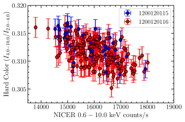
Figure 3: NICER hardness-intensity diagram for the two observations: 1200120115 and 1200120116. The hardness is defined as the ratio between the NICER count-rate in the $2.0-4.0$ keV and $4.0-10.0$ energy bands.

2.6 LCO

MAXI J1820+070 was monitored during its 2018 outburst in the optical wavelengths by the Las Cumbres Observatory (LCO), as part of an on-going monitoring campaign of $\sim$50 low mass X-ray binaries coordinated by the Faulkes Telescope Project (Lewis, 2018). For this study, we use the optical observations obtained with the 1-m robotic telescopes at the LCO nodes of Cerro Tololo Inter-American Observatory (Chile) and South African Astronomical Observatory, Sutherland (South Africa), that were simultaneous/quasi-simultaneous with the hard state and the soft state observations of Astrosat, respectively (see Tables 1 and 2). The observations were performed in the SDSS $g^{{}^{\prime}}$, $i^{{}^{\prime}}$ and $r^{{}^{\prime}}$ bands, with 20 second exposure times on each filter for hard state, and 40 second exposure times for the soft state. We use the “X-ray Binary New Early Warning System (XB-NEWS)” data analysis pipeline (Russell et al., 2019b; Pirbhoy et al., 2020) for calibrating the data, computing an astrometric solution for each image using Gaia DR2 positions, performing aperture photometry of all the stars in the image, solving for zero-point calibrations between epochs, and flux calibrating the photometry using the ATLAS All-Sky Stellar Reference Catalog (ATLAS-REFCAT2) (Tonry et al., 2018).

Table 1: Details of AstroSat and NICER observations used in this study.

Mission	Obs ID	Instrument	Exposure (ks)	Start Time (UT)	End Time (UT)	State
				yyyy-mm-dd/hh-mm-ss	yyyy-mm-dd/hh-mm-ss
AstroSat	T02$\_$038T01$\_$900001994	SXT	17.97	2018-03-30/10:45:52	2018-03-31/14:13:04	Hard
	(AstroSat$\_1994$)	LAXPC	37.78	2018-03-30/10:45:51	2018-03-31/14:13:05
		CZTI-Quad0	37.17	2018-03-30/10:46:36	2018-03-31/14:13:04
		CZTI-Quad1	37.04	,,	,,
		CZTI-Quad2	37.18	,,	,,
		CZTI-Quad3	34.69	,,	,,
		UVIT/FUV-G1	11.39	2018-03-30/12:02:29	2018-03-31/14:11:17
NICER	1200120115 (NICER-1)	XTI	3.34	2018-03-30/09:15:40	2018-03-30/11:30:20	Hard
	1200120116 (NICER-2)	XTI	10.71	2018-03-31/08:28:18	2018-03-31/19:33:09	,,
AstroSat	T02$\_$066T01$\_$900002324	SXT	7.929	2018-08-25/11:10:10	2018-08-25/16:37:28	Soft
	(AstroSat$\_2324$)	LAXPC	11.5	,,	2018-08-25/16:37:29
		UVIT/FUV-G1	2.845	2018-08-25/11:18:01	2018-08-25/13:20:09
		UVIT/FUV-G2	2.739	2018-08-25/14:32:54	2018-08-25/16:35:03

Table 2: Details of LCO observations used in this study.

Filter	Wavelength	Wavelength	Exposure (s)	Date	Time (UT)	State
	center (nm)	width (nm)		yyyy-mm-dd	hh-mm-ss
SDSS-i’	754.5	129	20	2018-03-31	7:32:59	Hard
SDSS-r’	621.5	139	20		7:37:17
SDSS-g’	477.0	150	20		7:34:17
SDSS-i’	754.5	129	40	2018-08-24	21:16:53	Soft
SDSS-r’	621.5	139	40		21:22:44
SDSS-g’	477.0	150	40		21:18:29

3 Spectral Analysis

All spectral analyses presented in the following sections are performed using XSPEC (Arnaud, 1996) version 12.12.1. A multiplicative cross-normalization constant (implemented using constant in XSPEC) is allowed to vary freely for LAXPC, CZTI, XTI/NICER, and fixed to unity for SXT. We consider an energy range of $6.9-9.5$ eV for FUV-G1/FUV-G2, $0.6-7.0$ keV for SXT, $4.0-60.0$ keV for LAXPC (for the hard state observation), $25.0-150.0$ keV for CZTI, and $0.6-10.0$ keV for XTI/NICER. We limit the LAXPC data to $40$ keV for the soft state observation as the spectrum is background dominated beyond that. A systematic error of $2\%$ for all the AstroSat instruments (and LCO filters) and $1\%$ for NICER (as suggested by the their respective instrument teams) is considered in this work. We apply a gain correction to the SXT data using the XSPEC command gain fit with the slope fixed to unity. The best-fit offset is found to be $\sim 0.24$ eV for both the hard state and soft state observations.

We use tbabs (Wilms et al., 2000) to take account for the absorption of X-rays in the interstellar medium along the line of sight. We adopt abundances from Wilms et al. (2000) (wilm in XSPEC), and the photoelectric absorption cross-sections from Verner et al. (1996) (vern in XSPEC). Furthermore, we assume a distance to the source of 2.96 kpc (Atri et al., 2020). The uncertainties reported in this work corresponds to $90\%$ confidence level for a single parameter of interest.

3.1 Hard State

3.1.1 X-ray spectral Analysis

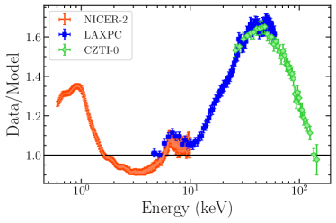
Figure 4: Ratio (Data/Model) of the $0.6-150.0$ keV NICER and AstroSat data to the fiducial model tbabs*constant*cutoffpl (hard state observation). This exercise is performed just to show different spectral features in the hard state spectra. We clearly see a soft excess, the Fe K-$\alpha$ emission line, and a Compton hump with a peak around $\sim 40$ keV in the hard state spectra. Only data from the second NICER observation, LAXPC data, and CZTI Quadrant-0 data are used for this investigation. Data are rebinned for plotting purpose. See Section 3.1.1 for more details.

We begin our investigation with the hard state X-ray data in the energy range of $0.6-150.0$ keV with an absorbed cutoff power-law (i.e., tbabs*constant*cutoffpl in XSPEC notation). We perform this analysis just to demonstrate different spectral features in the data and consider only the data from the second NICER observation, the LAXPC data, and CZTI Quadrant-0 data for this purpose. We note a soft-excess, a broad iron emission line around 6.4 keV, and a Compton hump with a peak at approximately 40 keV in the hard state spectra (see Fig. 4).

We first fit the broadband continuum of the hard-state X-ray data (in the energy range $0.6-150.0$ keV) of MAXI J1820+070 with a simple model (Model: tbabs*constant*(diskbb+nthcomp)) composed of a diskbb (Mitsuda et al., 1984; Makishima et al., 1986) component (for describing the multicolored black-body emission from a geometrically thin and optically thick accretion disk), and a thermal Comptonized component nthcomp (Zdziarski et al., 1996; Życki et al., 1999) (accounting for the hard coronal emission) in which the soft seed photons are provided by the accretion disk (i.e., inp_type of nthcomp has been set to 1). The seed photon temperature of nthcomp is tied to the inner disk temperature of diskbb. This model poorly describes the data ($\chi^{2}/\text{d.o.f}=7627.7/2398$, where $\text{d.o.f}$ stands for degrees of freedom). To obtain a better fit and explore the possibility of another coronal component, we add a second nthcomp to the above model (Model : tbabs*constant*(diskbb+nthcomp(1)+nthcomp(2))). We tie the seed photon temperature of the two Comptonization components to that of the diskbb component. The fit quality improved significantly, giving a $\chi^{2}/\text{d.o.f}=7081.3/2395$ (F-test probability of chance improvement $\sim 10^{-38}$). This improvement is not surprising, as earlier studies have shown (Buisson et al., 2019; Chakraborty et al., 2020; Zdziarski et al., 2021a, 2022b) that the double coronae model offers a better fit to the data. In both these models, the neutral hydrogen column density ($N_{\rm H}$) lies in the range of $1.2-1.4\times 10^{21}\ \rm atoms\ cm^{-2}$, which is close to the Galactic absorption column along the direction of the source, $1.3\times 10^{21}\ \rm atoms\ cm^{-2}$ (HI4PI Collaboration et al., 2016). So, hereafter, we will fix $N_{\rm H}$ to the Galactic value for all subsequent spectral analyses performed on the hard state observation. The residuals for both these models are depicted in Fig. 5. Although the diskbb component has already taken care of the soft excess (seen in Fig. 4), we still observe significant residuals around 1 keV in both of these models, which could be indicative of a reflection feature (see Fig. 5).

However, still, we could not obtain a reasonably good fit, probably due to the strong presence of reflection features (see Fig. 4). Thus, we add a Gaussian component to our double Comptonization model to represent the Fe-K$\alpha$ line observed in the spectra and obtain a huge improvement in the spectral fit (Model: tbabs*constant*(diskbb+nthcomp(1)+nthcomp(2)+ gauss)) with $\chi^{2}/\text{d.o.f}$ of 3921.7/2392. The residuals around 6.5 keV reduces significantly in this model (see Fig. 5). But the low and high-energy residuals do not improve much. The cross-normalization constant between SXT and LAXPC or CZTI (Quadrant-0/1/2/3) or NICER-1/NICER-2 is found to lie in the range of $\sim 0.74-0.91$ ($\sim 9\%-26\%$), which is within the acceptable limit. The peak energy and width of the iron K$\alpha$ line come out to be $6.58\pm 0.02$ keV and $0.77\pm 0.02$ keV, respectively. The equivalent width corresponding to this line for the NICER data is found to be $0.18\pm 0.33$ keV. The inner disk temperature is $0.27\pm 0.05$, which is close to the value of $\sim 0.2$ keV obtained earlier for the hard state NICER observations (Dziełak et al., 2021; Wang et al., 2020). The two Comptonization components are well separated in power-law indices ($\Gamma$) and electron temperatures ($kT_{\rm e}$) in this model, with the best-fit values of them being $\Gamma=1.72\pm 0.01$ and $kT_{\rm e}=243.1_{-65.6}^{+46.9}$ and $\Gamma=1.18\pm 0.04$ and $kT_{\rm e}=13.40\pm 0.69$ keV, respectively. Although adding a Gaussian line to our single Comptonization model provides a huge improvement like the previous case, it still could not produce an acceptable fit ($\chi^{2}/\text{d.o.f}=5507.3/2395$). Since other reflection features like the Compton hump are quite prominent in this observation (see Fig. 4), we perform an in-depth reflection analysis of joint AstroSat and NICER data.

For a detailed investigation of the broadband spectra and the reflection features, we use a self-consistent reflection model reflionxhd, the latest model from the reflection suite reflionx (Ross & Fabian, 2005, 2007). The reflionx based reflection models generate an angle-averaged reflection spectrum for an optically-thick atmosphere (such as the surface of an accretion disk) with constant density irradiated by hard Comptonized emission. This new model reflionxhd assumes that the illuminating continuum (responsible for ionizing the disk) is based on the nthcomp Comptonization model (as opposed to a cutoff power-law), with the soft seed photons being provided by the accretion disk (Jiang et al., 2020; Connors et al., 2021; Chakraborty et al., 2021). Besides, the density of the disk ($n_{\rm e}$) is a model parameter in the range of $15\leq\log{(n_{e}/{\rm cm^{-3}})}\leq 22$. We further convolve this component with relconv (Dauser et al., 2010), which is part of the relxill distribution of models (Dauser et al., 2014; García et al., 2014), to consider the effect of relativistic blurring. We add them to our double Comptonization model to represent the relativistically smeared reflected emission. We tie the power-law index ($\Gamma$), electron temperature ($kT_{\rm e}$), and seed photon temperature $kT_{\rm seed}$ of the reflionxhd component (i.e., parameters related to the input continuum) with one of our external nthcomp components. The ionization parameter ($\xi$), iron-abundance ($A_{\rm Fe}$), and density ($\rm log$$(n_{\rm e})$) are left as free parameters. On the other hand, in relconv, we fix the spin of the BH (i.e., Kerr parameter) to $a=0.998$ (i.e., the ISCO radius or radius of innermost stable circular orbit around a Kerr BH, $R_{\rm ISCO}=1.237\ R_{g}$, where $R_{g}=GM/c^{2}$, $M$ is the mass of the BH, $G$ is the Newtonian gravitational constant, and $c$ is the speed of light in free space) to enable comparisons with previous studies, as this assumption has been made in all the works that performed reflection analysis in the hard state (Buisson et al., 2019; Chakraborty et al., 2020; Zdziarski et al., 2021a, 2022b). Since the outer accretion disk could be misaligned with respect to the BH spin axis (Poutanen et al., 2022; Thomas et al., 2022), we assume that the inclination of the inner disk is identical to that of the jet, i.e., $i=64^{\circ}$ (Wood et al., 2021), which is presumed to be in the direction of the BH spin axis. We also assume a single emissivity index ($q=q_{1}=q_{2}$), making the break radius (which separates the inner disk with emissivity $q_{1}$ from the outer disk with emissivity $q_{2}$) redundant, and set the outer disk to $1000R_{g}$. To account for the narrow core of the Fe-K$\alpha$ line, we add another reflionxhd component to our existing model and tie the parameters of the internal nthcomp part ($\Gamma$, $kT_{\rm e}$, and $kT_{\rm seed}$) of reflionxhd with those of another external nthcomp component in our existing model. Additionally, we tie the density and iron-abundance of this reflection component to the previously added reflionxhd. The density of the disk associated with these two reflection components (relativistic and distant) is perhaps different. However, we tie them to keep our model simple by reducing the number of free parameters. Thus, in the present model (hereafter referred to as Model 1A), one nthcomp (i.e., nthcomp(1)) component gets reflected through the relativistic reflection component relconv*reflionxhd(1), and another one, i.e., nthcomp(2) through the distant reflection component reflionxhd(2). We link the seed photon temperature of these two Comptonization components to the inner disk temperature of the diskbb component. Therefore, the resulting model takes the following form,

• Model 1A: tbabs*constant*(diskbb+nthcomp(1)
  +nthcomp(2)+relconv*reflionxhd(1)
  +reflionxhd(2)).

We obtain a $\chi^{2}/\text{d.o.f}$ of 1904.2/2388, i.e., a huge improvement in the spectral fit compared to our previous models. The results are presented in Table 3 and the residuals are depicted in Fig. 5.

We first notice that the residuals below 2 keV and above 10 keV diminish significantly in this model (see Fig. 5). The disk temperature, in this case, $0.192\pm 0.002$, takes a value almost identical to what was estimated earlier (Wang et al., 2020). Besides, the disk is found to get truncated far from the source, at a distance of $62.3^{+15.2}_{-11.4}\ R_{g}$. We also estimate the inner disk radius from the diskbb normalization following the relation,

$$R_{\rm in}=\eta\kappa^{2}\sqrt{\frac{N_{\rm disk}}{\cos{i}}}\frac{D}{10\ \rm kpc}$$ (2)

where, $R_{\rm in}$ is true inner radius in km, $\kappa$ is the spectral hardening factor (i.e., the ratio between the color temperature to effective temperature) (Shimura & Takahara, 1995), $\eta$ is the correction factor for the inner torque-free boundary condition for a Schwarzschild BH ($a=0$) (Kubota et al., 1998), $N_{\rm disk}$ is the diskbb normalization, and $D$ is the distance to the source. However, it is unlikely that the zero torque condition is applicable in the hard state, where the disk is truncated far from the ISCO radius. Thus, it is perhaps incorrect to include the correction factor $\eta$ in our estimation of true inner radius (see Basak & Zdziarski (2016) for more details). Adopting $\kappa=1.7$ (Kubota et al., 1998), $i=64^{\circ}$, and mass of the BH ($M$)=6.75 $M_{\sun}$ (Mikołajewska et al., 2022), we obtain $R_{\rm in}\sim 73R_{g}$, which is consistent with the value obtained from the reflection fit.

The power-law index and electron temperature of the two Comptonization components are $1.168\pm 0.002$ and $30.55_{-0.99}^{+0.95}$ keV (nthcomp(2)), and $1.596\pm 0.003$ and $15.39\pm 0.34$ keV (nthcomp(1)), respectively. The reflecting part of the disk corresponding to the soft Comptonization component is found to be strongly ionized $\xi=2365_{-47}^{+64}$ compared to that ($\xi=488_{-12}^{+14}$) illuminated by the hard Comptonization component. Similar two-component Comptonization scenarios with other reflection models (e.g., relxilllpCp) were investigated earlier by Buisson et al. (2019); Chakraborty et al. (2020); Zdziarski et al. (2021a, 2022b), and in all these works, it was noted that a double coronae model provides a much better fit to data than a single corona model. The values of the best-fit parameters in Model 1A are consistent with those obtained in an earlier investigation of this source with contemporaneous Insight-HXMT, NuSTAR, and INTEGRAL data (Zdziarski et al., 2022b). Notably, in all the above analyses, constant density reflection models (i.e., $n_{\rm e}$ is fixed at $10^{15}\ \rm cm^{-3}$) were employed. In some of these works (Buisson et al., 2019; Chakraborty et al., 2020), a higher iron abundance ($>3A_{\rm Fe,solar}$) was reported. In our work, $\rm log$$(n_{\rm e})$ is a variable parameter, and it takes a higher value of $20.32\pm 0.04$. Moreover, $A_{\rm Fe}$ is almost close to the solar abundance, which is expected as the secondary star is a weakly evolved low-mass donor star (Mikołajewska et al., 2022). We will discuss the inner disk geometry of the hard state in detail in Section 4.1.

In this model (Model 1A), we additionally perform fitting with leaving the inclination, and emissivity index as free parameters. But, their values remain unconstrained in their allowed ranges. We also consider a single Comptonization model for performing this reflection study, by tying $\Gamma$, $kT_{\rm e}$, and $kT_{\rm seed}$ of two reflionxhd components with that of a single nthcomp component. This model results in a poorer fit, with $\chi^{2}/\text{d.o.f}=2546.3/2391$. Additionally, $kT_{\rm in}$ is found to be quite low $\sim 0.1$ keV and the disk is estimated to have reached almost the ISCO radius, $=2.4\pm 0.3\ R_{\rm ISCO}$, inconsistent with the same calculated from the diskbb normalization. Furthermore, we observe significant residuals above 100 keV, which progressively increase with energy (see Fig. 5). Therefore, Model 1A not only provides a better statistical description of the data but also yields physically consistent values for all model parameters. We will further consider this model for the multi-wavelength spectral analysis of this source in the hard state.

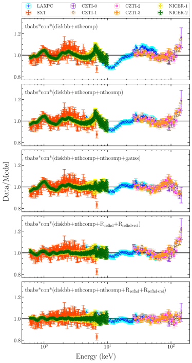
Figure 5: Ratio (Data/Model) of the $0.6-150.0$ keV X-ray multi-instrument (AstroSat+NICER) data to several models for the hard state observation. Here, $R_{\rm refhd}$ and $R_{\rm refhd*rel}$ stand for reflionxhd and relconv*reflionxhd. In this plot, the model components are mentioned on top of each panels. The panels, from top to bottom, illustrate the improvement in residuals as further model components are added. Data are rebinned for plotting purpose. See Section 3.1.1 for more details.

3.1.2 UV Spectral Analysis

We fit the FUV-G1 spectrum in the energy range 6.9 – 9.5 eV with an absorbed black-body model (Model: redden*bbodyrad) (Meshcheryakov et al., 2018) and obtain a $\chi^{2}/\text{d.o.f}$ of $661.6/175$. Here, we fix the color excess $E(B-V)$ to 0.17 corresponding to the neutral hydrogen column density of $1.3\times 10^{21}\ \rm atoms\ cm^{-2}$ along the source line of sight via equation 15 of Zhu et al. (2017), which is also close to the earlier estimated value of $E(B-V)=0.163\pm 0.007$ (Baglio et al., 2018). We clearly observe residuals around $7.55$ eV, $8.0$ eV, and $8.89$ eV (see Fig. 6). The residuals around these three energy values most likely correspond to the emission lines: He II $\lambda$1640.4, C IV $\lambda$1549.1, and Si IV $\lambda$1396.8 (Vanden Berk et al., 2001). We add three Gaussian lines (gauss in XSPEC notation) to account for these features, and notice that the Gaussian width ($\sigma$) of the emission line Si IV is significantly broader than the other lines. The Si IV line is probably a doublet, with components at $1393\rm\AA$ and $1403\rm\AA$ (Morton, 2003), which is responsible for making this line broader. Additionally, this feature is sometimes contaminated by or potentially even dominated by a semi-forbidden emission line O IV] $\lambda$1402.1 (Vanden Berk et al., 2001). We tie the line-widths of He II and C IV lines, and leave that of Si IV as a free parameter. Thus, our new model (hereafter, Model 1B) becomes:

• Model 1B: redden*(gauss(He II)+gauss(C IV)
  +gauss(Si IV)+bbodyrad(UV)).

This model provides a $\chi^{2}/\text{d.o.f}$ of $222.1/165$. The results are presented in Table 4, and the unfolded spectrum and residuals in the form of a ratio (model/data) are depicted in Fig. 7.

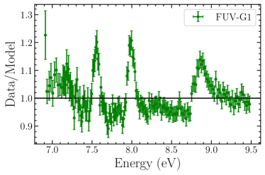
Figure 6: Ratio of the 6.9 – 9.5 eV FUV-G1 data to the model redden*bbodyrad (hard state observation). The residuals around $7.55$ eV, $8.0$ eV, and $8.89$ eV are clearly observed. See Section 3.1.2 for more details.

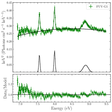
Figure 7: Unfolded spectrum with model (Model 1B) components in black (upper panel) and ratio of the 6.9 – 9.5 eV FUV-G1 data to Model 1B (lower panel) (hard state observation). See Section 3.1.2 for more details.

3.1.3 Broadband Optical/UV/X-ray Spectral Analysis

We will now perform a multi-wavelength spectral study of this source in the energy range 1.64 eV – 150 keV and investigate the correlation between the spectral parameters in the X-ray and optical/UV bands. We first add the FUV-G1 spectral data to our X-ray datasets and extrapolate the best-fit X-ray model (Model 1A). We observe a huge UV excess below 0.01 keV (see Fig. 8). This indicates that our X-ray model severely underestimates the UV flux, implying the dominance of the effect of irradiation in the outer accretion disk (Gierliński et al., 2009). Thus, we add our best fit UV model, Model 1B, to the X-ray spectral model 1A to describe the UV emission in the hard state spectra. We set $N_{\rm H}=0$ for the FUV-G1 spectrum and $E(B-V)=0$ for the X-ray part of the spectra. Additionally, we fix the Gaussian centroid energies and widths of the emission lines, and the bbodyrad temperature in this model to their respective values in Model 1B, and keep only the normalization of these components as free parameters. The parameter constant is also kept frozen to unity for the FUV spectrum. Thus, the present model takes the form, tbabs*redden*constant*(diskbb+nthcomp(1) +nthcomp(2)+reflionxhd+relconv*reflionxhd+ gauss(He II)+gauss(C IV)+gauss(Si IV)+bbodyrad(UV). We obtain a $\chi^{2}/\text{d.o.f}$ of 2152.5/2561. Finally, we add LCO data to this setup and find an unacceptable fit with a $\chi^{2}/\text{d.o.f}$ of 6543.5/2564. We note that adding LCO data to our previous model results in significant residuals below 5 eV (see Fig. 9). To circumvent the issue, we add another bbodyrad component to this model to take care of the excess observed in the mentioned energy band. This results in our model, Model 1C:

• Model 1C: tbabs*redden*constant*(diskbb
  +nthcomp(1)+nthcomp(2)+reflionxhd(2)
  +relconv*reflionxhd(1)+gauss(He II)
  +gauss(C IV)+gauss(Si IV)+bbodyrad(UV)
  +bbodyrad(optical)).

We observe a substantial improvement in the spectral fit, $\chi^{2}/\text{d.o.f}=2157.7/2562$, and the previously mentioned residuals consequently decrease significantly (see Fig. 10). Besides, all the X-ray spectral parameters in this new model take almost identical values to the same parameters of Model 1A, i.e., the previous spectral fit does not get affected due to the inclusion of LCO data. The results are given in Table 5 and the broadband unabsorbed SED (along with residuals) is provided in Fig. 10. We estimate the reprocessed fraction in this model by taking the ratio of the flux in the 0.5 – 10.0 eV band (the flux contribution below 0.5 eV is $\lesssim 1\%$) to that in the 0.1 – 200.0 keV band, and find this quantity to be $\sim 9\times 10^{-3}$. Since the outer disk can emit a significant fraction of photons in the 0.5 – 10.0 eV band through viscous dissipation, we consider only the flux of two bbodyrad components and 3 emission lines in that band for calculating the value of reprocessed fraction.

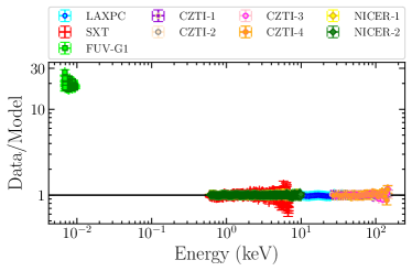
Figure 8: Ratio (Data/Model) of the 0.0069 – 150.0 keV multi-wavelength (AstroSat+NICER) data to the model: Model 1A (hard state observation). We see a huge UV excess below 10 eV. See Section 3.1.3 for more details.

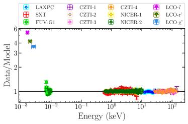
Figure 9: Ratio (Data/Model) of the 0.00164 – 150.0 keV multi-wavelength (AstroSat+NICER+LCO) data to the combined model: Model 1A + Model 1B (hard state observation). We note an optical excess below 5 eV. See Section 3.1.3 for more details.

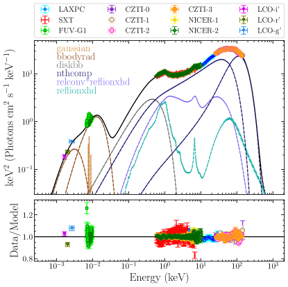
Figure 10: Broad-band (Optical to hard X-ray) unabsorbed SED (upper panel) and residuals (lower panel), in the form of ratio (data/model), corresponding to Model 1C (hard state observation). The total model is represented by a solid black line in the upper panel. Data are rebinned for plotting purpose. See Section 3.1.3 for more details.

3.2 Soft State

3.2.1 X-ray Spectral Analysis

We fit the SXT+LAXPC soft state spectra in the $0.6-40.0$ keV band with a model comprising a multicolored disk black-body component (diskbb; Mitsuda et al. 1984; Makishima et al. 1986) and a thermal Comptonization component (thcomp; Zdziarski et al. 2020) to describe the weak Comptonization in the soft state. We additionally require a single-temperature black-body component (bbodyrad) to achieve a good fit (F-test probability of chance improvement is $\sim 10^{-90}$). The black-body component was earlier detected with the NuSTAR data with similar parameters, and proposed to represent the radiation from the plunging region (Fabian et al., 2020). The Comptonization component thcomp is described by 3 parameters: $\Gamma$, $kT_{\rm e}$, and covering fraction $cov\_frac$. We convolve this component over diskbb and bbodyrad, as both of them can provide soft seed photons for Comptonization. Thus, we finally arrive at a simple three component model,

• Model 2A: tbabs*constant*thcomp*(diskbb
  +bbodyrad).

A similar model was earlier used by Fabian et al. (2020) to describe the broad-band soft-state NuSTAR spectra of this source. In their model, a cutoffpl component was employed to describe the weak Comptonization component, rather than a more physically meaningful thcomp component. Our Model 2A reasonably describes the soft-state spectrum, yielding a $\chi^{2}$/d.o.f of 490.1/413. The best-fit parameters for this model are listed in Table 6. The value of the cross-normalization factor between SXT and LAXPC is found to be $1.21\pm 0.05$ ($\sim 20\%$), which falls within the accepted limit (Antia et al., 2021). We obtain a hydrogen column density ($N_{H}$) of $\sim 0.8\times 10^{21}\ \rm atoms\ cm^{-2}$, which is close to the Galactic column density in the direction to the source, $1.3\times 10^{21}\ \rm atoms\ cm^{-2}$ (HI4PI Collaboration et al., 2016). The disk ($kT_{\rm in}$) and black-body ($kT_{\rm BB}$) temperatures, and the electron temperature, $kT_{\rm e}$ ($0.58\pm 0.02$ keV, $0.79\pm 0.02$ keV, and $>36.5$ keV, respectively) are found to be roughly consistent with the nearest ($0.64\pm 0.01$, $0.92\pm 0.02$, and $64.6_{-26}^{+116}$, respectively) NuSTAR observation (Fabian et al., 2020) (Observation Nu31 in their paper; the AstroSat observation was performed $\sim 6$ days after the Nu31 observation). Furthermore, we find the value of $cov\_frac\sim 5\times 10^{-3}$ to be quite small, implying a very weak Comptonization component. The bbodyrad normalization implies that the X-ray emission is coming from a radius of $\simeq 42-53$ km, considering $D=2.96$ kpc and $\kappa=1.7$. This region is found to be smaller than the true inner disk radius, $\simeq 88-99$ km, as estimated from the diskbb normalization using equation (2) (we consider $\kappa=1.7$, $\eta=0.4$, $i=64^{\circ}$ and $D=2.96$ kpc for this calculation). Since the disk fraction is $\sim 85\%$ (i.e., the fraction of disk flux to the total flux in the 0.1-200.0 keV range) in this observation, the inner disk can be assumed to reach the ISCO radius (McClintock et al., 2014). Therefore, the X-ray emission associated with the bbodyrad component could be related to the radiation coming from the plunging region (Fabian et al., 2020).

We will now replace the diskbb component with a more sophisticated model kerrbb (Li et al., 2005) to describe the emission from a geometrically thin and optically thick accretion disk around a spinning BH (i.e., a Kerr BH). This model takes into account general relativistic effects such as frame-dragging, Doppler boost, gravitational redshift, and bending of light caused by the gravity of a Kerr BH. The spin and mass of the BH, along with the inclination of the inner accretion disk, serve as input parameters for the kerrbb model, in addition to the distance to the source, which we fix at 2.96 kpc, as determined in Atri et al. (2020). In our spectral analysis, we incorporate the effects of both limb-darkening and returning radiation by setting both r_flag and l_flag of kerrbb to 1. In addition, we set the spectral hardening factor to the default model value of $\kappa=1.7$. Thus, the new model takes the form,

• Model 2B: tbabs*constant*thcomp*(kerrbb
  +bbodyrad)

Fitting this model to the data gives a $\chi^{2}$/d.o.f of 464.1/410. The results from the fit are presented in Table 6. The value of $N_{\rm H}$ ($\sim 1.10\ \times 10^{21}\ \rm atoms\ cm^{-2}$) is found to be close to that of Model 2A, and the cross-normalization constant a little higher, $1.25\pm 0.06$.

The spin ($a$) and mass ($M$) of the BH in this model come out to be $>0.84$ and $9.73_{-2.52}^{+2.25}\ \rm M_{\sun}$, respectively, for an inclination of $46.8_{-10.1}^{+4.7}$. Torres et al. (2020) found that the inclination of the binary ($i_{b}$) lies in the range of $66^{\circ}-81^{\circ}$ based on their intermediate-resolution spectroscopic analysis of the optical counterpart of MAXI J1820+070. They also provided a prediction for the BH’s mass: $M=(5.95\pm 0.22)M_{\sun}/\rm sin^{3}i_{b}$. For inclinations between $66^{\circ}-81^{\circ}$, this relationship yields a mass range of $5.73-8.34\ M_{\sun}$, which is slightly smaller than our estimated value. Interestingly, there is a significant discrepancy in the measurement of the spin of this BH between several studies. Zhao et al. (2021) performed a continuum-spectral analysis of this source in the soft state, similar to our approach, but with a different model (kerrbb2) and using Insight-HXMT data. They found a slowly rotating BH with a spin of $0.14\pm 0.09$ ($1\sigma$), assuming a BH mass of $8.48$ and an inclination of the inner disk of $63^{\circ}$. Their analysis also indicated that the BH most likely has a prograde spin if $5.73M_{\sun}<M<8.34M_{\sun}$ and an inclination in the range of $66^{\circ}-81^{\circ}$. On the other hand, Bhargava et al. (2021) analyzed the power-density spectra obtained from NICER high cadence observations of the source in the hard state, and employed relativistic precession model to estimate the spin of the BH. Their analysis yielded a spin value of $a=0.799_{-0.015}^{+0.016}$, which is close to our value. Additionally, our estimation of the inclination angle is significantly lower than the jet inclination angle of $64^{\circ}\pm 5^{\circ}$, which is possibly identical to the angle of the BH’s spin axis (see Liska et al. 2018 for an alternative scenario).

The values of mass and spin of a BH in the kerrbb model strongly depend on the inclination of the inner disk and the distance to the source (McClintock et al., 2014). Therefore, we also perform spectral fitting with Model 2B, with the inclination angle fixed to the jet inclination angle, which could be used as a proxy for the inner disk inclination angle (assuming that the inner disk’s angular momentum is aligned with the BH’s spin axis; however, for other scenarios, see Banerjee et al. (2019a, b)). We obtain a $\chi^{2}$/d.o.f of 467.2/411. The mass and spin values of this source are found to be greater than $5.9M_{\sun}$ and in the range of $0.60-0.95$ (See Table 6), respectively, which are quite consistent with earlier measurements (we restrict the upper limit of the BH mass to $12M_{\sun}$ in our spectral fit). Fabian et al. (2020) employed a similar model, using cutoffpl instead of thcomp to represent the Comptonization component, in their analysis with NuSTAR observations. They fixed the spin (a) and inclination ($i$) at $0.2$ and $34^{\circ}$, respectively, based on the results reported in Buisson et al. (2019). The best-fit temperatures of the black-body ($kT_{\rm BB}=0.84\pm 0.04$ keV) and the Comptonising corona ($kT_{\rm e}>17$ keV) in our model are roughly in agreement with those derived by Fabian et al. (2020) from the nearest NuSTAR observations.

We will finally consider our third model, where we utilize the irradiated disk model diskir (Gierliński et al., 2009) to describe the broad-band X-ray continuum. In addition to this, we use the bbodyrad component mentioned earlier. Apart from describing the emissions from a disk and corona (diskir assumes diskbb and nthcomp routines for this purpose), diskir (has 9 parameters) considers the optical/UV emission resulting from the irradiation of the outer disk by the X-ray emission from the inner accretion disk and corona. Furthermore, this model not only describes the reprocessing of X-rays in the outer accretion disk, but also takes into account the illumination of the inner disk by the Compton tail. In essence, this model considers both the irradiation of the inner accretion disk and the outer accretion disk. We fit the following 5 parameters of diskir (along with the parameters of bbodyrad and tbabs) to the joint SXT-LAXPC data: 1) the temperature of the accretion disk $kT_{\rm disk}$, the normalization (which is identical to the diskbb normalization), power-law index $\Gamma$, electron temperature $kT_{\rm e}$, and a ratio of luminosity in the Compton tail to the unilluminated disk $L_{\rm c}/L_{\rm d}$. Since we are exclusively considering the X-ray part of the total spectra, we will keep the outer disk radius ($\rm log(r_{\rm out})=log(R_{\rm out}/R_{\rm in})$ (where $R_{\rm out}$ and $R_{\rm in}$ denote the outer disk and inner disk radii, respectively) and reprocessed fraction ($f_{\rm out}$: the fraction of bolometric X-ray luminosity thermalized in the outer disk) fixed at 4.5 and 0 (i.e., irradiation of the outer disk is turned off), respectively, as these parameters are constrained from the optical/UV spectrum. We additionally freeze the parameters $f_{\rm in}$ (the fraction of the Comptonized luminosity thermalized in the inner disk) and $r_{\rm irr}$ (the radius of the Compton illuminated disk as a fraction of the inner disk radius) to their default values of $0.1$ and $1.2$, respectively, since they remain unconstrained when left free. Thus, our full model is,

• Model 2C: tbabs*constant*(diskir+bbodyrad).

We obtain a $\chi^{2}$/d.o.f of 490/413. The resulting best-fitting parameters are given in Table 6. The value of disk and black-body temperatures, electron temperature, the power-law index in this model is almost identical to that of Model 2A.

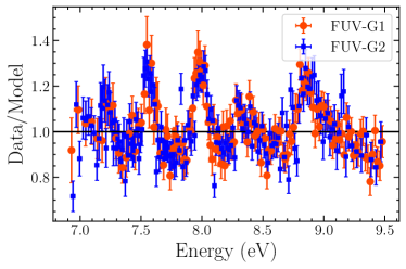
Figure 11: Ratio of the 6.9 – 9.5 eV FUV-G1 and FUV-G2 data to the model redden*bbodyrad (soft state observation). The residuals around $7.21$ eV, $7.55$ eV, $8.0$ eV, $8.34$ eV and $8.89$ eV are clearly observed. See Section 3.2.2 for more details.

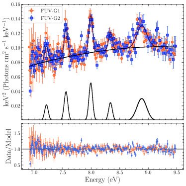
Figure 12: Unfolded spectrum with model (Model 2D) components in black (upper panel) and ratio of the 6.9 – 9.5 eV FUV-G1 and FUV-G2 data to Model 2D (lower panel) (soft state observation). See Section 3.2.2 for more details.

3.2.2 UV Spectral Analysis

From the X-ray spectral fit of the joint SXT+LAXPC data, we find that the hydrogen column density along the source line of sight can be approximated as $\sim 9.0\times 10^{20}\ \rm atoms\ cm^{-2}$, which is roughly the median value in our estimated range. Hereafter, we will fix $N_{\rm H}$ to the above-mentioned value for all subsequent fits in the soft state case. This value corresponds to a color excess of $E(B-V)=0.12$ via equation 15 of Zhu et al. (2017)), which is roughly consistent with the earlier estimated value of $E(B-V)=0.163\pm 0.007$ (Baglio et al., 2018).

We fit the FUV-G1 + FUV-G2 spectra with an absorbed single temperature black-body (Model: redden*bbodyrad) (Meshcheryakov et al., 2018) and obtain a $\chi^{2}$/d.o.f of 895/345. We observe large residuals around $7.21$ eV, $7.55$ eV, $8.0$ eV, $8.34$ eV and $8.89$ eV (see Fig. 11). The residuals around these five energy values most likely correspond to the five emission lines: N IV $\lambda$1718.5, He II $\lambda$1640.4, C IV $\lambda$1549.1, N IV] $\lambda$1486.5, and Si IV $\lambda$1396.8 (Vanden Berk et al., 2001; Harris et al., 2016). We thus add five Gaussian lines to account for these features, and find that the width of the emission line Si IV is significantly broader than the other lines as also noted earlier for the hard state case (see Section 3.1.2 for a discussion on this). Therefore, we tie the width of the Gaussians corresponding to the lines N IV, He II, C IV, and N IV], but leave that of Si IV as a free parameter. Thus, we arrive at our following model:

• Model 2D: redden*(gauss(N IV)+gauss(He II)
  +gauss(C IV)+gauss(N IV])+gauss(Si IV)
  +bbodyrad(UV)).

This model provides a $\chi^{2}$/d.o.f of 408/333. The results are presented in Table 7, and the unfolded spectrum and residuals in the form of a ratio (model/data) are depicted in Fig. 12. The temperature of the black-body component ($kT_{\rm uv}=3.87\pm 0.24$ eV) is found to be slightly higher than the hard state case ($=3.27\pm 0.08$ eV), although the normalization is an order of magnitude smaller than that of the hard state case (i.e., UV flux in the hard state is much higher than the soft state case).

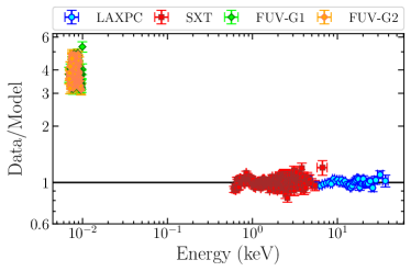
Figure 13: Ratio (Data/Model) of the 0.00690 – 40.0 keV multi-wavelength AstroSat data to the model: Model 2A (soft state observation). We note an UV excess below 10 eV. See Section 3.2.3 for more details.

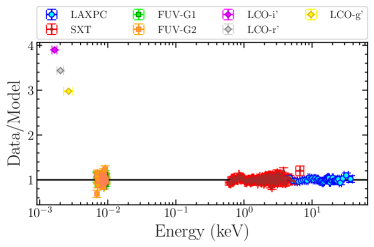
Figure 14: Ratio (Data/Model) of the 0.00164 – 40.0 keV multi-wavelength (AstroSat+LCO) data to the combined model: Model 2A + Model 2D (soft state observation). We see some residuals below 5 eV. See Section 3.2.3 for more details.

3.2.3 Broadband Optical/UV/X-ray Spectral Analysis

We initially add the FUV-G1 and FUV-G2 spectral datasets to our X-ray datasets and extrapolate our best-fit X-ray model (Model 2A) to lower energies, and note a significant UV excess below 10 eV (see Fig. 13). However, the UV excess in the soft state is considerably weaker than what has been observed in the hard state observation. To account for the UV excess, we add our best fit UV model, Model 2D, to the X-ray model. Thus, we perform a joint UVIT+SXT+LAXPC spectral analysis with the combined model: Model 2A + Model 2D. We set the $N_{\rm H}=0$ for the UVIT/FUV spectra and $E(B-V)=0$ for the SXT and LAXPC spectra. Furthermore, we keep all the parameters of Model 2D fixed, except for the normalizations of the individual spectral components. This combined model yields a reasonable fit to the data, with a $\chi^{2}/\text{d.o.f}$ of 888.2/755. Now, LCO data are added to this setup, resulting in a fit with $\chi^{2}/\text{d.o.f}$ of 1781.9/758. We observed some residuals below 5 eV in the present model (see Fig. 14), and add another bbodyrad component empirically to take care of the optical excess, as we did previously for the hard state case. Our new model thus becomes,

• Model 2E: tbabs*redden*constant*(bbodyrad(UV)
  +gauss(N IV)+gauss(He II)+gauss(C IV)
  +gauss(N IV])+gauss(Si IV)+ bbodyrad(optical)
  +thcomp*(diskbb+bbodyrad)).

We achieve a significant improvement in the spectral fit, obtaining a $\chi^{2}/\text{d.o.f}$ of 900.5/756. Consequently, the residuals below 5 eV are also notably reduced (see Fig. 15). The results are given in Table 8. The broad-band unabsorbed SED and the residuals are depicted in Fig. 15. The temperature ($kT_{\rm optical}$) of the new bbodyrad component ($=0.75\pm 0.04$ eV) is found to be close to the same in the hard state case ($=0.80\pm 0.03$ eV). However, the corresponding normalization is substantially smaller, suggesting a higher optical flux in the hard state case. We estimate the reprocessed fraction in this model by taking a ratio of the flux in the 0.5-10.0 eV band (the flux contribution below 0.5 eV is $\lesssim 1\%$) to the flux in the 0.1-200.0 keV band, and find this quantity to be quite smaller ($\sim 3.5\times 10^{-3}$) than the hard state case. While calculating the flux in the 0.5-10.0 eV band for determining the reprocessed fraction, we do not consider the contribution of the disk (i.e., the diskbb flux) since the disk can intrinsically emit a significant fraction of optical/UV photons through viscous dissipation.

Similarly, we add LCO data to the UV/X-ray data, and fit the data with our combined model: Model 2B + Model 2D, and find significant residuals below 5 eV. Therefore, just like the previous case, we consider another bbodyrad component to describe the optical excess, and obtain our new model,

• Model 2F: tbabs*redden*constant*(bbodyrad(UV)
  +gauss(N IV)+gauss(He II)+gauss(C IV)
  +gauss(N IV])+gauss(Si IV)+bbodyrad(optical)
  +thcomp*(kerrbb+bbodyrad)).

We obtain a $\chi^{2}/\text{d.o.f}$ of 881.9/756. Similar to the previous case, the residuals below 5 eV reduces significantly (see Fig. 16). The results are presented in Table 8. The broad-band unabsorbed SED and the residuals are depicted in Fig. 16. In this model, we set the inclination and the mass of the BH to $64^{\circ}$ and $6.75M_{\odot}$, respectively. Additionally, we fix the value of the Kerr parameter at $a=0.75$, which approximately represents the median value within our estimated range for this parameter. Notably, we observe that the spectral parameters in Models 2E and 2F generally exhibit good agreement with each other.

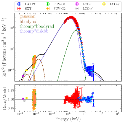
Figure 15: Broad-band (Optical to hard X-ray) unabsorbed SED (upper panel) and residuals (lower panel), in the form of ratio (data/model), corresponding to Model 2E (soft state observation). The total model is represented by a solid black line in the upper panel. Data are rebinned for plotting purpose. See Section 3.2.3 for more details.

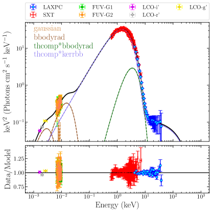
Figure 16: Broad-band (Optical to hard X-ray) unabsorbed SED (upper panel) and residuals (lower panel), in the form of ratio (data/model), corresponding to Model 2F (soft state observation). The total model is represented by a solid black line in the upper panel. Data are rebinned for plotting purpose. See Section 3.2.3 for more details.

Now, we explore whether the necessity of two black-body components is a direct consequence of our choice of $E(B-V)$. To investigate this, we leave both the parameters $N_{\rm H}$ and $E(B-V)$ as free parameters in our Model 2E. This results in a slightly worse fit with a $\chi^{2}/\text{d.o.f}$ of 893.7/754 and a somewhat lower value of $E(B-V)\approx 0.09$ (the value of $N_{\rm H}$ remains close to its fixed value). However, it’s worth noting that the two bbodyrad components and the emission lines remain statistically significant. Subsequently, we fix the values of $N_{\rm H}$ and $E(B-V)$ to $0.13\times 10^{21}\ \rm atoms\ cm^{-2}$ (HI4PI Collaboration et al., 2016) and 0.17, respectively, in our Model 2E, which are the standard values of these quantities in the literature (we consider these values in the hard state case). This results in a significantly poorer fit, with a $\chi^{2}/\text{d.o.f}$ of 1012.8/756. Nevertheless, both bbodyrad components (and the emission lines) remain statistically required to achieve a reasonable fit. In both the cases, our statements regarding the soft state inner and outer geometry do not change.

Finally, we perform a fit to the LCO+UVIT+SXT+ LAXPC data spanning the energy range from 1.64 eV to 40 keV using the combined model: Model 2C + Model 2D. Similar to the previous case, we leave only the normalizations of Model 2D unfrozen, set $E(B-V)=0$ for the X-ray part, and $N_{\rm H}=0$ for the optical/UV part of the spectra. Since we are considering optical/UV data here, we keep the parameters $f_{\rm out}$ and $\rm log$$(r_{\rm out})$ free during the fitting. In this new model, we exclude the bbodyrad component from Model 2D, as the optical/UV continuum is already accounted for by the diskir component through the parameters $f_{\rm out}$ and $log(r_{\rm out})$. Additionally, we find that the emission line N IV becomes statistically insignificant in this model, possibly due to a shift in the UV continuum. So, we remove the Gaussian component corresponding to this line. Therefore, our final model becomes,

• Model 2G: tbabs*redden*constant*(diskir
  +gauss(N IV)+gauss(He II)+gauss(C IV)
  +gauss(N IV])+gauss(Si IV)+bbodyrad).

This model provides a $\chi^{2}/\text{d.o.f}$ of 1230.6/758. The results are given in Table 8, and the unabsorbed SED and residuals are shown in Fig. 17. Thus, this model provides a poorer fit to the data compared to the previous phenomenological models, Model 2E and Model 2F.

The value of the reprocessed fraction ($\sim 2\times 10^{-3}$) obtained from our spectral fit is consistent with that of other BH-LMXBs in the soft state (Gierliński et al., 2009). Since the diskir normalization is identical to the diskbb normalization and $r_{\rm out}=R_{\rm out}/R_{\rm in}$, we can estimate the outer disk radius ($R_{\rm out}$) from the value of $\rm log$$(r_{\rm out})$ ($=4.38\pm 0.02$) using equation (2) (as $R_{\rm in}$ can be estimated from diskir normalization). Adopting $\kappa=1.7$, $\eta=0.4$, and $i=64^{\circ}$, we find that the size of the disk, $R_{\rm out}$, is $(=2.30\pm 0.33\times 10^{11})$ cm. The size of an accretion disk cannot be smaller than the circularization radius due to the conservation of angular momentum, and larger than the tidal truncation radius. To check the consistency of our result, we determine the values of circularization radius ($R_{\rm circ}$) and tidal truncation radius ($R_{\rm tidal}$) using equations (11) and (12) of Gilfanov & Arefiev (2005), respectively. We find that $R_{\rm circ}\simeq 0.27R_{\rm orb}$ ($R_{\rm orb}$ is the orbital separation) and $R_{\rm tidal}\simeq 0.57R_{\rm orb}$, assuming a mass ratio of $q=0.072$ (Torres et al., 2020). We thus use Kepler’s third law of motion to calculate $R_{\rm orb}$, and obtain $R_{\rm orb}\simeq 4.75\times 10^{11}$ cm, considering an orbital period of 16.45 hr for this binary system (Torres et al., 2020). Therefore, $R_{\rm out}$ lies in between $R_{\rm tidal}(\simeq 2.71\times 10^{11}\rm\ cm)$ and $R_{\rm circ}(\simeq 1.28\times 10^{11}\rm\ cm)$. Torres et al. (2020) approximated the outer disk radius at the time of their observation as $0.6b_{1}/R_{\rm orb}$, where $b_{1}$ is the distance of the primary from the $L_{1}$ point. Using equation (4.9) of Frank et al. (2002), one finds out $b_{1}/R_{\rm orb}\simeq 0.76\Rightarrow$ $R_{\rm out}\simeq 2.16\times 10^{11}$ cm. Hence, our estimated value of the disk size is also consistent with earlier reported value.

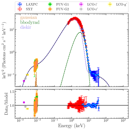
Figure 17: Broad-band (Optical to hard X-ray) unabsorbed SED (upper panel) and residuals (lower panel), in the form of ratio (data/model), corresponding to the Model 2G (soft state observation). The total model is represented by a solid black line in the upper panel. Data are rebinned for plotting purpose. See Section 3.2.3 for more details.

4 Summary of Main Results and Discussion

During the first AstroSat observation in March 2018, MAXI J1820+070 was in the hard state, emitting at an X-ray luminosity (0.1-200.0 keV; hereafter, the total/broadband X-ray flux corresponds to the 0.1-200.0 keV energy range) of $\sim 2\times 10^{38}\ \rm erg\ s^{-1}$ ($\sim 23.5\%$ of Eddington luminosity, calculated assuming $M=6.75M_{\sun}$). Our main results from the multi-wavelength spectral analysis of the hard state data can be summarized as follows.

1. The hard state 0.6 – 150.0 keV X-ray spectra are found to be composed of two Comptonized emission components with different power-law indices and electron temperatures, their associated reflection components, and a disk component with a temperature of $0.19\pm 0.01$ keV (see Section 3.1.1, Figure 10, and Table 3 for more details).

2. The softer Comptonization component ($\Gamma=1.59\pm 0.01$, $kT_{\rm e}=15.39\pm 0.35$ keV) dominates the broadband X-ray luminosity, providing $\sim 50\%$ of the total flux, and gets reflected from a strongly ionized disk ($\xi=2365.5_{-46.9}^{+64.5}{\rm~{}erg~{}cm~{}s^{-1}}$), generating relativistic reflection component. On the other hand, the harder Comptonization component ($\Gamma=1.17\pm 0.01$, and $kT_{\rm e}=30.6\pm 1.0$ keV) contributes $\sim 30\%$ of the total flux and produces unblurred reflection features from a weakly ionized disk ($\xi=488.1_{-12.0}^{+13.8}{\rm~{}erg~{}cm~{}s^{-1}}$), situated far from the ISCO radius.

3. The inner accretion disk is truncated at far from the BH, $\simeq(51-78)R_{g}$ and the density of the disk is quite high, $\sim 2\times 10^{20}{\rm~{}cm^{-3}}$.

4. We detect optical/UV emission in excess of the standard multi-temperature black-body disk emission (see Sections 3.1.2 and 3.1.3, Figures 8 and 9, and Tables 4 and 5 for more details).

5. The UV excess emission is described by a low-temperature black-body of $kT=3.27\pm 0.08$ eV ($37,932\pm 928$ K), and three emission lines: Si IV, C IV and He II (see Figures 6 and 7). Another black-body component with $kT=0.80\pm 0.03$ eV ($9,200\pm 348$ K) accounts for the observed optical excess (see Figure 10).

6. We estimate the reprocessed fraction in the hard state by taking a ratio between the $0.1-200{\rm~{}eV}$ X-ray flux and the $0.5-10{\rm~{}eV}$ optical/UV flux , and find that $0.9\%$ of the bolometric X-ray flux gets reprocessed and thermalized in the outer disk.

During the second AstroSat observation in the soft state, the source was found to accrete at an X-ray luminosity of $\sim 1.1\times 10^{38}\ \rm erg\ s^{-1}$ ($\sim 13\%$ of Eddington luminosity, estimated assuming $M=6.75M_{\sun}$). The main results of our multi-wavelength spectral study of the soft state can be summarized as follows.

1. The soft state X-ray spectrum, in the energy band 0.6 – 40.0 keV, is comprised of a multi-temperature disk component with $kT_{\rm in}=0.58\pm 0.02{\rm~{}keV}$, a soft excess, and a weak Comptonization component ($\Gamma=2.19\pm 0.05$, and $kT_{\rm e}\gtrsim 36.5$ keV; see Section 3.2.1 and Table 6). The soft X-ray excess, which most likely arises from the plunging region (Fabian et al., 2020), is well described by a black-body component with $kT=0.79\pm 0.02{\rm~{}keV}$.

2. Using the continuum fitting method and employing the kerrbb model, we measure the BH spin and mass for the source to be $a=0.85_{-0.25}^{+0.10}$ and $M_{\rm BH}>5.9M_{\sun}$ for an inclination of $64^{\circ}$, which is the jet inclination angle.

3. Similar to the hard state case, we detect optical/UV excess components in the soft state (see Figures 13 and 14), which is comprised of two low-temperature black-body components ($kT=3.87\pm 0.24$ eV and $0.75\pm 0.04$ eV or $kT=44,892\pm 2784$ K and $8704\pm 464$ K) and 5 emission lines: Si IV, N IV], C IV, He II, and N IV (see Sections 3.2.2 and 3.2.3, Figures 11, 12, 15, 16, and 17, and Tables 7 and 8 for more details).

4. The flux in the optical/UV band ($0.5-10$ eV) is found to be significantly smaller than that of the hard state case. Consequently, the reprocessed fraction is low ($\sim 2\times 10^{-3}$), which is directly estimated by fitting the multi-wavelength data to the irradiated disk model diskir. The reprocessed fraction is estimated to be $\sim 3.5\times 10^{-3}$, from the ratio of flux${}^{\ref{foot}}$ in the $0.5-10$ eV to that in the $0.1-200$ keV band. The reduction of optical/UV flux in the soft state (compared to the hard state) has also been noticed earlier for the BH-LMXB XTE J1817-330 (Gierliński et al., 2009).

5. We estimate the outer disk radius directly from our spectral fitting with the diskir model, and find a radius of $(2.30\pm 0.33)\times 10^{11}$ cm, assuming $i=64^{\circ}$.

We discuss below the implications of our multi-wavelength spectral results in the hard and soft states.

4.1 Inner accretion geometry in the hard state

The geometry of the inner accretion flow in the hard state is the subject of ongoing debate. The current paradigm suggests that the disk truncates far from the ISCO radius in the hard state and is replaced by a hot accretion flow (Done et al., 2007). However, this picture has been contested in many works, and an alternative geometry of disk extending into the ISCO radius (or almost ISCO) has emerged (Reis et al., 2010; Kara et al., 2019). For example, Buisson et al. (2019) and Chakraborty et al. (2020) performed reflection analysis of MAXI J1820+070 in the hard state using data from the NuSTAR mission, and found that the disk has reached almost the ISCO radius ($\sim 2-6\ R_{g}$) with their two-component Comptonization model (we have also employed a similar model in our work). Chakraborty et al. (2020) also considered the AstroSat hard state observation and obtained results similar to those from their NuSTAR analysis. In both these works, the inclination was low $\sim 30^{\circ}$ and the iron abundance high, $4-10$ times the solar abundance. Such a high iron abundance is unlikely as the donor star is a low-mass weakly evolved star (Zdziarski et al., 2021a; Mikołajewska et al., 2022). Besides, the binary inclination of the source or the inclination of the jet was estimated to be $>59^{\circ}$.

On the other hand, Zdziarski et al. (2021a, 2022b) also performed reflection analyses using the NuSTAR hard state data (along with INTEGRAL and Insight-HXMT data in the latter work), some of which were considered in the two previously mentioned works, and found the disk to be truncated far from the ISCO radius with a similar double Comptonization model. A similar conclusion regarding the truncation of the inner accretion disk was reported with NICER, NuSTAR, and SWIFT data using the JED-SAD model in Marino et al. (2021).

Unlike the previous works (Buisson et al., 2019; Chakraborty et al., 2020), both the inclination value ($\gtrsim 50^{\circ}$) and the iron abundance ($\sim 1-2.6\ A_{\rm Fe}$) in the studies by Zdziarski et al. (2021a, 2022b) do not suffer from the earlier inconsistencies. Their proposed hard state geometry consists of two Comptonization components: the harder component having a larger scale-height accretion flow located downstream the truncation radius, and the softer component forming a corona over the inner part of the disk. The harder part is reflected from the remote part of a weakly ionized disk, whereas the softer component gets reflected from a highly ionized underlying disk producing narrow reflection features. However, the disk temperature ($\sim 0.4-0.5$ keV) reported in Zdziarski et al. (2022b) is significantly higher than the inner disk temperature obtained with the NICER data (Wang et al., 2020). Finally, in all the above works, the low energy data ($<2.0$ keV) were not used to perform the analysis, and only constant density reflection models, i.e., density ($n_{\rm e}$) is fixed to $10^{15}\ \rm cm^{-3}$, (like relxilllpCp, reflkerr, xillverCp) were employed.

In our work, we include low energy X-ray data from NICER and AstroSat/SXT down to 0.6 keV to obtain a robust picture of the accretion geometry in the hard state. This approach is not only helpful in consistently constraining the disk components but also in providing a clearer picture of the inner accretion flow (García et al., 2015). The hard state spectra in the 0.6 - 150 keV band are well described by a structured accretion flow consisting of two Comptonization components (see Section 3.1.1 and Table 3 for more details). The softer component is found to dominate the broadband X-ray luminosity, and is reflected from a strongly ionized disk, producing the relativistic reflection features. The inner disk responsible for the relativistic reflection is truncated far from the source, $\simeq 51-78\ R_{g}$. We calculate a reflection fraction of $\sim 0.25$ for this component as the ratio of the reflected flux in the 1 eV to 1000 keV band (the reflected spectrum of reflionxhd is calculated over this energy range) to the incident flux in the 0.1 to 1000 keV band (Fürst et al., 2015). The harder component is reflected from a further distant and moderately ionized disk. The corresponding reflection fraction is $\sim 0.13$. One should note that the definition of reflection fraction we use differs from that of Dauser et al. (2016). Since, the softer component has higher $\Gamma$ and lower $kT_{\rm e}$ than the harder component, it is most likely located closer to the accretion disk (Haardt & Maraschi, 1991). The relatively higher values of reflection fraction and the ionization parameter also support this picture. Besides, a hard Comptonized spectrum of $\Gamma\sim 1.2$ implies that the hot Comptonizing plasma is situated away from the disk (Poutanen et al., 2018). Furthermore, the section of the disk reflecting the harder Comptonized component exhibits moderate ionization. This suggests that the scale-height of the accretion flow emitting the harder Comptonization component is likely large. Therefore, our investigation broadly aligns with the accretion geometry of this source as described by Zdziarski et al. (2021a) (please refer to their Sections 3 and 4 for more detailed information on the geometry). The spectral parameters, such as the power-law index and electron temperature, associated with the two Comptonization components are close to those reported in Zdziarski et al. (2022b) for the nearest NuSTAR observation (their epoch 1 observation, which was performed approximately 6 days prior to our hard state observation). However, there are differences in the values of the reflection parameters between our work and theirs. This discrepancy may be related to the fact that we consider the possibility of a higher density disk. Specifically, we leave the parameter $\rm log$ $(n_{\rm e})$ free during the spectral fitting, whereas it was fixed to a default value of $n_{\rm e}=10^{15}\ \rm cm^{-3}$ in all the other works.

It was previously suggested that a higher value of disk density can influence the thermodynamic processes in the reflection skin of the disk, i.e., the disk atmosphere. At higher densities, free-free heating becomes more dominant, leading to an increase in the temperature of the disk atmosphere. This, in turn, results in a soft excess below 2 keV in a disk with higher density (García et al., 2016). Furthermore, a soft excess in a higher density disk may also arise because ionization parameters fitted at different densities are of a similar order. This results in a higher irradiating X-ray flux for a disk with higher density (see Zdziarski & De Marco (2020) for more details). Therefore, the impact of a higher density disk on the X-ray spectra can be better understood when including low-energy data ($<2.0$ keV). To investigate how a higher density disk could affect the spectral parameters, we fix the density to $10^{15}\ \rm cm^{-3}$ in our Model 1A, and fit the model to the data. This results in a relatively poor fit with a $\chi^{2}/\text{d.o.f}$ of 2574.1/2389 ($\Delta\chi^{2}=+669.9$ for one less parameter). Additionally, we observe significant changes in the values of the ionization parameter, iron abundance, and the radius of the inner disk, consistent with earlier findings in Tomsick et al. (2018) and Chakraborty et al. (2021). The iron abundance increases to the maximum allowed value of 5. The ionization parameter associated with the reflection of the harder Comptonization component got pegged to 0, while it increased to a much higher value (around $\sim 4000$) for the reflection of the softer Comptonization component compared to the case with a free log$(n_{\rm e})$. Furthermore, the inner disk radius ($\mathcal{R}_{\rm in}$) becomes poorly constrained in the this model, with $\mathcal{R}_{\rm in}>110R_{g}$. Thus, both the physical consistency of the best-fit parameters and statistical significance of the spectral fit indicate a higher density disk in MAXI J1820+070. However, as emphasized in García et al. (2016), the atomic physics considered in these reflection models is uncertain beyond $10^{19}\rm cm^{-3}$. Thus, more accurate determination of the rates of the pertinent atomic processes at higher densities could influence the spectrum of these reflection models, thereby our results also may get affected.

4.2 Mass and spin of MAXI J1820+070

We constrain the black hole spin and mass by fitting the kerrbb model to the soft state X-ray spectrum of MAXI J1820+070. This method requires the emission to be disk dominated where the disk (in general) reaches the ISCO and it remains thin. These two requirements are thought to meet when the disk fraction $\geq 75\%$ (substantial thermal component) and $L/L_{\rm Edd}<0.3$ (the disk scale-height grows beyond this, and the thin disk model may not hold) (McClintock et al., 2014). We find the disk fraction to be $\sim 85\%$ and $L/L_{\rm Edd}\sim 0.13$ in the soft state of MAXI J1820+070 using Model 2A, thus making our soft state X-ray spectrum suitable for the estimation of BH spin and mass.

Additionally, a meaningful estimation of the BH mass and spin requires a proper knowledge of the distance to the source and the inclination of the inner disk. While the distance to the source is well measured to be $2.96\pm 0.33{\rm~{}kpc}$, the inclination is less certain (see the introduction section for more details). Besides, the outer disk could be misaligned with respect to the BH spin axis (Poutanen et al., 2022), which further complicates the estimation of inclination. But, the inclination of the inner disk is most likely the same as the jet inclination of $64^{\circ}\pm 5^{\circ}$ (which can be considered to be aligned with the BH spin axis) as measured by Wood et al. (2021). If we fix the inclination parameter to $64^{\circ}$, we obtain the BH spin, $a=0.85_{-0.25}^{+0.10}$ and mass, $M_{\rm BH}>5.9M_{\odot}$ (see Table 6 and Section 3.2.1 for further details). Our spin measurement agrees well with the estimation of Bhargava et al. (2021)($a=0.799_{-0.015}^{+0.016}$) based on an independent timing-based technique utilizing the evolution of the characteristic frequencies in the power density spectra. Furthermore, the BH mass we find is consistent with that measured by Torres et al. (2020) ($M_{BH}=5.73-8.34M_{\sun}$ for binary inclination in the range, $66^{\circ}-81^{\circ}$, with $95\%$ confidence level). A recent determination of mass (Mikołajewska et al., 2022) of this system ($M=6.75_{-0.46}^{+0.64}M_{\sun}$ with $68\%$ confidence level) is also in line with our estimation. By constraining the inclination parameter in the range of $59^{\circ}-69^{\circ}$ and mass in the range of $5.0-10.0M_{\sun}$ in the kerrbb model, we measure the BH spin to be $a=0.77\pm 0.21$.

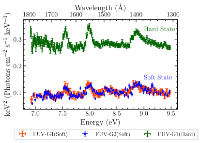
Figure 18: Hard and soft state unfolded Far-UV spectra. The models 1B (hard state) and 2D (soft state) are used for this purpose. See Sections 3.1.2 and 3.2.2 for more details.

4.3 X-ray irradiation and geometry of the outer disk

It is widely believed that the reprocessing of X-rays in the outer disk plays a dominant role in the optical/UV emission in BH-LMXBs (van Paradijs & McClintock, 1994; Gierliński et al., 2009). In the case of MAXI J1820+070, we find clear evidence of reprocessed emission in terms of excess optical/UV continuum and strong emission lines. To describe the optical/UV excess components phenomenologically, we require two low-temperature black-body components, suggesting reprocessed emission from a range of radii rather than a narrow annulus of the disk. Furthermore, we find that the multi-wavelength spectral fit with the irradiated disk model diskir provides a significantly worse fit than our phenomenological models with two low-temperature black-body components. This is perhaps not unexpected as the diskir model assumes uniform illumination of the outer accretion disk by the inner accretion flow, captured through the constant $f_{\rm out}$. In this context, we calculate the ratio of two single temperature black-body fluxes (representing UV and optical excesses, respectively) in the energy band 0.5-10.0 eV to the incoming X-ray flux in the energy band 0.1-200.0 keV in hard and soft states, and find this to be different, suggesting a non-uniform illumination of the outer accretion disk. In the hard state, the ratio of UV excess flux (0.5-10 eV) and the X-ray flux (0.1-200.0 keV) is $\sim 5.8\times 10^{-3}$, and the ratio of optical excess flux (0.5-10 eV) and the X-ray flux (0.1-200.0 keV) is $\sim 3.2\times 10^{-3}$ (Model 1C is used for this estimation). On the other hand, the same quantities in the soft state are $\sim 2\times 10^{-3}$ and $\sim 1.3\times 10^{-3}$, respectively (Model 2E is employed for this calculation). Generally, $f_{\rm out}$ should be a function of the disk aspect ratio, $H/R$ ($H$ is the disk scale-height and $R$ is the radius) and $H/R$ itself depends on $R$ (Frank et al., 2002; Meshcheryakov et al., 2018). However, in diskir, $H/R$ is assumed to be constant, which is a limiting case to the actual scenario (Meshcheryakov et al., 2018). For example, $H\propto R^{9/8}$ in the outer zone of the standard Shakura-Sunyaev model, whereas $H\propto R^{9/7}$ in isothermal disk model of Cunningham (Kimura & Done, 2019).

The observed optical/UV flux in the $0.5-10{\rm~{}eV}$ band, calculated from our multi-wavelength spectra, is $\sim 4$ and $\sim 33$ times higher than those estimated for the intrinsic disk emission in the soft and hard states using the models 2E and 1C, respectively. This clearly implies the dominance of X-ray irradiation over the intrinsic viscous dissipation in the outer disk in both soft and hard states. We find that the strength of the reprocessed optical/UV emission relative to the intrinsic disk emission is much higher in the hard state than that in the soft state. This is also evident from the stronger FUV grating spectrum in the hard state, as can be observed in Fig. 18. Also, the fraction of the intrinsic disk/corona emission reprocessed in the disk is nearly a factor of three higher in the hard state ($\sim 9\times 10^{-3}$) than in the soft state ($\sim 3.5\times 10^{-3}$). These observations clearly demonstrate that X-ray irradiation onto the disk is much more dominant in the hard state of MAXI J1820+070, similar to found in BH-LMXB XTE J1817-330 (Gierliński et al., 2009). The stronger optical and possibly UV continuum in the hard state, in principle, could also arise due to the Synchrotron emission from jets (Russell et al., 2006). The SED and timing studies of MAXI J1820+070 have shown that the jet does make a contribution to the infrared band and to the optical band to some extent (Paice et al., 2019; Markoff et al., 2020; Zdziarski et al., 2022a). However, we find that the stronger far UV continuum is accompanied by strong emission lines in the hard state. The emission lines due to He II, C IV and Si IV are nearly a factor of two stronger in the hard state than in the soft state, implying that most of the excess UV/optical emission in the hard state is due to X-ray reprocessing in the outer accretion disk. The stronger X-ray reprocessing in the hard state is most likely the outcome of the geometry where the X-ray corona in the innermost regions has larger scale height than the accretion disk, possibly in the form of a spherical corona or elongated along the jet axis. In addition, the disk wind, observed during the hard state (Muñoz-Darias et al., 2019), can also contribute to the irradiation of the disk, increasing the optical/UV flux (Gierliński et al., 2009; Dubus et al., 2019; Tetarenko et al., 2020).

We also note that it is unlikely that the emission from the secondary star is contributing a significant number of photons to the optical/UV band in both states, as the surface temperature is low, $\sim 4200$ K, i.e, $\sim 0.36$ eV (Mikołajewska et al., 2022), which is much lower than the temperature of the black-body ($\sim 0.8$ eV). However, the companion, which is detected in the optical only during quiescence, is fainter than the observed fluxes in outburst.

Finally, the high observed reprocessed fraction ($\sim 10^{-2}-10^{-3}$) from MAXI J1820+070 is unlikely to be achieved in the framework of standard thin disk prescription (Dubus et al., 1999). The outer disk is most likely convex or warped in shape, making the disk more effective for X-ray reprocessing. Interestingly, Thomas et al. (2022) proposed the outer disk of MAXI J1820+070 to be warped to explain the large amplitude modulation, seen in the hard state optical light-curves. Furthermore, a significant spin-orbit misalignment has been inferred from the optical polarimetric observations of this source (Poutanen et al., 2022), which could also result in a warped accretion disk.

5 Conclusion

Utilizing data from the AstroSat, NICER, and LCO observatories, we constrain the inner and outer geometries of the accretion flow around the BH-LMXB MAXI J1820+070 in the hard and soft states during its 2018 outburst. In the hard state, our analysis reveals that the inner accretion disk is truncated far from the ISCO radius, and has been replaced by a structured accretion flow containing two Comptonization components with different slopes and temperatures. The softer Comptonization component dominates the X-ray emission and produces broad relativistic X-ray reflection features. Meanwhile, the harder component undergoes reflection from a distant, high-density disk ($\sim 2\times 10^{20}\ \rm cm^{-3}$), resulting in unblurred reflection features. In the soft state, the X-ray spectrum features a dominant disk component (disk fraction $\sim 85\%$), a soft X-ray excess, and a weak Comptonization component. We estimate the spin of BH using continuum spectral fitting method, yielding $a=0.77\pm 0.21$, for an inclination in the range of $59^{\circ}-69^{\circ}$ (i.e., the range of jet inclination angle) and a mass in the range of $5.0-10.0M_{\sun}$ (predicted mass range of this BH). Finally, we find that a significant fraction of the X-ray radiation from the inner disk and the coronal emission is reprocessed and thermalized in the outer accretion disk, with the reprocessed fraction being much higher in the hard state ($\sim 9\times 10^{-3}$) compared to the soft state ($\sim 3.5\times 10^{-3}$). A strong reprocessing in the outer accretion disk likely suggests that the outer disk could be warped or convex, as also indicated in Thomas et al. (2022).

Table 3: Best-fit parameter values and the corresponding errors at 90$\%$ confidence level for the Model 1A (hard state). In XSPEC notation, this model reads as tbabs*constant*(diskbb+nthcomp(1)+nthcomp(2)+reflionxhd(2)+relconv*reflionxhd(1)).

Spectral Components	Parameters	Model  1A
Constant	CSXT	$1.0^{f}$
	CLAXPC	$0.736\pm 0.004$
	CCZTI-0	$0.788\pm 0.007$
	CCZTI-1	$0.796\pm 0.007$
	CCZTI-2	$0.715\pm 0.007$
	CCZTI-3	$0.771\pm 0.007$
	CNICER-1	$0.899\pm 0.002$
	CNICER-2	$0.909\pm 0.002$
tbabs	$N\rm_{H}~{}(10^{22}~{}cm^{-2})$	$0.13^{f}$
diskbb	$kT\rm_{in}$ (keV)	$0.19\pm 0.01$
	$N\rm_{\rm disk}$ ($10^{4}$)	$32.51_{-1.56}^{+1.73}$
nthcomp(1)	$\Gamma$	$1.59\pm 0.01$
	$kT\rm_{e}~{}(keV)$	$15.39\pm 0.35$
	$\rm Norm$	$4.08\pm 0.03$
nthcomp(2)	$\Gamma$	$1.17\pm 0.01$
	$kT\rm_{e}~{}(keV)$	$30.55\pm 0.97$
	$\rm Norm$	$0.15\pm 0.01$
relconv*reflionxhd(1)	$\mathcal{R}_{\rm in}$ ($R_{\rm ISCO}$)	$50.43^{+12.30}_{-9.18}$
	$q$	$3^{f}$
	$i$ (degree)	$64^{f}$
	$a$	$0.998^{f}$
	$\rm log(\rm n_{e})$	$20.31\pm 0.03$
	$\xi$	$2365.49_{-46.93}^{+64.48}$
	$A_{\rm Fe}$ ($A_{\rm Fe,solar}$)	$1.54\pm 0.04$
	$\rm Norm$	$9.14\pm 0.36$
reflionxhd(2)	$\xi$	$488.14_{-12.04}^{+13.84}$
	$\rm Norm$	$5.03\pm 0.16$
$\chi^{2}/\text{d.o.f}$		1904.2/2388

Note: In this table, $f$ means that the parameter is fixed during the fit and Norm refers to normalization. See Section 3.1.1 for more details.

Table 4: Best-fit parameter values and the corresponding errors at 90$\%$ confidence level for the Model 1B (hard state). In XSPEC, this model reads as: redden*(gauss(He II)+gauss(C IV)+gauss(Si IV)+bbodyrad(UV)).

Spectral Components	Parameters	Values
redden	$E(B-V)$	$0.17^{f}$
bbodyrad(UV)	$kT\rm_{\rm uv}$ (eV)	$3.27\pm 0.08$
	$\rm Norm$ ($10^{12}$)	$2.42_{-0.02}^{+0.09}$
gauss (Si IV)	$E$ (eV)	$8.90\pm 0.01$
	$\sigma$ ($10^{-2}$ eV)	$7.63\pm 1.26$
	$\rm Norm$	$0.45\pm 0.05$
gauss (C IV)	$E$ (eV)	$7.99\pm 0.01$
	$\sigma$ ($10^{-2}$ eV)	$1.68\pm 0.73$
	$\rm Norm$	$0.34\pm 0.04$
gauss (He II)	$E$ (eV)	$7.55\pm 0.01$
	$\sigma$ ($10^{-2}$ eV)	$1.68\pm 0.73$
	$\rm Norm$	$0.29\pm 0.04$
$\chi^{2}/\text{d.o.f}$		222.1/165

Note: In this table, $f$ means that the parameter is fixed during the fit and Norm refers to normalization. The Gaussian width ($\sigma$) of the emission lines C IV and He II are tied in this model. The component bbodyrad is normalized in the unit of $R^{2}_{\rm km}/D^{2}_{10}$, where $R_{\rm km}$ is the source radius in km. See Section 3.1.2 for more details.

Table 5: Best-fit parameter values and the corresponding errors at 90$\%$ confidence level for the Model 1C (hard state). In XSPEC, this model reads as: tbabs*redden*constant*(diskbb+nthcomp(1)+nthcomp(2)+reflionxhd(2)+relconv*reflionxhd(1)
+gauss(He II)+gauss(C IV)+gauss(Si IV)+bbodyrad(UV)+bbodyrad(optical)).

Spectral Components	Parameters	Values
Constant	CSXT	$1.0^{f}$
	CLAXPC	$0.737\pm 0.004$
	CCZTI-0	$0.789\pm 0.007$
	CCZTI-1	$0.798\pm 0.007$
	CCZTI-2	$0.717\pm 0.007$
	CCZTI-3	$0.772\pm 0.007$
	CNICER-1	$0.899\pm 0.002$
	CNICER-2	$0.909\pm 0.002$
redden	$E(B-V)$	$0.17^{f}$
tbabs	$N\rm_{H}~{}(10^{22}~{}cm^{-2})$	$0.13^{f}$
diskbb	$kT\rm_{in}$ (keV)	$0.19\pm 0.01$
	$N\rm_{\rm disk}$ ($10^{5}$)	$3.26\pm 0.18$
nthcomp(1)	$\Gamma$	$1.60\pm 0.01$
	$kT\rm_{e}~{}(keV)$	$15.37\pm 0.34$
	$\rm Norm$	$4.09\pm 0.08$
nthcomp(2)	$\Gamma$	$1.16\pm 0.01$
	$kT\rm_{e}~{}(keV)$	$30.41^{+0.84}_{+1.18}$
	$\rm Norm$	$0.14\pm 0.02$
relconv*reflionxhd(1)	$\mathcal{R}_{\rm in}$ ($R_{\rm ISCO}$)	$49.39^{+12.48}_{+8.70}$
	$i$ (degree)	$64^{f}$
	$a$	$0.998^{f}$
	$\rm log(\rm n_{e})$	$20.31\pm 0.02$
	$\xi$	$2358.39_{-45.02}^{+391.54}$
	$A_{\rm Fe}$ ($A_{\rm Fe,solar}$)	$1.56\pm 0.04$
	$\rm Norm$	$9.21\pm 0.44$
reflionxhd(2)	$\xi$	$486.02_{-09.54}^{+82.31}$
	$\rm Norm$	$4.95\pm 0.15$
bbodyrad(UV)	$kT\rm_{\rm uv}$ (eV)	$3.27^{f}$
	$\rm Norm$ ($10^{11}$)	$22.30_{-0.17}^{+0.15}$
bbodyrad(optical)	$kT\rm_{\rm optical}$ (eV)	$0.80\pm 0.03$
	$\rm Norm$ ($10^{14}$)	$1.31\pm 0.12$
gauss (Si IV)	$\rm Norm$	$0.49\pm 0.05$
gauss (C IV)	$\rm Norm$	$0.33\pm 0.04$
gauss (He II)	$\rm Norm$	$0.26\pm 0.04$
Flux (0.1-200.0 keV)		$18.87$
Flux (0.5-10.0 eV)		$0.18$
$\chi^{2}/\text{d.o.f}$		2157.7/2562

Note: In this table, $f$ means that the parameter is fixed during the fit and Norm refers to normalization. All the unabsorbed fluxes are in units of $10^{-8}\ \rm erg~{}cm^{-2}s^{-1}$. In this model, we fix $kT_{\rm uv}$, the energy and width of emission lines (described by Gaussian line profiles) at their best-fit values as found in Model 1B. See Section 3.1.3 for more details.

Table 6: Best-fit parameter values and the corresponding errors at 90$\%$ confidence level for the Models 2A, 2B, and 2C (soft state). In XSPEC notation, these models read as follows, Model 2A: tbabs*constant*thcomp*(diskbb+bbodyrad), Model 2B: tbabs*constant*thcomp*(kerrbb+bbodyrad), and Model 2C: tbabs*constant*(diskir+bbodyrad).

Spectral Components	Parameters	Model  2A	Model  2B		Model  2C
			$i$ (Free)	$i$ (Fixed)
Constant	CSXT	$1.0^{f}$	$1.0^{f}$	$1.0^{f}$	$1.0^{f}$
	CLAXPC	$1.21\pm 0.05$	$1.26\pm 0.05$	$1.25\pm 0.06$	$1.21\pm 0.06$
tbabs	$N\rm_{H}~{}(10^{20}~{}cm^{-2})$	$8.03_{-0.67}^{+0.98}$	$11.00_{-0.87}^{+0.50}$	$10.34\pm 0.86$	$8.07_{-0.71}^{+0.92}$
diskbb	$kT\rm_{in}$ (keV)	$0.58\pm 0.02$
	$N\rm_{\rm disk}$ ($10^{4}$)	$3.10_{-0.27}^{+0.50}$
bbodyrad	$kT\rm_{\rm BB}$	$0.79\pm 0.02$	$0.87\pm 0.04$	$0.84\pm 0.04$	$0.79\pm 0.02$
	$\rm Norm$ ($10^{3}$)	$2.89_{-0.49}^{+0.85}$	$0.90_{-0.22}^{+0.64}$	$1.31_{-0.53}^{+1.16}$	$2.91_{-0.53}^{+0.78}$
thcomp	$\Gamma$	$2.19\pm 0.05$	$2.15\pm 0.04$	$2.16_{-0.11}^{+0.05}$
	$kT\rm_{\rm e}~{}(keV)$	$>36.5$	$>56.2$	$>17.04$
	$cov\_frac~{}(10^{-3})$	$4.83\pm 0.99$	$3.90\pm 0.84$	$4.11\pm 0.98$
kerrbb	$M\ (\rm M_{\rm\sun})$		$9.73_{-2.52}^{+2.25}$	$8.72_{-2.82}^{+3.28p}$
	$i\ (\rm degree)$		$46.83_{-10.14}^{+4.68}$	$64^{f}$
	$a$		$0.998_{-0.157}^{+0.000p}$	$0.85_{-0.25}^{+0.10}$
	$\kappa$		$1.7^{f}$	$1.7^{f}$
	$\dot{M}$ $(10^{17}\rm g/s)$		$0.45_{-0.28}^{+0.36}$	$0.80_{-0.68}^{+11.30}$
	$\rm Norm$		$7.11_{-3.03}^{+58.31}$	$9.79_{-2.94}^{+11.07}$
diskir	$kT_{\rm disk}$ (keV)				$0.58\pm 0.02$
	$\Gamma$				$2.19\pm 0.05$
	$kT\rm_{e}~{}(keV)$				$>41.6$
	$L_{c}/L_{d}$ ($10^{-3}$)				$8.76\pm 0.76$
	$\rm Norm$ ($10^{4}$)				$3.08_{-0.29}^{+0.46}$
$\chi^{2}/\text{d.o.f}$		490.1/413	464.1/410	467.2/411	490.1/413

Note: In this table, $f$ means that the parameter is fixed during the fit, $p$ denotes that the parameter is pegged at its limit, and Norm refers to normalization. See Section 3.2.1 for more details.

Table 7: Best-fit parameter values and the corresponding errors at 90$\%$ confidence level for the Model 2D (soft state). In XSPEC, this model reads as: redden*(bbodyrad(UV)+gauss(N IV)+gauss(He II)+gauss(C IV) +gauss(N IV])+gauss(Si IV)).

Spectral Components	Parameters	Values
redden	$E(B-V)$	$0.12^{f}$
bbodyrad(UV)	$kT\rm_{\rm uv}$ (eV)	$3.87\pm 0.24$
	$\rm Norm$ ($10^{11}$)	$3.69^{+0.61}_{-0.44}$
gauss (Si IV)	$E$ (eV)	$8.88\pm 0.02$
	$\sigma$ ($10^{-2}$ eV)	$8.52\pm 1.73$
	$\rm Norm$	$0.22\pm 0.03$
gauss (N IV])	$E$ (eV)	$8.34\pm 0.02$
	$\sigma$ ($10^{-2}$ eV)	$3.19\pm 0.56$
	$\rm Norm$	$0.07\pm 0.02$
gauss (C IV)	$E$ (eV)	$7.99\pm 0.01$
	$\sigma$ ($10^{-2}$ eV)	$3.19\pm 0.56$
	$\rm Norm$	$0.16\pm 0.02$
gauss (He II)	$E$ (eV)	$7.56\pm 0.01$
	$\sigma$ ($10^{-2}$ eV)	$3.19\pm 0.56$
	$\rm Norm$	$0.13\pm 0.02$
gauss (N IV)	$E$ (eV)	$7.22\pm 0.02$
	$\sigma$ ($10^{-2}$ eV)	$3.19\pm 0.56$
	$\rm Norm$	$0.08\pm 0.02$
$\chi^{2}/\text{d.o.f}$		408.6/333

Note: In this table, $f$ means that the parameter is fixed during the fit and Norm refers to normalization. The Gaussian width ($\sigma$) of the emission lines N IV], C IV, He II, and N IV are tied in this model. See Section 3.2.2 for more details.

Table 8: Best-fit parameter values and the corresponding errors at 90$\%$ confidence level for the Models 2E, 2F, and 2G (soft state). In XSPEC notation, these models read as follows, Model 2E: tbabs*redden*con*(bbodyrad(UV)+bbodyrad(optical)+gauss(N IV)+gauss(He II)+gauss(C IV)+gauss(N IV])+gauss(Si IV)+thcomp*(bbodyrad+diskbb)), Model 2F: tbabs*redden*con*(bbodyrad(UV)+bbodyrad(optical)+gauss(N IV)+gauss(He II)+gauss(C IV)+gauss(N IV])+gauss(Si IV)+thcomp*(bbodyrad+kerrbb)), and Model 2G: tbabs*redden*con*(gauss(He II)+gauss(C IV)+gauss(N IV])+gauss(Si IV)+bbodyrad+diskir).

Spectral Components	Parameters	Model  2E	Model  2F	Model  2G
Constant	CSXT	$1.0^{f}$	$1.0^{f}$	$1.0^{f}$
	CLAXPC	$1.18\pm 0.05$	$1.28\pm 0.05$	$1.18\pm 0.03$
tbabs	$N\rm_{H}~{}(10^{20}~{}cm^{-2})$	$9.0^{f}$	$9.0^{f}$	$9.0^{f}$
redden	$E(B-V)$	$0.12^{f}$	$0.12^{f}$	$0.12^{f}$
bbodyrad	$kT\rm_{\rm BB}$	$0.79\pm 0.01$	$0.89\pm 0.03$	$0.79\pm 0.01$
	$\rm Norm~{}(10^{3})$	$3.41_{-0.39}^{+0.57}$	$0.68_{-0.28}^{+0.35}$	$3.35_{-0.20}^{+0.40}$
diskbb	$kT\rm_{\rm in}$	$0.56\pm 0.01$
	$N\rm_{\rm disk}$ ($10^{4}$)	$3.49_{-0.18}^{+0.26}$
thcomp	$\Gamma$	$2.20\pm 0.05$	$2.14_{-0.15}^{+0.05}$
	$kT\rm_{\rm e}~{}(keV)$	$>40.96$	$>17.42$
	$\rm cov\_frac$ ($10^{-3}$)	$5.02\pm 0.92$	$3.86\pm 1.01$
kerrbb	$M\ (\rm M_{\rm\sun})$		$6.75^{f}$
	$i\ (\rm degree)$		$64^{f}$
	$a$		$0.75^{f}$
	$\kappa$		$1.7^{f}$
	$\dot{M}$ $(10^{17}\rm g/s)$		$1.48_{-0.09}^{+0.13}$
	$\rm Norm$		$8.68\pm 0.57$
diskir	$kT_{\rm disk}$ (keV)			$0.57\pm 0.01$
	$\Gamma$			$2.20\pm 0.04$
	$kT\rm_{e}~{}(keV)$			$>45.3$
	$L_{c}/L_{d}$ ($10^{-3}$)			$9.11\pm 0.56$
	$f_{\rm out}$ ($10^{-3}$)			$1.98\pm 0.03$
	$\rm log(r_{\rm out})$			$4.38\pm 0.02$
	$\rm Norm$ ($10^{4}$)			$3.42_{-0.10}^{+0.19}$
bbodyrad(UV)	$kT\rm_{\rm uv}$ (eV)	$3.87^{f}$	$3.87^{f}$
	$\rm Norm$ ($10^{11}$)	$2.55_{-0.05}^{+0.04}$	$2.32\pm 0.05$
bbodyrad(optical)	$kT\rm_{\rm optical}$ (eV)	$0.75\pm 0.04$	$0.75\pm 0.04$
	$\rm Norm$ ($10^{13}$)	$3.51_{-0.50}^{+0.55}$	$3.35_{-0.50}^{+0.56}$
gauss (Si IV)	$\rm Norm$	$0.25\pm 0.03$	$0.26\pm 0.03$	$0.38\pm 0.03$
gauss (N IV])	$\rm Norm$	$0.09\pm 0.02$	$0.09\pm 0.02$	$0.11\pm 0.02$
gauss (C IV)	$\rm Norm$	$0.18\pm 0.02$	$0.18\pm 0.02$	$0.16\pm 0.02$
gauss (He II)	$\rm Norm$	$0.14\pm 0.02$	$0.14\pm 0.02$	$0.09\pm 0.02$
gauss (N IV)	$\rm Norm$	$0.07\pm 0.03$	$0.07\pm 0.03$
Flux (0.1-200.0 keV)		10.50	11.53	10.56
Flux (0.5-10.0 eV)		0.049	0.053	0.056
$\chi^{2}/\text{d.o.f}$		900.5/756	881.9/756	1230.6/758

Note: In this table, Norm refers to the normalization of the associated spectral component, $f$ means that the parameter is fixed during the fit, and $p$ denotes that the parameter is pegged at its limit. All the unabsorbed fluxes are in units of $10^{-8}\ \rm erg~{}cm^{-2}s^{-1}$. In this model, we fix $kT_{\rm uv}$, the energy and width of emission lines (described by Gaussian line profiles) at their best-fit values as found in Model 2D. See Section 3.2.3 for more details.

References

- Antia et al. (2017) Antia, H. M., Yadav, J. S., Agrawal, P. C., et al. 2017, The Astrophysical Journal Supplement Series, 231, 10, doi: 10.3847/1538-4365/aa7a0e
- Antia et al. (2021) Antia, H. M., Agrawal, P. C., Dedhia, D., et al. 2021, Journal of Astrophysics and Astronomy, 42, 32, doi: 10.1007/s12036-021-09712-8
- Arnaud (1996) Arnaud, K. A. 1996, in Astronomical Society of the Pacific Conference Series, Vol. 101, Astronomical Data Analysis Software and Systems V, ed. G. H. Jacoby & J. Barnes, 17
- Atri et al. (2020) Atri, P., Miller-Jones, J. C. A., Bahramian, A., et al. 2020, MNRAS, 493, L81, doi: 10.1093/mnrasl/slaa010
- Axelsson & Veledina (2021) Axelsson, M., & Veledina, A. 2021, MNRAS, 507, 2744, doi: 10.1093/mnras/stab2191
- Baglio et al. (2018) Baglio, M. C., Russell, D. M., & Lewis, F. 2018, The Astronomer’s Telegram, 11418, 1
- Bahramian et al. (2018) Bahramian, A., Strader, J., & Dage, K. 2018, The Astronomer’s Telegram, 11424, 1
- Banerjee et al. (2019a) Banerjee, S., Chakraborty, C., & Bhattacharyya, S. 2019a, ApJ, 870, 95, doi: 10.3847/1538-4357/aaf102
- Banerjee et al. (2019b) —. 2019b, MNRAS, 487, 3488, doi: 10.1093/mnras/stz1518
- Banerjee et al. (2020) Banerjee, S., Gilfanov, M., Bhattacharyya, S., & Sunyaev, R. 2020, MNRAS, 498, 5353, doi: 10.1093/mnras/staa2788
- Basak & Zdziarski (2016) Basak, R., & Zdziarski, A. A. 2016, MNRAS, 458, 2199, doi: 10.1093/mnras/stw420
- Belloni (2010) Belloni, T. M. 2010, in Lecture Notes in Physics, Berlin Springer Verlag, ed. T. Belloni, Vol. 794, 53, doi: 10.1007/978-3-540-76937-8_3
- Belloni & Motta (2016) Belloni, T. M., & Motta, S. E. 2016, in Astrophysics and Space Science Library, Vol. 440, Astrophysics of Black Holes: From Fundamental Aspects to Latest Developments, ed. C. Bambi, 61, doi: 10.1007/978-3-662-52859-4_2
- Bhalerao et al. (2017) Bhalerao, V., Bhattacharya, D., Vibhute, A., et al. 2017, Journal of Astrophysics and Astronomy, 38, 31, doi: 10.1007/s12036-017-9447-8
- Bhargava et al. (2021) Bhargava, Y., Belloni, T., Bhattacharya, D., Motta, S., & Ponti., G. 2021, MNRAS, 508, 3104, doi: 10.1093/mnras/stab2848
- Bright et al. (2018) Bright, J., Fender, R., & Motta, S. 2018, The Astronomer’s Telegram, 11420, 1
- Bright et al. (2020) Bright, J. S., Fender, R. P., Motta, S. E., et al. 2020, Nature Astronomy, 4, 697, doi: 10.1038/s41550-020-1023-5
- Buisson et al. (2019) Buisson, D. J. K., Fabian, A. C., Barret, D., et al. 2019, MNRAS, 490, 1350, doi: 10.1093/mnras/stz2681
- Casella et al. (2018) Casella, P., Vincentelli, F., O’Brien, K., et al. 2018, The Astronomer’s Telegram, 11451, 1
- Chakraborty et al. (2020) Chakraborty, S., Navale, N., Ratheesh, A., & Bhattacharyya, S. 2020, MNRAS, 498, 5873, doi: 10.1093/mnras/staa2711
- Chakraborty et al. (2021) Chakraborty, S., Ratheesh, A., Bhattacharyya, S., et al. 2021, MNRAS, 508, 475, doi: 10.1093/mnras/stab2530
- Connors et al. (2021) Connors, R. M. T., García, J. A., Tomsick, J., et al. 2021, ApJ, 909, 146, doi: 10.3847/1538-4357/abdd2c
- Dauser et al. (2014) Dauser, T., Garcia, J., Parker, M. L., Fabian, A. C., & Wilms, J. 2014, MNRAS, 444, L100, doi: 10.1093/mnrasl/slu125
- Dauser et al. (2016) Dauser, T., García, J., Walton, D. J., et al. 2016, A&A, 590, A76, doi: 10.1051/0004-6361/201628135
- Dauser et al. (2010) Dauser, T., Wilms, J., Reynolds, C. S., & Brenneman, L. W. 2010, MNRAS, 409, 1534, doi: 10.1111/j.1365-2966.2010.17393.x
- De Marco et al. (2021) De Marco, B., Zdziarski, A. A., Ponti, G., et al. 2021, A&A, 654, A14, doi: 10.1051/0004-6361/202140567
- Denisenko (2018) Denisenko, D. 2018, The Astronomer’s Telegram, 11400, 1
- Dewangan (2021) Dewangan, G. C. 2021, Journal of Astrophysics and Astronomy, 42, 49, doi: 10.1007/s12036-021-09691-w
- Done et al. (2007) Done, C., Gierliński, M., & Kubota, A. 2007, A&A Rev., 15, 1, doi: 10.1007/s00159-007-0006-1
- Dubus et al. (2019) Dubus, G., Done, C., Tetarenko, B. E., & Hameury, J.-M. 2019, A&A, 632, A40, doi: 10.1051/0004-6361/201936333
- Dubus et al. (1999) Dubus, G., Lasota, J.-P., Hameury, J.-M., & Charles, P. 1999, MNRAS, 303, 139, doi: 10.1046/j.1365-8711.1999.02212.x
- Dziełak et al. (2021) Dziełak, M. A., De Marco, B., & Zdziarski, A. A. 2021, Monthly Notices of the Royal Astronomical Society, 506, 2020, doi: 10.1093/mnras/stab1700
- Echiburú-Trujillo et al. (2023) Echiburú-Trujillo, C., Tetarenko, A. J., Haggard, D., et al. 2023, arXiv e-prints, arXiv:2311.11523, doi: 10.48550/arXiv.2311.11523
- Fabian (2005) Fabian, A. C. 2005, Broad iron lines in AGN and X-ray binaries, ed. T. J. Maccarone, R. P. Fender, & L. C. Ho (Dordrecht: Springer Netherlands), 97–105, doi: 10.1007/1-4020-4085-7_12
- Fabian et al. (1989) Fabian, A. C., Rees, M. J., Stella, L., & White, N. E. 1989, MNRAS, 238, 729, doi: 10.1093/mnras/238.3.729
- Fabian et al. (2020) Fabian, A. C., Buisson, D. J., Kosec, P., et al. 2020, MNRAS, 493, 5389, doi: 10.1093/mnras/staa564
- Frank et al. (2002) Frank, J., King, A., & Raine, D. J. 2002, Accretion Power in Astrophysics: Third Edition
- Fürst et al. (2015) Fürst, F., Nowak, M. A., Tomsick, J. A., et al. 2015, ApJ, 808, 122, doi: 10.1088/0004-637X/808/2/122
- Gandhi et al. (2018) Gandhi, P., Paice, J. A., Littlefair, S. P., et al. 2018, The Astronomer’s Telegram, 11437, 1
- García et al. (2013) García, J., Dauser, T., Reynolds, C. S., et al. 2013, ApJ, 768, 146, doi: 10.1088/0004-637X/768/2/146
- García et al. (2014) García, J., Dauser, T., Lohfink, A., et al. 2014, ApJ, 782, 76, doi: 10.1088/0004-637X/782/2/76
- García et al. (2015) García, J. A., Dauser, T., Steiner, J. F., et al. 2015, ApJ, 808, L37, doi: 10.1088/2041-8205/808/2/L37
- García et al. (2016) García, J. A., Fabian, A. C., Kallman, T. R., et al. 2016, MNRAS, 462, 751, doi: 10.1093/mnras/stw1696
- Gendreau et al. (2016) Gendreau, K. C., Arzoumanian, Z., Adkins, P. W., et al. 2016, in Space Telescopes and Instrumentation 2016: Ultraviolet to Gamma Ray, ed. J.-W. A. den Herder, T. Takahashi, & M. Bautz, Vol. 9905, International Society for Optics and Photonics (SPIE), 420 – 435, doi: 10.1117/12.2231304
- Gierliński et al. (2009) Gierliński, M., Done, C., & Page, K. 2009, MNRAS, 392, 1106, doi: 10.1111/j.1365-2966.2008.14166.x
- Gilfanov (2010) Gilfanov, M. 2010, in Lecture Notes in Physics, Berlin Springer Verlag, ed. T. Belloni, Vol. 794, 17, doi: 10.1007/978-3-540-76937-8_2
- Gilfanov & Arefiev (2005) Gilfanov, M., & Arefiev, V. 2005, arXiv e-prints, astro, doi: 10.48550/arXiv.astro-ph/0501215
- Haardt & Maraschi (1991) Haardt, F., & Maraschi, L. 1991, ApJ, 380, L51, doi: 10.1086/186171
- Harris et al. (2016) Harris, D. W., Jensen, T. W., Suzuki, N., et al. 2016, AJ, 151, 155, doi: 10.3847/0004-6256/151/6/155
- HI4PI Collaboration et al. (2016) HI4PI Collaboration, Ben Bekhti, N., Flöer, L., et al. 2016, A&A, 594, A116, doi: 10.1051/0004-6361/201629178
- Homan & Belloni (2005) Homan, J., & Belloni, T. 2005, Ap&SS, 300, 107, doi: 10.1007/s10509-005-1197-4
- Homan et al. (2001) Homan, J., Wijnands, R., van der Klis, M., et al. 2001, ApJS, 132, 377, doi: 10.1086/318954
- Homan et al. (2018) Homan, J., Stevens, A. L., Altamirano, D., et al. 2018, The Astronomer’s Telegram, 12068, 1
- Homan et al. (2020) Homan, J., Bright, J., Motta, S. E., et al. 2020, ApJ, 891, L29, doi: 10.3847/2041-8213/ab7932
- Jiang et al. (2020) Jiang, J., Gallo, L. C., Fabian, A. C., Parker, M. L., & Reynolds, C. S. 2020, MNRAS, 498, 3888, doi: 10.1093/mnras/staa2625
- Kaastra & Bleeker (2016) Kaastra, J. S., & Bleeker, J. A. M. 2016, A&A, 587, A151, doi: 10.1051/0004-6361/201527395
- Kajava et al. (2019) Kajava, J. J. E., Motta, S. E., Sanna, A., et al. 2019, MNRAS, 488, L18, doi: 10.1093/mnrasl/slz089
- Kara et al. (2019) Kara, E., Steiner, J. F., Fabian, A. C., et al. 2019, Nature, 565, 198, doi: 10.1038/s41586-018-0803-x
- Kawamuro et al. (2018) Kawamuro, T., Negoro, H., Yoneyama, T., et al. 2018, The Astronomer’s Telegram, 11399, 1
- Kimura & Done (2019) Kimura, M., & Done, C. 2019, MNRAS, 482, 626, doi: 10.1093/mnras/sty2736
- Kubota et al. (1998) Kubota, A., Tanaka, Y., Makishima, K., et al. 1998, PASJ, 50, 667, doi: 10.1093/pasj/50.6.667
- Kumar et al. (2023) Kumar, S., Dewangan, G. C., Singh, K. P., et al. 2023, ApJ, 950, 90, doi: 10.3847/1538-4357/acc941
- Lewis (2018) Lewis, F. 2018, Robotic Telescope, Student Research and Education Proceedings, 1, 237, doi: 10.48550/arXiv.1807.00762
- Li et al. (2005) Li, L.-X., Zimmerman, E. R., Narayan, R., & McClintock, J. E. 2005, ApJS, 157, 335, doi: 10.1086/428089
- Liska et al. (2018) Liska, M., Hesp, C., Tchekhovskoy, A., et al. 2018, MNRAS, 474, L81, doi: 10.1093/mnrasl/slx174
- Littlefield (2018) Littlefield, C. 2018, The Astronomer’s Telegram, 11421, 1
- Makishima et al. (1986) Makishima, K., Maejima, Y., Mitsuda, K., et al. 1986, ApJ, 308, 635, doi: 10.1086/164534
- Mandal et al. (2018) Mandal, A. K., Singh, A., Stalin, C. S., Chandra, S., & Gandhi, P. 2018, The Astronomer’s Telegram, 11458, 1
- Marino et al. (2021) Marino, A., Barnier, S., Petrucci, P. O., et al. 2021, A&A, 656, A63, doi: 10.1051/0004-6361/202141146
- Markoff et al. (2020) Markoff, S., Russell, D. M., Dexter, J., et al. 2020, MNRAS, 495, 525, doi: 10.1093/mnras/staa1193
- McClintock et al. (2014) McClintock, J. E., Narayan, R., & Steiner, J. F. 2014, Space Sci. Rev., 183, 295, doi: 10.1007/s11214-013-0003-9
- Meshcheryakov et al. (2018) Meshcheryakov, A. V., Tsygankov, S. S., Khamitov, I. M., et al. 2018, MNRAS, 473, 3987, doi: 10.1093/mnras/stx2565
- Mikołajewska et al. (2022) Mikołajewska, J., Zdziarski, A. A., Ziółkowski, J., Torres, M. A. P., & Casares, J. 2022, ApJ, 930, 9, doi: 10.3847/1538-4357/ac6099
- Mitsuda et al. (1984) Mitsuda, K., Inoue, H., Koyama, K., et al. 1984, PASJ, 36, 741
- Morton (2003) Morton, D. C. 2003, ApJS, 149, 205, doi: 10.1086/377639
- Muñoz-Darias et al. (2019) Muñoz-Darias, T., Jiménez-Ibarra, F., Panizo-Espinar, G., et al. 2019, ApJ, 879, L4, doi: 10.3847/2041-8213/ab2768
- Özbey Arabacı et al. (2022) Özbey Arabacı, M., Kalemci, E., Dinçer, T., et al. 2022, MNRAS, 514, 3894, doi: 10.1093/mnras/stac1574
- Paice et al. (2019) Paice, J. A., Gandhi, P., Shahbaz, T., et al. 2019, MNRAS, 490, L62, doi: 10.1093/mnrasl/slz148
- Pirbhoy et al. (2020) Pirbhoy, S. F., Baglio, M. C., Russell, D. M., et al. 2020, The Astronomer’s Telegram, 13451, 1
- Postma & Leahy (2017) Postma, J. E., & Leahy, D. 2017, Publications of the Astronomical Society of the Pacific, 129, 115002, doi: 10.1088/1538-3873/aa8800
- Poutanen et al. (2018) Poutanen, J., Veledina, A., & Zdziarski, A. A. 2018, A&A, 614, A79, doi: 10.1051/0004-6361/201732345
- Poutanen et al. (2022) Poutanen, J., Veledina, A., Berdyugin, A. V., et al. 2022, Science, 375, 874, doi: 10.1126/science.abl4679
- Reis et al. (2010) Reis, R. C., Fabian, A. C., & Miller, J. M. 2010, MNRAS, 402, 836, doi: 10.1111/j.1365-2966.2009.15976.x
- Reis et al. (2009) Reis, R. C., Miller, J. M., & Fabian, A. C. 2009, MNRAS, 395, L52, doi: 10.1111/j.1745-3933.2009.00640.x
- Remillard & McClintock (2006) Remillard, R. A., & McClintock, J. E. 2006, ARA&A, 44, 49, doi: 10.1146/annurev.astro.44.051905.092532
- Remillard et al. (2021) Remillard, R. A., Loewenstein, M., Steiner, J. F., et al. 2021, arXiv e-prints, arXiv:2105.09901. https://arxiv.org/abs/2105.09901
- Rodi et al. (2021) Rodi, J., Tramacere, A., Onori, F., et al. 2021, ApJ, 910, 21, doi: 10.3847/1538-4357/abdfd0
- Ross & Fabian (2005) Ross, R. R., & Fabian, A. C. 2005, MNRAS, 358, 211, doi: 10.1111/j.1365-2966.2005.08797.x
- Ross & Fabian (2007) —. 2007, MNRAS, 381, 1697, doi: 10.1111/j.1365-2966.2007.12339.x
- Russell et al. (2019a) Russell, D. M., Baglio, M. C., & Lewis, F. 2019a, The Astronomer’s Telegram, 12534, 1
- Russell et al. (2006) Russell, D. M., Fender, R. P., Hynes, R. I., et al. 2006, MNRAS, 371, 1334, doi: 10.1111/j.1365-2966.2006.10756.x
- Russell et al. (2019b) Russell, D. M., Bramich, D. M., Lewis, F., et al. 2019b, Astronomische Nachrichten, 340, 278, doi: 10.1002/asna.201913610
- Sako et al. (2018) Sako, S., Ohsawa, R., Ichiki, M., et al. 2018, The Astronomer’s Telegram, 11426, 1
- Shakura & Sunyaev (1973) Shakura, N. I., & Sunyaev, R. A. 1973, A&A, 24, 337
- Shidatsu et al. (2019) Shidatsu, M., Nakahira, S., Murata, K. L., et al. 2019, ApJ, 874, 183, doi: 10.3847/1538-4357/ab09ff
- Shimura & Takahara (1995) Shimura, T., & Takahara, F. 1995, ApJ, 445, 780, doi: 10.1086/175740
- Singh et al. (2017) Singh, K., Stewart, G., Westergaard, N., et al. 2017, Journal of Astrophysics and Astronomy, 38, 1
- Singh et al. (2014) Singh, K. P., Tandon, S. N., Agrawal, P. C., et al. 2014, in Space Telescopes and Instrumentation 2014: Ultraviolet to Gamma Ray, ed. T. Takahashi, J.-W. A. den Herder, & M. Bautz, Vol. 9144, International Society for Optics and Photonics (SPIE), 517 – 531, doi: 10.1117/12.2062667
- Singh et al. (2016) Singh, K. P., Stewart, G. C., Chandra, S., et al. 2016, in Space Telescopes and Instrumentation 2016: Ultraviolet to Gamma Ray, Vol. 9905, International Society for Optics and Photonics, 99051E
- Sunyaev & Titarchuk (1980) Sunyaev, R. A., & Titarchuk, L. G. 1980, A&A, 86, 121
- Tandon et al. (2017) Tandon, S., Subramaniam, A., Girish, V., et al. 2017, The Astronomical Journal, 154, 128
- Tandon et al. (2020) Tandon, S., Postma, J., Joseph, P., et al. 2020, The Astronomical Journal, 159, 158
- Tetarenko et al. (2020) Tetarenko, B. E., Dubus, G., Marcel, G., Done, C., & Clavel, M. 2020, MNRAS, 495, 3666, doi: 10.1093/mnras/staa1367
- Thomas et al. (2022) Thomas, J. K., Charles, P. A., Buckley, D. A. H., et al. 2022, MNRAS, 509, 1062, doi: 10.1093/mnras/stab3033
- Tomsick et al. (2018) Tomsick, J. A., Parker, M. L., García, J. A., et al. 2018, ApJ, 855, 3, doi: 10.3847/1538-4357/aaaab1
- Tonry et al. (2018) Tonry, J. L., Denneau, L., Flewelling, H., et al. 2018, ApJ, 867, 105, doi: 10.3847/1538-4357/aae386
- Torres et al. (2020) Torres, M. A. P., Casares, J., Jiménez-Ibarra, F., et al. 2020, ApJ, 893, L37, doi: 10.3847/2041-8213/ab863a
- Torres et al. (2019) —. 2019, ApJ, 882, L21, doi: 10.3847/2041-8213/ab39df
- Trushkin et al. (2018) Trushkin, S. A., Nizhelskij, N. A., Tsybulev, P. G., & Erkenov, A. 2018, The Astronomer’s Telegram, 11439, 1
- Uttley et al. (2018) Uttley, P., Gendreau, K., Markwardt, C., et al. 2018, The Astronomer’s Telegram, 11423, 1
- Vadawale et al. (2016) Vadawale, S. V., Rao, A. R., Bhattacharya, D., et al. 2016, SPIE Proceedings, 9905, 409, doi: 10.1117/12.2235373
- van Paradijs & McClintock (1994) van Paradijs, J., & McClintock, J. E. 1994, A&A, 290, 133
- Vanden Berk et al. (2001) Vanden Berk, D. E., Richards, G. T., Bauer, A., et al. 2001, AJ, 122, 549, doi: 10.1086/321167
- Verner et al. (1996) Verner, D. A., Ferland, G. J., Korista, K. T., & Yakovlev, D. G. 1996, ApJ, 465, 487, doi: 10.1086/177435
- Wang et al. (2020) Wang, Y., Ji, L., Zhang, S. N., et al. 2020, The Astrophysical Journal, 896, 33, doi: 10.3847/1538-4357/ab8db4
- Weisskopf et al. (2010) Weisskopf, M. C., Guainazzi, M., Jahoda, K., et al. 2010, ApJ, 713, 912, doi: 10.1088/0004-637X/713/2/912
- Wilms et al. (2000) Wilms, J., Allen, A., & McCray, R. 2000, ApJ, 542, 914, doi: 10.1086/317016
- Wood et al. (2021) Wood, C. M., Miller-Jones, J. C. A., Homan, J., et al. 2021, MNRAS, 505, 3393, doi: 10.1093/mnras/stab1479
- Yadav et al. (2016) Yadav, J., Agrawal, P., Antia, H., et al. 2016, in Space Telescopes and Instrumentation 2016: Ultraviolet to Gamma Ray, Vol. 9905, SPIE, 374–388
- Zdziarski & De Marco (2020) Zdziarski, A. A., & De Marco, B. 2020, ApJ, 896, L36, doi: 10.3847/2041-8213/ab9899
- Zdziarski et al. (2021a) Zdziarski, A. A., Dziełak, M. A., De Marco, B., Szanecki, M., & Niedźwiecki, A. 2021a, ApJ, 909, L9, doi: 10.3847/2041-8213/abe7ef
- Zdziarski et al. (1996) Zdziarski, A. A., Johnson, W. N., & Magdziarz, P. 1996, MNRAS, 283, 193, doi: 10.1093/mnras/283.1.193
- Zdziarski et al. (2020) Zdziarski, A. A., Szanecki, M., Poutanen, J., Gierliński, M., & Biernacki, P. 2020, MNRAS, 492, 5234, doi: 10.1093/mnras/staa159
- Zdziarski et al. (2022a) Zdziarski, A. A., Tetarenko, A. J., & Sikora, M. 2022a, ApJ, 925, 189, doi: 10.3847/1538-4357/ac38a9
- Zdziarski et al. (2022b) Zdziarski, A. A., You, B., Szanecki, M., Li, X.-B., & Ge, M. 2022b, ApJ, 928, 11, doi: 10.3847/1538-4357/ac54a7
- Zdziarski et al. (2021b) Zdziarski, A. A., Jourdain, E., Lubiński, P., et al. 2021b, ApJ, 914, L5, doi: 10.3847/2041-8213/ac0147
- Zhang et al. (2020) Zhang, L., Altamirano, D., Cúneo, V. A., et al. 2020, MNRAS, 499, 851, doi: 10.1093/mnras/staa2842
- Zhao et al. (2021) Zhao, X., Gou, L., Dong, Y., et al. 2021, ApJ, 916, 108, doi: 10.3847/1538-4357/ac07a9
- Zhu et al. (2017) Zhu, H., Tian, W., Li, A., & Zhang, M. 2017, MNRAS, 471, 3494, doi: 10.1093/mnras/stx1580
- Życki et al. (1999) Życki, P. T., Done, C., & Smith, D. A. 1999, MNRAS, 309, 561, doi: 10.1046/j.1365-8711.1999.02885.x