Color Image Denoising Using The Green Channel Prior

Abstract

Noise removal in the standard RGB (sRGB) space remains a challenging task, in that the noise statistics of real-world images can be different in R, G and B channels. In fact, the green channel usually has twice the sampling rate in raw data and a higher signal-to-noise ratio than red/blue ones. However, the green channel prior (GCP) is often understated or ignored in color image denoising since many existing approaches mainly focus on modeling the relationship among image patches. In this paper, we propose a simple and effective one step GCP-based image denoising (GCP-ID) method, which aims to exploit the GCP for denoising in the sRGB space by integrating it into the classic nonlocal transform domain denoising framework. Briefly, we first take advantage of the green channel to guide the search of similar patches, which improves the patch search quality and encourages sparsity in the transform domain. Then we reformulate RGB patches into RGGB arrays to explicitly characterize the density of green samples. The block circulant representation is utilized to capture the cross-channel correlation and the channel redundancy. Experiments on both synthetic and real-world datasets demonstrate the competitive performance of the proposed GCP-ID method for the color image and video denoising tasks. The code is available at github.com/ZhaomingKong/GCP-ID.

1 Introduction

The rapid development of digital cameras has largely facilitated the recording of colorful and dynamic objects, preserving and presenting rich information of real scenes. Inevitably, image data are contaminated by noise to varying degrees during acquisition and transmission. Therefore image denoising plays an indispensable role in modern imaging systems. Meanwhile the growth in the number and size of images also poses a greater demand on noise removal in terms of both effectiveness and efficiency.
The target of noise removal is to recover a clean image $\mathcal{X}$ from its noisy observation $\mathcal{Y}=\mathcal{X}+\mathcal{N}$, where $\mathcal{N}$ is usually modeled as additive white Gaussian noise (AWGN) with standard deviation (std) $\sigma$. Image denoising enjoys a long history and early works focus on handling single-channel images [buades2005review, aharon2006k, zoran2011learning]. When the input is an RGB image, naively filtering each channel separately will lead to unsatisfactory results since the spectral correlation among RGB channels is ignored [xu2017multi]. To improve the channel-by-channel algorithm, two solutions are mainly adopted. The first strategy is to apply a decorrelation transform along the RGB dimension, and then handle each channel of the transformed space independently. For example, the representative CBM3D method [dabov2007color] considers the luminance-chrominance (e.g., YCbCr) space as a less correlated color space. An alternative strategy is to jointly denoise RGB channels simultaneously by concatenating RGB patches, and applying traditional transforms such as singular value decomposition (SVD) [xu2017multi, jha2010denoising] and wavelet filters [tian2023multi, ruikar2011wavelet] or deep neural networks (DNNs) such as convolution neural networks (CNNs) [zhang2017beyond, zhang2018ffdnet] and transformers [zamir2022restormer, liang2021swinir].
Despite the outstanding performance of existing methods, they are restricted to directly treating RGB patch as a whole or assigning different weights to each channel. In addition, the main focus of many related works lies in the modeling of relationship among image patches by imposing various regularization terms and solving complex optimization problems [chang2017hyper, mahdaoui2022image], which may drastically increase computational burden and fail to exploit the difference of noise statistics in RGB channels. It is noticed that to reconstruct a full-resolution color image from sensor readings, a digital camera generally goes through the image demosaicing process [menon2011color] based on the Bayer color filter array (CFA) pattern [chung2008lossless], which measures the green channel at a higher sampling rate than red/blue ones. Such prior knowledge is known as the green channel prior (GCP), however the GCP is commonly used in processing and applications of raw sensor data [liu2020joint, guo2021joint, zhang2022joint], which are not always available. Therefore, it is interesting to investigate if the GCP can be leveraged to guide denoising in the sRGB space.
Motivated by the fact that the green channel has a higher signal-to-noise ratio (SNR) than red/blue ones in most natural images, in this paper, we present a GCP-based image denoising (GCP-ID) method for color images. The proposed GCP-ID follows the traditional nonlocal transform domain framework due to its simplicity, effectiveness and adaptiveness [kong2023comparison, elad2023image]. The performance of traditional patch-based denoisers is often affected by two decisive factors: nonlocal similar patch search and proper representation for local image patches. To improve the classic paradigm, GCP-ID utilizes the green channel to guide the search of similar patches because the green channel is less noisier and preserves better image structure and details. Then the similar patches are stacked into a group and the group-level relationship can be captured by performing principal component analysis (PCA) along the grouping dimension [dabov2009bm3d, zhang2010two]. In order to model the density of green samples and the importance of the green channel, each RGB image patch is reformulated into RGGB array based on the Bayer pattern. The spectral correlation among RGB channels is further exploited with block circulant representation. Eventually, the patch-level redundancy can be characterized by the tensor-SVD (t-SVD) transform [kilmer2011factorization, kilmer2013third]. Our contributions can ne summarized as follows:

• To explicitly take advantage of the GCP for sRGB data, we present a novel denoiser GCP-ID by integrating it into the classic patch-based denoising framework.

• We propose to reformulate image patches as RGGB arrays and utilize block circulant representation to capture their spectral correlation. The formulation is simplified as a one step t-SVD transform.

• Experiments demonstrate the competitive performance of GCP-ID for both real-world color image and video denoising tasks. Besides, we study how the GCP may be extended to other imaging techniques such as Multispectral/Hyperspectral imaging (MSI/HSI).

2 Notations and Preliminaries

In this paper, vectors and matrices are denoted by boldface lowercase letters $\mathbf{a}$ and capital letters $\mathbf{A}$, respectively. Tensors [kolda2009tensor] are denoted by calligraphic letters, e.g., $\mathcal{A}$. Given an $N$th-order tensor $\mathcal{A}\in\mathbb{R}^{I_{1}\times I_{2}\times\cdots\times I_{N}}$, the Frobenius norm of a tensor $\mathcal{A}\in\mathbb{R}^{I_{1}\times I_{2}\times\cdots\times I_{N}}$ is defined as $\|\mathcal{A}\|_{F}=\sqrt{\sum_{i_{1}=1}...\sum_{i_{N}=1}\mathcal{A}_{i_{1}...i_{N}}^{2}}$. The $n$-mode product of a tensor $\mathcal{A}$ by a matrix $\mathbf{U}\in\mathrm{R}^{P_{n}\times I_{n}}$ is denoted by $\mathcal{A}\times_{n}\mathbf{U}\in\mathbb{R}^{I_{1}\cdots I_{n-1}P_{n}I_{n+1}\cdots I_{N}}$.
The product between matrices can be generalized to the product of two tensors according to t-product [kilmer2013third]. Specifically, the t-product ‘$*$’ between two third-order tensors $\mathcal{A}\in\mathbb{R}^{N_{1}\times N_{2}\times N_{3}}$ and $\mathcal{B}\in\mathbb{R}^{N_{1}\times N_{4}\times N_{3}}$ is also a third order tensor $\mathcal{C}\in\mathbb{R}^{N_{1}\times N_{4}\times N_{3}}$ with $\mathcal{C}=\mathcal{A}*\mathcal{B}$ computed by

$$bcirc(\mathcal{C})=bcirc(\mathcal{A})bcirc(\mathcal{B})$$ (1)

where $bcirc$ is the block circulant operation that reshapes a third order tensor into a block circulant matrix [kilmer2013third]. Directly handling block circulant matrices is time consuming. Eq. (1) can be computed efficiently in the Fourier domain

$$bdiag(\mathcal{C}_{FFT})=bdiag(\mathcal{A}_{F})bdiag(\mathcal{B}_{F})$$ (2)

where $bdiag$ is the block diagonal representation, $\mathcal{A}_{F}$ is obtained by performing the fast Fourier transform (FFT) along the third mode of $\mathcal{A}$ via $\mathcal{A}_{F}=\mathcal{A}\times_{3}\mathbf{W}_{FFT}$, and $\mathbf{W}_{FFT}$ is the fast Fourier transform (FFT) matrix.
The tensor-SVD or t-SVD of a third-order tensor can then be defined as the t-product of three third-order tensors

$$\mathcal{A}=\mathcal{U}*\mathcal{S}*\mathcal{V}^{T}$$ (3)

3 Related Works

Nonlocal transform domain framework. Natural images are known to have the nonlocal self-similarity (NLSS) characteristics, which refers to the fact that an image patch often has a number of patches similar to it across the image [xu2015patch]. The nonlocal transform domain framework [dabov2007image] incorporates the NLSS prior, sparse representation [elad2006image] and transform domain techniques [yaroslavsky2001transform, maggioni2012nonlocal] into a subtle paradigm, which mainly follows three consecutive steps: grouping, collaborative filtering and aggregation. Briefly, given a local reference patch $\mathcal{P}_{ref}$, the grouping step aims to search for its similar patches with certain patch matching criteria [foi2007pointwise, ehret2017global] and stacks them into a group $\mathcal{G}_{n}$ of higher dimension. To utilize the nonlocal similarity feature and estimate clean underlying patches $\mathcal{G}_{c}$, collaborative filtering is then performed on the noisy patch group $\mathcal{G}_{n}$ with different transforms and regularization terms [beck2009fast, pang2017graph] via

$$\hat{\mathcal{G}}_{c}=\mathop{\arg\min_{\mathcal{G}_{c}}}\|\mathcal{G}_{n}-\mathcal{G}_{c}\|_{F}^{2}+\rho\cdot\Psi(\mathcal{G}_{c})\vspace{-6pt}$$ (4)

where $\|\mathcal{G}_{n}-\mathcal{G}_{c}\|_{F}^{2}$ measures the conformity between the clean and noisy groups, and $\Psi(\cdot)$ is a regularization term for certain priors. Finally, the aggregation step averagely writes back estimated clean image patches to their original location to further smooth out noise.
Color image denoising. To handle color images, various strategies and representation are utilized to model the strong inter-channel correlation and different noise statistics in RGB channels. Briefly, Dai et al. [dai2013multichannel] adopt a multichannel fusion scheme according to a penalty function. Xu et al. [xu2017multi] concatenate the patches of RGB channels as a long vector and introduces weight matrices to characterize the realistic noise property and the sparsity prior. To avoid vectorization of image patches and preserve more structural information, some resent works take advantage of tensor representation. For example, Chang et al. [chang2017hyper] exploit the low-rank tensor recovery model to capture the spatial and spectral correlation. Rajwade et al. [rajwade2012image] use a multiway filtering strategy and apply the higher-order SVD (HOSVD). Kong et al. [kong2019color] introduce a global t-SVD transform for feature extraction of local patches. Despite the effectiveness of tensor-based methods, the tensor representation does not guarantee steady improvements [kong2023comparison].
Green channel prior. The human visual system (HVS) is sensitive to green color because its peak sensitivity lies in the medium wavelengths, corresponding to the green portion. Therefore, the Bayer pattern is adopted by many digital cameras [li2008image], and the greater sampling rate of the green image will lead to higher SNR in the green channel [guo2021joint]. Fig. 1 illustrates the SNR difference in RGB channels of images from the CC15 dataset [nam2016holistic]. It can be seen that the green channel of almost all noisy images has a higher SNR than red/blue channels. To exploit the GCP, existing methods mainly focus on performing demosaicing and denoising on raw images. For example, GCP-Net [guo2021joint] utilizes the green channel to guide the feature extraction and feature upsampling of the whole image. SGNet [liu2020joint] produces an initial estimate of the green channel and then uses it as a guidance to recover all missing values.

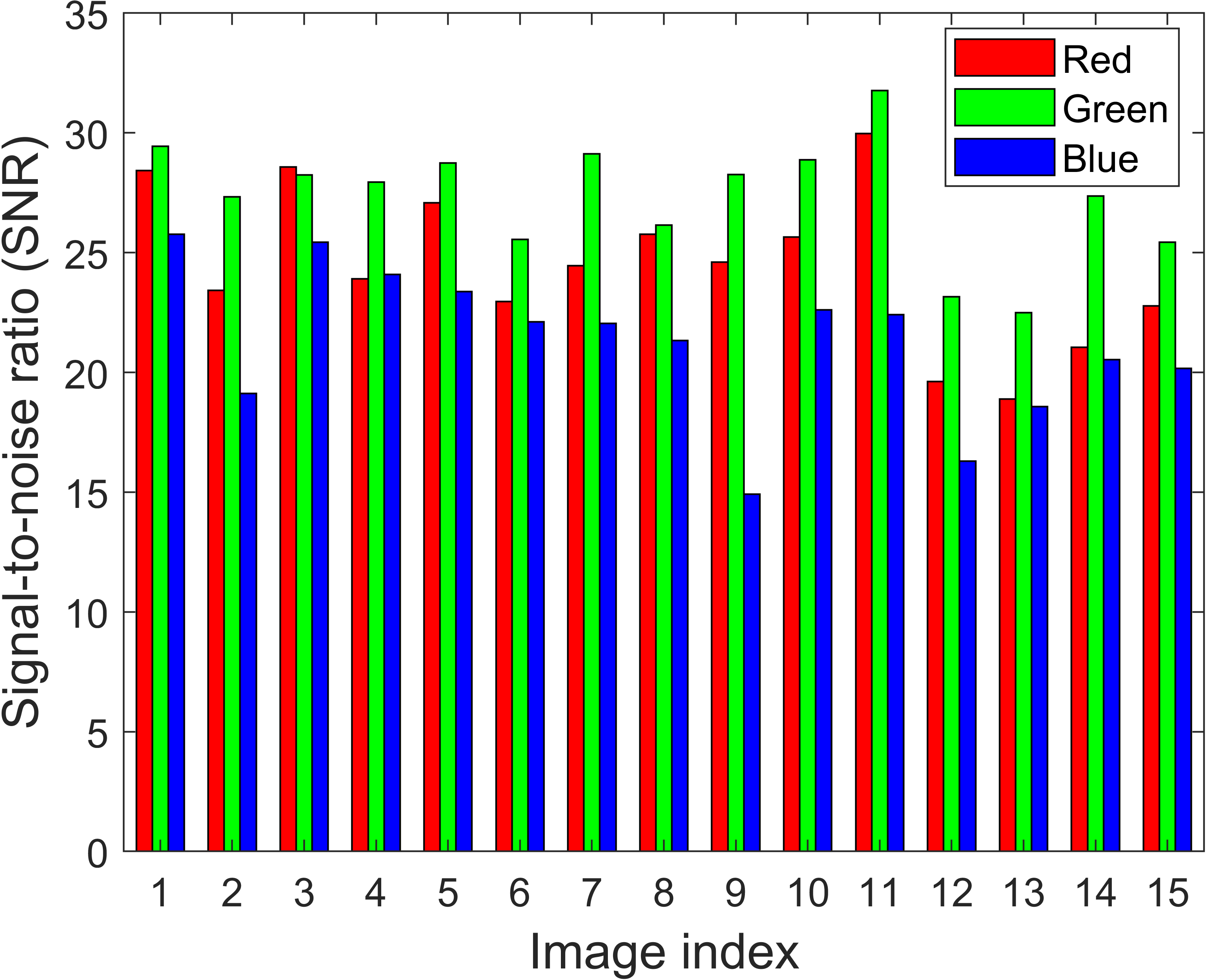
Figure 1: Signal-to-noise ratio (SNR) in RGB channels of 15 real-world images from the CC15 dataset.

To the best of our knowledge, the GCP has not been exploited to guide denoising in the sRGB space. In this paper, we intend to fill this gap and propose GCP-ID, a simple GCP-guided color image denosing method with block circulant representation and t-SVD transform. It is worth mentioning that t-SVD has been adopted by different denoisers [zhang2014novel, kong2019color, shi2021robust], but they all treat each channel as equal.

4 Method

In this section, we present our GCP-ID method in detail. Briefly, GCP-ID consists of three key ingredients: 1) green channel guided patch search, 2) RGGB representation for image patches and 3) nonlocal t-SVD transform. The overall denoising procedure is illustrated in Fig. 2.

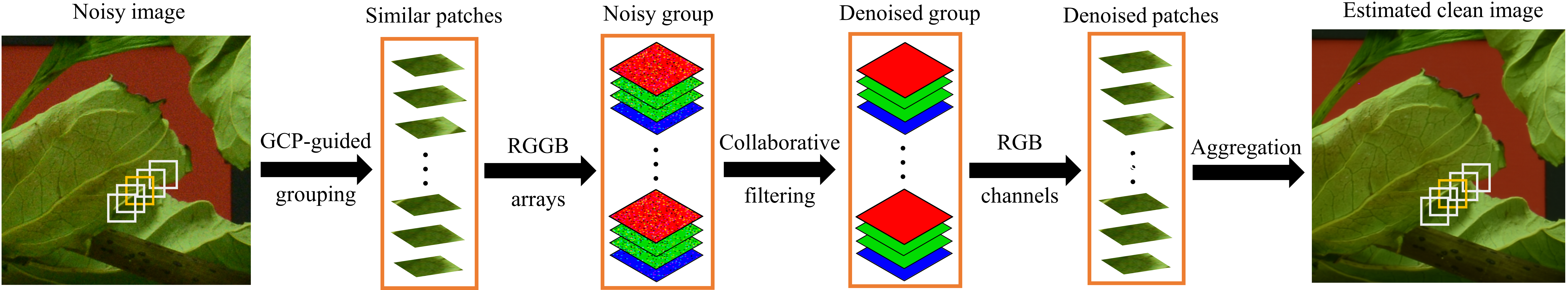
Figure 2: Flowchart of the proposed GCP-ID method for sRGB color image denoising.

4.1 Green Channel Guided Patch Search

Given a color image patch $\mathcal{P}_{ref}\in\mathbb{R}^{N\times N\times 3}$, our goal is to search its $K$ most similar patches in a local window by Euclidean distance. Directly comparing image patches will incur high computational burden. Besides, the presence of complex real-world noise may undermine the patch search process. To efficiently group more closely similar patches, we consider to take advantage of the green channel, which is less noisier and share structural information with red/blue channels. More specifically, we calculate the distance $d$ between image patches via

$$d=\left\{\begin{aligned} &\|\mathcal{P}_{ref}^{G}-\mathcal{P}_{j}^{G}\|,\,\|\mathcal{P}_{ref}^{G}\|\geq\text{max}(\lambda\|\mathcal{P}_{ref}^{R}\|,\lambda\|\mathcal{P}_{ref}^{B}\|)\\ &\|\mathcal{P}_{ref}^{mean}-\mathcal{P}_{j}^{mean}\|_{F},\,\text{otherwise}\end{aligned}\right.$$ (5)

where $\mathcal{P}^{R}$, $\mathcal{P}^{G}$ and $\mathcal{P}^{B}$ represent R, G and B channels, respectively. $\mathcal{P}^{mean}$ is the mean value of RGB channels, which can be regarded as the opponent color space or average pooling operation on RGB channels. $\lambda$ is a threshold parameter that controls the search scheme. In our paper, we empirically set $\lambda=0.8$, and Eq. (5) indicates that the green channel is used for local patch search if its importance is considered larger than certain weights.
To verify the effectiveness of the green channel guided strategy, we compare the patch search successful rate measured by the ratio of patches similar in the underlying clean image. Specifically, for each noisy input of CC15 dataset, we randomly select 1000 reference patches $\mathcal{P}_{ref}\in\mathbb{R}^{8\times 8\times 3}$ and search 60 similar patches for $\mathcal{P}_{ref}$ in a local window of size $20\times 20$. Table 1 reports the average successful rate of different search schemes. The advantage of the green guided strategy will help encourage sparsity in the transform domain, and the correlation among similar image patches can be better captured by learning group-level transform $\mathbf{U}_{group}\in\mathbb{R}^{K\times K}$ via classic methods such as the principal component analysis (PCA) [dabov2009bm3d].

Table 1: Average patch search successful rate of different schemes for noisy images from the CC15 dataset. ‘Green only’: search using only the green channel. ‘Opp’: Opponent color space.

Search scheme	Green only	YCbCr	Opp	Green guided
Successful rate	0.4881	0.4992	0.4938	0.5035

4.2 RGGB Representation

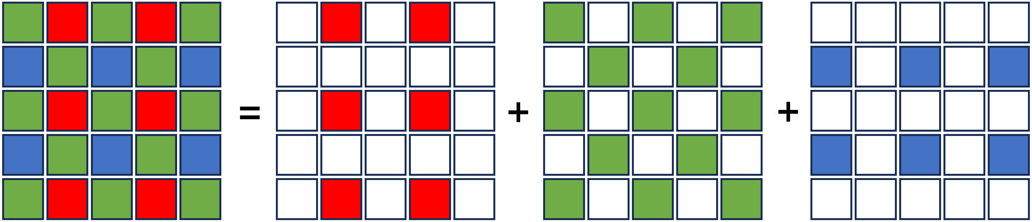
Figure 3: Illustration of the Bayer CFA pattern.

As shown in Fig. 3, the popular Bayer CFA pattern measures the green image on a quincunx grid and the red and blue images on rectangular grids[li2008image]. As a result, the density of the green samples is twice than that of the other two. In practice, the raw Bayer pattern data is not always available, and the interpolation algorithm to reconstruct a full color representation of the image varies according to different camera devices.
To explicitly model the density and importance of the green channel, we reshape each color image patch $\mathcal{P}\in\mathbb{R}^{ps\times ps\times 3}$ into an RGGB array $\hat{\mathcal{P}}\in\mathbb{R}^{ps\times ps\times 4}$ by inserting one extra green channel. Furthermore, to capture the spectral correlation among RGB channels, we use the block circulant matrix $\hat{\mathbf{P}}_{bcirc}\in\mathbb{R}^{4ps\times 4ps}$ to represent the RGGB array. Fig. 4 illustrates the RGGB and block circulant representation (BCR) for an RGB input. The BCR indicates that the density of green channels remains twice than that of red/blue ones in the sRGB space.

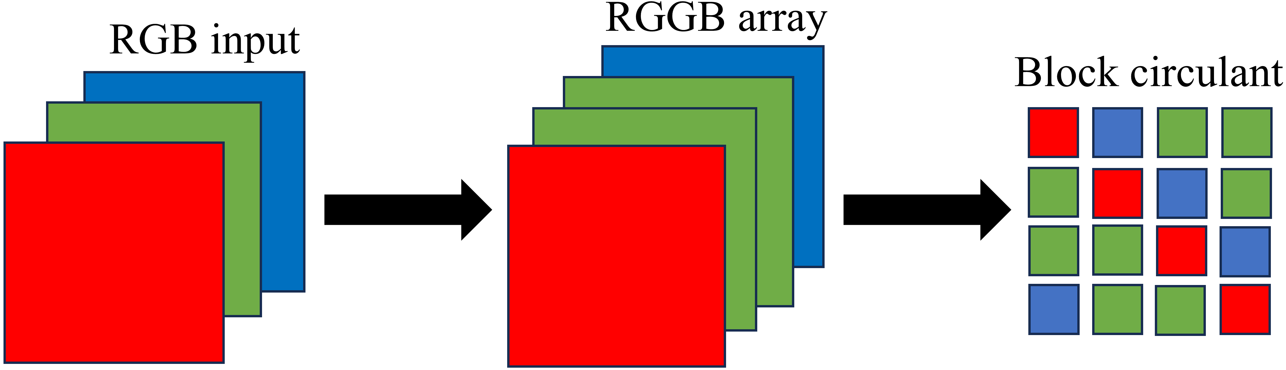
Figure 4: Block circulant representation for an RGB input.

4.3 Nonlocal t-SVD transform

The stacked similar patches often share the same feature space, and a nonlocal generalization of SVD [rajwade2012image] can be explored by learning pairwise projection matrices $\mathbf{U}_{row}\in\mathbb{R}^{4ps\times 4ps}$ and $\mathbf{U}_{col}\in\mathbb{R}^{4ps\times 4ps}$ via

$$\text{min}\sum_{i=1}^{K}\|\hat{\mathbf{P}}_{bcirc_{i}}-\mathbf{U}_{row}\hat{\mathbf{S}}_{bcirc_{i}}\mathbf{U}_{col}^{T}\|^{2}$$ (6)

$$\text{s.t}\quad\mathbf{U}_{row}^{T}\mathbf{U}_{row}=\mathbf{I},\,\mathbf{U}_{col}^{T}\mathbf{U}_{col}=\mathbf{I}$$

where $\hat{\mathbf{S}}_{bcirc_{i}}\in\mathbb{R}^{4ps\times 4ps}$ is the coefficient matrix of $\hat{\mathbf{P}}_{bcirc_{i}}$. From Fig. 4, it is noticed that the RGB channels of $\hat{\mathbf{P}}_{bcirc}$ repeat several times. To efficiently leverage such patch-level redundancy and exploit the spectral correlation among RGB channels, we can take advantage of the nonlocal t-SVD transform to simplify Eq. (6) via

$$\text{min}\sum_{i=1}^{K}\|\hat{\mathcal{P}}_{i}-\mathcal{U}_{row}*\hat{\mathcal{S}}_{i}*\mathcal{U}_{col}^{T}\|_{F}^{2}$$ (7)

$$\text{s.t}\quad\mathcal{U}_{row}^{T}*\mathcal{U}_{row}=\mathcal{I},\,\,\mathcal{U}_{col}^{T}*\mathcal{U}_{col}=\mathcal{I}$$

where $\mathcal{U}_{row}\in\mathbb{R}^{ps\times ps\times 4}$ and $\mathcal{U}_{col}\in\mathbb{R}^{ps\times ps\times 4}$ are a pair of orthogonal tensors, $\hat{\mathcal{S}}_{i}\in\mathbb{R}^{ps\times ps\times 4}$ is the corresponding coefficient tensor of $\hat{\mathcal{P}}_{i}$. Eq. (7) can be solved by slicewise SVD in the Fourier domain after performing the FFT along the third mode of $\hat{\mathcal{P}}$ via

$$\hat{\mathcal{P}}\times_{3}\mathbf{W}_{FFT} =\begin{pmatrix}1&1&1&1\\ 1&-i&-1&i\\ 1&-1&1&-1\\ 1&i&-1&-i\\ \end{pmatrix}\begin{pmatrix}R\\ G\\ G\\ B\\ \end{pmatrix}$$ (8)

$$=\begin{pmatrix}R+2G+B\\ R-G+(B-G)i\\ R-B\\ R-G+(G-B)i\\ \end{pmatrix}$$

Interestingly, from Eq. (8) it can be seen that in the Fourier domain, the first slice models the density of the green channel, the second and fourth slices are complex conjugate that exploit the relationship among RGB channels, and the third slice captures the difference between red and blue channels. Therefore, the RGGB representation also captures the correlation among RGB channels.
Given a group of noisy BCR patches $\hat{\mathcal{G}}_{n}\in\mathbb{R}^{ps\times ps\times 4\times K}$, the overall denoising process of the proposed GCP-ID can be summarized using a one step extension of t-SVD

$$\hat{\mathcal{S}}_{n}=(\mathcal{U}_{row}^{T}*\hat{\mathcal{G}}_{n}*\mathcal{U}_{col})\times_{4}\mathbf{U}_{group}$$ (9)

The hard-thresholding technique [donoho1994ideal] can be applied to shrink the coefficient $\hat{\mathcal{S}}_{n}$ under a certain threshold $\tau$ via

$$\hat{\mathcal{S}}_{truncate}=\left\{\begin{aligned} \hat{\mathcal{S}}_{n},\quad|\hat{\mathcal{S}}_{n}|\geq\tau\\ 0,\quad|\hat{\mathcal{S}}_{n}|<\tau\end{aligned}\right.$$ (10)

The estimated clean group $\hat{\mathcal{G}}_{c}$ can be reconstructed by the inverse transform of Eq. (9) via

$$\hat{\mathcal{G}}_{c}=(\mathcal{U}_{row}*\hat{\mathcal{S}}_{truncate}*\mathcal{U}_{col}^{T})\times_{4}\mathbf{U}_{group}^{T}$$ (11)

Finally, we fetch the RGB channels of $\hat{\mathcal{G}}_{c}$, and each denoised image patch $\mathcal{P}_{c}\in\mathbb{R}^{ps\times ps\times 3}$ is averagely written back to its original location. The implementation of GCP-ID is briefed in Algorithm 1.

Algorithm 1 GCP-ID

Input: Noisy image $\mathcal{Y}\in\mathbb{R}^{M\times N\times 3}$, patch size $ps$, number of similar patches $K$ and search window size $W$.
Output: Estimated clean image $\mathcal{X}\in\mathbb{R}^{M\times N\times 3}$.
Step 1 (Grouping): For each reference patch $\mathcal{P}\in\mathbb{R}^{ps\times ps\times 3}$ of $\mathcal{Y}$, search its $K$ most similar patches within $W$ according to Eq. (5) and stack them in a group $\hat{\mathcal{G}}_{n}\in\mathbb{R}^{ps\times ps\times 4\times K}$ based on RGGB representation.
Step 2 (Collaborative filtering):
    (1) Perform the forward nonlocal t-SVD based on Eq. (9) to obtain the coefficient tensor $\hat{\mathcal{S}}_{n}$, pairwise projection tensors $\mathcal{U}_{row}$, $\mathcal{V}_{row}$ and group-level transform $\mathbf{G}_{group}^{T}$.
    (2) Apply the hard-threshold technique to $\hat{\mathcal{S}}_{n}$ to obtain the truncated coefficient tensor $\hat{\mathcal{S}}_{truncate}$.
    (3) Take the inverse nonlocal t-SVD transform in Eq. (11) to obtain estimated clean group $\hat{\mathcal{G}}_{c}$.
Step 3 (Aggregation): Fetch the RGB channels of $\hat{\mathcal{G}}_{c}$ and averagely write back all denoised image patches.