Causal Discovery under Off-Target Interventions

Abstract

Causal graph discovery is a significant problem with applications across various disciplines. However, with observational data alone, the underlying causal graph can only be recovered up to its Markov equivalence class, and further assumptions or interventions are necessary to narrow down the true graph. This work addresses the causal discovery problem under the setting of stochastic interventions with the natural goal of minimizing the number of interventions performed. We propose the following stochastic intervention model which subsumes existing adaptive noiseless interventions in the literature while capturing scenarios such as fat-hand interventions and CRISPR gene knockouts: any intervention attempt results in an actual intervention on a random subset of vertices, drawn from a distribution dependent on attempted action. Under this model, we study the two fundamental problems in causal discovery of verification and search and provide approximation algorithms with polylogarithmic competitive ratios and provide some preliminary experimental results.

1 Introduction

Learning causal relationships is a fundamental task with applications in many fields, including epidemiology, public health, genomics, economics, and social sciences [Rei56, Hoo90, KWJ⁺04, Woo05, RW06, ES07, CBP16, Tia16, SC17, RHT⁺17, POS⁺18, dCCCM19]. Since the development of Bayesian networks and structural equation modelling, using directed acyclic graphs (DAGs) has been a popular choice to represent causal relationships [SGSH00]. It is well-known that one can recover underlying causal graphs only up to their Markov equivalence class using observational data [VP90, AMP97] and additional assumptions or interventions are necessary if one wishes to uncover the true underlying causal graph. Here, we study causal discovery from interventions with the natural goal of minimizing the number of interventions performed.

Causal discovery using interventional data has been extensively studied with a rich literature of work developing adaptive [SKDV15, GKS⁺19, SMG⁺20, CSB22, CS23b, CS23a] and non-adaptive [EGS05, EGS06, Ebe10, HLV14] strategies. Traditionally, as in most prior works, an experimenter can select a vertex (or a subset of vertices) for intervention and cause the intended intervention with certainty. While simple and elegant, this fails to account for scenarios involving system stochasticity or noise. For example, interventions commonly occur randomly on non-targeted genes in CRISPR gene knockouts [FFK⁺13, WWW⁺15, AWL18] and interventions in psychology [Ero20] are likely to affect variables beyond the target variable. Such interventions are known as off-target or fat-hand interventions, and are prevalent in practical settings [Sch05, EM07, Ebe07, DEMS10, GS17, Ero20]. In this work, we propose and study a stochastic interventional model that aims to model off-target interventions.

1.1 Our off-target intervention model

Suppose $G=(V,E)$ is a causal graph on $|V|=n$ vertices and we have $k\in\mathbb{N}$ possible interventional actions denoted by $A_{1},\dots,A_{k}$. When we perform action $A_{i}$, a subset $S\subseteq V$ is drawn, from the off-target distribution $\mathcal{D}_{i}$ over the power set of vertices $2^{V}$, and intervened upon. See Section 3 for more details and discussion.

Note that our interventional model subsumes the traditional interventional setting when $A_{i}$s are on-target:

$$\mathcal{D}_{i}(S)=\begin{cases}1&\text{if $S=A_{i}$}\\ 0&\text{otherwise}\end{cases}\quad\text{, $\forall S\subseteq V$ and $\forall i\in[k]$}$$

Algorithmic assumptions.

The complete problem is notoriously difficult and one cannot attain guarantees without making assumptions. In this work, we make four key assumptions, each corresponding to a hard problem that is under active exploration. As such, we view our work as initiating the study of a flexible off-target model and establishing the theoretical foundations for the problem of causal discovery under off-target inteventions.

1. The distributions $\mathcal{D}_{1},\ldots,\mathcal{D}_{k}$ are known.

   Knowing the distributions $\mathcal{D}_{i}$ is often a reasonable assumption in practice. For instance, in the case of CRISPR technology, the sequence of a target gene $i$ provides information about which other genes may also be affected. The possible off-target effects are generally well-understood, and one can also build a reasonable estimate of each distribution $\mathcal{D}_{i}$ based on historical data.

   Moreover, when the distributions $\mathcal{D}_{i}$ are unknown, it is straightforward to construct scenarios where any optimal algorithm must, at the very least, partially learn the distributions $\mathcal{D}_{i}$ in order to achieve any non-trivial competitive guarantees; see Appendix B for a discussion on the difficulties in designing algorithms with non-trivial theoretical guarantees when $\mathcal{D}_{i}$’s are unknown.

2. The actual intervened vertices $S$ are observed.

   While we acknowledge that this assumption may be violated in many real-world applications, there have been recent works which infer $S$ from the data [KS21, SWU20]. For instance, [SWU20] argues that, under further assumptions, the actual intervened targets can be recovered by checking which distributions changed after the intervention. We view our work as a preliminary step towards addressing the more general setting where the intervened vertices $S$ is not known to us.

3. We are given access to the essential graph (or equivalently we know the Markov equivalence class) of the true causal graph.

   Under some standard causal assumptions, there are a plethora of algorithms that recover the essential graph from observational data (which is abundant in many applications), such as the PC [SGSH00], FCI [SGSH00] and RFCI algorithms [CMKR12]; see [GZS19, VCB22] for a survey.

4. We are able to determine orientations of edges that are incident to intervened vertices.

   While this is always possible using hard or ideal interventions, this assumption may still hold with weaker forms of interventions (soft, imperfect, shift, etc) under additional conditions.

1.2 Our contributions

We study two fundamental problems in causal graph discovery: verification and search. The former asks the question of checking whether a proposed DAG $G$ from the Markov equivalence class is the true underlying causal DAG $G^{*}$, which serves as a natural lower bound for the latter, which requires us to identify $G^{*}$ from the equivalence class. Our contributions are as follows:

1. We establish a two-way reduction between the off-target verification problem and the well-studied stochastic set covering problem. This equivalence allows us to leverage existing results and techniques in the literature to design our algorithms.

2. We prove that no algorithm can achieve non-trivial competitive approximation guarantees against the off-target verification number, even when all actions have unit weight. This shows the difficulty of the off-target search problem and motivates the need for new benchmarks.

3. Building on our negative result and a recent work [CS23a], we propose algorithms that are competitive against a quantity that captures the performance of any algorithm against the worst-case causal graph within the same Markov equivalence class. Our algorithm runs in polynomial time and is guaranteed to use at most a polylogarithmic number of expected interventions more than the worst-case optimal solution.

One can convert expectation results to high probability ones by paying an extra $\mathcal{O}(\log n)$ factor via standard applications of Markov and Chernoff bounds.

Outline of paper. We begin with preliminary notions and related work in Section 2, then state our main results in Section 3, with details of our verification and search results given in Section 4 and Section 5 respectively. Section 6 shows some experimental results and Section 7 concludes with discussion and future work. For convenience, we will restate our main theorem statements before proving them. Some proofs are deferred to the appendix.

2 Preliminaries and related work

For any set $A$, we use $|A|$ to denote its size and $2^{A}$ to denote its powerset. Let $G=(V,E)$ be a graph on $n$ vertices/nodes. We use $u\sim v$ to denote adjacency, and $u\to v$ or $u\leftarrow v$ to specify directions. For any $v\in V$ in a directed graph, we use $N(v)$ and $\texttt{Pa}(v)$ to denote its neighbors and parents respectively. The skeleton $\mathrm{skel}(G)$ refers to the underlying graph where all edges are made undirected. A v-structure in $G$ refers to three vertices $u,v,w\in V$ such that $u\to v\leftarrow w$ and $u\not\sim w$. For any subset $S\subseteq V$, $G[S]$ denotes the node-induced subgraph of $G$ and $u\in S$ is a source vertex if $u$ has no incoming arcs from any other edges from $S$.

A directed acyclic graph (DAG) is a fully directed graph without directed cycles. We can associate a (not necessarily unique) valid permutation $\sigma:V\to[n]$ to any (partially directed) DAG such that oriented arcs $u\to v$ satisfy $\sigma(u)<\sigma(v)$. For any DAG $G$, we denote its Markov equivalence class (MEC) by $[G]$ and essential graph by $\mathcal{E}(G)$. DAGs in the same MEC $[G]$ have the same skeleton and essential graph $\mathcal{E}(G)$ is a partially directed graph such that an arc $u\to v$ is directed if $u\to v$ in every DAG in MEC $[G]$, and an edge $u\sim v$ is undirected if there exists two DAGs $G_{1},G_{2}\in[G]$ such that $u\to v$ in $G_{1}$ and $v\to u$ in $G_{2}$. It is known that two graphs are Markov equivalent if and only if they have the same skeleton and v-structures [VP90, AMP97]. A DAG is called a moral DAG if it has no v-structures, in which case its essential graph is just its skeleton. An edge $u\to v$ is a covered edge [Chi95] if $\texttt{Pa}(u)=\texttt{Pa}(v)\setminus\{u\}$. We use $C(G)$ to denote the set of covered edges of DAG $G$.

An ideal intervention $S\subseteq V$ is an experiment where all variables $v\in S$ are forcefully set to some value, independent of the underlying causal structure. The effect of interventions is formally captured by Pearl’s do-calculus [Pea09]. Graphically, intervening on $S$ induces a mutilated interventional graph $G_{\bar{S}}$ where all incoming arcs to vertices $v\in S$ are removed [EGS05]. It is known that intervening on $S$ allows us to infer the edge orientation of any edge cut by $S$ and $V\setminus S$ [Ebe07, HEH13, HLV14, SKDV15, KDV17]. An intervention set is a set $\mathcal{I}\subseteq 2^{V}$ of interventions where each intervention corresponds to a subset of variables and an $\mathcal{I}$-essential graph $\mathcal{E}_{\mathcal{I}}(G)$ of $G$ is the essential graph representing the Markov equivalence class of graphs whose interventional graphs for each intervention is Markov equivalent to $G_{\bar{S}}$ for any intervention $S\in\mathcal{I}$. There are several known properties about $\mathcal{I}$-essential graphs [HB12, HB14, CS23b]. For instance, every $\mathcal{I}$-essential graph ($\mathcal{I}$ could be $\emptyset$) is a chain graph with chordal chain components and orientations in one chain component do not affect orientations in other components. So, to fully orient any essential graph $\mathcal{E}(G^{*})$, it is necessary and sufficient to orient every chain component in $\mathcal{E}(G^{*})$. We use $CC(\mathcal{E}(G))$ to denote the set of chain components obtained by ignoring the oriented edges in $\mathcal{E}(G)$, where each $H\in CC(\mathcal{E}(G))$ is a connected undirected subgraph of $G$ and vertices across $H$’s partition $V(G)$. See Fig. 1 for an example.

A verifying set $\mathcal{I}$ for a DAG $G\in[G^{*}]$ is an intervention set that fully orients $G$ from $\mathcal{E}(G^{*})$, possibly with repeated applications of Meek rules (see Appendix C), i.e. $\mathcal{E}_{\mathcal{I}}(G^{*})=G^{*}$. Furthermore, if $\mathcal{I}$ is a verifying set for $G^{*}$, then so is $\mathcal{I}\cup S$ for any additional intervention $S\subseteq V$. While there may be multiple verifying sets in general, we are often interested in finding one with a minimum size/cost. We say that an intervention $S\subseteq V$ cuts an edge $u\sim v\in E$ if $|S\cap\{u,v\}|=1$.

Definition 1 (Minimum size/cost verifying set and verification number/cost).

Let $w$ be a weight function on intervention sets. An intervention set $\mathcal{I}$ is called a verifying set for a DAG $G^{*}$ if $\mathcal{E}_{\mathcal{I}}(G^{*})=G^{*}$. $\mathcal{I}$ is a minimum size (resp. cost) verifying set if $\mathcal{E}_{\mathcal{I}^{\prime}}(G^{*})\neq G^{*}$ for any $|\mathcal{I}^{\prime}|<|\mathcal{I}|$ (resp. for any $w(\mathcal{I}^{\prime})<w(\mathcal{I})$). The minimum verification number $\nu(G)$ and the minimum verification cost $\overline{\nu}(G)$ denote the size/cost of the minimum size/cost verifying set respectively.

There is a rich literature in recovering causal graphs via interventions under various settings such as bounded size interventions, interventions with varying vertex costs, allowing for randomization, modelling as Bayesian approaches, incorporating domain knowledge as constraints, etc. [Hec95, HGC95, CY99, FK00, TK01, Mur01, HG08, MM13, CBP16, HMC06, EGS06, Ebe10, EGS12, HB14, HEH13, HLV14, SKDV15, KDV17, GSKB18, LKDV18, ASY⁺19, GKS⁺19, KSSU19, SMG⁺20, CSB22, TAJ⁺22, TAI⁺23, CS23b, CS23a]. In this work, we are interested in studying off-target interventions where attempting to intervene on vertex $v\in V$ (or a subset of vertices $S\subseteq V$) may result in intervening on other vertices, and possibly not even $v\in V$ itself [Sch05, EM07, Ebe07, DEMS10, GS17, Ero20].

In the context of causal graph discovery via ideal interventions, [CS23b] tells us it suffices to study the verification and search problems on moral DAGs as any oriented arcs in the observational graph can be removed before performing any interventions as the optimality of the solution is unaffected. Below, we review other known results that we later use. For instance, Theorem 3 implies that any topological ordering of the vertices $\sigma$ consistent with the given set of arcs yields a DAG from the same Markov equivalence class.

Theorem 2 (Theorem 9 of [CSB22]).

Any verifying set of a DAG $G$ must cut all the covered edges.

Theorem 3 (Proposition 16 of [HB12], Theorem 7 of [CS23b]).

Given any (interventional) essential graph, any acyclic orientation of the unoriented edges that does not form new v-structures induces a DAG within the same Markov equivalence class.

As mentioned in the introduction, we will relate the problem of verification in our model to the problem of stochastic set cover. Introduced by [GV06], the stochastic set cover is a subproblem in the wider problem domain known as stochastic optimization whereby one wishes to optimize a certain objective under uncertainty (e.g. see [GK11] and references therein).

Problem 4 (Stochastic set cover, with multiplicity).

Consider a set $X$ of $d$ elements and $k$ stochastic sets $S_{1},\ldots,S_{k}$. Each $S_{i}$ is associated with a weight $w_{i}$ and a set-specific distribution $\mathcal{D}_{i}$ where $\mathcal{D}_{i}$ and $\mathcal{D}_{j}$ are independent for $i\neq j$. When $S_{i}$ is picked, a random subset of $X$ is drawn according to $\mathcal{D}_{i}$ and the elements in the subset are said to be covered. The goal is to minimize the weighted set selection cost (sets may be picked multiple times) until all elements in $X$ are covered.

Denoting $\mu_{j}(i)$ as the probability of set $S_{i}$ covering element $j\in X$, [GV06] showed that any policy $\pi$ that succeeds in covering $X$ satisfies the inequality $\sum_{i=1}^{k}\mu_{j}(i)\cdot x_{i}^{\pi}\geq 1$, where $x^{\pi}_{i}$ is the expected number of times $\pi$ picks $S_{i}$. They further showed that minimum expected cost incurred by any adaptive policy $\pi$ for solving 4 is at least the optimal value of (LP):

$$\begin{array}[]{rrlll}\text{minimize}&\sum_{i=1}^{k}w_{i}\cdot x_{i}\\ \text{such that}&\sum_{i=1}^{k}\mu_{j}(i)\cdot x_{i}&\geq&1&,\forall j\in X\\ &x_{i}&\geq&0&,\forall i\in[k]\end{array}$$ (LP)

3 Results

As discussed in the introduction, one of our primary contributions is the definition of a new noisy off-target intervention model. Under this model, we study two fundamental questions: verification and search.

Off-target verification. Under our intervention model, the verification number is defined as follows:

Problem 5 (Off-target verification).

We are given a graph $G=(V,E)$ and $k$ actions $A_{1},\ldots,A_{k}$. For $i\in[k]$, each set $A_{i}$ is associated with a distribution $\mathcal{D}_{i}$, where $\mathcal{D}_{i}$ and $\mathcal{D}_{j}$ are independent for $i\neq j$. When action $A_{i}$ is picked, a random subset of $V$ is drawn according to $\mathcal{D}_{i}$ and the vertices in the subset are intervened upon. The goal is to select as few actions as possible (actions may be picked multiple times) until the interventional essential graph is fully oriented.

From Theorem 2, any verifying set of a DAG $G$ has to cut all covered edges $C(G)$ of $G$. Given actions $A_{1},\ldots,A_{k}$, let $\Pi$ be the space of (possibly randomized) policies that repeatedly pick actions until all covered edges are cut and $x^{\pi}_{i}$ be a random variable that counts the number of times action $A_{i}$ was chosen by policy $\pi\in\Pi$. Then, the off-target verification number and weighted off-target verfication number are given by $\nu(G)=\min_{\pi\in\Pi}\mathbb{E}\left[\sum_{i=1}^{k}x^{\pi}_{i}\right]$ and $\overline{\nu}(G)=\min_{\pi\in\Pi}\mathbb{E}\left[\sum_{i=1}^{k}w_{i}\cdot x^{\pi}_{i}\right]$ respectively, where $w_{i}$ is the cost of choosing action $A_{i}$. When all interventions are on-target, the terms $\nu(G)$ and $\overline{\nu}(G)$ recover existing definitions in the literature.

Our first main technical result is a lower bound on $\overline{\nu}(G^{*})$ and an off-target verification algorithm with a logarithmic competitive ratio. This is made possible by a reduction between the stochastic set cover problem and the off-target verification problem, and then applying known results of [GV06].

Theorem 6.

Stochastic set cover and off-target verification are equivalent. There is a polynomial time adaptive policy which verifies with a cost of $\mathcal{O}(\overline{\nu}(G^{*})\cdot\log n)$ in expectation while obtaining an approximation ratio within $(1-\varepsilon)\cdot\ln n$ is NP-hard for every $\varepsilon>0$.

Theorem 6 essentially tells us that our verification results attain the optimal asymptotic approximation ratio achievable in polynomial time, unless P = NP.

Off-target search. For off-target search, we begin with a rather negative result that no algorithm can provide non-trivial competitive bounds against $\overline{\nu}(G^{*})$, even when all actions have unit cost.

Theorem 7.

For any $n\in\mathbb{N}$, there exists a DAG $G^{*}$ on $n$ nodes and unit-weight actions $A_{1},\ldots,A_{n}$ such that any algorithm pays $\Omega(n\cdot\nu(G^{*}))$ to recover $G^{*}$.

A similar inapproximability result was known in the on-target intervention literature for weighted causal graph discovery [CS23a], in which they proved that no algorithm (even with infinite computational power) can achieve an asymptotically better approximation than $\mathcal{O}(n)$ with respect to the verification cost $\overline{\nu}(G^{*})$ for all ground truth causal graphs on $n$ nodes. The authors of [CS23a] then defined a newer and more nuanced benchmark $\overline{\nu}^{\max}(G^{*})=\max_{G\in[G^{*}]}\overline{\nu}(G)$ which shifts the comparison away from an oracle that knows $G^{*}$ to the best algorithm which knows $[G^{*}]$. Motivated by [CS23a] and Theorem 7, we also compare against $\overline{\nu}^{\max}(G^{*})$ instead of $\overline{\nu}(G^{*})$. To this end, we give an efficient search algorithm that achieves polylogarithmic approximation guarantees against $\overline{\nu}^{\max}(G^{*})$. Our algorithm is based on 1/2-clique graph separators on chordal graphs and heavily relies on the fact that we only need to compete against some causal DAG in the equivalence class. Crucially, $\overline{\nu}^{\max}(G^{*})$ provides us the freedom to force certain unoriented edges to become covered edges judiciously (by competing against some $G^{\prime}\in[G^{*}]$ via Theorem 3) in our search algorithm.

Theorem 8.

Given an essential graph $\mathcal{E}(G^{*})$, there is an algorithm (Algorithm 2) which runs in polynomial time and recovers $G^{*}$ while incurring a cost of $\mathcal{O}(\overline{\nu}^{\max}(G^{*})\cdot\log^{4}n)$ in expectation.

The high-level intuition for the four log factors are as follows (see Section 5 for details): (1) action stochasticity; (2) guessing identities of covered edges; (3) repeated applications of graph separators; (4) additional work to ensure recursion onto smaller subgraphs.

Remark about action distributions and cutting probabilities.

In our problem, we are interested in cutting edges (in particular covered edges; see Theorem 2). For both our verification and search algorithms, all we need are edge cut probabilities $c_{i}(e)\in[0,1]$ of how likely an action $A_{i}$ will cut an edge $e\in E$. Given $\mathcal{D}_{i}$s, one can compute these edge cut probabilities (with time complexities depending on the description of $\mathcal{D}_{i}$s). For example, in the special case where $\mathcal{D}_{i}$s are product distributions over the vertices, i.e. probability of a vertex $v$ being intervened upon is $p_{v}$ and the $p_{v}$s are independent, we have $c_{i}(e=\{u,v\})=\Pr[\text{$A_{i}$ cuts $e$}]=1-p_{u}\cdot p_{v}+(1-p_{u})\cdot(1-p_{v})$. Note that the distributions $\mathcal{D}_{i}$s are independent with respect to the actions, but not necessarily edges: for action indices $i\neq j$ and edges $e\neq e^{\prime}$, $\Pr[A_{i}$ cuts $e]$ is independent of $\Pr[A_{j}$ cuts $e]$ but not necessarily independent of $\Pr[A_{i}$ cuts $e^{\prime}]$.

In the rest of this work, we assume that cutting probabilities, a weaker requirement than $\mathcal{D}_{i}$s, are known. The assumption is weaker because one can derive cutting probabilities from off-target distributions but not vice-versa. For example, consider the case of a single edge $e=\{v_{1},v_{2}\}$ and two possible distinct distributions $\mathcal{D}_{1}$ and $\mathcal{D}_{2}$, where $\mathcal{D}_{i}$ always intervenes on $\{v_{i}\}$: both distributions induce the same cut probability $c(e)$ but we cannot identify $\mathcal{D}_{i}$ simply from $c(e)$. Our algorithms only rely on cut probabilities and does not need the distributions inducing them.

4 Verification

Here we prove our results for the off-target verification problem. In particular, we prove Theorem 6 which shows the equivalence between our off-target verification problem (5) and the stochastic set cover problem (4). The main technical idea behind the reduction follows from Theorem 2, which states that any verifying set must cut all the covered edges of the DAG. The reduction treats covered edges $C(G)$ as the set of elements to cover and an action “covers” a cover edge if the action cuts the covered edge.

Lemma 9.

Every off-target verification instance on causal DAG $G$ with actions $A_{1},\ldots,A_{k}$ and covered edges $C(G)$ corresponds to a stochastic set cover instance on $|C(G)|$ items and stochastic sets $S_{1},\ldots,S_{k}$.

Proof.

To establish a one-to-one correspondence between the two problems, let $X$ be the covered edges $C(G)$ and let each stochastic set $S_{i}$ have exactly the distribution of $A_{i}$. Then, we can solve off-target verification by invoking any algorithm $\mathcal{A}$ for the stochastic set cover problem by choosing action $A_{i}$ whenever $S_{i}$ is being chosen, and informing $\mathcal{A}$ that an element is covered when the corresponding covered edge is cut. ∎

Reduction in the other direction follows by designing a graph where the elements correspond to disjoint covered edges such that sets can be mapped to actions.

Lemma 10.

Every stochastic cover instance with $d$ elements and $k$ stochastic sets $S_{1},\ldots,S_{k}$ corresponds to an off-target verification instance on a causal DAG $G$ with $2d$ vertices, $d$ edges, and $k$ actions $A_{1},\ldots,A_{k}$.

Proof.

For each element $j\in[d]$, we create two vertices $v_{j,1}$ and $v_{j,2}$ and an edge $e_{j}=v_{j,1}\to v_{j,2}$. By construction, $G$ is a collection of $d$ disjoint edges and the set of covered edges is $C(G)=E$. For $i\in[k]$, let us define action $A_{i}$ to be exactly $S_{i}$ on $\{v_{j,1}\}_{j\in[d]}$, i.e. $A_{i}$ assigns the same probability mass as $S_{i}$ to any subset of $\{v_{j,1}\}_{j\in[d]}$ as whatever $S_{i}$ places on element $j$. Thus, the probability of action $A_{i}$ cutting covered edge $e_{j}$ is exactly the probability that $S_{i}$ covers element $j$. Therefore, we can solve the stochastic set cover problem by invoking any algorithm $\mathcal{A}$ for off-target verification problem by choosing set $S_{i}$ whenever $A_{i}$ is being intervened upon, and performing an intervention on $G$ according to the random realization of $S_{i}$. ∎

Theorem 6 follows from our above reductions and by applying Theorems 1 and 2 of [GV06]. To be precise, we invoke CutViaLP (Algorithm 1) with covered edges as the input to provide an efficient approximation algorithm for the off-target verification problem.

See 6

Proof.

The equivalence is via our two-way reductions: Lemma 9 and Lemma 10.

When $\mathcal{D}_{i}$s deterministically map to a single fixed subset of elements, stochastic set cover recovers set cover, which is NP-hard [Kar72]. Thus, stochastic set cover is also NP-hard and so it is NP-hard to exactly solve the off-target verification problem to obtain $\overline{\nu}(G^{*})$. Furthermore, approximating set cover to within a factor of $(1-\varepsilon)\cdot\ln n$ is also NP-hard for any $\varepsilon>0$ [DS14].

To obtain a policy which incurs a cost of at most $\mathcal{O}(\overline{\nu}(G^{*})\cdot\log n)$ in expectation, we can apply Theorems 1 and 2 of [GV06]. To be precise, given a set of $k$ actions $A_{1},\ldots,A_{k}$ and a subset of target edges $T\subseteq E$, consider the following LP adapted from (LP):

$$\begin{array}[]{rrlll}\text{min}&\sum_{i=1}^{k}w_{i}\cdot x_{i}\\ \text{s.t.}&\sum_{i=1}^{k}c_{i}(e)\cdot x_{i}&\geq&1&,\forall e\in T\\ &x_{i}&\geq&0&,\forall i\in[k]\end{array}$$ (VLP)

Theorem 1 of [GV06] tells us that $\overline{\nu}(G^{*})$ is at least the optimal value of (VLP). Meanwhile, Theorem 2 of [GV06] describes a policy which incurs a cost of $\mathcal{O}(\overline{\nu}(G^{*})\cdot\log|T|)\subseteq\mathcal{O}(\overline{\nu}(G^{*})\cdot\log n)$: solve (VLP) with optimal values $x^{*}_{1},\ldots,x^{*}_{k}$, pick $\mathcal{O}(x^{*}_{i}\cdot\log|T|)$ copies of $S_{i}$ in expectation, and repeat this process a constant number of times in expectation to cover all elements (see Algorithm 1). For us, the set $T$ will be instantiated with the set of covered edges $C(G^{*})$ of $G^{*}$. ∎

1:Input: $k$ actions $A_{1},\ldots,A_{k}$, action weights $w_{1},\ldots,w_{k}$, $d$ edges to cut $T\subseteq E$, cutting probabilities $\{c_{i}(e)\}_{i\in[k],e\in T}$.

2:Output: A sequence of attempted interventions such that all edges are cut.

3:Solve (VLP) and let $x^{*}_{1},\ldots,x^{*}_{k}$ be the optimal value and define $y_{i}=9\cdot x_{i}\cdot\ln d$ for all $i\in[k]$.

4:while some edge is still not cut do

5:     for $i\in[k]$ do

6:         Do action $A_{i}$ $\lfloor y_{i}\rfloor$ times deterministically.

7:         With probability $y_{i}-\lfloor y_{i}\rfloor$, do action $A_{i}$.      

Algorithm 1 CutViaLP.

We will later use Algorithm 1 as a subroutine in our off-target search algorithm.

5 Search

We first present a negative result (Theorem 7) which states that one cannot hope to obtain an approximation ratio better than $\Omega(n)$ with respect to the off-target verification number $\overline{\nu}(G^{*})$. Motivated by Theorem 7, we consider the benchmark $\overline{\nu}^{\max}(G^{*})=\max_{G\in[G^{*}]}\overline{\nu}(G)$ defined by [CS23a], against which the authors provided competitive algorithms for causal graph discovery under weighted on-target interventions. In Theorem 8, we provide an efficient approximation search algorithm (Algorithm 2) with polylogarithmic approximation guarantees against $\overline{\nu}^{\max}(G^{*})$.

5.1 Why compare against $\overline{\nu}^{\max}(G^{*})$?

We begin with the negative result that one cannot hope to attain non-trivial approximation to $\overline{\nu}(G^{*})$ even when all actions have unit weights.

See 7

The proof sketch for Theorem 7 is as follows. Consider the star graph on $n$ vertices $v_{1},v_{2},\ldots,v_{n}$ with $v_{n}$ as the center and $v_{1},\ldots,v_{n-1}$ as leaves. Such an essential graph correspond to $n$ possible DAGs, with each vertex as a possible “hidden root”. Suppose there are $n$ unit-weight actions $A_{1},\ldots,A_{n}$ where $\mathcal{D}_{i}$ each deterministically picks the leaf $v_{i}$ (for $1\leq i\leq n-1$) and $\mathcal{D}_{n}$ picks a random leaf uniformly at random. That is, no action will ever intervene on the center vertex $v_{n}$. When any leaf $v_{i}$ is the root node, $\nu(G^{*})=1$ as choosing action $A_{i}$ suffices. However, without knowing the identity of $v_{i}$, one would incur a cost of $\Omega(n)\subseteq\Omega(n\cdot\nu(G^{*}))$.

Meanwhile, observe that $\nu^{\max}(G^{*})=n$ when the center vertex $v_{n}$ is the root node: all edges will be covered edges and we need to cut all of them by intervening on all leaves. Thus, instead of competing against $\nu(G^{*})$, competing against $\nu^{\max}(G^{*})$ would allow for one to design algorithms with more meaningful theoretical guarantees. That is, instead of comparing against an oracle that knows $G^{*}$, we should compare against any algorithm which only knows $\mathcal{E}(G^{*})$. Similar sentiments were also highlighted in recent works [CS23b, CS23a].

Remark (What if a covered edge is never cut?)

From [CSB22], we know that the true causal graph $G^{*}$ will be fully oriented if and only if every covered edge of $G^{*}$ is cut. Therefore, if a cut probability of a certain covered edge is 0, then no algorithm can successfully orient the graph, i.e. $\nu(G^{*})=\infty$. Note that this is not the case for the star graph described above since we are able to cut every edge by intervening on the leaves (via multiple off-target intervention attempts).

5.2 A search algorithm with polylogarithmic approximation to $\overline{\nu}^{\max}(G^{*})$

On a high level, Algorithm 2 repeatedly finds 1/2-clique graph separators (see Theorem 12 below) to break up the chain components so that we can recurse on smaller sized chain components, à la [CSB22, CS23b, CS23a]. See Fig. 1 for an illustration of graphical concepts. However, due to action stochasticities, we encounter new challenges in designing and analyzing a search algorithm for off-target interventions.

Definition 11 ($\alpha$-separator and $\alpha$-clique separator, Definition 19 of [CSB22]).

Let $A,B,C$ be a partition of the vertices $V$ of a graph $G=(V,E)$. We say that $C$ is an $\alpha$-separator if no edge joins a vertex in $A$ with a vertex in $B$ and $|A|,|B|\leq\alpha\cdot|V|$. We call $C$ is an $\alpha$-clique separator if it is an $\alpha$-separator and a clique.

Theorem 12 ([GRE84], instantiated for unweighted graphs).

Let $G=(V,E)$ be a chordal graph with $|V|\geq 2$ and $p$ vertices in its largest clique. There exists a $1/2$-clique-separator $C$ involving at most $p-1$ vertices. The clique $C$ can be computed in $\mathcal{O}(|E|)$ time.

(a) Covered edges $C(G^{*})$ are dashed and $\mathcal{E}(G^{*})=\textrm{skel}(G^{*})$.

(b) $\mathcal{E}(G^{*})$ has a single comp. $H$ with $K_{H}=\{d,g\}$ as a possible 1/2-clique separator.

(c) Connected components after removing $K_{H}$ have size $\leq n/2=4.5$, i.e. “small”.

(d) If $\{g\}$ was intervened upon, the resulting chain component $L_{H}$ is “large”.

Figure 1: A moral DAG $G^{*}$ on $n=9$ nodes illustrating graphical concepts such as $\mathcal{E}(G^{*})$, $\textrm{skel}(G^{*})$, $C(G^{*})$, 1/2-clique separators, and large chain components. The essential graph $\mathcal{E}(G^{*})$ has a single chain component $H$ with $K_{H}$ as one possible 1/2-clique separator of $H$. Suppose we oriented $d\sim g$ through an intervention on $\{g\}$ due to action stochasticity in Fig. 1(d). The resulting chain component $L_{H}$ after intervening on $\{g\}$ is large since $|V(L_{H})|=|\{a,b,c,d,e,f,h,i\}|=8>n/2$. PerformPartitioning (Algorithm 4) breaks $L_{H}$ up by trying to intervene within $L_{H}[V(L_{H})\cap N({\color[rgb]{1,0,0}u_{H}})]$, where $d\equiv{\color[rgb]{1,0,0}u_{H}}$ is the unique vertex from $K_{H}$ within $V({\color[rgb]{1,0,0}K_{H}})\cap V({\color[rgb]{1,0,0}L_{H}})$. There are two chain components $H^{\prime}_{1}$ and $H^{\prime}_{2}$ in the induced subgraph $L_{H}[V(L_{H})\cap N({\color[rgb]{1,0,0}u_{H}})]$. Since $f$ is not a neighbor of $d$, the vertex $f$ is not part of $H^{\prime}_{2}$. If we pick 1/2-clique separators $Z^{\prime}_{1}=\{b,c\}$ and $Z^{\prime}_{2}=\{e,h\}$ for $H^{\prime}_{1}$ and $H^{\prime}_{2}$, then $c\equiv{\color[rgb]{.75,0,.25}z^{\prime}_{1}}$ and $e\equiv{\color[rgb]{.75,0,.25}z^{\prime}_{2}}$ are the sources of $Z^{\prime}_{1}$ and $Z^{\prime}_{2}$ respectively.

1:Input: Essential graph $\mathcal{E}(G^{*})$ of a moral DAG $G^{*}$, $k$ actions $A_{1},\ldots,A_{k}$, action weights $w_{1},\ldots,w_{k}$, cutting probabilities $\{c_{i}(e)\}_{i\in[k],e\in E}$.

2:Output: A complete orientation of $G^{*}$.

3:while there are still unoriented edges do

4:     $K\leftarrow\emptyset$ $\triangleright$ Collection of 1/2-clique separators.

5:     for each chain comp. $H$ of size $|V(H)|\geq 2$ do

6:         Find 1/2-clique separator $K_{H}$ of $H$.

7:         Add $K_{H}$ to $K$ and store the size of $|V(H)|$.      

8:     Run PerformPartitioning on $K$.

Algorithm 2 OffTargetSearch.

To appreciate of some of the new challenges, consider the simple case where the input essential graph $\mathcal{E}(G^{*})$ is a clique on $n$ vertices. If $G^{*}$ orients $v_{1}\to\ldots\to v_{n}$, then the covered edges are $C(G^{*})=\{v_{1}\to v_{2},\ldots,v_{n-1}\to v_{n}\}$. By Theorem 2, interventions need to cut all edges in $C(G^{*})$ to fully orient $\mathcal{E}(G^{*})$. However, we do not actually know the true edge orientations of $G^{*}$ (and hence $C(G^{*})$). To orient $\mathcal{E}(G^{*})$, [CSB22, CS23b] simply intervene on all vertices while [CS23a] intervenes on all vertices except the costliest vertex. In either case, these prior works are guaranteed to fully orient $\mathcal{E}(G^{*})$ regardless of the underlying orientation of $G^{*}$ while paying $\mathcal{O}(\overline{\nu}^{\max}(G^{*}))$. Unfortunately, with off-target interventions, such strategies do not work as it may be too costly to attempt to intervene on each vertex one at at time.

While an 1/2-clique separator approach typically ensures that search completes in $\mathcal{O}(\log n)$ iterations if we can repeatedly identify separators and recurse on smaller subgraphs, action stochasticities may prevent us from orienting all incident edges to the separators. We overcome this via the subroutine PerformPartitioning (Algorithm 4) described later.

Lemma 13.

If resulting components in $H$ always have size at most $|V(H)|/2$ after invoking PerformPartitioning, then OffTargetSearch terminates in $\mathcal{O}(\log n)$ iterations and outputs $G^{*}$.

To understand PerformPartitioning, we first need to describe the subroutine OrientInternalCliqueEdges (Algorithm 3) used to orient internal edges within any collection of disjoint cliques.

1:Input: Target edges $T\subseteq E$ of disjoint cliques.

2:Output: A complete orientation of all edges in $T$.

3:while there are still unoriented edges in $T$ do

4:     Pick an arbitrary topological ordering $\sigma$ that is consistent with all revealed arc orientations.

5:     Run CutViaLP on the covered edges w.r.t. $\sigma$.

Algorithm 3 OrientInternalCliqueEdges.

Lemma 14.

OrientInternalCliqueEdges incurs a cost of $\mathcal{O}(\overline{\nu}^{\max}(G^{*})\cdot\log^{2}n)$ in expectation.

We can obtain competitive ratios against $\overline{\nu}^{\max}(G^{*})$ as we can freely orient unoriented edges in an acyclic fashion to obtain a DAG within the equivalence class (Theorem 3). One logarithmic factor is due to stochasticity while invoking CutViaLP (Algorithm 1); in a similar spirit as the coupon collector problem. Meanwhile, the other logarithmic factor is because we do not know the identities of the covered edges within the cliques. In more detail: after a call to CutViaLP on an arbitrary ordering $\sigma$, we are guaranteed that no two adjacent vertices (with respect to $\sigma$) will be in the same chain component (Theorem 18), so the size of each clique is at least halved and logarithmic rounds suffice.

1:Input: A collection of 1/2-clique separators $K=\{K_{H}\}_{H\in CC(\mathcal{E}_{\mathcal{I}}(G^{*}))}$, for some $\mathcal{E}_{\mathcal{I}}(G^{*})$.

2:Output: An interventional essential graph where sizes of chain components in $H$ are $\leq|H|/2$.

3:Run OrientInternalCliqueEdges on $E(K)$ to get interventional essential graph $\mathcal{E}_{\mathcal{I}^{\prime}}(G^{*})$.

4:Let $L=\{L_{H}\in H:|V(L_{H})|>|V(H)|/2\}$ be the large chain components with unique vertex $u_{H}\in V(K_{H})\cap V(L_{H})$ for each $L_{H}\in L$. $\triangleright$ Lemma 15

5:while $\exists L_{H}\in L$ such that $|V(L_{H})|\geq 2$ do

6:     Find 1/2-clique separator $Z_{H^{\prime}}$ of $H^{\prime}$ for each $L_{H}\in H$ and $H^{\prime}\in CC(L_{H}[V(L_{H})\cap N(u_{H})])$.

7:     Define a consistent ordering $\sigma$ s.t. for all $L_{H}\in L$ and $H^{\prime}\in CC(L_{H}[V(L_{H})\cap N(u_{H})])$, we have

8:     $\sigma(u_{H})<\sigma(z)<\sigma(y)$ for all $z\in V(Z_{H^{\prime}})$, and for all $y\in V(H^{\prime})\setminus V(Z_{H^{\prime}})$.

9:     Run OrientInternalCliqueEdges on the covered edges w.r.t. $\sigma$. For each $H^{\prime}$, let $z_{H^{\prime}}$ be the source

10:     vertex of $Z_{H^{\prime}}$ which we can identify after orienting internal edges.

11:     Define a consistent ordering $\sigma^{\prime}$ s.t. for all $L_{H}\in L$ and $H^{\prime}\in CC(L_{H}[V(L_{H})\cap N(u_{H})])$, we have

12:     $\sigma^{\prime}(u_{H})<\sigma^{\prime}(z_{H^{\prime}})<\sigma^{\prime}(y)$ for all $y\in V(L_{H})\setminus\{u_{H},z_{H^{\prime}}\}$.

13:     Run CutViaLP on the covered edges w.r.t. $\sigma^{\prime}$. $\triangleright$ $u_{H}\sim z_{H^{\prime}}$ is a covered edge

14:     Restrict $L_{H}$s to the component with $u_{H}$s.

Algorithm 4 PerformPartitioning.

Given 1/2-clique separators for chain components of an essential graph $\mathcal{E}_{\mathcal{I}}(G^{*})$, PerformPartitioning first invokes OrientInternalCliqueEdges to orient the edges internal to the separators, yielding a new interventional essential graph $\mathcal{E}_{\mathcal{I}^{\prime}}(G^{*})$. For an arbitrary chain component $H$, there may still be unoriented edges incident to separator vertices as some vertices may not be intervened by OrientInternalCliqueEdges. A resulting chain component $L_{H}\in CC(\mathcal{E}_{\mathcal{I}^{\prime}}(G^{*}))[H]$ is considered “large” if its size is strictly larger than $|V(H)|/2$; if it exists, there can be at most one of them for each $H$.

Lemma 15.

Consider the interventional essential graph $\mathcal{E}_{\mathcal{I}^{\prime}}(G^{*})$ at Line 1 of Algorithm 4 and an arbitrary chain component $H\in CC(\mathcal{E}_{\mathcal{I}}(G^{*}))$. If $\mathcal{E}_{\mathcal{I}^{\prime}}(G^{*})[H]$ has a large chain component $L_{H}$ of size $|V(L_{H})|>|V(H)|/2$, then $|V(L_{H})\cap V(K_{H})|=1$ for any 1/2-clique separator $K_{H}$ of $H$.

Fix a large component $L_{H}$. By Lemma 15, $L_{H}$ contains exactly one vertex from $K_{H}$, say $u_{H}$. By the property of 1/2-clique separators, $L_{H}[V(L_{H})\setminus\{u_{H}\}]$ consists of components of size at most $|V(H)|/2$. That is, orienting all edges incident to $u_{H}$ suffices to break up $L_{H}$ into small components. However, this may be costly. Instead, we use separators while invoking OrientInternalCliqueEdges and CutViaLP.

Lemma 16.

Fix any chain component $H$ and consider any chain component $H^{\prime}\in CC(L_{H}[V(L_{H})\cap N(u_{H})])$. PerformPartitioning cuts $u_{H}\sim z_{H^{\prime}}$ either in Line 6 or 8. If $u_{H}$ is still connected to some chain component $C\subseteq H^{\prime}$ after Line 8, then $|V(C)|\leq|V(H^{\prime})|/2$.

Note that, within the while-loop, it may be the case that $H^{\prime}$ is a singleton $\{z_{H^{\prime}}\}$ (e.g. when $L_{H}$ is a large star with $u_{H}$ at the center). In this case, the edge $u_{H}\sim z_{H^{\prime}}$ will be cut on Line 8.

Throughout, to compete against $\overline{\nu}^{\max}(G^{*})$, we only need to compete against some causal DAG in the equivalence class and apply Theorem 3 in our analysis suitably. As PerformPartitioning uses $\mathcal{O}(\log n)$ iterations to remove large chain components, and each iteration of the while loop invokes OrientInternalCliqueEdges and CutViaLP once, we have:

Lemma 17.

PerformPartitioning incurs a cost of at most $\mathcal{O}(\overline{\nu}^{\max}(G^{*})\cdot\log^{3}n)$ per invocation, and chain components in $H$ always have size at most $|V(H)|/2$ after invoking PerformPartitioning.

Our search result (Theorem 8) immediately follows by combining Lemma 13 and Lemma 17.

6 Experiments

While our main contributions are theoretical, we also implemented our algorithms and performed some experiments; see Appendix E for more details and plots.

Each experimental instance is defined on some hidden ground truth DAG $G^{*}$ along with the off-target distributions $\mathcal{D}_{i}$s. A search algorithm aims to recover $G^{*}$ with as few interventions as possible while only given the partially oriented essential graph of $G^{*}$ and the cutting probabilities derived from $\mathcal{D}_{i}$s as input.

Algorithms. As our off-target intervention setting has not been studied before from an algorithmic perspective, there is no suitable prior work to compare against. We adapted existing state-of-the-art adaptive on-target intervention algorithms in a generic way: we solve (VLP), interpret the optimal vector $X$ as a probability distribution $p$ over the actions, then repeatedly sample from $p$ until the desired on-target intervention is completed before picking the next one. We also show the optimal value of (VLP), along with performance of the naive Random and a One-shot baselines.

Graph instances. We tested on synthetic GNP_TREE graphs [CS23b] of various sizes, and on some real-world graphs from bnlearn [Scu10]. We associate a unit-cost action $A_{v}$ to each vertex $v\in V$ of the input graph.

Interventional distributions. We designed 3 types of off-target interventions when taking action $A_{v}$.
(1) $r$-hop: Sample a uniform random vertex from $r$-hop neighborhood of $v$, including $v$ itself.
(2) Decaying: Sample a random vertex from $V$, with probability decreasing as we move from $v$.
(3) Fat finger: Intervene on $v$, and also possibly on some neighbors of $v$ at the same time.

Qualitative conclusions. There is no prior baseline as we are the first to study off-target interventions from an algorithmic standpoint. Although empirical gains are not significant over some algorithms we adapted from other settings, we have theoretical guarantees for off-target interventions while they don’t. Random and One-shot fare poorly while our method is visibly better or at least competitive with the adapted on-target methods. Regardless, note that our algorithm has provable guarantees even for non-uniform action costs and it is designed to handle worst-case off-target instances.

7 Conclusion and discussion

We studied causal graph discovery under off-target interventions. Under our model, verification is equivalent to the well-studied problem of stochastic set cover and so we inherit existing approximation results from that literature. For search, we argued that no algorithm can provide meaningful approximations to $\overline{\nu}(G^{*})$, and we provided an algorithm with polyalgorithmic approximation guarantees against $\overline{\nu}^{\max}(G^{*})$.

Open directions. We assumed known cutting probabilities $c_{i}(e)$ and intervened sets $S$. More generally, our theoretical guarantees relied on some standard causal inference assumptions in the literature and we view our work as laying the theoretical foundations for studying off-target interventions. For a wider applicability, it is of great interest to validate/weaken/remove these assumptions. In particular, extending our results into the finite sample regime would be very exciting.

Acknowledgements

This research/project is supported by the National Research Foundation, Singapore under its AI Singapore Programme (AISG Award No: AISG-PhD/2021-08-013). KS and CU were partially supported by the Eric and Wendy Schmidt Center at the Broad Institute, NCCIH/NIH (1DP2AT012345), ONR (N00014-22-1-2116), the MIT-IBM Watson AI Lab, and a Simons Investigator Award (to CU). We would like to thank the reviewers for valuable feedback and discussions.

Appendix A Augmenting the preliminaries

“Cutting an edge” behaves differently from “intervening on one of the endpoints of that edge”. Consider a triangle $u\sim v\sim w\sim u$. The non-atomic intervention $\{v,w\}$ cuts the edge $u\sim v$ but not the edge $v\sim w$ because $|\{u,v\}\cap\{v,w\}|=1$ while $|\{v,w\}\cap\{v,w\}|=2\neq 1$. So, one would expect the edge $\{v,w\}$ to remain unoriented unless Meek rules apply. For example, see Fig. 2:

Example 1

If the ground truth DAG was $u\to v\leftarrow w\leftarrow u$, then intervening on $\{v,w\}$ will only orient $u\to v$ and $u\to w$ while $w\to v$ remains unoriented.

Example 2

If the ground truth DAG was $u\leftarrow v\to w\leftarrow u$, then intervening on $\{v,w\}$ orients $u\leftarrow v$ and $w\leftarrow u$, and then Meek rule R2 orients $v\to w$ via $v\to u\to w\sim v$.

Figure 2: Illustrating the difference between cutting an edge and intervening on one of the endpoints of that edge on the moral graph $u\sim v\sim w\sim u$. In both examples, the non-atomic intervention $\{v,w\}$ cuts the edges $u\sim v$ and $u\sim w$ but not $v\sim w$. In the first case, $v\sim w$ remains unoriented. In the second case, $v\sim w$ is oriented due to Meek rules.

The following known results will be useful for our proofs later.

Theorem 18 (Theorem 7 of [CS23b]).

If $G$ is a moral DAG and an arc $u\to v$ is oriented in an (interventional) essential graph of $G$, then $u$ and $v$ belong to different chain components.

Recall the problem of stochastic set cover with multiplicity, defined in Section 2: See 4

Theorem 19 states the known results of [GV06] pertaining to 4.

Theorem 19 (Theorems 1 and 2 of [GV06]).

Any adaptive policy $\pi$ for solving 4 is at least the optimal value of (LP). Meanwhile, there is a polynomial time non-adaptive policy for solving 4 such that it incurs a cost of at most $12\ln d$ times the cost incurred by an optimal adaptive policy: solve (VLP) with optimal values $x^{*}_{1},\ldots,x^{*}_{k}$, pick $\mathcal{O}(x^{*}_{i}\cdot\log|T|)$ copies of $S_{i}$ in expectation, and repeat this process a constant number of times in expectation to cover all elements (see Algorithm 1).

Note that obtaining an approximation ratio within $(1-\varepsilon)\cdot\ln n$ is NP-hard for any $\varepsilon>0$, so multiplicative overhead of $12\ln d$ is asymptotically optimal.

Appendix B Unknown off-target distributions $\mathcal{D}_{i}$s

Here, we discuss difficulties in designing algorithms with non-trivial theoretical guarantees when $\mathcal{D}_{i}$s are unknown. These difficulties persist even if we know the covered edges.

Consider the following toy example where the essential graph is a tree. That is, the underlying causal DAG is some rooted tree with an unknown root node $v^{*}$ and the covered edges are the edges incident to $v^{*}$. So, to fully orient the graph, we need to cut all the edges incident to $v^{*}$. Regardless of the number of actions $k$, there could be only one action $A_{i^{*}}$ with corresponding distribution $\mathcal{D}_{i^{*}}$ with non-zero probability of cutting the covered edges; all other $A_{i}$s (for $i\not=i^{*}$) will never cut any covered edge. Clearly, the optimal algorithm should only repeatedly take action $A_{i^{*}}$ until all the covered edges are cut. Meanwhile, if we do not know the $\mathcal{D}_{i}$s, then there is no hope for designing algorithms with non-trivial theoretical guarantees, even against $\overline{\nu}^{\max}(G^{*})$: an algorithm that knows the $\mathcal{D}_{i}$s only picks a single action $A_{i^{*}}$ while any other algorithm would need to try all actions.

Note that in our lower bound result and construction (Theorem 7), the $\mathcal{D}_{i}$s are known. Yet, despite this, no algorithm can have a competitive ratio better than $\Omega(n)$ against $\overline{\nu}(G^{*})$; but competitiveness against $\overline{\nu}^{\max}(G^{*})$ is possible.

Appendix C Meek rules

Meek rules are a set of 4 edge orientation rules that are sound and complete with respect to any given set of arcs that has a consistent DAG extension [Mee95]. Given any edge orientation information, one can always repeatedly apply Meek rules till a fixed point to maximize the number of oriented arcs.

Definition 20 (Consistent extension).

A set of arcs is said to have a consistent DAG extension $\pi$ for a graph $G$ if there exists a permutation on the vertices such that (i) every edge $\{u,v\}$ in $G$ is oriented $u\to v$ whenever $\pi(u)<\pi(v)$, (ii) there is no directed cycle, (iii) all the given arcs are present.

Definition 21 (The four Meek rules [Mee95], see Fig. 3 for an illustration).

R1

Edge $\{a,b\}\in E\setminus A$ is oriented as $a\to b$ if $\exists$ $c\in V$ such that $c\to a$ and $c\not\sim b$.

R2

Edge $\{a,b\}\in E\setminus A$ is oriented as $a\to b$ if $\exists$ $c\in V$ such that $a\to c\to b$.

R3

Edge $\{a,b\}\in E\setminus A$ is oriented as $a\to b$ if $\exists$ $c,d\in V$ such that $d\sim a\sim c$, $d\to b\leftarrow c$, and $c\not\sim d$.

R4

Edge $\{a,b\}\in E\setminus A$ is oriented as $a\to b$ if $\exists$ $c,d\in V$ such that $d\sim a\sim c$, $d\to c\to b$, and $b\not\sim d$.

Figure 3: An illustration of the four Meek rules

There exists an algorithm (Algorithm 2 of [WBL21]) that runs in $\mathcal{O}(d\cdot|E|)$ time and computes the closure under Meek rules, where $d$ is the degeneracy of the graph skeleton.

Appendix D Deferred proofs

It would be helpful to keep the definition of

$$\overline{\nu}^{\max}(G^{*})=\max_{G\in[G^{*}]}\overline{\nu}(G)$$

and Theorem 6 (which we restate below for convenience) in mind for our proofs below.

See 6

The following lemma bounds the cost incurred by CutViaLP to $\overline{\nu}^{\max}(G^{*})$ using Theorem 19 when we invoke CutViaLP on a subset of covered edges of some DAG $G^{\prime}\in[G^{*}]$.

Lemma 22.

If we invoke CutViaLP on a subset of covered edges $T$ of some DAG $G^{\prime}\in[G^{*}]$, then CutViaLP incurs a cost of $\mathcal{O}(\overline{\nu}(G^{\prime})\cdot\log|T|)\subseteq\mathcal{O}(\overline{\nu}^{\max}(G^{*})\cdot\log n)$ in expectation.

Proof.

As $T$ is a subset of covered edges $C(G^{\prime})$ of some DAG $G^{\prime}\in[G^{*}]$, Theorem 19 tells us that CutViaLP incurs a cost of $\mathcal{O}(\overline{\nu}(G^{\prime})\cdot\log|T|)$ in expectation. The claim follows as $|T|\leq n$ and $\overline{\nu}^{\max}(G^{*})=\max_{G\in[G^{*}]}\overline{\nu}(G)$. ∎

See 7

Proof.

Consider the star graph on $n$ vertices $v_{1},v_{2},\ldots,v_{n}$ with $v_{n}$ as the center and $v_{1},\ldots,v_{n-1}$ as leaves (Fig. 4). Such an essential graph is a tree and corresponds to $n$ possible DAGs, with one of the vertices as a “hidden root” node. Suppose there are $n$ unit-weight actions $A_{1},\ldots,A_{n}$ where $\mathcal{D}_{i}$ each deterministically picks the leaf $v_{i}$ (for $1\leq i\leq n-1$) and $\mathcal{D}_{n}$ picks a random leaf uniformly at random. That is, no action will ever intervene on the center vertex $v_{n}$.

Figure 4: A star graph with $v_{n}$ as the center.

Orienting $G^{*}$ from the essential graph is exactly finding the hidden root leaf node, which corresponds to the problem of searching for a specific number in an unsorted array with $n-1$ numbers. It is well-known that any algorithm (even randomized ones) incurs $\Omega(n)$ array probes for the problem of searching in an unsorted array (e.g. see Theorem 15.1 of [Sha13]). Since our setting restricts the set of actions (pick each index deterministically or choosing a random index uniformly at random) on the same problem, it also has a lower bound of $\Omega(n)$. Note that the lower bound of $\Omega(n)$ holds both in the worst-case and in expectation.

Meanwhile, recall that the actions $A_{i}$ are deterministically picks the leaf $v_{i}$, for $1\leq i\leq n-1$. So, $\nu(G^{*})=1$ by taking action $A_{i^{*}}$ to intervene on $v_{i^{*}}$, where $i^{*}\in[n-1]$ is the index of the hidden root leaf node.

Therefore, any algorithm pays $\Omega(n\cdot\nu(G^{*}))$ to fully recover $G^{*}$ (both in the worst case and in expectation). ∎

See 13

Proof.

When a chain component has size 1, it means that incident edges to that singleton vertex are oriented. Since the size of the chain components decreases by a factor of two in each phase, $\mathcal{O}(\log n)$ iterations suffices. ∎

See 14

Proof.

We first argue that OrientInternalCliqueEdges runs for $\mathcal{O}(\log|T|)\subseteq\mathcal{O}(\log n)$ while-loop iterations then argue that it incurs a cost of $\mathcal{O}(\overline{\nu}^{\max}(G^{*})\cdot\log n)$ in expectation per iteration.

Upper bounding the number of iterations

Consider an arbitrary while-loop iteration. Suppose the largest connected component (induced by edges of $T$) is of size $k$, where $1\leq k\leq\sqrt{|T|}$. When $k=1$, all internal clique edges are oriented. Suppose the vertices in this component are $v_{1},\ldots,v_{k}$.

Fix an arbitrary ordering $\sigma$. Without loss of generality, by relabelling, suppose that $\sigma(v_{1})<\ldots<\sigma(v_{k})$. Under this ordering, we see that $v_{1}\sim v_{2},\ldots,v_{k-1}\sim v_{k}$ are covered edges which will be cut when we invoke CutViaLP. By Theorem 18, we are guaranteed that no two adjacent vertices (with respect to $\sigma$) will be in the same chain components after invoking CutViaLP. To be precise, for $1\leq i\leq k-1$, there exists an intervention where exactly one of $v_{i}$ and $v_{i+1}$ will be intervened upon, so the edge $v_{i}\sim v_{i+1}$ becomes oriented, thus $v_{i}$ and $v_{i+1}$ be in different chain components.

Note that any chain component of size strictly larger than $\lceil k/2\rceil+1$ within this size $k$ chain component includes two adjacent vertices (with respect to $\sigma$ index ordering). This cannot happen by the above argument, so we can conclude that the size of the largest connected component drops by a constant factor in each while-loop iteration, and thus OrientInternalCliqueEdges runs for $\mathcal{O}(\log|T|)$ while-loop iterations.

Crucially, the resulting chain components are again a collection of disjoint cliques, so the above argument can be repeated recursively. It is again a collection of disjoint cliques because edges exist between any pair of vertices (since $T$ was originally a set of edges that induce a collection of disjoint cliques) and oriented edges cannot have endpoints in the same chain component due to Theorem 18.

Upper bounding the cost per iteration

Fix an arbitrary while-loop iteration. By Theorem 3, the set of covered edges $T^{\prime}$ induced by the arbitrarily chosen $\sigma$ is a subset of covered edges of some $G^{\prime}\in[G^{*}]$. By Lemma 22, CutViaLP incurs a cost of $\mathcal{O}(\overline{\nu}^{\max}(G^{*})\cdot\log n)$ in expectation. ∎

See 15

Proof.

We will first argue that $L_{H}$ contains at least one vertex from $K_{H}$ and then argue that $L_{H}$ contains at most one vertex from $K_{H}$.

Contains at least one

Since $K_{H}$ was a 1/2-clique separator of $H$, if $L_{H}$ did not contain any vertices from $K_{H}$, then we must have $|L_{H}|\leq|V(H)|/2$. So, $L_{H}$ includes at least one vertex from $K_{H}$.

Contains at most one

Suppose, for a contradiction, that $L_{H}$ includes more than one vertex from the clique $K_{H}$, say $u$ and $v$. After invoking OrientInternalCliqueEdges, the edge $u\sim v$ should be oriented. So, according Theorem 18, $u$ and $v$ should not be in the same chain component. This is a contradiction to the assumption that the chain component $L_{H}$ includes both $u$ and $v$. ∎

See 16

Proof.

We first argue that PerformPartitioning will cut $u_{H}\sim z_{H^{\prime}}$ either in Line 6 or 8. Suppose Line 6 did not cut $u_{H}\sim z_{H^{\prime}}$. Then, under $\sigma^{\prime}$, the edge $u_{H}\sim z_{H^{\prime}}$ will be an unoriented covered edge and will be cut in Line 8.

Now suppose $u_{H}$ is still connected to some chain component $C\subseteq H^{\prime}$ after Line 8. Upon cutting $u_{H}\sim z_{H^{\prime}}$, the edge becomes oriented and so the vertices $u_{H}$ and $z_{H^{\prime}}$ will belong in different chain components thereafter (Theorem 18), so $z_{H^{\prime}}\not\in V(C)$. After Line 6, OrientInternalCliqueEdges ensures that internal edges of $Z_{H^{\prime}}$ are oriented. Now, since $V(C)\setminus\{u_{H}\}\subseteq V(H^{\prime})$ and $Z_{H^{\prime}}$ was a 1/2-clique separator for $H^{\prime}$, we see that $|V(C)|\leq|V(H^{\prime})|/2$. ∎

Note that the number of chain components within $L_{H}$ may increase during the while-loop but we will only concern ourselves with the chain component that is still connected to $u_{H}$. In other words, $L_{H}$ may break into multiple chain components, but at most one will contain $u_{H}$. See Fig. 5 for an example illustration.

(a) Covered edges $C(G^{*})$ are dashed and $\mathcal{E}(G^{*})=\textrm{skel}(G^{*})$.

(b) If $\{g\}$ was intervened upon, the resulting chain component $L_{H}$ is “large”.

(c) Intervening on $\{a,c\}$ orients the red edges, then Meek rules orient the blue edges.

(d) The resulting chain component after removing oriented edges.

Figure 5: Recall the moral DAG $G^{*}$ on $n=9$ nodes given in Fig. 1. Suppose we oriented $d\sim g$ through an intervention on $\{g\}$ due to action stochasticity in Fig. 5(b). The resulting chain component $L_{H}$ after intervening on $\{g\}$ is large since $|V(L_{H})|=|\{a,b,c,d,e,f,h,i\}|=8>n/2$. PerformPartitioning (Algorithm 4) breaks $L_{H}$ up by trying to intervene within $L_{H}[V(L_{H})\cap N({\color[rgb]{1,0,0}u_{H}})]$, where $d\equiv{\color[rgb]{1,0,0}u_{H}}$ is the unique vertex from $K_{H}$ within $V({\color[rgb]{1,0,0}K_{H}})\cap V({\color[rgb]{1,0,0}L_{H}})$. There are two chain components $H^{\prime}_{1}$ and $H^{\prime}_{2}$ in the induced subgraph $L_{H}[V(L_{H})\cap N({\color[rgb]{1,0,0}u_{H}})]$. Let us focus our remaining discussion on $H^{\prime}_{1}$. If we pick 1/2-clique separator $Z^{\prime}_{1}=\{b,c\}$ for $H^{\prime}_{1}$, then $c\equiv{\color[rgb]{.75,0,.25}z^{\prime}_{1}}$ is the source of $Z^{\prime}_{1}$. Now, suppose in Fig. 5(c) while trying to orient $b\sim c$, we intervened on $\{a,c\}$. Then, red edges $\{a\to b,a\to d,c\to b,c\to d\}$ will be cut and oriented which then triggers Meek R2 to orient the blue edges $\{d\to e,d\to h,d\to i,e\to f\}$. Fig. 5(d) illustrates the resulting chain component without the newly oriented edges. Observe that $u_{H}\not\sim z_{H^{\prime}_{1}}\equiv d\not\sim c$ as expected while $u_{H}$ is still connected to a chain compoment $C=\{b\}\subseteq V(H^{\prime}_{1})$. As proven in Lemma 16, we have $|V(C)|=|\{b\}|=1\leq 1.5=|V(H^{\prime})|/2$. Although $H^{\prime}_{1}$ now has two components $\{b\}$ and $\{a,c\}$, Line 9 of PerformPartitioning will restrict $H^{\prime}_{1}$ to just $\{b\}$ going forward.

See 17

Proof.

We first argue that size indeed drops by a factor of two before upper bounding cost incurred.

Correctness Since $K_{H}$ is a 1/2-clique separator for $H$, the resulting chain components have size at most $|V(H)|/2$ if we manage to orient all edges incident to $K_{H}$.

At the end of OrientInternalCliqueEdges, all edges within the $K_{H}$’s will be oriented and there is at most one “large” chain component $L_{H}$ of size strictly larger than $|V(H)|/2$ containing a vertex $u_{H}\in V(K_{H})$; see Lemma 15.

Consider any chain component $H^{\prime}\in CC(L_{H}[V(L_{H})\cap N(u_{H})])$.

• If $u_{H}\in V(L_{H})\cap V(K_{H})$ is no longer connected to any chain component of $H^{\prime}$ after Line 8, then we know that $|V(H^{\prime})|$ is now “small”.

• Meanwhile, if $u_{H}$ was still connected to some chain component $C\subseteq H^{\prime}$ after Line 8, then Lemma 16 tells us that $|V(C)|\leq|V(H^{\prime})|/2$ and Line 9 restricts $H^{\prime}$ to $C$. So, after $\mathcal{O}(\log n)$ while-loop iterations, $|V(H^{\prime})|\leq 1$.

• In the case that $H^{\prime}$ is a singleton $\{z_{H^{\prime}}\}$, e.g. when $L_{H}$ is a large star with $u_{H}$ at the center, the edge $u_{H}\sim z_{H^{\prime}}$ will be cut on Line 8.

Upper bounding the cost incurred

In each while-loop iteration, we invoke OrientInternalCliqueEdges once and CutViaLP once. By Lemma 14, OrientInternalCliqueEdges incurs a cost of $\mathcal{O}(\overline{\nu}^{\max}(G^{*})\cdot\log^{2}n)$. By Lemma 22, CutViaLP incurs a cost of $\mathcal{O}(\overline{\nu}^{\max}(G^{*})\cdot\log n)$ in expectation since we always invoke CutViaLP with a subset of covered edges of some $G^{\prime}\in[G^{*}]$. ∎

See 8

Proof.

Combine Lemma 13 and Lemma 17. ∎

Appendix E Experiments

While our main contributions are theoretical, we also implemented our algorithms and performed some experiments. All experiments were run on a laptop with Apple M1 Pro chip and 16GB of memory. Our source code and experimental scripts are available at https://github.com/cxjdavin/causal-discovery-under-off-target-interventions.

E.1 Executive summary

An instance is defined by an underlying ground truth DAG $G^{*}$ and $k$ actions $A_{1},\ldots,A_{k}$ with corresponding interventional distributions $\mathcal{D}_{1},\ldots,\mathcal{D}_{k}$. We tested on both synthetic and real-world graphs and 3 different classes of interventional distributions; see Section E.2 and Section E.3 for details.

We compared against 4 baselines: Random, One-shot, Coloring, Separator; see Section E.4 for details. One-shot tries to emulate non-adaptive interventions while the last two are state-of-the-art on-target search algorithms adapted to the off-target setting. As Coloring and Separator were designed specifically for unweighted settings, we test using uniform cost actions despite our off-target search algorithm being able to work with non-uniform action costs. We also plotted the optimal value of (VLP) for comparison.

Qualitatively, Random and One-shot perform visibly worse than the others. While the adapted on-target algorithms may empirically outperform Off-Target sometimes, we remark that our algorithm has provable guarantees even for non-uniform action costs and it is designed to handle worst-case off-target instances. Since we do not expect real-world causal graphs to be adversarial, it is unsurprising to see that our algorithm performs similarly to Coloring and Separator.

Remark 23.

To properly evaluate adaptive algorithms, one would need data corresponding to all the interventions that these algorithms intend to perform. Therefore, in addition to observational data, any experimental dataset to evaluate these algorithms should contain interventional data for all possible interventions. Unfortunately, such real world datasets do not currently exist and thus the state-of-the-art adaptive search algorithms still use synthetic experiments to evaluate their performances. To slightly mitigate a possible concern of synthetic graphs, we use real-world DAGs from bnlearn [Scu10] as our ground truth DAGs $G^{*}$s.

E.2 Graph instances

We tested on synthetic GNP_TREE graphs [CS23b] of various sizes, and on some real-world graphs from bnlearn [Scu10]. We associate a unit-cost action $A_{v}$ to each vertex $v\in V$ of the input graph.

E.2.1 Synthetic graphs

For given $n$ and $p$ parameters, the moral GNP_TREE graphs are generated in the following way:

• Generate a random Erdos-Renyi graph $G(n,p)$.

• Generate a random tree on $n$ nodes.

• Combine their edgesets and orient the edges in an acyclic fashion: orient $u\to v$ whenever vertex $u$ has a smaller vertex numbering than $v$.

• Add arcs to remove v-structures: for every v-structure $u\to v\leftarrow w$ in the graph, we add the arc $u\to w$ whenever vertex $u$ has a smaller vertex numbering from $w$.

We generated GNP_TREE graphs with $n\in\{10,20,30,40,50\}$ and $p=0.1$. For each $(n,p)$ setting, we generated 10 such graphs.

E.2.2 Real-world graphs

The bnlearn [Scu10] graphs are available at https://www.bnlearn.com/bnrepository/. In particular, we used the graphical structure of the Discrete Bayesian Networks for all sizes: “Small Networks ($<20$ nodes)”, “Medium Networks ($20-50$ nodes)”, “Large Networks ($50-100$ nodes)”, and “Very Large Networks ($100-1000$ nodes)”, and “Massive Networks ($>1000$ nodes)”. Some graphs such as “pigs”, “cancer”, “survey”, “earthquake”, and “mildew” already have fully oriented essential graphs and are thus excluded from the plots as they do not require any interventions.

E.3 Interventional distributions

In our experiments, we associated each vertex $v$ with unit cost and an action $A_{v}$ with four different possible types of interventional distributions (see below). The first two are atomic in nature (all actions return a single intervened vertex) while the third is slightly more complicated interventional distribution where multiple vertices may be intervened upon. Atomic interventional distributions enables a simple way to compute the probability that edge $\{u,v\}$ is cut by action $A_{i}$: it is simply $p^{i}_{u}+p^{i}_{v}$, where $p^{i}_{v}$ is the probability that $v$ is intervened upon when we perform action $A_{i}$.

The 3 classes of off-target interventions we explored are as follows:

$r$-hop

When taking action $A_{v}$, $D_{v}$ samples a uniform random vertex from the closed $r$-hop neighborhood of $v$, including $v$.

Decaying with parameter $\alpha$

When taking action $A_{v}$, $D_{v}$ samples a random vertex from a weighted probability distribution $w$ obtained by normalizing the following weight vector: assign weight $\alpha^{r}$ for all vertices exactly $r$-hops from $v$, where $v$ itself has weight 1. So, vertices closer to $v$ have higher chance of being intervened upon when we attempt to intervene on $v$.

Fat hand with parameter $p$

When taking action $A_{v}$, $D_{v}$ will always intervene on $v$, but will additionally intervene on $v$’s neighbors, each with independent probability $p$. Note that the probability of cutting an edge $\{u,v\}$ now is no longer a simple sum of two independent probabilities, but it is still relatively easy to compute in closed-form.

In our experiments, we tested the following 6 settings:

1. $r$-hop with $r=1$

2. $r$-hop with $r=2$

3. Decaying with $\alpha=0.5$

4. Decaying with $\alpha=0.9$

5. Fat hand with $p=0.5$

6. Fat hand with $p=0.9$

E.4 Algorithms

Since our off-target intervention setting has not been studied before from an algorithmic perspective, there is no suitable prior algorithms to compare against. As such, we propose the following baselines:

Random

Repeatedly sample actions uniformly at random until the entire DAG is oriented. This is a natural naive baseline to compare against.

One-shot

Solve our linear program (VLP) in the paper on all unoriented edges. Intepret the optimal vector $X$ of VLP as a probability distribution $p$ over the actions and sample actions according to $p$ until all the unoriented edges are oriented. One-shot aims to simulate non-adaptive algorithms in the context of off-target interventions: while it can optimally solve (VLP) (c.f. compute graph separating system), One-shot cannot update its knowledge based on arc orientations that are subsequently revealed.

Coloring and Separator

Two state-of-the-art adaptive on-target intervention algorithms in the literature: Separator [CSB22] and Coloring [SKDV15]. As these algorithms are not designed for off-target intervention, we need to orient all the edges incident to $v$ to simulate an on-target intervention at $v$. To do so, we run (VLP) on the unoriented edges incident to $v$ and interpret the optimal vector $X$ of (VLP) as a probability distribution $p$ over the actions, then sample actions according to $p$ until all the unoriented edges incident to $v$ are oriented. Note that this modification provides a generic way to convert any usual intervention algorithm to the off-target setting.

E.5 Experimental plots

For each combination of graph instance and interventional distribution, we ran $10$ times and plotted the average with standard deviation error bars. This is because there is inherent randomness involved when we attempt to perform an intervention. For synthetic graphs, we also aggregated the performance over all graphs with the same number of nodes $n$ in hopes of elucidating trends with respect to the size of the graph. As the naive baseline Random incurs significantly more cost than the others, we also plotted all experiments without it.

E.5.1 Plots (without “random”)

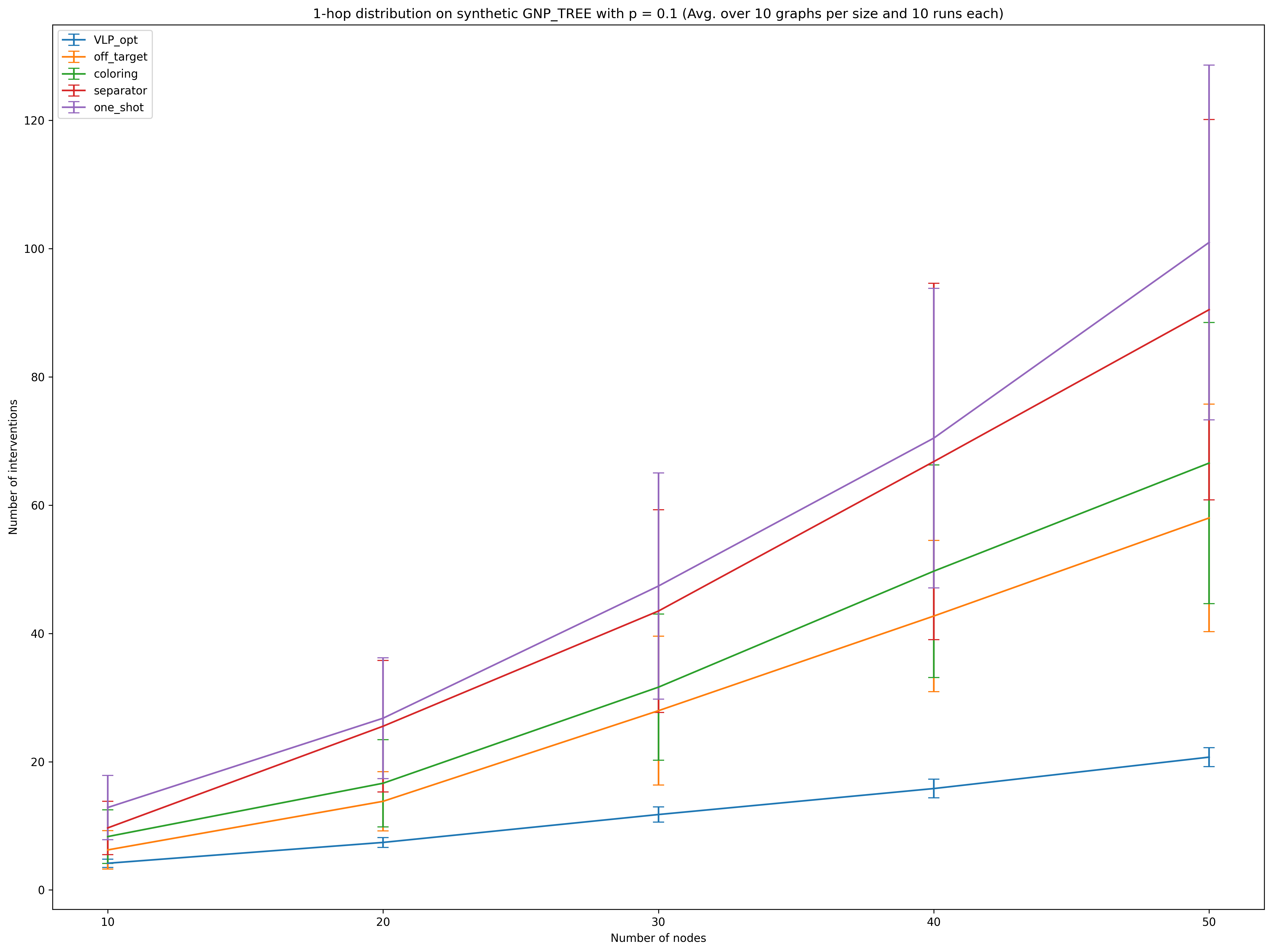
(a) 1-hop

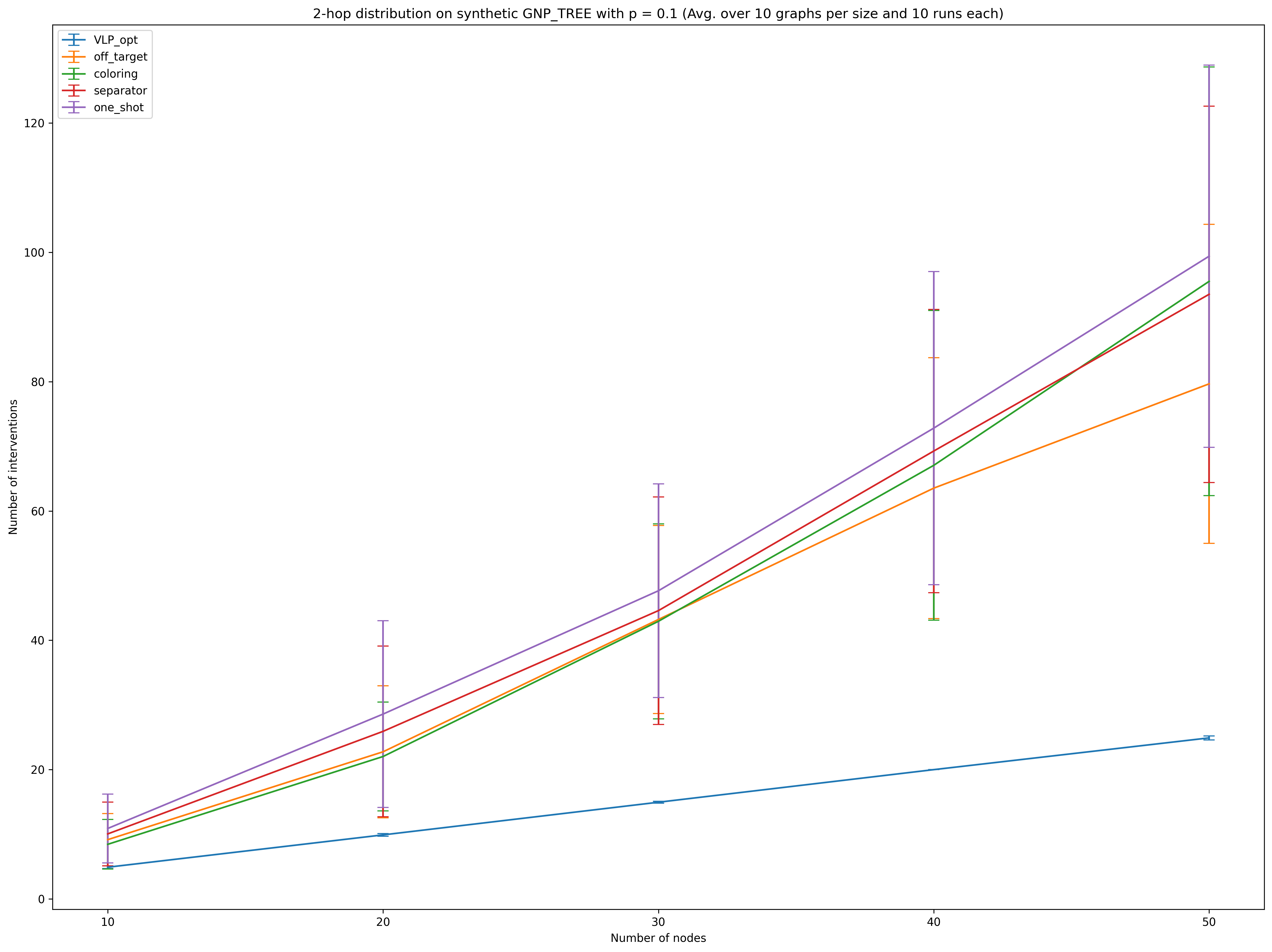
(b) 2-hop

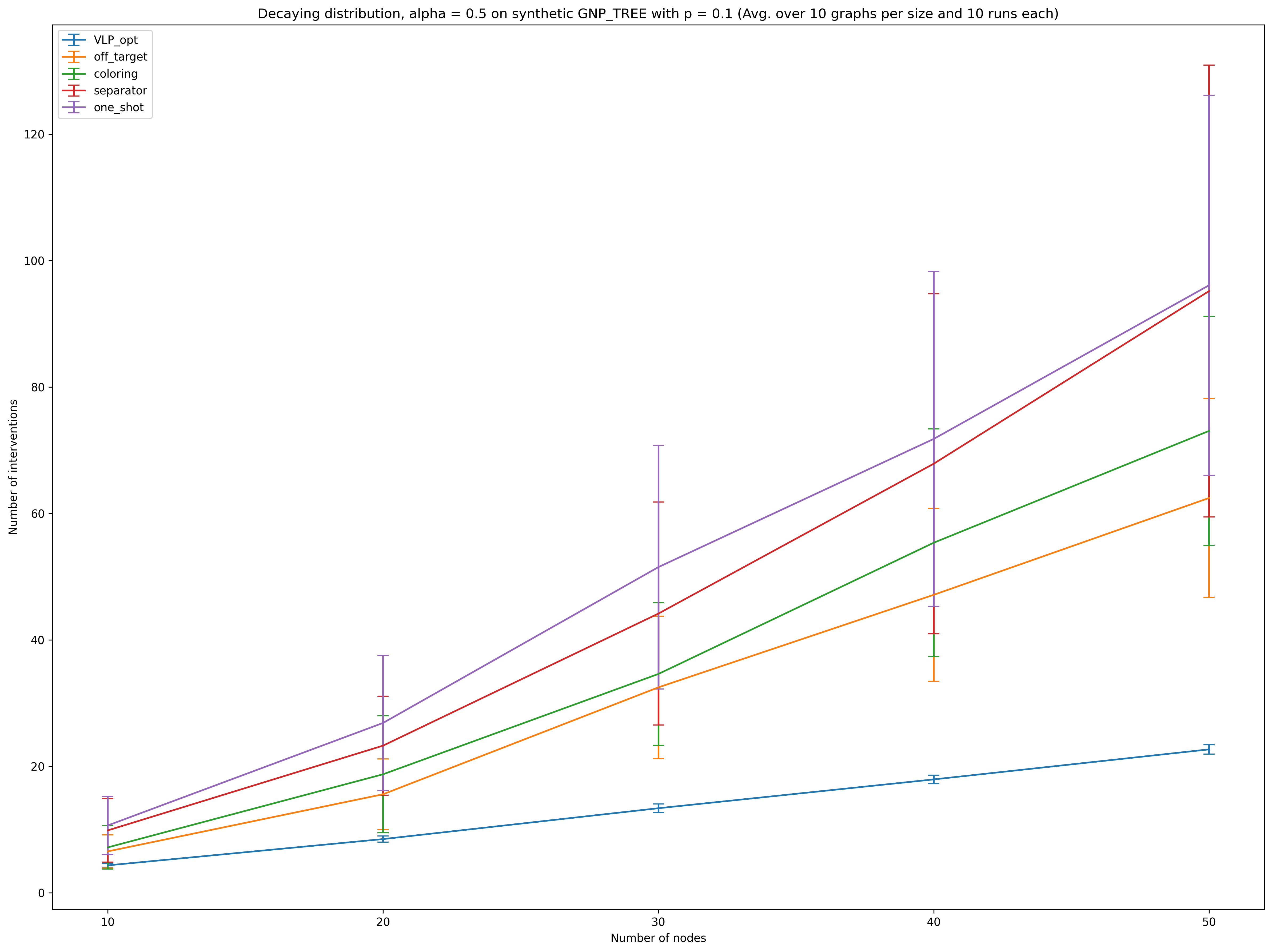
(c) Decaying, $\alpha=0.5$

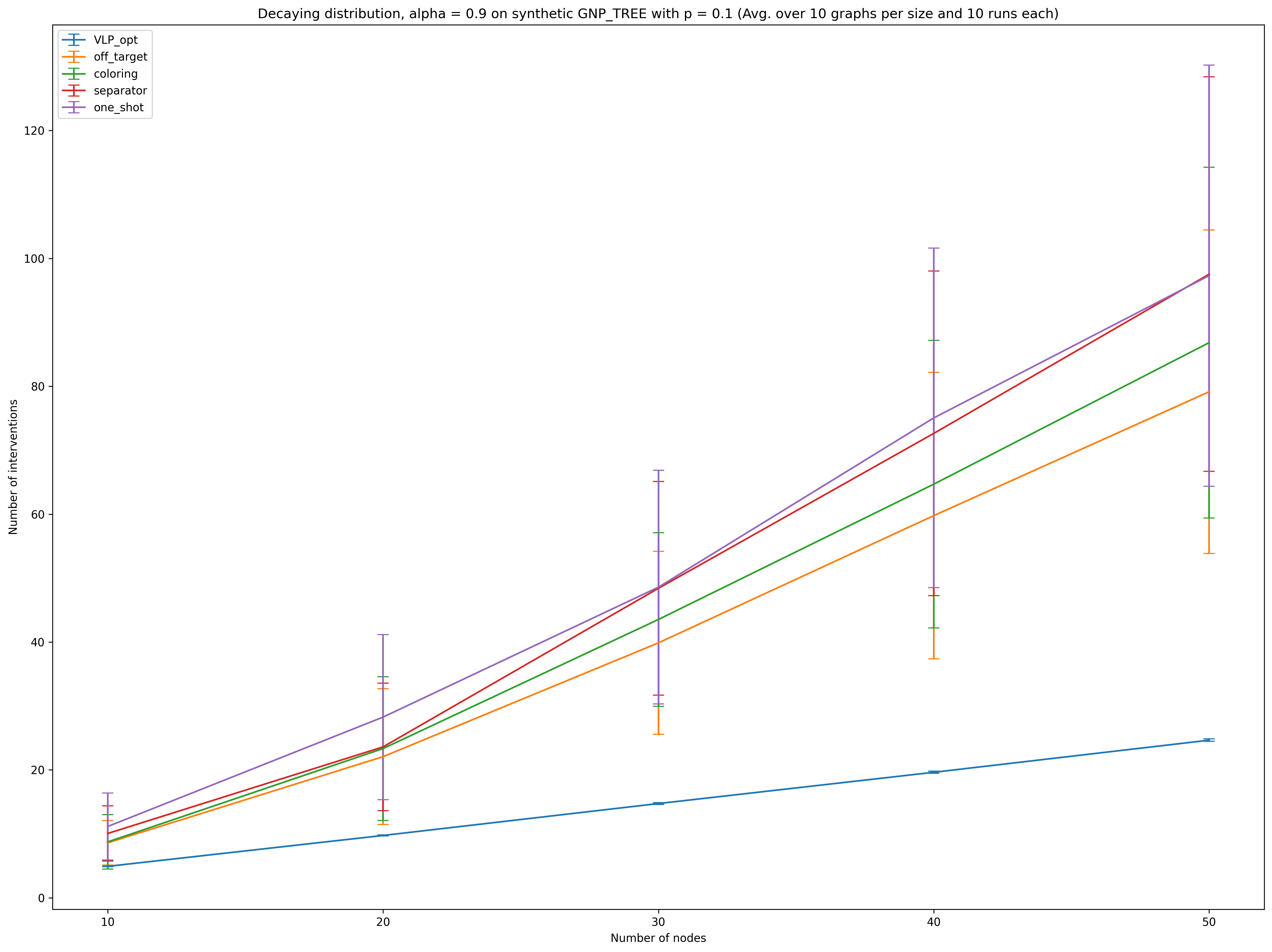
(d) Decaying, $\alpha=0.9$

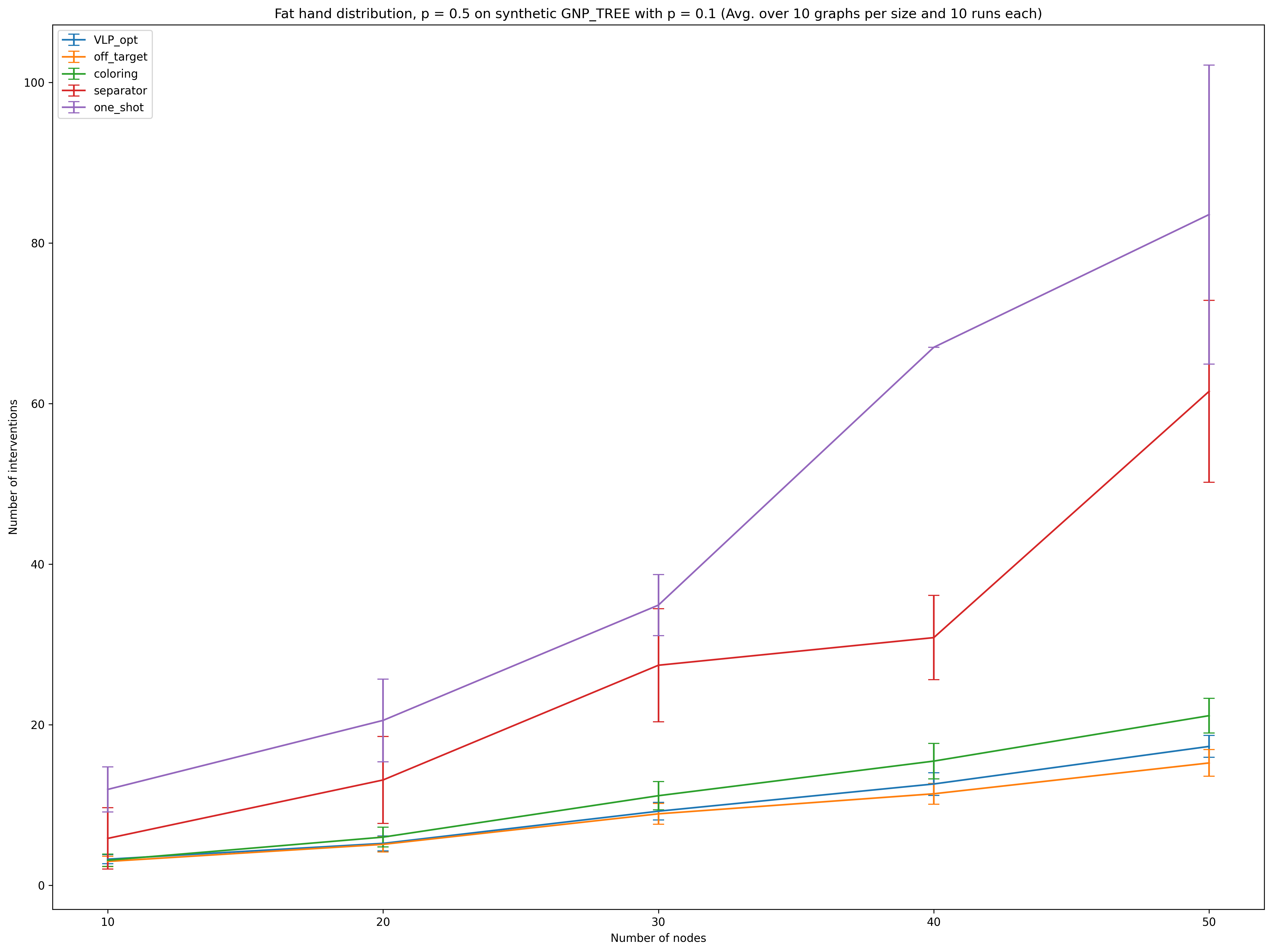
(e) Fat hand, $p=0.5$

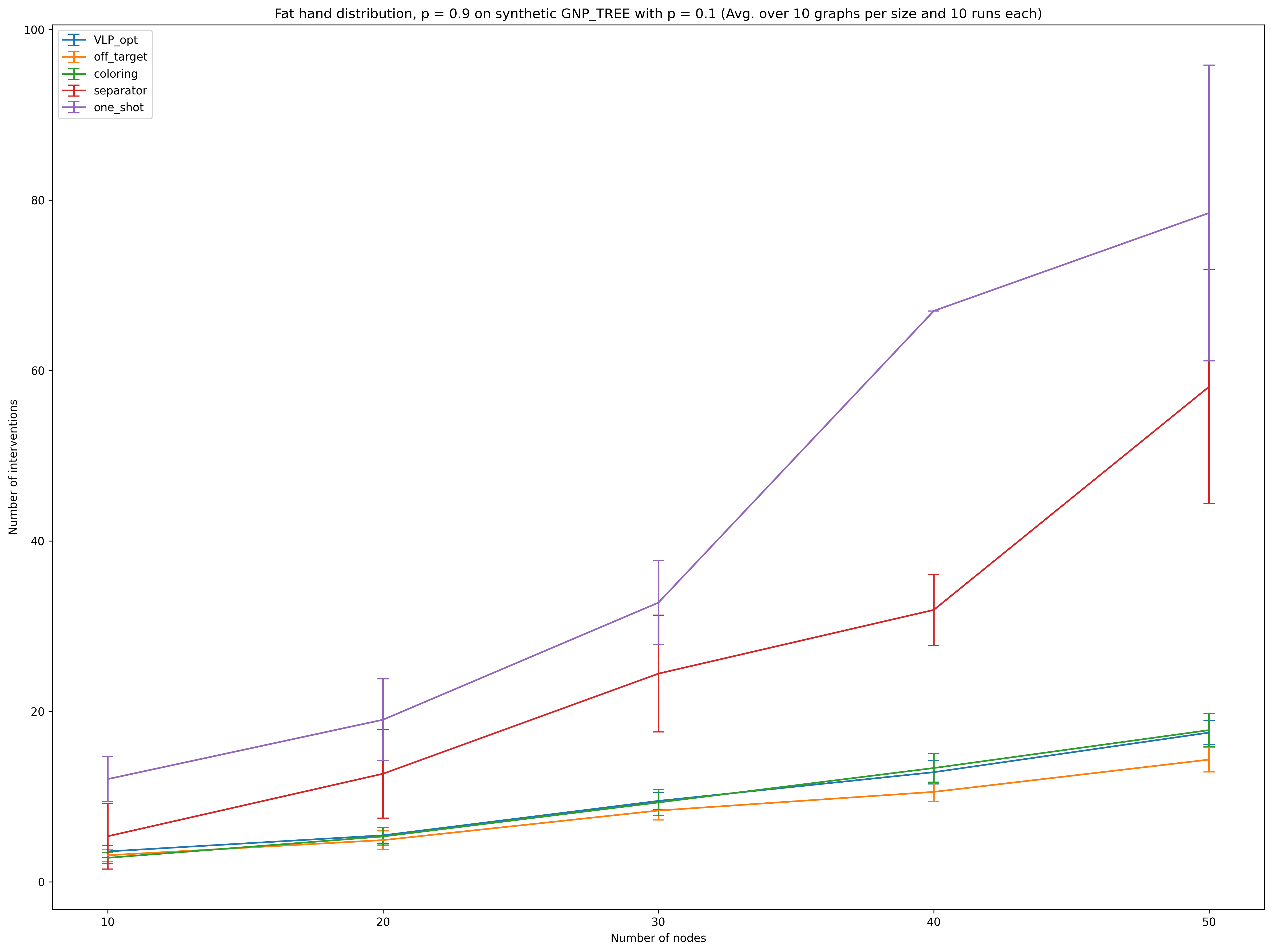
(f) Fat hand, $p=0.9$

Figure 6: GNP_TREE graphs without “random”. The optimal value of VLP in blue is an $\mathcal{O}(\log n)$ approximation of $\nu(G^{*})$. Our off-target search Off-Target is in orange. Coloring is in green. Separator is in red. One-shot is in purple.

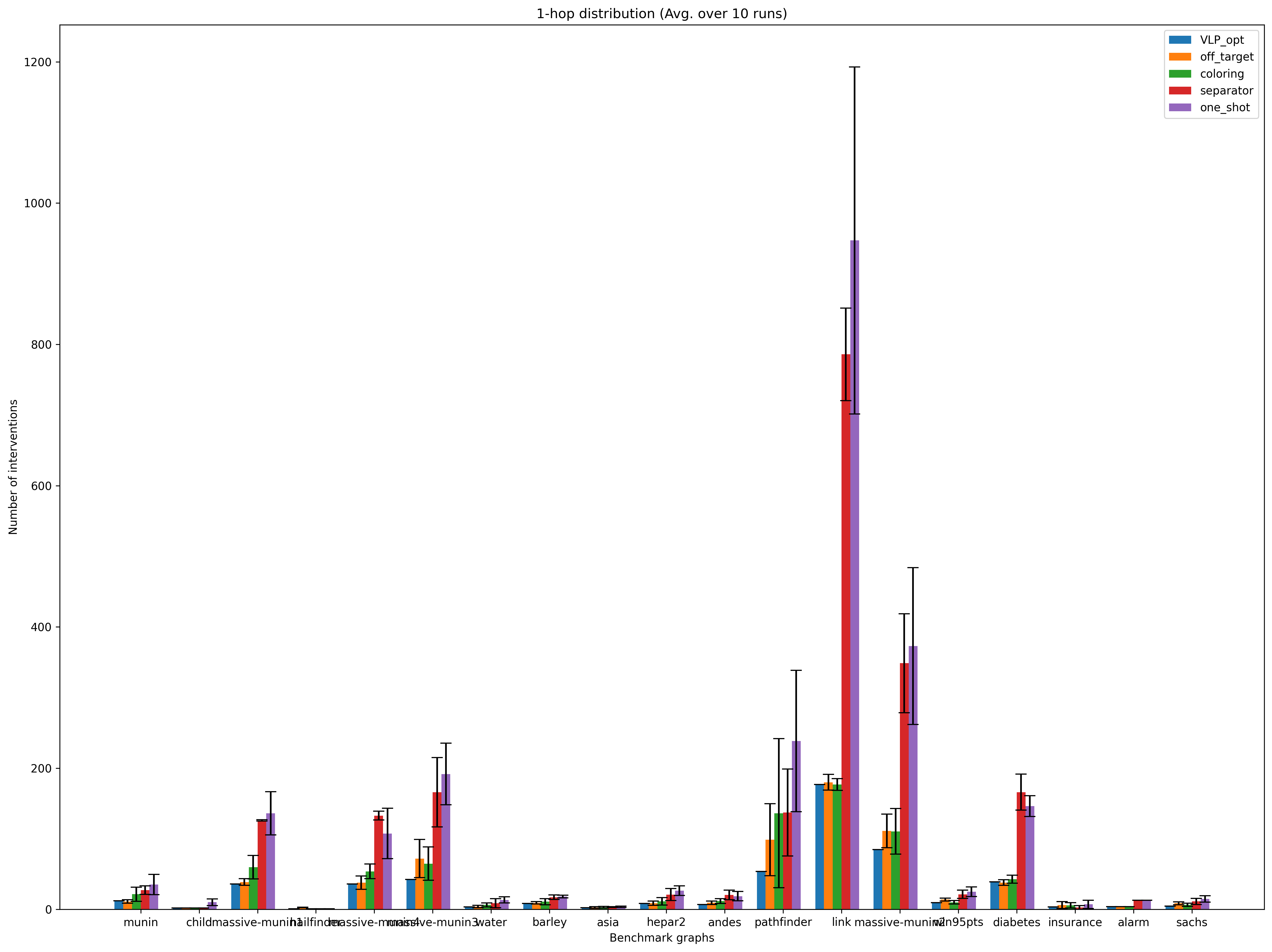
(a) 1-hop

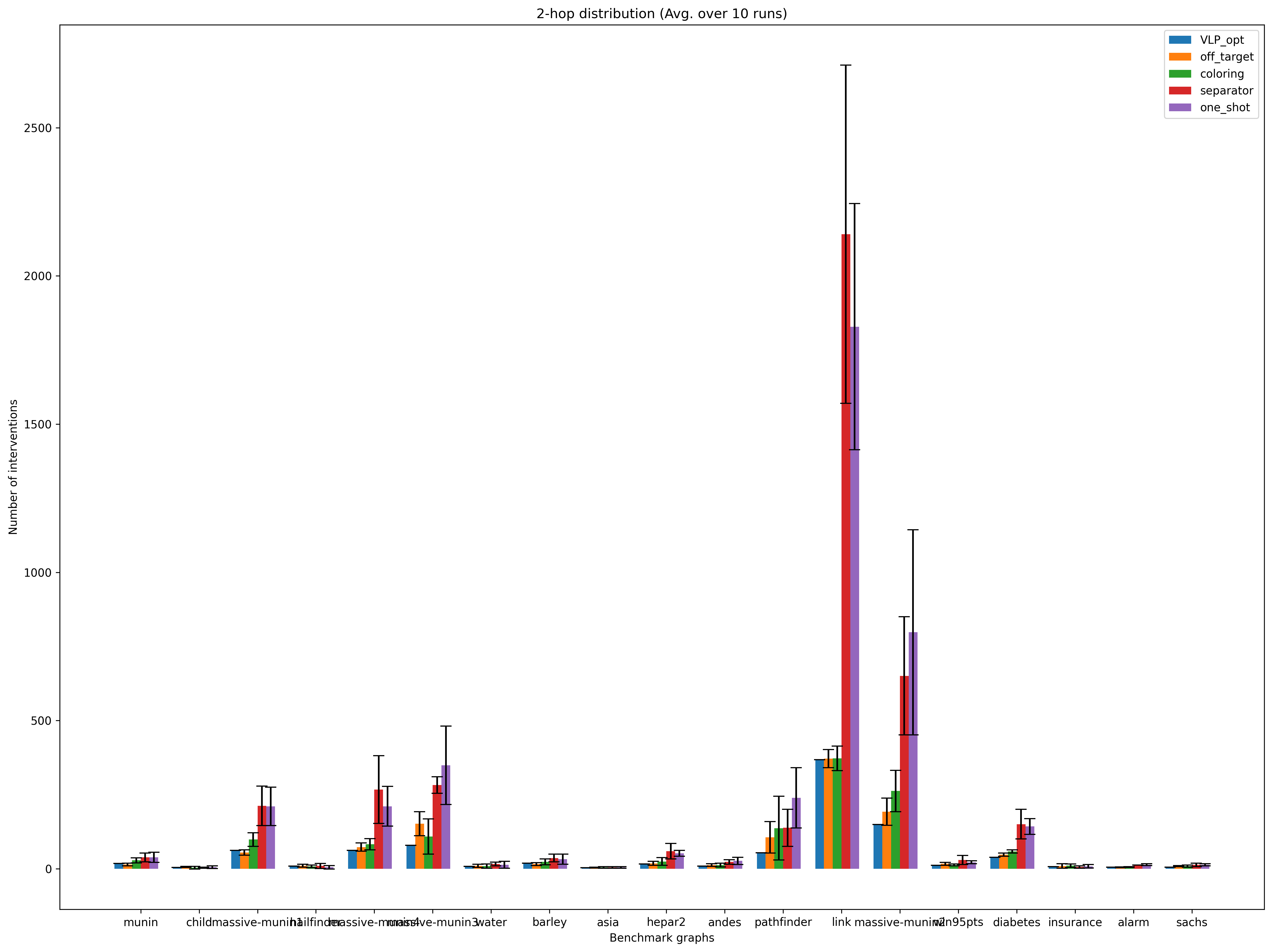
(b) 2-hop

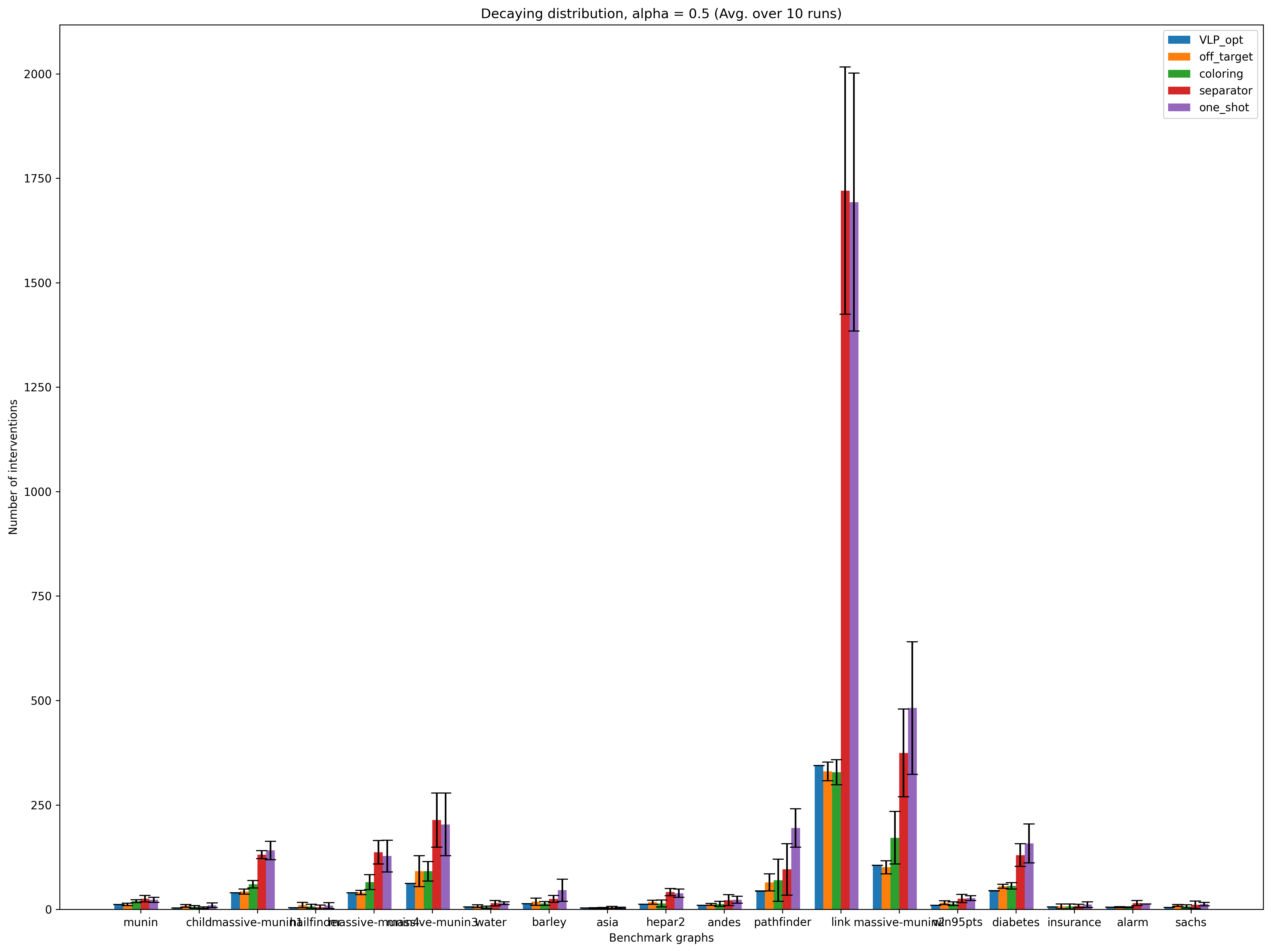
(c) Decaying, $\alpha=0.5$

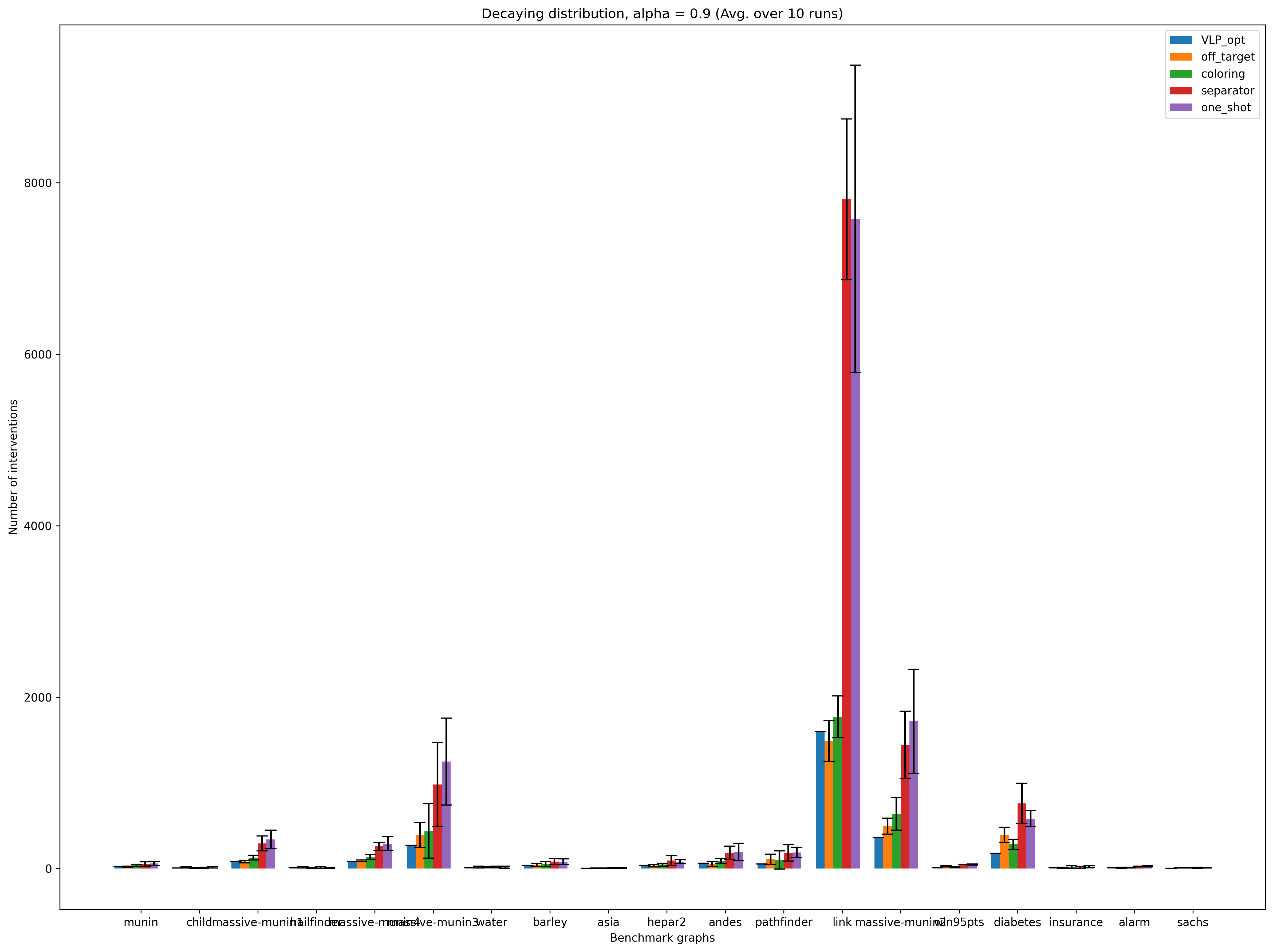
(d) Decaying, $\alpha=0.9$

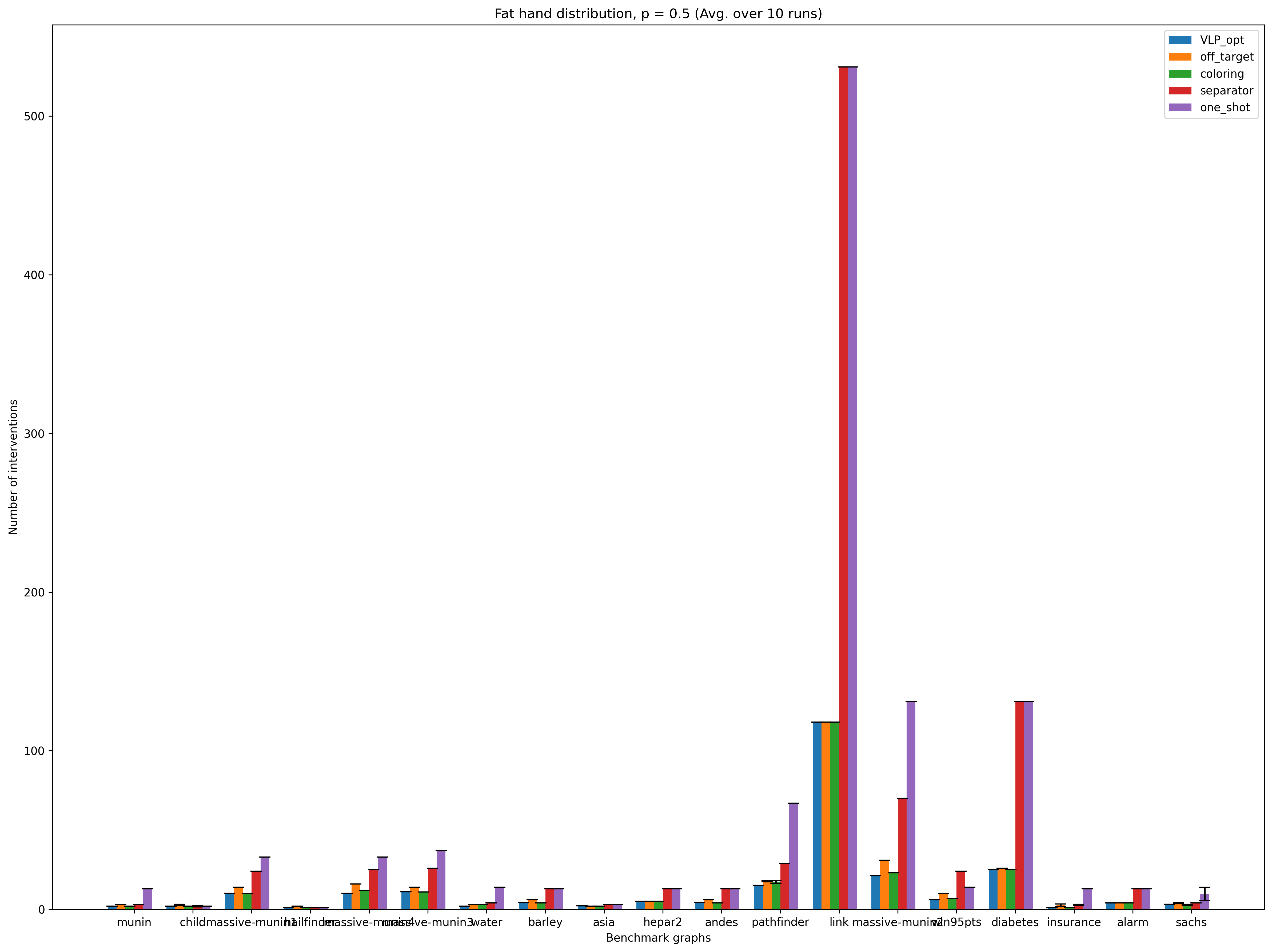
(e) Fat hand, $p=0.5$

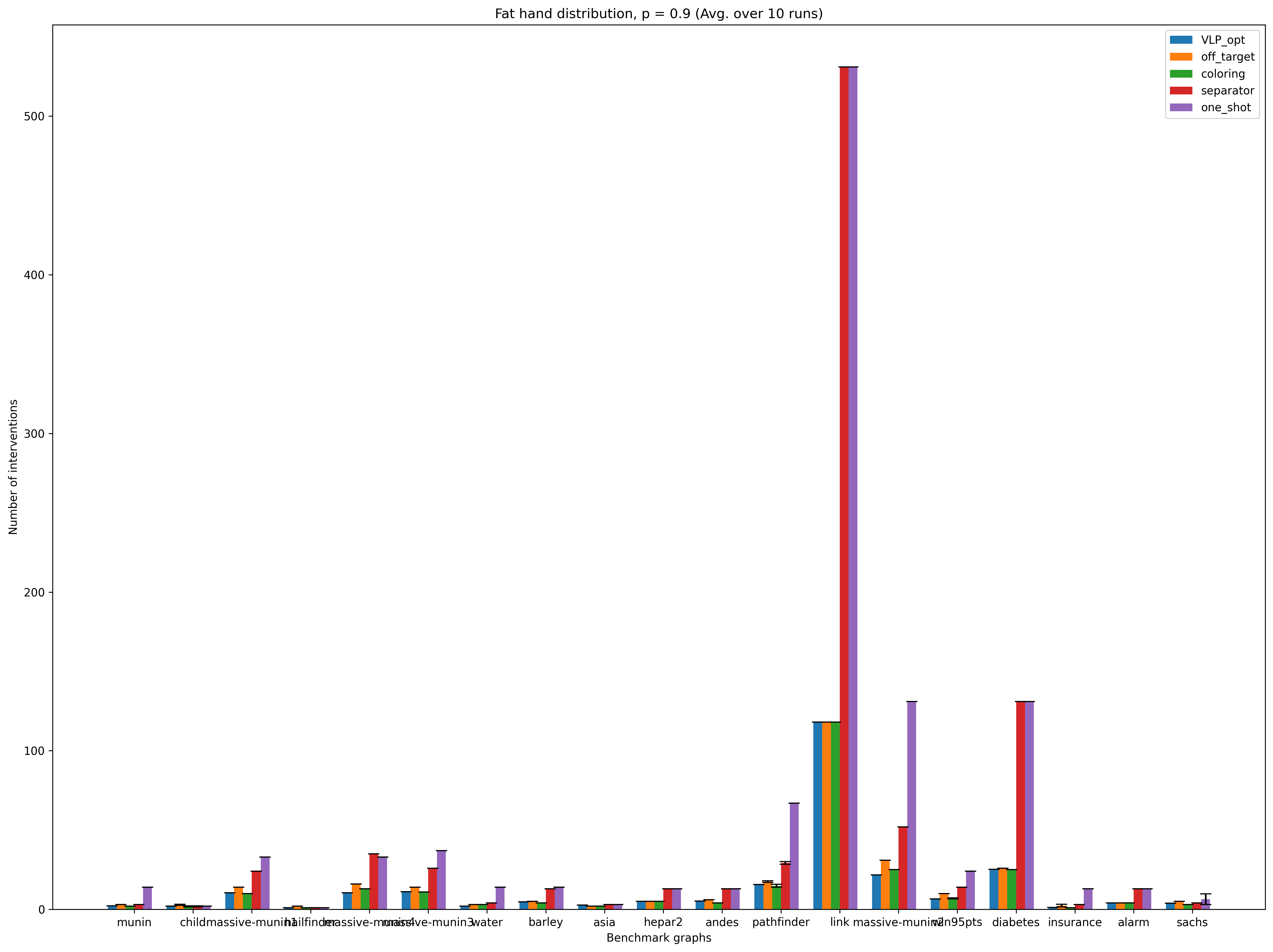
(f) Fat hand, $p=0.9$

Figure 7: bnlearn graphs without “random”. The optimal value of VLP in blue is an $\mathcal{O}(\log n)$ approximation of $\nu(G^{*})$. Our off-target search Off-Target is in orange. Coloring is in green. Separator is in red. One-shot is in purple.

E.5.2 Plots (with “random”)

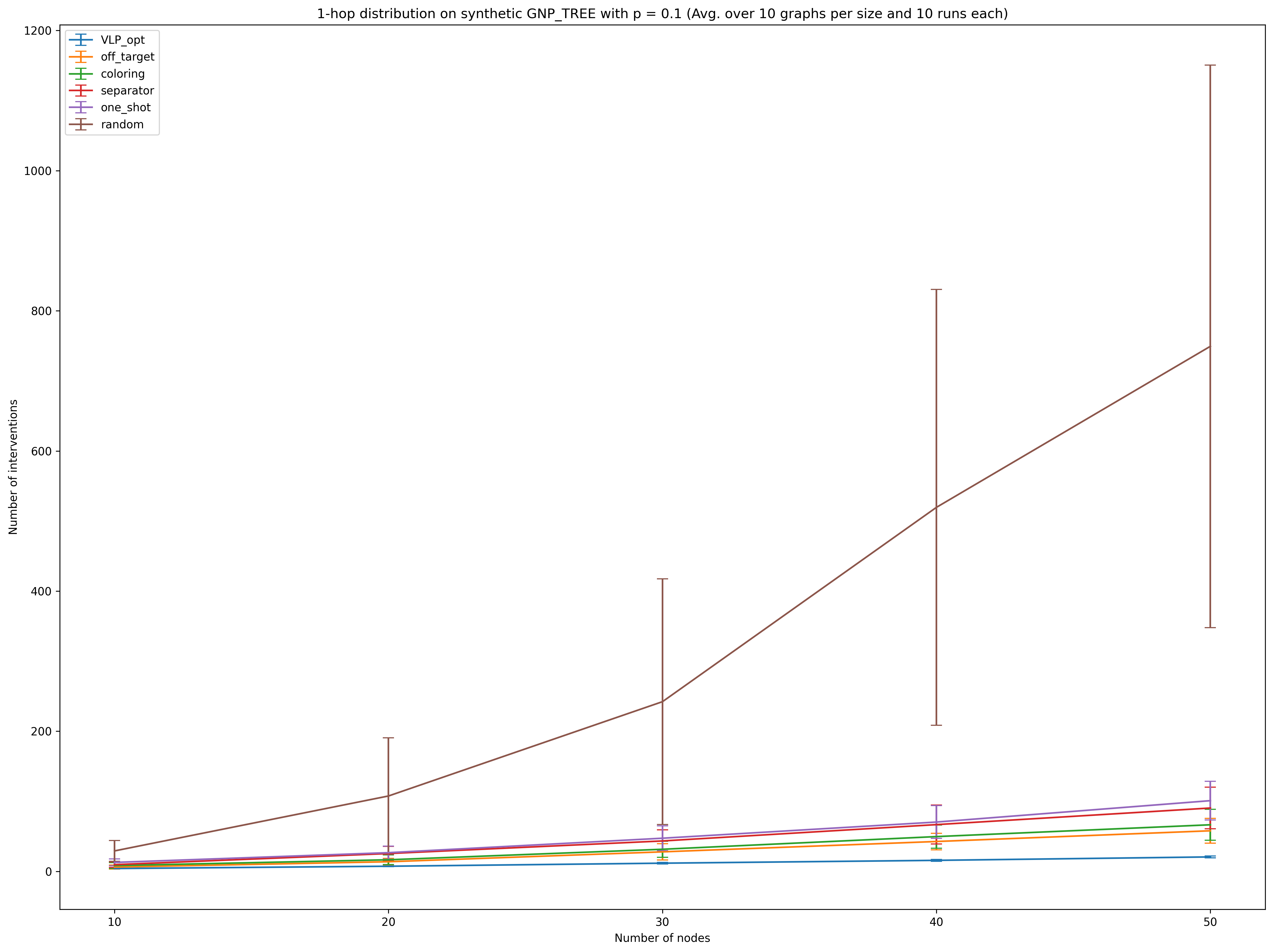
(a) 1-hop

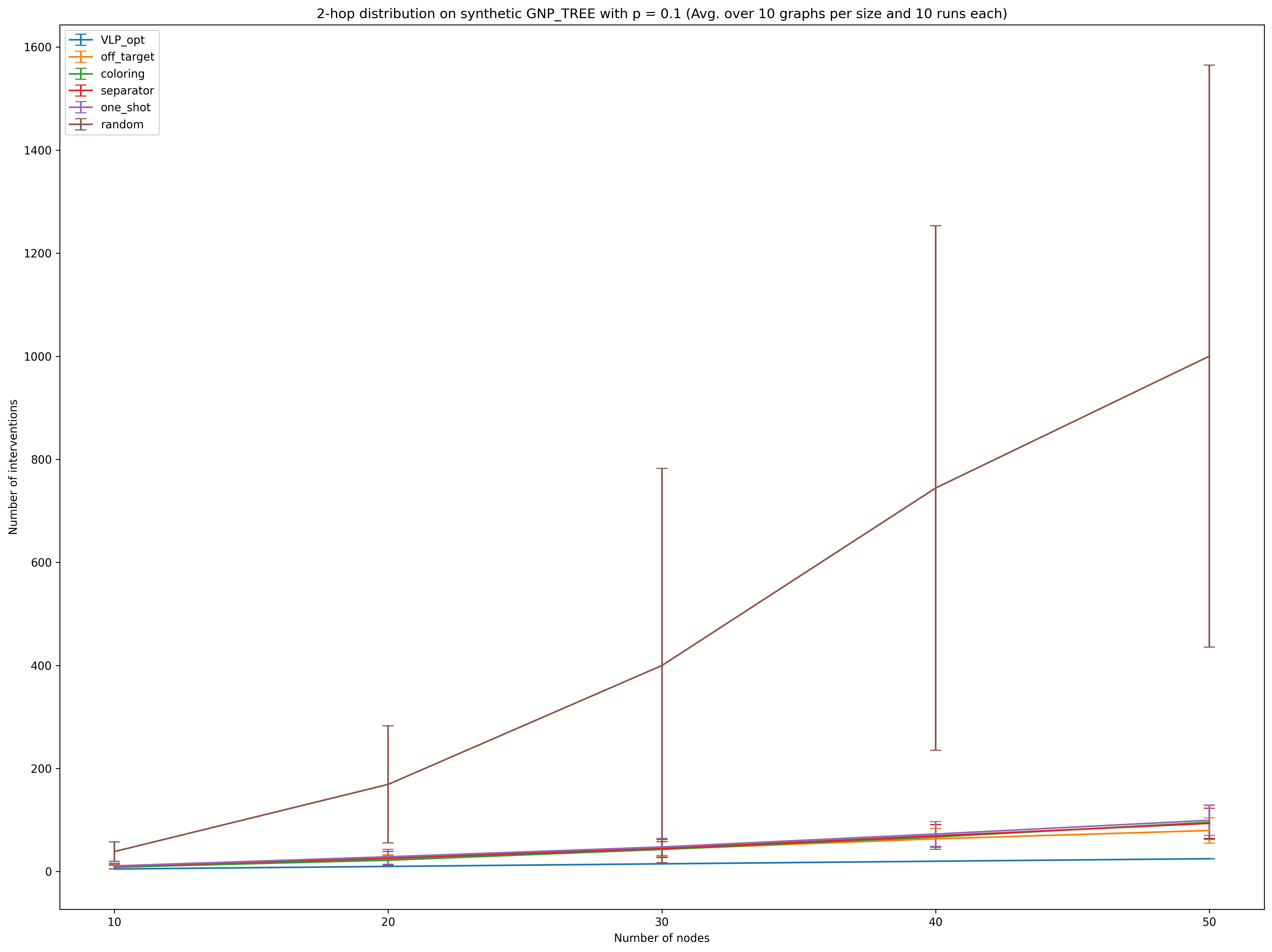
(b) 2-hop

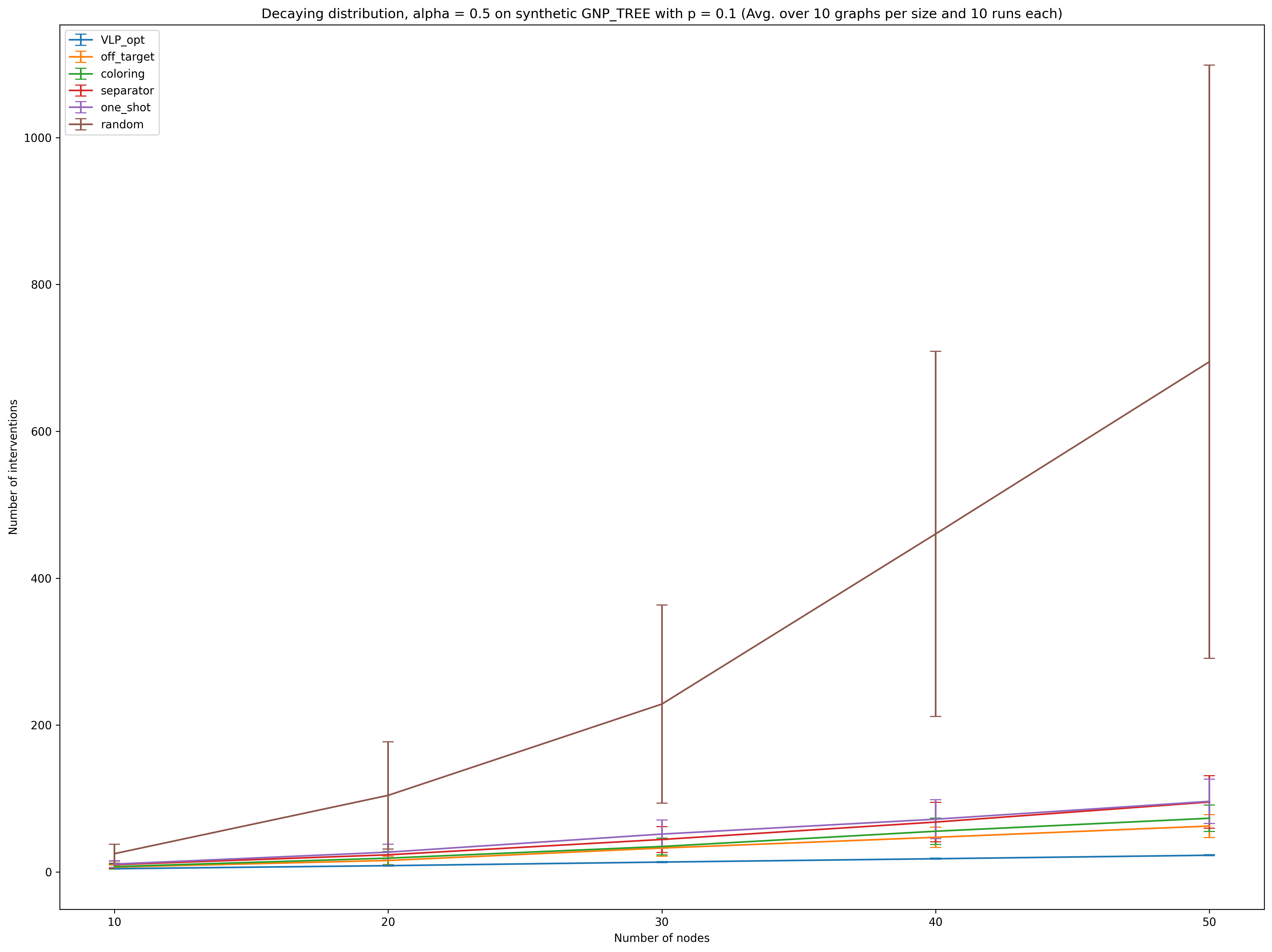
(c) Decaying, $\alpha=0.5$

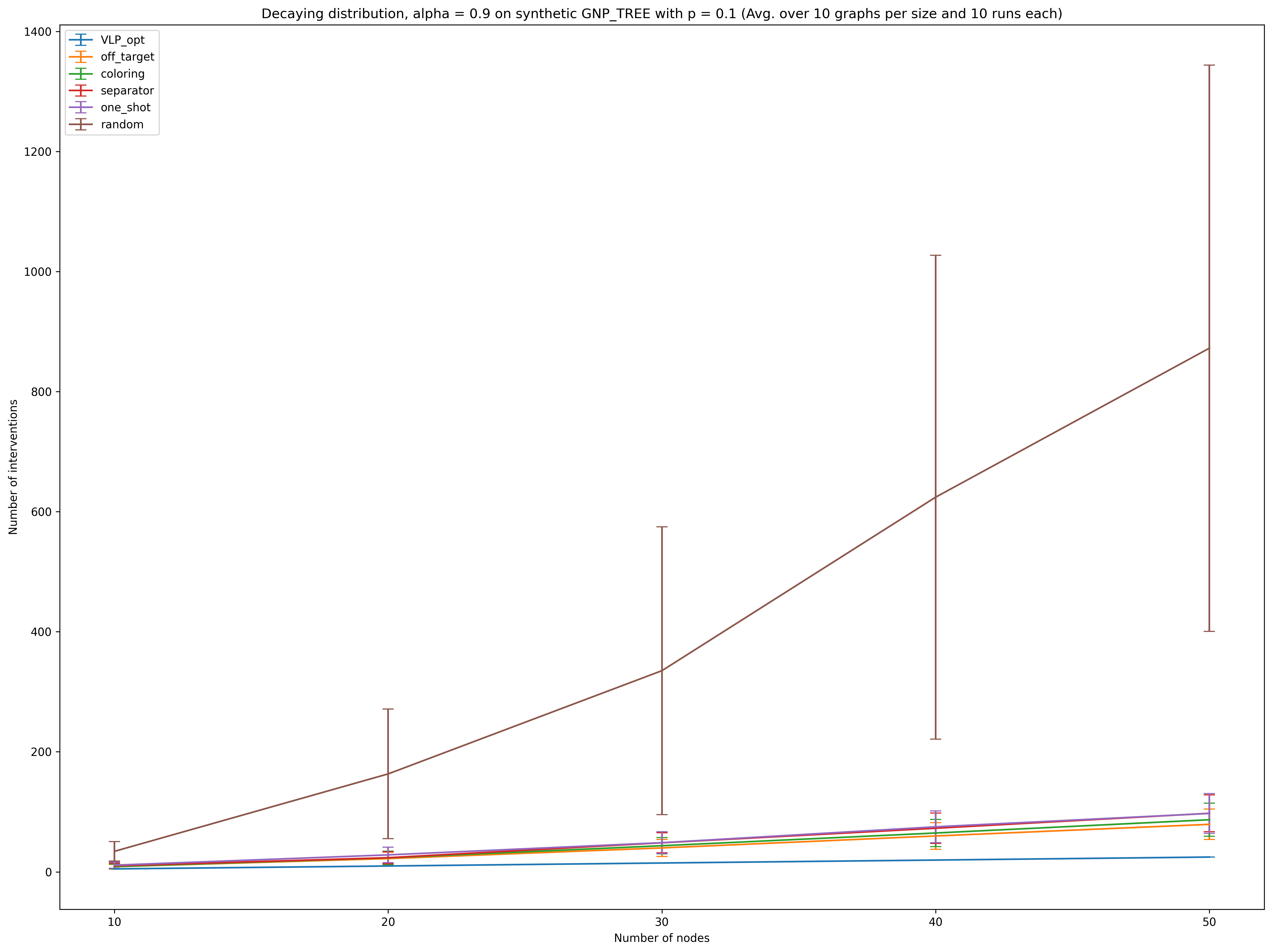
(d) Decaying, $\alpha=0.9$

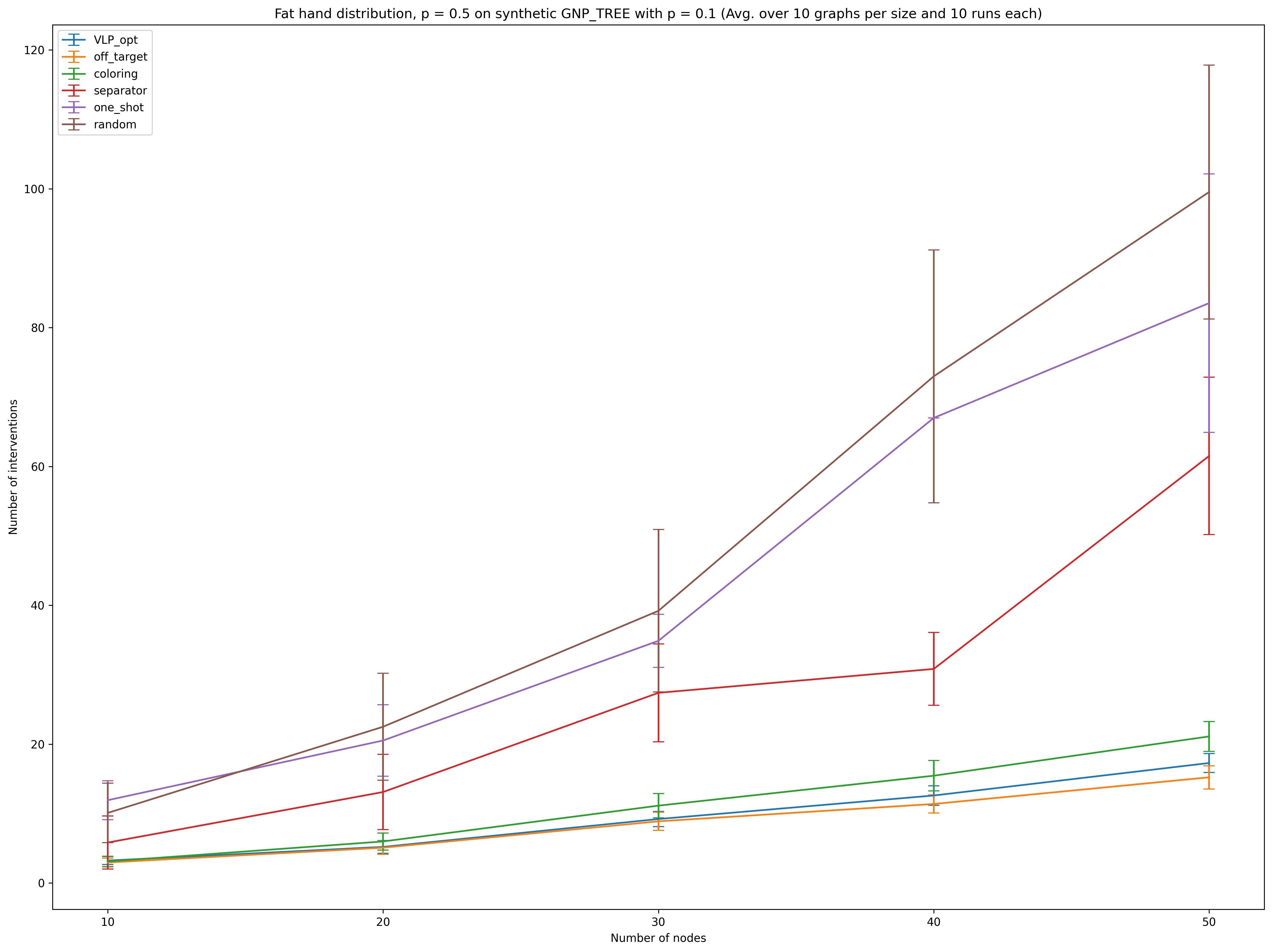
(e) Fat hand, $p=0.5$

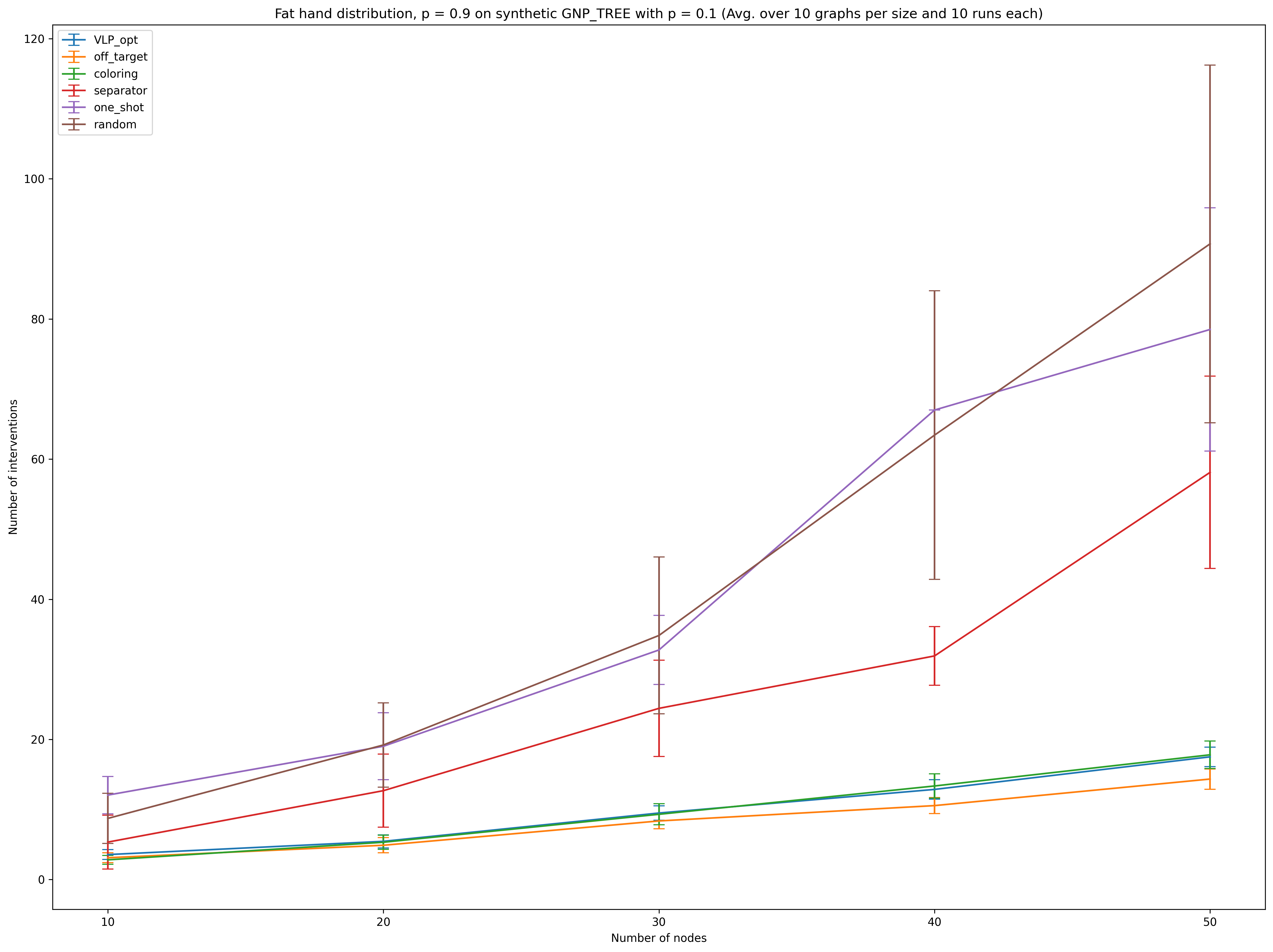
(f) Fat hand, $p=0.9$

Figure 8: GNP_TREE graphs. The optimal value of VLP in blue is an $\mathcal{O}(\log n)$ approximation of $\nu(G^{*})$. Our off-target search Off-Target is in orange. Coloring is in green. Separator is in red. One-shot is in purple. Random is in brown.

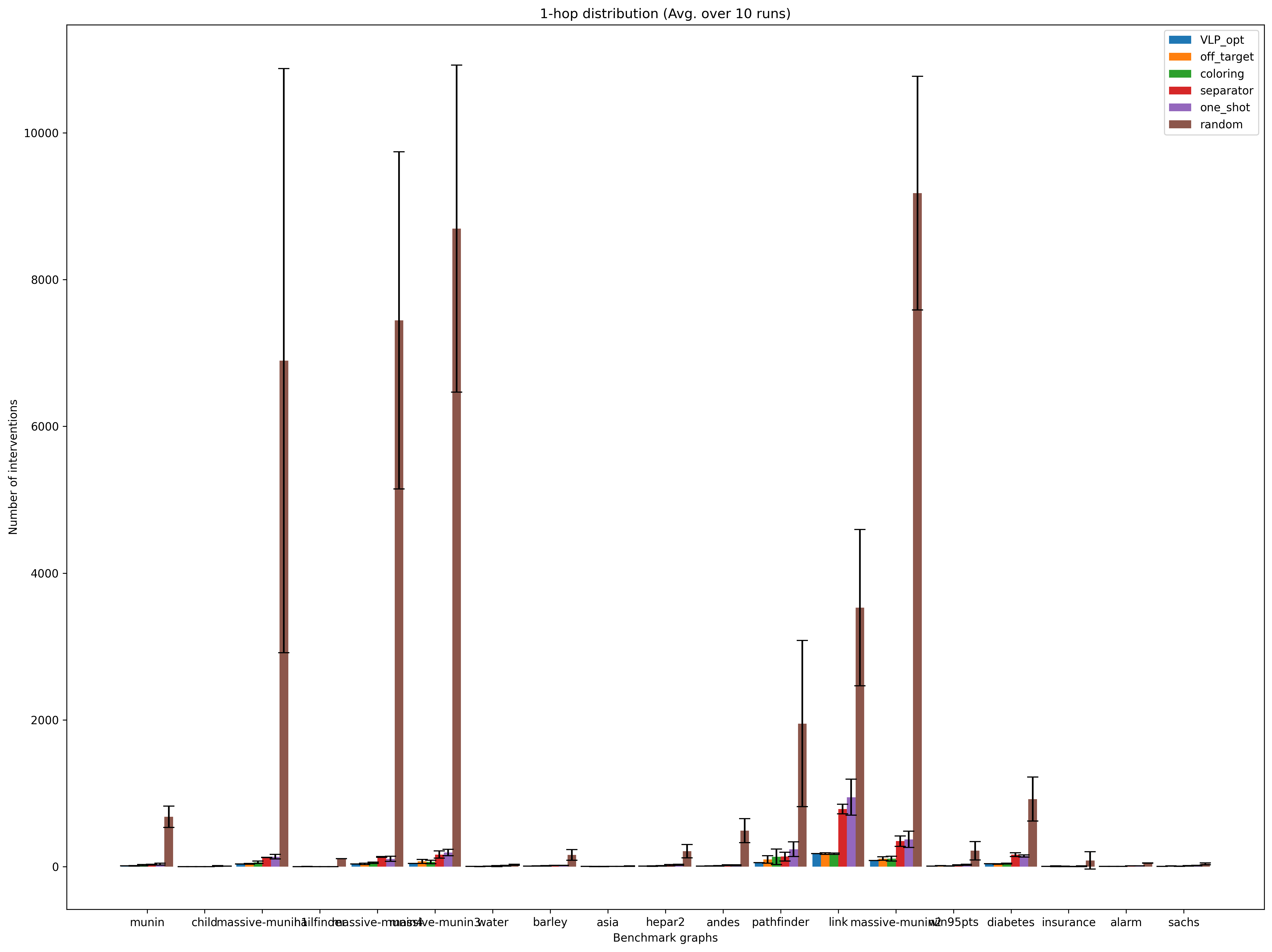
(a) 1-hop

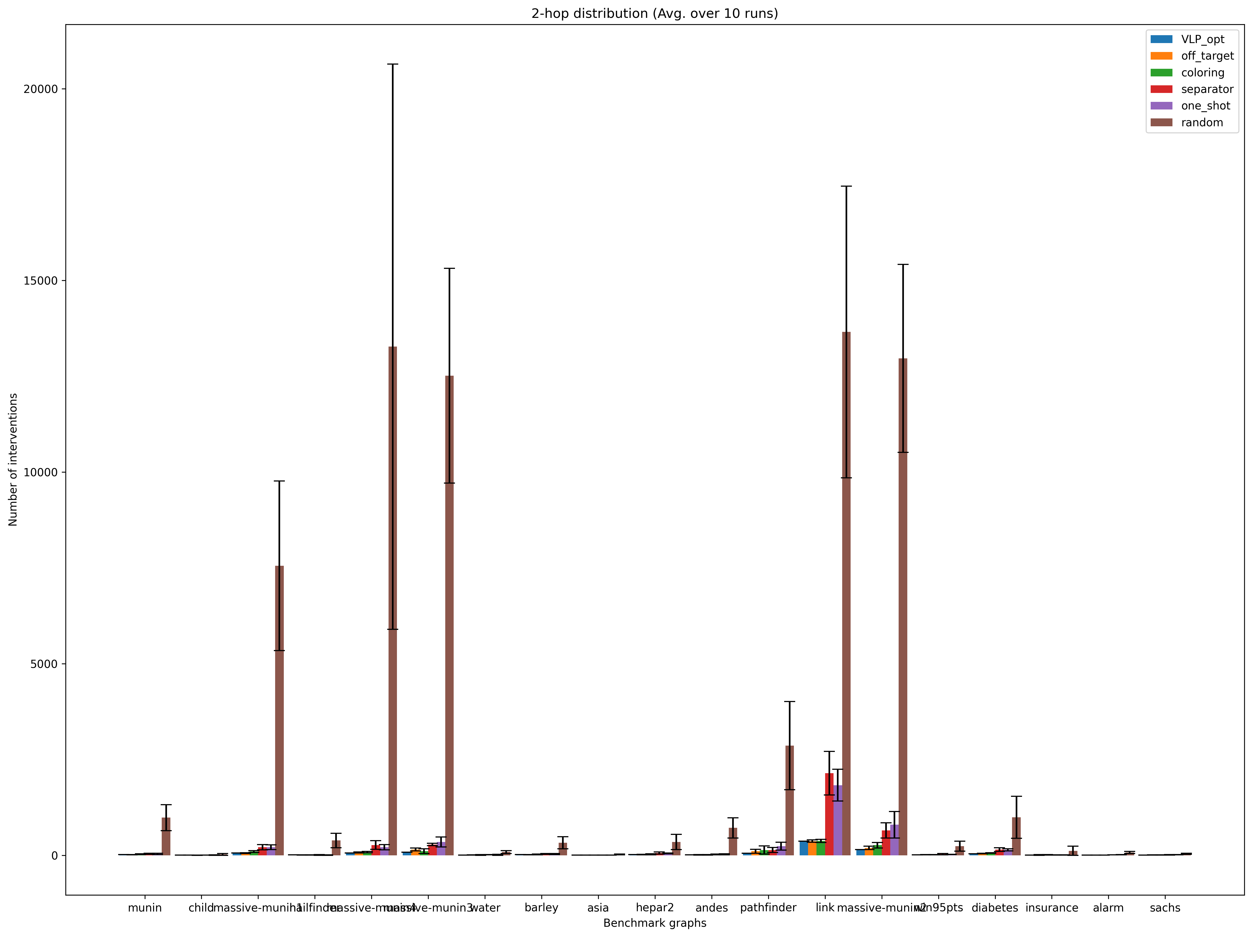
(b) 2-hop

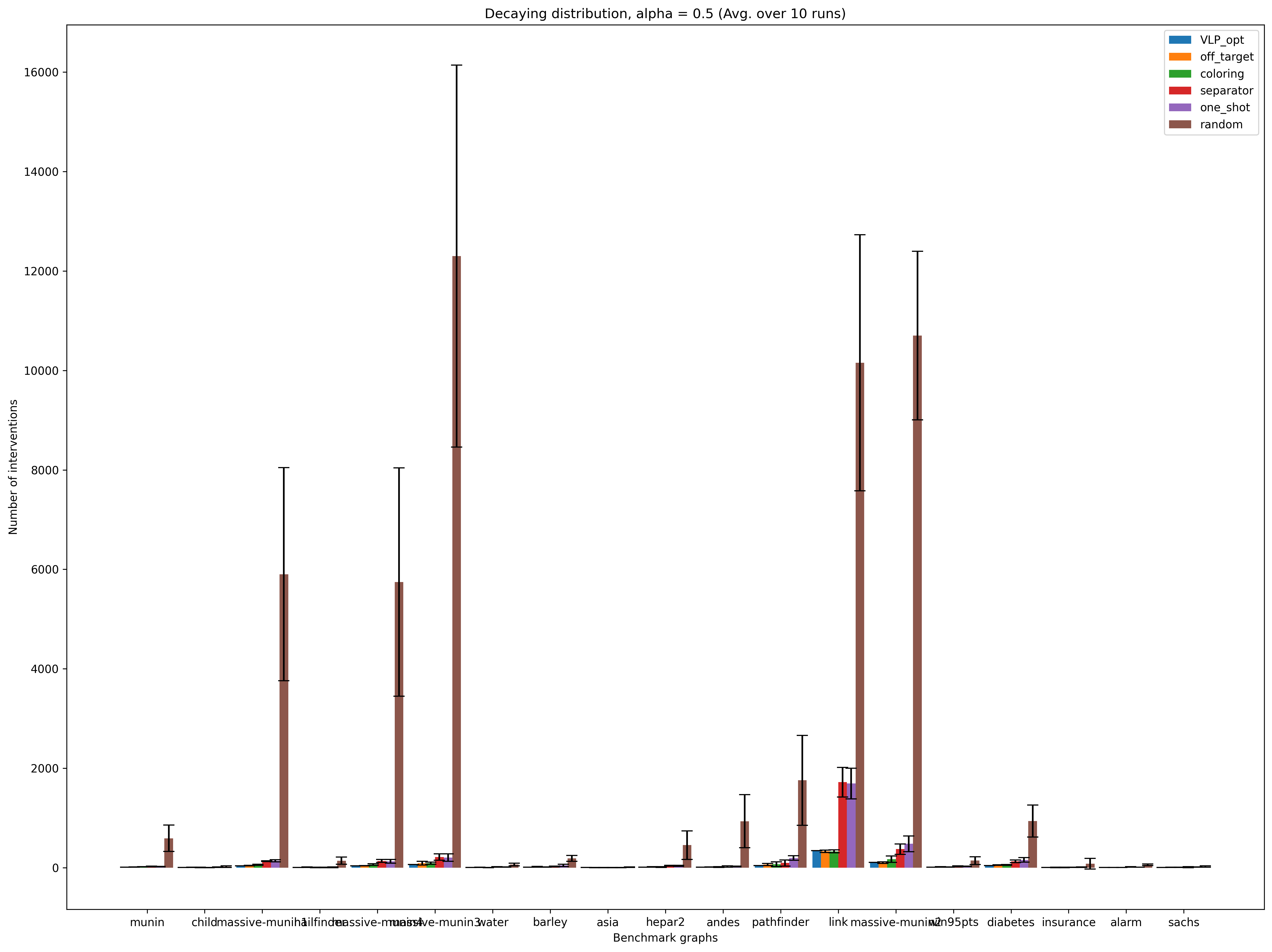
(c) Decaying, $\alpha=0.5$

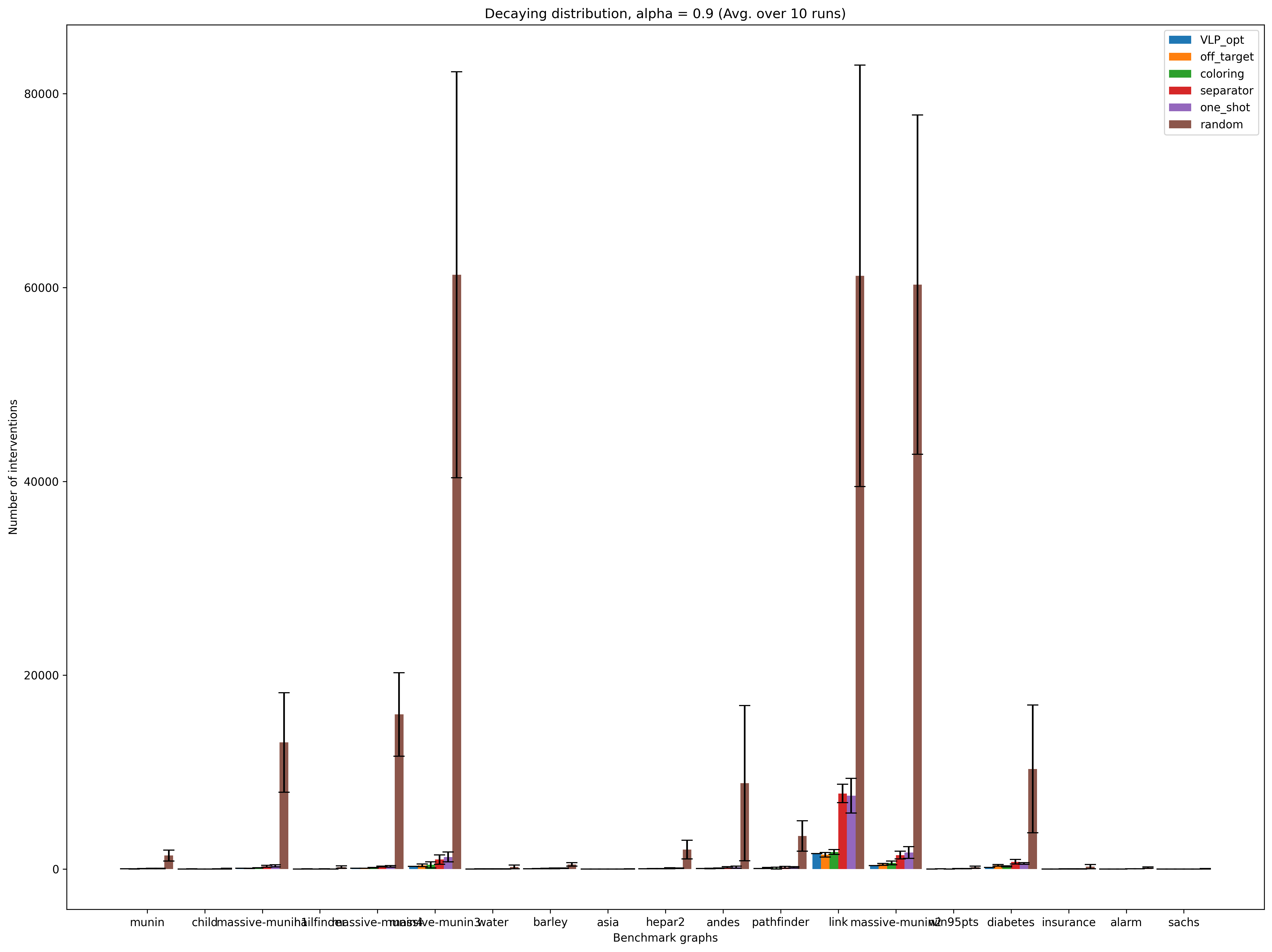
(d) Decaying, $\alpha=0.9$

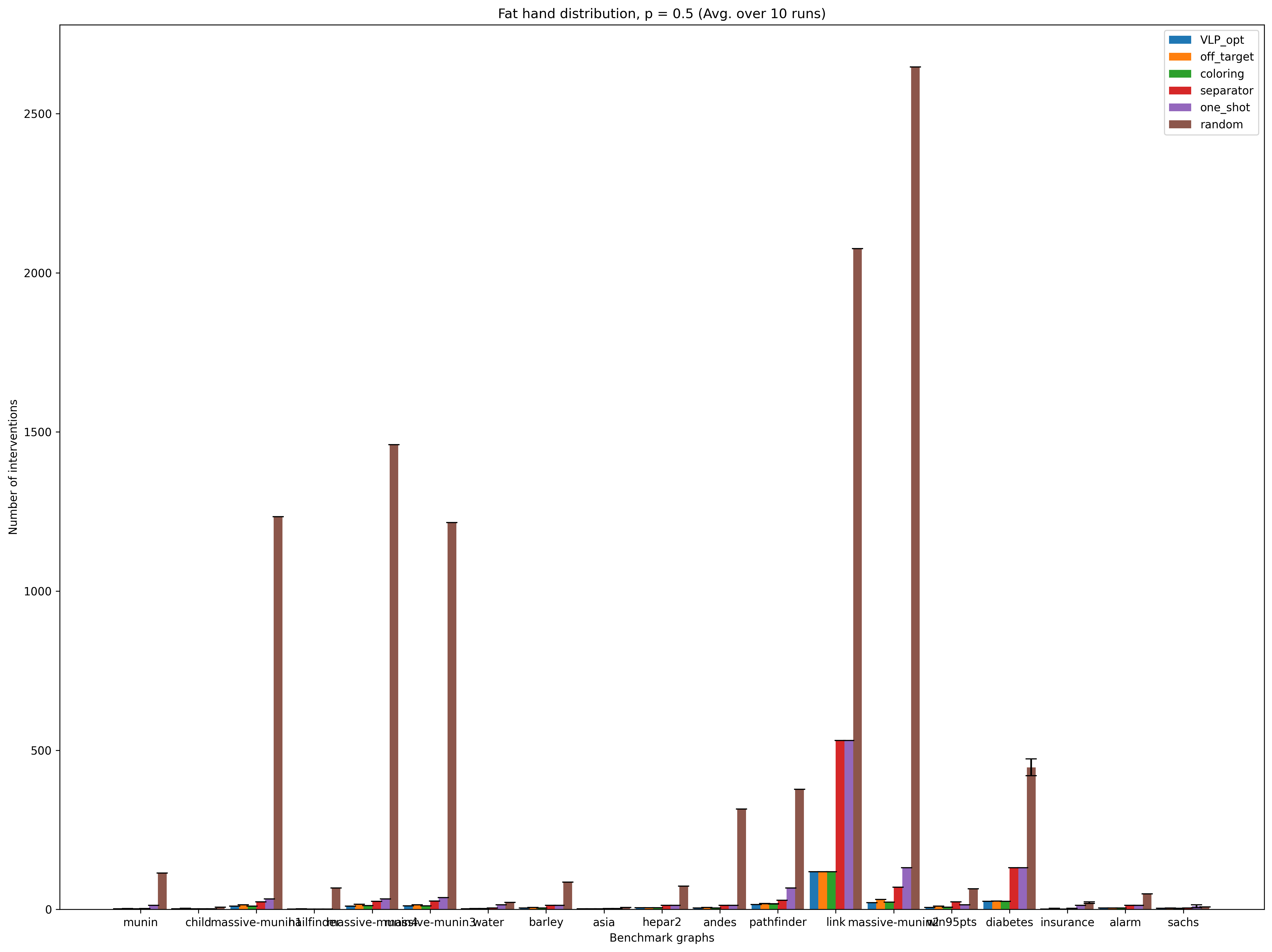
(e) Fat hand, $p=0.5$

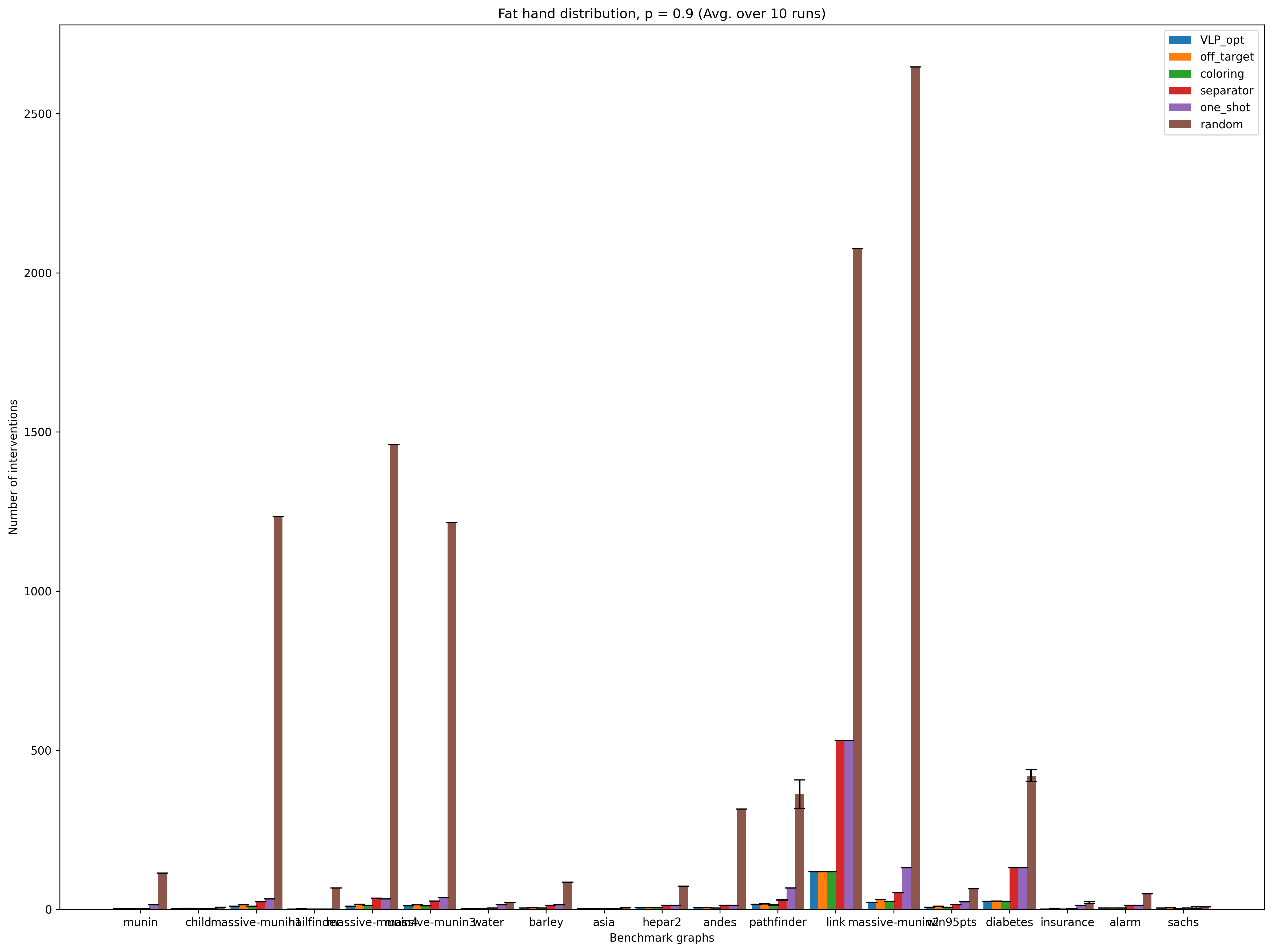
(f) Fat hand, $p=0.9$

Figure 9: bnlearn graphs. The optimal value of VLP in blue is an $\mathcal{O}(\log n)$ approximation of $\nu(G^{*})$. Our off-target search Off-Target is in orange. Coloring is in green. Separator is in red. One-shot is in purple. Random is in brown.

References

- [AMP97] Steen A. Andersson, David Madigan, and Michael D. Perlman. A characterization of Markov equivalence classes for acyclic digraphs. The Annals of Statistics, 25(2):505–541, 1997.
- [ASY+19] Raj Agrawal, Chandler Squires, Karren Yang, Karthikeyan Shanmugam, and Caroline Uhler. ABCD-Strategy: Budgeted Experimental Design for Targeted Causal Structure Discovery. In International Conference on Artificial Intelligence and Statistics, pages 3400–3409. PMLR, 2019.
- [AWL18] Neeraj K Aryal, Amanda R Wasylishen, and Guillermina Lozano. Crispr/cas9 can mediate high-efficiency off-target mutations in mice in vivo. Cell death & disease, 9(11):1099, 2018.
- [BP93] Jean R. S. Blair and Barry W. Peyton. An introduction to chordal graphs and clique trees. In Graph theory and sparse matrix computation, pages 1–29. Springer, 1993.
- [CBP16] Hyunghoon Cho, Bonnie Berger, and Jian Peng. Reconstructing Causal Biological Networks through Active Learning. PLoS ONE, 11(3):e0150611, 2016.
- [Chi95] David Maxwell Chickering. A Transformational Characterization of Equivalent Bayesian Network Structures. In Proceedings of the Eleventh Conference on Uncertainty in Artificial Intelligence, UAI’95, page 87–98, San Francisco, CA, USA, 1995. Morgan Kaufmann Publishers Inc.
- [CMKR12] Diego Colombo, Marloes H. Maathuis, Markus Kalisch, and Thomas S. Richardson. Learning high-dimensional directed acyclic graphs with latent and selection variables. The Annals of Statistics, pages 294–321, 2012.
- [CS23a] Davin Choo and Kirankumar Shiragur. New metrics and search algorithms for weighted causal DAGs. International Conference on Machine Learning, 2023.
- [CS23b] Davin Choo and Kirankumar Shiragur. Subset verification and search algorithms for causal DAGs. In International Conference on Artificial Intelligence and Statistics, 2023.
- [CSB22] Davin Choo, Kirankumar Shiragur, and Arnab Bhattacharyya. Verification and search algorithms for causal DAGs. Advances in Neural Information Processing Systems, 35, 2022.
- [CY99] Gregory F. Cooper and Changwon Yoo. Causal Discovery from a Mixture of Experimental and Observational Data. In Proceedings of the Fifteenth conference on Uncertainty in artificial intelligence, pages 116–125, 1999.
- [dCCCM19] Luis M. de Campos, Andrés Cano, Javier G. Castellano, and Serafín Moral. Combining gene expression data and prior knowledge for inferring gene regulatory networks via Bayesian networks using structural restrictions. Statistical Applications in Genetics and Molecular Biology, 18(3), 2019.
- [DEMS10] David Duvenaud, Daniel Eaton, Kevin Murphy, and Mark Schmidt. Causal learning without dags. In Causality: Objectives and Assessment, pages 177–190. PMLR, 2010.
- [DS14] Irit Dinur and David Steurer. Analytical approach to parallel repetition. In Proceedings of the forty-sixth annual ACM symposium on Theory of computing, pages 624–633, 2014.
- [Ebe07] Frederick Eberhardt. Causation and Intervention. Unpublished doctoral dissertation, Carnegie Mellon University, page 93, 2007.
- [Ebe10] Frederick Eberhardt. Causal Discovery as a Game. In Causality: Objectives and Assessment, pages 87–96. PMLR, 2010.
- [EGS05] Frederick Eberhardt, Clark Glymour, and Richard Scheines. On the number of experiments sufficient and in the worst case necessary to identify all causal relations among N variables. In Proceedings of the Twenty-First Conference on Uncertainty in Artificial Intelligence, pages 178–184, 2005.
- [EGS06] Frederick Eberhardt, Clark Glymour, and Richard Scheines. N-1 Experiments Suffice to Determine the Causal Relations Among N Variables. In Innovations in machine learning, pages 97–112. Springer, 2006.
- [EGS12] Frederick Eberhardt, Clark Glymour, and Richard Scheines. On the Number of Experiments Sufficient and in the Worst Case Necessary to Identify All Causal Relations Among N Variables. arXiv preprint arXiv:1207.1389, 2012.
- [EM07] Daniel Eaton and Kevin Murphy. Exact bayesian structure learning from uncertain interventions. In Artificial intelligence and statistics, pages 107–114. PMLR, 2007.
- [Ero20] Markus I Eronen. Causal discovery and the problem of psychological interventions. New Ideas in Psychology, 59:100785, 2020.
- [ES07] Frederick Eberhardt and Richard Scheines. Interventions and Causal Inference. Philosophy of science, 74(5):981–995, 2007.
- [FFK+13] Yanfang Fu, Jennifer A Foden, Cyd Khayter, Morgan L Maeder, Deepak Reyon, J Keith Joung, and Jeffry D Sander. High-frequency off-target mutagenesis induced by crispr-cas nucleases in human cells. Nature biotechnology, 31(9):822–826, 2013.
- [FK00] Nir Friedman and Daphne Koller. Being Bayesian about Network Structure. In Proceedings of the 16th Conference on Uncertainty in Artificial Intelligence, pages 201–210, 2000.
- [GK11] Daniel Golovin and Andreas Krause. Adaptive submodularity: Theory and applications in active learning and stochastic optimization. Journal of Artificial Intelligence Research, 42:427–486, 2011.
- [GKS+19] Kristjan Greenewald, Dmitriy Katz, Karthikeyan Shanmugam, Sara Magliacane, Murat Kocaoglu, Enric Boix-Adserà, and Guy Bresler. Sample Efficient Active Learning of Causal Trees. Advances in Neural Information Processing Systems, 32, 2019.
- [GRE84] John R. Gilbert, Donald J. Rose, and Anders Edenbrandt. A Separator Theorem for Chordal Graphs. SIAM Journal on Algebraic Discrete Methods, 5(3):306–313, 1984.
- [GS17] M Maria Glymour and Donna Spiegelman. Evaluating public health interventions: 5. causal inference in public health research—do sex, race, and biological factors cause health outcomes? American journal of public health, 107(1):81–85, 2017.
- [GSKB18] AmirEmad Ghassami, Saber Salehkaleybar, Negar Kiyavash, and Elias Bareinboim. Budgeted Experiment Design for Causal Structure Learning. In International Conference on Machine Learning, pages 1724–1733. PMLR, 2018.
- [GV06] Michel Goemans and Jan Vondrák. Stochastic covering and adaptivity. In LATIN 2006: Theoretical Informatics: 7th Latin American Symposium, Valdivia, Chile, March 20-24, 2006. Proceedings 7, pages 532–543. Springer, 2006.
- [GZS19] Clark Glymour, Kun Zhang, and Peter Spirtes. Review of causal discovery methods based on graphical models. Frontiers in genetics, 10:524, 2019.
- [HB12] Alain Hauser and Peter Bühlmann. Characterization and greedy learning of interventional Markov equivalence classes of directed acyclic graphs. The Journal of Machine Learning Research, 13(1):2409–2464, 2012.
- [HB14] Alain Hauser and Peter Bühlmann. Two Optimal Strategies for Active Learning of Causal Models from Interventions. International Journal of Approximate Reasoning, 55(4):926–939, 2014.
- [Hec95] David Heckerman. A Bayesian Approach to Learning Causal Networks. In Proceedings of the Eleventh conference on Uncertainty in artificial intelligence, pages 285–295, 1995.
- [HEH13] Antti Hyttinen, Frederick Eberhardt, and Patrik O. Hoyer. Experiment Selection for Causal Discovery. Journal of Machine Learning Research, 14:3041–3071, 2013.
- [HG08] Yang-Bo He and Zhi Geng. Active Learning of Causal Networks with Intervention Experiments and Optimal Designs. Journal of Machine Learning Research, 9:2523–2547, 2008.
- [HGC95] David Heckerman, Dan Geiger, and David M. Chickering. Learning Bayesian Networks: The Combination of Knowledge and Statistical Data . Machine learning, 20:197–243, 1995.
- [HLV14] Huining Hu, Zhentao Li, and Adrian Vetta. Randomized Experimental Design for Causal Graph Discovery. Advances in Neural Information Processing Systems, 27, 2014.
- [HMC06] David Heckerman, Christopher Meek, and Gregory Cooper. A Bayesian Approach to Causal Discovery. Innovations in Machine Learning, pages 1–28, 2006.
- [Hoo90] Kevin D Hoover. The logic of causal inference: Econometrics and the Conditional Analysis of Causation. Economics & Philosophy, 6(2):207–234, 1990.
- [Kar72] Richard M. Karp. Reducibility among combinatorial problems. Complexity of Computer Computations, 1972.
- [KDV17] Murat Kocaoglu, Alex Dimakis, and Sriram Vishwanath. Cost-Optimal Learning of Causal Graphs. In International Conference on Machine Learning, pages 1875–1884. PMLR, 2017.
- [KS21] Abhinav Kumar and Gaurav Sinha. Disentangling mixtures of unknown causal interventions. In Uncertainty in Artificial Intelligence, pages 2093–2102. PMLR, 2021.
- [KSSU19] Dmitriy Katz, Karthikeyan Shanmugam, Chandler Squires, and Caroline Uhler. Size of Interventional Markov Equivalence Classes in Random DAG Models. In The 22nd International Conference on Artificial Intelligence and Statistics, pages 3234–3243. PMLR, 2019.
- [KWJ+04] Ross D. King, Kenneth E. Whelan, Ffion M. Jones, Philip G. K. Reiser, Christopher H. Bryant, Stephen H. Muggleton, Douglas B. Kell, and Stephen G. Oliver. Functional genomic hypothesis generation and experimentation by a robot scientist. Nature, 427(6971):247–252, 2004.
- [LKDV18] Erik M. Lindgren, Murat Kocaoglu, Alexandros G. Dimakis, and Sriram Vishwanath. Experimental Design for Cost-Aware Learning of Causal Graphs. Advances in Neural Information Processing Systems, 31, 2018.
- [Mee95] Christopher Meek. Causal Inference and Causal Explanation with Background Knowledge. In Proceedings of the Eleventh Conference on Uncertainty in Artificial Intelligence, UAI’95, page 403–410, San Francisco, CA, USA, 1995. Morgan Kaufmann Publishers Inc.
- [MM13] Andrés R Masegosa and Serafín Moral. An interactive approach for Bayesian network learning using domain/expert knowledge. International Journal of Approximate Reasoning, 54(8):1168–1181, 2013.
- [Mur01] Kevin P Murphy. Active Learning of Causal Bayes Net Structure. Technical report, UC Berkeley, 2001.
- [Pea09] Judea Pearl. Causality: Models, Reasoning and Inference. Cambridge University Press, USA, 2nd edition, 2009.
- [POS+18] Jean-Baptiste Pingault, Paul F O’reilly, Tabea Schoeler, George B Ploubidis, Frühling Rijsdijk, and Frank Dudbridge. Using genetic data to strengthen causal inference in observational research. Nature Reviews Genetics, 19(9):566–580, 2018.
- [Rei56] Hans Reichenbach. The Direction of Time, volume 65. University of California Press, 1956.
- [RHT+17] Maya Rotmensch, Yoni Halpern, Abdulhakim Tlimat, Steven Horng, and David Sontag. Learning a Health Knowledge Graph from Electronic Medical Records. Scientific reports, 7(1):1–11, 2017.
- [RW06] Donald B Rubin and Richard P Waterman. Estimating the Causal Effects of Marketing Interventions Using Propensity Score Methodology. Statistical Science, pages 206–222, 2006.
- [SC17] Yuriy Sverchkov and Mark Craven. A review of active learning approaches to experimental design for uncovering biological networks. PLoS computational biology, 13(6):e1005466, 2017.
- [Sch05] Richard Scheines. The similarity of causal inference in experimental and non-experimental studies. Philosophy of Science, 72(5):927–940, 2005.
- [Scu10] Marco Scutari. Learning Bayesian Networks with the bnlearn R Package. Journal of Statistical Software, 35:1–22, 2010.
- [SGSH00] Peter Spirtes, Clark N. Glymour, Richard Scheines, and David Heckerman. Causation, Prediction, and Search. MIT press, 2000.
- [Sha13] Clifford A. Shaffer. Data structures and algorithm analysis. Dover Publications, 2013.
- [SKDV15] Karthikeyan Shanmugam, Murat Kocaoglu, Alexandros G. Dimakis, and Sriram Vishwanath. Learning Causal Graphs with Small Interventions. Advances in Neural Information Processing Systems, 28, 2015.
- [SMG+20] Chandler Squires, Sara Magliacane, Kristjan Greenewald, Dmitriy Katz, Murat Kocaoglu, and Karthikeyan Shanmugam. Active Structure Learning of Causal DAGs via Directed Clique Trees. Advances in Neural Information Processing Systems, 33:21500–21511, 2020.
- [SWU20] Chandler Squires, Yuhao Wang, and Caroline Uhler. Permutation-based causal structure learning with unknown intervention targets. Proceedings of the Thirty-Sixth Conference on Uncertainty in Artificial Intelligence (UAI), 2020.
- [TAI+23] Panagiotis Tigas, Yashas Annadani, Desi R. Ivanova, Andrew Jesson, Yarin Gal, Adam Foster, and Stefan Bauer. Differentiable multi-target causal Bayesian experimental design. In Andreas Krause, Emma Brunskill, Kyunghyun Cho, Barbara Engelhardt, Sivan Sabato, and Jonathan Scarlett, editors, Proceedings of the 40th International Conference on Machine Learning, volume 202 of Proceedings of Machine Learning Research, pages 34263–34279. PMLR, 23–29 Jul 2023.
- [TAJ+22] Panagiotis Tigas, Yashas Annadani, Andrew Jesson, Bernhard Schölkopf, Yarin Gal, and Stefan Bauer. Interventions, where and how? experimental design for causal models at scale. Advances in Neural Information Processing Systems, 35:24130–24143, 2022.
- [Tia16] Tianhai Tian. Bayesian Computation Methods for Inferring Regulatory Network Models Using Biomedical Data. Translational Biomedical Informatics: A Precision Medicine Perspective, pages 289–307, 2016.
- [TK01] Simon Tong and Daphne Koller. Active Learning for Structure in Bayesian Networks. In International joint conference on artificial intelligence, volume 17, pages 863–869. Citeseer, 2001.
- [VCB22] Matthew J Vowels, Necati Cihan Camgoz, and Richard Bowden. D’ya like DAGs? A survey on structure learning and causal discovery. ACM Computing Surveys, 55(4):1–36, 2022.
- [VP90] Thomas Verma and Judea Pearl. Equivalence and Synthesis of Causal Models. In Proceedings of the Sixth Annual Conference on Uncertainty in Artificial Intelligence, UAI ’90, page 255–270, USA, 1990. Elsevier Science Inc.
- [WBL21] Marcel Wienöbst, Max Bannach, and Maciej Liśkiewicz. Extendability of Causal Graphical Models: Algorithms and Computational Complexity. In Uncertainty in Artificial Intelligence, pages 1248–1257. PMLR, 2021.
- [Woo05] James Woodward. Making Things Happen: A Theory of Causal Explanation. Oxford University Press, 2005.
- [WWW+15] Xiaoling Wang, Yebo Wang, Xiwei Wu, Jinhui Wang, Yingjia Wang, Zhaojun Qiu, Tammy Chang, He Huang, Ren-Jang Lin, and Jiing-Kuan Yee. Unbiased detection of off-target cleavage by crispr-cas9 and talens using integrase-defective lentiviral vectors. Nature biotechnology, 33(2):175–178, 2015.