Integration of multiview microbiome data for deciphering microbiome-metabolome-disease pathways

Abstract

The intricate interplay between host organisms and their gut microbiota has catalyzed research into the microbiome’s role in disease, shedding light on novel aspects of disease pathogenesis. However, the mechanisms through which the microbiome exerts its influence on disease remain largely unclear. In this study, we first introduce a structural equation model to delineate the pathways connecting the microbiome, metabolome, and disease processes, utilizing a target multiview microbiome data. To mitigate the challenges posed by hidden confounders, we further propose an integrative approach that incorporates data from an external microbiome cohort. This method also supports the identification of disease-specific and microbiome-associated metabolites that are missing in the target cohort. We provide theoretical underpinnings for the estimations derived from our integrative approach, demonstrating estimation consistency and asymptotic normality. The effectiveness of our methodologies is validated through comprehensive simulation studies and an empirical application to inflammatory bowel disease, highlighting their potential to unravel the complex relationships between the microbiome, metabolome, and disease.

keywords: data integration, debiased lasso, hidden confounder, high dimensional inference

1 Introduction

The human gut microbes play a crucial role in maintaining our health and well-being by aiding in digestion, immune system regulation, and synthesizing essential nutrients (Flint et al.,, 2012). For example, dysbiosis, an imbalance or disruption in the microbiome, has been associated with various diseases, including inflammatory bowel disease (IBD), obesity, allergic disorders, Type 1 diabetes, autism, obesity, and colorectal cancer (DeGruttola et al.,, 2016). Despite the mounting evidence of the host-microbiome link, the underlying mechanism by which the gut microbiome impacts host health is still poorly understood.

One of the hypothesized mechanisms by which the gut microbes interact with the host is through microbial metabolism. Emerging technology has enabled simultaneous profiling of gut microbiome and metabolome data from the same stool sample, which we refer to multiview/multiomics microbiome data hereafter. Recent research has leveraged such multiview microbiome data and detected microbiome-metabolome interactions related to various disease outcomes, such as IBD (Franzosa et al.,, 2019; Lloyd-Price et al.,, 2019) and colorectal cancer (Sinha et al.,, 2016). Despite these studies’ promising findings, their primary use of univariate tests may have generated false positives due to the complex dependencies among microbes. Also, they focus on assessing the pairwise relationships among microbiome, metabolome, and disease, lacking a comprehensive understanding of the roles that metabolites play in the microbiome-disease link. Therefore, there is an urgent need to develop an integrative framework to establish microbiome-metabolome-disease pathways by leveraging existing multiview microbiome data.

Our motivating study comes from the integrative human microbiome project (Lloyd-Price et al.,, 2019), which includes an IBD cohort with 105 patients and 27 controls. Metagenomic, metabolomic, and clinical data were collected for this IBD cohort. Detailed procedures for the collection and processing of metagenomic and metabolome will be provided in Section 4. Among the clinical variables, the C-reactive protein (CRP) level was selected as the primary outcome of interest, due to its close connection to IBD diagnosis. Specifically, elevated levels of CRP are observed in the bloodstream during inflammation, making it an informative biomarker of IBD (Vermeire et al.,, 2006). Due to missing data in CRP, we performed a preliminary analysis based on 40 subjects, 63 microbes, and 8716 metabolites. We first examined the marginal association between each metabolite and CRP by simple linear regression. Despite the limited sample size, we have discovered 750 significant metabolites. Using the microbiome regression-based kernel association tests (MiRKAT, Zhao et al.,, 2015), we found 124 out of those 750 metabolites were also microbially regulated.

This preliminary analysis suggests that gut microbes may impact IBD pathogenesis through certain metabolites; however, it does not formally assess such microbiome-metabolome-disease pathways. Indeed, our first contribution is a high-dimensional structural equation model for detecting microbiome-metabolome-disease pathways using a single multiview microbiome cohort, referred to as the target-only method hereafter. The model parameters define four categories for the microbes, each representing a distinct function that microbes play in the pathway. The model parameters are estimated using penalized regression, and hypothesis testing is performed for the metabolite-disease association using existing de-biased inference (Zhang and Zhang,, 2014). The target-only method, while useful, is subject to two significant limitations. Firstly, its robustness against latent confounding effects is compromised, thereby increasing the risk of false discoveries. This vulnerability is particularly acute due to confounding variables such as lifestyle, diet, and cultural habits, which can influence microbial metabolism but are often not accounted for in microbiome studies. Secondly, the use of different reference panels for targeted metabolomics can restrict the range of microbially related metabolites profiled. Although untargeted metabolomics seeks to overcome this limitation, it encounters challenges with many metabolites exhibiting significant missing values or very low abundances, necessitating their exclusion from downstream analysis. Our second contribution navigates around the limitations of the target-only method by integrating an external multiview microbiome study. This study supplements metabolites that are either missing or of insufficient quality within the target study. We achieve this by coupling the structural equation model used in the target-only approach with an additional model that delineates the microbiome-metabolome interactions evident in the external study. This auxiliary model is predicated on the assumption of possessing certain similarities with its counterpart in the target study, for which we have devised a data-driven approach to quantitatively assess these similarities. Significantly, the requirement for the external study to include the disease outcome of interest is eliminated, simplifying the acquisition of suitable external datasets. This methodology not only enhances the robustness of the findings by mitigating the risks associated with latent confounders and incomplete metabolite profiles but also expands the scope of analysis through the utilization of broader metabolomic data. We develop a two-stage estimation and inference approach. We first train a prediction model for the metabolite of interest using the external study. Based on that, we obtain predicted metabolite abundances for the target study, which are then taken for pathway modeling. We extend the penalization and de-biased-inference procedures in the target-only method to the proposed two-stage framework for efficient parameter estimation, variable selection, and $p$-value calculation. We also establish theoretical properties for the estimates, including consistency and asymptotic normality. The proposed two-stage estimation procedure shares similar flavors to the two-stage least-squares method (2SLS, Angrist and Imbens,, 1995; Baiocchi et al.,, 2014). Thereby, it implicitly leverages instrumental microbes to mitigate potential hidden confounders, facilitating a more robust estimation of microbiome-metabolome-pathways.

The rest of the article is organized as follows: in Section 2, we first discuss the structural equation model for the target-only method. We then introduce the integrative method for incoporating both the target and external study as well as its connection to 2SLS. We also provide a theoretical assessment of how the informativeness between the target and external cohort would impact the estimation and inference. A data-driven procedure to quantify such informativeness is also discussed. Section 3 demonstrates the finite-sample performance of the integrative method with extensive simulation studies. We also demonstrated the potential impact of hidden confounders for the target-only method. The effectiveness of the data-driven procedure for quantifying the external data set’s informativeness is also demonstrated. Section 4 integrates the iHMP IBD study discussed above and an external IBD study to comprehensively investigate microbiome-metabolome-IBD pathways. Conclusions and future research discussions are summarized in Section 5.

Throughout the article, we denote $f\asymp g$ if there exist $C,D>0$ such that $C|g|\leq|f|\leq D|g|$. For two positive sequences $a_{n}$ and $b_{n}$, $a_{n}\lesssim b_{n}$ if there exists $C>0$ such that $a_{n}\leq Cb_{n}$ for all $n$; $a_{n}\asymp b_{n}$ if $a_{n}\lesssim b_{n}$ and $b_{n}\lesssim a_{n}$. We let $a\vee b$ represents max$\{a,b\}$ and $a\wedge b$ denotes min$\{a,b\}$. Throughout the paper, we use normal typeface to denote scalars, bold lowercase typeface to denote vectors and uppercase typeface to denote matrices. For any vector ${\bf v}\in\mathbb{R}^{p}$, we use $v_{l}$ to denote the $l$-th entry of ${\bf v}$ for $l=1,\ldots,p$, and for any set $\mathcal{I}\in\{1,\ldots,p\}$, ${\bf v}_{\mathcal{I}}$ denotes the sub-vector of ${\bf v}$ indexed by $\mathcal{I}$. The $l_{q}$ norm of ${\bf v}$ is defined as $\|{\bf v}\|_{q}=(\sum_{l=1}^{p}|v_{l}|^{q})^{\frac{1}{q}}$ for $q>0$ with $\|{\bf v}\|_{0}=|{1\leq l\leq p:v_{l}\neq 0}|$. Let $\mathbbm{1}(\mathcal{A})$ denote the indicator function of the event $\mathcal{A}$; that is, $\mathbbm{1}(\mathcal{A})=1$ if $\mathcal{A}$ happens and $\mathbbm{1}(\mathcal{A})=0$ otherwise.

2 Methodology

2.1 Target-only model for multiview microbiome data

Consider a multiview microbiome study where we observe the microbiome data ${\bf x}_{i}\in\mathbb{R}^{p}$, the log-transformed abundance of a metabolite of interest $m_{i}\in\mathbb{R}$, and the disease outcome $y_{i}\in\mathbb{R}$ for $i=1,\ldots,n$. To unveil the intricate relationship between ${\bf x}_{i},m_{i}$ and $y_{i}$, we propose the following linear structural equation model:

$$y_{i}=m_{i}\theta^{*}+{\bf x}_{i}^{\intercal}{\boldsymbol{\beta}}^{*}+\varepsilon_{i}$$ (1)

and

$$m_{i}={\bf x}_{i}^{\intercal}\boldsymbol{\gamma}^{*}+\delta_{i},$$ (2)

where the error terms $\delta_{i}$ and $\varepsilon_{i}$ follow zero-mean normal distributions and are assumed to be independent of ${\bf x}_{i}$.

The proposed structural equation models (1) and (2) provide insights into the microbiome-metabolome-disease pathway, as shown in Fig. 1. Specifically, $\theta^{*}$ represents the host-metabolome association after controlling for the effects of the microbes. Letting $\mathcal{A}=\{1,...,p\}$ index all $p$ microbes, we can categorize the microbes into the following four groups based on the coefficients of $\boldsymbol{\beta}^{*}$ and $\boldsymbol{\gamma}^{*}$:

• $\mathcal{G}_{1}=\{l\in\mathcal{A}\>|\>\beta^{*}_{l}\neq 0\>\textnormal{~{}and~{}}\>\gamma^{*}_{l}\neq 0\}$: microbes in $\mathcal{G}_{1}$ are associated with both the outcome and metabolites. These microbes confound the metabolite-outcome associations.

• $\mathcal{G}_{2}=\{l\in\mathcal{A}\>|\>\beta^{*}_{l}=0\>\textnormal{~{}and~{}}\>\gamma^{*}_{l}\neq 0\}$: microbes in $\mathcal{G}_{2}$ are associated with the outcome only through the metabolite. These microbes may serve as instrumental variables for deciphering the causal relationship between the metabolites and the outcome.

• $\mathcal{G}_{3}=\{l\in\mathcal{A}\>|\>\beta^{*}_{l}\neq 0\>\textnormal{~{}and~{}}\>\gamma^{*}_{l}=0\}$: microbes in $\mathcal{G}_{3}$ are directly associated with the outcome without affecting the metabolite.

• $\mathcal{G}_{4}=\{l\in\mathcal{A}\>|\>\beta^{*}_{l}=0\>\textnormal{~{}and~{}}\>\gamma^{*}_{l}=0\}$: microbes in $\mathcal{G}_{4}$ are irrelevant to the host-metabolome interaction.

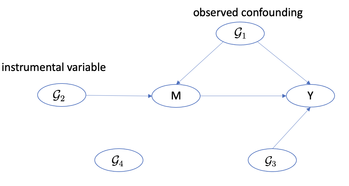
Figure 1: Diagram showing four different roles of the microbes in a microbiome-metabolome-disease pathway.

Estimation and inference of (1) and (2) have been discussed in the literature. In low-dimensional settings, $\boldsymbol{\beta}^{*}$, $\boldsymbol{\gamma}^{*}$, and $\theta^{*}$ can be estimated and tested using the ordinary least square (OLS). Due to the limited sample size and the large number of microbes in current multiview microbiome studies, high-dimensional methods are needed. For example, one can use regularized regression methods (e.g., Lasso) for parameter estimation and variable selection, and existing high-dimensional inference methods (e.g., the debiased Lasso (Zhang and Zhang,, 2014)) for constructing confidence intervals. In the ultrahigh-dimensional setting, Yu et al., (2022) further applies conditional variable screening to first filter out irrelevant predictors before performing penalized regression.

However, the validity of the above methods requires no hidden confounders. Specifically, if $\varepsilon_{i}$ in (1) is correlated with $\delta_{i}$ in (2), then there exist hidden confounders impacting the metabolite-disease link (e.g., diet, living habits). While traditional approaches like the two-stage least squares (2SLS, Angrist and Imbens,, 1995) method leverage instrumental variables that affect the outcome solely through the covariates of interest—e.g., single nucleotide polymorphisms (SNPs) in genetic studies (Lin et al.,, 2015)—the identification of suitable instrumental variables in microbiome research poses a challenge due to the complexity of microbial interactions and limited data availability. Nonetheless, the unknown group $\mathcal{G}_{2}$ implicitly delineates instrumental microbes. This revelation opens avenues for the development of a 2SLS-analogous approach tailored to circumvent hidden confounders within microbiome-metabolome-disease pathways, a prospect that will be further explored in the subsequent sections.

2.2 Integrative model for target and external microbiome studies

In this section, we address the hidden confounding issue by extending the target-only method to an integrative approach that leverages an external microbiome cohort. The main idea is to first predict the metabolite of interest using the external study and then infer the microbiome-metabolome-disease pathway based on the predicted values. Letting $\widetilde{m}_{j}$ and $\widetilde{\bf x}_{j}$ denote the metabolite of interest and the microbes in the external study, we consider

$$\widetilde{m}_{j}=\widetilde{\bf x}_{j}^{\intercal}\boldsymbol{\gamma}^{*}+\widetilde{\delta}_{j},$$ (3)

where each $\widetilde{\delta}_{j}$ follows a zero-mean normal distribution for $j=1,\ldots,N$. With an estimate of $\boldsymbol{\gamma}^{*}$ denoted by $\widehat{\boldsymbol{\gamma}}$ that will be discussed later, we predict $m_{i}$ in (1) with $\widehat{m}_{i}={\bf x}_{i}^{\intercal}\widehat{\boldsymbol{\gamma}}$ for $i=1,\ldots,n$. Then, we fit (1) with $m_{i}$ replaced by $\widehat{m}_{i}$:

$$y_{i}=\widehat{m}_{i}\theta+{\bf x}_{i}^{\intercal}\boldsymbol{\beta}+\xi_{i}\mbox{ for }i=1,\ldots,n.$$ (4)

This two-stage procedure boasts several advantages. Firstly, it enables the assessment of metabolites absent in the target cohort but present in the external cohort, a capability beyond the reach of the target-only method. This aspect is particularly pertinent given the frequent occurrence of missing metabolites in both targeted and untargeted metabolomics, as outlined in the Introduction. Secondly, the necessity for the external study to include the disease outcome is obviated, allowing for the utilization of data from a diverse array of sources. This feature significantly enhances the flexibility and broad applicability of our proposed integrative method.

We next study the theoretical property of this integrative method. First, since $\widehat{m}_{i}$ is a linear combination of ${\bf x}_{i}$, (4) may suffer from collinearity issues without additional constraints. To see what constraints are needed, we consider an oracle model where $\boldsymbol{\gamma}^{*}$ in (2) is known:

$$y_{i}={m}^{*}_{i}{\theta}^{*}+{\bf x}_{i}^{\intercal}\boldsymbol{\beta}^{*}+\epsilon_{i},$$ (5)

where $m^{*}_{i}={\bf x}_{i}^{\intercal}\boldsymbol{\gamma}^{*}$ and $\epsilon_{i}=\varepsilon_{i}+\theta^{*}\delta_{i}$ for $i=1,\ldots,n$. Based on the grouping of the microbes described in Section 2.1, we rewrite (5) as

$$y_{i}= ~{}\theta^{*}\left({\bf x}_{i}\right)_{\mathcal{G}_{1}}^{\intercal}\boldsymbol{\gamma}^{*}_{\mathcal{G}_{1}}+\theta^{*}\left({\bf x}_{i}\right)_{\mathcal{G}_{2}}^{\intercal}\boldsymbol{\gamma}^{*}_{\mathcal{G}_{2}}+\left({\bf x}_{i}\right)_{\mathcal{G}_{1}}^{\intercal}\boldsymbol{\beta}^{*}_{\mathcal{G}_{1}}+\left({\bf x}_{i}\right)_{\mathcal{G}_{3}}^{\intercal}\boldsymbol{\beta}^{*}_{\mathcal{G}_{3}}+\epsilon_{i}$$

$$= ~{}\left({\bf x}_{i}\right)_{\mathcal{G}_{1}}^{\intercal}\left(\theta^{*}\boldsymbol{\gamma}^{*}_{\mathcal{G}_{1}}+\boldsymbol{\beta}^{*}_{\mathcal{G}_{1}}\right)+\theta^{*}\left({\bf x}_{i}\right)_{\mathcal{G}_{2}}^{\intercal}\boldsymbol{\gamma}^{*}_{\mathcal{G}_{2}}+\left({\bf x}_{i}\right)_{\mathcal{G}_{3}}^{\intercal}\boldsymbol{\beta}^{*}_{\mathcal{G}_{3}}+\epsilon_{i}.$$ (6)

We observe that $\boldsymbol{\gamma}^{*}_{\mathcal{G}_{1}}$ and $\boldsymbol{\gamma}^{*}_{\mathcal{G}_{2}}$ are identifiable from (3). This, in turn, guarantees the identifiability of $\boldsymbol{\beta}^{*}_{\mathcal{G}_{1}}$ and $\theta^{*}$ in (2.2), if $\mathcal{G}_{2}\neq\emptyset$. This means that in practice, if $\widehat{\boldsymbol{\gamma}}$ has the same support as $\boldsymbol{\gamma}^{*}$ and $\mathcal{G}_{2}\neq\emptyset$, then the collinearity issue in (4) will likely be avoided.

The above observation highlights the importance of the following assumption that will be assumed true throughout the paper.

Assumption 1.

There exist microbes that are indirectly related to the outcome i.e., $\mathcal{G}_{2}\neq\emptyset$.

We next detail the estimation procedure. Specifically, we consider the following Lasso estimates based on (3) and (4):

$$\widehat{\boldsymbol{\gamma}}=\underset{\boldsymbol{\gamma}}{\text{argmin}}\biggl{\{}\sum_{j=1}^{N}\dfrac{(\widetilde{m}_{j}-\widetilde{\bf x}_{j}^{\intercal}\boldsymbol{\gamma})^{2}}{2N}+\lambda_{\gamma}\|\boldsymbol{\gamma}\|_{1}\biggr{\}},$$ (7)

and

$$\left(\widehat{\theta},\widehat{\boldsymbol{\beta}}\right)=\underset{\theta,\boldsymbol{\beta}}{\text{argmin}}\biggl{\{}\sum_{i=1}^{n}\dfrac{(y_{i}-\widehat{m}_{i}\theta-{\bf x}_{i}^{\intercal}\boldsymbol{\beta})^{2}}{2n}+\lambda_{\beta}\|\boldsymbol{\beta}\|_{1}\biggr{\}},$$ (8)

where $\lambda_{\gamma},\lambda_{\beta}>0$ are tuning parameters. In (8), we do not penalize $\theta$ because we do not want to shrink the effect of the host-metabolome interaction.

To study the theoretical properties of these Lasso estimates, we impose additional assumptions.

Assumption 2.

$(a)$ Each ${\bf x}_{i}$ i.i.d follows ansub-gaussian distribution.

$(b)$ Each $(\delta_{i},\varepsilon_{i})^{\intercal}$ i.i.d follows an zero-mean bivariate normal distribution.

$(c)$ There exists a constant ${\phi^{2}_{0\gamma}}$ such that

$$\frac{1}{N{\phi^{2}_{0\gamma}}}\|\widetilde{X}\Delta\|_{2}^{2}\geq\|\Delta_{S_{0}}\|_{2}^{2}$$

for all $\Delta\in\mathbb{R}^{p}$ satisfying $\|\Delta_{S_{0}^{c}}\|_{1}\leqslant 3\|\Delta_{S_{0}}\|_{1}$, where $S_{0}:=\{j:\gamma_{j}^{*}\neq 0\}$ and $\widetilde{X}=(\widetilde{\bf x}_{1},\ldots,\widetilde{\bf x}_{n})^{\intercal}$.

$(d)$ There exists a constant ${\phi^{2}_{0_{\beta}}}$ such that

$$\frac{1}{n\phi^{2}_{0_{\beta}}}\|X_{M}\Delta\|_{2}^{2}\geq\|\Delta_{S^{\prime}_{0}}\|_{2}^{2}$$

for all $\Delta\in\mathbb{R}^{p+1}$ satisfying $\|\Delta_{S_{0}^{{}^{\prime}c}}\|_{1}\leqslant 3\|\Delta_{S^{{}^{\prime}}_{0}}\|_{1}$, where $S^{\prime}_{0}:=\{j:\beta_{j}^{*}\neq 0\}$, and $X_{M}$ is an $n\times(p+1)$ matrix with the $i$-th row being $(m_{i}^{*},{\bf x}_{i})$ for $i=1,\ldots,n$.

Remark 1.

Assumption $2(a)$ is a common assumption about the design matrix $X$. Assumption $2(b)$ ensures that $\delta_{i}\theta^{*}+\varepsilon_{i}$ follows a normal distribution. Also, we do not require that $\delta$ is independent from $\varepsilon$, allowing for hidden confounders. Assumptions $2(c)$ and $2(d)$ are the restricted eigenvalue conditions (REC) for (3) and (2.2), respectively; see Bickel et al., (2009) for more discussions of REC.

The first result establishes the consistency of $\widehat{\boldsymbol{\gamma}},\widehat{\theta}$, and $\widehat{\boldsymbol{\beta}}$ defined in (7) and (8).

Proposition 1.

If Assumptions 1 and 2 hold, then

$$\|\widehat{\boldsymbol{\gamma}}-{\boldsymbol{\gamma}}^{*}\|_{1}=O(\lambda_{\gamma}s_{0_{\gamma}}),\;and\;|\theta^{*}-\widehat{\theta}|+\|\boldsymbol{\beta}^{*}-\widehat{\boldsymbol{\beta}}\|_{1}=O(\lambda_{\beta}(s_{0_{\beta}}+1))$$

for $\lambda_{\beta}\asymp(\lambda_{\gamma}s^{2}_{0_{\gamma}}\vee\sqrt{\log p/n})$ and $s_{0_{\gamma}}=o(1/\lambda_{\gamma})$, where $s_{0_{\gamma}}=\|\boldsymbol{\gamma}^{*}\|_{0}$, $s_{0_{\beta}}=\|\boldsymbol{\beta}^{*}\|_{0}$.

Proposition 1 indicates the consistency of $\widehat{\boldsymbol{\gamma}},\widehat{\theta}$, and $\widehat{\boldsymbol{\beta}}$. However, this result cannot uncover $\mathcal{G}_{1},\mathcal{G}_{2},\mathcal{G}_{3}$, and $\mathcal{G}_{4}$ or enable hypothesis testing for $\theta^{*}$. We address this concern in two steps. In this first step, we develop a thresholding procedure to allow for the identification of the microbes in $\mathcal{G}_{1},\mathcal{G}_{2},\mathcal{G}_{3}$, and $\mathcal{G}_{4}$.

Assumption 3.

min${}_{j\in{S_{0}}}$$|\boldsymbol{\gamma}^{*}_{j}|>8\lambda_{\gamma}s_{0_{\gamma}}/\phi^{2}_{0_{\gamma}}$, and min${}_{j\in{S^{\prime}_{0}}}$ $|\boldsymbol{\beta}^{*}_{j}|>8\lambda_{\beta}s_{0_{\beta}}/\phi^{2}_{0_{\beta}}$.

The next result establishes the variable-selection consistency for the support of $\boldsymbol{\beta}^{*}$ and $\boldsymbol{\gamma}^{*}$, which jointly determine $\mathcal{G}_{1},\mathcal{G}_{2},\mathcal{G}_{3}$, and $\mathcal{G}_{4}$.

Theorem 1.

If Assumptions 1, 2, and 3 hold, then the thresholded estimators $\widehat{\gamma}_{\textnormal{thres},j}=\widehat{\gamma}_{j}\mathbbm{1}(|\widehat{\gamma}_{j}|\geq C_{2})$ and $\widehat{\beta}_{\textnormal{thres},j}=\widehat{\beta}_{j}\mathbbm{1}(|\widehat{\beta}_{j}|\geq C^{\prime}_{2})$ with $C_{2}\geq 4\lambda_{\gamma}s_{0_{\gamma}}/\phi^{2}_{0_{\gamma}}$ and $C^{\prime}_{2}\geq 4\lambda_{\beta}s_{0_{\beta}}/\phi^{2}_{0_{\beta}}$ satisfy

$$P(\textnormal{sign}(\widehat{\boldsymbol{\gamma}}_{\textnormal{thres}})=\textnormal{sign}(\boldsymbol{\gamma}^{*}))\rightarrow 1\;and\;P(\textnormal{sign}(\widehat{\boldsymbol{\beta}}_{\textnormal{thres}})=\textnormal{sign}(\boldsymbol{\beta}^{*}))\rightarrow 1\;as\;N,n\rightarrow\infty,$$

where sign $(\cdot)$ is the sign function that maps positive entry to 1, negative entry to -1, and zero to zero.

In the second step, we aim to test ${\theta^{*}}=0$ by debiasing $\widehat{\theta}$ following the general idea in Zhang and Zhang, (2014). Specifically, let ${\bf z}=\widehat{{\bf m}}-X\widehat{{\bf b}}$, where

$$\widehat{{\bf b}}=\underset{{\bf b}}{\text{argmin}}\biggl{\{}\sum_{i=1}^{n}\dfrac{(\widehat{m}_{i}-{{\bf b}}^{\intercal}{\bf x}_{i})^{2}}{2n}+\lambda_{z}\|{\bf b}\|_{1}\biggr{\}}.$$ (9)

Our debiased Lasso estimator of $\theta^{*}$ is defined as

$$\widetilde{\theta}=\widehat{\theta}+\dfrac{{\bf z}^{\intercal}({{\bf y}}-\widehat{{\bf m}}\widehat{\theta}-X\widehat{\boldsymbol{\beta}})}{{\bf z}^{\intercal}\widehat{{\bf m}}},$$ (10)

where $\widehat{\theta}$ and $\widehat{\boldsymbol{\beta}}$ are given in (8).

Remark 2.

By the Karush–Kuhn–Tucker condition (KKT), we have

$$-X^{\intercal}(\widehat{{\bf m}}-X\widehat{{\bf b}})+\lambda_{z}{\bf s}=0\>\>\>\>\textnormal{for \> some}\>{\bf s}\in\partial\|\widehat{{\bf b}}\|_{1},$$

where $\partial\|\widehat{{\bf b}}\|_{1}$ is the subdifferential of the $l_{1}$ norm. Specifically, $s_{j}=\textnormal{sign}(\widehat{b}_{j})\text{ if}\>\>\>\widehat{b}_{j}\neq 0$ and $s_{j}\in[-1,1]\text{ if}\>\>\>\widehat{b}_{j}=0$ for $j=1,\ldots,p$. Therefore, when $\lambda_{z}\neq 0$, we know $\widehat{{\bf m}}-X\widehat{{\bf b}}\neq{\bf 0}$, or equivalently, ${\bf z}\neq{\bf 0}$.

Based on (10), we decompose $\widetilde{\theta}$ into three components: $\theta^{*}$, the noise (related to both $\boldsymbol{\varepsilon}$ and $\boldsymbol{\delta}$), and the bias:

$$\widetilde{\theta}=\theta^{*}+\underset{\textnormal{noise}}{\underbrace{\dfrac{{\bf z}^{\intercal}\boldsymbol{\varepsilon}}{{\bf z}^{\intercal}\widehat{{\bf m}}}+\dfrac{{\bf z}^{\intercal}\boldsymbol{\delta}\theta^{*}}{{\bf z}^{\intercal}\widehat{{\bf m}}}}}+\underset{\textnormal{bias}}{\underbrace{\sum_{k=1}^{p}\dfrac{{\bf z}^{\intercal}{\bf x}_{\cdot k}(\beta_{k}-\widehat{\beta}_{k})}{{\bf z}^{\intercal}\widehat{{\bf m}}}+\sum_{l=1}^{p}\dfrac{{\bf z}^{\intercal}{\bf x}_{\cdot l}(\gamma_{l}-\widehat{\gamma}_{l})\theta^{*}}{{\bf z}^{\intercal}\widehat{{\bf m}}}}},$$ (11)

where ${\bf x}_{\cdot k}$ represents the $k$-th column of $X$. Based on this decomposition, Theorem 2 below shows that $\widetilde{\theta}$ follows an asymptotic normal distribution.

Theorem 2.

Suppose Assumptions 1 and 2 hold. If $\underset{j}{\max}$ ${\bf z}^{\intercal}{\bf x}_{\cdot j}/\|{\bf z}\|_{2}=O_{p}(\sqrt{\log p})$, $\lambda_{\gamma}\asymp\sqrt{\log p/N}$, $\lambda_{\beta}\asymp(\lambda_{\gamma}s^{2}_{0_{\gamma}}\vee\sqrt{\log p/n})$, $s_{0_{\gamma}}=o_{p}(\sqrt{N/\log p})$, and $s_{0_{\beta}}=o(\sqrt{N}/(s^{2}_{0_{\gamma}}\log p)\wedge\sqrt{n}/\log p)$, then we have

$$\dfrac{{\bf z}^{\intercal}\widehat{{\bf m}}}{\|{\bf z}\|_{2}}(\widetilde{\theta}-\theta^{*})\xrightarrow{\text{d}}N(0,\sigma^{2}_{\theta^{*}})$$ (12)

as $N,n\rightarrow\infty$, where $\sigma^{2}_{\theta^{*}}={\sigma}^{2}_{\varepsilon}+{\theta^{*}}^{2}{\sigma}^{2}_{\delta}+2\theta^{*}\text{Cov}(\varepsilon_{i},\delta_{i}).$

If Cov($\varepsilon_{i},\delta_{i})=0$, i.e., no hidden confounders, then $\sigma^{2}_{\theta^{*}}={\sigma}^{2}_{\varepsilon}+{\theta^{*}}^{2}{\sigma}^{2}_{\delta}.$ In contrast, if Cov($\varepsilon_{i},\delta_{i})\neq 0$, then $\text{Cov}(\varepsilon_{i},\delta_{i})$ may not be estimated. Specifically, when the metabolite of interest is missing in the target cohort and the disease outcome is missing in the external cohort, $\text{Cov}(\varepsilon_{i},\delta_{i})$ is not estimable. Nonetheless, under $H_{0}:\theta^{*}=0$, $\sigma^{2}_{\theta^{*}}$ reduces to ${\sigma}^{2}_{\varepsilon}$, which can be estimated based on the target cohort. This enables the construction of an asymptotic $p$-value for testing $H_{0}$.

Corollary 1.

Suppose the assumptions in Theorem 2 hold. Under $H_{0}:\theta^{*}=0$, we have

$$\dfrac{{\bf z}^{\intercal}\widehat{{\bf m}}}{\|{\bf z}\|_{2}}\widetilde{\theta}\xrightarrow{\text{d}}N(0,\sigma^{2}_{\varepsilon})$$ (13)

as $N,n\rightarrow\infty$.

We use a robust estimator $\widehat{\sigma}^{2}_{\varepsilon}=\|{\bf y}-\widehat{{\bf m}}\widehat{\theta}-X\widehat{\boldsymbol{\beta}}_{\lambda_{\textnormal{cv}}}\|_{2}/(n-\|\widehat{\boldsymbol{\beta}}_{\lambda_{\textnormal{cv}}}\|_{0})$, where $\lambda_{\textnormal{cv}}$ is tuned by 10-fold cross-validation (Reid et al.,, 2016). The two-sided $p$-value is then defined as

$$p=2P(Z\geq|{\bf z}^{\intercal}\widehat{{\bf m}}\widetilde{\theta}|/(\|{\bf z}\|_{2}\widehat{\sigma}^{2}_{\varepsilon})),$$ (14)

where $Z$ follows the standard normal distribution.

As discussed in Section 2.1, the debiased inference may not yield a valid $p$-value for testing $H_{0}$ for the target-only method if hidden confounders exist (i.e., $\text{Cov}(\varepsilon_{i},\delta_{i})\neq 0$). In contrast, Corollary 1 suggests that by leveraging an external data set and using the two-stage procedure discussed above, an asymptotically valid $p$-value for testing $H_{0}$ is attainable by de-biasing. This further suggests that for target-only scenario, we can first randomly split this target dataset into two parts, one serving as the new target data, and the other serving as the external cohort. With this data splitting, we can apply the integrative framework to test $H_{0}$. While this sample-splitting method guarantees the validity of the inference, a potential issue is that the resulting $p$-value may depend on the specific data splitting. A possible solution is to repeat this data-splitting procedure multiple times to obtain multiple $p$-values. Then, an efficient $p$-value combination method, such as an extension of the rank-transformed subsampling method (Guo and Shah,, 2023), can be used to obtain a consensus $p$-value, which we leave for future investigation.

2.3 Causal implications

In this section, we discuss the potential causal implications of the proposed structural equation model. We consider a scenario with hidden confounders, where $\varepsilon_{i}$ in (1) and $\delta_{i}$ in (2) are correlated. Such hidden confounders have received increasing attention in the existing literature. For example, Guo et al., (2018) proposed a high-dimensional structural model to account for hidden confounders; here, we illustrate its univariate version adapted with our notation:

$$y_{i}=m_{i}\theta^{*}+\varepsilon_{i}$$ (15)

where $\varepsilon_{i}={\bf u}_{i}^{\intercal}\boldsymbol{\phi}_{1}+e_{i}$, and $m_{i}={\bf u}_{i}^{\intercal}\boldsymbol{\phi}_{2}+\xi_{i}$. Here, ${\bf u}_{i}$ represents the hidden confounding variables and ${\bf u}_{i}$, $e_{i}$, and $\xi_{i}$ are mutually independent. In this case, one can verify that $\mbox{Cov}(m_{i},\varepsilon_{i})=\boldsymbol{\phi}_{1}^{\intercal}\mbox{Cov}({\bf u}_{i})\boldsymbol{\phi}_{2}\neq 0$. Our structural equation model (1) and (2) extend their framework by introducing additional observed confounders ${\bf x}_{i}$ assumed independent from the hidden confounders ${\bf u}_{i}$:

$$y_{i}=m_{i}\theta^{*}+{\bf x}_{i}^{\intercal}\boldsymbol{\beta}^{*}+\varepsilon_{i}$$ (16)

and $$m_{i}={\bf x}_{i}^{\intercal}\boldsymbol{\gamma}^{*}+\delta_{i},$$ (17)

where $\varepsilon_{i}={\bf u}_{i}^{\intercal}\boldsymbol{\phi}_{1}+e_{i}$ and $\delta_{i}={\bf u}_{i}^{\intercal}\boldsymbol{\phi}_{2}+\xi_{i}$. Similarly, we have $\mbox{Cov}(\varepsilon_{i},\delta_{i})=\boldsymbol{\phi}_{1}^{\intercal}\mbox{Cov}({\bf u}_{i})\boldsymbol{\phi}_{2}\neq 0$. By accounting for both observed and hidden confounders, $\theta^{*}$ in (16) characterizes the causal effect of $m_{i}$ on $y_{i}$. Thus, since the proposed integrative procedure can efficiently account for hidden confounders, the $p$-value defined in (14) may be used to identify metabolites that causally impact the disease outcome.

2.4 Partially informative external dataset

All theoretical results established in Section 2.2 are based on a critical assumption: the target and external data share the same model for microbiome-metabolome interaction; that is, the same $\boldsymbol{\gamma}^{*}$. Unfortunately, this assumption may be violated and cannot be directly checked in practice when the metabolite of interest is missing in the target dataset. Therefore, we first take a theoretical approach to understand the potential impact of using a partially informative external data set.

Let the regression coefficient in the target and external data be ${\boldsymbol{\gamma}}^{*}$ and $\widetilde{\boldsymbol{\gamma}}^{*}$, respectively. We make the following assumption.

Assumption 4.

$\|\widetilde{\boldsymbol{\gamma}}^{*}-\boldsymbol{\gamma}^{*}\|_{1}\lesssim s_{0_{\boldsymbol{\gamma}^{\prime}}}\sqrt{\log p/N}$ with $s_{0_{\boldsymbol{\gamma}^{\prime}}}\lesssim s_{0_{\boldsymbol{\gamma}}}$, where $s_{0_{\gamma^{\prime}}}=\|\widetilde{\boldsymbol{\gamma}}^{*}\|_{0}$.

Assumption 5.

Assumption 2 (c) holds for $\widetilde{X}$ with respect to $\widetilde{S}_{0}:=\{j:\widetilde{\gamma}_{j}^{*}\neq 0\}$ with some constant ${\phi^{2}_{0_{\gamma^{\prime}}}}$, where $\widetilde{X}$ is given in Assumption 2 (c).

We have the following result.

Proposition 2.

Suppose Assumptions 1, 2, 4 and 5 hold. Let $\widehat{\boldsymbol{\gamma}^{\prime}}$ be estimated by equation (7) with a tuning parameter $\lambda_{\gamma^{\prime}}$. Denote $\widehat{\theta^{\prime}}$ and $\widehat{\boldsymbol{\beta}^{\prime}}$ as estimates from equation (8) with a tuning parameter $\lambda_{\beta^{\prime}}$. If $\lambda_{\gamma^{\prime}}\asymp\sqrt{\log p/N}$, we have

$$\|\widehat{\boldsymbol{\gamma}^{\prime}}-{\boldsymbol{\gamma}}^{*}\|_{1}=O(s_{0_{\gamma^{\prime}}}\sqrt{\log p/N}).$$

Furthermore, if $s_{0_{\gamma^{\prime}}}=o(\sqrt{N/\log p})$ and $\lambda_{\beta^{\prime}}\asymp(\lambda_{\gamma^{\prime}}s^{2}_{0_{\gamma^{\prime}}}\vee\sqrt{\log p/n})$, then

$$|\theta^{*}-\widehat{\theta^{\prime}}|+\|\boldsymbol{\beta}^{*}-\widehat{\boldsymbol{\beta}^{\prime}}\|_{1}=O(\lambda_{\beta^{\prime}}(s_{0_{\beta}}+1)).$$

In addition, if $s_{0_{\beta}}=o(\sqrt{N/(s^{4}_{0_{\gamma^{\prime}}}\log p)}\wedge\sqrt{n/\log p})$, we have

$$|\theta^{*}-\widehat{\theta^{\prime}}|+\|\boldsymbol{\beta}^{*}-\widehat{\boldsymbol{\beta}^{\prime}}\|_{1}\rightarrow 0.$$

Corollary 2.

Suppose the assumptions in Corollary 1 and Assumption 4 hold. Under $H_{0}:\theta^{*}=0$, we have

$$\dfrac{{\bf z}^{\intercal}\widehat{{\bf m}}}{\|{\bf z}\|_{2}}\widetilde{\theta}\xrightarrow{\text{d}}N(0,\sigma^{2}_{\varepsilon}),$$ (18)

where $\widehat{{\bf m}}$, ${\bf z}$ and $\widetilde{\theta}$ are obtained the same way as in Section 2.2.

In practice, Assumption 4 cannot be examined directly when the metabolite of interest is missing in the target data set. To ensure the informativeness of the external cohort, we should first guarantee that the target and external datasets focus on similar populations in terms of demographics and disease status. Furthermore, if the target study lacks the metabolite of interest, we may find an alternative metabolite that is highly correlated with the one of interest and observed in both studies. We then develop a data-driven method, called the “predictive correlation”, to examine the informativeness of the external cohort based on this highly correlated metabolite. Specifically, we first estimate $\boldsymbol{\gamma}^{*}$ and $\widetilde{\boldsymbol{\gamma}}^{*}$ from the target and external dataset, respectively. We then calculate $X\widehat{\boldsymbol{\gamma}}$ and $\widetilde{X}\widehat{\widetilde{\boldsymbol{\gamma}}}$ and calculate their correlation as an indicator of the informativeness of the external dataset, where a higher absolute correlation indicates higher informativeness. We will demonstrate the effectiveness of the proposed “predictive correlation” using numerical examples.

3 Simulation Study

3.1 Simulation with a fully informative external dataset

We conducted data-driven simulation studies to demonstrate the performance of the proposed estimation and inference procedures. The target microbiome dataset was obtained from an IBD study (Franzosa et al.,, 2019) (referred to as the FRAN study), where the relative abundances of 9973 bacterial genera for 220 subjects were collected. The external microbiome dataset was obtained from a colorectal cancer study, referred to as the YACHI study, which collected data for 347 subjects and 11317 bacterial genera (Yachida et al.,, 2019). To mitigate the potent impact of excess zeros in the microbial abundances, for both data sets, we filtered out microbes that were absent in more than 10% of the samples, resulting in 400 and 611 microbes for FRAN and YACHI, respectively. Among these microbes, 393 microbes were shared between FRAN and YACHI, which were our focus in this simulation. To account for the between-subject variation, for both datasets, we performed a centered log ratio (CLR, Aitchison,, 1982) transformation with a small value $10^{-8}$ added to the remaining zeros; the resulted data sets were denoted by $X$ and $\widetilde{X}$ for the target (FRAN) and external (YACHI) study, respectively.

The data generation procedure is detailed as follows. We first generated the metabolite of interest for the target data according to ${\bf m}=X\boldsymbol{\gamma}^{*}+\boldsymbol{\delta}$, where

$$\boldsymbol{\gamma}^{*}=(\underset{\textnormal{20}}{\underbrace{-0.5,...,-0.5}},0,...,0,\underset{\textnormal{20}}{\underbrace{0.5,...,0.5}})^{\intercal}.$$

With ${\bf m}$, we simulated the outcome ${\bf y}$ according to ${\bf y}={\bf m}\theta^{*}+X\boldsymbol{\beta}^{*}+\boldsymbol{\varepsilon}$, where

$$\boldsymbol{\beta}^{*}=(\underset{\textnormal{10}}{\underbrace{0.1,...,0.1}},\underset{\textnormal{30}}{\underbrace{-0.1,...,-0.1}},0,...,0)^{\intercal},$$

and $\theta^{*}$ will be set to various values to examine the effectiveness of the proposed method in detecting various levels of metabolite-disease associations. The error terms $\boldsymbol{\delta}$ in the metabolite and $\boldsymbol{\varepsilon}$ were drawn from a bivariate normal distribution with mean zero and a covariance matrix of $\rho$ for off-diagonal entries and 1 for diagonal entries. When $\rho\neq 0$, $\boldsymbol{\delta}$ and $\boldsymbol{\varepsilon}$ are correlated due to the existence of latent variables that confound the metabolite-disease association. The external metabolite $\widetilde{{\bf m}}$ was generated according to $\widetilde{\bf m}=X\boldsymbol{\gamma}^{*}+\boldsymbol{\delta}$, where entries of $\widetilde{\boldsymbol{\delta}}$ were independently generated independently from a standard normal distribution. The same $\boldsymbol{\gamma}^{*}$ was used to generate ${\bf m}$ and $\widetilde{\bf m}$, representing an ideal scenario where the external data set is fully informative of the target data. Under this data-generation regime, we can elucidate the roles of the 393 microbes according to the non-zero entries of $\boldsymbol{\beta}^{*}$ and $\boldsymbol{\gamma}^{*}$. Specifically, 20 microbes belong to $\mathcal{G}_{1}$, acting as confounders; 20 microbes belong to $\mathcal{G}_{2}$, playing an instrumental role. 20 microbes that belong to $\mathcal{G}_{3}$ are directly predictive of the disease outcome; the remaining 333 microbes are irrelevant.

We first examined the effect of the external sample size on the estimation and inference accuracy of $\theta^{*}$. Specifically, we sub-sampled $m$ individuals from the full external data $\{\widetilde{X},\widetilde{\bf m}\}$ without replacement with $N=150,200,300$, while using all individuals in the target data ($n=220$). We considered $\rho=0$ and $0.25$, representing cases with/without hidden confounders, respectively. For estimation, we set $\theta^{*}=0.2$ and examined the estimation bias. For inference, we considered $\theta^{*}=0,0.1,0.12,0.14,0.16,0.18,0.2$. The type-I error rate and power were evaluated for $\theta^{*}=0$ and $\theta^{*}\neq 0$, respectively.

We compared the proposed integrative method in Section 2.2 to the target-only method in Section 2.1. Note that, in practice, the target-only analysis is not attainable when the metabolite of interest is not collected in the target data. All tuning parameters in both methods were selected using 5-fold cross-validation. The estimation bias, type-I error rate, and power were examined based on 100 replications.

Figure 2(a) and 2(b) show the estimation bias of both methods with the external sample size $N=150,200,250$ for $\rho=0$ and $0.25$, respectively. Since the target-only method does not involve the external data, its performance does not vary with external sample size. The target-only method appears slightly more accurate than the proposed muti-view method when $\rho=0$ (Fig. 2(a)). This is because in this case, no hidden confounders exist, and the target-only method is guaranteed to yield consistent estimation of $\theta^{*}$. On the other hand, despite using a fully informative external data set, the integrative method could still suffer from the prediction error arising from the randomness in the external data. However, when $\rho=0.25$, the target-only method shows a systematic bias, whereas the integrative method yields less bias when the external size increases (Fig. 2(b)). The systematic bias comes from the hidden confounding effect characterized by $\rho$. Indeed, when $\rho$ increases, i.e., the confounding effect becomes stronger, we anticipate a heavier estimation bias for the target-only method.

Similar to the estimation accuracy, when $\rho=0$, the target-only method outperforms the integrative method in terms of power, while both methods can control the type-I error rate (Fig. 2(c)). Nonetheless, Fig. 2(d) shows that when $\rho=0.25$, the target-only method suffers from a highly inflated type-I error rate. In contrast, our integrative method has a well-controlled type-I error rate and decent power.

(a)

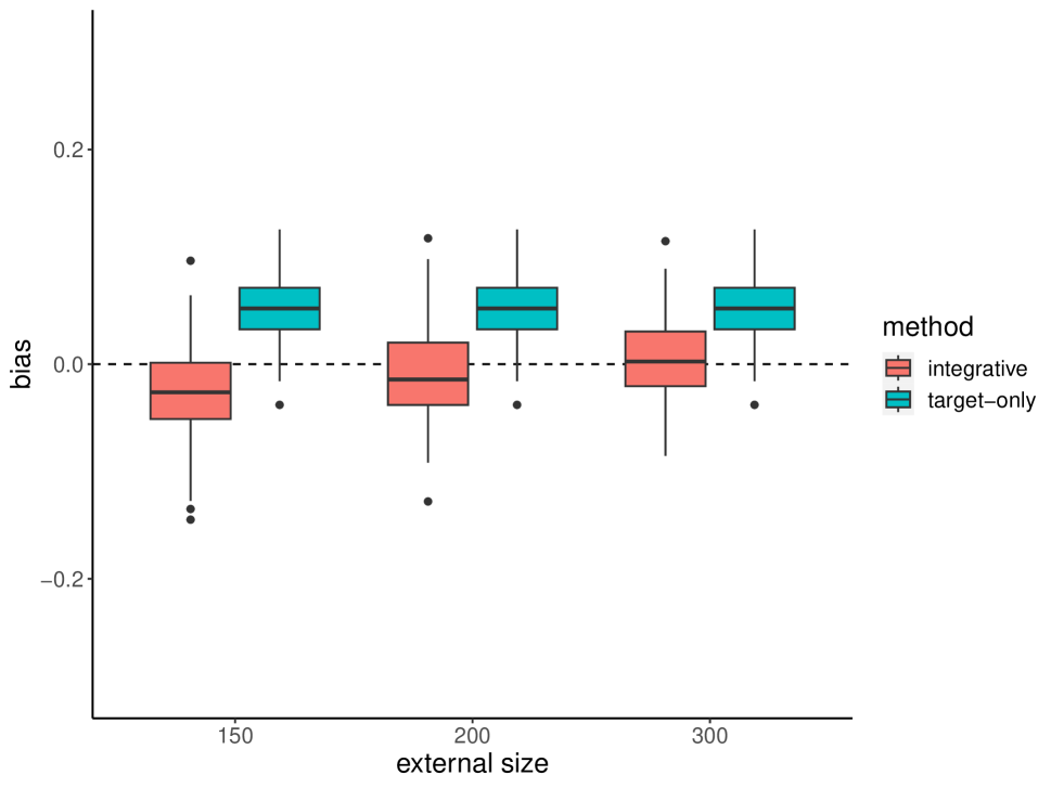
(b)

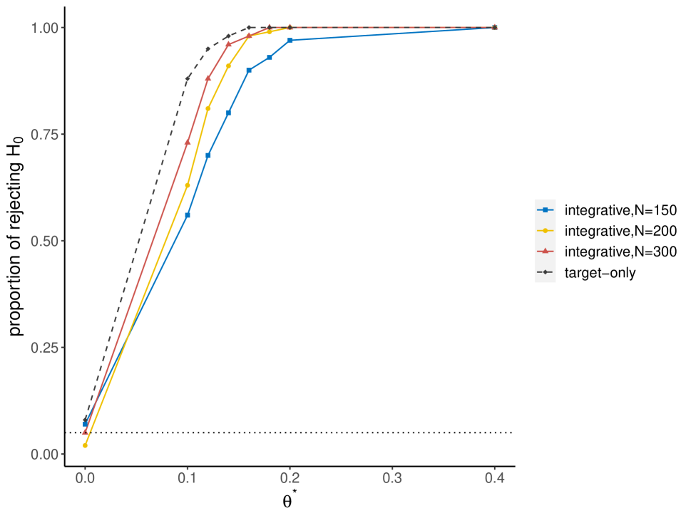
(c)

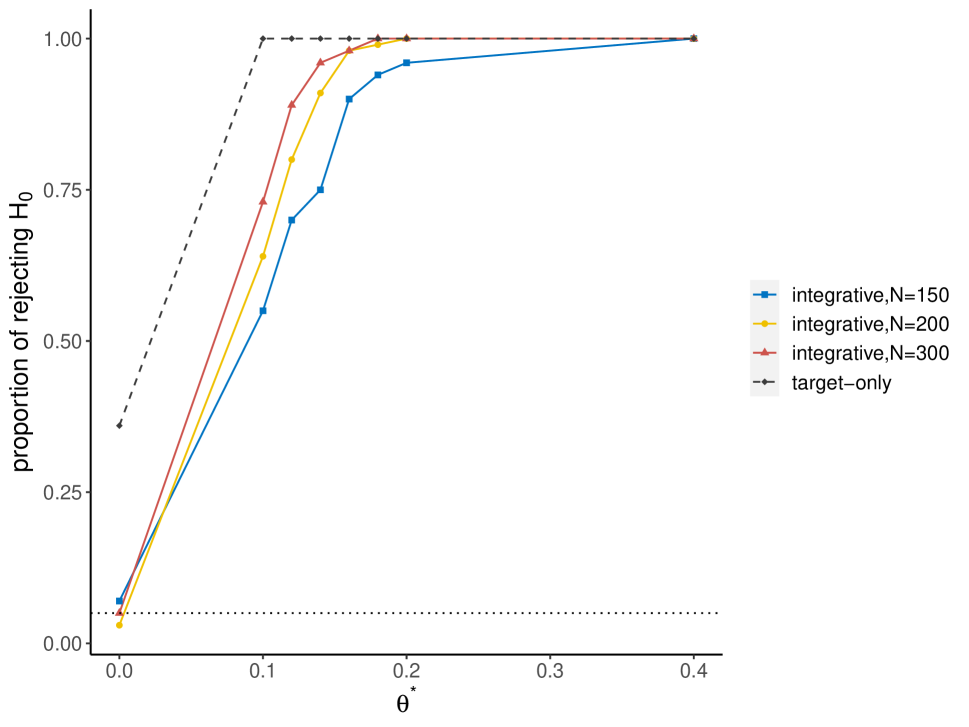
(d)

Figure 2: The boxplot of the bias $\tilde{\theta}-\theta^{*}$ with $\theta^{*}=0.2$ for integrative method and target-only method under different external sample size ($\rho=0$ in (a) and $\rho=0.25$ in (b)). The lineplot of the type-I error and power for the integrative method and target-only method under different external sample sizes ($\rho=0$ in (c) and $\rho=0.25$ in (d)), and the horizontal dotted line represents a value of 0.05.

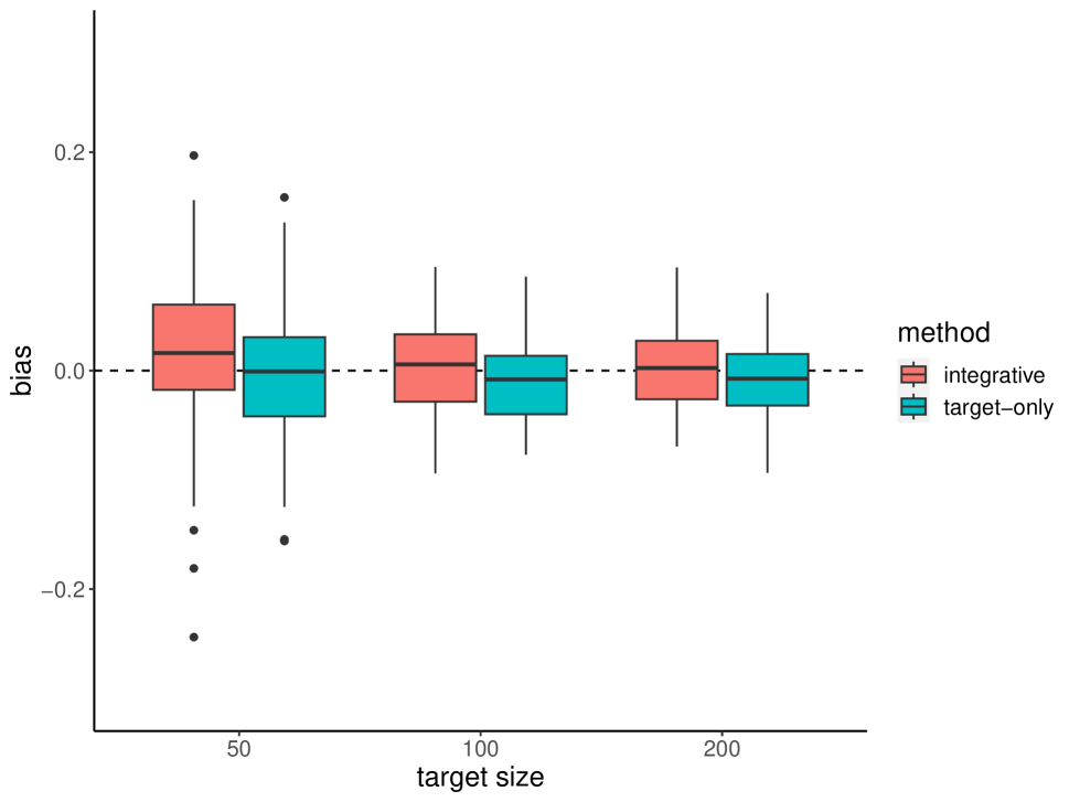
(a)

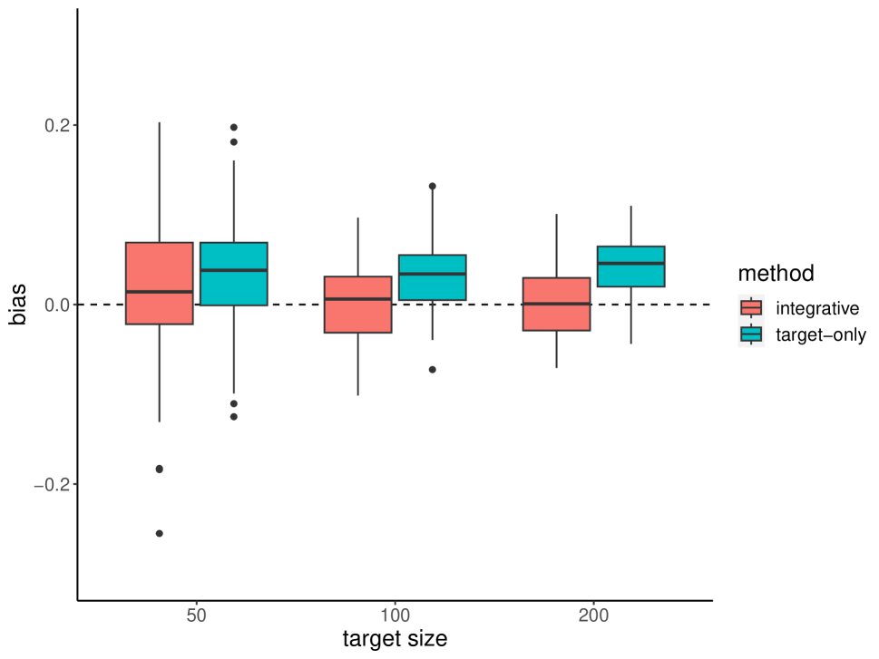
(b)

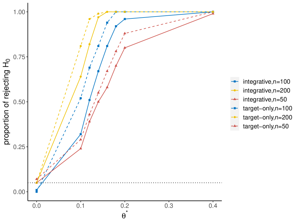
(c)

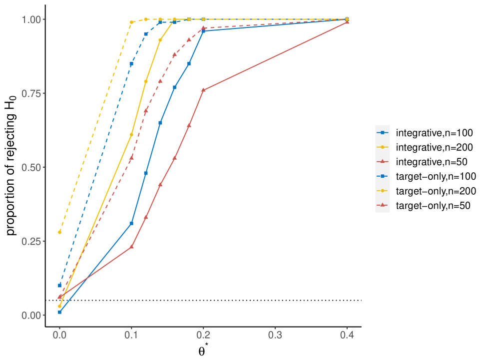
(d)

Figure 3: The boxplot of the bias $\tilde{\theta}-\theta^{*}$ with $\theta^{*}=0.2$ for integrative method and target-only method under different target sample size ($\rho=0$ in (a) and $\rho=0.25$ in (b)). The lineplot of the type-I error and power for the integrative method and target-only method under different target sample sizes ($\rho=0$ in (c) and $\rho=0.25$ in (d)), and the horizontal dotted line represents a value of 0.05.

We also studied the impact of the target sample size for estimating and inferring $\theta^{*}$. We sub-sampled $n$ individuals from the full target data $\{X,{\bf m},{\bf y}\}$ without replacement, where $n=50,100,200$. We used the full external data of 347 individuals. In this case, both the target-only and the integrative method are impacted by different values of $n$. Figure 3(a) shows that the integrative and target-only methods have a similar performance when $\rho=0$, while Figure 3(b) suggests a systematic bias for the target-only method when $\rho=0.25$, which is also observed in Fig. 2(b). When $\rho=0$, that is, no latent confounders, the target-only method has a better performance compared to the integrative method, represented by a higher power and well-controlled type I error for each target sample size $n$ (Fig. 3(c)). Nonetheless, Fig. 3(d) shows that when $\rho=0.25$, the target-only method has a highly inflated type-I error rate. Notably, the type-I error rate of the target-only method increases with the target sample size because of the growing asymptotic bias. In contrast, the integrative method can still control the type-I error rate with decent power.

In conclusion, the target-only method works well when no latent confounders exist; however, its performance is highly sensitive to hidden confounding. In contrast, our integrative method shows robustness regarding the strength of latent confounding effects. Thus, our integrative method may benefit practitioners in real microbiome data analysis where latent confounders commonly exist.

3.2 Simulation for variable selection consistency

We demonstrate the performance of the proposed integrative method in terms of correct identification of the microbes in $\mathcal{G}_{j}$ for $j=1,\ldots,4$, the definition of which can be found in Section 2.1. Since each $\mathcal{G}_{j}$ is uniquely determined by the support of $\boldsymbol{\beta}^{*}$ and $\boldsymbol{\gamma}^{*}$, in this simulation, we evaluate the effectiveness of the proposed method in terms of estimating the support of $\boldsymbol{\beta}^{*}$ and $\boldsymbol{\gamma}^{*}$.

We consider the same simulation design as in Section 3.1 with $\rho=0.25$ except for an increased signal in $\boldsymbol{\beta}^{*}$ to facilitate the support detection; the new $\boldsymbol{\beta}^{*}$ is defined as

$$\boldsymbol{\beta}^{*}=(\underset{\textnormal{40}}{\underbrace{0.5,...,0.5}},0,...,0)^{\intercal}.$$

As discussed in Theorem 1, our procedure can lead to consistent variable selection with an additional thresholding step. In this simulation, the threshold was set as 0.1. Given $\widehat{\boldsymbol{\beta}}$, we calculated the true positive rate (TPR) and false positive rate (FPR) according to

$$\mbox{TPR}(\boldsymbol{\beta}^{*})=\frac{\sum_{j=1}^{p}\mathbbm{1}(\beta_{j}^{*}\neq 0\mbox{ and }\widehat{\beta}_{j}\neq 0)}{\sum_{j=1}^{p}\mathbbm{1}({\beta}^{*}_{j}\neq 0)},\mbox{FPR}(\boldsymbol{\beta}^{*})=\frac{\sum_{j=1}^{p}\mathbbm{1}(\beta_{j}^{*}=0\mbox{ and }\widehat{\beta}_{j}\neq 0)}{\sum_{j=1}^{p}\mathbbm{1}({\beta}_{j}^{*}=0)},$$

where $p=393$, and $\mbox{TPR}(\boldsymbol{\gamma}^{*})$ and $\mbox{FPR}(\boldsymbol{\gamma}^{*})$ can be defined in the same way. Similar to Section 3.1, we considered varying the sample size of the target and the external data by sub-sampling. For all scenarios, we plotted the TPRs and FPRs over 100 replications. Figure 4(a) shows that, as the external sample size increases, our integrative method leads to improved $\mbox{FPR}(\boldsymbol{\gamma}^{*})$ and $\mbox{TPR}(\boldsymbol{\gamma}^{*})$. Since the target sample size remains the same, $\mbox{FPR}(\boldsymbol{\beta}^{*})$ and $\mbox{TPR}(\boldsymbol{\beta}^{*})$ stay roughly unchanged. Fig. 4(b) shows that $\mbox{FPR}(\boldsymbol{\beta}^{*})$ and $\mbox{TPR}(\boldsymbol{\beta}^{*})$ improve with an increasing target size, while $\mbox{FPR}(\boldsymbol{\gamma}^{*})$ and $\mbox{TPR}(\boldsymbol{\gamma}^{*})$ remain nearly constant. Therefore, Fig. 4 demonstrates the effectiveness of the proposed thresholding procedure for recovering $\mathcal{G}_{j}$ for $j=1,\ldots,4$.

3.3 Simulation with a partially informative external study

In previous simulations, we have assumed the external dataset to be fully informative, which is, however, not guaranteed in practice. Thus, in this section, we study the impact of having a partially informative external dataset. Recall from Section 3.1 that $X$ and $\widetilde{X}$, respectively, denote the microbiome data matrix in the target (FRAN) and external (YACHI) study. The target metabolite ${\bf m}$ and disease outcome ${\bf y}$ were generated in the same way as in Section 3.1 except for some adjustment to the parameters; that is, $\theta^{*}=0$ or 0.3,

$$\boldsymbol{\gamma}^{*}=(\underset{\textnormal{5}}{\underbrace{0.025,...,0.025}},0,...,0,\underset{\textnormal{20}}{\underbrace{0.25,...,0.25}})^{\intercal},$$

and

$$\boldsymbol{\beta}^{*}=(\underset{\textnormal{40}}{\underbrace{0.1,...,0.1}},0,...,0)^{\intercal}.$$

We generated the external metabolite $\widetilde{\bf m}$ according to $\widetilde{\bf m}=X\widetilde{\boldsymbol{\gamma}}^{*}+\boldsymbol{\delta}$; here, $\widetilde{\boldsymbol{\gamma}}^{*}=\boldsymbol{\gamma}^{*}+{\bf e}$, where ${\bf e}\neq 0$ represents a partially informative external study. We considered two cases for ${\bf e}$. The first case represents a scenario of “scale change”, where $e_{l}$ is randomly draw from $\{-\tau/10,\tau/10\}$ for $l=1,2,...,5$ or $l=388,389,...,393$, and $e_{l}=0$ elsewhere. The second case represents a scenario of “position change”, where $e_{l}$ is randomly draw from $\{-\tau/10,\tau/10\}$ for $l=6,...,15$ and $e_{l}=0$ elsewhere. Let $\tau=\|\boldsymbol{\gamma}^{*}-\widetilde{\boldsymbol{\gamma}}^{*}\|_{1}$ represent the overall difference between $\boldsymbol{\gamma}^{*}$ and $\widetilde{\boldsymbol{\gamma}}^{*}$, with a smaller $\tau$ indicating more informativeness. We examined the type-I error rate when $\theta^{*}=0$ and the power when $\theta^{*}=0.3$ with varying values of $\tau=0.25,0.5,0.75,1,1.25,2,4$ at a two-sided significance level $\alpha=0.05$. We also used the ”predictive correlation” proposed in Section 2.4 as an alternative way to measure the informativeness of the external dataset. We used the entire target and external dataset in this simulation, and the type-I error rate and power were calculated over 100 replications.

Figure 5(a) shows that in both cases, the type-I error rate inflates and power decreases as $\tau$ increases. When the change is sufficiently small, e.g., when $\tau\leq 1$, the type-I error rate remains approximately controlled and power stays decent, which aligns with the theoretical result in Corollary 2. However, when $\tau$ is large, the external dataset becomes not informative, and the proposed method is unreliable indicated by either high type I error or low power. Therefore, these results emphasize the importance of choosing a proper external dataset. Figure 5(b) demonstrates that the proposed “predictive correlation” can help examine the informativeness of external datasets for the metabolite of interest. Specifically, when $\tau<1$, the “predictive correlation” remains around 0.8, whereas it shows a substantial drop as $\tau$ exceeds 1. These observations completely agree with the patterns of the type-I error rate and power in Figure 5(a). We will further demonstrate the use of the ”predictive correlation” in Section 4.

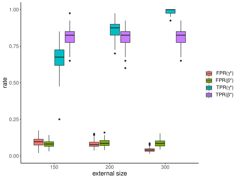
(a)

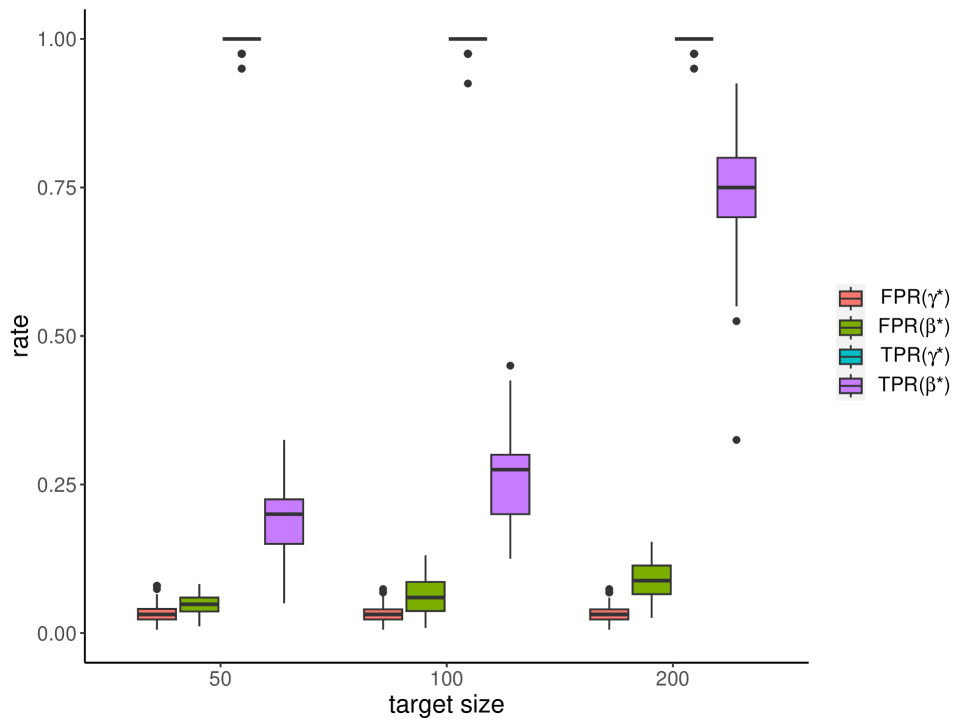
(b)

Figure 4: The true positive rate (TPR) and false positive rate (FPR) for $\boldsymbol{\beta}^{*}$ and $\boldsymbol{\gamma}^{*}$ with different external sample sizes (a) and target sample sizes (b).

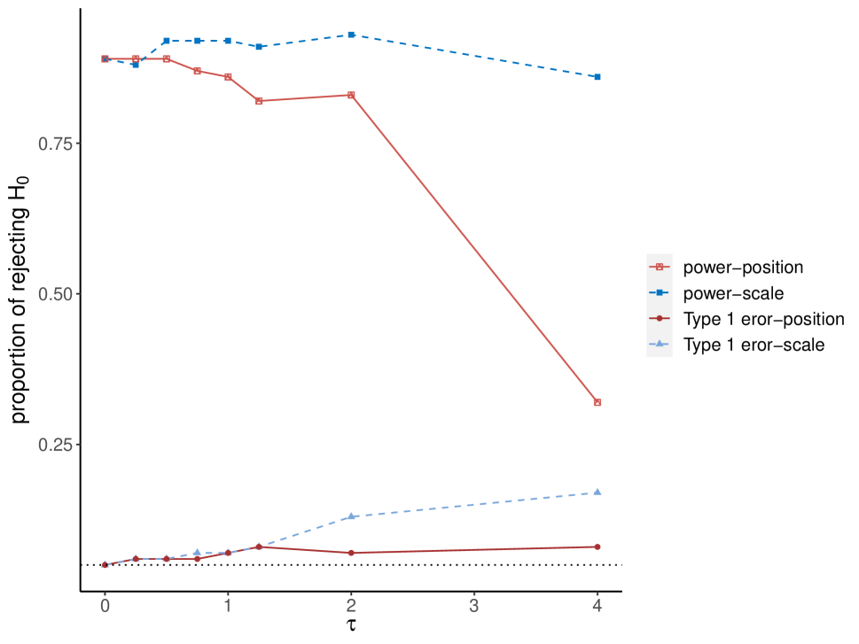
(a)

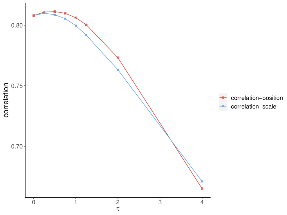
(b)

Figure 5: The line plot for the type-I error and power ($\theta^{*}=0.3$) for the integrative method under scale change (dashed) and position change (solid) in (a), along with the horizontal dotted line represent a value of 0.05. The corresponding line plot of the average correlation between predicted and fitted metabolites in (b).

4 Real Data Application

In this section, we aim to elucidate essential microbiome-metabolome interactions related to the disease pathology of IBD by integrating iHMP (target) and FRAN (external), respectively, described in Section 1 and 3.1.

4.1 Data collection and preprocessing

We considered 132 individuals from the iHMP cohort, who were initially screened for IBD symptoms with positive imaging as evidenced by colonic wall thickening or ileal inflammation or other symptoms related to chronic diarrhea or rectal bleeding. A total of 1,785 stool samples, which were collected every two weeks for each individual (with some dropout) using a home shipment protocol for one year. Metagenomic data were generated by shotgun sequencing of the DNA samples from 1,638 stool samples. For the metagenomic data, the raw fastq files were applied quality filtering, adapter trimming, and deduplication. If paired-end reads could not be merged, forward and reverse reads were concatenated into a single fastq file. The host DNA was filtered out using bowtie v2.3.5 (Langmead and Salzberg,, 2012), aligning reads to the human reference genome named Genome Reference Consortium Human Build 38. Next, Kraken v2.1.1 (Wood et al.,, 2019) and Bracken v2.8 (Lu et al.,, 2017) were run for taxonomic classification and species abundance estimation. Samples with less than 50,000 reads were discarded. Instead of the default reference database, a recently published version of GTDB (v207) is used for kraken (Youngblut and Ley,, 2021). Four LC–MS methods were used to profile metabolites from 546 stool samples, where two of them measured polar metabolites, one method measured metabolites of intermediate polarity (for example, fatty acids and bile acids), and a method tailored to lipid profiling. As discussed in Section 1, the primary IBD ourcome is CRP, measured from blood samples taken at the quarterly clinical visits.

The FRAN cohort consists of 226 individuals with 161 adult patients in Massachusetts General Hospital and 65 patients enrolled in two distinct studies from the Netherlands. The same protocol as in the iHMP study was used to collect and preprocess the metagenomic and metabolomic data. Unlike the iHMP cohort, the FRAN study only collected stool samples at baseline and measured no IBD-related biomarkers. Thus, despite FRAN’s larger sample size, we chose iHMP as our target data of discovery, while using FRAN as the external data to boost statistical power and biological relevance.

4.2 Preliminary analysis

Given the longitudinal architecture of the Integrated Human Microbiome Project (iHMP) dataset, our initial step involved selecting a singular measurement per participant for subsequent analysis. Specifically, we filtered for non-missing C-reactive protein (CRP) measurements, noting their corresponding visit dates. Measurements preceding any metagenomic and metabolomic profiling were excluded. We then identified the metagenomic and metabolomic dataset pairs immediately preceding each remaining CRP measurement. This process culminated in the selection of the earliest complete set of CRP, metagenomic, and metabolomic measurements for each individual. Consequently, our refined dataset comprised 40 subjects with no missing data across microbiome, metabolome, CRP levels, and other clinical covariates of interest, including 39 diagnosed with inflammatory bowel disease (IBD) and one healthy control. The resulting microbiome data set contained 7235 bacterial genera, which were further aggregated into 835 bacterial orders. More than 88% of data entries were zero. To mitigate the impact of the excess zeros, we removed microbes that were absent in more than 30% of the individuals; as a result, 63 microbial orders remained. This additional filtering step also helped address the issue of having a relatively small sample size ($n=40$). To account for the compositional nature of the microbiome data, we added a small number $10^{-8}$ to each data entry, followed by the CLR transformation. We then performed quality control for the metabolites based on their annotation, measure confidence, and missing data. Specifically, among the total of 81,868 metabolites, we only included metabolites that had corresponding HMDB IDs, were measured with high confidence, and had no missing data. As a result, 143 metabolites remained. We further accounted for their skewness by taking the log transformation for each of the remaining metabolite measurements, followed by standardization. Similar to Section 1, by MiRKAT, we found 87 (61%) metabolites significantly associated with the microbes, indicating strong microbiome-metabolome interactions despite a relatively small sample size. We also performed a correlation test for age and a two-sample t-test for gender in the iHMP cohort, but no significance was found with $p$-values of 0.315 and 0.19, respectively. Thus, we would not include them in downstream analyses due to our small sample size. However, our integrative framework can be easily extended to include observed confounders and is robust to hidden confounders.

Similar analyses were performed for the FRAN dataset. Specifically, the original microbiome data consisted of 9973 bacterial genera, which were aggregated into 1282 bacterial orders. After removing orders absent in more than 30% of the individuals, 104 orders remained; among them, 61 orders were also measured in the iHMP data set, which were the focus of the integrative analyses detailed in Section 4.4. Only 47 metabolites were confidently measured with corresponding HMDB IDs and no missing values, which were further log-transformed and standardized for downstream analysis. Among them, 23 were also detected in the iHMP dataset, while the rest 24 were uniquely identified in the FRAN dataset. Such an issue of limited overlapping metabolites between studies is common for untargeted metabolomics studies, hindering comprehensive biological findings. As highlighted in Section 2.2, our proposed integrative approach has the strength to examine the association of CRP (only available in iHMP) and those 24 metabolites that were unique to FRAN; see Section 4.4 for details.

4.3 Target-only analysis of the iHMP data

In this section, we solely rely on the iHMP cohort and fitted the target-only method in Section 2.1 to detect metabolites that were microbially regulated and significantly associated with CRP. We focused on the 87 significant metabolites identified by MiRKAT in Section 4.2 and the 61 bacterial orders that were shared between the iHMP and FRAN cohort. The target-only method was applied for each metabolite separately, and we generated a volcano plot showing the estimated coefficient and the corresponding $p$-value for each metabolite (Figure 6 (a)). After accounting for the direct effect of microbes, five metabolites were significantly associated with CRP under a two-sided significance level 0.05. Notably, they all have negative effects on CRP, meaning that they may play an anti-inflammatory role. Specifically, they are maslinic acid, 4-hydroxybenzaldehyde, lysope, alpha-linolenic acid, and taurocholic acid. Maslinic acid has exerted potent anti-inflammatory action by inhibiting the production of Nitric Oxide and tumor necrosis factor alpha (Huang et al.,, 2011). It has been reported that the 4-hydroxybenzaldehyde protects against DSS-induced colitis by regulating immune tolerance and excessive inflammatory responses (Shin et al.,, 2018). Lysope is a minor component of the cell membrane (Makide et al.,, 2009) and it also functions as a neuronutrient activator through the mitogen-activated protein kinase signaling pathway in pheochromocytoma cells (Nishina et al.,, 2006). Alpha-linolenic acid supplementation was shown to be effective in inhibiting inflammation induced by IL-1$\beta$ by down-regulating mRNA levels of pro-inflammatory genes including IL-8, COX2 and inducible nitric oxide synthase (Reifen et al.,, 2015). Lastly, the taurocholic acid could promote the promotes pathobiont and colitis in the mice study (Devkota et al.,, 2012). However, we acknowledge two potential limitations of this iHMP-only analysis. First, we may have compromised statistical power due to the limited sample size of 40, despite the strong signal of microbiome-metabolome interactions detected in Section 4.2. Second, as illustrated in Section 3, the target-only method is sensitive to hidden confounders, leading to inflated type-I error rates. While the second limitation may be addressed by sample-splitting (see at the end of Section 2.2 for details), a lack of statistical power can be foreseen given the small total sample size. Therefore, we will address these two limitations by applying the integrative method proposed in Section 2.2 to an informative external cohort (FRAN).

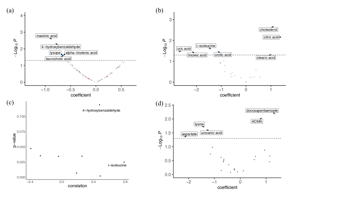
Figure 6: The volcano plot of the coefficient vs. $p$-value (in -log₁₀) of each metabolite using target-only method (from iHMP dataset in (a)) and integrative method (overlapping metabolites in (b) and unique metabolites from FRAN dataset in (d)). The horizontal dashed line represents the $p$-value threshold of 0.05. The blue dots represent the significant metabolites. The red dots in (a) denote the metabolites that are significant in (b). The red dot in (b) denotes the metabolite (4-hydroxybenzaldehyde) that is significant in (a). The scatter plot of the predictive correlation vs. $p$-value for the overlapping metabolites is in (c).

4.4 Integration of iHMP and FRAN data

In this section, we aim to improve the statistical power and biological relevance of the target-only analysis performed in Section 4.3. Specifically, we focused on the 47 microbially-regulated metabolites in the FRNA cohort and applied the proposed intergrative method to each of them separately. Figure 6 (b) shows the estimated coefficients and corresponding $p$-values obtained from the integrative method for the 23 overlapping metabolites. We identified 8 metabolites (colored in red) that showed different results between Figs. 6 (a) and (b). Specifically, 7 metabolites that are insignificant in Fig. 6 (a) become significant in Fig. 6 (b), while one metabolite is significant in Fig. 6 (a) but becomes insignificant in Fig. 6 (b). To further understand these discrepencies, we calculated the “predictive correlations” for these 8 metabolites, which were further plotted against their corresponding $p$-values in Fig. 6 (c), where the $p$-values were obtained from the integrative analysis. All metabolites except for I-isoleucine had low “predictive correlations”, suggesting that the inconsistent results could be due to the low informativeness of the FRAN cohort regarding these metabolites. However, the “predictive correlation” of I-isoleucine is close to 0.8, which may suggest that I-isoleucine is indeed involved in the microbiome-CRP pathway, while the insignificant $p$-value in Fig. 6 (a) is due to a lack of statistical power. These “predictive correlation” results also indicate that any external cohort may be informative regarding a subset of metabolites but not for all of them.

As discussed earlier, an important merit of the proposed integrative method is its capability of analyzing metabolites that are missing in the target cohort yet observed in the external cohort. Figure 6 (d) identified 5 significant metabolites that were only observed in the FRAN cohort: asymmetric dimethylarginine (ADMA), lysine, urocanic acid, aspartate, and docosapentaenoate (DPA). All of them have been widely discussed in the existing literature as IBD-related metabolites. Specifically, ADMA is an endogenous inhibitor of nitric oxide (NO) synthase, which is a mediator of immunity and inflammation related to IBD (Sahin et al.,, 2006). The disturbance in lysine could have relevant consequences in IBD prognosis (Aldars-Garcia et al.,, 2021). The urocanic acid demonstrates its anti-inflammatory ability in IBD by incubating with biopsies to produce lower levels of proinflammatory cytokines (Kammeyer et al.,, 2012). The DPA also shows anti-inflammatory properties via regulation of the production of inflammatory cytokines and the pathway of eicosanoid synthesis (Zheng et al.,, 2019).

Our integrative framework can also characterize the roles that individual microbes play in the detected pathways. For example, Table 1 categorizes individual microbes into $\mathcal{G}_{j}$ for $j=1,\ldots,3$ to elucidate their roles in the DPA-CRP pathway; $\mathcal{G}_{4}$ was ommitted from the table from it includes irrelavant microbes. One microbe was detected to directly impact both DPA and CRP; 6 microbes play instrumental roles that affect CRP only through DPA; 5 microbes directly affect CRP without involving DPA. Among the six instrumental microbes, Erysipelotrichales has a decreased abundance in IBD patients compared to healthy controls (Kaakoush,, 2015). Thus, our result provides an explanation for the Erysipelotrichales-IBD link that Erysipelotrichales may affect IBD through the synthetic process of metabolite DPA.

Groups	Microbes
$\mathcal{G}_{1}$	UMGS1883
$\mathcal{G}_{2}$	Erysipelotrichales, Tissierellales, Christensenellales, Saccharofermentanales, Sphingobacteriales, and UBA1212
$\mathcal{G}_{3}$	Peptostreptococcales, Bacillales_B, Deinococcales, Chitinophagales and Propionibacteriales

Table 1: Summary of roles of Microbes that related to DPA to the pathway of CRP level

5 Discussion

This paper first proposes a target-only method to integrate microbiome, metabolites, and disease outcomes to identify relevant microbiome-metabolome-disease pathways. However, this method may have compromised statistical power and be sensitive to hidden confounders. We then address these issues by proposing an integrative framework that leverages an informative external data set. The effectiveness of the integrative method is demonstrated using multiple simulation studies even when the external data set is not fully informative. A data-driven procedure is also provided to examine the informativeness of the data set. Compared to the target-only method, an additional benefit of the integrative method is that it can analyze metabolites missing in the target data. This is demonstrated through the real data application, yielding biologically meaningful microbiome-metabolome-IBD pathways despite a relatively small sample size.

The proposed framework can be easily extended to include observed covariates due to the flexibility of $l$-1 penalized models. In practice, there may be multiple external cohorts which are all partially informative to the target. In this case, instead of using only one of them, a more efficient way is to use all of them through some effective weighting according to their informativeness. Our current framework analyzes each metabolite at a time. Since metabolites do not function independently, it would be interesting to extend our method by simultenously analyzing multiple metabolites in the same metabolic pathway to further improve biological relevance. Under the current framework, the main challenge would be the model identifiability, which may require some stringent assumptions. We leave all these topics for future investigation.

In the framework, we use the linear model to describe the relationship between microbes and metabolites based on log-transformed metabolome data. The linear model ignores the missing values commonly seen in untargeted metabolomics data. Our data application considers using the complete data set, while alternative ways would be setting the missing values as 0 or performing any form of data imputation. Common imputation methods that have been used for metabolomics data include expectation-maximization with bootstrap method (Efron,, 1994), random forest method (Kokla et al.,, 2019), K-nearest neighbor method (Do et al., (2018)). Also, see a comprehensive review and comparison of those methods in (Wilson et al.,, 2022). However, almost all of them assume some missing mechanisms (e.g., missing at random), which may be violated in practice. Moreover, taking these imputed metabolomics data into downstream regression models may lead to serious type-I error inflation (Angelopoulos et al.,, 2023). Thus, it would be a fruitful research area to extend the linear model to some mixture model that can simulatneously handle the missing data and skewed metabolomics data.

Our integrative framework has some connections with the transcriptome-wide association studies (TWAS, Gamazon et al.,, 2015; Gusev et al.,, 2016; Xie et al.,, 2021), which is a gene-oriented approach to detect the trait-associated genes regulated by the single nucleotide polymorphism (SNP). Briefly, in TWAS, a genetic regulation model of genetic components and gene expression is trained from a small available reference panel. This model is then used to impute gene expression for individuals of larger cohorts. Finally, the associations between predictive gene expression and traits are determined to explain the regulatory relationship between genes and traits. Similarly, we use microbes to predict the metabolite and bring it to detect the traits-metabolites association. In classical TWAS, the direct effects from SNPs are not included, due to the assumption that most SNPs impact the phenotype through gene expression. However, in microbiome studies, microbes can impact the disease outcome through various paths, including the interaction with metabolites. Thus, a pivotal aspect of our framework is its capability to adjust for microbes’ direct effects on the phenotype. Moreover, as far as we know, no theoretical analyses regarding the type-I error and power of TWAS is available. Thus, our theoretical analysis may also provide some insights into the theoretical aspect of TWAS.

References

- Aitchison, (1982) Aitchison, J. (1982). The statistical analysis of compositional data. Journal of the Royal Statistical Society: Series B (Methodological), 44(2):139–160.
- Aldars-Garcia et al., (2021) Aldars-Garcia, L., Gisbert, J. P., and Chaparro, M. (2021). Metabolomics insights into inflammatory bowel disease: a comprehensive review. Pharmaceuticals, 14(11):1190.
- Angelopoulos et al., (2023) Angelopoulos, A. N., Bates, S., Fannjiang, C., Jordan, M. I., and Zrnic, T. (2023). Prediction-powered inference. arXiv preprint arXiv:2301.09633.
- Angrist and Imbens, (1995) Angrist, J. D. and Imbens, G. W. (1995). Two-stage least squares estimation of average causal effects in models with variable treatment intensity. Journal of the American statistical Association, 90(430):431–442.
- Baiocchi et al., (2014) Baiocchi, M., Cheng, J., and Small, D. S. (2014). Instrumental variable methods for causal inference. Statistics in medicine, 33(13):2297–2340.
- Bickel et al., (2009) Bickel, P. J., Ritov, Y., and Tsybakov, A. B. (2009). Simultaneous analysis of lasso and dantzig selector.
- DeGruttola et al., (2016) DeGruttola, A. K., Low, D., Mizoguchi, A., and Mizoguchi, E. (2016). Current understanding of dysbiosis in disease in human and animal models. Inflammatory bowel diseases, 22(5):1137–1150.
- Devkota et al., (2012) Devkota, S., Wang, Y., Musch, M. W., Leone, V., Fehlner-Peach, H., Nadimpalli, A., Antonopoulos, D., Jabri, B., and Chang, E. B. (2012). 43 dietary fat-induced taurocholic acid production promotes pathobiont and colitis in il-10-/-mice. Gastroenterology, 142(5):S–12.
- Do et al., (2018) Do, K. T., Wahl, S., Raffler, J., Molnos, S., Laimighofer, M., Adamski, J., Suhre, K., Strauch, K., Peters, A., Gieger, C., et al. (2018). Characterization of missing values in untargeted ms-based metabolomics data and evaluation of missing data handling strategies. Metabolomics, 14:1–18.
- Efron, (1994) Efron, B. (1994). Missing data, imputation, and the bootstrap. Journal of the American Statistical Association, 89(426):463–475.
- Flint et al., (2012) Flint, H. J., Scott, K. P., Louis, P., and Duncan, S. H. (2012). The role of the gut microbiota in nutrition and health. Nature reviews Gastroenterology & hepatology, 9(10):577–589.
- Franzosa et al., (2019) Franzosa, E. A., Sirota-Madi, A., Avila-Pacheco, J., Fornelos, N., Haiser, H. J., Reinker, S., Vatanen, T., Hall, A. B., Mallick, H., McIver, L. J., et al. (2019). Gut microbiome structure and metabolic activity in inflammatory bowel disease. Nature microbiology, 4(2):293–305.
- Gamazon et al., (2015) Gamazon, E. R., Wheeler, H. E., Shah, K. P., Mozaffari, S. V., Aquino-Michaels, K., Carroll, R. J., Eyler, A. E., Denny, J. C., Consortium, G., Nicolae, D. L., et al. (2015). A gene-based association method for mapping traits using reference transcriptome data. Nature genetics, 47(9):1091–1098.
- Guo and Shah, (2023) Guo, F. R. and Shah, R. D. (2023). Rank-transformed subsampling: inference for multiple data splitting and exchangeable p-values. arXiv preprint arXiv:2301.02739.
- Guo et al., (2018) Guo, Z., Kang, H., Tony Cai, T., and Small, D. S. (2018). Confidence intervals for causal effects with invalid instruments by using two-stage hard thresholding with voting. Journal of the Royal Statistical Society Series B: Statistical Methodology, 80(4):793–815.
- Gusev et al., (2016) Gusev, A., Ko, A., Shi, H., Bhatia, G., Chung, W., Penninx, B. W., Jansen, R., De Geus, E. J., Boomsma, D. I., Wright, F. A., et al. (2016). Integrative approaches for large-scale transcriptome-wide association studies. Nature genetics, 48(3):245–252.
- Huang et al., (2011) Huang, L., Guan, T., Qian, Y., Huang, M., Tang, X., Li, Y., and Sun, H. (2011). Anti-inflammatory effects of maslinic acid, a natural triterpene, in cultured cortical astrocytes via suppression of nuclear factor-kappa b. European journal of pharmacology, 672(1-3):169–174.
- Kaakoush, (2015) Kaakoush, N. O. (2015). Insights into the role of erysipelotrichaceae in the human host.
- Kammeyer et al., (2012) Kammeyer, A., Peters, C. P., Meijer, S. L., and Te Velde, A. A. (2012). Anti-inflammatory effects of urocanic acid derivatives in models ex vivo and in vivo of inflammatory bowel disease. International Scholarly Research Notices, 2012.
- Kokla et al., (2019) Kokla, M., Virtanen, J., Kolehmainen, M., Paananen, J., and Hanhineva, K. (2019). Random forest-based imputation outperforms other methods for imputing lc-ms metabolomics data: a comparative study. BMC bioinformatics, 20(1):1–11.
- Langmead and Salzberg, (2012) Langmead, B. and Salzberg, S. L. (2012). Fast gapped-read alignment with bowtie 2. Nature methods, 9(4):357–359.
- Lin et al., (2015) Lin, W., Feng, R., and Li, H. (2015). Regularization methods for high-dimensional instrumental variables regression with an application to genetical genomics. Journal of the American Statistical Association, 110(509):270–288.
- Lloyd-Price et al., (2019) Lloyd-Price, J., Arze, C., Ananthakrishnan, A. N., Schirmer, M., Avila-Pacheco, J., Poon, T. W., Andrews, E., Ajami, N. J., Bonham, K. S., Brislawn, C. J., et al. (2019). Multi-omics of the gut microbial ecosystem in inflammatory bowel diseases. Nature, 569(7758):655–662.
- Lu et al., (2017) Lu, J., Breitwieser, F. P., Thielen, P., and Salzberg, S. L. (2017). Bracken: estimating species abundance in metagenomics data. PeerJ Computer Science, 3:e104.
- Makide et al., (2009) Makide, K., Kitamura, H., Sato, Y., Okutani, M., and Aoki, J. (2009). Emerging lysophospholipid mediators, lysophosphatidylserine, lysophosphatidylthreonine, lysophosphatidylethanolamine and lysophosphatidylglycerol. Prostaglandins & other lipid mediators, 89(3-4):135–139.
- Nishina et al., (2006) Nishina, A., Kimura, H., Sekiguchi, A., Fukumoto, R.-h., Nakajima, S., and Furukawa, S. (2006). Lysophosphatidylethanolamine in grifola frondosa as a neurotrophic activator via activation of mapk. Journal of lipid research, 47(7):1434–1443.
- Reid et al., (2016) Reid, S., Tibshirani, R., and Friedman, J. (2016). A study of error variance estimation in lasso regression. Statistica Sinica, pages 35–67.
- Reifen et al., (2015) Reifen, R., Karlinsky, A., Stark, A. H., Berkovich, Z., and Nyska, A. (2015). -linolenic acid (ala) is an anti-inflammatory agent in inflammatory bowel disease. The Journal of Nutritional Biochemistry, 26(12):1632–1640.
- Sahin et al., (2006) Sahin, M., Arslan, C., Naziroglu, M., Tunc, S. E., Demirci, M., Sutcu, R., and Yilmaz, N. (2006). Asymmetric dimethylarginine and nitric oxide levels as signs of endothelial dysfunction in behcet’s disease. Annals of Clinical & Laboratory Science, 36(4):449–454.
- Shin et al., (2018) Shin, B., Park, C., Imlay, J. A., and Park, W. (2018). 4-hydroxybenzaldehyde sensitizes acinetobacter baumannii to amphenicols. Applied microbiology and biotechnology, 102:2323–2335.
- Sinha et al., (2016) Sinha, R., Ahn, J., Sampson, J. N., Shi, J., Yu, G., Xiong, X., Hayes, R. B., and Goedert, J. J. (2016). Fecal microbiota, fecal metabolome, and colorectal cancer interrelations. PloS one, 11(3):e0152126.
- Vermeire et al., (2006) Vermeire, S., Van Assche, G., and Rutgeerts, P. (2006). Laboratory markers in ibd: useful, magic, or unnecessary toys? Gut, 55(3):426–431.
- Wilson et al., (2022) Wilson, M. D., Ponzini, M. D., Taylor, S. L., and Kim, K. (2022). Imputation of missing values for multi-biospecimen metabolomics studies: bias and effects on statistical validity. Metabolites, 12(7):671.
- Wood et al., (2019) Wood, D. E., Lu, J., and Langmead, B. (2019). Improved metagenomic analysis with kraken 2. Genome biology, 20:1–13.
- Xie et al., (2021) Xie, Y., Shan, N., Zhao, H., and Hou, L. (2021). Transcriptome wide association studies: general framework and methods. Quantitative Biology, 9(2).
- Yachida et al., (2019) Yachida, S., Mizutani, S., Shiroma, H., Shiba, S., Nakajima, T., Sakamoto, T., Watanabe, H., Masuda, K., Nishimoto, Y., Kubo, M., et al. (2019). Metagenomic and metabolomic analyses reveal distinct stage-specific phenotypes of the gut microbiota in colorectal cancer. Nature medicine, 25(6):968–976.
- Youngblut and Ley, (2021) Youngblut, N. D. and Ley, R. E. (2021). Struo2: efficient metagenome profiling database construction for ever-expanding microbial genome datasets. PeerJ, 9:e12198.
- Yu et al., (2022) Yu, D., Wang, L., Kong, D., and Zhu, H. (2022). Mapping the genetic-imaging-clinical pathway with applications to alzheimer’s disease. Journal of the American Statistical Association, 117(540):1656–1668.
- Zhang and Zhang, (2014) Zhang, C.-H. and Zhang, S. S. (2014). Confidence intervals for low dimensional parameters in high dimensional linear models. Journal of the Royal Statistical Society: Series B: Statistical Methodology, pages 217–242.
- Zhao et al., (2015) Zhao, N., Chen, J., Carroll, I. M., Ringel-Kulka, T., Epstein, M. P., Zhou, H., Zhou, J. J., Ringel, Y., Li, H., and Wu, M. C. (2015). Testing in microbiome-profiling studies with mirkat, the microbiome regression-based kernel association test. The American Journal of Human Genetics, 96(5):797–807.
- Zheng et al., (2019) Zheng, Z., Dai, Z., Cao, Y., Shen, Q., and Zhang, Y. (2019). Docosapentaenoic acid (dpa, 22: 5n-3) ameliorates inflammation in an ulcerative colitis model. Food & Function, 10(7):4199–4209.