Translating Images to Road Network:
A Non-Autoregressive Sequence-to-Sequence Approach

Abstract

The extraction of road network is essential for the generation of high-definition maps since it enables the precise localization of road landmarks and their interconnections. However, generating road network poses a significant challenge due to the conflicting underlying combination of Euclidean (e.g., road landmarks location) and non-Euclidean (e.g., road topological connectivity) structures. Existing methods struggle to merge the two types of data domains effectively, but few of them address it properly. Instead, our work establishes a unified representation of both types of data domain by projecting both Euclidean and non-Euclidean data into an integer series called RoadNet Sequence. Further than modeling an auto-regressive sequence-to-sequence Transformer model to understand RoadNet Sequence, we decouple the dependency of RoadNet Sequence into a mixture of auto-regressive and non-autoregressive dependency. Building on this, our proposed non-autoregressive sequence-to-sequence approach leverages non-autoregressive dependencies while fixing the gap towards auto-regressive dependencies, resulting in success on both efficiency and accuracy. Extensive experiments on nuScenes dataset demonstrate the superiority of RoadNet Sequence representation and the non-autoregressive approach compared to existing state-of-the-art alternatives. The code is open-source on https://github.com/fudan-zvg/RoadNetworkTRansformer.

1 Introduction

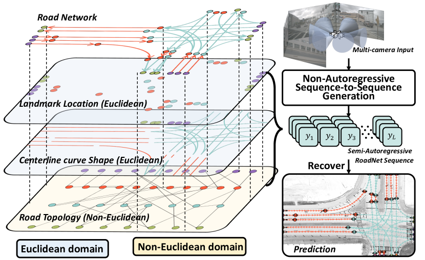
Figure 1: High-definition Road Network Topology contains Euclidean data: locations of landmarks and shapes of curves and non-Euclidean data: road topology. A special sequence, RoadNet Sequence, is proposed as a unified representation of both domains. Then we use a Non-Autoregressive sequence-to-sequence approach to extract RoadNet Sequence from multi-camera input efficiently and accurately.

With the rising prevalence of self-driving cars, a deep knowledge of the road structure is indispensable for autonomous vehicle navigation [15, 22, 39, 13]. Road network [12, 34, 37] extraction is required to estimate highly accurate road landmark locations, centerline curve shapes and road topological connection for self-driving vehicles. However, the ability to understand road network in real-time using onboard sensors is highly challenging.

In the literature, road network is differentiated from methods that focus solely on grid-like Euclidean data [6, 5] such as lane detection [55, 32, 56] or BEV semantic understanding [35, 45, 30, 33]. Instead, road network emphasizes a more comprehensive understanding of both Euclidean domain and non-Euclidean domain. As shown in Figure 1, accurate road landmark locations such as crossroads, stop-lines, fork-roads, and the shape of centerline curves pertain to the Euclidean domain, whereas road topology belongs to the non-Euclidean domain. In mathematical terms [5, 6], Euclidean data is defined in $\mathbb{R}^{2}$. On the other hand, non-Euclidean data, such as graphs that indicate connectivity among nodes, will lose crucial information if projected to $\mathbb{R}^{n}$, such as edge curve information.

Unfortunately, existing attempts [9, 10] to extract road network using onboard sensors have not been able to achieve a harmonious integration between Euclidean and non-Euclidean data. STSU [9] divides the road network construction into two stages: center-lines detection and center-line connectivity reasoning—which ignores the cooperation between Euclidean and non-Euclidean domains. TPLR [10] uses a Transformer or Polygon-RNN [1] to combine topology reasoning with center-line localization, but the embedded conflicts between Euclidean data representations and connectivity representation undermine the model performance.

In this work, we propose that the dilemma in existing works arises due to the absence of a unified representation of both Euclidean and non-Euclidean data. Instead, we introduce a Euclidean-nonEuclidean unified representation with merits of losslessness, efficiency and interaction. The unified representation, named as RoadNet Sequence, projects both Euclidean and non-Euclidean aspects of road network to integer series domain $\mathbb{Z}^{n}$. The “losslessness” aspect is ensured by establishing a bijection from road network to RoadNet Sequence. “Efficiency” is achieved by limiting RoadNet Sequence length to the shortest $\mathcal{O}(|\mathcal{E}|)$ (where $\mathcal{E}$ is the set of all centerlines), through a specially designed topological sorting rule. “Interaction” reveals the interdependence between Euclidean and non-Euclidean information within a single sequence.

Based on the auto-regressive dependency of topological sorting, we leverage the sequence-to-sequence generation power of Transformer [48, 7, 14] to understand RoadNet Sequence from onboard round-view cameras, called RoadNetworkTRansformer (RNTR).

However, in practice, the auto-regressive dependency in sequence-to-sequence generation can significantly slow down the inference speed. Our observation is that the dependency of road network can be decoupled into a semi-autoregressive format, that retains auto-regressive functionality within local contexts while simultaneously conducting multiple generations in parallel. This semi-autoregressive model is called Semi-Autoregressive RoadNetTransformer (SAR-RNTR). This approach not only accelerates the inference speed by 6 times, but it also significantly boosts the accuracy to a new level based on the better dependency modeling. Going beyond SAR-RNTR, we employ a masked training technique on SAR-RNTR to mimic the remaining auto-regressive dependency through iterative prediction [27]. This gives rise to our Non-Autoregressive RoadNetTransformer (NAR-RNTR) model, which achieves real-time inference speed ($47\times$ faster) while maintaining the high performance.

To evaluate road network extraction quality, apart from inheriting the former metrics [9] based on lane detection, we instead design a family of metrics directly based on definition of road network – Landmark Precision-Recall and Reachability-Precision-Recall – to evaluate (i) road landmarks localization accuracy, and (ii) path accuracy between any reachable landmarks.

We make the following contributions: (i) we introduce RoadNet Sequence, a lossless, efficient and unified representation of both Euclidean and non-Euclidean information from road network. (ii) We propose a Transformer-based RoadNetTransformer which can decode RoadNet Sequence from multiple onboard cameras. (iii) By decoupling auto-regressive dependency of RoadNet Sequence, our proposed Non-autoregressive RoadNetTransformer accelerate the inference speed to real-time while boost the accuracy with a significant step from the auto-regressive model. (iv) Extensive experiments on nuScenes [8] dataset validate the superiority of RoadNet Sequence representation and RoadNetTransformer over the alternative methods with a considerable margin.

2 Related work

Vision-based ego-car (BEV) feature learning A rising tendency is conducting self-driving downstream tasks [42, 30, 33, 24, 35, 45, 23, 29, 17, 31] under ego-car coordinate frame. To learn ego-car feature learning from onboard cameras,  [51, 38] project image features to ego-car coordinate based on depth estimation. OFT [42], LSS [35] and FIERY [23] predict depth distribution to generate the intermediate 3D representations. [45, 41, 30, 33] resort neural network like Transformer to learn ego-car feature without depth. In order to learn the topology of the road network under the ego-car coordinate frame, we use the straightforward method of applying LSS [35, 24] to extract ego-car features from the multiple onboard cameras.

Road network extraction Researchers have explored the utilization of DNNs to decode and recover maps from aerial images and GPS trajectories [43, 53]. Moreover, STSU [9] first detect centerline from front-view image with Transformer and then predict the association between centerline with MLP layer, followed with a final merge to estimate road network. Based on STSU, TPLR [10] introduces minimal cycle to eliminate ambiguity in its connectivity representation. Existing methods spend great effort to deal with problem in non-Euclidean domain but ignore the cooperation between Euclidean and non-Euclidean. However, we create a Euclidean-nonEuclidean unified representation.

Non-Autoregressvie generation Non-Autoregressive generation for Neural Machine Translation (NMT) [19] has been proposed as a solution to speed up the one-by-one sequential generation process of autoregressive models. [25, 57, 40] utilized knowledge distillation to help NAT model capture target sequence dependency. [27, 47, 20, 18] proposed iterative models that refine the output from the previous iteration or a noised target in a step-wise manner. [49] kept the auto-regressive approach for global modeling, but introduced the parallel output of a few successive words at each time step. [46, 4, 36, 3] used latent variables as intermediates to reduce the dependency on the target sequence. The current state of non-autoregressive NMT models is far from perfect, with a significant gap in performance compared to their auto-regressive counterparts [54]. But in the case of our RoadNet Sequence, the auto-regressive dependency can be decoupled, leading to both acceleration and improved performance.

3 Method

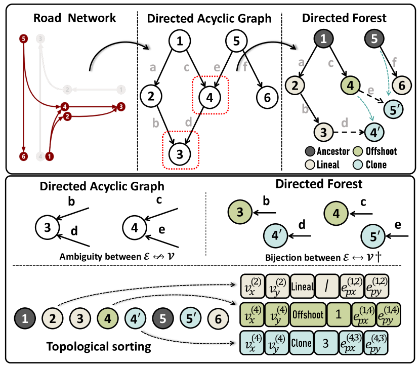
Figure 2: Top illustrates the transformation process from a Directed Acyclic Graph to a Directed Forest for RoadNet Sequence. The red boxes enclose all merge-points that have non-unique parents. We replicate theirs parents (except the first parent) to their children (cyan nodes) and delete the corresponding edges. Middle demonstrates a bijection between the edges and vertices (${\dagger}$: excluding the Ancestors). Bottom lists the topological sorting result of vertices and presents six integers for each vertex.

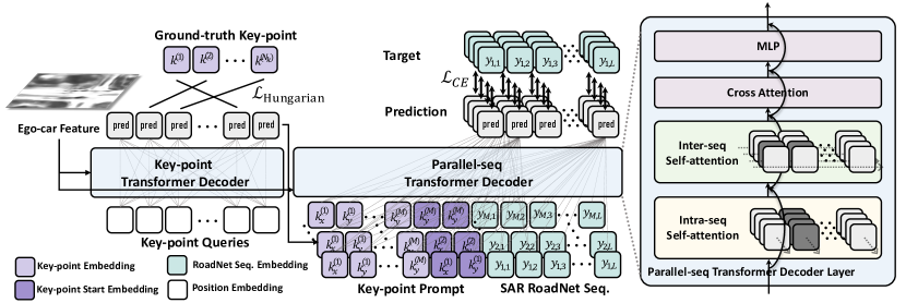
Figure 3: Left shows two major components of Semi-Autoregressive RoadNetTransformer: Key-point Transformer decoder to detect key-points and Parallel-seq Transformer Decoder to generate Semi-Autoregressive RoadNet Sequence. “SAR RoadNet Seq” stands for Semi-Autoregressive RoadNet Sequence. Right decouples self-attention of Parallel-seq Transformer Decoder layer into Intra-seq and inter-seq self-attention.

In this section, we will introduce: (i) mathematics modeling of road network, (ii) RoadNet Sequence, (iii) architecture of RoadNetTransformer, (iv) metrics.

3.1 Mathematics modeling of road network

The road network comprises road landmarks (e.g., crossroad, stop-lines, fork-point, merge-point) and centerlines connecting among them [9, 10]. Given that traffic on each lane is always one-way, the graph can be formulated as a Directed Acylic Graph (DAG), i.e., $\mathcal{G}=(\mathcal{V},\mathcal{E})$ where vertex set $\mathcal{V}$ is the set of all road landmarks and edge set $\mathcal{E}$ is the set of all centerlines. Each vertex $v=(v_{x},v_{y},v_{c})\in\mathcal{V}$ contains two properties: (i) location, i.e., $(v_{x}\in\mathbb{R},v_{y}\in\mathbb{R})$, (ii) category, i.e., $v_{c}$. As shown in Figure 2, we divide vertices into 4 categories which will be introduced later. Each edge $e=(e_{s},e_{t},e_{px},e_{py})\in\mathcal{E}$ contains two properties: (i) source $e_{s}\in\mathcal{V}$ and target $e_{t}\in\mathcal{V}$ vertex of the edge, (ii) Bezier middle control point $(e_{px}\in\mathbb{R},e_{py}\in\mathbb{R})$ [9] controlling the shape of edge curve. By and large, the Euclidean data of $\mathcal{G}$ contains $v_{x},v_{y},e_{px},e_{py}$ while the non-Euclidean data contains $v_{c},e_{s},e_{t}$.

3.2 RoadNet Sequence

In this section, we present RoadNet Sequence to integrate Euclidean and Non-Euclidean data into a unified representation. The projection from road network to RoadNet Sequence includes: (i) from DAG to Directed Forest, (ii) topological sorting of Directed Forest and (iii) sequence construction.

From DAG to Directed Forest A typical DAG always has the ambiguity relationship between vertices and edges ($|\mathcal{V}|\nleftrightarrow|\mathcal{E}|$) so that preserving all edges and vertices leads to redundancy due to the repeated use of vertices when indicating edge direction. In comparison, as shown in Figure 2, the Tree structure has a clear relationship between them ($|\mathcal{V}|\leftrightarrow|\mathcal{E}|$) which avoids this redundancy. Hence, we innovatively transform DAG to a Directed Forest $\mathcal{G}_{f}=(\mathcal{V}_{f},\mathcal{E}_{f})$ (a collection of disconnected directed trees). This transformation has the benefit of enabling us to find a bijection between $\mathcal{E}_{f}$ and $\mathcal{V}_{f}\backslash\{v\in\mathcal{V}_{f}\ |\ id(v)=0\}$ (set of all vertices which is not root, where $id(v)$ means incoming degree of the vertex). The bijection $f:\mathcal{V}\rightarrow\mathcal{E}$ can be $f(v)=(Parent(v),v)$ for any vertices $v\in\mathcal{V}_{f}\backslash\{v\in\mathcal{V}_{f}\ |\ id(v)=0\}$ where $Parent(v)$ is its unique parent and $f^{-1}(e)=v_{1}$ for any $e=(v_{0},v_{1})\in\mathcal{E}$.

As shown in the top of Figure 2, the transformation happens for all the merge-points on the road, i.e., $\{v\in\mathcal{V}\ |\ id(v)>1\}$ whose parents are non-unique. We replicate their parents (except the first parent) to their children and delete the corresponding edges. Then we assign these created vertices with a specific label Clone so that the direction of the edge between the merge-points and themselves will be reverted during recovery.

Topological sorting of Directed Forest We use Depth-first search (DFS) to obtain the sequential order of vertices $\mathcal{V}_{f}$ in the Directed Forest, i.e., $[v_{1},v_{2},\cdots,v_{n}]$. But the Clone point labeled in the last paragraph will not be traversed. Instead, as shown in the bottom of Figure 2, Clone point will be traversed following its original point.

Thanks to the bijection $f$ between $\mathcal{E}_{f}$ and $\{v\in\mathcal{V}_{f}\ |\ id(v)=1\}$, we can build pairs for all edges and vertices, i.e., $(v,f(v))$ for $v\in\{v\in\mathcal{V}_{f}\ |\ id(v)=1\}$ and $(v,\text{None})$ for $v\in\{v\in\mathcal{V}_{f}\ |\ id(v)=0\}$. These pairs construct the road network with no redundancy.

Non-unique sorting In the application of Depth-First Search (DFS), the sequence in which points under the same parent are searched first can result in non-unique sorting. We investigate two strategies to address this: a random ordering strategy and an ordering based on coordinates, specifically prioritizing points closest to the Bird’s Eye View (BEV) front right.

Sequence construction We then use 6 integers to represent each vertex-edge pair. 6 integers are made up with: (i) two integers for location of vertex, i.e., int$(v_{x})$, int$(v_{y})$; (ii) one integer for category $v_{c}$ of of vertex and we set categories as Ancestor, Lineal, Offshoot, Clone; (iii) one integer for the index of parent (None for root), $v_{d}=$Index$(Parent(v))$ where index is its topological order (the Clone vertex share the same index as origin to indicate that they are identical); (iv) two integers for coefficient of Bezier curve of $e=f(v)$, i.e.int$(e_{px})$, int$(e_{py})$. But, simply discretizing $e_{px}$ and $e_{py}$ can be challenging since the Bezier control points may exceed the Bird’s Eye View (BEV) range, and their values may become negative. As a solution, we discretize $e_{px}$ and $e_{py}$ by applying the int function to $(e_{px}+10)$ and $(e_{py}+10)$, respectively, to avoid negative values.

There exists 4 cases to determine the category $v_{c}$: (i) if $v_{i}$ is the root of the tree, the category $v_{c}$ is set as Ancestor, the index of its parent $v_{d}$ is set as None, its coefficient is ignored. (ii) if $v_{i}$ is the first child of its parent, the category $v_{c}$ is set as Lineal, its $v_{d}$ is ignored for its parent is exact $v_{i-1}$. (iii) if $v_{i}$ is not the first child of its parent, the category $v_{c}$ is set as Offshoot, its $v_{d}$ is its parent’s index. (iv) if $v_{i}$ is the cloned child, the category is set as Clone, its $v_{d}$ is its original child. Integer representation of $v_{c}$ is Ancestor: 0, Lineal: 1, Offshoot: 2, Clone: 3.

Analysis The proposed RoadNet Sequence possess the merits of losslessness, efficiency and interaction. The losslessness of RoadNet Sequence is guaranteed by establishing a bijection between edges and vertices (excluding the root) of trees. Our RoadNet Sequence has a complexity of $\mathcal{O}(|\mathcal{V}_{f}|)=\mathcal{O}(|\mathcal{E}|)$, making it the most efficient. A mixture of Euclidean and non-Euclidean data within a local 6-integer clause facilitates full interaction between the Euclidean and non-Euclidean domains.

RoadNet Sequence also possess the auto-regressive dependency. Since Depth-First search of Trees is always topological sorting, vertices only depend on the previous generated vertices. Also, our 6 integers come in the order of vertices location, vertices category, index and curve coefficient also preserving the auto-regressive assumption.

Sequence embedding Each vertex-edge pair is represented by 6 integers. To prevent embedding conflicts between the 6 integers, we divide them into separate ranges. As a default, we set the embedding size to $576$, which is sufficient to accommodate all the integer ranges.

3.3 Auto-Regressive RoadNetTransformer

Based on auto-regressive dependency of RoadNet Sequence, we design our baseline as auto-regressive  RoadNet Sequence generation.

Architecture We apply the same encoder-decoder architecture as [14]. The encoder is responsible for extracting BEV feature $\mathcal{F}$ from multiple onboard cameras such as Lift-Splat-Shoot [35]. For decoder, we use the same Transformer decoder as [14] which includes a self-attention layer, a cross-attention layer and a MLP layer.

Obejctive We denote the ground-truth RoadNet Sequence with length $L$ as $y$ and the predicted RoadNet Sequence as $\hat{y}$, then the objective of auto-regressive RoadNetTransformer is maximum likelihood loss, i.e.

$$\max\sum_{i=1}^{L}w_{i}\log{P(\hat{y}_{i}|y_{<i},\mathcal{F})}$$ (1)

where $y_{i}$ is the $i^{th}$ token of $y$, $y_{<i}$ means all tokens before $y_{i}$ and $w_{i}$ is the class weight. In practice, since the label Lineal for $v_{c}$ and index $0$ for $v_{d}$ appear most frequently, we set $w_{j}$ as a small value for these class.

Input and target sequence construction The input sequence starts with a start token and the target sequence ends with an EOS token. We also apply synthetic noise objects technique [14] to the sequence construction. Details are shown in the Supplementary material.

Efficiency Suppose the Transformer spends $\mathcal{T}_{s}$ time inferring a single query. The inference time complexity should be $\mathcal{O}(|\mathcal{E}|\cdot\mathcal{T}_{s})$.

3.4 Semi-autoregressive RoadNetTransformer

The vanilla Auto-Regressive RoadNetTransformer generates RoadNet Sequence one by one, which is a highly time-consuming process. The reason for this expensive one-by-one generation is the ingrained auto-regressive dependency assumption.

In the field of Natural Language Processing, the human language is highly cohesive, which means that any attempt to generate text without auto-regressive assumption can result in a significant decrease in accuracy [54]. However, it’s not the case for road network. With regards to the Figure 1, observations have been made regarding the dependency of RoadNet Sequence: (i) The locations of certain road points (start points, fork points or merge points) can be independent of previous vertices and instead depend solely on the BEV feature map, i.e.,

$$P(y_{i}|y_{<i},\mathcal{F})=P(y_{i}|\mathcal{F})$$ (2)

(ii) Except for locations of these road points, other tokens are still strongly auto-regressive.

Drawing from these findings, we suggest the adoption of Semi-autoregressive RoadNetTransformer (SAR-RNTR) that retains auto-regressive functionality within local contexts while simultaneously conducting none-autoregressive generations in parallel. To facilitate this approach, we propose a novel representation of the road graph called Semi-Autoregressive RoadNet Sequence.

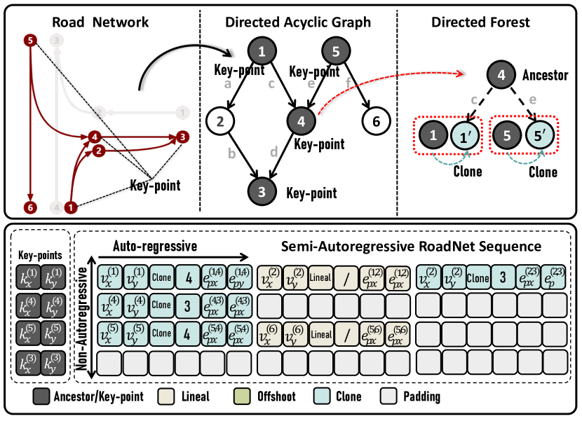
Figure 4: Top indicates the selection of key-points and the approach to construct sub-trees taking these key-points as root. Bottom presents the Semi-Autoregressive RoadNet Sequence for the example mentioned above.

Semi-Autoregressive RoadNet Sequence The objective of Semi-Autoregressive RoadNet Sequence is to divide the trees in the Directed Forest into smaller sub-trees as much as possible so that each tree will be simultaneously inferred and the auto-regressive length can be reduced as much as possible. As shown in Figure 4, we begin by identifying all key-points in the Directed Acyclic Graph (DAG) that meet the condition $od(v)>1$ or $id(v)>1$ or $id(v)=0$. We then proceed to recursively extract these points from their original parent and sub-tree until they become roots with an $id(v)$ value of 0. To restore the edge between the key-point $v$ and its parent, we create a duplicate of the parent and assign it as the child of $v$ with a special label, Clone, identical to that used in RoadNet Sequence. Similarly, the Clone will only be traversed after its original vertex is traversed. As shown in Figure 4, different from the auto-regressive RoadNet Sequence, we construct an independent sequence for each independent tree, so that the SAR-RoadNet Sequence is a 2-dimension sequence, i.e., $[[y_{1,1},y_{1,2},\cdots,y_{1,L}],\cdots,[y_{M,1},y_{M,2},\cdots,y_{M,L}]]$, where $L$ is the maximum length of each sub-sequence and $M$ is the number of sub-sequences. The padding rules is shown in the Supplementary material. Noted that the new data structure is also a directed forest, therefore the construction and recovering follow all rules in the auto-regressive RoadNet Sequence.

Architecture The SAR-RNTR can be divided into three parts: (i) Ego-car Feature Encoder, (ii) Key-point Transformer Decoder, (iii) Parallel-Seq Transformer Decoder. Ego-car Feature Encoder follows that in AR-RNTR. Key-point Transformer Decoder is a parallel Transformer decoder [11], which takes a fixed set of learned positional embeddings as input and predict locations of key points based on set prediction [11].

Then, Parallel-Seq Transformer Decoder is proposed for solving mixture of auto-regressive and non-autoregressive problem, i.e..

$$\max\sum_{i=1}^{M}\sum_{j=1}^{L}P(y_{i,j}\ |\ y_{1:M,1:j-1},\mathcal{F},\mathcal{V}_{kp}),$$ (3)

where $\mathcal{V}_{kp}$ represents location of key-points detected from Key-points Transformer Decoder. For a certain $i$, $y_{i,j}$ is generated auto-regressively, while for a certain $j$, all $y_{1:M,j}$ are generated in parallel. The dependency is illustrates in Figure 3.

However, following this objective will cost $\mathcal{O}(M^{2}\times L^{2})$ memory complexity for self-attention [48]. Inspired by [50], where a cross combination of self-attention from different directions leads to a final global attention, we design two self-attention applied on different directions of the 2-dimension Semi-Autoregressive RoadNet Sequence. As shown in Figure 3, Intra-seq self-attention first applies self-attention on $y_{1:M,j}$ for each $j$ and Inter-seq self-attention then applies self-attention on $y_{i,1:j-1}$ for each $i$. The memory complexity is reduced to $\mathcal{O}(M^{2}+L^{2})\ll\mathcal{O}(M^{2}\times L^{2})$.

Key-point Prompt Learning To deduce $y_{i,1:L}$ using $\mathcal{V}_{kp}$ as a basis according to Equation 3, we implement Key-point Prompt Learning. Key-point Prompt for a sub sequence $y_{i,1:L}$ contains two parts: (i) locations of all key-points; (ii) location of the start key-point (Ancestor) of $y_{i,1:L}$. As depicted in Figure 3, this involves organizing the locations of key-points and the start key-point location as a sequence of discrete tokens, and assigning dedicated word embeddings and position embedding for the prompt. The Key-point Prompt is then added to Semi-Autoregressive RoadNet Sequence facilitates the aggregation of key-point information in the sequence.

Objective The objective contains two part: key-points detection and auto-regressive MLE loss. Key-points are optimized by Hungarian loss [11]. We denote the set of $M$ predictions as $\hat{z}=\{\hat{z}^{(i)}\}_{i=1}^{M}$, and the ground-truth $z$. Each $z_{i}$ composes $z^{(i)}=(c^{(i)},k^{(i)})$, where $c^{(i)}\in\{0,1\}$ denotes whether the prediction is a key-point and $k^{(i)}=(k^{(i)}_{x},k^{(i)}_{y})$ is the position of key-points. We then build the pair-wise matching cost $\mathcal{L}_{\text{match}}(z_{i},\hat{z}_{\sigma(i)})$ between ground-truth $z_{i}$ and prediction $z_{\sigma(i)}$. We define the matching cost as class probability and key-points L-1 distance, i.e.$\mathcal{L}_{\text{match}}(z_{i},\hat{z}_{\sigma(i)})$ as $-\mathbb{1}_{\{c_{i}\neq 0\}}\hat{p}_{\sigma(i)}(c_{i})+\mathbb{1}_{\{c_{i}\neq 0\}}\|k^{(i)}-\hat{k}^{(i)}\|_{1}$. Based on this matching cost, we find a bipartite matching between these two sets with the lowest matching cost.

The second step is to compute the Hungarian loss for all pairs matched in the previous step. The Hungarian loss is a linear combination of a negative log-likelihood for class prediction and a L-1 loss.

$$\mathcal{L}_{\text{Hungarian}}(z,\hat{z}) =\sum_{i=1}^{M}\left[-\log{\hat{p}_{\sigma(i)}(c_{i})}\right.$$

$$+\left.\mathbb{1}_{\{c_{i}\neq 0\}}\|k^{(i)}-\hat{k}^{(i)}\|_{1}\right]$$ (4)

Auto-regressive MLE loss follows that of AR-RNTR.

Efficiency and dependency Suppose the Transformer spends $\mathcal{T}_{s}$ time inferring a single query, and the parallel acceleration rate for GPU is $\alpha\ll 1$. The inference time complexity of combination of Key-point and Parallel-seq Transformer can be approximated as $\mathcal{O}(\alpha(|\mathcal{E}|+|\mathcal{V}_{kp}|)\cdot\mathcal{T}_{s})$ which greatly less than that of Auto-Regressive by ratio $\alpha(1+\frac{|\mathcal{V}_{kp}|}{|\mathcal{E}|})$. In addition to acceleration, improved dependency modeling can also enhance contextual reasoning [58, 52, 2], thus benefiting performance.

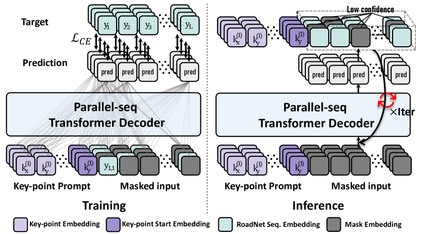
Figure 5: Left illustrates the training stage which takes masked (gray square) Semi-Autoregressive RoadNet Sequence as input. Right shows inference stage where the Parallel-seq Transformer Decoder takes a fully-masked sequence as input and iteratively masks the predicted token with low confidence.

3.5 Non-Autoregressive RoadNetTransformer

While the Semi-autoregressive RoadNetTransformer improves inference speed to some extent, there is still an inefficient auto-regressive component present. Therefore, we propose a fully non-autoregressive generation model, called Non-Autoregressive RoadNetTransformer, which can output the entire sequence at once. To mimic the auto-regressive generation, we iteratively refine the output from this non-autoregressive generation , i.e.,

$$\max\sum_{i=1}^{M}\sum_{j=1}^{L}P(y_{i,j}\ |\ \hat{y},\mathcal{F},\mathcal{V}_{kp}),$$ (5)

where $\hat{y}$ is the predicted Semi-Autoregressive RoadNet Sequence of the last guess. Provided the limited iteration times, the Non-Autoregressive RoadNetTransformer can achieve a extremly high inference speed than its auto-regressive counterpart.

The training and inference approach are visualized in Figure 5. During training, we utilize a masked language modeling strategy [16] that involves masking a high percentage of the input ground-truth sequence and prompting the Transformer to predict all the missing tokens. Thus, during inference, we begin with a fully masked sequence and predict the Semi-Autoregressive RoadNet Sequence multiple times, with each iteration masking tokens with low confidence. With each iteration, the results will be gradually refined.

Efficiency Time complexity for NAR-RNTR can be approximated as $\mathcal{O}(\alpha|\mathcal{V}_{kp}|(N_{iter}+1)\cdot\mathcal{T}_{s})$. Acceleration ratio is $\frac{|\mathcal{E}|/|\mathcal{V}_{kp}|+1}{N_{iter}+1}$ where $N_{iter}\ll|\mathcal{E}|/|\mathcal{V}_{kp}|$.

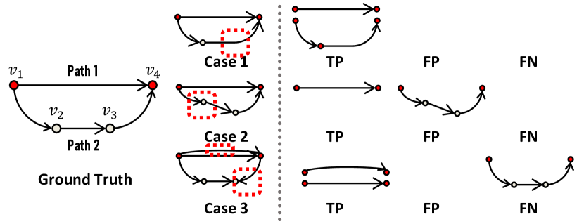
Figure 6: Examples of TP, FP and FN when evaluating reachability between $v_{1}$ and $v_{4}$. Although case 1 misses landmark $v_{2}$, but both paths between $v_{1}$ and $v_{4}$ are within distance of the ground-truth paths. Case 2, however, has path 2 surpasses the threshold distance from matched its matched ground-truth path 2 so it’s false positive. Case 3 predicts path 1 twice but they are both within threshold distance. However, path 2 in the ground-truth has no matched prediction so it’s false negative.

3.6 Metrics

Precision-Recall Precision is defined as

$$\text{Precision}=\frac{\text{True Positive}}{\text{True Positive}+\text{False Positive}}$$ (6)

Recall is defined as

$$\text{Recall}=\frac{\text{True Positive}}{\text{True Positive}+\text{False Negative}}$$ (7)

And F1 score is defined as

$$\text{F1 score}=\frac{2\times\text{Precision}\times\text{Recall}}{\text{Precision}+\text{Recall}}$$ (8)

To ensure a fair comparison, we employ three metrics from [9, 10]: Mean Precision-Recall, Detection ratio, and Connectivity. However, these metrics, which rely solely on centerline detection, neglect the significance of both the location accuracy of road-points and the reachability of the road graph. To make up with the deflect, we propose 2 following metrics.

Landmark Precision-Recall We use Landmark Precision-Recall to evaluate the location accuracy of landmarks. For each predicted landmark, we match it to a ground-truth with the nearest distance. If a predicted landmark is within the threshold distance with its matched ground-truth, it is true positive, otherwise it is false positive. If a ground truth landmark is not matched with any predictions or not within the threshold distance with its matched prediction, it is false negative. Thresholds for Landmark Precision-Recall are chosen from $[0.5,1.0,1.5,2.0,2.5,$ $3.0,3.5,4.0,4.5,5.0]m$.

Reachability Precision-Recall One of the motivations for predicting road topology is finding the valid paths of any two points on the road, which allows the self-driving car to reach its destination. Reachability between landmarks is defined that there exists a path going from one landmark to another. After matching landmarks in the former session, we propose reachability precision-recall to evaluate both connectivity and accuracy of path between landmarks. In the road network, if two landmarks are connected, it means there exists a path from one landmark to another. Given a pair of predicted landmarks $\hat{A},\hat{B}$ and its matched pair of ground-truth landmarks $A,B$, a true positive is a path connecting $\hat{A},\hat{B}$ with Chamfer Distance to any of the ground-truth path connecting $A,B$ less than the threshold. A false negative is a ground truth path from $A,B$ with no matched predicted path. Thresholds for Reachability Precision-Recall are chosen from $[0.5,1.0,1.5,2.0,2.5]m$. An example is given in Figure 6.

4 Experiments

4.1 dataset

We utilize the nuScenes [8] dataset (700/150/150 for training/validation/test) to assess our approach. We only utilize sensor information from six cameras, IMU, and GPS, which were sampled at a rate of 2Hz.

4.2 Implementation

Pretrain We follow LSS [35] for BEV Encoder. The input images are resized to $128\times 352$, and the target BEV area is from -48 to 48m in x-direction (roll) and -32 to 32m in y-direction (pitch) with resolution $1$m in ego coordinate system. ResNet-50 [21] or VoVNetV2 [28] are used as image backbone. Initially, we pretrain the BEV encoder on centerline segmentation, following all the training strategy outlined in LSS [35]. During training of RoadNetTransformer, we load and freeze the parameters of BEV encoder.

RoadNetTransformer Details of three variants are shown below. AR-RNTR: The length of RoadNet Sequence is padded to $6\times 100$. Transformer decoder layers of AR-RNTR is set as 6. Our AR-RNTR is trained on 300 epochs with learning rate $2\times 10^{-4}$, batch size as $2\times 8$. During the training process, we apply random flip, random rotation and random scaling on BEV feature similar to [24, 33]. SAR-RNTR: Transformer decoder layers of SAR-RNTR is set as 6 (Key-point) plus 3 (Parallel-seq). We use noise vertices to pad all sub-sequences to the length of $6\times 18$, and the max number of key-points is set to 34. The strategies for data augmentation and training are the same as AR-RNTR. NAR-RNTR: During training, we load parameter of trained SAR-RNTR and then finetune it with mask language modeling strategy for 100 extra epochs. During inference, iteration number is set to 3.

Metrics Thresholds for Mean Precision-Recall and Landmark Precision-Recall are uniformly sampled from $[0.5,5.0]$ m. Thresholds for Reachability Precision-Recall are uniformly sampled from $[0.5,2.5]$ m. We only take into account the reachability between vertices that are within a maximum of 5 edges of connection.

4.3 Results

Methods	M-P	M-R	M-F	Detect	C-P	C-R	C-F
PINET [26]	54.1	45.6	49.5	19.2	-	-	-
Poly [1]	54.7	51.2	52.9	40.5	58.4	16.3	25.5
STSU [9]	60.7	54.7	57.5	60.6	60.5	52.2	56.0
TPLR [10]	-	-	58.2	60.2	-	-	55.3
AR-RNTR	60.9	57.9	59.3	61.7	63.2	52.7	57.5
SAR-RNTR	63.5	59.9	61.6	63.5	67.1	57.2	61.7
NAR-RNTR	62.0	59.4	60.7	62.0	66.4	56.2	60.9

Table 1: Comparison of front-camera road network extraction with state of the art on nuScenes [8] PON validation split [41]. ResNet-50 [21] is applied as image backbone by default. M-P, M-R, M-F stand for mean precision/recall/F1-score [9]. Detect stands for Detection ratio metrics [9]. C-P, C-R, C-F stand for connectivity precision/recall/F1-score [9].

Comparison with state of the art We compare our model with previous state-of-the-art methods on high-definition road network topology extraction. To achieve a fair comparison, we only utilize front-view images as input and ResNet-50 [21] trained on ImageNet-1K [44] as backbone. Also, we utilize the PON nuScenes train/val split [41] as also applied in [9, 10]. Table 1 presents the results of our approach on the nuScenes dataset using the Mean Precision-Recall, Detection, and Connectivity metrics [9]. On the one hand, our model outperforms all three variants across all metrics, demonstrating the superior performance of RNTR in both centerline detection and centerline association estimation. This remarkable improvement on both centerline location and connectivity can be attributed to the unified representation provided by RoadNet Sequence and the global context reasoning capabilities of the Transformer architecture.

On the other hand, unlike in Natural Language Processing, our Semi-Autoregressive and Non-Autoregressive version significantly outperforms the Auto-Regressive version, highlighting our dependency decoupling.

Methods	Landmark			Reachability			FPS
	L-P	L-R	L-F	R-P	R-R	R-F
NAR-RNTR	57.1	42.7	48.9	63.7	45.2	52.8	5.5
AR-RNTR†	62.6	47.9	54.3	73.2	52.9	61.4	0.1 (1.0$\times$)
SAR-RNTR†	66.0	55.9	60.5	74.5	61.1	67.1	0.6 (6.0$\times$)
NAR-RNTR†	65.6	55.7	60.2	73.4	60.0	66.0	4.7 (47$\times$)

Table 2: Comparison of multiple-camera road network extraction on nuScenes [8] dataset assessed by Landmark Precision-Recall (L-P, L-R, L-F) and Reachability Precision-Recall (R-P, R-R, R-F). ResNet-50 [21] is applied as image backbone by default. “†” use VoVNetV2 [28] pretrained on extra data as backbone. FPS is tested on NVIDIA V100.

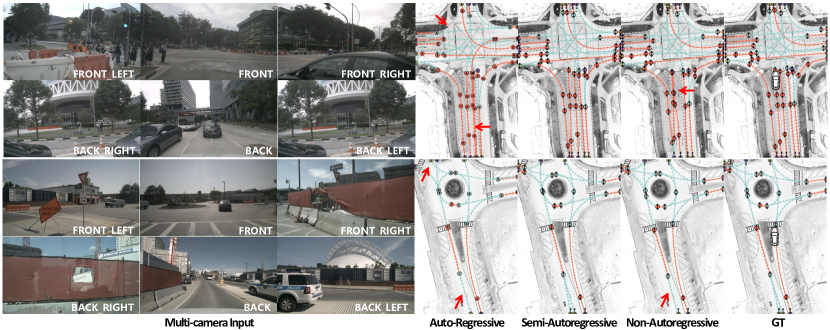
Figure 7: Qualitative results on nuScenes validation set. All three variants of RoadNetTransformer predict high quality road network. Only slight errors (pointed by red arrow) occur when predicting landmarks locations for AR-RNTR and NAR-RNTR.

Landmark and Reachability Table 2 evaluate our methods on Landmark Precision-Recall and Reachability Precision-Recall. The auto-regressive RNTR performs worst in most metrics without saying it’s slowest inference speed. In comparison, the Semi-Autoregressive RNTR leads in all metrics, and boosts the inference speed by 6.0 times. Remarkably, the non-autoregressive version of RNTR outperforms the AR-RNTR in all metrics and dramatically improves inference speed by a factor of 47$\times$, surpassing the nuScenes camera sampling frequency of 2Hz and enabling real-time inference. The small gap between NAR-RNTR and SAR-RNTR proves the feasibility of the masked sequence training and the iterative based inference. To summarize, the SAR-RNTR achieves the best performance, while the NAR-RNTR strikes a very balance between efficiency and accuracy.

4.4 Ablation studies

We conduct ablation studies on Transformer layer numbers, as well as mask ratio and iteration times of NAR-RNTR during inference.

# Key-pt	# Para-Seq	Intra-Seq	L-F	R-F	FPS
3	3	✓	56.1	63.3	4.8
5	3	✓	58.2	65.1	4.8
6	3	✓	60.2	66.0	4.7
6	5	✓	60.5	66.9	3.4
6	6	✓	61.3	67.1	3.0
6	3	✗	55.7	56.3	5.0

Table 3: Ablation studies on number of Transformer decoder layers and Intra-seq self-attention of NAR-RNTR. # Key-pt denotes Key-point Transformer Decoder layer number, and # Para-seq denotes Parallel-seq Transformer Decoder layer number. Intra-Seq means Intra-seq self-attention in Parallel-seq Transformer Decoder layer. VoVNetV2 [28] pretrained on extra data is applied as image backbone by default. The row with gray color is our final choice.

Number of Transformer layers We investigated the impact of the number of Transformer layers on NAR-RNTR in Table 3. Using fewer Key-point Transformer decoder layers leads to a significant loss in accuracy for both landmark and reachability, but provides limited speed-up. Conversely, using fewer Parallel-seq Transformer decoder layers dramatically improves inference speed while incurring less accuracy loss.

Intra-Seq self-attention The bottom row of Table 3 highlights the crucial role of Intra-seq self-attention. Its absence results in a significant loss in both landmark localization and topology connection.

Mask ratio	# iteration	L-F	R-F	FPS
50%	3	51.4	51.3	4.7
75%	3	59.4	62.7	4.7
90%	1	59.0	62.7	8.9
90%	3	60.2	66.0	4.7
90%	6	60.3	66.1	2.8

Table 4: Ablation studies on mask ratio and iteration times of NAR-RNTR. VoVNetV2 [28] pretrained on extra data is applied as image backbone by default. The row with gray color is our final choice.

Mask ratio and iteration times Our investigation into the impact of the mask ratio during training of NAR-RNTR revealed the importance of using a large mask ratio. Consequently, a 90% mask ratio is used during Non-Autoregressive finetuning. We also observed accuracy saturation as the number of iterations increased. Therefore, we used 3 iterations for our approach.

4.5 Qualitative results

We present our visualization in Figure 7. The precise localization of landmarks, accurate topological connections, and precise curve shapes demonstrate the superiority of RoadNetTransformer. Additional qualitative results are presented in the Supplementary material.

5 Conclusion and Limitation

In summary, our work introduces a lossless, efficient and interactional sequence representation called RoadNet Sequence, which preserves both Euclidean and non-Euclidean data of road networks. We have designed an Auto-Regressive RoadNetTransformer as a baseline model, which takes advantage of the auto-regressive dependency of RoadNet Sequence. Additionally, we have proposed Semi-Autoregressive and Non-Autoregressive RoadNetTransformer models, which decouple the auto-regressive dependency of RoadNet Sequence, resulting in significantly faster inference speeds and improved accuracy. Our extensive experiments demonstrate the superiority of our RoadNet Sequence representation and RoadNetTransformer models.

In terms of limitation, the Transformer decoder of AR-RNTR is effective but computationally expensive as the complexity of RoadNet Sequence is $\mathcal{O}(|\mathcal{E}|)$, resulting in a cost increase of $\mathcal{O}(|\mathcal{E}|^{2})$. In contrast, both SAR-RNTR and NAR-RNTR offer enhanced efficiency. However, the specifically designed Semi-Autoregressive RoadNet Sequence truncates the scalability

Appendix A Appendix

A.1 RoadNet Sequence & Semi-Autoregressive RoadNet Sequence

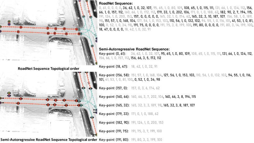
Figure 10: Left shows topological order of RoadNet Sequence and Semi-Autoregressive RoadNet Sequence. Right shows original RoadNet Sequence and Semi-Autoregressive RoadNet Sequence without input/target processing.

Details of sequence construction The discretization of $v_{x},v_{y}$ is simply truncating the integer part. Integer representation of $v_{c}$ is Ancestor: 0, Lineal: 1, Offshoot: 2, Clone: 3. Discretizing $e_{px}$ and $e_{py}$ can be challenging since the Bezier control points may exceed the Bird’s Eye View (BEV) range, and their values may become negative. As a solution, we discretize $e_{px}$ and $e_{py}$ by applying the int function to $(e_{px}+10)$ and $(e_{py}+10)$, respectively, to avoid negative values. Figure 10 shows a example of both RoadNet Sequence and Semi-Autoregressive RoadNet Sequence.

A.2 Input and target sequence construction

Sequence embedding Each vertex-edge pair is represented by 6 integers. To prevent embedding conflicts between the 6 integers, we divide them into separate ranges which is shown in Table 5. As a default, we set the embedding size to $576$, which is sufficient to accommodate all the integer ranges.

Item	Range
$v_{x},v_{y}$	$0\sim 199$
$v_{c}$	$200\sim 249$
$v_{d}$	$250\sim 349$
$e_{px},e_{py}$	$350\sim 569$
noise category	$570$
EOS	$571$
Start	$57$2
n/a	$573$

Table 5: Embedding range of different integers.

Synthetic noise objects technique The input sequence of RoadNet Sequence starts with a start token and the target sequence ends with an EOS token. The EOS token makes the model know where the sequence terminates, but the experiments have shown that it tends to cause the model to stop predicting early without getting the complete sequence. Inspired by [14], we use a similar sequence augmentation technique to alleviate the problem called the synthetic noise objects technique [14]. The technique composes of sequence augmentation and sequence noise padding. The sequence augmentation adds noise to the position of landmarks and the coefficient of centerlines in input sequence. Whereas, sequence noise padding is a padding technique. For input sequences, we generate synthetic noise vertices and append them at the end of the real vertices sequence. Each noise vertex includes random locations($v_{x}$, $v_{y}$), category($v_{c}$), index of parent($v_{d}$) and Bezier curve coefficient($e_{px}$, $e_{py}$). As for the target sequence, the EOS token is added to the end of the real vertices sequence. We set the target category($v_{c}$) of each noise vertex to a specific noise class(different from any of the ground-truth labels), and the remaining components($v_{x}$, $v_{y}$, $v_{d}$, $e_{px}$, $e_{py}$) of the noise vertex to the ”n/a” class, whose loss is not calculated in the back-propagation.

However, we only use sequence noise padding as sequence augmentation has been shown to cause a decrease in performance. The introduced modifications of the synthetic noise objects technique are illustrated in Figure 8

The padding rules of Semi-Autoregressive RoadNet Sequence are much the same as auto-regressive RoadNet Sequence. As mentioned in the main submission, we pad the 2-dimensional Semi-Autoregressive RoadNet Sequence to $[[y_{1,1},y_{1,2},\cdots,y_{1,L}],\cdots,[y_{M,1},y_{M,2},\cdots,y_{M,L}]]$, where $L$ is the maximum length of each sub-sequence and $M$ is the number of sub-sequences. The valid sub-sequences begin with a key-point. For each valid sub-sequence, we follow the same padding rules of RoadNet Sequence, except there isn’t a start token in an input sub-sequence because of the Key-point Prompt. We set the other sub-sequences to the ”n/a” class making the loss of these sub-sequences without a key-point not calculated.

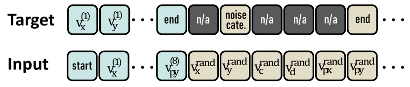
Figure 8: An illustration of synthetic noise objects technique [14] on RoadNet Sequence. Loss weight for n/a tokens are set to zero. Noise cate. stands for noise category.

BEV Aug	Sequence Aug	Sequence Noise	L-F	R-F
✓	✗	✗	58.6	64.3
✗	✗	✓	57.5	62.7
✓	✗	✓	60.2	66.0
✓	✓	✓	59.1	65.2

Table 6: Ablation studies on BEV augmentation and synthetic noise objects [14] (including sequence augmentation and sequence noise padding). NAR-RNTR with VoVNetV2 [28] pretrained on extra data is applied. The row with gray color is our final choice.

Embedding size	class weight	L-F	R-F
576	1.0	60.1	65.5
576	0.5	60.1	66.1
576	0.1	60.2	66.0
576	0.2	60.2	66.0
1000	0.2	60.1	65.8
2000	0.2	59.7	65.5

Table 7: Ablation studies on sequence embedding size and class weight. NAR-RNTR with VoVNetV2 [28] pretrained on extra data is applied. The row with gray color is our final choice.

Thresholds for Reachability Precision-Recall are chosen from $[0.5,1.0,1.5,2.0,2.5]m$.

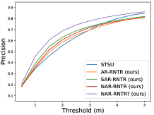
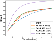
Figure 9: Mean Precision/Recall v.s. thresholds. Data of STSU [9] is recorded from Figure 7 of [9]. “${\dagger}$” use VoVNetV2 [28] pretrained on extra data as backbone. Thresholds are from $[0.5,1.0,1.5,2.0,2.5,3.0,3.5,4.0,4.5,5.0]m$.

A.3 Precision-Recall curve

In addition to our overall advantage in mean Precision-Recall (as presented in Table 1 of the main submission), Figure 9 displays the precision/recall versus thresholds curve. Our models outperform others in terms of precision and recall for smaller thresholds, highlighting our accuracy advantage.

A.4 Ablation studies

Non-unique Sorting We show the difference between the random ordering strategy and an ordering based on coordinates in Table

BEV augmentation The first column of Table 6 shows that the BEV augmentation provides a significant 2.7/3.3 improvement on both Landmark and Reachability scores.

Synthetic noise objects The second column of Table 6 shows that the sequence augmentation of Synthetic noise objects technique [14], however, leads to a drop in performance. Whereas, the third column shows that the sequence noise padding 1.6/1.7 improved on both Landmark and Reachability scores. But the sequence noise padding is less effective than BEV augmentation.

Class weight We exam the class weight for MLE loss, i.e., $w$ for

$$\max\sum_{i=1}^{L}w_{i}\log{P(\hat{y}_{i}|y_{<i},\mathcal{F})},$$ (9)

$$\max\sum_{i=1}^{M}\sum_{j=1}^{L}w_{j}P(y_{i,j}\ |\ \hat{y},\mathcal{F},\mathcal{V}_{kp}),$$ (10)

Due to the high frequency of Lineal for $v_{c}$ and the default index for $v_{d}$, we assign a lower weight to these categories. Although the second column of Table 7 does not indicate a clear relationship between class weight and performance, using a lower weight for the loss results in more stable performance.

Embedding size If we extend the embedding size from 576 to 1000 or 2000, useless embeddings clearly harm the performance.

References

- [1] David Acuna, Huan Ling, Amlan Kar, and Sanja Fidler. Efficient interactive annotation of segmentation datasets with polygon-rnn++. In CVPR, 2018.
- [2] Xuyang Bai, Zeyu Hu, Xinge Zhu, Qingqiu Huang, Yilun Chen, Hongbo Fu, and Chiew-Lan Tai. Transfusion: Robust lidar-camera fusion for 3d object detection with transformers. In CVPR, 2022.
- [3] Yu Bao, Shujian Huang, Tong Xiao, Dongqi Wang, Xinyu Dai, and Jiajun Chen. Non-autoregressive translation by learning target categorical codes. In NAACL, 2021.
- [4] Yu Bao, Hao Zhou, Shujian Huang, Dongqi Wang, Lihua Qian, Xinyu Dai, Jiajun Chen, and Lei Li. Glat: Glancing at latent variables for parallel text generation. In ACL, 2022.
- [5] Michael M Bronstein, Joan Bruna, Taco Cohen, and Petar Veličković. Geometric deep learning: Grids, groups, graphs, geodesics, and gauges. arXiv preprint, 2021.
- [6] Michael M Bronstein, Joan Bruna, Yann LeCun, Arthur Szlam, and Pierre Vandergheynst. Geometric deep learning: going beyond euclidean data. IEEE Signal Processing Magazine, 34(4):18–42, 2017.
- [7] Tom Brown, Benjamin Mann, Nick Ryder, Melanie Subbiah, Jared D Kaplan, Prafulla Dhariwal, Arvind Neelakantan, Pranav Shyam, Girish Sastry, Amanda Askell, et al. Language models are few-shot learners. In NeurIPS, 2020.
- [8] Holger Caesar, Varun Bankiti, Alex H Lang, Sourabh Vora, Venice Erin Liong, Qiang Xu, Anush Krishnan, Yu Pan, Giancarlo Baldan, and Oscar Beijbom. nuscenes: A multimodal dataset for autonomous driving. In CVPR, 2020.
- [9] Yigit Baran Can, Alexander Liniger, Danda Pani Paudel, and Luc Van Gool. Structured bird’s-eye-view traffic scene understanding from onboard images. In CVPR, 2021.
- [10] Yigit Baran Can, Alexander Liniger, Danda Pani Paudel, and Luc Van Gool. Topology preserving local road network estimation from single onboard camera image. In CVPR, 2022.
- [11] Nicolas Carion, Francisco Massa, Gabriel Synnaeve, Nicolas Usunier, Alexander Kirillov, and Sergey Zagoruyko. End-to-end object detection with transformers. In ECCV, 2020.
- [12] Sergio Casas, Abbas Sadat, and Raquel Urtasun. Mp3: A unified model to map, perceive, predict and plan. In CVPR, 2021.
- [13] Dian Chen, Brady Zhou, Vladlen Koltun, and Philipp Krähenbühl. Learning by cheating. In CORL, 2020.
- [14] Ting Chen, Saurabh Saxena, Lala Li, David J Fleet, and Geoffrey Hinton. Pix2seq: A language modeling framework for object detection. In ICLR, 2021.
- [15] Henggang Cui, Vladan Radosavljevic, Fang-Chieh Chou, Tsung-Han Lin, Thi Nguyen, Tzu-Kuo Huang, Jeff Schneider, and Nemanja Djuric. Multimodal trajectory predictions for autonomous driving using deep convolutional networks. In ICRA, 2019.
- [16] Jacob Devlin, Ming-Wei Chang, Kenton Lee, and Kristina Toutanova. Bert: Pre-training of deep bidirectional transformers for language understanding. arXiv preprint, 2018.
- [17] Jiyang Gao, Chen Sun, Hang Zhao, Yi Shen, Dragomir Anguelov, Congcong Li, and Cordelia Schmid. Vectornet: Encoding hd maps and agent dynamics from vectorized representation. In CVPR, 2020.
- [18] Marjan Ghazvininejad, Omer Levy, Yinhan Liu, and Luke Zettlemoyer. Mask-predict: Parallel decoding of conditional masked language models. In EMNLP-IJCNLP, 2019.
- [19] Jiatao Gu, James Bradbury, Caiming Xiong, Victor OK Li, and Richard Socher. Non-autoregressive neural machine translation. In ICLR, 2018.
- [20] Jiatao Gu, Changhan Wang, and Junbo Zhao. Levenshtein transformer. In NeurIPS, 2019.
- [21] Kaiming He, Xiangyu Zhang, Shaoqing Ren, and Jian Sun. Deep residual learning for image recognition. In CVPR, 2016.
- [22] Joey Hong, Benjamin Sapp, and James Philbin. Rules of the road: Predicting driving behavior with a convolutional model of semantic interactions. In CVPR, 2019.
- [23] Anthony Hu, Zak Murez, Nikhil Mohan, Sofía Dudas, Jeffrey Hawke, Vijay Badrinarayanan, Roberto Cipolla, and Alex Kendall. Fiery: future instance prediction in bird’s-eye view from surround monocular cameras. In ICCV, 2021.
- [24] Junjie Huang, Guan Huang, Zheng Zhu, and Dalong Du. Bevdet: High-performance multi-camera 3d object detection in bird-eye-view. arXiv preprint, 2021.
- [25] Yoon Kim and Alexander M. Rush. Sequence-level knowledge distillation. In EMNLP, 2016.
- [26] Yeongmin Ko, Younkwan Lee, Shoaib Azam, Farzeen Munir, Moongu Jeon, and Witold Pedrycz. Key points estimation and point instance segmentation approach for lane detection. IEEE Transactions on Intelligent Transportation Systems, 23(7):8949–8958, 2021.
- [27] Jason Lee, Elman Mansimov, and Kyunghyun Cho. Deterministic non-autoregressive neural sequence modeling by iterative refinement. In EMNLP, 2018.
- [28] Youngwan Lee and Jongyoul Park. Centermask: Real-time anchor-free instance segmentation. In CVPR, 2020.
- [29] Qi Li, Yue Wang, Yilun Wang, and Hang Zhao. Hdmapnet: An online hd map construction and evaluation framework. In ICRA, 2022.
- [30] Zhiqi Li, Wenhai Wang, Hongyang Li, Enze Xie, Chonghao Sima, Tong Lu, Yu Qiao, and Jifeng Dai. Bevformer: Learning bird’s-eye-view representation from multi-camera images via spatiotemporal transformers. In ECCV, 2022.
- [31] Bencheng Liao, Shaoyu Chen, Xinggang Wang, Tianheng Cheng, Qian Zhang, Wenyu Liu, and Chang Huang. Maptr: Structured modeling and learning for online vectorized hd map construction. arXiv preprint, 2022.
- [32] Lizhe Liu, Xiaohao Chen, Siyu Zhu, and Ping Tan. Condlanenet: a top-to-down lane detection framework based on conditional convolution. In ICCV, 2021.
- [33] Jiachen Lu, Zheyuan Zhou, Xiatian Zhu, Hang Xu, and Li Zhang. Learning ego 3d representation as ray tracing. In ECCV, 2022.
- [34] Wei-Chiu Ma, Ignacio Tartavull, Ioan Andrei Bârsan, Shenlong Wang, Min Bai, Gellert Mattyus, Namdar Homayounfar, Shrinidhi Kowshika Lakshmikanth, Andrei Pokrovsky, and Raquel Urtasun. Exploiting sparse semantic hd maps for self-driving vehicle localization. In IROS, 2019.
- [35] Jonah Philion and Sanja Fidler. Lift, splat, shoot: Encoding images from arbitrary camera rigs by implicitly unprojecting to 3d. In ECCV, 2020.
- [36] Qiu Ran, Yankai Lin, Peng Li, and Jie Zhou. Guiding non-autoregressive neural machine translation decoding with reordering information. In AAAI, 2021.
- [37] B Ravi Kiran, Luis Roldao, Benat Irastorza, Renzo Verastegui, Sebastian Suss, Senthil Yogamani, Victor Talpaert, Alexandre Lepoutre, and Guillaume Trehard. Real-time dynamic object detection for autonomous driving using prior 3d-maps. In ECCV workshops, 2018.
- [38] Cody Reading, Ali Harakeh, Julia Chae, and Steven L Waslander. Categorical depth distribution network for monocular 3d object detection. In CVPR, 2021.
- [39] Edoardo Mello Rella, Jan-Nico Zaech, Alexander Liniger, and Luc Van Gool. Decoder fusion rnn: Context and interaction aware decoders for trajectory prediction. In IROS, 2021.
- [40] Yi Ren, Jinglin Liu, Xu Tan, Zhou Zhao, Sheng Zhao, and Tie-Yan Liu. A study of non-autoregressive model for sequence generation. In ACL, 2020.
- [41] Thomas Roddick and Roberto Cipolla. Predicting semantic map representations from images using pyramid occupancy networks. In CVPR, 2020.
- [42] Thomas Roddick, Alex Kendall, and Roberto Cipolla. Orthographic feature transform for monocular 3d object detection. In BMVC, 2019.
- [43] Sijie Ruan, Cheng Long, Jie Bao, Chunyang Li, Zisheng Yu, Ruiyuan Li, Yuxuan Liang, Tianfu He, and Yu Zheng. Learning to generate maps from trajectories. In AAAI, 2020.
- [44] Olga Russakovsky, Jia Deng, Hao Su, Jonathan Krause, Sanjeev Satheesh, Sean Ma, Zhiheng Huang, Andrej Karpathy, Aditya Khosla, Michael Bernstein, et al. Imagenet large scale visual recognition challenge. IJCV, 2015.
- [45] Avishkar Saha, Oscar Mendez, Chris Russell, and Richard Bowden. Translating images into maps. In ICRA, 2022.
- [46] Raphael Shu, Jason Lee, Hideki Nakayama, and Kyunghyun Cho. Latent-variable non-autoregressive neural machine translation with deterministic inference using a delta posterior. In AAAI, 2020.
- [47] Mitchell Stern, William Chan, Jamie Kiros, and Jakob Uszkoreit. Insertion transformer: Flexible sequence generation via insertion operations. In ICML, 2019.
- [48] Ashish Vaswani, Noam Shazeer, Niki Parmar, Jakob Uszkoreit, Llion Jones, Aidan N Gomez, Łukasz Kaiser, and Illia Polosukhin. Attention is all you need. In NeurIPS, 2017.
- [49] Chunqi Wang, Ji Zhang, and Haiqing Chen. Semi-autoregressive neural machine translation. In EMNLP, 2018.
- [50] Huiyu Wang, Yukun Zhu, Bradley Green, Hartwig Adam, Alan Yuille, and Liang-Chieh Chen. Axial-deeplab: Stand-alone axial-attention for panoptic segmentation. In ECCV, 2020.
- [51] Yan Wang, Wei-Lun Chao, Divyansh Garg, Bharath Hariharan, Mark Campbell, and Kilian Q Weinberger. Pseudo-lidar from visual depth estimation: Bridging the gap in 3d object detection for autonomous driving. In CVPR, 2019.
- [52] Yingming Wang, Xiangyu Zhang, Tong Yang, and Jian Sun. Anchor detr: Query design for transformer-based detector. In AAAI, 2022.
- [53] Hao Wu, Hanyuan Zhang, Xinyu Zhang, Weiwei Sun, Baihua Zheng, and Yuning Jiang. Deepdualmapper: A gated fusion network for automatic map extraction using aerial images and trajectories. In AAAI, 2020.
- [54] Yisheng Xiao, Lijun Wu, Junliang Guo, Juntao Li, Min Zhang, Tao Qin, and Tie-yan Liu. A survey on non-autoregressive generation for neural machine translation and beyond. arXiv preprint, 2022.
- [55] Hang Xu, Shaoju Wang, Xinyue Cai, Wei Zhang, Xiaodan Liang, and Zhenguo Li. Curvelane-nas: Unifying lane-sensitive architecture search and adaptive point blending. In ECCV, 2020.
- [56] Shenghua Xu, Xinyue Cai, Bin Zhao, Li Zhang, Hang Xu, Yanwei Fu, and Xiangyang Xue. Rclane: Relay chain prediction for lane detection. In ECCV, 2022.
- [57] Chunting Zhou, Graham Neubig, and Jiatao Gu. Understanding knowledge distillation in non-autoregressive machine translation. In ICLR, 2019.
- [58] Xizhou Zhu, Weijie Su, Lewei Lu, Bin Li, Xiaogang Wang, and Jifeng Dai. Deformable detr: Deformable transformers for end-to-end object detection. arXiv preprint, 2020.