Off-Policy Evaluation in Markov Decision Processes
under Weak Distributional Overlap

Abstract

Doubly robust methods hold considerable promise for off-policy evaluation in Markov decision processes (MDPs) under sequential ignorability: They have been shown to converge as $1/\sqrt{T}$ with the horizon $T$, to be statistically efficient in large samples, and to allow for modular implementation where preliminary estimation tasks can be executed using standard reinforcement learning techniques. Existing results, however, make heavy use of a strong distributional overlap assumption whereby the stationary distributions of the target policy and the data-collection policy are within a bounded factor of each other—and this assumption is typically only credible when the state space of the MDP is bounded. In this paper, we re-visit the task of off-policy evaluation in MDPs under a weaker notion of distributional overlap, and introduce a class of truncated doubly robust (TDR) estimators which we find to perform well in this setting. When the distribution ratio of the target and data-collection policies is square-integrable (but not necessarily bounded), our approach recovers the large-sample behavior previously established under strong distributional overlap. When this ratio is not square-integrable, TDR is still consistent but with a slower-than-$1/\sqrt{T}$; furthermore, this rate of convergence is minimax over a class of MDPs defined only using mixing conditions. We validate our approach numerically and find that, in our experiments, appropriate truncation plays a major role in enabling accurate off-policy evaluation when strong distributional overlap does not hold.

1 Introduction

Dynamic policies, i.e., treatment policies that repeatedly interact with a unit in order to achieve desirable outcomes over time, are of central interest in a number of application areas such as healthcare (Murphy et al., 2001; Kitsiou et al., 2017; Movsisyan et al., 2019; Liao et al., 2021), recommendation systems (Li et al., 2011), and education (Nahum-Shani and Almirall, 2019). In order to design good dynamic policies, it is important to be able to use samples collected from an experiment to assess how different candidate policies would perform if deployed. This task is commonly referred to as off-policy evaluation.

Without assumptions, off-policy evaluation suffers from a curse of dimensionality, and the best achievable error guarantees blow up exponentially with the number of time periods over the policy can act (Robins, 1986; Laan and Robins, 2003; Jiang and Li, 2016; Thomas and Brunskill, 2016). However, this curse of dimensionality disappears in systems with Markovian dynamics, and in fact data collected along a long trajectory can improve accuracy. These observations have led to a recent surge of interest in off-policy evaluation in Markov decision processes (Liu et al., 2018; Liao et al., 2021; Kallus and Uehara, 2020, 2022; Liao et al., 2022; Hu and Wager, 2023).

Markov Decision Processes (MDPs) (Puterman, 2014) model dynamic policies using a set of states, actions, and reward values under an assumption that, given the current state and taken action, the next state is independent of the previous history of states and actions. Under this setting, doubly robust methods that estimate both the $Q$-function of the target policy and its stationary state-distribution (and then use these estimates to debias each other) have particularly strong statistical properties (Kallus and Uehara, 2022; Liao et al., 2022). They are statistically efficient; furthermore, they are first-order robust to errors in the $Q$-function and stationary distribution estimates, thus enabling a practical and modular implementation via the double machine learning framework (Chernozhukov et al., 2018).

One limitation of the existing work on doubly robust off-policy evaluation, however, is that it relies on a strong distributional overlap assumption. Write $p_{b}(s)$ for the stationary distribution of the data-collection (or behavior) policy, and $p_{e}(s)$ for the stationary distribution of the target (or evaluation) policy. Strong distributional overlap requires that $\omega(s):=p_{e}(s)/p_{b}(s)\leq M$ for some finite constant $M$, uniformly across all states $s$. This assumption may be acceptable when the state space is finite; however, it fails in many of even the simplest examples involving unbounded domains. For example, in a queuing model where the state $s$ measures the queue length, if the behavior policy induces the state to evolve as in an $M/M/1$ queue and the evaluation policy succeeds in increasing the arrival rate of the queue, then strong distributional overlap will not hold.

In this paper, we re-visit off-policy evaluation in MDPs under a weak distributional overlap assumption: Instead of requiring the ratio $\omega(s)$ to be bounded, we only posit a (polynomial) tail bound on its distribution. Under this setting, we find that standard doubly robust (DR) methods (Kallus and Uehara, 2022; Liao et al., 2022) can be brittle. However, we also find that this brittleness can be addressed via truncation, resulting in a new estimator which we refer to as the truncated doubly robust (TDR) estimator. We then show the following:

• When the distribution ratio $\omega(s)$ is square-integrable (under the behavior policy), the TDR estimator achieves similar guarantees as were previously established for the DR method under strong distributional overlap. This includes a $1/\sqrt{T}$ rate of convergence in the horizon $T$, a central limit theorem, statistical efficiency, and first-order robustness to estimation error in the algorithm inputs.

• When the distribution ratio $\omega(s)$ is not square-integrable, the TDR estimator is consistent but no longer achieves a $1/\sqrt{T}$ rate of convergence. Instead, its rate of convergence depends on the tail-decay rate of $\omega(s)$.

Finally, we consider a class off-policy evaluation problems with MDPs characterized only by mixing conditions. Within this class, the minimax rate for off-policy evaluation decays slower than $1/\sqrt{T}$, and we show that TDR achieves the minimax rate. We validate the numerical performance of TDR in Section 5 and find that, in our experiments, appropriate truncation is crucial when the distribution ratio $\omega(s)$ sometimes takes on large values.

1.1 Related work

Strong distributional overlap as considered in this paper is closely related to notions such as the concentrability coefficient and full coverage condition often used in the reinforcement learning literature. The density-ratio-based concentrability coefficient (Zhan et al., 2022) and the full coverage condition (Uehara and Sun, 2021) requires a uniform bound on the density ratio function of the joint state and action $(s,a)$ distributions for evaluation and behavior policies, i.e., $\frac{p_{e}(s,a)}{p_{b}(s,a)}<B$, for all states $s$ and actions $a$, and some finite value $B$. This condition is essentially equivalent to strong distributional overlap together with what we call policy overlap (Assumption 3). There are a number of methods developed in offline and online reinforcement learning under full coverage and concentrability conditions; see Bennett et al. (2021), Liu et al. (2020), Uehara and Sun (2021), Xie et al. (2022), Zhan et al. (2022), Xie et al. (2019), Yang et al. (2022), Kallus and Uehara (2020), and references therein.

To highlight a few works for the off-policy evaluation problem under strong distributional overlap conditions, Kallus and Uehara (2022), while working under strong distributional overlap, derived efficiency bounds (Van der Vaart, 2000) for off-policy evaluation in discounted average-reward MDPs, characterizing the minimum limit of the square-root-scaled MSE. In addition, they demonstrated that the doubly robust estimator, when deployed in the infinite horizon (a trajectory whose length approaches infinity) for both non-Markovian decision processes (Jiang and Li, 2016) and MDPs (Kallus and Uehara, 2020), will achieve this error bound.

Liao et al. (2022) derived the efficiency bound for off-policy evaluation in long-run average reward MDPs and provided a doubly robust estimator that achieves efficiency; in doing so, they again made positivity assumptions that imply strong distributional overlap. Moreover, Bennett et al. (2021) considers the off-policy evaluation problem when there exist unobserved confounders. Their proposed solution works under the assumption of state visitation overlap, which implies the strong distributional overlap condition. In addition, the work by Chandak et al. (2021) explores the challenge of OPE encompassing various statistical measures and functionals such as mean, variance, quantiles, inter-quantile range, and CVaR. The authors establish a comprehensive framework for estimating a broad range of parameters related to the evaluation policy, going beyond the expected return value. This estimation is carried out within the context of a finite-length horizon and under the assumption of strong distributional overlap.

2 Doubly robust evaluation in MDPs

We consider the classic reinforcement learning framework where, in periods $t=0,1,2,\ldots$, we observe a state variable $S_{t}\in\mathcal{S}$, an action $A_{t}\in\mathcal{A}$, and a reward $R_{t}\in\mathbb{R}$. We assume the state space $\mathcal{S}$ is a measurable space with base measure $\lambda_{S}$; this measure may for example be a Lebesgue measure, counting measure, or mixture thereof. We take the action space $\mathcal{A}$ to be discrete and finite. A policy $\pi$ is a mapping from the state $S_{t}$ to a (potentially randomized) action $A_{t}$. We make the following assumptions throughout. The random exploration and policy overlap assumptions are standard assumptions in causal inference (Hernán and Robins, 2020; Imbens and Rubin, 2015); one notable dynamic setting where these assumptions hold is in micro-randomized trials (Klasnja et al., 2015). The $\rho$-mixing condition is a standard mixing condition for Markov chains, and implies the widely used $\alpha$-mixing condition (Bradley, 2005; Davidson, 1994).

Assumption 1 (time-invariant MDP).

There exist distributions $p_{s}$ and $p_{r}$ such that, for each time $t$,

$$\begin{split}&R_{t}\,|\,A_{t},\,S_{t},\,R_{t-1},\,A_{t-1},\,S_{t-1},\,\ldots\sim p_{r}(\cdot\,|\,S_{t},\,A_{t}),\\ &S_{t+1}\,|\,R_{t},\,A_{t},\,S_{t},\,R_{t-1},\,A_{t-1},\,S_{t-1},\,\ldots\sim p_{s}(\cdot\,|\,S_{t},\,A_{t}).\end{split}$$ (1)

Assumption 2 (random exploration).

Our data is collected under a known random behavior policy $\pi_{b}$ such that, for each time $t$,

$$\mathbb{P}\left(A_{t}=a\,|\,S_{t},\,R_{t-1},\,A_{t-1},\,S_{t-1},\,\ldots\right)=\pi_{b}(a\,|\,S_{t}).$$ (2)

Assumption 3 (policy overlap).

We seek to evaluate a policy $\pi_{e}$ whose actions are consistent with those taken in the data, in the sense that there exists a constant $C_{\eta}$ such that $\pi_{e}(a\,|\,s)\,/\,\pi_{b}(a\,|\,s)\leq C_{\eta}$ for all $a\in\mathcal{A}$ and $s\in\mathcal{S}$.

Assumption 4 ($\rho$-mixing).

The data collected under the behavior policy is $\rho$-mixing: Writing

$$\rho_{k}=\sup_{t\geq 1}\sup_{f,\,g\in L^{2}}|{\rm corr}(f(S_{t},\,A_{t},\,R_{t}),\,g(S_{t+k},\,A_{t+k},\,R_{t+k}))|,$$ (3)

we assume that there is a finite constant $C_{\rho}$ for which $\sum\limits_{k=1}^{\infty}\rho_{k}\leq C_{\rho}$.

Assumption 5 (stationary distribution).

The behavior policy $\pi_{b}$ induces a stationary distribution $p_{b}$ for the state variable $S_{t}$, and our data collection is initialized from this stationary distribution, $S_{0}\sim p_{b}$.

When evaluating a target policy $\pi_{e}$, we consider both the expected discounted reward with a discount rate $0<\gamma<1$, and the expected long-run reward, which are given by

$$\begin{split}&\theta_{\gamma}(p_{0})=(1-\gamma)\,\mathbb{E}_{\pi_{e}}\left[\sum_{t=0}^{\infty}\gamma^{t}R_{t}\ \big{|}\ S_{0}\sim p_{0}\right],\\ &\theta=\lim_{T\rightarrow\infty}\mathbb{E}_{\pi_{e}}\left[\frac{1}{T+1}\sum_{t=0}^{T}R_{t}\right],\end{split}$$ (4)

where $\mathbb{E}_{\pi_{e}}$ samples over trajectories with actions chosen according to the policy $\pi_{e}$ and states and rewards generated as in Assumption 1, and $p_{0}$ is an initial state distribution. The existence of a long-run average reward $\theta_{\gamma}(p_{0})$ depends on the evaluation policy also inducing a stationary distribution $p_{e}$ on the state variable. When such a stationary distribution exists, $\lim_{\gamma\rightarrow 1}\theta_{\gamma}(p_{0})=\theta$ for all $p_{0}$ because the influence of the initializes washes out thanks to mixing, and so we do not make the dependence on the initial distribution explicit.

The DR estimator for off-policy evaluation in MDPs was originally introduced for the discounted setting (Kallus and Uehara, 2020). Define the discounted $Q$-function and associated value function as

$$q_{e}^{\gamma}(s,\,a)={\mathbb{E}}_{\pi_{e}}\left[\sum_{t=0}^{\infty}\gamma^{t}R_{t}\ \big{|}\ S_{0}=s,\,A_{0}=a\right],\ \ \ \ v_{e}^{\gamma}(s)=\sum_{a\in\mathcal{A}}\pi_{e}(a\,|\,s)q_{e}^{\gamma}(s,a).$$ (5)

Furthermore, define the discounted state distribution under the evaluation policy as

$$p_{e}^{\gamma}(\cdot;\,p_{0})=(1-\gamma)\sum_{t=0}^{\infty}\gamma^{t}\,\mathbb{P}_{\pi_{e}}\left(S_{t}=\cdot\ \big{|}\ S_{0}\sim p_{0}\right)\,,$$ (6)

and the induced distribution ratio

$$\omega^{\gamma}(s;\,p_{0})=\frac{p_{e}^{\gamma}(s;\,p_{0})}{p_{b}(s)}\,.$$ (7)

Then, given any estimates $\hat{q}_{e}^{\gamma}(s,\,a)$ and $\hat{\omega}^{\gamma}(s;\,p_{0})$ and $T$ samples from our data-collection process, the doubly robust estimate for $\theta_{\gamma}(p_{0})$ is

$$\begin{split}\widehat{\theta}_{\gamma}^{\mathsf{DR}}(p_{0})&=(1-\gamma)\int\hat{v}_{e}^{\gamma}(s)p_{0}(s)d\lambda_{\mathcal{S}}(s)\\ &\quad\quad+\frac{1}{T}\sum_{t=0}^{T-1}\hat{\omega}^{\gamma}(S_{t};\,p_{0})\frac{\pi_{e}(A_{t}\,|\,S_{t})}{\pi_{b}(A_{t}\,|\,S_{t})}\left(R_{t}+\gamma\hat{v}_{e}^{\gamma}(S_{t+1})-\hat{q}_{e}^{\gamma}(S_{t},\,A_{t})\right),\end{split}$$ (8)

where $\hat{v}$ is induced by $\hat{q}$ via (5). Under the strong distributional overlap assumption, which here amounts to $\omega^{\gamma}(s;\,p_{0})\leq M$ for all $s$, this doubly robust estimator has been shown to be efficient and first-order robust to estimation errors in $\hat{q}_{e}^{\gamma}(s,\,a)$ and $\hat{\omega}^{\gamma}(\cdot;\,p_{0})$ (Kallus and Uehara, 2022).

Constructing the doubly robust estimator for the long-run average reward requires some minor modifications (Liao et al., 2022). Assuming that the quantities below exist (we will provide assumptions that guarantee this before stating our formal result), define the differential $Q$-function and induced differential value function as (Van Roy, 1998; Liu et al., 2018):

$$Q_{e}(s,a)=\lim\limits_{T\to\infty}{\mathbb{E}}_{\pi_{e}}\left[\sum_{t=0}^{T}(R_{t}-\theta)\ \Big{|}\ S_{0}=s,\,A_{0}=a\right],\ \ \ V_{e}(s)=\sum_{a\in\mathcal{A}}\pi_{e}(a\,|\,s)Q_{e}(s,a).$$ (9)

Let $p_{e}(s)$ be the stationary state distribution induced by the evaluation policy, and let $\omega(s)=p_{e}(s)/p_{b}(s)$. Then, given any estimates $\widehat{Q}_{e}(s,\,a)$ and ${\hat{\omega}}(s)$, and the induced $\widehat{V}_{e}(s)$, the doubly robust estimate for $\theta$ is

$$\widehat{\theta}_{e}^{\mathsf{DR}}=\frac{\sum\limits_{t=0}^{T-1}\hat{\omega}(S_{t})\frac{\pi_{e}(A_{t}\,|\,S_{t})}{\pi_{b}(A_{t}\,|\,S_{t})}\left(R_{t}+\widehat{V}_{e}(S_{t+1})-\widehat{Q}_{e}(S_{t},\,A_{t})\right)}{\sum\limits_{t=0}^{T-1}\hat{\omega}(S_{t})\frac{\pi_{e}(A_{t}\,|\,S_{t})}{\pi_{b}(A_{t}\,|\,S_{t})}}.$$ (10)

Note that, unlike in (8), we here use a self-normalized form; and this ends up being required for our desired properties to hold.

2.1 Review: Why doubly robust methods work

Before moving to our main results, we here briefly review to motivation behind the construction of the doubly robust estimator by showing that it satisfies a “weak double robustness property”: If either of the estimates ${\hat{\omega}}^{\gamma}$ or $\hat{q}^{\gamma}$ is known and correct then the $\mathsf{DR}$ estimator is unbiased (regardless of misspecification of the other component). This discussion will also enable us to state some key technical lemmas that will be used throughout.

The doubly robust estimator can be understood in terms of the two Bellman equations given below. These results are stated in Kallus and Uehara (2022) for the discounted case and Liu et al. (2018) for the long-run average case; however, for the convenience of the reader, we also give proofs of these results in Sections A.1 and A.2 respectively.

Lemma 2.1 (Liu et al. (2018); Kallus and Uehara (2022)).

Given the tuple $(S,A,R,S^{\prime})$ following Assumption 1, then the following Bellman equations hold

$$q^{\gamma}_{e}(S,A) ={\mathbb{E}}[R+\gamma v_{e}^{\gamma}(S^{\prime})|S,A]$$

$$Q_{e}(S,A)+\theta ={\mathbb{E}}[R+V_{e}(S^{\prime})|S,A]\,.$$

Lemma 2.2 (Liu et al. (2018); Kallus and Uehara (2022)).

For every measurable function $f:\mathcal{S}\to{\mathbb{R}}$, for $(S,A,R,S^{\prime})$ under Assumptions 1 and 2 we have

$${\mathbb{E}}[\omega^{\gamma}(S;p_{0})f(S)]=(1-\gamma)\int f(s)p_{0}(s){\rm d}\lambda_{\mathcal{S}}(s)+\gamma{\mathbb{E}}\left[\omega^{\gamma}(S;p_{0})\frac{\pi_{e}(A|S)}{\pi_{b}(A|S)}f(S^{\prime})\right]\,.$$

In addition, for the density ratio function $\omega(.)$, the following holds

$${\mathbb{E}}\left[\omega(S)f(S)\right]={\mathbb{E}}\left[\omega(S)\frac{\pi_{e}(A|S)}{\pi_{b}(A|S)}f(S^{\prime})\right]\,.$$

We start by considering the case when $\hat{q}^{\gamma}_{e}=q^{\gamma}_{e}$, and verify that $\mathsf{DR}$ is consistent regardless of our choice of ${\hat{\omega}}^{\gamma}$:

$${\mathbb{E}}\left[\widehat{\theta}_{\gamma}^{\mathsf{DR}}(p_{0})\right] =(1-\gamma)\int{v}_{e}^{\gamma}(s)p_{0}(s)d\lambda_{\mathcal{S}}(s)$$

$$\quad\quad+\frac{1}{T}\sum_{t=0}^{T-1}{\mathbb{E}}\left[\hat{\omega}^{\gamma}(S_{t};\,p_{0})\frac{\pi_{e}(A_{t}\,|\,S_{t})}{\pi_{b}(A_{t}\,|\,S_{t})}\left(R_{t}+\gamma{v}_{e}^{\gamma}(S_{t+1})-{q}_{e}^{\gamma}(S_{t},\,A_{t})\right)\right]$$

$$=\theta_{\gamma}(p_{0})+\frac{1}{T}\sum\limits_{t=0}^{T-1}{\mathbb{E}}\left[\hat{\omega}^{\gamma}(S_{t};\,p_{0})\frac{\pi_{e}(A_{t}\,|\,S_{t})}{\pi_{b}(A_{t}\,|\,S_{t})}{\mathbb{E}}\left[R_{t}+\gamma{v}_{e}^{\gamma}(S_{t+1})-{q}_{e}^{\gamma}(S_{t},\,A_{t})|S_{t},A_{t}\right]\right]$$

$$=\theta_{\gamma}(p_{0})\,,$$

where the last line follows from Lemma 2.1. The derivation for the long-run average case is analogous. From this calculation, we also immediately see that if $\hat{q}^{\gamma}_{e}$ is consistent for $q^{\gamma}_{e}$, the $\mathsf{DR}$ estimator will also generally be consistent for $\theta^{\gamma}(p_{0})$.

We next consider the second scenario when $\hat{\omega}^{\gamma}(.;p_{0})=\omega(.;p_{0})$, and start by noting that

$${\mathbb{E}}\left[\widehat{\theta}_{\gamma}^{\mathsf{DR}}(p_{0})\right] =\theta_{\gamma}(p_{0})+(1-\gamma)\int({\hat{v}}_{e}^{\gamma}-v_{e}^{\gamma})(s)p_{0}(s)d\lambda_{\mathcal{S}}(s)$$

$$\quad\quad+\frac{1}{T}\sum_{t=0}^{T-1}{\mathbb{E}}\left[{\omega}^{\gamma}(S_{t};\,p_{0})\frac{\pi_{e}(A_{t}\,|\,S_{t})}{\pi_{b}(A_{t}\,|\,S_{t})}\left(R_{t}+\gamma{\hat{v}}_{e}^{\gamma}(S_{t+1})-{\hat{q}}_{e}^{\gamma}(S_{t},\,A_{t})\right)\right]\,.$$

We can then apply Lemma 2.2 with $f(s)=\hat{v}^{\gamma}_{e}(s)-v_{e}^{\gamma}(s)$ and invoke the relation $\hat{v}^{\gamma}(s)={\mathbb{E}}_{\pi_{e}}[\hat{q}^{\gamma}_{e}(s,a)|s]$ to get

$${\mathbb{E}}\left[\widehat{\theta}_{\gamma}^{\mathsf{DR}}(p_{0})\right] =\theta_{\gamma}(p_{0})+\frac{1}{T}\sum_{t=0}^{T-1}{\mathbb{E}}\left[{\omega}^{\gamma}(S_{t};\,p_{0})\frac{\pi_{e}(A_{t}\,|\,S_{t})}{\pi_{b}(A_{t}\,|\,S_{t})}\left(R_{t}+\gamma{{v}}_{e}^{\gamma}(S_{t+1})-{{q}}_{e}^{\gamma}(S_{t},\,A_{t})\right)\right]$$

$$=\theta_{\gamma}(p_{0})\,,$$

where the last line follows from Lemma 2.1. The long-run average problem is again similar.

3 The truncated doubly robust estimator

As discussed in the introduction, the main focus of this paper is in extending our methodological and formal understanding of doubly robust methods in MDPs to the case where strong distributional overlap may not hold, i.e., where $\omega(s)$ may grow unbounded. Throughout this paper, we will only assume the tail bounds as below.

Definition 1 (weak distributional overlap).

Let $\delta>0$. Given a behavior policy $\pi_{b}$ with an induced state-stationary distribution $p_{b}$ and an evaluation policy $\pi_{e}$ with an induced state-stationary distribution $p_{e}$, we say that long-run $\delta$-weak distributional overlap holds if there is a constant $C$ such that, for all $x>0$,

$${\mathbb{P}}_{p_{b}}\left(\omega(S)^{1+\delta}\geq x\right)\leq\frac{C}{x},\ \ \ \ \omega(s)=\frac{p_{e}(s)}{p_{b}(s)}.$$ (11)

Similarly, using notation as in (7), we say that $\gamma$-discounted $\delta$-weak distributional overlap holds if there is a constant $C$ such that, for all $x>0$,

$${\mathbb{P}}_{p_{b}}\left(\omega^{\gamma}(S;p_{0})^{1+\delta}\geq x\right)\leq\frac{C}{x}.$$ (12)

The algorithmic adaptation we use to address challenges associated with weak distributional overlap is extremely simple: We choose a truncation level $\tau_{t}$, and then we truncate the $\omega$-estimates used in the DR estimator at this level,

$$\begin{split}&\widehat{\theta}_{\gamma}^{\mathsf{TDR}}(p_{0})=(1-\gamma)\int\hat{v}_{e}^{\gamma}(s)p_{0}(s)d\lambda_{\mathcal{S}}(s)\\ &\quad\quad\quad\quad\quad\quad+\frac{1}{T}\sum_{t=0}^{T-1}\left(\hat{\omega}^{\gamma}(S_{t};\,p_{0})\land\tau_{t}\right)\frac{\pi_{e}(A_{t}\,|\,S_{t})}{\pi_{b}(A_{t}\,|\,S_{t})}\left(R_{t}+\gamma\hat{v}_{e}^{\gamma}(S_{t+1})-\hat{q}_{e}^{\gamma}(S_{t},\,A_{t})\right),\\ &\widehat{\theta}^{\mathsf{TDR}}=\frac{\sum\limits_{t=0}^{T-1}\left(\hat{\omega}(S_{t})\land\tau_{t}\right)\frac{\pi_{e}(A_{t}\,|\,S_{t})}{\pi_{b}(A_{t}\,|\,S_{t})}\left(R_{t}+\widehat{V}_{e}(S_{t+1})-\widehat{Q}_{e}(S_{t},\,A_{t})\right)}{\sum\limits_{t=0}^{T-1}\Big{(}\hat{\omega}(S_{t})\land\tau_{t}\Big{)}\frac{\pi_{e}(A_{t}|S_{t})}{\pi_{b}(A_{t}|S_{t})}}.\end{split}$$ (13)

The motivation behind this construction is that, under weak distributional overlap, the weights $\omega(s)$ may sometimes—but not often—take extreme values that de-stabilize the estimator. Judicious truncation allows us to control this instability without inducing excessive bias. Conceptually, this strategy is closely related to the well-known variance-reduction technique of truncating inverse-propensity weights for treatment effect estimation in causal inference (Cole and Hernán, 2008; Gruber et al., 2022).

In the following sections, we show that this simple fix is a performant and versatile solution to the challenges posed by weak distributional overlap. When $\delta$-weak distributional overlap holds with $\delta>1$ (and thus $\omega$ is square-integrable), the TDR estimator can stabilize performance without inducing any asymptotic bias, and recovers properties proven for the DR estimator under strong distributional overlap. Meanwhile, when $0<\delta<1$, our approach retains consistency, and in fact attains the minimax rate of convergence for certain classes of off-policy evaluation problems.

3.1 Guarantees for discounted average reward estimation

We start by considering mean-squared error guarantees for the $\mathsf{TDR}$ estimator in the discounted average reward setting. As is standard in the literature on doubly robust methods, we will allow for the input estimates $\hat{q}^{\gamma}_{e}$ and $\hat{\omega}$ to converge slower than the target rate for the $\mathsf{TDR}$ estimator; however, we still require them to be reasonably accurate. Here, for convenience, we assume that $\hat{q}^{\gamma}_{e}$ and $\hat{\omega}$ were learned on a separate training sample; in practice, it may also be of interest to us a cross-fitting construction if a separate training sample is not available (Chernozhukov et al., 2018).

Assumption 6.

For estimates $\hat{q}^{\gamma}_{e}$ and $\widehat{w}_{e}$, suppose that there exist parameters $\kappa_{T}$ and $\xi_{T}$ such that

$${\mathbb{E}}_{p_{0}\otimes\pi_{b}}\left[\|\hat{q}^{\gamma}_{e}-q_{e}^{\gamma}\|_{2}^{2}\right]\vee{\mathbb{E}}_{p_{b}}[\|\hat{q}^{\gamma}_{e}-q_{e}^{\gamma}\|_{2}^{2}] \leq\kappa_{T}^{2}\,,$$

$${\mathbb{E}}_{p_{b}}\left[\|{\hat{\omega}}^{\gamma}(.;\,p_{0})-\omega^{\gamma}(.;\,p_{0})\|_{2}^{2}\right] \leq\xi_{T}^{2}\,.$$ (14)

Theorem 3.1.

Under Assumptions 1-5, consider the off-policy evaluation problem for estimating the discounted average reward $\theta_{\gamma}(p_{0})$, when the $\gamma$-discounted $\delta$-weak distributional overlap condition for some $\delta\leq 1$ holds. In addition, suppose that the estimates $\hat{q}^{\gamma}_{e}$ and $\hat{\omega}^{\gamma}$ satisfy Assumption 6 with parameters $\kappa_{T},\xi_{T}$. Then the $\mathsf{TDR}$ estimator with either truncation rate $\tau_{t}=t^{\alpha}$ or $\tau_{t}=T^{\alpha}$ admits the following $\mathsf{MSE}$ rate:

$$\mathsf{MSE}\Big{(}\hat{\theta}_{\gamma}^{\mathsf{TDR}}(p_{0})\Big{)}\lesssim\begin{cases}\kappa_{T}^{2}\xi_{T}^{2}\vee T^{-\frac{2\delta}{1+\delta}}\,,&\text{ if $0<\delta<1$ and $\alpha=1/(1+\delta)$ }\,,\\ \kappa_{T}^{2}\xi_{T}^{2}\vee\frac{\log T}{T}\,,&\text{ if $\delta=1$ and $\alpha=1/2$ }\,,\\ \kappa_{T}^{2}\xi_{T}^{2}\vee\frac{1}{T}\,,&\text{ if $\delta>1$ and {$\alpha\geq{1}/{2}$} }.\end{cases}$$ (15)

Proof.

The following two results control the bias and variance of the $\mathsf{TDR}$ estimator.

Lemma 3.2.

Under the conditions of Theorem 3.1, the $\mathsf{TDR}$ estimator with truncation rate $\tau_{t}=t^{\alpha}$ or $\tau_{t}=T^{\alpha}$ satisfies

$${\rm Var}(\hat{\theta}_{\gamma}^{\mathsf{TDR}}(p_{0}))\lesssim\begin{cases}\frac{1}{T^{2}}\sum\limits_{t=1}^{T}\tau_{t}^{1-\delta}+\frac{1}{T}\tau_{T}^{1-\delta}\,,&\delta<1\,,\\ \frac{1}{T^{2}}\sum\limits_{t=1}^{T}\log(\tau_{t})+\frac{1}{T}\log\tau_{T}\,,&\delta=1\,,\\ \frac{1}{T}\,,&\delta>1\,.\end{cases}$$

The proof of Lemma 3.2 can be seen in Section C.

Lemma 3.3.

The following upper bound holds for the bias term for $\delta>0$:

$$\Big{|}{\mathbb{E}}[{\hat{\theta}}^{\mathsf{TDR}}_{e}]-\theta_{\gamma}(p_{0})\Big{|}^{2}\lesssim\begin{cases}\kappa_{T}^{2}\xi_{T}^{2}+\frac{1}{T^{2}}\left(\sum\limits_{t=1}^{T}\frac{1}{\tau_{t}^{\delta}}\right)^{2}\,,&\delta\leq 1\,,\\ \kappa_{T}^{2}\xi_{T}^{2}+\frac{1}{T^{2}}\left(\sum\limits_{t=1}^{T}\frac{1}{\tau_{t}}\right)^{2}\,,&\delta>1\,.\end{cases}$$

The proof of Lemma 3.3 is provided in Section D.

By writing the bias-variance decomposition we get

$$\mathsf{MSE}\Big{(}\hat{\theta}_{\gamma}^{\mathsf{TDR}}(p_{0})\Big{)}={\mathbb{E}}[(\hat{\theta}_{\gamma}^{\mathsf{TDR}}(p_{0})-\theta_{\gamma}(p_{0}))^{2}]={\rm Var}(\hat{\theta}_{\gamma}^{\mathsf{TDR}}(p_{0}))+\Big{(}\theta_{\gamma}(p_{0})-{\mathbb{E}}\big{[}\hat{\theta}_{\gamma}^{\mathsf{TDR}}(p_{0})\big{]}\Big{)}^{2}\,.$$ (16)

By combining Lemmas 3.2 and 3.3 we obtain

$$\mathsf{MSE}\Big{(}{\hat{\theta}}^{\mathsf{TDR}}_{e}\Big{)}\lesssim\begin{cases}\max\left\{\kappa_{T}^{2}\xi_{T}^{2},\frac{1}{T^{2}}\Big{(}\sum\limits_{t=1}^{T}\tau_{t}^{-\delta}\Big{)}^{2},\frac{1}{T^{2}}\sum\limits_{t=1}^{T}\tau_{t}^{1-\delta},\frac{\tau_{T}^{1-\delta}}{T}\right\}\,,&\delta<1\,,\\ \max\left\{\kappa_{T}^{2}\xi_{T}^{2},\frac{1}{T^{2}}\Big{(}\sum\limits_{t=1}^{T}\tau_{t}^{-1}\Big{)}^{2},\frac{1}{T^{2}}\sum\limits_{t=1}^{T}\log\tau_{t},\frac{1}{T}\log(\tau_{T})\right\}\,,&\delta=1\,,\\ \max\left\{\kappa_{T}^{2}\xi_{T}^{2},\frac{1}{T^{2}}\Big{(}\sum\limits_{t=1}^{T}\tau_{t}^{-1}\Big{)}^{2},\frac{1}{T},\right\}\,,&\delta>1\,.\end{cases}$$

To strike a balance between the bias and variance term, (16) reads as for $\delta<1$, the truncation rate can be chosen as either $\tau_{t}=t^{\frac{1}{1+\delta}}$ or $\tau_{t}=T^{\frac{1}{1+\delta}}$. Both options result in an $\mathsf{MSE}$ rate of $T^{-\frac{2\delta}{1+\delta}}\vee\kappa_{T}^{2}\xi_{T}^{2}$. For the case of $\delta=1$, the truncation policies $\tau_{t}=\sqrt{t}$ or $\tau_{t}=\sqrt{T}$ can be applied, leading to an $\mathsf{MSE}$ rate of $\frac{\log T}{T}\vee\kappa_{T}^{2}\xi_{T}^{2}$.

For the case of $\delta>1$, we note that the variance is upper bounded by the leading term $\frac{1}{T}$. For the bias, by using $\tau_{t}=t^{\alpha}$, it will be upper bounded by $\kappa_{T}^{2}\xi_{T}^{2}+T^{-2\alpha}$, given that $\alpha\geq\frac{1}{2}$, we get that the bias term is upper bounded by $\kappa_{T}^{2}\xi_{T}^{2}+\frac{1}{T}$, this completes the proof. ∎

The above result gives our first encouraging finding about $\mathsf{TDR}$. When $\delta>1$, i.e., when the density ratio is square integrable, our estimator recovers the rate of convergence of the $\mathsf{DR}$ estimator previously only established under strong distributional overlap. When $\delta\leq 1$, $\mathsf{TDR}$ cannot achieve a $1/T$ rate of convergence using; however, a good choice of $\alpha$ can still ensure a reasonably fast (polynomial) rate of convergence.

The proof of Theorem 3.1 also shows that, when $\delta>1$, the variance of the $\mathsf{TDR}$ estimator dominates its bias. The following result goes further and establishes a central limit theorem. We emphasize that the asymptotic variance $\sigma_{b}^{2}$ given in (18) matches the efficiency bound of Kallus and Uehara (2022).

Theorem 3.4.

Suppose that Assumptions 1-5 hold, that $\gamma$-discounted $\delta$-weak distributional overlap holds for some $\delta>1$, and that we have an estimate ${\hat{\omega}}^{\gamma}(.;\,p_{0})$ that also satisfies

$${\mathbb{P}}_{p_{b}}\left({\hat{\omega}}^{\gamma}(S;\,p_{0})^{1+\delta}\geq x\right)\leq\frac{C^{\prime}}{x}\,,\quad\text{for all }x>0$$

and some $C^{\prime}<\infty$. In addition, suppose that estimates $\hat{q}^{\gamma}_{e}$ and ${\hat{\omega}}^{\gamma}(.;\,p_{0})$ satisfy Assumption 6 with $\kappa_{T}\xi_{T}=o_{T}\big{(}1/\sqrt{T}\big{)}$, that

$${\mathbb{E}}_{p_{b}}\left[\|\hat{q}^{\gamma}_{e}-q^{\gamma}_{e}\|_{2}^{\frac{2(1+\delta)}{\delta-1}}\right]^{\frac{\delta-1}{1+\delta}}\leq\mu_{T}^{2}\,,$$ (17)

and that $\kappa_{T}\vee\xi_{T}\vee\mu_{T}=o_{T}(1)$. Then, the $\mathsf{TDR}$ estimator with truncation rate $\tau_{t}=t^{\frac{\alpha}{2}}$ for some $\alpha$ in the range $\frac{2}{1+\delta}<\alpha<\frac{1+\delta}{2}$ satisfies

$$\begin{split}&\sqrt{T}(\hat{\theta}_{\gamma}^{\mathsf{TDR}}(p_{0})-\theta_{\gamma}(p_{0}))\overset{(d)}{\to}\mathsf{N}(0,\sigma_{b}^{2}),\\ &\sigma_{b}^{2}={\mathbb{E}}\left[\omega^{\gamma}(S;\,p_{0})^{2}\frac{\pi_{e}(A|S)^{2}}{\pi_{b}(A|S)^{2}}\Big{(}R+\gamma v^{\gamma}_{e}(S^{\prime})-q^{\gamma}_{e}(S,A)\Big{)}^{2}\right],\end{split}$$ (18)

where $(S,A,R,S^{\prime})$ denotes a state-action-reward-state tuple generated under the behavior policy.

Proof.

We start with the following approximation result:

Lemma 3.5.

Under the conditions of Theorem 3.4, we have

$$\begin{split}&\sqrt{T}\left(\hat{\theta}_{\gamma}^{\mathsf{TDR}}(p_{0})-\theta_{\gamma}(p_{0})\right)=\sum_{t=0}^{T-1}X_{t,T}+o_{P}(1),\\ &X_{t,T}\overset{\Delta}{=}\frac{1}{\sqrt{T}}\left({\omega}^{\gamma}(S_{t};\,p_{0})\land\tau_{t}\right)\frac{\pi_{e}(A_{t}\,|\,S_{t})}{\pi_{b}(A_{t}\,|\,S_{t})}\left(R_{t}+\gamma{v}_{e}^{\gamma}(S_{t+1})-{q}_{e}^{\gamma}(S_{t},\,A_{t})\right)\,.\end{split}$$ (19)

Now, by Lemma 2.1, we immediately see that the $X_{t,T}$ form a martingale difference sequence. The following lemmas further verify a Lindeberg-type tail bound and a predictable variance condition for this sequence.

Lemma 3.6.

Under the conditions of Theorem 3.4, $G_{t,T}=\sum_{\ell\leq t}X_{\ell,T}$ is a squared-integrable triangular martingale array with respect to filteration ${\mathcal{F}}_{t}=\{(S_{\ell},A_{\ell},R_{\ell})_{\ell\leq t+1}\}$. In addition, it satisfies Lindeberg’s condition, where for every positive ${\varepsilon}$ we have

$$\sum_{t=1}^{T}{\mathbb{E}}[X_{t,T}^{2}{\mathbb{I}}(|X_{t,T}|>{\varepsilon})|{\mathcal{F}}_{t-1}]\overset{(p)}{\to}0.$$

Lemma 3.7.

Under the conditions of Theorem 3.4 and writing $\sigma_{b}^{2}$ as in (18), we have

$$\sum_{t=1}^{T}X_{t,T}^{2}\overset{(p)}{\to}\sigma_{b}^{2}\,.$$

The claimed result then follows from the martingale central limit theorem, e.g., Corollary 3.1 of Hall and Heyde (2014) ∎

3.2 Guarantees for long-run average reward estimation

We next proceed to focus on off-policy evaluation for the average reward value $\theta$ when the weak distributional overlap assumption holds for the density ratio function $\omega_{e}(s)$. In this case, we rely on a stronger mixing assumptions known as geometric mixing, which ensures that the average value $\theta$ is finite. This assumption has frequently been used in reinforcement learning to, e.g., study methods for differential value functions and temporal difference learning (Van Roy, 1998, Chapter 7); more closely related to us, Liao et al. (2022) and Hu and Wager (2023) use this assumption in the context of long-run average reward estimation.

Assumption 7 (geometric mixing).

For policy $\pi\in\{\pi_{e},\pi_{b}\}$, with $P^{\pi}$ being its corresponding state transition dynamics, we suppose that the MDP process is mixing with parameter $\exp(-1/t_{0})$ for some $t_{0}>0$. More precisely, for $f_{1},f_{2}$ as two distributions on MDP states, the following holds

$$d_{\mathsf{TV}}\left(f_{1}P^{\pi},f_{2}P^{\pi}\right)\leq\exp\Big{(}-\frac{1}{t_{0}}\Big{)}d_{\mathsf{TV}}(f_{1},f_{2})\,,$$

where $fP^{\pi}$ stands for the state distribution after one step of MDP dynamics (under policy $\pi$) starting from the distribution $f$.

We would like to highlight that in the above definition, the state transition dynamics $P^{\pi}$ for two states $s,s^{\prime}$ is given by

$$P^{\pi}(s^{\prime}|s)=\sum\limits_{a}p_{s}(s^{\prime}|s,a)\pi(a|s)\,.$$

In the next proposition, we show that the differential value functions $V_{e}$, and $Q_{e}$ are uniformly bounded.

Proposition 3.8.

Under Assumptions 1-5, and the geometric mixing Assumption 7 the differential value function $Q_{e}$ given in (9) is uniformly bounded, i.e., there exists a finite value constant $C_{Q}$ such that almost surely $Q_{e}(s,a)\leq C_{Q}$ for all $s\in\mathcal{S}$, and $a\in\mathcal{A}$.

By noting that $V_{e}(S)={\mathbb{E}}_{\pi_{e}}[Q_{e}(S,A)|S]$, the above upper bound must work for $V_{e}(.)$ as well. An immediate consequence of this result implies that $\theta\leq C_{Q}$, given that $\theta={\mathbb{E}}_{p_{e}}[V_{e}(S)]$.

Assumption 8.

For estimates $\widehat{Q}_{e},{\hat{\omega}}$, we suppose that there exists parameters $K_{T}$ and $\Xi_{T}$ such that

$${\mathbb{E}}_{p_{b}\otimes\pi_{b}}[\|\widehat{Q}_{e}-Q_{e}\|_{2}^{2}] \leq K_{T}^{2}\,,$$

$${\mathbb{E}}_{p_{b}}\left[\|{\hat{\omega}}-\omega\|_{2}^{2}\right] \leq\Xi_{T}^{2}\,.$$

In the next theorem, we characterize the convergence rate for estimating $\theta$ by $\mathsf{TDR}$ under $\delta$-weak distributional overlap.

Theorem 3.9.

Consider the off-policy evaluation for estimating the long-run average reward $\theta$ under Assumptions 1-5 and the long-run $\delta$-weak distributional overlap condition. In addition, let model estimates $\widehat{Q}_{e},{\hat{\omega}}$ satisfy Assumption 8 with parameters $K_{T}$ and $\Xi_{T}$. Then, the $\mathsf{TDR}$ estimator with either truncation rates $\tau_{t}=T^{\alpha}$ or $\tau_{t}=t^{\alpha}$, has the following convergence rate in the sense of mean-squared error:

$$\mathsf{MSE}\Big{(}{\widehat{\theta}}^{\mathsf{TDR}}\Big{)}\lesssim\begin{cases}K_{T}^{2}\Xi_{T}^{2}\vee T^{-\frac{2\delta}{1+\delta}}\,,&\text{ if $0<\delta<1$ and $\alpha=1/(1+\delta)$ }\,,\\ K_{T}^{2}\Xi_{T}^{2}\vee\frac{\log T}{T}\,,&\text{ if $\delta=1$ and $\alpha=1/2$ }\,,\\ K_{T}^{2}\Xi_{T}^{2}\vee\frac{1}{T}\,,&\text{ if $\delta>1$ and {$\alpha\geq{1}/{2}$} }.\end{cases}$$ (20)

We refer to Section I for the Proof of Theorem 3.9.

In the next theorem, we establish CLT result for $\mathsf{TDR}$ with $1/\sqrt{T}$ rate of convergence. The limiting variance $\Sigma_{b}$ again matches the efficiency bound for this setting (Liao et al., 2022).

Theorem 3.10.

Suppose that Assumptions 1-5 hold, that long-run $\delta$-weak distributional overlap holds for some $\delta>1$, and that we have an estimate ${\hat{\omega}}(.)$ that also satisfies

$${\mathbb{P}}_{p_{b}}\left({\hat{\omega}}(S)^{1+\delta}\geq x\right)\leq\frac{C^{\prime}}{x}\,,\quad\text{for all }x>0\,,$$

for some positive finite-value $C^{\prime}$. Consider $\mathsf{TDR}$ estimator with truncation rates $\tau_{t}=t^{\frac{\alpha}{2}}$ for some $\alpha$ in the range $\frac{2}{1+\delta}<\alpha<\frac{1+\delta}{2}$. In addition, suppose that model estimates $\widehat{Q}_{e}$ and ${\hat{\omega}}$ satisfy Assumption 8 with $K_{T}\Xi_{T}=o_{T}\big{(}1/\sqrt{T}\big{)}$, that

$${\mathbb{E}}_{p_{b}\otimes\pi_{b}}\left[\|\widehat{Q}_{e}-Q_{e}\|_{2}^{\frac{2(1+\delta)}{\delta-1}}\right]^{\frac{\delta-1}{1+\delta}}\leq M_{T}^{2}\,,$$ (21)

and $\Xi_{T}\vee M_{T}=o_{T}(1)$. We then have

$$\sqrt{T}\left({\widehat{\theta}}^{\mathsf{TDR}}-\theta\right)\overset{(d)}{\to}\mathsf{N}(0,\Sigma_{b}^{2})\,,$$

$$\Sigma_{b}^{2}={\mathbb{E}}\left[\omega(S)^{2}\frac{\pi_{e}(A|S)^{2}}{\pi_{b}(A|S)^{2}}\Big{(}R+V_{e}(S)-Q_{e}(S,A)-\theta\Big{)}^{2}\right]\,,$$ (22)

where $(S,A,R,S^{\prime})$ denotes a state-action-reward-state tuple generated under the behavior policy.

We refer to Section J for the proof of Theorem 3.10.

4 Mixing-implied distributional overlap

In the previous sections, we have found that the $\mathsf{TDR}$ estimator can achieve a $T^{-\frac{2\delta}{\delta+1}}$ rate of convergence for off-policy evaluation in MDPs under $\delta$-weak distributional overlap with $0<\delta<1$. Two questions left open by this result, however, are

1. When should we expect $\delta$-weak distributional overlap to hold; and

2. Can the rate of convergence of the $\mathsf{TDR}$ estimator be improved?

To shed light on these questions, we here show that $\delta$-weak distributional overlap can in some cases be derived from mixing assumptions; and the resulting rates of convergence for $\mathsf{TDR}$ match the minimax rate of convergence under these mixing assumptions.

The following result shows that under assumptions made in Section 3.2, i.e., policy overlap (Assumption 3) and geometric mixing (Assumption 7), $\delta$-weak distributional overlap automatically holds—and so Theorems 3.9 and 3.10 can directly be applied to characterize the MSE of the $\mathsf{TDR}$ estimator. The proof of Theorem 4.1 is given at the end of this section.

Theorem 4.1.

Consider an MDP under Assumptions 1, 2, 5, and geometric mixing Assumption 7 with parameter $t_{0}$. In addition, we suppose that policy overlap Assumption 3 holds with parameter $C_{\eta}=\exp(\zeta_{\pi})$. In this setting, the long-run $\delta$-weak distributional overlap is satisfied with $\delta={1}/{(\zeta_{\pi}t_{0})}$.

Corollary 4.2.

Consider MDP off-policy evaluation problem under Assumption 1-5, and geometric mixing Assumption 7 with parameter $t_{0}$. In addition, we suppose that the policy overlap Assumption 3 holds with parameter $C_{\eta}=\exp(\zeta_{\pi})$. We consider the following four settings:

1. For $\zeta_{\pi}t_{0}<1$, consider model estimates $\widehat{Q}_{e},{\hat{\omega}}$ satisfying Assumption 8 and equation (21) with parameters $K_{T},M_{T}$, and $\Xi_{T}$ such that $K_{T}\Xi_{T}=o_{T}(1/\sqrt{T})$ and $\Xi_{T}\vee M_{T}=o_{T}(1)$. We run $\mathsf{TDR}$ with truncation rate $\tau_{t}=t^{\frac{\alpha}{2}}$ for $\frac{2\zeta_{\pi}t_{0}}{1+t_{0}\zeta_{\pi}}<\alpha<\frac{1+t_{0}\zeta_{\pi}}{2\zeta_{\pi}t_{0}}$, then the following CLT convergence holds:

   $$\sqrt{T}\left({\widehat{\theta}}^{\mathsf{TDR}}-\theta\right)\overset{(d)}{\to}\mathsf{N}(0,\Sigma_{b}^{2})\,,$$

   where $\Sigma_{b}^{2}$ is given in (22).

2. For $\zeta_{\pi}t_{0}<1$, consider model estimates $\widehat{Q}_{e},{\hat{\omega}}$ satisfying Assumption 8 with parameters $K_{T},$ and $\Xi_{T}$. We run $\mathsf{TDR}$ with either truncation rates $t^{\frac{\alpha}{2}}$, or $T^{\frac{\alpha}{2}}$, for some $\alpha$ satisfying $\alpha\geq 1$, then the following $\mathsf{MSE}$ rate holds for the $\mathsf{TDR}$ estimator:

   $$\mathsf{MSE}({\widehat{\theta}}^{\mathsf{TDR}})\lesssim K_{T}^{2}\Xi_{T}^{2}\vee\frac{1}{T}\,.$$

3. For $\zeta_{\pi}t_{0}=1$, consider model estimates $\widehat{Q}_{e},{\hat{\omega}}$ satisfying Assumption 8 with parameters $K_{T},$ and $\Xi_{T}$. We run $\mathsf{TDR}$ with either truncation rates $t^{\frac{1}{2}}$, or $T^{\frac{1}{2}}$, then the following $\mathsf{MSE}$ rate holds for the $\mathsf{TDR}$ estimator:

   $$\mathsf{MSE}({\widehat{\theta}}^{\mathsf{TDR}})\lesssim K_{T}^{2}\Xi_{T}^{2}\vee\frac{\log T}{T}\,.$$

4. For $\zeta_{\pi}t_{0}>1$, consider model estimates $\widehat{Q}_{e},{\hat{\omega}}$ satisfying Assumption 8 with parameters $K_{T},$ and $\Xi_{T}$. We run $\mathsf{TDR}$ with either truncation rates $\tau_{t}=t^{\frac{\zeta_{\pi}t_{0}}{1+\zeta_{\pi}t_{0}}}$ or $\tau_{t}=T^{\frac{\zeta_{\pi}t_{0}}{1+\zeta_{\pi}t_{0}}}$, then the following $\mathsf{MSE}$ convergence rate holds:

   $$\mathsf{MSE}({\widehat{\theta}}^{\mathsf{TDR}})\lesssim K_{T}^{2}\Xi_{T}^{2}\vee T^{-\frac{2}{1+\zeta_{\pi}t_{0}}}\,.$$

The above result is already encouraging, as it shows that guarantees for $\mathsf{TDR}$ can be derived by mixing and policy-overlap assumptions alone, without having to ever explicitly make assumptions about the tail-decay rate of $\omega(\cdot)$.

Furthermore, it turns out that the polynomial exponent in the rate of convergence is optimal in a minimax sense. To see this, we draw from recent work by Hu and Wager (2023, Section 3.2), who establish the following minimax-error bound for MDPs under mixing assumptions. A comparison of the rates in Corollary 4.2 and Theorem 4.3 immediately implies that the $\mathsf{TDR}$ attains the minimax rate of convergence when $\delta\neq 1$ (and is within a log-factor of minimax when $\delta=1$).

Theorem 4.3 (Hu and Wager (2023)).

There exists a set of MDP off-policy evaluation tasks satisfying Assumptions 1–5 and 7 with policy overlap parameter $C_{\eta}=\exp(\zeta_{\pi})$ and mixing parameter $t_{0}$ for which no estimator can achieve a rate of convergence faster than $T^{-{2}/{(1+\zeta_{\pi}t_{0})}}\vee T^{-1}$ in mean-squared error.

Interestingly, Hu and Wager (2023) proved this lower bound for a much smaller class of MDPs, namely strongly regenerative MDPs that return to a “reset” state with probability uniformly bounded from below by $1-e^{-1/t_{0}}$ (this strongly regenerative assumption implies Assumption 7, and so their lower bound directly also applies to our setting). They also proved that this bound was attained for strongly regenerative MDPs using a simple inverse-propensity weighted estimator that also resets itself each time the MDP returns to its reset state. Given this context, our results imply that, as long as we can estimate $\widehat{Q}_{e}$ and ${\hat{\omega}}$ at reasonably fast rates, off-policy estimation in MDPs under geometric mixing is no harder than off-policy evaluation in strongly regenerative MDPs—and optimal rates can be achieved using the $\mathsf{TDR}$ estimator.

Proof of Theorem 4.1.

Let $p$ and $q$ denote stationary distributions under the behavior and evaluation policies $\pi_{b}$ and $\pi_{e}$, respectively. We want to find the largest value $\delta$ such that the long-run $\delta$-weak distributional overlap assumption holds for the density ratio function $\omega(s)=\frac{q(s)}{p(s)}$. In particular, we must find the largest positive $\delta$ such that there exists a positive $C$ value for which the following holds:

$${\mathbb{P}}_{p}\left(\omega(S)^{1+\delta}\geq x\right)\leq\frac{C}{x}\,,\quad\forall x>0\,.$$

By rewriting the the above tail inequality we arrive at

$${\mathbb{P}}_{p}(\omega(S)^{1+\delta}\geq x) =\int{\mathbb{I}}\left(\omega(s)^{1+\delta}\geq x\right)p(s){\rm d}\lambda_{s}(s)$$

$$=\int\frac{{\mathbb{I}}\left(\omega(s)^{1+\delta}\geq x\right)}{\omega(s)}q(s){\rm d}\lambda_{s}(s)$$

$$\leq x^{-\frac{1}{1+\delta}}\int{\mathbb{I}}\left(\omega(s)^{1+\delta}\geq x\right)q(s){\rm d}\lambda_{s}(s)$$

$$=x^{-\frac{1}{1+\delta}}{\mathbb{P}}_{q}\left(\omega(S)^{1+\delta}\geq x\right)\,,$$ (23)

where in the penultimate relation we used the inequality $\frac{{\mathbb{I}}(x\geq t)}{x}\leq\frac{{\mathbb{I}}(x\geq t)}{t}$ for positive $x$ and $t$. We next try to connect ${\mathbb{P}}_{q}\left(\omega(S)^{1+\delta}\geq x\right)$ to ${\mathbb{P}}_{p}\left(\omega(S)^{1+\delta}\geq x\right)$, which enables us to employ (23) and establish an upper bound tails of $\omega(s)$ under the behavior policy. For this end, we try to use another distribution which we know is in $\mathsf{TV}$ distance close to $q$. Specifically, we consider distribution $q_{k}$ which is the distribution on states when we start from $p$ and proceed $k$ steps under the evaluation policy $\pi_{e}$. From the geometric mixing assumption, we know that $q_{k}$ must approach to $q$ as $k$ grows to infinity. More precisely, by using Assumption 7, we obtain

$$d_{\mathsf{TV}}(q_{k},q)\leq\exp(-k/t_{0})\,,$$ (24)

where this holds due to the fact that $q$ is the stationary distribution on states under evaluation policy. We next consider the dataset $\{S^{\prime}_{1},A^{\prime}_{1},S^{\prime}_{2},A^{\prime}_{2},\dots,S^{\prime}_{k},A^{\prime}_{k},S^{\prime}_{k+1}\}$ which is collected under the evaluation policy $\pi_{e}$ starting from $S^{\prime}_{1}\sim p$. Given that $q$ is the stationary distribution under the evaluation policy, we expect that the state distribution of $S^{\prime}_{\ell}$ gets closer to $q$ as $\ell$ grows. We also consider another dataset collected under behavior policy. Specifically, we consider $\{S_{1},A_{1},S_{2},A_{2},\dots,S_{k},A_{k},S_{k+1}\}$ which starts from $S_{1}\sim p$ and proceeds under the behavior policy $\pi_{b}$, thereby the state distributions will not change, as the process is invariant under the stationary distribution $p$. Let $p^{(k+1)}_{\mathbf{S},\mathbf{A}}$ denote the joint density function of $(S_{1},A_{1},S_{2},A_{2},\dots,S_{k},A_{k},S_{k+1})$. More precisely, we have

$$p^{(k+1)}_{\mathbf{S},\mathbf{A}}(s_{1},a_{1},\dots,s_{k},a_{k},s_{k+1})=p(s_{1})\pi_{b}(a_{1}|s_{1})p_{s}(s_{2}|a_{1},s_{1})\dots p_{s}(s_{k}|s_{k-1},a_{k-1})\pi_{b}(a_{k}|s_{k})p_{s}(s_{k+1}|s_{k},a_{k})\,.$$

Similarly, we let$p^{(k+1)}_{\mathbf{S}^{\prime},\mathbf{A}^{\prime}}$ denote the distribution of $(S^{\prime}_{1},A^{\prime}_{1},S^{\prime}_{2},A^{\prime}_{2},\dots,S^{\prime}_{k},A^{\prime}_{k},S^{\prime}_{k+1})$, this implies that

$$p^{(k+1)}_{\mathbf{S}^{\prime},\mathbf{A}^{\prime}}(s_{1},a_{1},\dots,s_{k},a_{k},s_{k+1})=p(s_{1})\pi_{e}(a_{1}|s_{1})p_{s}(s_{2}|a_{1},s_{1})\dots p_{s}(s_{k}|s_{k-1},a_{k-1})\pi_{e}(a_{k}|s_{k})p_{s}(s_{k+1}|s_{k},a_{k})\,.$$

In the next step, for an optional measurable function $g:\mathcal{S}\to{\mathbb{R}}$ we have

$${\mathbb{E}}_{q_{k}}[g(S)] ={\mathbb{E}}[g(S^{\prime}_{k+1})]$$

$$=\int g(s_{k+1})p_{\mathbf{S}^{\prime},\mathbf{A}^{\prime}}(a_{1},s_{1},\dots,s_{k},a_{k},s_{k+1}){\rm d}\lambda_{s}(s_{1}){\rm d}\lambda_{a}(a_{1})\dots\rm d\lambda_{s}(s_{k}){\rm d}\lambda_{a}(a_{k}){\rm d}\lambda_{s}(s_{k+1})$$

$$=\int g(s_{k+1})p_{\mathbf{S},\mathbf{A}}(a_{1},s_{1},\dots,s_{k},a_{k},s_{k+1})\prod\limits_{i=1}^{k}\frac{\pi_{e}(a_{i}|s_{i})}{\pi_{b}(a_{i}|s_{i})}~{}{\rm d}\lambda_{s}(s_{1}){\rm d}\lambda_{a}(a_{1})\dots\rm d\lambda_{s}(s_{k}){\rm d}\lambda_{a}(a_{k}){\rm d}\lambda_{s}(s_{k+1})$$

$$={\mathbb{E}}\left[g(S_{k+1})\prod\limits_{i=1}^{k}\frac{\pi_{e}(A_{i}|S_{i})}{\pi_{b}(A_{i}|S_{i})}\right]$$

$$\leq\exp(\zeta_{\pi}k){\mathbb{E}}_{p}\left[g(S)\right]\,,$$ (25)

where the last inequality follows policy overlap Assumption 3, and the fact that induced state distribution on $S_{k+1}$ has density function $p$, as stationary distribution $p$ is invariant under the behavior policy. In addition, for every positive $x$ value, by using the total variation distance definition we have

$${\mathbb{P}}_{q}\left(\omega(S)^{1+\delta}\geq x\right)\leq d_{\mathsf{TV}}(q,q_{k})+{\mathbb{P}}_{q_{k}}\left(\omega(S)^{\delta}\geq x\right)\,.$$

Using (24) in the above yields

$${\mathbb{P}}_{q}(\omega(S)^{1+\delta}\geq x) \leq\exp(-k/t_{0})+{\mathbb{P}}_{q_{k}}\left(\omega(S)^{1+\delta}\geq x\right)\,.$$

Plugging this in (23) gives us

$${\mathbb{P}}_{p}(\omega(S)^{1+\delta}\geq x) \leq x^{-\frac{1}{1+\delta}}\left(\exp(-k/t_{0})+{\mathbb{P}}_{q_{k}}(\omega(S)^{1+\delta}\geq x)\right)$$

$$=x^{-\frac{1}{1+\delta}}\left(\exp(-k/t_{0})+{\mathbb{E}}_{q_{k}}\Big{[}{\mathbb{I}}\big{(}\omega(S)^{1+\delta}\geq x\big{)}\Big{]}\right)$$

$$\leq x^{-\frac{1}{1+\delta}}\left(\exp(-k/t_{0})+\exp(k\zeta_{\pi}){\mathbb{E}}_{p}\Big{[}{\mathbb{I}}\big{(}\omega(S)^{1+\delta}\geq x\big{)}\Big{]}\right)\,,$$

where the last relation follows (4) for the function $g(s)={\mathbb{I}}(\omega(s)^{1+\delta}\geq x)$. This can be written as

$${\mathbb{P}}_{p}\left(\omega(S)^{1+\delta}\geq x\right)\leq x^{-\frac{1}{1+\delta}}\left(\exp(-k/t_{0})+\exp(k\zeta_{\pi}){\mathbb{P}}_{p}\Big{(}\omega(S)^{1+\delta}\geq x\Big{)}\right)\,.$$

In the next step, using the above relation when $x^{1+\delta}\geq\exp(k\zeta_{\pi})$ it is easy to arrive at the following

$${\mathbb{P}}_{p}\left(\omega(S)^{1+\delta}\geq x\right)\leq\frac{\exp(-k/t_{0})}{x^{\frac{1}{1+\delta}}-\exp(k\zeta_{\pi})}\,.$$ (26)

Since this relation holds for all positive integer values of $k$ that $x^{1+\delta}\geq\exp(k\zeta_{\pi})$, and we want to establish a small upper bound for ${\mathbb{P}}\left(\omega(s)^{1+\delta}\geq x\right)$, we can take the infimum for all positive integers. In particular, we have

$${\mathbb{P}}_{p}\left(\omega(S)^{1+\delta}\geq x\right)\leq\inf\limits_{\begin{subarray}{c}k\in\mathbb{Z}^{+},\\ k(1+\delta)\zeta_{\pi}\leq\log(x)\end{subarray}}\frac{\exp(-k/t_{0})}{x^{\frac{1}{1+\delta}}-\exp(k\zeta_{\pi})}\,.$$

Guided by the above optimization problem, we consider $k(x)=\lfloor k^{*}\rfloor$ for

$$k^{*}=\frac{1}{\zeta_{\pi}}\log\frac{x^{\frac{1}{1+\delta}}}{1+\zeta_{\pi}t_{0}}\,.$$ (27)

To ensure that $k(x)\geq 1$, we focus on $x\geq x_{0}$ where

$$x_{0}=\Big{(}\exp(\zeta_{\pi})(\zeta_{\pi}t_{0}+1)\Big{)}^{1+\delta}\,.$$ (28)

It is also obvious to see that $k(x)\zeta(1+\delta)\leq\zeta_{\pi}$ and the condition in the above optimization problem is satisfied. We then plug $k(x)$ in (26) and use $k^{*}-1<k(x)\leq k^{*}$ to get

$${\mathbb{P}}_{p}\left(\omega(S)^{1+\delta}\geq x\right) \leq\frac{\exp(-k^{*}/t_{0})\exp(1/t_{0})}{x^{\frac{1}{1+\delta}}-\exp(k^{*}\zeta_{\pi})}$$

$$=\frac{\exp(1/t_{0})\Big{(}\frac{x^{\frac{1}{1+\delta}}}{\zeta_{\pi}t_{0}+1}\Big{)}^{-\frac{1}{\zeta_{\pi}t_{0}}}}{x^{\frac{1}{1+\delta}}\Big{(}1-\frac{1}{1+\zeta_{\pi}t_{0}}\Big{)}}\,,$$

where in the last relation we used (27). This yields

$${\mathbb{P}}_{p}\left(\omega(S)^{1+\delta}\geq x\right)\leq\frac{\exp(1/t_{0})\Big{(}\frac{1}{\zeta_{\pi}t_{0}+1}\Big{)}^{-\frac{1}{\zeta_{\pi}t_{0}}}}{x^{\frac{1}{1+\delta}\Big{(}1+\frac{1}{\zeta_{\pi}t_{0}}\Big{)}}\Big{(}1-\frac{1}{1+\zeta_{\pi}t_{0}}\Big{)}}\,.$$

Putting everything together, by considering $\delta=\frac{1}{\zeta_{\pi}t_{0}}$ we get ${\mathbb{P}}_{p}\left(\omega(S)^{1+\delta}\geq x\right)\leq\frac{C^{\prime}}{x}$, for all $x\geq x_{0}$ for $x_{0}$ given in (28), with $\delta=\frac{1}{\zeta t_{0}}$, and the following value of $C^{\prime}$:

$$C^{\prime}=\frac{\exp(1/t_{0})\Big{(}{\zeta_{\pi}t_{0}+1}\Big{)}^{1+\frac{1}{\zeta_{\pi}t_{0}}}}{\zeta_{\pi}t_{0}}\,.$$

In summary, we get

$${\mathbb{P}}_{p}\left(\omega(S)^{1+\frac{1}{\zeta_{\pi}t_{0}}}\geq x\right)\leq\frac{C^{\prime}}{x}\,,\quad\forall x\geq\Big{(}\exp(\zeta_{\pi})(\zeta_{\pi}t_{0}+1)\Big{)}^{1+\frac{1}{\zeta_{\pi}t_{0}}}\,.$$

By considering $C=\max\left\{\Big{(}\exp(\zeta_{\pi})(\zeta t_{0}+1)\Big{)}^{1+\frac{1}{\zeta_{\pi}t_{0}}},C^{\prime}\right\}$ we finally arrive at

$${\mathbb{P}}_{p}\left(\omega(S)^{1+\frac{1}{\zeta_{\pi}t_{0}}}\geq x\right)\leq\frac{C}{x}\,,\quad\forall x>0\,.$$

∎

5 Numerical experiments

In this section, we compare the empirical performance of $\mathsf{TDR}$ and $\mathsf{DR}$ estimators in three examples.

Example 1. In the first example, we adopt the MDP setup outlined in Hu and Wager (2023), where a Markov process with $Q$ states and two actions, $\{0,1\}$, is considered. In each state, selecting action $0$ leads to a transition back to state $1$ with probability one. Alternatively, being in state $i$ and choosing treatment $1$ results in transitioning to the state $(i+1)\wedge Q$ with probability $1-\beta$. However, with probability $\beta$, there is a return to state $1$ if treatment $1$ is taken. We focus on the problem of discounted average reward estimation when $\gamma=0.5$, and we start from the initial distribution $p_{0}$ when $p_{0}=p_{e}$, with $p_{e}$ being the stationary distribution under the evaluation policy. For the treatment probability $u$ (the probability of selecting action $1$), we consider $v=u(1-\beta)$ then the stationary distribution is given by

$$p^{\mathsf{stationary}}(v)=(1-v)\left[1,v,v^{2},\dots,v^{Q-2},\frac{v^{Q-1}}{1-v}\right]\,.$$

In this setting, when the treatment likelihood is larger under the evaluation policy, the upper bound in strong distributional overlap grows larger, potentially leading to a large $\mathsf{MSE}$ of $\mathsf{DR}$ estimator.

We consider the evaluation policy with a treatment probability of $u_{e}=1$, while the behavior policy adopts a treatment probability of $u_{b}=0.2$. Given that $u_{e}>u_{b}$, it becomes evident that the strong distributional overlap escalates towards very large values as we progress to states with higher labels. In this experiment, we consider the number of states $Q=20$, and $\beta=0.5$. We consider $\mathsf{TDR}$ estimator with two truncation rates $\tau_{t}=t^{0.7}$, and $\tau_{t}=T^{0.7}$. For model estimates, we use $\hat{\omega}=\omega$, and we employ an estimate $\hat{q}^{\gamma}_{e}(s,a)$ function derived from the average of 20000 independent experiments over a single trajectory of length 20, starting from state $s$ and action $a$. Similar estimates are used for both estimators $\mathsf{DR}$ and $\mathsf{TDR}$. In addition, we use ${\hat{\omega}}=\omega$ in both $\mathsf{DR}$ and $\mathsf{TDR}$ estimators.

We adopt the following reward function, where in the state $s$, the reward value is given by

$$r(s)=10-\frac{5}{\sqrt{s}}+w\,,\quad w\sim\mathsf{unif}\Big{(}\big{[}-\frac{1}{2},\frac{1}{2}\big{]}\Big{)}\,,\quad\forall s\in[Q]\,.$$

For the collected data, we consider a set of trajectory lengths $T\in\{500,2500,12500,62500\}$. For each fixed $T$, we average results over 10000 experiments. We plot the log of $\mathsf{MSE}$ to the log of $T$ for both $\mathsf{TDR}$ and $\mathsf{DR}$ estimators. The results are depicted in Figure 2. It can be observed that $\mathsf{TDR}$ for both truncation rates achieves significantly smaller $\mathsf{MSE}$, compared to $\mathsf{DR}$.

Example 2. In this example, we consider the off-policy evaluation problem for estimating the long-run expected reward value. In particular, we examine a simple queuing system where $X_{t}$ represents the number of users in the queue, and we assume that the system maintains a constant processing rate of 1. At time $t$, a random amount $B_{t}$ of users joins the system, where the mean value of $B_{t}$ depends on the action taken in state $X_{t}$. More precisely, if action $a\in\{0,1\}$ is done, then $B_{t}$ follows a Poisson distribution with parameter $\lambda_{a}$. The state dynamics of this process, given that we are in state $X_{t}$ and action $a_{t}$ is taken, are represented as follows:

$$X_{t+1}=\left(X_{t}-1+a_{t}B_{t}^{(1)}+(1-a_{t})B_{t}^{(0)}\right)_{+}\,,\quad B_{t}^{(0)}\sim\mathsf{Poiss}(\lambda_{0})\,,\quad B_{t}^{(1)}\sim\mathsf{Poiss}(\lambda_{1})\,.$$

This stochastic process is MDP with the state space being non-negative integers. We consider the following reward system depending on the state $X_{t}$:

$$R_{t}=10-\frac{5}{\sqrt{X_{t}+1}}+\mathsf{Unif}\left(\Big{[}\frac{-1}{2},\frac{1}{2}\Big{]}\right)\,.$$

We focus on a class of policies, where the treatment probability is independent of states and it is always equal to $q$. In addition, we let $\lambda_{0}=0.1$ and $\lambda_{1}=0.9$, and we consider the treatment probabilities of $q_{b}=0.1$, and $q_{e}=1$ for behavior and evaluation policies, respectively. Under this setup, the strong distributional overlap assumption does not hold for the density ratio function $\omega(s)$, as no finite value $M$ can be found such that $\omega(s)\leq M$ for all states. We run $\mathsf{TDR}$ with two truncation rates $\tau_{t}=t^{\frac{1}{1+\delta}}$ and $\tau_{t}=T^{\frac{1}{1+\delta}}$ for $\delta=0.4$. For the three estimators ($\mathsf{TDR}$ with two truncation levels, and $\mathsf{DR}$), we compute the average $\mathsf{MSE}$ over $1000$ experiments. We consider a variety of trajectory lengths $T$, starting from $10000$ to $40000$ with step size $5000$. We use the exact value of $\omega(s)$ for the three estimators, while the estimate $\widehat{Q}_{e}(s,a)$ is obtained by averaging over $20000$ trajectories of length $20$ for different starting state $s$ and action $a$. The same model estimates are used for all estimators. The results are depicted in Figure 2. It can be seen that $\mathsf{TDR}$ achieves a smaller $\mathsf{MSE}$ rate for both truncated policies compared to the $\mathsf{DR}$ estimator.

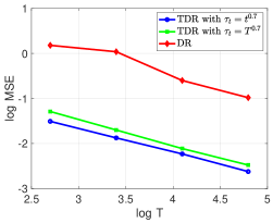
Figure 1: The $\log$ of $\mathsf{MSE}$ to the $\log$ of trajectory length $T$ for $\mathsf{TDR}$ and $\mathsf{DR}$ estimators under setup outlined in Example 1.

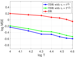
Figure 2: The $\log$ of $\mathsf{MSE}$ to the $\log$ of trajectory length $T$ for $\mathsf{TDR}$ and $\mathsf{DR}$ under setup given in Example 2 for truncation parameter $\delta=0.4$.

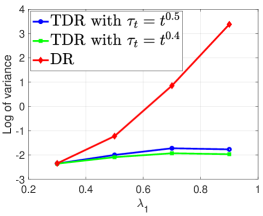
Figure 3: The $\log$ of variance to treatment arrival rate $\lambda_{1}$ for the random walk on non-negative integers setup outlined in Example 3.

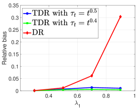
Figure 4: The relative bias value to treatment arrival rate $\lambda_{1}$ for the random walk on non-negative integers setup outlined in Example 3.

Example 3. In this experiment, we compare the empirical performance of $\mathsf{DR}$ and $\mathsf{TDR}$ estimators in terms of bias and variance. We adopt the similar setting given in Example 2, a random walk on non-negative integers. We set treatment probabilities under evaluation and behavior policies $q_{e}=1$ and $q_{b}=0.3$, respectively. In addition, we fix $\lambda_{0}=0.1$ and $\gamma=0.5$. We focus on estimating the discounted average reward $\theta_{\gamma}(p_{0})$, with the initial distribution being the stationary distribution under the evaluation policy.

We consider a range of values for $\lambda_{1}$, where it is selected from the set $\{0.3,0.5,0.7,0.9\}$. As we increase the values of $\lambda_{1}$, this leads to a shift towards states with larger values. Given that the probability of treatment is larger under the evaluation policy and the arrival rate $\lambda_{1}$ under treatment is much larger than the arrival rate $\lambda_{0}$ under control, this will drive the random walk to explore further states (larger integers values), compared to the MDP state visitation under the behavior policy. Thereby, as $\lambda_{1}$ increases, the strong distributional overlap assumption will be violated and result in extremely large values for $\omega(s)$.

We use estimate $\hat{\omega}=\omega$ for both estimators and for the estimate $\widehat{Q}(s,a)$, we use the discounted reward value obtained by averaging over $20000$ trajectories of length $20$ for starting state $s$ and action $a$. The same estimates are used for both estimators.

We use collected data under behavior policy of length $T=500$, and we employ the $\mathsf{TDR}$ estimator $\hat{\theta}_{\gamma}^{\mathsf{TDR}}(p_{0})$ with two truncation rates: $\tau_{t}=t^{0.4}$ and $\tau_{t}=t^{0.5}$. For each value of $\lambda_{1}$, we compute the off-policy outcomes for three estimators ($\mathsf{DR}$ and $\mathsf{TDR}$ with two truncation rates) and report the average bias and variance across $5000$ independent experiments. The logarithms of variances are depicted in Figure 4, and the relative biases are reported as $\frac{|{\hat{\theta}_{\gamma}^{\mathsf{TDR}}(p_{0})}-\theta_{\gamma}(p_{0})|}{\theta_{\gamma}(p_{0})}$ in Figure 4. It can be observed that as $\lambda_{1}$ increases and the strong distributional overlap is violated, the $\mathsf{DR}$ estimator exhibits poor performance in terms of both bias and variance. This is in contrast to $\mathsf{TDR}$, which even for large values of $\lambda_{1}$, has significantly smaller bias and variance. The similar behavior for both truncation rates of $\mathsf{TDR}$ implies robustness with respect to truncation rate values

Appendix A Background results

A.1 Proof of Lemma 2.1

First, note that we have

$$q_{e}^{\gamma}(s,a) ={\mathbb{E}}_{\pi_{e}}\left[\sum_{t=0}^{\infty}R_{t}\gamma^{t}|S_{0}=s,A_{0}=a\right]$$

$$={\mathbb{E}}[R_{0}|S_{0}=s,A_{0}=a]+\gamma{\mathbb{E}}\left[\sum_{t=1}^{\infty}R_{t}\gamma^{t-1}|S_{0}=s,A_{0}=a\right]$$

$$={\mathbb{E}}[R_{0}|S_{0}=s,S_{0}=a]+\gamma\int{\mathbb{E}}\left[\sum_{t=1}^{\infty}R_{t}\gamma^{t-1}\Big{|}S_{1}=s^{\prime}\right]p_{s}(s^{\prime}|s,a){\rm d}\lambda(s^{\prime})$$

$$={\mathbb{E}}[R_{0}|S_{0}=s,A_{0}=a]+\gamma\int v_{e}^{\gamma}(s^{\prime})p_{s}(s^{\prime}|s,a){\rm d}\lambda(s^{\prime})$$

$$={\mathbb{E}}[R_{0}|S_{0}=s,A_{0}=a]+\gamma{\mathbb{E}}[v_{e}^{\gamma}(S_{1})|S_{0}=s,A_{0}=a]\,.$$

This gives us

$${\mathbb{E}}[-q_{e}^{\gamma}(S_{0},A_{0})+R_{0}+\gamma v_{e}^{\gamma}(S_{1})|S_{0},A_{0}]=0\,.$$

This completes the proof. We next prove the result for the long-run differential value functions.

$$Q_{e}(s,a) ={\mathbb{E}}_{\pi_{e}}\left[\sum_{t=0}^{\infty}(R_{t}-\theta)\Big{|}S_{0}=s,A_{0}=a\right]$$

$$={\mathbb{E}}_{\pi_{e}}[R_{0}|S_{0}=s,A_{0}=a]-\theta+{\mathbb{E}}\left[\sum_{t=1}^{\infty}(R_{t}-\theta)\Big{|}S_{0}=s,A_{0}=a\right]$$

$$={\mathbb{E}}[R_{0}|S_{0}=s,A_{0}=a]-\theta+\int V_{e}(s^{\prime})p_{s}(s^{\prime}|s,a){\rm d}\lambda_{s}(s^{\prime})$$

$$={\mathbb{E}}[R_{0}|S_{0}=s,A_{0}=a]-\theta+\int V_{e}(s^{\prime})p_{s}(s^{\prime}|s,a){\rm d}\lambda_{s}(s^{\prime})\,.$$

This completes the proof.

A.2 Proof of Lemma 2.2

From the definition of the discounted average frequency visits $p^{\gamma}_{e}(.;p_{0})$ we have

$$p^{\gamma}_{e}(s^{\prime};p_{0}) =(1-\gamma)p_{0}(s^{\prime})+(1-\gamma)\gamma\sum_{t=1}^{\infty}\gamma^{t-1}{\mathbb{P}}_{\pi_{e}}(S_{t}=s^{\prime}|s_{0}\sim p_{0})\,.$$ (29)

Let $p_{\pi_{e}}(s^{\prime}|s)$ denote the marginal state transition under the evaluation policy $\pi_{e}$, specifically let

$$p_{\pi_{e}}(s^{\prime}|s)=\int p_{s}(s^{\prime}|s,a)\pi_{e}(a|s){\rm d}\lambda_{a}(a)\,.$$ (30)

Using this for $t\geq 1$ brings us

$${\mathbb{P}}_{\pi_{e}}(S_{t}=s^{\prime}|s_{0}\sim p_{0})=\int{\mathbb{P}}_{\pi_{e}}(S_{t-1}=s|s_{0}\sim p_{0})p_{\pi^{e}}(s^{\prime}|s){\rm d}\lambda_{s}(s)\,.$$ (31)

Employing (31) in (29) yields

$$p^{\gamma}_{e}(s^{\prime};p_{0}) =(1-\gamma)p_{0}(s^{\prime})+\gamma(1-\gamma)\sum_{t=1}^{\infty}\gamma^{t-1}\int{\mathbb{P}}_{\pi_{e}}(S_{t-1}=s|s_{0}\sim p_{0})p_{\pi^{e}}(s^{\prime}|s){\rm d}\lambda_{s}(s)$$

$$=(1-\gamma)p_{0}(s^{\prime})+\gamma\int\Big{(}p_{\pi^{e}}(s^{\prime}|s)\cdot(1-\gamma)\sum_{t=1}^{\infty}\gamma^{t-1}{\mathbb{P}}_{\pi_{e}}(S_{t-1}=s|s_{0}\sim p_{0})\Big{)}{\rm d}\lambda_{s}(s)$$

$$=(1-\gamma)p_{0}(s^{\prime})+\gamma\int p^{\gamma}_{e}(s;p_{0})p_{\pi^{e}}(s^{\prime}|s){\rm d}\lambda_{s}(s)\,,$$

where in the last relation we used the definition of $p^{\gamma}_{e}((;p_{0}).)$. In summary, the above gives us

$$p^{\gamma}_{e}(s^{\prime};p_{0})=(1-\gamma)p_{0}(s^{\prime})+\gamma\int p^{\gamma}_{e}(s;p_{0})p_{\pi^{e}}(s^{\prime}|s){\rm d}\lambda_{s}(s)\,.$$ (32)

In the next step, using $\omega^{\gamma}(s;p_{0})=\frac{p^{\gamma}_{e}(s;p_{0})}{p_{b}(s)}$ yields

$${\mathbb{E}}_{p_{b}}[f(S^{\prime})\omega^{\gamma}(S^{\prime};p_{0})] ={\mathbb{E}}_{p^{\gamma}_{e}(.;p_{0})}[f(S^{\prime})]$$

$$=\int f(s^{\prime})p^{\gamma}_{e}(s^{\prime};p_{0}){\rm d}\lambda_{s}(s^{\prime})\,.$$

Employing (32) in the above gives us

$${\mathbb{E}}_{p_{b}}[f(S^{\prime})\omega^{\gamma}(S^{\prime};p_{0})] =(1-\gamma)\int f(s^{\prime})p_{0}(s^{\prime}){\rm d}\lambda_{s}(s^{\prime})+\gamma\iint f(s^{\prime})p_{\pi_{e}}(s^{\prime}|s)p^{\gamma}_{e}(s;p_{0}){\rm d}\lambda_{s}(s){\rm d}\lambda_{s}(s^{\prime})\,.$$

We next use $p^{\gamma}_{e}(s;p_{0})=\omega^{\gamma}(s;p_{0})p_{b}(s)$ to get

$${\mathbb{E}}_{p_{b}}[f(S^{\prime})\omega(S^{\prime})] =(1-\gamma)\int f(s^{\prime})p_{0}(s^{\prime}){\rm d}\lambda_{s}(s^{\prime})+\gamma\iint f(s^{\prime})p_{\pi_{e}}(s^{\prime}|s)\omega^{\gamma}(s;p_{0})p_{b}(s){\rm d}\lambda_{s}(s){\rm d}\lambda_{s}(s^{\prime})$$

$$=(1-\gamma)\int f(s^{\prime})p_{0}(s^{\prime}){\rm d}\lambda_{s}(s^{\prime})\,$$

$$\,~{}+\gamma\iint f(s^{\prime})\Big{(}\int p_{s}(s^{\prime}|s,a)\pi_{e}(s|a){\rm d}\lambda_{a}(a)\Big{)}\omega^{\gamma}(s;p_{0})p_{b}(s){\rm d}\lambda_{s}(s){\rm d}\lambda_{s}(s^{\prime})\,,$$

where in the last relation we deployed (30). Finally, by using $\eta(s,a)=\frac{\pi_{e}(a|s)}{\pi_{b}(a|s)}$ we arrive at

$${\mathbb{E}}_{p_{b}}[f(S^{\prime})\omega^{\gamma}(S^{\prime};p_{0})] =(1-\gamma){\mathbb{E}}_{p_{0}}[f(S)]$$

$$+\gamma\iiint f(s^{\prime})\omega^{\gamma}(s;p_{0})\eta(s,a)p_{b}(s)p_{s}(s^{\prime}|s,a)\pi_{b}(a|s){\rm d}\lambda_{s}(s){\rm d}\lambda_{a}(a){\rm d}\lambda_{s}(s^{\prime})\,.$$

Put all together, we get

$${\mathbb{E}}_{p_{b}}[f(S)\omega^{\gamma}(S;p_{0})]=(1-\gamma){\mathbb{E}}_{p_{0}}[f(S)]+\gamma{\mathbb{E}}_{(S,A,S^{\prime})\sim p_{b}(S)\pi_{b}(A|S)p(S^{\prime}|S,A)}\left[\omega^{\gamma}(S;p_{0})\eta(S,A)f(S^{\prime})\right]\,.$$

This completes the proof.

We next move to the proof for the long-run density ratio function $\omega(s)$. Similar to the previous part, we let $\eta(s,a)=\frac{\pi_{e}(a|s)}{\pi_{b}(a|s)}$. We have

$${\mathbb{E}}[\omega(S)\eta(S,A)f(S^{\prime})] =\iiint\omega(S)\eta(S,A)f(S^{\prime})p_{b}(S)\pi_{b}(A|S)p_{s}(S^{\prime}|S,A){\rm d}\lambda_{a}(A){\rm d}\lambda_{s}(S){\rm d}\lambda_{s}(S^{\prime})\,.$$

We next use the definition for density ratio function $\omega(s)$ and $\eta(s,a)$ to arrive at

$${\mathbb{E}}[\omega(S)\eta(S,A)f(S^{\prime})] =\iiint f(s^{\prime})p_{e}(s)\pi_{e}(a|s)p_{s}(s^{\prime}|s,a){\rm d}\lambda_{a}(a){\rm d}\lambda_{s}(s){\rm d}\lambda_{s}(s^{\prime})$$

$$=\int f(s^{\prime})\left(\iint p_{e}(s)\pi_{e}(a|s)p_{s}(s^{\prime}|s,a){\rm d}\lambda_{a}(a){\rm d}\lambda_{s}(s)\right){\rm d}\lambda_{s}(s^{\prime})\,.$$

We next use the invariance of stationary state distribution $p_{e}$ under evaluation policy, which reads as

$$\iint p_{e}(s)\pi_{e}(a|s)p_{s}(s^{\prime}|s,a){\rm d}\lambda_{a}(a){\rm d}\lambda_{s}(s)=p_{e}(s^{\prime})\,.$$

Using this in the above yields

$${\mathbb{E}}[\omega(S)\eta(S,A)f(S^{\prime})] =\int f(s^{\prime})p_{e}(s^{\prime}){\rm d}\lambda_{s}(s^{\prime})$$

$$=\int f(s^{\prime})\omega(s^{\prime})p_{b}(s^{\prime}){\rm d}\lambda_{s}(s^{\prime})$$

$$={\mathbb{E}}_{p_{b}}[\omega(S)f(S)]\,.$$

This completes the proof.

Appendix B Preliminaries and technical lemmas

We let $\eta(s,a)=\frac{\pi_{e}(a|s)}{\pi_{b}(a|s)}$. For states $s,s^{\prime}\in\mathcal{S}$, an action $a\in\mathcal{A}$, reward value $r\in{\mathcal{R}}$, and functions $f_{\omega}:\mathcal{S}\to{\mathbb{R}}$, $f_{q}:\mathcal{S}\times\mathcal{A}\to{\mathbb{R}}$, and $f_{v}(S)={\mathbb{E}}_{\pi_{e}}[f_{q}(S,A)|S]$ we let $\psi(s,a,r,s^{\prime};f_{\omega},f_{q})$ represents the following

$$\psi(s,a,r,s^{\prime};f_{\omega},f_{q})=(1-\gamma){\mathbb{E}}_{S_{0}\sim p_{0}}\left[f_{v}(S_{0})\right]+f_{\omega}(s)\eta(s,a)(r+\gamma f_{v}(s^{\prime})-f_{q}(s,a))\,.$$

For the tuple $(S_{t},A_{t},R_{t},S_{t+1})$, we introduce the following shorthand:

$$\psi_{t}=\psi\left(S_{t},A_{t},R_{t},S_{t+1};\omega^{\gamma}(.;p_{0}),q_{e}^{\gamma}\right)\,.$$

We also let ${\hat{\omega}}_{t}=\hat{\omega}^{\gamma}(S_{t};p_{0})$ (for the discounted estimation problem) or ${\hat{\omega}}_{t}=\hat{\omega}(S_{t})$ (for the long-run average estimation problem), $\eta_{t}=\eta(S_{t},A_{t})$, $\hat{q}^{\gamma}_{t}=\hat{q}^{\gamma}_{e}(S_{t})$ and $\hat{v}^{\gamma}_{t}=v^{\gamma}_{e}(S_{t})$. In addition, for model estimates $\hat{\omega}^{\gamma}(.;p_{0})$ and $\hat{q}^{\gamma}_{e}$ we let

$$\widehat{\psi}_{t}=\psi\Big{(}S_{t},A_{t},R_{t},S_{t+1};\hat{\omega}^{\gamma}(.;p_{0}),\hat{q}_{e}^{\gamma}\Big{)}\,.$$

It is easy to observe that the $\mathsf{DR}$ estimator for the discounted average reward can be written as the following:

$$\hat{\theta}_{\gamma}^{\mathsf{DR}}(p_{0}) =\frac{1}{T}\sum\limits_{t=1}^{T}\widehat{\psi}_{t}\,.$$

Similar to discussed above, for the long-run model estimates $\widehat{Q}_{e}$ and $\widehat{V}_{e}$, we also let $V_{t}=V_{e}(S_{t})$, $\widehat{V}_{t}=\widehat{V}_{e}(S_{t})$, $Q_{t}=Q_{e}(S_{t},A_{t})$, and $\widehat{Q}_{t}=\widehat{Q}_{e}(S_{t},A_{t})$. In addition, for the long-run average reward $\theta$ estimation problem, we adopt the following shorthands:

$$c_{t} =\omega_{t}\eta_{t}\,,$$

$$\widehat{c}_{t} =\hat{\omega}_{t}\eta_{t}\,,$$

$$b_{t} =(R_{t}+V_{t+1}-Q_{t}-\theta)\,,$$

$$\widehat{b}_{t} =(R_{t}+\widehat{V}_{t+1}-\widehat{Q}_{t}-\theta)\,.$$ (33)

We end this section by stating lemmas that we will use later in the proof of Theorems.

Lemma B.1.

Under Assumptions 1-5, and $\gamma$-discounted $\delta$-weak distributional overlap for some $\delta>1$, suppose that estimates $\hat{q}^{\gamma}_{e}(.)$ and ${\hat{\omega}}^{\gamma}(.;p_{0})$ satisfy Assumption 6, and equation (17) for parameters $\kappa_{T},\xi_{T},$ and $\mu_{T}$ such that $\kappa_{T}\vee\xi_{T}\vee\mu_{T}=o_{T}(1)$. Then the following holds

$$\sqrt{T}\Big{(}\frac{1}{T}\sum_{t=1}^{T}(\widehat{\psi}_{t}-\psi_{t})-\big{(}\hat{\theta}^{\mathsf{DR}}_{\gamma}(p_{0})-\theta_{\gamma}(p_{0})\big{)}\Big{)}=o_{T}(1)\,.$$

The proof of this Lemma can be seen in Section B.1.

Lemma B.2 (Doubly robustness).

Under Assumptions 1-5, for estimates $\hat{q}^{\gamma}_{e}(.)$ and ${\hat{\omega}}^{\gamma}(.;p_{0})$ satisfying Assumption 6 with parameters $\kappa_{T}$ and $\xi_{T}$, we have

$$\left|\hat{\theta}_{\gamma}^{\mathsf{DR}}(p_{0})-\theta_{\gamma}(p_{0})\right|\lesssim\kappa_{T}\xi_{T}\,.$$

We refer to Section B.2 for the proof of Lemma B.2.

Lemma B.3.

We consider the off-policy evaluation problem under Assumptions 1-5, geometric mixing assumption 7, and the long-run $\delta$-weak distributional overlap condition for $\delta>1$. In addition, we suppose that estimates $\widehat{Q}_{e}$ and ${\hat{\omega}}$ satisfy Assumption 8 and equation (21) for parameters $\Xi_{T},K_{T}$, and $M_{T}$ such that $\Xi_{T}\vee M_{T}=o_{T}(1)$. Then we have

$$\frac{1}{\sqrt{T}}\sum_{t=1}^{T}\left(\widehat{c}_{t}\widehat{b}_{t}-c_{t}b_{t}-{\mathbb{E}}[\widehat{c}_{t}\widehat{b}_{t}]+{\mathbb{E}}[c_{t}b_{t}]\right)=o_{T}(1)\,.$$

The proof of this Lemma can be seen in Section B.3.

Lemma B.4.

Under Assumptions 1-5, for estimates $\widehat{Q}_{e},\hat{\omega}$ satisfying Assumption 8 with parameters $K_{T}$ and $\Xi_{T}$, we have ${\mathbb{E}}[c_{t}b_{t}]=0$, and also the following holds

$$\left|{\mathbb{E}}[\widehat{c}_{t}\widehat{b}_{t}]\right|\leq C_{\eta}K_{T}\Xi_{T}\,,$$

where $C_{\eta}$ is the policy overlap parameter given in Assumption 3.

We refer to Section B.4 for the proof of Lemma B.4.

B.1 Proof of Lemma B.1

By using the identity $(\widehat{a}\widehat{b}-ab)=(\widehat{a}-a)(\widehat{b}-b)+a(\widehat{b}-b)+(\widehat{a}-a)b$ we get

$$\widehat{\psi}_{t}-\psi_{t} =\eta_{t}({\hat{\omega}}_{t}-\omega_{t})(\gamma\hat{v}^{\gamma}_{t+1}-\gamma v_{t+1}+q_{t}-\hat{q}^{\gamma}_{t})+(1-\gamma){\mathbb{E}}_{p_{0}}[\hat{v}^{\gamma}_{e}(S)-v^{\gamma}_{e}(S)]$$

$$~{}\,+\eta_{t}\omega_{t}(q_{t}-\gamma v_{t+1}-\hat{q}^{\gamma}_{t}+\gamma\hat{v}^{\gamma}_{t+1})+\eta_{t}({\hat{\omega}}_{t}-\omega_{t})(R_{t}+\gamma v_{t+1}-q_{t})\,.$$

In the next step, using ${\rm Var}(\widehat{\psi}_{t}-\psi_{t})\leq{\mathbb{E}}[(\widehat{\psi}_{t}-\psi_{t})^{2}]$ in conjunction with Cauchy-Schwartz inequality we arrive at

$${\rm Var}(\widehat{\psi}_{t}-\psi_{t}) \leq 4{\mathbb{E}}[\eta_{t}^{2}({\hat{\omega}}_{t}-\omega_{t})^{2}(\gamma\hat{v}^{\gamma}_{t+1}-\gamma v_{t+1}+q_{t}-\hat{q}^{\gamma}_{t})^{2}]+4(1-\gamma)^{2}{\mathbb{E}}_{p_{0}}[(\hat{v}^{\gamma}_{e}(S)-v_{e}^{\gamma}(S))^{2}]$$

$$~{}\,+4{\mathbb{E}}[\eta_{t}^{2}\omega_{t}^{2}(q_{t}-\gamma v_{t+1}-\hat{q}^{\gamma}_{t}+\gamma\hat{v}^{\gamma}_{t+1})^{2}]+4{\mathbb{E}}[\eta_{t}^{2}({\hat{\omega}}_{t}-\omega_{t})^{2}(R_{t}+\gamma v_{t+1}-q_{t})^{2}]\,.$$

We next deploy $\eta_{t}\leq C_{\eta}$ (policy overlap assumption) and $\max(\hat{v}^{\gamma}_{e},v_{e}^{\gamma},q_{e}^{\gamma},\hat{q}^{\gamma}_{e})\leq\frac{1}{1-\gamma}R_{\max}$ to get

$${\rm Var}(\widehat{\psi}_{t}-\psi_{t}) \lesssim{\mathbb{E}}_{p_{b}}\left[\|{\hat{\omega}}^{\gamma}(S;p_{0})-\omega^{\gamma}(S;p_{0})\|_{2}^{2}\right]+{\mathbb{E}}_{p_{0}}\left[\|\hat{v}^{\gamma}_{e}(S)-v_{e}^{\gamma}(S)\|_{2}^{2}\right]$$

$$\,+{\mathbb{E}}_{p_{b}}\left[\omega(S)^{2}\|\hat{q}^{\gamma}_{e}(S)-q_{e}^{\gamma}(S)\|_{2}^{2}\right]+{\mathbb{E}}_{p_{b}}\left[\|{\hat{\omega}}^{\gamma}(S;p_{0})-\omega^{\gamma}(S;p_{0})\|_{2}^{2}\right]\,.$$

We then use Holder’s inequality ${\mathbb{E}}[|xy|]\leq{\mathbb{E}}[|x|^{p}]^{\frac{1}{p}}{\mathbb{E}}[|x|^{q}]^{\frac{1}{q}}$ for $p=\frac{1+\delta}{2}$ and $q=\frac{1+\delta}{\delta-1}$. This yields

$${\rm Var}(\widehat{\psi}_{t}-\psi_{t}) \lesssim{\mathbb{E}}_{p_{b}}\left[\|{\hat{\omega}}^{\gamma}(S)-\omega^{\gamma}(S)\|_{2}^{2}\right]+{\mathbb{E}}_{p_{0}}\left[\|\hat{v}^{\gamma}_{e}(S)-v_{e}^{\gamma}(S)\|_{2}^{2}\right]$$

$$\,+{\mathbb{E}}_{p_{b}}\left[\omega^{\gamma}(S;p_{0})^{1+\delta}\right]^{\frac{2}{1+\delta}}{\mathbb{E}}\left[\|\hat{q}^{\gamma}_{e}(S)-q_{e}^{\gamma}(S)\|_{2}^{\frac{2(1+\delta)}{\delta-1}}\right]^{\frac{\delta-1}{\delta+1}}\,.$$

Finally, employing the $\gamma$-discounted $\delta$-weak distributional overlap condition in along with estimates Assumption 6 and equation (17) yields

$${\rm Var}(\widehat{\psi}_{t}-\psi_{t})=O\left(\kappa_{T}^{2}\vee\xi_{T}^{2}\vee\mu_{T}^{2}\right)\,.$$ (34)

In the next step, we have

$${\rm Var}\left(\sqrt{T}\Big{(}\frac{1}{T}\sum_{t=1}^{T}(\widehat{\psi}_{t}-\psi_{t})\Big{)}\right) =\frac{1}{T}\sum_{t=1}^{T}{\rm Var}(\widehat{\psi}_{t}-\psi_{t})+\frac{1}{T}\sum_{\ell\neq k}^{T}{\rm Cov}(\widehat{\psi}_{k}-\psi_{k},\widehat{\psi}_{\ell}-\psi_{\ell})$$

$$={\rm Var}(\psi_{1}-\widehat{\psi}_{1})+\frac{{\rm Var}(\psi_{1}-\widehat{\psi}_{1})}{T}\sum_{\ell\neq k}^{T}{\rm corr}(\widehat{\psi}_{k}-\psi_{k},\widehat{\psi}_{\ell}-\psi_{\ell}))$$

$$\leq{\rm Var}(\psi_{1}-\widehat{\psi}_{1})\left(1+\frac{2}{T}\sum_{\ell<k}^{T}\rho_{k-\ell}\right)\,,$$

where in the last relation we used the definition of $\rho_{n}$ mixing. Finally, using Assumption 4 that $\sum\rho_{n}<+\infty$ in along with (34) yields

$${\rm Var}\left(\sqrt{T}\Big{(}\frac{1}{T}\sum_{t=1}^{T}(\widehat{\psi}_{t}-\psi_{t})\Big{)}\right)=O\left(\kappa_{T}^{2}\vee\xi_{T}^{2}\vee\mu_{T}^{2}\right)\,.$$

Given that ${\mathbb{E}}[(\widehat{\psi}_{t}-\psi_{t})]=\widehat{\theta}_{\gamma}^{\mathsf{DR}}(p_{0})-\theta_{\gamma}(p_{0})$, by an application of Chebyshev’s inequality we get for every ${\varepsilon}>0$ we have

$$\lim_{T\to\infty}{\mathbb{P}}\left(\sqrt{T}\Big{(}\frac{1}{T}\sum_{t=1}^{T}(\widehat{\psi}_{t}-\psi_{t})-(\widehat{\theta}_{\gamma}^{\mathsf{DR}}(p_{0})-\theta_{\gamma}(p_{0}))\Big{)}\geq{\varepsilon}\right)\leq\lim_{T\to\infty}\frac{O\left(\kappa_{T}^{2}\vee\xi_{T}^{2}\vee\mu_{T}^{2}\right)}{{\varepsilon}^{2}}=0\,,$$

where we used the fact that $\kappa_{t}\vee\xi_{T}\vee\mu_{T}=o_{T}(1)$. This completes the proof that $\sqrt{T}\Big{(}\frac{1}{T}\sum_{t=1}^{T}(\widehat{\psi}_{t}-\psi_{t})-(\widehat{\theta}_{\gamma}^{\mathsf{DR}}(p_{0})-\theta_{\gamma}(p_{0}))\Big{)}=o_{T}(1)$.

B.2 Proof of Lemma B.2

By using the identity $(\widehat{a}\widehat{b}-ab)=(\widehat{a}-a)(\widehat{b}-b)+a(\widehat{b}-b)+(\widehat{a}-a)b$ we get

$$\widehat{\psi}_{t}-\psi_{t} =\eta_{t}({\hat{\omega}}_{t}-\omega_{t})(\gamma\hat{v}^{\gamma}_{t+1}-\gamma v_{t+1}+q_{t}-\hat{q}^{\gamma}_{t})+(1-\gamma){\mathbb{E}}_{p_{0}}[\hat{v}^{\gamma}_{e}(S)-v^{\gamma}_{e}(S)]$$

$$~{}\,+\eta_{t}\omega_{t}(q_{t}-\gamma v_{t+1}-\hat{q}^{\gamma}_{t}+\gamma\hat{v}^{\gamma}_{t+1})+\eta_{t}({\hat{\omega}}_{t}-\omega_{t})(R_{t}+\gamma v_{t+1}-q_{t})\,.$$

This gives us

$$\hat{\theta}^{\mathsf{DR}}_{\gamma}(p_{0})-\theta_{\gamma}(p_{0}) =\frac{1}{{T}}{\mathbb{E}}\left[\sum_{t=1}^{T}(\widehat{\psi}_{t}-\psi_{t})\right]$$

$$=\frac{1}{{T}}\sum_{t=1}^{T}{\mathbb{E}}\left[\eta_{t}({\hat{\omega}}_{t}-\omega_{t})(\gamma\hat{v}^{\gamma}_{t+1}-\gamma v_{t+1}+q_{t}-\hat{q}^{\gamma}_{t})+(1-\gamma){\mathbb{E}}_{p_{0}}[\hat{v}^{\gamma}_{e}(S)-v^{\gamma}_{e}(S)]\right]$$

$$~{}\,+\frac{1}{{T}}\sum_{t=1}^{T}{\mathbb{E}}\left[\eta_{t}\omega_{t}(q_{t}-\gamma v_{t+1}-\hat{q}^{\gamma}_{t}+\gamma\hat{v}^{\gamma}_{t+1})+\eta_{t}({\hat{\omega}}_{t}-\omega_{t})(R_{t}+\gamma v_{t+1}-q_{t})\right]\,.$$ (35)

By using Jensen’s inequality we obtain

$${\mathbb{E}}\left[({\hat{\omega}}_{t}-\omega_{t})(\gamma\hat{v}^{\gamma}_{t+1}-\gamma v_{t+1}+q_{t}-\hat{q}^{\gamma}_{t})\right] \leq{\mathbb{E}}\left[({\hat{\omega}}_{t}-\omega_{t})^{2}\right]^{1/2}{\mathbb{E}}\left[(\gamma\hat{v}^{\gamma}_{t+1}-\gamma v_{t+1}+q_{t}-\hat{q}^{\gamma}_{t})^{2}\right]^{1/2}$$

$$\lesssim\kappa_{T}\xi_{T}\,.$$

Using this in (35) yields

$$\Big{|}\hat{\theta}^{\mathsf{DR}}_{\gamma}(p_{0})-\theta_{\gamma}(p_{0})\Big{|} \lesssim\kappa_{T}\xi_{T}+\Big{|}\frac{1}{{T}}\sum_{t=1}^{T}\left({\mathbb{E}}[\eta_{t}\omega_{t}(q_{t}-\gamma v_{t+1}-\hat{q}^{\gamma}_{t}+\gamma\hat{v}^{\gamma}_{t+1})]+(1-\gamma){\mathbb{E}}_{p_{0}}[\hat{v}^{\gamma}_{e}(S)-v_{e}^{\gamma}(S)]\right)\Big{|}$$

$$\,+\Big{|}\frac{1}{{T}}\sum_{t=1}^{T}{\mathbb{E}}[\eta_{t}({\hat{\omega}}_{t}-\omega_{t})(R_{t}+\gamma v_{t+1}-q_{t})]\Big{|}\,.$$ (36)

In the next step, we deploy Lemma 2.1 to get

$${\mathbb{E}}[\eta_{t}({\hat{\omega}}_{t}-\omega_{t})(R_{t}+\gamma v_{t+1}-q_{t})]={\mathbb{E}}[\eta_{t}({\hat{\omega}}_{t}-\omega_{t}){\mathbb{E}}[(R_{t}+\gamma v_{t+1}-q_{t})|S_{t},A_{t}]]=0\,.$$

By employing this in (36) we obtain

$$|\hat{\theta}^{\mathsf{DR}}_{\gamma}(p_{0})-\theta_{\gamma}(p_{0})|\lesssim\kappa_{T}\xi_{T}+\Big{|}\frac{1}{{T}}\sum_{t=1}^{T}\left({\mathbb{E}}[\eta_{t}\omega_{t}(q_{t}-\gamma v_{t+1}-\hat{q}^{\gamma}_{t}+\gamma\hat{v}^{\gamma}_{t+1})]+(1-\gamma){\mathbb{E}}_{p_{0}}[\hat{v}^{\gamma}(S)-v(S)]\right)\Big{|}$$ (37)

We next use Lemma 2.2 with the measurable function $f(s)=-v_{e}^{\gamma}(s)+\hat{v}^{\gamma}_{e}(s)$ to get

$$\gamma{\mathbb{E}}[\eta_{t}\omega_{t}(-v_{t+1}+\hat{v}^{\gamma}_{t+1})]+(1-\gamma){\mathbb{E}}_{p_{0}}[\hat{v}^{\gamma}_{e}(S)-v_{e}^{\gamma}(S)]={\mathbb{E}}[\omega_{t}(\hat{v}^{\gamma}_{t}-v_{t})]\,.$$ (38)

In addition, we have

$${\mathbb{E}}[\eta_{t}\omega_{t}(q_{t}-\hat{q}^{\gamma}_{t})] ={\mathbb{E}}[{\mathbb{E}}[\eta_{t}\omega_{t}(q_{t}-\hat{q}^{\gamma}_{t})|S_{t}]]$$

$$={\mathbb{E}}[\omega_{t}{\mathbb{E}}_{\pi^{e}}[q_{t}-\hat{q}^{\gamma}_{t}|S_{t}]]$$

$$={\mathbb{E}}[\omega_{t}(v_{t}-\hat{v}^{\gamma}_{t})]\,.$$ (39)

Combining (39) and (38) brings us

$${\mathbb{E}}[\eta_{t}\omega_{t}(q_{t}-\gamma v_{t+1}-\hat{q}^{\gamma}_{t}+\gamma\hat{v}^{\gamma}_{t+1})]+(1-\gamma){\mathbb{E}}_{p_{0}}[\hat{v}^{\gamma}_{e}(S)-v_{e}^{\gamma}(S)]=0\,.$$

Plugging this into (37) yields

$$|\hat{\theta}^{\mathsf{DR}}_{\gamma}(p_{0})-\theta_{\gamma}(p_{0})|\lesssim\kappa_{T}\xi_{T}\,.$$

B.3 Proof of Lemma B.3

Following shorthands given in (33) we obtain

$${\rm Var}(\widehat{c}_{t}\widehat{b}_{t}-c_{t}b_{t})\leq 3{\mathbb{E}}\left[c_{t}^{2}(\widehat{b}_{t}-b_{t})^{2}\right]+3{\mathbb{E}}\left[(\widehat{c}_{t}-c_{t})^{2}b_{t}^{2}\right]+3{\mathbb{E}}\left[(\widehat{c}_{t}-c_{t})^{2}(\widehat{b}_{t}-b_{t})^{2}\right]\,.$$

This gives us

$${\rm Var}(\widehat{c}_{t}\widehat{b}_{t}-c_{t}b_{t})\lesssim{\mathbb{E}}\left[\omega(S)^{2}(\widehat{Q}(S,A)-Q(S,A))^{2}\right]+{\mathbb{E}}_{p_{b}}\left[(\hat{\omega}(S)-\omega(S))^{2}\right]\,.$$

We then use Holder’s inequality ${\mathbb{E}}[|X||Y|]\leq{\mathbb{E}}[|X|^{p}]^{\frac{1}{p}}{\mathbb{E}}[|Y|^{q}]^{\frac{1}{q}}$ for $p=\frac{1+\delta}{2}$ and $q=\frac{\delta+1}{\delta-1}$. This yields

$${\rm Var}(\widehat{c}_{t}\widehat{b}_{t}-c_{t}b_{t}) \lesssim{\mathbb{E}}_{p_{b}}\left[\|\omega-\hat{\omega}\|_{2}^{2}\right]+{\mathbb{E}}_{p_{b}}\left[\omega(S)^{1+\delta}\right]^{\frac{2}{1+\delta}}{\mathbb{E}}_{p_{b}}\left[\|\widehat{Q}-Q\|_{2}^{\frac{2(\delta+1)}{\delta-1}}\right]^{\frac{\delta-1}{(\delta+1)}}\,.$$

Finally, employing the $\delta$-weak distributional overlap for $\delta>1$ gives us that ${\mathbb{E}}_{p_{b}}[\omega(S)^{1+\delta}]$ is bounded. This in conjunction with Assumption 8 and equation (21) brings us

$${\rm Var}(\widehat{c}_{t}\widehat{b}_{t}-c_{t}b_{t})=O\left(M_{T}^{2}\vee\Xi_{T}^{2}\right)\,.$$ (40)

In the next step, we have

$${\rm Var}\left(\frac{1}{\sqrt{T}}\sum_{t=1}^{T}(\widehat{c}_{t}\widehat{b}_{t}-c_{t}b_{t})\right) =\frac{1}{T}\sum_{t=1}^{T}{\rm Var}(\widehat{c}_{t}\widehat{b}_{t}-c_{t}b_{t})+\frac{1}{T}\sum_{\ell\neq k}^{T}{\rm Cov}(\widehat{c}_{k}\widehat{b}_{k}-c_{k}b_{k},\widehat{c}_{\ell}\widehat{b}_{\ell}-c_{\ell}b_{\ell})$$

$$={\rm Var}(\widehat{c}_{1}\widehat{b}_{1}-c_{1}b_{1})+\frac{{\rm Var}(\widehat{c}_{1}\widehat{b}_{1}-c_{1}b_{1})}{T}\sum_{\ell\neq k}^{T}{\rm corr}(\widehat{c}_{k}\widehat{b}_{k}-c_{k}b_{k},\widehat{c}_{\ell}\widehat{b}_{\ell}-c_{\ell}b_{\ell})$$

$$\leq{\rm Var}(\widehat{c}_{1}\widehat{b}_{1}-c_{1}b_{1})\left(1+2\sum_{\ell=1}^{T}\rho_{\ell}\right)\,,$$

where in the last relation we used the definition of $\rho_{n}$-mixing coefficients. Using Assumption 4 that $\sum\rho_{n}\leq C_{\rho}$ in along with (40) yields

$${\rm Var}\left(\frac{1}{\sqrt{T}}\sum_{t=1}^{T}(\widehat{c}_{t}\widehat{b}_{t}-c_{t}b_{t})\right)=O\left(M_{T}^{2}\vee\Xi_{T}^{2}\right)\,.$$

Finally, by an application of Chebyshev’s inequality we obtain that for every ${\varepsilon}>0$ we must have

$$\lim_{T\to\infty}{\mathbb{P}}\left(\frac{1}{\sqrt{T}}\sum_{t=1}^{T}\Big{(}\widehat{c}_{t}\widehat{b}_{t}-c_{t}b_{t}-{\mathbb{E}}[\widehat{c}_{t}\widehat{b}_{t}]+{\mathbb{E}}[c_{t}b_{t}]\Big{)}\geq{\varepsilon}\right) \leq\lim_{T\to\infty}\frac{{\rm Var}\left(\frac{1}{\sqrt{T}}\sum_{t=1}^{T}(\widehat{c}_{t}\widehat{b}_{t}-c_{t}b_{t})\right)}{{\varepsilon}^{2}}$$

$$=\lim_{T\to\infty}\frac{O(M_{T}^{2}\vee\Xi_{T}^{2})}{{\varepsilon}^{2}}=0\,,$$

where we used the assumption that $M_{t}\vee\Xi_{T}=o_{T}(1)$. Put all together, this shows the following

$$\frac{1}{\sqrt{T}}\sum_{t=1}^{T}\Big{(}\widehat{c}_{t}\widehat{b}_{t}-c_{t}b_{t}-{\mathbb{E}}[\widehat{c}_{t}\widehat{b}_{t}]+{\mathbb{E}}[c_{t}b_{t}]\Big{)}=o_{T}(1)\,.$$

B.4 Proof of Lemma B.4

We recall definitions of $c_{t},b_{t},\widehat{c}_{t}$, and $\widehat{b}_{t}$:

$$c_{t}=\omega_{t}\eta_{t},\quad\widehat{c}_{t}=\hat{\omega}_{t}\eta_{t}\,,\quad b_{t}=(R_{t}+Q_{t}-V_{t+1}-\theta)\,,\quad\widehat{b}_{t}=(R_{t}+\widehat{Q}_{t}-\widehat{V}_{t+1}-\theta)\,.$$

We first note that

$${\mathbb{E}}\left[\omega_{t}\eta_{t}(R_{t}+V_{t+1}-Q_{t})\right] ={\mathbb{E}}\left[\omega_{t}\eta_{t}{\mathbb{E}}[(R_{t}+V_{t+1}-Q_{t})|S_{t},A_{t}]\right]$$

$$={\mathbb{E}}\left[\omega_{t}\eta_{t}\right]\theta\,.$$

where the second equations follows Lemma 2.1 for the long-run density ratio function $\omega(.)$. This implies that ${\mathbb{E}}[c_{t}b_{t}]=0$. We next use the identity $(\widehat{c_{t}}\widehat{b_{t}}-c_{t}b_{t})=(\widehat{c_{t}}-c_{t})(\widehat{b_{t}}-b_{t})+c_{t}(\widehat{b_{t}}-b_{t})+(\widehat{c_{t}}-c_{t})b_{t}$, using this brings us

$${\mathbb{E}}[\widehat{c}_{t}\widehat{b}_{t}] ={\mathbb{E}}[\widehat{c}_{t}\widehat{b}_{t}-c_{t}b_{t}]$$

$$=\frac{1}{T}\sum_{t=1}^{T}{\mathbb{E}}\left[\eta_{t}({\hat{\omega}}_{t}-\omega_{t})(\widehat{V}_{t+1}-V_{t+1}+Q_{t}-\widehat{Q}_{t})\right]$$ (41)

$$~{}\,+\frac{1}{T}\sum_{t=1}^{T}{\mathbb{E}}\left[\eta_{t}\omega_{t}(Q_{t}-V_{t+1}-\widehat{Q}_{t}+\widehat{V}_{t+1})\right]$$ (42)

$$~{}\,+\frac{1}{T}\sum_{t=1}^{T}{\mathbb{E}}[\eta_{t}(\hat{\omega}_{t}-\omega_{t})(R_{t}+V_{t+1}-Q_{t}-\theta)]\,.$$ (43)

We start with expression (41), by an application of Jensen’s inequality and policy overlap assumption we obtain

$${\mathbb{E}}\left[\eta_{t}(\hat{\omega}_{t}-\omega_{t})(\widehat{V}_{t+1}-V_{t+1}+Q_{t}-\widehat{Q}_{t})\right] \leq C_{\eta}{\mathbb{E}}\Big{[}(\hat{\omega}_{t}-\omega_{t})^{2}\Big{]}^{\frac{1}{2}}{\mathbb{E}}\Big{[}(\widehat{V}_{t+1}-V_{t+1}+Q_{t}-\widehat{Q}_{t})^{2}\Big{]}^{\frac{1}{2}}$$

$$\leq C_{\eta}K_{T}\Xi_{T}\,,$$ (44)

where in the last relation we used Assumption 8. For the term (42), we have

$${\mathbb{E}}\left[\eta_{t}\omega_{t}(Q_{t}-V_{t+1}-\widehat{Q}_{t}+\widehat{V}_{t+1})\right] ={\mathbb{E}}\left[\eta_{t}\omega_{t}(Q_{t}-\widehat{Q}_{t})\right]+{\mathbb{E}}\left[\eta_{t}\omega_{t}(-V_{t+1}+\widehat{V}_{t+1})\right]$$

$$={\mathbb{E}}\left[\eta_{t}\omega_{t}(Q_{t}-\widehat{Q}_{t})\right]+{\mathbb{E}}\left[\omega_{t}(-V_{t}+\widehat{V}_{t})\right]$$

$$={\mathbb{E}}\left[\omega_{t}(V_{t}-\widehat{V}_{t})\right]+{\mathbb{E}}\left[\omega_{t}(-V_{t}+\widehat{V}_{t})\right]=0\,,$$ (45)

where we used Lemma 2.2 for density ratio function $\omega(.)$. Finally, we focus on (43) to obtain

$${\mathbb{E}}[\eta_{t}(\hat{\omega}_{t}-\omega_{t})(R_{t}+V_{t+1}-Q_{t}-\theta)] ={\mathbb{E}}[\eta_{t}(\hat{\omega}_{t}-\omega_{t}){\mathbb{E}}[(R_{t}+V_{t+1}-Q_{t}-\theta)|S_{t},A_{t}]]$$

$$=0\,,$$ (46)

where we used Lemma 2.1 for $\omega(.)$. By combining (44), (45), and (46) we arrive at

$$\left|{\mathbb{E}}[\widehat{c}_{t}\widehat{b}_{t}]\right|\leq C_{\eta}K_{T}\Xi_{T}\,.$$ (47)

Appendix C Proof of Lemma 3.2

We let $\eta(s,a)=\frac{\pi_{e}(s,a)}{\pi_{b}(s,a)}$, and ${\hat{\omega}}_{t}=\hat{\omega}^{\gamma}(S_{t};p_{0})$ (for the discounted estimation problem), $\eta_{t}=\eta(S_{t},A_{t})$, $\hat{q}^{\gamma}_{t}=\hat{q}^{\gamma}_{e}(S_{t})$ and $\hat{v}^{\gamma}_{t}=\hat{v}^{\gamma}_{e}(S_{t})$. Similarly, $v_{t}=v^{\gamma}_{r}(S_{t})$, and $q_{t}=q^{\gamma}_{e}(S_{t})$. We first show that for $\delta\leq 1$, given the finite value of ${\mathbb{E}}_{p_{b}}[\|{\hat{\omega}}^{\gamma}(S;p_{0})-\omega^{\gamma}(S;p_{0})\|_{2}^{2}]$, the same tail inequality as in the weak distributional overlap can be established for ${\hat{\omega}}^{\gamma}(.;p_{0})$. In particular, using the triangle’s inequality we have

$${\mathbb{P}}_{p_{b}}\left({\hat{\omega}}^{\gamma}(S;p_{0})^{1+\delta}\geq x\right) ={\mathbb{P}}_{p_{b}}\left({\hat{\omega}}^{\gamma}(S;p_{0})\geq x^{\frac{1}{1+\delta}}\right)$$

$$\leq{\mathbb{P}}_{p_{b}}\left(\omega^{\gamma}(S;p_{0})\geq\frac{x^{\frac{1}{1+\delta}}}{2}\right)+{\mathbb{P}}_{p_{b}}\left(\Big{|}{\hat{\omega}}^{\gamma}(S;p_{0})-\omega^{\gamma}(S;p_{0})\Big{|}\geq\frac{x^{\frac{1}{1+\delta}}}{2}\right)\,.$$

We next use the $\delta$-weak distributional overlap assumption in along with Markov’s inequality to obtain

$${\mathbb{P}}_{p_{b}}\left({\hat{\omega}}^{\gamma}(S;p_{0})^{1+\delta}\geq x\right) \leq\frac{C2^{1+\delta}}{x}+\frac{2^{1+\delta}{\mathbb{E}}\left[|{\hat{\omega}}^{\gamma}(S;p_{0})-\omega^{\gamma}(S;p_{0})|^{1+\delta}\right]}{x}\,.$$

Given that we are in the setting of $\delta\leq 1$, from Assumption 6 we have ${\mathbb{E}}\left[|{\hat{\omega}}^{\gamma}(S;p_{0})-\omega^{\gamma}(S;p_{0})|^{2}\right]<+\infty$, therefore ${\mathbb{E}}\left[|{\hat{\omega}}^{\gamma}(S;p_{0})-\omega^{\gamma}(S;p_{0})|^{1+\delta}\right]<+\infty$. Using this in the above implies that there exists constant $C^{\prime}$ with finite value such that

$${\mathbb{P}}_{p_{b}}\left({\hat{\omega}}^{\gamma}(S;p_{0})^{1+\delta}\geq x\right)\leq\frac{C^{\prime}}{x}\,.$$ (48)

Let $\lambda_{t}=\eta_{t}(\hat{\omega}_{t}\wedge\tau_{t})(R_{t}+\gamma\hat{v}_{t+1}-\hat{q}_{t})$. For the variance term, we have

$${\rm Var}({\hat{\theta}}^{\mathsf{TDR}}_{e}) ={\rm Var}\left(\frac{1}{T}\sum_{t=1}^{T}\lambda_{t}\right)$$

$$=\frac{1}{T^{2}}\sum_{t=1}^{T}{\rm Var}(\lambda_{t})+\frac{2}{T^{2}}\sum\limits_{1\leq\ell<t\leq T}{\rm Cov}(\lambda_{\ell},\lambda_{t})$$

$$=\frac{1}{T^{2}}\sum_{t=1}^{T}{\rm Var}(\lambda_{t})+\frac{2}{T^{2}}\sum\limits_{\ell<t}{{\rm corr}(\lambda_{\ell},\lambda_{t})}{{\rm Var}(\lambda_{\ell})^{1/2}{\rm Var}(\lambda_{t})^{1/2}}\,,$$

where in the last relation we used the correlation function definition. Given that ${\mathbb{E}}[\lambda_{t}^{2}]\lesssim\tau_{t}^{2}$, so $\lambda_{t},\lambda_{k+t}$ belong to the space of square integrable functions and we have ${\rm corr}(\lambda_{\ell},\lambda_{t})\leq\rho_{|t-\ell|}$, based on the $\rho$-mixing coefficient $\rho_{n}$. We use this to arrive at

$${\rm Var}({\hat{\theta}}^{\mathsf{TDR}}_{e}) \leq\frac{1}{T^{2}}\sum_{t=1}^{T}{\rm Var}(\lambda_{t})+\max\limits_{\ell<t}\left\{{\rm Var}(\lambda_{\ell})^{1/2}{\rm Var}(\lambda_{t})^{1/2}\right\}\frac{2}{T^{2}}\sum\limits_{\ell<t}{{\rm corr}(\lambda_{\ell},\lambda_{t})}$$

$$\leq\frac{1}{T^{2}}\sum_{t=1}^{T}{\rm Var}(\lambda_{t})+\max\limits_{\ell<t}\left\{{\rm Var}(\lambda_{\ell})^{1/2}{\rm Var}(\lambda_{t})^{1/2}\right\}\frac{2}{T^{2}}\sum\limits_{\ell<t}\rho_{t-\ell}$$

$$\leq\frac{1}{T^{2}}\sum_{t=1}^{T}{\rm Var}(\lambda_{t})+\frac{2}{T}\max\limits_{\ell<t}\left\{{\rm Var}(\lambda_{\ell})^{1/2}{\rm Var}(\lambda_{t})^{1/2}\right\}\sum_{m=1}^{T}\rho_{m}$$

$$\leq\frac{1}{T^{2}}\sum_{t=1}^{T}{\rm Var}(\lambda_{t})+\frac{2C_{\rho}}{T}\max\limits_{\ell<t}\left\{{\rm Var}(\lambda_{\ell})^{1/2}{\rm Var}(\lambda_{t})^{1/2}\right\}\,.$$ (49)

The last inequality follows $\rho$-mixing Assumption 4. From (49) we need to upper bound ${\rm Var}(\lambda_{t})$, we use ${\rm Var}(\lambda_{t})\leq{\mathbb{E}}[\lambda_{t}^{2}]$. Specifically, we have ${\rm Var}(\lambda_{t})\leq C_{1}{\mathbb{E}}[({\hat{\omega}}_{t}\wedge\tau_{t})^{2}]$, where we used the fact that $\eta_{t}$ and reward values $R_{t}$ are almost surely bounded, we consider the absolute constant $C_{1}$ such that $\eta_{t}(R_{t}+\gamma v_{t+1}-q_{t})\leq C_{1}$. Put all together, we focus on upper bounding ${\mathbb{E}}[({\hat{\omega}}_{t}\wedge\tau_{t})^{2}]$.

For the case $\delta>1$, from the distributional overlap assumption we get that ${\mathbb{E}}[\omega_{t}^{2}]<\infty$, and then using triangle’s inequality yields ${\mathbb{E}}[{\hat{\omega}}_{t}^{2}]<+\infty$. Thereby, when $\delta>1$, there exists $C^{\prime}_{V}<+\infty$ such that ${\rm Var}(\lambda_{t})\leq C^{\prime}_{V}$, using this in (49) gives us that for $\delta>1$ we have ${\rm Var}(\hat{\theta}_{\gamma}^{\mathsf{TDR}}(p_{0}))\lesssim\frac{1}{T}$.

We now focus on the case when $\delta\leq 1$. By rewriting this expectation in terms of probability density functions we get

$${\mathbb{E}}\Big{[}({\hat{\omega}}_{t}\wedge\tau_{t})^{2}\Big{]}=\int\limits_{0}^{\tau_{t}}2x{\mathbb{P}}({\hat{\omega}}_{t}\geq x){\rm d}x\,.$$ (50)

We next choose $\beta_{t}$ such that $\beta_{t}<\tau_{t}$, we arrive at

$$\int\limits_{0}^{\tau_{t}}2x{\mathbb{P}}({\hat{\omega}}_{t}\geq x) =\int\limits_{0}^{\beta_{t}}2x{\mathbb{P}}({\hat{\omega}}_{t}\geq x){\rm d}x+\int\limits_{\beta_{t}}^{\tau_{t}}2x{\mathbb{P}}({\hat{\omega}}_{t}\geq x){\rm d}x$$

$$\leq\beta_{t}^{2}+\int\limits_{\beta_{t}}^{\tau_{t}}2x{\mathbb{P}}({\hat{\omega}}_{t}\geq x){\rm d}x\,.$$

We next employ the tail bound on ${\hat{\omega}}$ given in (48) to obtain

$$\int\limits_{0}^{\tau_{t}}2x{\mathbb{P}}({\hat{\omega}}_{t}\geq x) \leq\beta_{t}^{2}+\int\limits_{\beta_{t}}^{\tau_{t}}2x\frac{C^{\prime}}{x^{1+\delta}}$$

$$=\beta_{t}^{2}+2C^{\prime}\int\limits_{\beta_{t}}^{\tau_{t}}\frac{1}{x^{\delta}}{\rm d}x\,.$$ (51)

In the next step, by using (51) we get

$$\int\limits_{0}^{\tau_{t}}2x{\mathbb{P}}({\hat{\omega}}_{t}\geq x)\leq\begin{cases}\beta_{t}^{2}+2C^{\prime}\frac{\tau_{t}^{1-\delta}}{1-\delta}&\delta<1\,,\\ \beta_{t}^{2}+2C^{\prime}\log(\tau_{t}/\beta_{t})&\delta=1\,.\end{cases}$$ (52)

By an appropriate choice of $\beta_{t}$, specifically $\beta_{t}=\tau_{t}^{\frac{1-\delta}{2}}$ for $\delta<1$ and $\beta_{t}=\log(\tau_{t})^{\frac{1}{2}}$ in (52), and then combining (50) and (52) we arrive at

$${\rm Var}(\lambda_{t})\lesssim\begin{cases}\tau_{t}^{1-\delta}&\delta<1\,,\\ \log(\tau_{t})&\delta=1\,.\end{cases}$$ (53)

We suppose that $\tau_{t}$ is an non-decreasing sequence in $t$. Using (53) in (49) gives us

$${\rm Var}({\hat{\theta}}^{\mathsf{TDR}}_{e})\lesssim\begin{cases}\frac{1}{T^{2}}\sum\limits_{t=1}^{T}\tau_{t}^{1-\delta}+\frac{1}{T}\tau_{T}^{1-\delta}\,,&\delta<1\,,\\ \frac{1}{T^{2}}\sum\limits_{t=1}^{T}\log(\tau_{t})+\frac{1}{T}\log\tau_{T}\,,&\delta=1\,.\end{cases}$$ (54)

Appendix D Proof of Lemma 3.3

We follow the same shorthands introduced in Section C. We focus on upper bounding the bias term. This gives us

$${\mathbb{E}}[{\hat{\theta}}^{\mathsf{TDR}}_{e}]-\theta_{\gamma}(p_{0}) =(1-\gamma){\mathbb{E}}_{p_{0}}[\hat{v}^{\gamma}(S)]+\frac{1}{T}\sum\limits_{t=1}^{T}{\mathbb{E}}[\eta_{t}({\hat{\omega}}_{t}\wedge\tau_{t})(R_{t}+\gamma\hat{v}^{\gamma}_{t+1}-\hat{q}^{\gamma}_{t})]-(1-\gamma){\mathbb{E}}_{p_{0}}[v(S)]$$

$$=\frac{1}{T}\sum\limits_{t=1}^{T}{\mathbb{E}}[(({\hat{\omega}}_{t}\wedge\tau_{t})-{\hat{\omega}}_{t})\eta_{t}(R_{t}+\gamma\hat{v}^{\gamma}_{t+1}-\hat{q}^{\gamma}_{t})]$$

$$\,+(1-\gamma){\mathbb{E}}_{p_{0}}[\hat{v}^{\gamma}(S)]+\frac{1}{T}\sum\limits_{t=1}^{T}{\mathbb{E}}[\eta_{t}{\hat{\omega}}_{t}(R_{t}+\gamma\hat{v}^{\gamma}_{t+1}-\hat{q}^{\gamma}_{t})]-(1-\gamma){\mathbb{E}}_{p_{0}}[v(s)]$$

$$=\frac{1}{T}\sum\limits_{t=1}^{T}{\mathbb{E}}[(({\hat{\omega}}_{t}\wedge\tau_{t})-{\hat{\omega}}_{t})\eta_{t}(R_{t}+\gamma\hat{v}^{\gamma}_{t+1}-\hat{q}^{\gamma}_{t})+\hat{\theta}^{\mathsf{DR}}_{\gamma}(p_{0})-\theta_{\gamma}(p_{0})\,.$$ (55)

We then utilize the inequality $\eta_{t}(R_{t}+\gamma\hat{v}_{t+1}-\hat{q}_{t})\leq C_{1}$ in conjunction with the doubly robustness Lemma B.2 to establish an upper bound for the second expression given in (55). This result provides us with

$$|{\mathbb{E}}[{\hat{\theta}}^{\mathsf{TDR}}_{e}]-\theta_{\gamma}(p_{0})|\lesssim\kappa_{T}\xi_{T}+\frac{1}{T}\sum\limits_{t=1}^{T}{\mathbb{E}}[{\hat{\omega}}_{t}-{\hat{\omega}}_{t}\wedge\tau_{t}]\,.$$ (56)

We next provide an upper bound on ${\mathbb{E}}[{\hat{\omega}}_{t}-{\hat{\omega}}_{t}\wedge\tau_{t}]$. For the case when $\delta>1$, using the finite value of ${\mathbb{E}}[{\hat{\omega}}_{t}^{2}]$, we arrive at

$${\mathbb{E}}[{\hat{\omega}}_{t}-{\hat{\omega}}_{t}\wedge\tau_{t}] =\int\limits_{\tau_{t}}^{\infty}{\mathbb{P}}({\hat{\omega}}_{t}\geq u){\rm d}u$$

$$\leq\int\limits_{\tau_{t}}^{\infty}\frac{C^{\prime}}{u^{2}}{\rm d}u\,.$$

This implies that when $\delta>1$, we have

$${\mathbb{E}}[{\hat{\omega}}_{t}-{\hat{\omega}}_{t}\wedge\tau_{t}]\lesssim\frac{1}{\tau_{t}}\,,$$ (57)

In addition, when $\delta\leq 1$, using the tail inequality of ${\hat{\omega}}$ given in (48) we obtain:

$${\mathbb{E}}[{\hat{\omega}}_{t}-{\hat{\omega}}_{t}\wedge\tau_{t}] =\int\limits_{\tau_{t}}^{\infty}{\mathbb{P}}({\hat{\omega}}_{t}\geq u){\rm d}u$$

$$\leq\int\limits_{\tau_{t}}^{\infty}\frac{C^{\prime}}{u^{1+\delta}}{\rm d}u\,.$$

This brings us

$${\mathbb{E}}[{\hat{\omega}}_{t}-{\hat{\omega}}_{t}\wedge\tau_{t}] \leq\frac{C^{\prime}}{\delta\tau_{t}^{\delta}}\,.$$ (58)

By employing (58) and (57) in (56) and utilizing the identity $(a+b)^{2}\leq 2(a^{2}+b^{2})$, we obtain the following result:

$$\Big{|}{\mathbb{E}}[{\hat{\theta}}^{\mathsf{TDR}}_{e}]-\theta_{\gamma}(p_{0})\Big{|}^{2}\lesssim\begin{cases}\kappa_{T}^{2}\xi_{T}^{2}+\frac{1}{T^{2}}\left(\sum\limits_{t=1}^{T}\frac{1}{\tau_{t}^{\delta}}\right)^{2}\,,&\delta\leq 1\,,\\ \kappa_{T}^{2}\xi_{T}^{2}+\frac{1}{T^{2}}\left(\sum\limits_{t=1}^{T}\frac{1}{\tau_{t}}\right)^{2}\,,&\delta>1\,.\end{cases}$$ (59)

Appendix E Proof of Lemma 3.5

We follow the same shorthands introduced in Section C. We start the proof of Theorem 3.4 by expanding ${\hat{\theta}}^{\mathsf{TDR}}-\theta_{\gamma}(p_{0})$:

$$\sqrt{T}({\hat{\theta}}^{\mathsf{TDR}}-\theta_{\gamma}(p_{0})) =\sqrt{T}\left((1-\gamma){\mathbb{E}}_{S\sim p_{0}}\Big{[}\hat{v}^{\gamma}(S)\Big{]}+\frac{1}{T}\sum_{t=1}^{T}({\hat{\omega}}_{t}\wedge\tau_{t})\eta_{t}(R_{t}+\gamma\hat{v}^{\gamma}_{t+1}-\hat{q}^{\gamma}_{t})-{\theta_{\gamma}(p_{0})}\right)$$

$$=\sqrt{T}\left(\frac{1}{T}\sum_{t=1}^{T}\Big{[}({\hat{\omega}}_{t}\wedge\tau_{t})\eta_{t}(R_{t}+\gamma\hat{v}^{\gamma}_{t+1}-\hat{q}^{\gamma}_{t})-{\hat{\omega}}_{t}\eta_{t}(R_{t}+\gamma\hat{v}^{\gamma}_{t+1}-\hat{q}^{\gamma}_{t})\Big{]}\right)$$ (60)

$$\,~{}+\sqrt{T}\left(\frac{1}{T}\sum_{t=1}^{T}\Big{[}\widehat{\psi}_{t}-\psi_{t}\Big{]}-(\hat{\theta}_{\gamma}^{\mathsf{DR}}(p_{0})-\theta_{\gamma}(p_{0}))\right)$$ (61)

$$\,~{}+\sqrt{T}(\hat{\theta}_{\gamma}^{\mathsf{DR}}(p_{0})-\theta_{\gamma}(p_{0}))$$ (62)

$$\,~{}+\sqrt{T}\left(\frac{1}{T}\sum_{t=1}^{T}\omega_{t}\eta_{t}(R_{t}+\gamma v_{t+1}-q_{t})-(\omega_{t}\wedge\tau_{t})\eta_{t}(R_{t}+\gamma v_{t+1}-q_{t})\right)$$ (63)

$$\,~{}+\frac{1}{\sqrt{T}}\sum_{t=1}^{T}(\omega_{t}\wedge\tau_{t})\eta_{t}(R_{t}+\gamma v_{t+1}-q_{t})\,.$$ (64)

By employing Lemmas B.1 and B.2 we get that terms (61) and (62) are $o_{P}(1)$, respectively. For the rest, we also show that terms (63) and (60) are also $o_{P}(1)$. Define

$$\beta\overset{\Delta}{=}\delta-1-\frac{1}{2}\cdot\min\left\{\delta-1,\frac{1+\delta}{2}-\alpha,\alpha-\frac{2}{1+\delta}\right\}\,.$$ (65)

It is easy to check that $\delta-1>\beta>0$ and $\frac{2}{2+\beta}<\alpha<\frac{2+\beta}{2}$, given that $\frac{2}{1+\delta}<\alpha<\frac{1+\delta}{2}$. In addition, since $2+\beta<1+\delta$ and from $\delta$-weak distributional overlap assumption we have ${\mathbb{P}}\big{(}\omega^{\gamma}(S;p_{0})^{1+\delta}>x\big{)}\lesssim\frac{1}{x}$ and model estimate assumption ${\mathbb{P}}\big{(}\hat{\omega}^{\gamma}(S;p_{0})^{1+\delta}>x\big{)}\lesssim\frac{1}{x}$, we get

$${\mathbb{E}}[{\omega}^{\gamma}(S;p_{0})^{2+\beta}]<+\infty\,,\quad{\mathbb{E}}[\hat{\omega}^{\gamma}(S;p_{0})^{2+\beta}]<+\infty\,.$$ (66)

We first show that (63) is $o_{P}(1)$. To show this, let

$$z_{t}=\omega_{t}\eta_{t}(R_{t}+\gamma v_{t+1}-q_{t})\,,\quad z^{\prime}_{t}=(\omega_{t}\wedge\tau_{t})\eta_{t}(R_{t}+\gamma v_{t+1}-q_{t})\,.$$

We will show that $\frac{1}{\sqrt{T}}\sum_{t=1}^{T}(z_{t}-z^{\prime}_{t})=0$, almost surely. For this end, first not that we have

$$\sum_{t=1}^{\infty}{\mathbb{P}}(z_{t}\neq z^{\prime}_{t}) =\sum_{t=1}^{\infty}{\mathbb{P}}(\omega_{t}>\tau_{t})$$

$$\leq\sum_{t=1}^{\infty}\frac{{\mathbb{E}}\Big{[}\omega_{t}^{2+\beta}\Big{]}}{\tau_{t}^{2+\beta}}$$

$$={\mathbb{E}}\Big{[}\omega_{t}^{2+\beta}\Big{]}\sum_{t=1}^{+\infty}\frac{1}{t^{\alpha(2+\beta)}}<+\infty\,,$$ (67)

where in the last relation we used (66) in along with $\alpha(2+\beta)>1$. In the next step, using (E) in along with Borel–Cantelli lemma we arrive at

$${\mathbb{P}}\left(\lim\inf_{t\to\infty}\left\{s\in\mathcal{S}:z_{t}(s)=z^{\prime}_{t}(s)\right\}\right)=1\,.$$

This brings us that if we define $B=\bigcup\limits_{t=1}^{\infty}\bigcap\limits_{r\geq t}^{\infty}\{s\in\mathcal{S}:z_{r}(s)=z^{\prime}_{r}(s)\}$, then ${\mathbb{P}}(B)=1$. Concretely, for every $s\in B$, there exists an integer $\Lambda(s)$ such that if $t\geq\Lambda(s)$ then $Z_{t}(s)=Z^{\prime}_{t}(s)$. This implies that for each $s\in B$ the following holds

$$\lim\sup_{T\to\infty}\frac{1}{\sqrt{T}}\sum_{t=1}^{T}(Z_{t}(s)-Z^{\prime}_{t}(s)) =\lim\sup_{T\to\infty}\frac{1}{\sqrt{T}}\sum_{t=1}^{\Lambda(s)}(Z_{t}(s)-Z^{\prime}_{t}(s))=0\,.$$

Given that ${\mathbb{P}}(B)=1$, this gives us the almost sure convergence of $\frac{1}{\sqrt{T}}\sum_{t=1}^{T}(Z_{t}-Z^{\prime}_{t})$ to zero, and therefore (63) is $o_{P}(1)$.

In addition, given that for model estimate ${\hat{\omega}}$ we have ${\mathbb{E}}[{\hat{\omega}}_{t}^{2+\beta}]<\infty$, by a similar argument used above for (63), it can be shown that expression $\eqref{eq: term-1}$ is also $o_{P}(1)$. This completes the proof.

Appendix F Proof of Lemma 3.6

We follow the same shorthands introduced in Section C. For the filtration ${\mathcal{F}}_{t}$ generated by $\{(S_{\ell},A_{\ell},R_{\ell})\}_{\ell\leq{t+1}}$ we show that $G_{t,T}$ is a triangular martingale array with respect to ${\mathcal{F}}_{t}$. As a first step, it is easy to observe that $G_{t,T}$ is measurable with respect to ${\mathcal{F}}_{t}$ (adaptivity). We next show that ${\mathbb{E}}[G_{t,T}|{\mathcal{F}}_{t-1}]=G_{t-1,T}$ and establish the martingale property:

$${\mathbb{E}}[G_{t,T}|{\mathcal{F}}_{t-1}] =G_{t-1,T}+\frac{1}{\sqrt{T}}{\mathbb{E}}[(\omega_{t}\wedge\tau_{t})\eta_{t}(R_{t}+\gamma v_{t+1}-q_{t})|{\mathcal{F}}_{t-1}]$$

$$=G_{t-1,T}+\frac{1}{\sqrt{T}}{\mathbb{E}}\Big{[}{\mathbb{E}}[(\omega_{t}\wedge\tau_{t})\eta_{t}(R_{t}+\gamma v_{t+1}-q_{t})|S_{t},A_{t}]\Big{]}$$

$$=G_{t-1,T}+\frac{1}{\sqrt{T}}{\mathbb{E}}[(\omega_{t}\wedge\tau_{t}){\mathbb{E}}[\eta_{t}(R_{t}+\gamma v_{t+1}-q_{t})|S_{t},A_{t}]]$$

$$=G_{t-1,T}+\frac{1}{\sqrt{T}}{\mathbb{E}}\left[(\omega_{t}\wedge\tau_{t}){\mathbb{E}}_{\pi_{e}}[(R_{t}+\gamma v_{t+1}-q_{t})|S_{t},A_{t}]\right]$$

$$=G_{t-1,T}\,,$$

where the last relation follows Lemma 2.1. Let $X_{\ell,T}=\frac{1}{\sqrt{T}}(\omega_{\ell}\wedge\tau_{\ell})\eta_{\ell}(r_{\ell}+\gamma v_{\ell+1}-q_{\ell})$, so $G_{t,T}=\sum_{\ell\leq t}X_{\ell,T}$. We next show that $\{G_{t,T}\}$ is square-integrable. We have

$${\mathbb{E}}[G_{t,T}^{2}]=\sum_{\ell\leq t}{\mathbb{E}}[X_{\ell,T}^{2}]+\sum_{\ell_{1}\neq\ell_{2}}{\mathbb{E}}[X_{\ell_{1},T}X_{\ell_{2},T}]\,.$$

For $\ell_{1}<\ell_{2}$, again by using a similar argument used above with Lemma 2.1 we get ${\mathbb{E}}[X_{\ell_{1},T}X_{\ell_{2},T}]={\mathbb{E}}[X_{\ell_{1},T}{\mathbb{E}}[X_{\ell_{2},T}|{\mathcal{F}}_{\ell_{2}-1}]]=0$. This give us

$${\mathbb{E}}[G_{t,T}^{2}] =\sum_{\ell\leq t}{\mathbb{E}}[X_{\ell,T}^{2}]$$

$$\leq\frac{t}{T}{\mathbb{E}}[\omega_{t}^{2}]$$

$$\leq\sigma_{b}^{2}<+\infty.$$

So far, we have shown that $G_{t,T}$ is a centered square-integrable triangular Martingale array. We then use [Hall and Heyde, 2014], Corollary 3.1 to establish the CLT. For this purpose, we first show that the Lindeberg’s condition holds. Formally, for every ${\varepsilon}>0$ we have to prove

$$\sum_{t=1}^{T}{\mathbb{E}}[X_{t,T}^{2}{\mathbb{I}}(|X_{t,T}|>{\varepsilon})|{\mathcal{F}}_{t-1}]\overset{(p)}{\to}0.$$ (68)

This means that for every $c>0$ we must have

$$\lim_{T\to\infty}{\mathbb{P}}\left(\sum_{t=1}^{T}{\mathbb{E}}[X_{t,T}^{2}{\mathbb{I}}(|X_{t,T}|>{\varepsilon})|{\mathcal{F}}_{t-1}]>c\right)=0$$ (69)

We start by using Markov’s inequality to obtain

$${\mathbb{P}}\left(\sum_{t=1}^{T}{\mathbb{E}}[X_{t,T}^{2}{\mathbb{I}}(|X_{t,T}|>{\varepsilon})|{\mathcal{F}}_{t-1}]>c\right) \leq\frac{{\mathbb{E}}\left[\sum_{t=1}^{T}X_{t,T}^{2}{\mathbb{I}}(|X_{t,T}|>{\varepsilon})\right]}{c}$$

$$\leq\frac{1}{c}{\mathbb{E}}\left[\max_{1\leq t\leq T}|X_{t,T}|^{2}\sum_{t=1}^{T}{\mathbb{I}}(|X_{t,T}|>{\varepsilon})\right]\,,$$

We next use $X_{t}\leq\tau_{t}C_{\eta}\frac{R_{\max}}{\sqrt{T}(1-\gamma)}$ to get

$${\mathbb{P}}\left(\sum_{t=1}^{T}{\mathbb{E}}\Big{[}X_{t,T}^{2}{\mathbb{I}}(|X_{t,T}|>{\varepsilon})|{\mathcal{F}}_{t-1}\Big{]}>c\right) \lesssim\frac{\max\limits_{1\leq t\leq T}{\tau_{t}}^{2}}{cT}\sum_{t=1}^{T}{\mathbb{P}}(|X_{t,T}|>{\varepsilon})\,.$$ (70)

We next use $X_{t,T}\lesssim\frac{\omega_{t}}{\sqrt{T}}$ and by an application of Markov’s inequality we get

$${\mathbb{P}}(|X_{t,T}|\geq{\varepsilon})\lesssim\frac{{\mathbb{E}}_{p_{b}}[\omega^{\gamma}(S;p_{0})^{2+\beta}]}{{\varepsilon}\,T^{\frac{2+\beta}{2}}}\,.$$

Using this in (70) yields

$${\mathbb{P}}\left(\sum_{t=1}^{T}{\mathbb{E}}[X_{t,T}^{2}{\mathbb{I}}(|X_{t,T}|>{\varepsilon})|{\mathcal{F}}_{t-1}]>c\right) \lesssim\Big{(}{\max\limits_{1\leq t\leq T}{\tau_{t}}^{2}}\Big{)}\frac{{\mathbb{E}}_{p_{b}}[\omega^{\gamma}(S;p_{0})^{2+\beta}]}{c{\varepsilon}\,T^{1+\frac{\beta}{2}}}\,.$$

Having $\tau_{t}=t^{\frac{\alpha}{2}}$ give us $\frac{\max\limits_{1\leq t\leq T}{\tau_{t}}^{2}}{T^{1+\frac{\beta}{2}}}=T^{\alpha-\frac{2+\beta}{2}}$. Using this in the above, in along with the fact that $\alpha<\frac{2+\beta}{2}$ brings us

$$\lim_{T\to\infty}{\mathbb{P}}\left(\sum_{t=1}^{T}{\mathbb{E}}[X_{t,T}^{2}{\mathbb{I}}(|X_{t,T}|>{\varepsilon})|{\mathcal{F}}_{t-1}]>c\right)=0\,.$$

This completes the proof for (69).

Appendix G Proof of Lemma 3.7

We follow the same shorthands introduced in Section C. We want to show that

$$\sum_{t=1}^{T}X_{t,T}^{2}\overset{(p)}{\to}\sigma_{b}^{2}\,.$$ (71)

We have

$${\mathbb{E}}\Big{[}\omega_{t}^{2}-(\omega_{t}\wedge\tau_{t})^{2}\Big{]}=\int\limits_{\tau_{t}}^{+\infty}2x{\mathbb{P}}(\omega_{t}\geq x){\rm d}x\,.$$

Using Markov’s inequality we get

$${\mathbb{E}}\Big{[}\omega_{t}^{2}-(\omega_{t}\wedge\tau_{t})^{2}\Big{]} \leq\int\limits_{\tau_{t}}^{+\infty}\frac{2{\mathbb{E}}_{p_{b}}[\omega^{\gamma}(S;p_{0})^{2+\beta}]}{x^{1+\beta}}$$

$$=\frac{2{\mathbb{E}}_{p_{b}}[\omega^{\gamma}(S;p_{0})^{2+\beta}]}{\tau_{t}^{\beta}}\,.$$

Using $\tau_{t}=t^{\alpha/2}$ in along with (66) we arrive at

$$\frac{1}{T}\sum_{t=1}^{T}{\mathbb{E}}\Big{[}\omega_{t}^{2}-(\omega_{t}\wedge\tau_{t})^{2}\Big{]} \lesssim\frac{1}{T}{\mathbb{E}}_{p_{b}}\Big{[}\omega^{\gamma}(S;p_{0})^{2+\beta}\Big{]}\sum_{t=1}^{T}t^{-\frac{1}{2}\alpha\beta}$$

$$\lesssim T^{-\frac{1}{2}\beta\alpha}\,.$$ (72)

This implies that

$$\left|\sum_{t=1}^{T}{\mathbb{E}}\Big{[}X_{t,T}^{2}\Big{]}-\sigma_{b}^{2}\right| =\left|\frac{1}{T}\sum_{t=1}^{T}{\mathbb{E}}\left[\big{(}\omega_{t}^{2}\wedge\tau_{t}^{2}-\omega_{t}^{2}\big{)}\eta_{t}^{2}(R_{t}+\gamma v_{t+1}-q_{t})^{2}\right]\right|$$

$$\lesssim\frac{1}{T}\sum_{t=1}^{T}{\mathbb{E}}\left[\big{(}\omega_{t}^{2}-\omega_{t}^{2}\wedge\tau_{t}^{2}\big{)}\right]\,.$$ (73)

Finally, by employing (72) in (73) we arrive at

$$\lim\limits_{T\to\infty}\sum_{t=1}^{T}{\mathbb{E}}\Big{[}X_{t,T}^{2}\Big{]}=\sigma_{b}^{2}\,.$$

This proves (71) and completes the proof.

Appendix H Proof of Proposition 3.8

We want to provide an upper bound for the function $Q_{e}(s,a)$, that holds for all states $s$ and action values $a$. We suppose that under the evaluation policy $\pi_{e}$, in the stationary regime, the reward density distribution is $q_{e}(.)$. From the ergodicity theorem for Markov chains, we know that ${\mathbb{E}}_{q_{e}}[R]=\theta$. We then focus on a class of reward distributions $\{q_{k}(.|S_{0}=s,A_{0}=a)\}_{k\geq 0}$, where $q_{k}$ denote the distribution on reward value after $k$ steps under Markov dynamics when we start from the initial state $S_{0}=s$ and the action $A_{0}=a$ is taken. Given that the chain has a geometric mixing property with parameter $t_{0}$, we have $d_{\mathsf{TV}}(q_{k},q)\leq\exp\left(-\frac{k}{t_{0}}\right)$. This gives us

$$\left|{\mathbb{E}}[R_{k}|S_{0}=s,A_{0}=a]-\theta\right| =\left|\int u\left(q_{k}(u|S_{0}=s,A_{0}=a)-q_{e}(u)\right){\rm d}\lambda_{r}(u)\right|$$

$$\leq\int u\left|q_{k}(u|S_{0}=s,A_{0}=a)-q_{e}(u)\right|{\rm d}\lambda_{r}(u)$$

$$\leq R_{\max}\cdot d_{\mathsf{TV}}(q_{k},q_{e})$$

$$\leq R_{\max}\exp\left(-\frac{k}{t_{0}}\right)\,.$$

In the next step, we consider the definition of $Q(s,a)$ function to obtain

$$Q_{e}(s,a) ={\mathbb{E}}\left[\sum\limits_{k=0}^{\infty}(R_{k}-\theta)|s_{0}=s,a_{0}=a\right]$$

$$\leq R_{\max}\sum\limits_{k\geq 0}\exp\left(-\frac{k}{t_{0}}\right)<+\infty\,.$$

If we define $C_{Q}=R_{\max}\sum\limits_{k\geq 0}\exp\left(-\frac{k}{t_{0}}\right),$ then for every $(s,a)$ value we have $Q(s,a)\leq C_{Q}$. Accordingly, given that $V_{e}(s)={\mathbb{E}}_{\pi_{e}}[Q_{e}(s,a)|s]$, we realize that the obtained bound works for function $V_{e}(.)$ as well.

Appendix I Proof of Theorem 3.9

We let $\eta(s,a)=\frac{\pi_{e}(s,a)}{\pi_{b}(s,a)}$. We use shorthands $\eta_{t}=\eta(S_{t},A_{t})$, $W_{t}=\omega(S_{t})$, $\widehat{W}_{t}={\hat{\omega}}(S_{t})$, $V_{t}=V_{e}(S_{t})$, $\widehat{V}_{t}=\hat{V}_{e}(S_{t})$, $Q_{t}=Q_{e}(S_{t})$, and $\widehat{Q}_{t}=\hat{Q}_{e}(S_{t})$. We first show that when $\delta\leq 1$ given that the value ${\mathbb{E}}_{p_{b}}[\|{\hat{\omega}}(S)-\omega(S)\|_{2}^{2}]$ is finite, the same tail inequality as in $\delta$-weak distributional overlap condition can be established for ${\hat{\omega}}(.)$. In particular, using the triangle’s inequality we have

$${\mathbb{P}}_{p_{b}}\left({\hat{\omega}}(S)^{1+\delta}\geq x\right) ={\mathbb{P}}_{p_{b}}\left({\hat{\omega}}(S)\geq x^{\frac{1}{1+\delta}}\right)$$

$$\leq{\mathbb{P}}_{p_{b}}\left(\omega(S)\geq\frac{x^{\frac{1}{1+\delta}}}{2}\right)+{\mathbb{P}}_{p_{b}}\left(\Big{|}{\hat{\omega}}(S)-\omega(S)\Big{|}\geq\frac{x^{\frac{1}{1+\delta}}}{2}\right)\,.$$

We next use the $\delta$-weak distributional overlap assumption in along with the Markov’s inequality to obtain

$${\mathbb{P}}_{p_{b}}\left({\hat{\omega}}(S)^{1+\delta}\geq x\right) \leq\frac{C2^{1+\delta}}{x}+\frac{2^{1+\delta}{\mathbb{E}}\left[|{\hat{\omega}}(S)-\omega(S)|^{1+\delta}\right]}{x}\,.$$

Given that we are in the setting of $\delta\leq 1$, from Assumption 6 we have ${\mathbb{E}}\left[|{\hat{\omega}}(S)-\omega(S)|^{2}\right]<+\infty$, therefore ${\mathbb{E}}\left[|{\hat{\omega}}(S)-\omega(S)|^{1+\delta}\right]<+\infty$. Using this in the above implies that there exists constant $C^{\prime}$ with finite value such that

$${\mathbb{P}}_{p_{b}}\left({\hat{\omega}}(S)^{1+\delta}\geq x\right)\leq\frac{C^{\prime}}{x}\,,\quad\text{ when }\delta\leq 1\,.$$ (74)

In the next step, by rewriting the $\mathsf{TDR}$ estimator we obtain

$${\widehat{\theta}}^{\mathsf{TDR}}-\theta=\frac{\frac{1}{T}\sum\limits_{t=1}^{T}(\widehat{W}_{t}\wedge\tau_{t})\eta_{t}(R_{t}+\widehat{V}_{t+1}-\widehat{Q}_{t}-\theta)}{\frac{1}{T}\sum\limits_{t=1}^{T}(\widehat{W}_{t}\wedge\tau_{t})\eta_{t}}\,.$$

From the policy overlap assumption and Proposition 3.8, we get that

$$\eta_{t}(R_{t}+\widehat{V}_{t+1}-\widehat{Q}_{t}-\theta)\leq B\overset{\Delta}{=}C_{\eta}(R_{\max}+3C_{Q})$$ (75)

In the next step, by considering the self-normalization term in the denominator, we realize that $|{\widehat{\theta}}^{\mathsf{TDR}}-\theta|\leq B$. This gives us

$${\mathbb{E}}\left[({\widehat{\theta}}^{\mathsf{TDR}}-\theta)^{2}\right]=\int\limits_{0}^{B}2x{\mathbb{P}}\left(|{\widehat{\theta}}^{\mathsf{TDR}}-\theta|\geq x\right){\rm d}x\,.$$ (76)

In addition, for every positive constant $M$ and ${\varepsilon}\in(0,M)$ and non-negative random variables $(U,V)$ we have ${\mathbb{P}}\left(\frac{U}{V}\geq x\right)\leq{\mathbb{P}}\left(\frac{U}{M-{\varepsilon}}\geq x\right)+{\mathbb{P}}\left(|V-M|\geq{\varepsilon}\right).$ This hold because if $\frac{U}{V}\geq x$ then either $\frac{U}{M-{\varepsilon}}\geq x$ or $|V-M|\geq{\varepsilon}$. In fact, if none of these two events hold, we get $\frac{U}{V}<\frac{U}{M-{\varepsilon}}<x\,,$ which contradicts $\frac{U}{V}\geq x$. Using this for (76) gives us

$${\mathbb{E}}\left[({\widehat{\theta}}^{\mathsf{TDR}}-\theta)^{2}\right] =\int\limits_{0}^{B}2x{\mathbb{P}}\left(\Big{|}\frac{1}{T}\sum\limits_{t=1}^{T}(\widehat{W}_{t}\wedge\tau_{t})\eta_{t}(R_{t}+\widehat{V}_{t+1}-\widehat{Q}_{t}-\theta)\Big{|}\geq x(M-{\varepsilon})\right){\rm d}x$$ (77)

$$\,~{}+\int\limits_{0}^{B}2x{\mathbb{P}}\left(\Big{|}\frac{1}{T}\sum\limits_{t=1}^{T}(\widehat{W}_{t}\wedge\tau_{t})\eta_{t}-a\Big{|}\geq{\varepsilon}\right){\rm d}x\,.$$ (78)

We start by focusing on (77). By change of variables in the integration given in (77) for $x^{\prime}=x(M-{\varepsilon})$ we get that (77) is upper bounded by the following

$$\Delta_{1} =\frac{1}{(M-{\varepsilon})^{2}}{\mathbb{E}}\left[\Big{(}\frac{1}{T}\sum\limits_{t=1}^{T}\widehat{W}_{t}\eta_{t}(R_{t}+\widehat{V}_{t+1}-\widehat{Q}_{t}-\theta)\Big{)}^{2}\right]\,.$$

Let $\lambda_{t}=\eta_{t}(\widehat{W}_{t}\wedge\tau_{t})(R_{t}+\widehat{V}_{t+1}-\widehat{Q}_{t}-\theta)$, we then have

$$(M-{\varepsilon})^{2}\Delta_{1} ={\mathbb{E}}\left[\Big{(}\frac{1}{T}\sum\limits_{t=1}^{T}\lambda_{t}\Big{)}^{2}\right]$$

$$={\rm Var}\Big{(}\frac{1}{T}\sum\limits_{t=1}^{T}\lambda_{t}\Big{)}+\Big{(}\sum\limits_{t=1}^{T}\frac{1}{T}{\mathbb{E}}[\lambda_{t}]\Big{)}^{2}\,.$$ (79)

We first focus on the variance term. For this, we have

$${\rm Var}\left(\frac{1}{T}\sum_{t=1}^{T}\lambda_{t}\right) =\frac{1}{T^{2}}\sum_{t=1}^{T}{\rm Var}(\lambda_{t})+\frac{2}{T^{2}}\sum\limits_{1\leq\ell<t\leq T}{\rm Cov}(\lambda_{\ell},\lambda_{t})$$

$$=\frac{1}{T^{2}}\sum_{t=1}^{T}{\rm Var}(\lambda_{t})+\frac{2}{T^{2}}\sum\limits_{\ell<t}{{\rm corr}(\lambda_{\ell},\lambda_{t})}{{\rm Var}(\lambda_{\ell})^{1/2}{\rm Var}(\lambda_{t})^{1/2}}\,,$$

where in the last relation we used the correlation function definition. Given that ${\mathbb{E}}[\lambda_{t}^{2}]\lesssim\tau_{t}^{2}$, so $\lambda_{t},\lambda_{k+t}$ belong to the space of square integrable functions and we have ${\rm corr}(\lambda_{\ell},\lambda_{t})\leq\rho_{|t-\ell|}$, following the definition of $\rho$-mixing coefficient $\rho_{n}$, we arrive at

$${\rm Var}\left(\frac{1}{T}\sum_{t=1}^{T}\lambda_{t}\right) \leq\frac{1}{T^{2}}\sum_{t=1}^{T}{\rm Var}(\lambda_{t})+\max\limits_{\ell<t}\left\{{\rm Var}(\lambda_{\ell})^{1/2}{\rm Var}(\lambda_{t})^{1/2}\right\}\frac{2}{T^{2}}\sum\limits_{\ell<t}{{\rm corr}(\lambda_{\ell},\lambda_{t})}$$

$$\leq\frac{1}{T^{2}}\sum_{t=1}^{T}{\rm Var}(\lambda_{t})+\max\limits_{\ell<t}\left\{{\rm Var}(\lambda_{\ell})^{1/2}{\rm Var}(\lambda_{t})^{1/2}\right\}\frac{2}{T^{2}}\sum\limits_{\ell<t}\rho_{t-\ell}$$

$$\leq\frac{1}{T^{2}}\sum_{t=1}^{T}{\rm Var}(\lambda_{t})+\frac{2}{T}\max\limits_{\ell<t}\left\{{\rm Var}(\lambda_{\ell})^{1/2}{\rm Var}(\lambda_{t})^{1/2}\right\}\sum_{m=1}^{T}\rho_{m}$$

$$\leq\frac{1}{T^{2}}\sum_{t=1}^{T}{\rm Var}(\lambda_{t})+\frac{2C_{\rho}}{T}\max\limits_{\ell<t}\left\{{\rm Var}(\lambda_{\ell})^{1/2}{\rm Var}(\lambda_{t})^{1/2}\right\}\,.$$ (80)

The last inequality follows $\rho$-mixing Assumption 4. From (80) we need to upper bound ${\rm Var}(\lambda_{t})$, which we use ${\rm Var}(\lambda_{t})\leq{\mathbb{E}}[\lambda_{t}^{2}]$. Specifically, we have ${\rm Var}(\lambda_{t})\leq B{\mathbb{E}}[(\widehat{W}_{t}\wedge\tau_{t})^{2}]$, where we used (75). Put all together, we focus on upper bounding ${\mathbb{E}}[(\widehat{W}_{t}\wedge\tau_{t})^{2}]$.

We start by considering the $\delta>1$ case. In this case, given that $\delta>1$, we have ${\mathbb{E}}_{p_{b}}[\omega(S)^{2}]$ is bounded, therefore by using triangle’s inequality for estimate Assumption 8 we get ${\mathbb{E}}_{p_{b}}[\hat{\omega}(S)^{2}]<+\infty$. This implies that in this case there exists a finite value constant $C_{V}$ such that ${\mathbb{E}}[(\widehat{W}_{t}\wedge\tau_{t})^{2}]\leq C_{V}$. Using this in (80) yields

$${\rm Var}\left(\frac{1}{T}\sum\limits_{t=1}^{T}\lambda_{t}\right)\lesssim\frac{1}{T}\,,\quad\text{ when }\delta>1\,.$$ (81)

By rewriting this expectation in terms of probability density functions we get

$${\mathbb{E}}\Big{[}(\widehat{W}_{t}\wedge\tau_{t})^{2}\Big{]}=\int\limits_{0}^{\tau_{t}}2x{\mathbb{P}}(\widehat{W}_{t}\geq x){\rm d}x\,.$$ (82)

We next choose $\beta_{t}$ such that $\beta_{t}<\tau_{t}$, we arrive at

$$\int\limits_{0}^{\tau_{t}}2x{\mathbb{P}}(\widehat{W}_{t}\geq x) =\int\limits_{0}^{\beta_{t}}2x{\mathbb{P}}(\widehat{W}_{t}\geq x){\rm d}x+\int\limits_{\beta_{t}}^{\tau_{t}}2x{\mathbb{P}}(\widehat{W}_{t}\geq x){\rm d}x$$

$$\leq\beta_{t}^{2}+\int\limits_{\beta_{t}}^{\tau_{t}}2x{\mathbb{P}}(\widehat{W}_{t}\geq x){\rm d}x\,.$$

We next employ the tail bound on ${\hat{\omega}}$ given in (74) to obtain

$$\int\limits_{0}^{\tau_{t}}2x{\mathbb{P}}(\widehat{W}_{t}\geq x) \leq\beta_{t}^{2}+\int\limits_{\beta_{t}}^{\tau_{t}}2x\frac{C^{\prime}}{x^{1+\delta}}$$

$$=\beta_{t}^{2}+2C^{\prime}\int\limits_{\beta_{t}}^{\tau_{t}}\frac{1}{x^{\delta}}{\rm d}x\,.$$ (83)

In the next step, by using (83) we get

$$\int\limits_{0}^{\tau_{t}}2x{\mathbb{P}}(\widehat{W}_{t}\geq x)\leq\begin{cases}\beta_{t}^{2}+2C^{\prime}\frac{\tau_{t}^{1-\delta}}{1-\delta}&\delta<1\,,\\ \beta_{t}^{2}+2C^{\prime}\log(\tau_{t}/\beta_{t})&\delta=1\,.\end{cases}$$ (84)

By an appropriate choice of $\beta_{t}$, specifically $\beta_{t}=\tau_{t}^{\frac{1-\delta}{2}}$ for $\delta<1$ and $\beta_{t}=\log(\tau_{t})^{\frac{1}{2}}$ for $\delta=1$ in (84), and then combining (82) and (84) we arrive at

$${\rm Var}(\lambda_{t}) \leq B{\mathbb{E}}\left[(\widehat{W}_{t}\wedge\tau_{t})^{2}\right]$$

$$\lesssim\begin{cases}\tau_{t}^{1-\delta}&\delta<1\,,\\ \log(\tau_{t})&\delta=1\,.\end{cases}$$ (85)

We suppose that $\tau_{t}$ is an non-decreasing sequence in $t$. Using (I) in (80) gives us

$${\rm Var}\left(\frac{1}{T}\sum\limits_{t=1}^{T}\lambda_{t}\right)\lesssim\begin{cases}\frac{1}{T^{2}}\sum\limits_{t=1}^{T}\tau_{t}^{1-\delta}+\frac{1}{T}\tau_{T}^{1-\delta}\,,&\delta<1\,,\\ \frac{1}{T^{2}}\sum\limits_{t=1}^{T}\log(\tau_{t})+\frac{1}{T}\log\tau_{T}\,,&\delta=1\,.\end{cases}$$ (86)

By combining (81) and (86) we arrive at

$${\rm Var}\left(\frac{1}{T}\sum\limits_{t=1}^{T}\lambda_{t}\right)\lesssim\begin{cases}\frac{1}{T^{2}}\sum\limits_{t=1}^{T}\tau_{t}^{1-\delta}+\frac{1}{T}\tau_{T}^{1-\delta}\,,&\delta<1\,,\\ \frac{1}{T^{2}}\sum\limits_{t=1}^{T}\log(\tau_{t})+\frac{1}{T}\log\tau_{T}\,,&\delta=1\,,\\ \frac{1}{T}\,,&\delta>1\,.\end{cases}$$ (87)

We next move to upper bound the bias term in (I). In particular, we have

$$\frac{1}{T}\sum\limits_{t=1}^{T}{\mathbb{E}}[\lambda_{t}] =\frac{1}{T}\sum\limits_{t=1}^{T}{\mathbb{E}}[\eta_{t}(\widehat{W}_{t}\wedge\tau_{t})(R_{t}+\widehat{V}_{t+1}-\widehat{Q}_{t}-\theta)]$$

$$=\frac{1}{T}\sum\limits_{t=1}^{T}{\mathbb{E}}[((\widehat{W}_{t}\wedge\tau_{t})-\widehat{W}_{t})\eta_{t}(R_{t}+\widehat{V}_{t+1}-\widehat{Q}_{t}-\theta)]$$

$$\,+\frac{1}{T}\sum\limits_{t=1}^{T}{\mathbb{E}}[\eta_{t}\widehat{W}_{t}(R_{t}+\widehat{V}_{t+1}-\widehat{Q}_{t}-\theta)]\,.$$

We next use (75) and doubly robust lemma B.4 in the above to get

$$\frac{1}{T}\sum\limits_{t=1}^{T}{\mathbb{E}}[\lambda_{t}] \leq C_{\eta}K_{T}\Xi_{T}+\frac{B}{T}\sum\limits_{t=1}^{T}{\mathbb{E}}\left[\widehat{W}_{t}-\widehat{W}_{t}\wedge\tau_{t}\right]\,.$$ (88)

We next provide an upper bound on ${\mathbb{E}}\left[\widehat{W}_{t}-\widehat{W}_{t}\wedge\tau_{t}\right]$. For the case $\delta>1$, as we discussed in the variance upper bound above, we have ${\mathbb{E}}_{p_{b}}[{\hat{\omega}}(S)^{2}]<+\infty$, so by using Markov’s inequality we arrive at

$${\mathbb{E}}[\widehat{W}_{t}-\widehat{W}_{t}\wedge\tau_{t}] =\int\limits_{\tau_{t}}^{\infty}{\mathbb{P}}(\widehat{W}_{t}\geq u){\rm d}u$$

$$\leq\int\limits_{\tau_{t}}^{\infty}\frac{{\mathbb{E}}[\widehat{W}_{t}^{2}]}{u^{2}}{\rm d}u$$

$$={\mathbb{E}}[\widehat{W}_{t}^{2}]\frac{1}{\tau_{t}}\,.$$

This implies that

$${\mathbb{E}}[\widehat{W}_{t}-\widehat{W}_{t}\wedge\tau_{t}]\lesssim\frac{1}{\tau_{t}}\,,\quad\text{ when }\delta>1\,.$$ (89)

We next move to the $\delta\leq 1$ setting, and by using the tail inequality of ${\hat{\omega}}$ given in (74) we obtain:

$${\mathbb{E}}[\widehat{W}_{t}-\widehat{W}_{t}\wedge\tau_{t}] =\int\limits_{\tau_{t}}^{\infty}{\mathbb{P}}(\widehat{W}_{t}\geq u){\rm d}u$$

$$\leq\int\limits_{\tau_{t}}^{\infty}\frac{C^{\prime}}{u^{1+\delta}}{\rm d}u\,.$$

This brings us

$${\mathbb{E}}\left[\widehat{W}_{t}-\widehat{W}_{t}\wedge\tau_{t}\right] \leq\frac{C^{\prime}}{\delta\tau_{t}^{\delta}}\,,\quad\text{ when }\delta\leq 1\,.$$ (90)

By employing (90) and (89) in (88) and utilizing the identity $(a+b)^{2}\leq 2(a^{2}+b^{2})$, we obtain the following result:

$$\left(\frac{1}{T}\sum\limits_{t=1}^{T}{\mathbb{E}}[\lambda_{t}]\right)^{2}\lesssim\begin{cases}K_{T}^{2}\Xi_{T}^{2}+\frac{1}{T^{2}}\left(\sum\limits_{t=1}^{T}\frac{1}{\tau_{t}^{\delta}}\right)^{2}\,,&\delta\leq 1\,,\\ K_{T}^{2}\Xi_{T}^{2}+\frac{1}{T^{2}}\left(\sum\limits_{t=1}^{T}\frac{1}{\tau_{t}}\right)^{2}\,,&\delta>1\,.\end{cases}$$ (91)

By using (87) and (91) in (I) we get the following

$$(M-{\varepsilon})^{2}\Delta_{1}\lesssim\begin{cases}K_{T}^{2}\Xi_{T}^{2}+\frac{1}{T^{2}}\Big{(}\sum\limits_{t=1}^{T}\tau_{t}^{-\delta}\Big{)}^{2}+\frac{1}{T^{2}}\sum\limits_{t=1}^{T}\tau_{t}^{1-\delta}+\frac{\tau_{T}^{1-\delta}}{T}\,,&\delta<1\,,\\ K_{T}^{2}\Xi_{T}^{2}+\frac{1}{T^{2}}\Big{(}\sum\limits_{t=1}^{T}\tau_{t}^{-1}\Big{)}^{2}+\frac{1}{T^{2}}\sum\limits_{t=1}^{T}\log\tau_{t}+\frac{1}{T}\log(\tau_{T})\,,&\delta=1\,,\\ K_{T}^{2}\Xi_{T}^{2}+\frac{1}{T^{2}}\Big{(}\sum\limits_{t=1}^{T}\tau_{t}^{-1}\Big{)}^{2}+\frac{1}{T}\,,&\delta>1\,.\end{cases}$$ (92)

We next focus on providing an upper bound for (78). We have

$$\int\limits_{0}^{B}2x{\mathbb{P}}\left(\Big{|}\frac{1}{T}\sum\limits_{t=1}^{T}(\widehat{W}_{t}\wedge\tau_{t})\eta_{t}-M\Big{|}\geq{\varepsilon}\right){\rm d}x \leq B^{2}~{}{\mathbb{P}}\left(\Big{|}\frac{1}{T}\sum\limits_{t=1}^{T}(\widehat{W}_{t}\wedge\tau_{t})\eta_{t}-M\Big{|}\geq{\varepsilon}\right)\,.$$

$$\leq{{\mathbb{E}}\left[\Big{|}\frac{1}{T}\sum\limits_{t=1}^{T}(\widehat{W}_{t}\wedge\tau_{t})\eta_{t}-M\Big{|}^{2}\right]}\frac{B^{2}}{{\varepsilon}^{2}}\,,$$ (93)

where in the last relation we used Markov’s inequality. We then consider the following specific value $M={\mathbb{E}}_{p_{b}}[{\hat{\omega}}(S)]$. This implies that for $(S,A)\sim p_{b}(S)\pi_{b}(A|S)$, we have $M={\mathbb{E}}[{\hat{\omega}}(S)\eta(S,A)]$. Using this value of $M$ in the above yields

$${\mathbb{E}}\left[\Big{|}\frac{1}{T}\sum\limits_{t=1}^{T}(\widehat{W}_{t}\wedge\tau_{t})\eta_{t}-M\Big{|}^{2}\right]={\rm Var}\left(\frac{1}{T}\sum\limits_{t=1}^{T}(\widehat{W}_{t}\wedge\tau_{t})\eta_{t}\right)+\left[\Big{(}\frac{1}{T}\sum\limits_{t=1}^{T}{\mathbb{E}}[(\widehat{W}_{t}\wedge\tau_{t}-\widehat{W}_{t})\eta_{t}]\Big{)}^{2}\right]\,.$$ (94)

By considering $\lambda^{\prime}_{t}=(\widehat{W}_{t}\wedge\tau_{t})\eta_{t}$ similar to the argument used earlier for $\lambda_{t}$ in (87) we obtain

$${\rm Var}\left(\frac{1}{T}\sum\limits_{t=1}^{T}(\widehat{W}_{t}\wedge\tau_{t})\eta_{t}\right)\lesssim\begin{cases}\frac{1}{T^{2}}\sum\limits_{t=1}^{T}\tau_{t}^{1-\delta}+\frac{1}{T}\tau_{T}^{1-\delta}\,,&\delta<1\,,\\ \frac{1}{T^{2}}\sum\limits_{t=1}^{T}\log(\tau_{t})+\frac{1}{T}\log\tau_{T}\,,&\delta=1\,,\\ \frac{1}{T}\,,&\delta>1\,.\end{cases}$$ (95)

In addition, using (90) and (89) we get

$$\Big{(}\frac{1}{T}\sum\limits_{t=1}^{T}{\mathbb{E}}\big{[}(\widehat{W}_{t}\wedge\tau_{t}-\widehat{W}_{t})\eta_{t}\big{]}\Big{)}^{2}\lesssim\begin{cases}\frac{1}{T^{2}}\left(\sum\limits_{t=1}^{T}\frac{1}{\tau_{t}^{\delta}}\right)^{2}\,,&\delta\leq 1\,,\\ \frac{1}{T^{2}}\left(\sum\limits_{t=1}^{T}\frac{1}{\tau_{t}}\right)^{2}\,,&\delta>1\,.\end{cases}$$ (96)

We next consider ${\varepsilon}=\frac{M}{2}$. We then plug (95) and (96) into (94), and next deploy (93) to get

$$\int\limits_{0}^{B}2x{\mathbb{P}}\left(\Big{|}\frac{1}{T}\sum\limits_{t=1}^{T}(\widehat{W}_{t}\wedge\tau_{t})\eta_{t}-M\Big{|}\geq{\varepsilon}\right)\lesssim\begin{cases}\frac{1}{T^{2}}\sum\limits_{t=1}^{T}\tau_{t}^{1-\delta}+\frac{1}{T}\tau_{T}^{1-\delta}+\frac{1}{T^{2}}\left(\sum\limits_{t=1}^{T}\frac{1}{\tau_{t}^{\delta}}\right)^{2}\,,&\delta<1\,,\\ \frac{1}{T^{2}}\sum\limits_{t=1}^{T}\log(\tau_{t})+\frac{1}{T}\log\tau_{T}+\frac{1}{T^{2}}\left(\sum\limits_{t=1}^{T}\frac{1}{\tau_{t}}\right)^{2}\,,&\delta=1\,,\\ \frac{1}{T}+\frac{1}{T^{2}}\left(\sum\limits_{t=1}^{T}\frac{1}{\tau_{t}}\right)^{2}\,,&\delta>1\,.\end{cases}$$ (97)

We then respectively use (92) and (97) in (77) and (78) to obtain

$${\mathbb{E}}\left[({\widehat{\theta}}^{\mathsf{TDR}}-\theta)^{2}\right]\lesssim\begin{cases}K_{T}^{2}\Xi_{T}^{2}+\frac{1}{T^{2}}\Big{(}\sum\limits_{t=1}^{T}\tau_{t}^{-\delta}\Big{)}^{2}+\frac{1}{T^{2}}\sum\limits_{t=1}^{T}\tau_{t}^{1-\delta}+\frac{\tau_{T}^{1-\delta}}{T}\,,&\delta<1\,,\\ K_{T}^{2}\Xi_{T}^{2}+\frac{1}{T^{2}}\Big{(}\sum\limits_{t=1}^{T}\tau_{t}^{-1}\Big{)}^{2}+\frac{1}{T^{2}}\sum\limits_{t=1}^{T}\log\tau_{t}+\frac{1}{T}\log(\tau_{T})\,,&\delta=1\,.\\ K_{T}^{2}\Xi_{T}^{2}+\frac{1}{T^{2}}\Big{(}\sum\limits_{t=1}^{T}\tau_{t}^{-1}\Big{)}^{2}+\frac{1}{T}\,,&\delta>1\,.\\ \end{cases}$$ (98)

To strike a balance between different terms present in (98), for $\delta<1$, the truncation rate can be chosen as either $\tau_{t}=t^{\frac{1}{1+\delta}}$ or $\tau_{t}=T^{\frac{1}{1+\delta}}$. Both options result in an $\mathsf{MSE}$ rate of $T^{-\frac{2\delta}{1+\delta}}\vee K_{T}^{2}\Xi_{T}^{2}$. For the case of $\delta=1$, the truncation policies $\tau_{t}=\sqrt{t}$ or $\tau_{t}=\sqrt{T}$ can be applied, leading to an $\mathsf{MSE}$ rate of $\frac{\log T}{T}\vee K_{T}^{2}\Xi_{T}^{2}$. Finally, when $\delta>1$, having $\tau_{t}=t^{\alpha}$ or $\tau_{t}=T^{\alpha}$ for $\alpha\geq\frac{1}{2}$ results in $\mathsf{MSE}$ convergence rate of $K_{T}^{2}\Xi_{T}^{2}\vee\frac{1}{T}$. This completes the proof.

Appendix J Proof of Theorem 3.10

We follow the same shorthands given in Section I. We start from the $\mathsf{TDR}$ estimator for the average reward estimation, we have

$${\widehat{\theta}}^{\mathsf{TDR}} =\frac{\sum\limits_{t=1}^{T}(\widehat{W}_{t}\wedge\tau_{t})\eta_{t}(R_{t}+\widehat{V}_{t+1}-\widehat{Q}_{t})}{\sum\limits_{t=1}^{T}(\widehat{W}_{t}\wedge\tau_{t})\eta_{t}}\,.$$

By subtracting the average reward value $\theta$ from both sides, the $\mathsf{TDR}$ estimator can be written as the following

$${\widehat{\theta}}^{\mathsf{TDR}}-\theta=\frac{\sum\limits_{t=1}^{T}(\widehat{W}_{t}\wedge\tau_{t})\eta_{t}(R_{t}+\widehat{V}_{t+1}-\widehat{Q}_{t}-\theta)}{\sum\limits_{t=1}^{T}(\widehat{W}_{t}\wedge\tau_{t})\eta_{t}}\,.$$ (99)

For the rest of the proof, for the above expression, we show that the numerator has CLT convergence to $\mathsf{N}(0,\sigma_{b}^{2})$, and the denominator convergence in probability to a constant term. We then employ Slutsky’s theorem and gets the convergence in distribution result. We start by the numerator expression $\sum\limits_{t=1}^{T}(\widehat{W}_{t}\wedge\tau_{t})\eta_{t}(R_{t}+\widehat{V}_{t+1}-\widehat{Q}_{t}-\theta)$. In the interest of brevity we adopt the shorthands $c_{t}=W_{t}\eta_{t}$, $\widehat{c}_{t}=\widehat{W}_{t}\eta_{t}$, $b_{t}=(R_{t}+V_{t+1}-Q_{t}-\theta)$, and $\widehat{b}_{t}=(R_{t}+\widehat{V}_{t+1}-\widehat{Q}_{t}-\theta)$. We have

$$\frac{1}{\sqrt{T}}\sum\limits_{t=1}^{T}(\widehat{W}_{t}\wedge\tau_{t})\eta_{t}\widehat{b}_{t} ~{}=\frac{1}{\sqrt{T}}\sum\limits_{t=1}^{T}(\widehat{W}_{t}\wedge\tau_{t}-\widehat{W}_{t})\eta_{t}\widehat{b}_{t}$$ (100)

$$~{}\,+\frac{1}{\sqrt{T}}\sum\limits_{t=1}^{T}\left(\widehat{c}_{t}\widehat{b}_{t}-c_{t}b_{t}-{\mathbb{E}}[\widehat{c}_{t}\widehat{b}_{t}]+{\mathbb{E}}[c_{t}b_{t}]\right)$$ (101)

$$~{}\,+\frac{1}{\sqrt{T}}\sum\limits_{t=1}^{T}\left({\mathbb{E}}[\widehat{c}_{t}\widehat{b}_{t}]-{\mathbb{E}}[c_{t}b_{t}]\right)$$ (102)

$$~{}\,+\frac{1}{\sqrt{T}}\sum\limits_{t=1}^{T}(W_{t}-W_{t}\wedge\tau_{t})\eta_{t}b_{t}$$ (103)

$$~{}\,+\frac{1}{\sqrt{T}}\sum\limits_{t=1}^{T}(W_{t}\wedge\tau_{t})\eta_{t}b_{t}\,.$$ (104)

We claim that (100), (101), (102), and (103) are $o_{P}(1)$ and we later establish the CLT convergence to $\mathsf{N}(0,\sigma_{b}^{2})$ for (104). Expressions (101) and (102) are $o_{P}(1)$ following Lemmas B.3 and B.4. We next consider the following value

$$\beta\overset{\Delta}{=}\delta-1-\frac{1}{2}\cdot\min\left\{\delta-1,\frac{1+\delta}{2}-\alpha,\alpha-\frac{2}{1+\delta}\right\}\,.$$

It is easy to check that $\delta-1>\beta>0$ and $\frac{2}{2+\beta}<\alpha<\frac{2+\beta}{2}$, given that $\frac{2}{1+\delta}<\alpha<\frac{1+\delta}{2}$. In addition, since $2+\beta<1+\delta$ and from $\delta$-weak distributional overlap assumption for the density ratio function $\omega(s)$ we have ${\mathbb{P}}_{p_{b}}\big{(}\omega(S)^{1+\delta}>x\big{)}\leq\frac{C}{x}$ and estimate assumption ${\mathbb{P}}_{p_{b}}\big{(}{\hat{\omega}}(S)^{1+\delta}>x\big{)}\leq\frac{C^{\prime}}{x}$ we get

$${\mathbb{E}}_{p_{b}}[\omega(S)^{2+\beta}]<+\infty\,,\quad{\mathbb{E}}_{p_{b}}[{\hat{\omega}}(S)^{2+\beta}]<+\infty\,.$$ (105)

For the expression (100), define

$$Z_{t}=\widehat{W}_{t}\eta_{t}(R_{t}+\widehat{V}_{t+1}-\widehat{Q}_{t})\,,\quad Z^{\prime}_{t}=(\widehat{W}_{t}\wedge\tau_{t})\eta_{t}(R_{t}+V_{t+1}-Q_{t})\,.$$

We will prove that $\frac{1}{\sqrt{T}}\sum_{t=1}^{T}(Z_{t}-Z^{\prime}_{t})=0$, almost surely. For this end, first not that we have

$$\sum_{t=1}^{\infty}{\mathbb{P}}(Z_{t}\neq Z^{\prime}_{t}) =\sum_{t=1}^{\infty}{\mathbb{P}}(\widehat{W}_{t}>\tau_{t})$$

$$\leq\sum_{t=1}^{\infty}\frac{{\mathbb{E}}\Big{[}\widehat{W}_{t}^{2+\beta}\Big{]}}{\tau_{t}^{2+\beta}}$$

$$={\mathbb{E}}\Big{[}\widehat{W}_{t}^{2+\beta}\Big{]}\sum_{t=1}^{+\infty}\frac{1}{t^{\alpha(2+\beta)}}<+\infty\,.$$

where in the last relation we used the boundedness of $2+\beta$-th moment of ${\hat{\omega}}(s)$ in along with inequality $\alpha(2+\beta)>1$. Using above for the Borel–Cantelli lemma give s us the following

$${\mathbb{P}}\left(\lim\inf_{t\to\infty}\left\{s\in\mathcal{S}:Z_{t}(s)=Z^{\prime}_{t}(s)\right\}\right)=1\,.$$

This implies that if $B=\bigcup\limits_{t=1}^{\infty}\bigcap\limits_{r\geq t}^{\infty}\{s\in\mathcal{S}:Z_{r}(s)=Z^{\prime}_{r}(s)\}$, then we have ${\mathbb{P}}(B)=1$. Concretely, for every $s\in B$, there exists an integer $\Lambda(s)$ such that if $t\geq\Lambda(s)$ then $Z_{t}(s)=Z^{\prime}_{t}(s)$. This implies that for each $s\in B$ the following holds

$$\lim\sup_{T\to\infty}\frac{1}{\sqrt{T}}\sum_{t=1}^{T}(Z_{t}(s)-Z^{\prime}_{t}(s)) =\lim\sup_{T\to\infty}\frac{1}{\sqrt{T}}\sum_{t=1}^{\Lambda(s)}(Z_{t}(s)-Z^{\prime}_{t}(s))=0\,.$$

Given that ${\mathbb{P}}(B)=1$, this gives us the almost sure convergence of $\frac{1}{\sqrt{T}}\sum_{t=1}^{T}(Z_{t}-Z^{\prime}_{t})$ to zero, and therefore (100) is $o_{P}(1)$. By a similar chain of arguments it can be shown that (103) is also $o_{P}(1)$. We now proceed to prove the CLT convergence result for (104). We consider the following triangular array $\{G_{t,T}\}_{t\leq T,T\geq 1}$:

$$G_{t,T}=\frac{1}{\sqrt{T}}\sum_{\ell=1}^{t}(W_{\ell}\wedge\tau_{\ell})\eta_{\ell}(R_{\ell}+V_{\ell+1}-Q_{\ell}-\theta)\,.$$

For the filtration ${\mathcal{F}}_{t}$ generated by $\{(S_{\ell},A_{\ell},R_{\ell})\}_{\ell\leq{t+1}}$ we show that $G_{t,T}$ is a triangular martingale array with respect to ${\mathcal{F}}_{t}$. As a first step, it is easy to observe that $G_{t,T}$ is measurable with respect to ${\mathcal{F}}_{t}$, and therefore implies adaptivity. We next show that ${\mathbb{E}}[G_{t,T}|{\mathcal{F}}_{t-1}]=G_{t-1,T}$ and establish the martingale property:

$${\mathbb{E}}[G_{t,T}|{\mathcal{F}}_{t-1}] =G_{t-1,T}+\frac{1}{\sqrt{T}}{\mathbb{E}}[(W_{t}\wedge\tau_{t})\eta_{t}(R_{t}+V_{t+1}-Q_{t}-\theta)|{\mathcal{F}}_{t-1}]$$

$$=G_{t-1,T}+\frac{1}{\sqrt{T}}{\mathbb{E}}\Big{[}((W_{t}\wedge\tau_{t})\eta_{t}(R_{t}+V_{t+1}-Q_{t}-\theta)|S_{t},A_{t}\Big{]}$$

$$=G_{t-1,T}+\frac{1}{\sqrt{T}}(W_{t}\wedge\tau_{t})\eta_{t}{\mathbb{E}}[(R_{t}+V_{t+1}-Q_{t}-\theta)|S_{t},A_{t}]$$

$$=G_{t-1,T}\,,$$

where the last relation follows Lemma 2.1. Let $X_{\ell,T}=\frac{1}{\sqrt{T}}(W_{\ell}\wedge\tau_{\ell})\eta_{\ell}(r_{\ell}+V_{\ell+1}-Q_{\ell}-\theta)$, so $G_{t,T}=\sum_{\ell\leq t}X_{\ell,T}$. We next show that $\{G_{t,T}\}$ is square-integrable. We have

$${\mathbb{E}}[G_{t,T}^{2}]=\sum_{\ell\leq t}{\mathbb{E}}[X_{\ell,T}^{2}]+\sum_{\ell_{1}\neq\ell_{2}}{\mathbb{E}}[X_{\ell_{1},T}X_{\ell_{2},T}]\,.$$

For $\ell_{1}<\ell_{2}$, again by using a similar argument used above by Lemma 2.1 we get ${\mathbb{E}}[X_{\ell_{1},T}X_{\ell_{2},T}]={\mathbb{E}}[X_{\ell_{1},T}{\mathbb{E}}[X_{\ell_{2},T}|{\mathcal{F}}_{\ell_{2}-1}]]=0$. This give us

$${\mathbb{E}}[G_{t,T}^{2}] =\sum_{\ell\leq t}{\mathbb{E}}[X_{\ell,T}^{2}]$$

$$=\frac{t}{T}{\mathbb{E}}\left[(W_{t}\wedge\tau_{t})^{2}\eta_{t}^{2}(R_{t}+V_{t+1}-Q_{t}-\theta)^{2}\right]$$

$$\leq\sigma_{b}^{2}<+\infty.$$

So far, we have shown that $G_{t,T}$ is a centered square-integrable triangular Martingale array. We then use [Hall and Heyde, 2014], Corollary 3.1 to establish the CLT convergence result. For this purpose, we first show that the Lindeberg’s condition holds. Formally, for every ${\varepsilon}>0$ we have to prove

$$\sum_{t=1}^{T}{\mathbb{E}}[X_{t,T}^{2}{\mathbb{I}}(|X_{t,T}|>{\varepsilon})|{\mathcal{F}}_{t-1}]\overset{(p)}{\to}0.$$ (106)

This means that for every $c>0$ we must have

$$\lim_{T\to\infty}{\mathbb{P}}\left(\sum_{t=1}^{T}{\mathbb{E}}[X_{t,T}^{2}{\mathbb{I}}(|X_{t,T}|>{\varepsilon})|{\mathcal{F}}_{t-1}]>c\right)=0$$ (107)

We start by using Markov’s inequality to obtain

$${\mathbb{P}}\left(\sum_{t=1}^{T}{\mathbb{E}}[X_{t,T}^{2}{\mathbb{I}}(|X_{t,T}|>{\varepsilon})|{\mathcal{F}}_{t-1}]>c\right) \leq\frac{{\mathbb{E}}\left[\sum\limits_{t=1}^{T}X_{t,T}^{2}{\mathbb{I}}(|X_{t,T}|>{\varepsilon})\right]}{c}$$

$$\leq\frac{1}{c}{\mathbb{E}}\left[\max_{1\leq t\leq T}|X_{t,T}|^{2}\sum_{t=1}^{T}{\mathbb{I}}(|X_{t,T}|>{\varepsilon})\right]\,.$$ (108)

In the next step, by using Proposition 3.8 we get $X_{t,T}\lesssim\frac{\tau_{t}}{\sqrt{T}}$. Plugging this into (108) yields

$${\mathbb{P}}\left(\sum_{t=1}^{T}{\mathbb{E}}\Big{[}X_{t,T}^{2}{\mathbb{I}}(|X_{t,T}|>{\varepsilon})|{\mathcal{F}}_{t-1}\Big{]}>c\right) \lesssim\frac{\max\limits_{1\leq t\leq T}{\tau_{t}}^{2}}{cT}\sum_{t=1}^{T}{\mathbb{P}}(|X_{t,T}|>{\varepsilon})\,.$$ (109)

We next employ $X_{t,T}\lesssim\frac{W_{t}}{\sqrt{T}}$ and by an application of Markov’s inequality we get

$${\mathbb{P}}(|X_{t,T}|\geq{\varepsilon})\lesssim\frac{{\mathbb{E}}_{p_{b}}[W(S)^{2+\beta}]}{{\varepsilon}^{2+\beta}\,T^{\frac{2+\beta}{2}}}\,.$$

Using this in (109) yields

$${\mathbb{P}}\left(\sum_{t=1}^{T}{\mathbb{E}}[X_{t,T}^{2}{\mathbb{I}}(|X_{t,T}|>{\varepsilon})|{\mathcal{F}}_{t-1}]>c\right) \lesssim\Big{(}{\max\limits_{1\leq t\leq T}{\tau_{t}}^{2}}\Big{)}\frac{{\mathbb{E}}_{p_{b}}[W(S)^{2+\beta}]}{c{\varepsilon}^{2+\beta}\,T^{1+\frac{\beta}{2}}}\,.$$

Having $\tau_{t}=t^{\frac{\alpha}{2}}$ gives us

$$\frac{\max\limits_{1\leq t\leq T}{\tau_{t}}^{2}}{T^{1+\frac{\beta}{2}}}=T^{\alpha-\frac{2+\beta}{2}}\,.$$

Using this in the earlier expression, in along with the fact that $\alpha<\frac{2+\beta}{2}$ brings us

$$\lim_{T\to\infty}{\mathbb{P}}\left(\sum_{t=1}^{T}{\mathbb{E}}[X_{t,T}^{2}{\mathbb{I}}(|X_{t,T}|>{\varepsilon})|{\mathcal{F}}_{t-1}]>c\right)=0\,.$$

This completes the proof for (107). Having shown the Lindeberg’s condition (106), the only remaining part for establishing CLT is to show the following:

$$\sum_{t=1}^{T}X_{t,T}^{2}\overset{(p)}{\to}\sigma_{b}^{2}\,.$$ (110)

We have

$${\mathbb{E}}\Big{[}W_{t}^{2}-(W_{t}\wedge\tau_{t})^{2}\Big{]}=\int\limits_{\tau_{t}}^{+\infty}2x{\mathbb{P}}(W_{t}\geq x){\rm d}x\,.$$

Using Markov’s inequality we get

$${\mathbb{E}}\Big{[}W_{t}^{2}-(W_{t}\wedge\tau_{t})^{2}\Big{]} \leq\int\limits_{\tau_{t}}^{+\infty}\frac{2{\mathbb{E}}_{p_{b}}[\omega(S)^{2+\beta}]}{x^{1+\beta}}$$

$$=\frac{2{\mathbb{E}}_{p_{b}}[\omega(S)^{2+\beta}]}{\tau_{t}^{\beta}}\,.$$

Using $\tau_{t}=t^{\alpha/2}$ in along with (105) we arrive at

$$\frac{1}{T}\sum_{t=1}^{T}{\mathbb{E}}\Big{[}W_{t}^{2}-(W_{t}\wedge\tau_{t})^{2}\Big{]} \lesssim\frac{1}{T}{\mathbb{E}}_{p_{b}}\Big{[}\omega(s)^{2+\beta}\Big{]}\sum_{t=1}^{T}t^{-\frac{1}{2}\alpha\beta}$$

$$\lesssim T^{-\frac{1}{2}\beta\alpha}\,.$$ (111)

This implies that

$$\left|\sum_{t=1}^{T}{\mathbb{E}}\Big{[}X_{t,T}^{2}\Big{]}-\sigma_{b}^{2}\right| =\left|\frac{1}{T}\sum_{t=1}^{T}{\mathbb{E}}\left[\big{(}W_{t}^{2}\wedge\tau_{t}^{2}-W_{t}^{2}\big{)}\eta_{t}^{2}(R_{t}+V_{t+1}-Q_{t}-\theta)^{2}\right]\right|$$

$$\lesssim\frac{1}{T}\sum_{t=1}^{T}{\mathbb{E}}\left[\big{(}W_{t}^{2}-W_{t}^{2}\wedge\tau_{t}^{2}\big{)}\right]\,.$$ (112)

Finally, by employing (111) in (112) we arrive at

$$\lim\limits_{T\to\infty}\sum_{t=1}^{T}{\mathbb{E}}\Big{[}X_{t,T}^{2}\Big{]}=\Sigma_{b}^{2}\,.$$

This proves (110). Going back to the primary expression of interest (99), so far we have shown that

$$\frac{1}{\sqrt{T}}\sum\limits_{t=1}^{T}(\widehat{W}_{t}\wedge\tau_{t})\eta_{t}(R_{t}+\widehat{V}_{t+1}-\widehat{Q}_{t}-\theta)\to\mathsf{N}(0,\Sigma_{b}^{2})\,.$$ (113)

In addition, we have

$$\frac{1}{T}\sum\limits_{t=1}^{T}(\widehat{W}_{t}\wedge\tau_{t})\eta_{t} =\frac{1}{T}\sum\limits_{t=1}^{T}(\widehat{W}_{t}\wedge\tau_{t}-\widehat{W}_{t})\eta_{t}$$ (114)

$$\,+\frac{1}{T}\sum\limits_{t=1}^{T}(\widehat{W}_{t}-W_{t})\eta_{t}$$ (115)

$$\,+\frac{1}{T}\sum\limits_{t=1}^{T}W_{t}\eta_{t}\,.$$ (116)

Similar to the previous arguments used earlier for (100) and (103) we can get (114) is $o_{P}(1)$. For (115), by using Assumption 8 we obtain $\frac{1}{T}\sum\limits_{t=1}^{T}{\mathbb{E}}[|\widehat{W}_{t}-W_{t}|\eta_{t}]\leq\Xi_{T}C_{\eta}$. Given that $\Xi_{T}=o_{p}(1)$, we realize that (115) is also $o_{P}(1)$. Finally, for (116), given that ${\mathbb{E}}[W_{t}\eta_{t}]=1$, we have

$${\rm Var}\left(\frac{1}{T}\sum\limits_{t=1}^{T}(W_{t}\eta_{t}-1)\right) \leq\frac{C_{\eta}^{2}{\mathbb{E}}_{p_{b}}[\omega(S)^{2}]}{T}+\frac{1}{T^{2}}\sum\limits_{k\neq\ell}{}{\rm Cov}(W_{k}\eta_{k},W_{\ell}\eta_{\ell})$$

$$\leq\frac{C_{\eta}^{2}{\mathbb{E}}_{p_{b}}[\omega(S)^{2}]}{T}+\frac{C_{\rho}C_{\eta}^{2}{\mathbb{E}}_{p_{b}}[\omega(S)^{2}]}{T}$$

This implies that ${\rm Var}(\frac{1}{T}\sum\limits_{t=1}^{T}(W_{t}\eta_{t}-1))$ is $o_{p}(1)$, and by Chebyshev’s inequality we realize that $\frac{1}{T}\sum\limits_{t=1}^{T}(W_{t}\eta_{t}-1)=o_{P}(1)$ as well. Put all together, we get the following

$$\frac{1}{T}\sum\limits_{t=1}^{T}(\widehat{W}_{t}\wedge\tau_{t})\eta_{t}\overset{(p)}{\to}1\,.$$ (117)

Combining (113) and (117) and by an application of Slutsky’s theorem we realize that

$$\frac{\sqrt{T}\sum\limits_{t=1}^{T}(\widehat{W}_{t}\wedge\tau_{t})\eta_{t}(R_{t}-\widehat{V}_{t+1}+Q_{t}-\theta)}{\sum\limits_{t=1}^{T}(\widehat{W}_{t}\wedge\tau_{t})\eta_{t}}\to\mathsf{N}(0,\Sigma_{b}^{2})\,.$$

This completes the proof.

References

• Bennett etย al. [2021] Andrew Bennett, Nathan Kallus, Lihong Li, and Ali Mousavi. Off-policy evaluation in infinite-horizon reinforcement learning with latent confounders. In International Conference on Artificial Intelligence and Statistics, pages 1999โ€“2007. PMLR, 2021.
• Bradley [2005] Richardย C Bradley. Basic properties of strong mixing conditions. a survey and some open questions. 2005.
• Chandak etย al. [2021] Yash Chandak, Scott Niekum, Bruno daย Silva, Erik Learned-Miller, Emma Brunskill, and Philipย S Thomas. Universal off-policy evaluation. Advances in Neural Information Processing Systems, 34:27475โ€“27490, 2021.
• Chernozhukov etย al. [2018] Victor Chernozhukov, Denis Chetverikov, Mert Demirer, Esther Duflo, Christian Hansen, Whitney Newey, and James Robins. Double/debiased machine learning for treatment and structural parameters: Double/debiased machine learning. The Econometrics Journal, 21(1), 2018.
• Cole and Hernรกn [2008] Stephenย R Cole and Miguelย A Hernรกn. Constructing inverse probability weights for marginal structural models. American Journal of Epidemiology, 168(6):656โ€“664, 2008.
• Davidson [1994] James Davidson. Stochastic limit theory: An introduction for econometricians. OUP Oxford, 1994.
• Gruber etย al. [2022] Susan Gruber, Rachaelย V Phillips, Hana Lee, and Markย J vanย der Laan. Data-adaptive selection of the propensity score truncation level for inverse-probabilityโ€“weighted and targeted maximum likelihood estimators of marginal point treatment effects. American Journal of Epidemiology, 191(9):1640โ€“1651, 2022.
• Hall and Heyde [2014] Peter Hall and Christopherย C Heyde. Martingale limit theory and its application. Academic press, 2014.
• Hernรกn and Robins [2020] Miguelย A Hernรกn and Jamesย M Robins. Causal Inference: What If. Chapman & Hall/CRC, Boca Raton, 2020.
• Hu and Wager [2023] Yuchen Hu and Stefan Wager. Off-policy evaluation in partially observed markov decision processes under sequential ignorability. The Annals of Statistics, 51(4):1561โ€“1585, 2023.
• Imbens and Rubin [2015] Guidoย W Imbens and Donaldย B Rubin. Causal inference in statistics, social, and biomedical sciences. Cambridge University Press, 2015.
• Jiang and Li [2016] Nan Jiang and Lihong Li. Doubly robust off-policy value evaluation for reinforcement learning. In International Conference on Machine Learning, pages 652โ€“661. PMLR, 2016.
• Kallus and Uehara [2022] Nathan Kallus and Masatoshi Uehara. Efficiently breaking the curse of horizon in off-policy evaluation with double reinforcement learning. Operations Research, 70(6):3282โ€“3302, 2022.
• Kallus and Uehara [2020] Nfathan Kallus and Masatoshi Uehara. Double reinforcement learning for efficient off-policy evaluation in markov decision processes. The Journal of Machine Learning Research, 21(1):6742โ€“6804, 2020.
• Kitsiou etย al. [2017] Spyros Kitsiou, Guy Parรฉ, Mirou Jaana, and Ben Gerber. Effectiveness of mhealth interventions for patients with diabetes: an overview of systematic reviews. PloS one, 12(3):e0173160, 2017.
• Klasnja etย al. [2015] Predrag Klasnja, Ericย B Hekler, Saul Shiffman, Audrey Boruvka, Daniel Almirall, Ambuj Tewari, and Susanย A Murphy. Microrandomized trials: An experimental design for developing just-in-time adaptive interventions. Health Psychology, 34(S):1220, 2015.
• Laan and Robins [2003] Markย J Laan and Jamesย M Robins. Unified methods for censored longitudinal data and causality. Springer, 2003.
• Li etย al. [2011] Lihong Li, Wei Chu, John Langford, and Xuanhui Wang. Unbiased offline evaluation of contextual-bandit-based news article recommendation algorithms. In Proceedings of the fourth ACM international conference on Web search and data mining, pages 297โ€“306, 2011.
• Liao etย al. [2021] Peng Liao, Predrag Klasnja, and Susan Murphy. Off-policy estimation of long-term average outcomes with applications to mobile health. Journal of the American Statistical Association, 116(533):382โ€“391, 2021.
• Liao etย al. [2022] Peng Liao, Zhengling Qi, Runzhe Wan, Predrag Klasnja, and Susanย A Murphy. Batch policy learning in average reward markov decision processes. The Annals of Statistics, 50(6):3364โ€“3387, 2022.
• Liu etย al. [2018] Qiang Liu, Lihong Li, Ziyang Tang, and Dengyong Zhou. Breaking the curse of horizon: Infinite-horizon off-policy estimation. Advances in neural information processing systems, 31, 2018.
• Liu etย al. [2020] Yao Liu, Adith Swaminathan, Alekh Agarwal, and Emma Brunskill. Provably good batch off-policy reinforcement learning without great exploration. Advances in neural information processing systems, 33:1264โ€“1274, 2020.
• Movsisyan etย al. [2019] Ani Movsisyan, Laura Arnold, Rhiannon Evans, Britt Hallingberg, Graham Moore, Alicia Oโ€™Cathain, Lisaย Maria Pfadenhauer, Jeremy Segrott, and Eva Rehfuess. Adapting evidence-informed complex population health interventions for new contexts: a systematic review of guidance. Implementation Science, 14(1):1โ€“20, 2019.
• Murphy etย al. [2001] Susanย A Murphy, Markย J vanย der Laan, Jamesย M Robins, and Conduct Problems Preventionย Research Group. Marginal mean models for dynamic regimes. Journal of the American Statistical Association, 96(456):1410โ€“1423, 2001.
• Nahum-Shani and Almirall [2019] Inbal Nahum-Shani and Daniel Almirall. An introduction to adaptive interventions and smart designs in education. ncser 2020-001. National center for special education research, 2019.
• Puterman [2014] Martinย L Puterman. Markov decision processes: discrete stochastic dynamic programming. John Wiley & Sons, 2014.
• Robins [1986] James Robins. A new approach to causal inference in mortality studies with a sustained exposure periodโ€”application to control of the healthy worker survivor effect. Mathematical modelling, 7(9-12):1393โ€“1512, 1986.
• Thomas and Brunskill [2016] Philip Thomas and Emma Brunskill. Data-efficient off-policy policy evaluation for reinforcement learning. In International Conference on Machine Learning, pages 2139โ€“2148. PMLR, 2016.
• Uehara and Sun [2021] Masatoshi Uehara and Wen Sun. Pessimistic model-based offline reinforcement learning under partial coverage. In International Conference on Learning Representations, 2021.
• Vanย der Vaart [2000] Aadย W Vanย der Vaart. Asymptotic statistics, volumeย 3. Cambridge university press, 2000.
• Vanย Roy [1998] Benjamin Vanย Roy. Learning and value function approximation in complex decision processes. PhD thesis, Massachusetts Institute of Technology, 1998.
• Xie etย al. [2019] Tengyang Xie, Yifei Ma, and Yu-Xiang Wang. Towards optimal off-policy evaluation for reinforcement learning with marginalized importance sampling. Advances in Neural Information Processing Systems, 32, 2019.
• Xie etย al. [2022] Tengyang Xie, Dylanย J Foster, Yuย Bai, Nan Jiang, and Shamย M Kakade. The role of coverage in online reinforcement learning. arXiv preprint arXiv:2210.04157, 2022.
• Yang etย al. [2022] Mengjiao Yang, Boย Dai, Ofir Nachum, George Tucker, and Dale Schuurmans. Offline policy selection under uncertainty. In International Conference on Artificial Intelligence and Statistics, pages 4376โ€“4396. PMLR, 2022.
• Zhan etย al. [2022] Wenhao Zhan, Baihe Huang, Audrey Huang, Nan Jiang, and Jason Lee. Offline reinforcement learning with realizability and single-policy concentrability. In Conference on Learning Theory, pages 2730โ€“2775. PMLR, 2022.