Gaussian Ensemble Belief Propagation for Efficient Inference in High-Dimensional Systems

Abstract

Efficient inference in high-dimensional models remains a central challenge in machine learning. This paper introduces the Gaussian Ensemble Belief Propagation (GEnBP) algorithm, a fusion of the Ensemble Kalman filter and Gaussian belief propagation (GaBP) methods. GEnBP updates ensembles by passing low-rank local messages in a graphical model structure. This combination inherits favourable qualities from each method. Ensemble techniques allow GEnBP to handle high-dimensional states, parameters and intricate, noisy, black-box generation processes. The use of local messages in a graphical model structure ensures that the approach is suited to distributed computing and can efficiently handle complex dependence structures. GEnBP is particularly advantageous when the ensemble size is considerably smaller than the inference dimension. This scenario often arises in fields such as spatiotemporal modelling, image processing and physical model inversion. GEnBP can be applied to general problem structures, including jointly learning system parameters, observation parameters, and latent state variables.

I Introduction

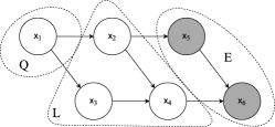
(a) Prior directed graph of generative model $\mathcal{M}$,

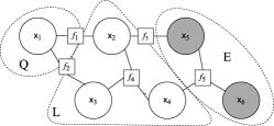
(b) Corresponding rior factor graph $\mathcal{G}$,

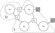
(c) Posterior factor graph $\mathcal{G}^{*}$,

Figure 1: The graphical model structures: (a) prior generative graph, (b) prior factor graph, and (c) posterior factor graph; each with query nodes $\mathscr{Q}=\{1\}$, latent nodes $\mathscr{L}=\{2,3,4\}$, and observed nodes $\mathscr{E}=\{5,6\}$.

In this paper we adopt two perspectives on modelling physical phenomena, constructing an inference method which exploits the strengths of each. Specifically, we harness (1) the Ensemble Kalman filter (EnKF); and (2) Gaussian belief propagation (GaBP), a fusion of generative and probabilistic perspectives.

From the generative perspective, we understand a physical system through its simulated approximation. The Ensemble Kalman Filter (EnKF) [1] is a popular method for state inference using such simulators in e.g. climate-scale modelling. A posterior sample is constructed by ensuring that using it as an input to the simulator produces samples from the observation-conditional distribution. However, the EnKF does not generalise to complicated dependence structures. If we wish to infer latent states jointly with parameters, then we must introduce idiosyncratic approximations [2].

From the probabilistic perspective, models are characterised by joint distributions of random variates. Graphical models [3], typically factorise a joint density over graph $\mathcal{G}$. Message-passing over the edges of $\mathcal{G}$ e.g. using Gaussian Belief propagation (GaBP) [4] infers marginals of interest [5]. This approach is well suited to complex model structures with tractable densities. Message-passing approaches have been effective in various applications, including Bayesian hierarchical models [6, 7], error correcting codes [8, 9], and Simultaneous Locating and Mapping (SLAM) tasks [10, 11]. Their performance may excel where the variables involved are low-dimensional. However, where variables are high-dimensional, the cost of inference may be prohibitive.

Our method, GEnBP borrows strength from both approaches, exploiting the high-dimensional effectiveness of ensemble methods while retaining the ability to handle complex graphical model structures. GEnBP can handle models with noisy and non-linear observation processes, unknown process parameters, and deeply nested hierarchies of dependency between unknown variates, scaling to variables and observations with thousands or millions of dimensions.

II Preliminaries

We introduce the notation, conceptual framework of the model, and the inferential goal.

II-A The generative and probabilistic models

The model state is a random vector $\boldsymbol{\mathsf{x}}$, taking values in $\mathbb{R}^{D}$. We adopt the convention that the state space of a given vector random variate is written in bold, i.e. $\boldsymbol{x}$, and the variate itself in sans-serif, $\boldsymbol{\mathsf{x}}$. For notational clarity, we assume that all variates are continuously distributed with respect to some base measure so that the density $p$ of a variate $\boldsymbol{\mathsf{x}}$ can be written as $\boldsymbol{\mathsf{x}}\sim p(\boldsymbol{x})$; this density is the primary object of interest in the probabilistic perspective.

From a generative perspective we take the state to be generated by simulation. We assume a set of $J$ generating equations $\{\mathcal{P}_{j}\}_{j}$ such that $\mathcal{P}_{j}:\mathbb{R}^{|\mathscr{I}(j)|}\to\mathbb{R}^{|\mathscr{O}(j)|}$, $\boldsymbol{\mathsf{x}}_{\mathscr{I}(j)}\mapsto\boldsymbol{\mathsf{x}}_{\mathscr{O}(j)}$. $\mathscr{I}(j)$ is the set of inputs to the generative equation $\mathcal{P}_{j}$, and $\mathscr{O}(j)$ as the set of outputs. The following conditions must hold for this to define a valid model

1. $\forall j,\mathscr{O}(j)\cap\mathscr{I}(j)=\emptyset$ (no self-loop in a step).

2. If $v\in\mathscr{O}(j)$, then for $k>j$, $v$ appears only in $\mathscr{I}(k)$.

The joint state of the generative model is

$$\begin{bmatrix}\boldsymbol{\mathsf{x}}_{\mathscr{O}(1)}\\ \vdots\\ \boldsymbol{\mathsf{x}}_{\mathscr{O}(J)}\end{bmatrix}=\begin{bmatrix}\mathcal{P}_{1}(\boldsymbol{\mathsf{x}}_{\mathscr{I}(1)})\\ \vdots\\ \mathcal{P}_{J}(\boldsymbol{\mathsf{x}}_{\mathscr{I}(J)})\end{bmatrix}.$$ (1)

The ancestral variables $\mathscr{A}:=\{1,\ldots,D\}\setminus\left(\bigcup_{j}\mathscr{O}(j)\right)$ of the model are those which are not the output of any predictor. By sampling from a the distribution over these ancestral variables then iteratively applying the generative model (1), we obtain samples from the joint prior distribution of all random variates from the model.

The probabilistic interpretation arises from associating densities with the stochastic generating equations, so that $p(\boldsymbol{x}_{\mathscr{O}(j)}|\boldsymbol{x}_{\mathscr{I}(j)})$ quantifies the conditional distribution of the output of the $j$th generating equation given the input. We obtain the prior joint density of all random variates

$$p(\boldsymbol{x})=\prod_{j}p\left(\boldsymbol{x}_{\mathscr{O}(j)}|\boldsymbol{x}_{\mathscr{I}(j)}\right).$$ (2)

This factorisation of the density may be summarised by a graphical model. We refer the reader to the substantial body of literature on that topic [e.g. 3, and references therein].

We divide the variables into three categories: Evidence variables $\mathscr{E}$, which will be observed , latents $\mathscr{L}$, which are unobserved ‘nuisance’ variables, and query variables $\mathscr{Q}$, whose evidence-conditional distribution is our primary interest. In this work, we take the query random variates to be the ancestral variables, denoted as $\mathscr{Q}=\mathscr{A}$. Extending this approach to more general cases is straightforward.

That evidence conditional distribution $\boldsymbol{\mathsf{x}}_{\mathscr{Q}}$ given the evidence variables $\boldsymbol{\mathsf{x}}_{\mathscr{E}}=\boldsymbol{x}_{\mathscr{E}}^{*}$, while marginalising out $\boldsymbol{x}_{\mathscr{L}}$, we refer to as the posterior, we calculate

$$p(\boldsymbol{x}_{\mathscr{Q}}|\boldsymbol{\mathsf{x}}_{\mathscr{E}}{=}\boldsymbol{x}_{\mathscr{E}}^{*}) =\frac{p(\boldsymbol{x}_{\mathscr{Q}},\boldsymbol{x}_{\mathscr{E}}{=}\boldsymbol{x}_{\mathscr{E}}^{*})}{p(\boldsymbol{x}_{\mathscr{E}}{=}\boldsymbol{x}_{\mathscr{E}}^{*})}$$

$$=\frac{\int p(\boldsymbol{x}_{\mathscr{Q}},\boldsymbol{x}_{\mathscr{L}},\boldsymbol{x}_{\mathscr{E}}{=}\boldsymbol{x}_{\mathscr{E}}^{*})\mathrm{d}\boldsymbol{x}_{\mathscr{L}}}{\int p(\boldsymbol{x}_{\mathscr{Q}},\boldsymbol{x}_{\mathscr{L}},\boldsymbol{x}_{\mathscr{E}}{=}\boldsymbol{x}_{\mathscr{E}}^{*})\mathrm{d}\boldsymbol{x}_{\mathscr{Q}}\mathrm{d}\boldsymbol{x}_{\mathscr{L}}}.$$ (3)

II-B Message passing in graphical models

In graphical models we associate a graph structure with the conditional factorisation of the model density (2). An example of the relevant graphs is shown in Fig. 1, starting with the directed graphical model that corresponds to the generative model shown in Fig. 1(a). We refer the reader to the substantial body of literature on that topic [e.g. 3].

In this section, specialise upon belief propagation (BP) [5], applied within the framework of the factor graph [9, 8]. This approximates complex integrals such as (3) using local operations at graph nodes. The factor graph is constructed from the factorisation of the density, where every conditional $p\left(\boldsymbol{x}_{\mathscr{O}(j)}|\boldsymbol{x}_{\mathscr{I}(j)}\right)$ is rewritten as a factor potential $j$, such that $f_{j}(\boldsymbol{x}_{\mathscr{N}(j)})=p\left(\boldsymbol{x}_{\mathscr{O}(j)}|\boldsymbol{x}_{\mathscr{I}(j)}\right)$ where $\mathscr{N}(j):=\mathscr{O}(j)\cup\mathscr{I}(j)$ is the set of neighbours.

$$p(\boldsymbol{x})=\prod_{j}p\left(\boldsymbol{x}_{\mathscr{O}(j)}|\boldsymbol{x}_{\mathscr{I}(j)}\right)=\prod_{j}f_{j}\left(\boldsymbol{x}_{\mathscr{N}(j)}\right).$$ (4)

The associated factor graph $\mathcal{G}$ is bipartite, with a factor node $j$ for each factor potential $f_{j}(\boldsymbol{x}_{\mathscr{N}(j)})$ and a variable node $k$ with each variable $\boldsymbol{\mathsf{x}}_{k}$. Variable nodes are linked by an undirected edge to each factor node in their neighbourhood.

BP estimates a belief over a query node, $b_{\mathcal{G}}(\boldsymbol{x}_{\mathscr{Q}})=\int p(\boldsymbol{x})\mathrm{d}\boldsymbol{x}_{\setminus\mathscr{Q}}$, by integrating out all other variates. As such, it is not the prior graph $\mathcal{G}$ (Fig 1(b)) which produces our quantity of interest (3) but the evidence-conditional graph $\mathcal{G}^{*}$ (Fig 1(c)) obtained by conditioning on $\boldsymbol{\mathsf{x}}_{\mathscr{E}}=\boldsymbol{x}_{\mathscr{E}}^{*}$. We construct $\mathcal{G}^{*}$ from the prior graph $\mathcal{G}$ by altering factors $f_{j},\forall j\in\mathscr{N}(\mathscr{E})$ adjacent to observed variables in the prior factor graph into observation-conditional factors.

$$f_{j}(\boldsymbol{x}_{j})\leftarrow f^{*}_{j}(\boldsymbol{x}_{\mathscr{N}(j)\setminus\mathscr{E}}):=p(\boldsymbol{x}_{\mathscr{N}(j)\setminus\mathscr{E}}|\boldsymbol{\mathsf{x}}_{\mathscr{E}}{=}\boldsymbol{x}_{\mathscr{E}}^{*}).$$ (5)

Our target is now the evidence-conditional belief $p(\boldsymbol{x}_{\mathscr{Q}}|\boldsymbol{\mathsf{x}}_{\mathscr{E}}{=}\boldsymbol{x}_{\mathscr{E}}^{*})=b_{\mathcal{G}^{*}}(\boldsymbol{x}_{\mathscr{A}})$, which we approximate using the following proposition.

Proposition 1 (Belief Propagation on Factor Graphs).

The following messages,

$$m_{f_{j}\rightarrow\boldsymbol{\mathsf{x}}_{k}} =\int\bigg{(}f_{j}\left(\boldsymbol{x}_{\mathscr{N}(j)}\right)\prod_{i\in\mathscr{N}(j)\setminus k}m_{\boldsymbol{\mathsf{x}}_{i}\rightarrow f_{j}}\bigg{)}\mathrm{d}{\boldsymbol{x}_{\mathscr{N}(j)\setminus{k}}}$$ (6)

$$m_{\boldsymbol{\mathsf{x}}_{k}\rightarrow f_{j}} =\prod_{s\in\mathscr{N}(k)\setminus j}m_{f_{s}\rightarrow\boldsymbol{\mathsf{x}}_{k}},$$ (7)

iteratively propagated between all the nodes in the associated factor graph, yield the approximate marginal distribution at target variable node $b(\boldsymbol{x}_{k})=\int p(\boldsymbol{x})\mathrm{d}\boldsymbol{x}_{\setminus k}$,

$$b\left(\boldsymbol{x}_{k}\right) =\prod_{s\in\mathscr{N}(k)}m_{f_{s}\rightarrow\boldsymbol{\mathsf{x}}_{k}}.$$ (8)

The fixed points of this iteration are the fixed points of the Bethé approximation to the target marginal.

Proof.

See Yedidia et al. [12]. ∎

The specific operations to implement BP using these messages are given in Appendix B for the Gaussian case. We follow Ortiz et al. [11], Davison and Ortiz [13] and assume a synchronous message passing schedule, which is well-behaved for a broad class of models. The convergence to a fixed point of a Bethé approximation is a weak guarantee, but widely relied upon in practice. We refer the reader to the extensive literature on convergence results for more detail [14, 4, 15, 16, 17].

Definition 1 (Requisite BP operations).

Partitioning $\boldsymbol{x}_{j}$ so that the density $f\left(\boldsymbol{x}_{j}\right)=f\left(\begin{bmatrix}\boldsymbol{x}_{k}\\ \boldsymbol{x}_{\ell}\end{bmatrix}\right)$, we introduce the operations

Conditioning: $$f\left(\boldsymbol{x}_{j}\right),\boldsymbol{x}_{k}^{*}\mapsto f^{*}(\boldsymbol{x}_{\ell}):=f(\boldsymbol{x}_{\ell}|\boldsymbol{\mathsf{x}}_{k}=\boldsymbol{x}_{k}^{*});$$ (9)

Marginalisation: $$f(\boldsymbol{x}_{j})\mapsto f(\boldsymbol{x}_{k}):=\int f(\boldsymbol{x}_{j})\mathrm{d}\boldsymbol{x}_{\ell};$$ (10)

Multiplication: $$f^{\prime}(\boldsymbol{x}_{j}),f(\boldsymbol{x}_{k})\mapsto f(\boldsymbol{x}_{j}):=f^{\prime}(\boldsymbol{x}_{j})f(\boldsymbol{x}_{k}).$$ (11)

$f$ and $f^{\prime}$ simply denote arbitrary density functions over the argument; and $f^{*}$ denotes a density that is conditional on the elements not present in its argument. The rest of the paper hinges upon the following proposition.

Proposition 2.

To calculate the marginal belief over a target variable $\boldsymbol{\mathsf{x}}_{\mathscr{Q}}$ by message passing in a observation-conditional factor graph (5) starting from (4), a sufficient set of operations defined over factors and variables is (9), (10) and (11).

Proof.

See Appendix I ∎

II-C Gaussian distributions in belief propagation

BP is notably tractable in the case that all factors are Gaussian, [12] (GaBP), which we now introduce. The moments-form Gaussian density m

$$\phi_{M}(\boldsymbol{x};\boldsymbol{m},K)=|2\pi\mathrm{K}|^{-\nicefrac{{1}}{{2}}}\mathrm{e}^{-\nicefrac{{1}}{{2}}(\boldsymbol{x}-\boldsymbol{m})^{\top}\mathrm{K}^{-1}(\boldsymbol{x}-\boldsymbol{m})}$$ (12)

is parameterised by mean $\boldsymbol{m}$ and covariance matrix $\mathrm{K}$. Alternatively, in canonical form, it is represented as

$$\phi_{C}(\boldsymbol{x};\boldsymbol{n},\mathrm{P})=|\nicefrac{{1}}{{2\pi}}\mathrm{P}|^{\nicefrac{{1}}{{2}}}{(2\pi)^{\nicefrac{{n}}{{2}}}}\mathrm{e}^{-\nicefrac{{1}}{{2}}\boldsymbol{x}^{\top}\mathrm{P}\boldsymbol{x}+\boldsymbol{n}^{\top}\boldsymbol{x}}.$$ (13)

with precision matrix $\mathrm{P}=\mathrm{K}^{-1}$ and information vector $\boldsymbol{n}=\mathrm{P}\boldsymbol{m}$, assuming the necessary inverses exist. If the relationships between variables in $\mathcal{G}$ are linear with additive Gaussian noise and the ancestral distributions are Gaussian then the potential over each factor is Gaussian. In this case, all of the requisite operations of Proposition 1 are available in closed form in terms of Gaussian parameters, [18, 11]. These are written out in full in Appendix C. For our current purposes the most challenging operation is multiplication.

Proposition 3.

The multiplication operation (11) specialised to Gaussians is

$$\phi_{C}^{\prime}(\boldsymbol{x};\boldsymbol{n}^{\prime},\mathrm{P}^{\prime})\phi_{C}^{\prime\prime}(\boldsymbol{x}_{k};\boldsymbol{n}^{\prime\prime},\mathrm{P}^{\prime\prime})=\phi_{C}(\boldsymbol{x};\boldsymbol{n}^{\prime}+\boldsymbol{n}^{\prime\prime},\mathrm{P}^{\prime}+\mathrm{P}^{\prime\prime}).$$ (14)

Proof.

Eustice et al. [19] ∎

In practice, GaBP is frequently applied where the factor potentials are not linear, and where the joint distributions are not Gaussian. In this case, we introduce a further approximation, using linearised propagation of errors to find Gaussian approximating densities to the true target density.

GaBP has well-known limitations when nodes are high-dimensions, scaling unfavourably in terms of memory ($\mathcal{O}(D^{2})$) and compute ($\mathcal{O}(D^{3})$) whenever a $D\times D$ covariance matrix inverted.

II-D Ensemble Kalman Filtering

A well-known method which ameliorates large-$D$ difficulties is Ensemble Kalman Filtering (EnKF).Where the GaBP method summarises inference in terms of the parameters of a Gaussian distribution, the EnKF summarises the joint distribution in terms of an ensemble of Monte Carlo samples. The ensemble is a matrix of $N$ samples, $\mathrm{X}:=\begin{bmatrix}\boldsymbol{x}^{(n)}\end{bmatrix}_{1\leq n\leq N}$ drawn i.i.d. from the prior distribution, $\boldsymbol{x}^{(n)}\sim\phi_{M}(\boldsymbol{x};\boldsymbol{\boldsymbol{m}},\mathrm{K})$. Introducing the matrices $\mathrm{A}_{N}:=\begin{bmatrix}\frac{1}{N}&\cdots&\frac{1}{N}\end{bmatrix}^{\top},\mathrm{B}_{N}:=\begin{bmatrix}1&\cdots&1\end{bmatrix}$ and $\mathrm{C}_{N}:=\mathrm{I}_{N}-\mathrm{A}_{N}\mathrm{B}_{N}$, we define

$$\overline{\mathrm{X}} :=\mathrm{X}\mathrm{A}_{N}$$ (Ensemble mean) (15)

$$\breve{\mathrm{X}} :=\mathrm{X}-\mathrm{X}\mathrm{A}_{N}\mathrm{B}_{N}=\mathrm{X}\mathrm{C}_{N}.$$ (Ensemble deviation) (16)

We hereafter suppress $N$, which is uniquely determined by context. Overloading the mean and variance operations to describe empirical moment of ensembles, we write

$$\widehat{\mathbb{E}}\mathrm{X} =\overline{\mathrm{X}}$$ (17)

$$\widehat{\operatorname{Var}}_{\sigma^{2}}\mathrm{X} ={\textstyle\frac{1}{N-1}}\breve{\mathrm{X}}\breve{\mathrm{X}}^{\top}+\mathrm{V}$$ (18)

$$\widehat{\operatorname{Cov}}(\mathrm{X},\mathrm{Y}) ={\textstyle\frac{1}{N-1}}\breve{\mathrm{X}}\breve{\mathrm{Y}}^{\top}$$ (19)

We take the ensemble statistics to define a Gaussian distribution with the same moments, writing $\boldsymbol{x}\sim\phi_{M}(\boldsymbol{x};\overline{\mathrm{X}},\widehat{\operatorname{Var}}_{\sigma^{2}}\mathrm{X})$ given a matrix of samples $\mathrm{X}$. In this generative setting the prior model ensembles are sampled by ancestral sampling with generative equations (1). If the number of samples is much lower than the number of dimensions the implied covariance,has a nearly-low-rank form, which we leverage throughout. Properties of such matrices are explored in Appendix D.

Diagonal inflation nugget terms such as $\sigma^{2}$ arise repeatedly in this work. Setting $\sigma>0$ is useful for numerical stability, to encode model uncertainty, and for ensuring that the covariance matrix is strictly positive definite and thus invertible. These diagonal terms are in practice algorithm hyperparameters which are selected by standard means such as cross validation.

Two of the BP operations of Prop. 1 are known for the EnKF.

Proposition 4.

Partition $\boldsymbol{\mathsf{x}}_{j}=\begin{bmatrix}\boldsymbol{\mathsf{x}}_{k}\\ \boldsymbol{\mathsf{x}}_{\ell}\end{bmatrix}$ so $\mathrm{X}_{j}=\begin{bmatrix}\mathrm{X}_{k}\\ \mathrm{X}_{\ell}\end{bmatrix}$, and

$$\mathrm{X}_{j}\sim\phi_{M}\left(\begin{bmatrix}\boldsymbol{x}_{k}\\ \boldsymbol{x}_{\ell}\end{bmatrix};\begin{bmatrix}\overline{\mathrm{X}}_{k}\\ \overline{\mathrm{X}}_{\ell}\end{bmatrix},\begin{bmatrix}\widehat{\operatorname{Var}}_{\sigma^{2}}\mathrm{X}_{k}&\widehat{\operatorname{Cov}}(\mathrm{X}_{\ell},\mathrm{X}_{k})\\ \widehat{\operatorname{Cov}}(\mathrm{X}_{k},\mathrm{X}_{\ell})&\widehat{\operatorname{Var}}_{\sigma^{2}}(\mathrm{X}_{\ell})\end{bmatrix}\right).$$ (20)

The ensemble form equivalent of factor conditioning (9) is

$$\mathrm{X}_{j},\boldsymbol{x}_{k}^{*}\mapsto\mathrm{X}_{\ell}+\widehat{\operatorname{Cov}}(\mathrm{X}_{\ell},\mathrm{X}_{k})\widehat{\operatorname{Var}}^{-1}_{\sigma^{2}}(\mathrm{X}_{k})(\boldsymbol{x}_{k}^{*}\mathrm{B}-{\mathrm{X}_{k}})$$ (21)

and marginalisation (10) is simply truncation

$$\mathrm{X}_{j}\mapsto\mathrm{X}_{k}$$ (22)

Further, the computational time cost of (21) is $\mathcal{O}(N^{3}D_{\boldsymbol{\mathsf{x}}_{k}})$

Proof.

See appendix G. ∎

The EnKF method is relatively scalable to high dimensions by taking $N\ll D$ which leads to a favourable computation cost, $\mathcal{O}(N^{2}D_{\boldsymbol{\mathsf{x}}_{k}})$ of conditioning compared to GaBP, which is $\mathcal{O}(D^{3}_{\boldsymbol{\mathsf{x}}_{k}})$. However, EnKF is restricted to graphical models with a state-filtering structure since it lacks the multiplication operation (11) needed for factor-graph-style belief propagation over arbitrary graphs.

The EnKF and GaBP methods possess complementary strengths. In the remainder of this paper, we explore how to effectively combine these strengths to achieve optimal results.

III Gaussian Ensemble Belief Propagation

Table I: Relations in Gaussian Ensemble Belief Propagation

Operations	• Sample • Condition	• Propagate
Graph type	Directed	Factor
Decomposition	$\boldsymbol{\mathsf{x}}_{3}=\mathcal{P}(\boldsymbol{\mathsf{x}}_{1},\boldsymbol{\mathsf{x}}_{2})$	$f(x_{1},x_{2},x_{3})$
Node Parameters	Empirical moments	Canonical parameters

We introduce GEnBP, an algorithm that interleaves between EnKF- and GaBP-type operations, which can perform efficient inference in high-dimensional spaces. In the remainder of this section we introduce the nearly-low-rank Gaussian representation, followed by the operations that efficiently approximate the GaBP but also achieve similar efficiency as the EnKF. Our aim is to approximate the GBP with sampling statistics, itself already an algorithm containing multiple layers of approximation to the true target. Nonetheless, the resulting algorithm is empirically effective on problems of interest. Throughout we regard an approximation $\phi_{M}(\hat{\boldsymbol{m}},\hat{\mathrm{K}})$ to a target Gaussian $\phi_{M}(\boldsymbol{m},\mathrm{K})$ to be the best if $\hat{\boldsymbol{m}}=\boldsymbol{m}$ and $\|\hat{\mathrm{K}}-\mathrm{K}\|_{F}$ is minimised. Statistically, this equates to minimising the Maximum Mean Discrepancy between the two distributions with respect to the polynomial kernel of order 2 [20, Example 3].

Specifically, this entails sampling from the generative prior, conversion to canonical statistics, efficient belief propagation, and then recovering samples to match the updated beliefs. A visual summary is shown in Table I, and a detailed is outlined in Algorithm 1.

Algorithm 1 GEnBP

0:  Graph $\mathcal{G}$, set of generative processes $\{\mathcal{P}_{j}\}_{j}$, observations $\boldsymbol{x}_{\mathscr{E}}$, ancestral sample $\mathrm{X}_{\mathscr{A}}$.

0:  Observation-conditional sample $\mathrm{X}^{*}_{\mathscr{Q}}$.

1:  while not converged do

2:     Sample ensemble from the generative processes $\mathcal{P}_{j}$ on $\mathcal{G}$ using (2)

3:     Convert $\mathcal{G}$ into the conditional graph $\mathcal{G}^{*}$ by conditioning observed factors (5) using (21)

4:     Convert variables and factors to nearly-low-rank canonical form {Sec. III-A}

5:     Propagate low-rank messages on $\mathcal{G}^{*}$ {Sec. III-B}

6:     Conform ancestral nodes to belief $\mathrm{X}^{*}_{\mathscr{Q}}\sim b_{\mathcal{G}^{*}}(\mathsf{x}_{\mathscr{A}})$ {Sec. III-D}

7:  end while

8:  Return Approximate marginal sample $\mathrm{X}^{*}_{\mathscr{Q}}$.

III-A Nearly-low-rank Gaussian parameters

The workhorse is the efficient computation by nearly-low-rank Gaussian moments induced by the ensemble samples. This enables translation between ensembles, and their various parameterisation of Gaussians, and efficient operations upon those parameters.

Definition 2.

A positive-definite, symmetric matrix $\mathrm{K}\in\mathbb{R}^{D\times D}$ is nearly-low-rank if $\mathrm{K}=\mathrm{V}\pm\mathrm{L}\mathrm{L}^{\top}$ where $\mathrm{L}\in\mathbb{R}^{D\times N}$ is a low rank component matrix with $N\ll D$ by assumption and $\mathrm{V}=\operatorname{diag}(\boldsymbol{v})$ is a $D\times D$ diagonal matrix

Specifically the empirical variance we use in the EnKF (18) has such a low rank structure with component $\mathrm{L}={\textstyle\frac{1}{\sqrt{N-1}}}\breve{\mathrm{X}}$ and diagonal $\mathrm{V}=\sigma^{2}\mathrm{I}$. Properties of such matrices are expanded in App. D.

Proposition 5.

Suppose $\boldsymbol{\mathsf{x}}\sim\phi_{M}(\cdot;\boldsymbol{m},\mathrm{K})$ has nearly-low-rank variance $\mathrm{K}=\mathrm{L}\mathrm{L}^{\top}+\mathrm{V}$, $\mathrm{L}\in\mathbb{R}^{D\times N}$. Then we may find the parameters of the equivalent canonical form density $\phi_{C}(\cdot;\boldsymbol{n},\mathrm{P})$ as $\boldsymbol{n}=\mathrm{P}\boldsymbol{m}$ and nearly-low-rank precision $\mathrm{P}=\mathrm{K}^{-1}=\mathrm{U}-\mathrm{R}\mathrm{R}^{\top}$, at a time cost of $\mathcal{O}(N^{3}D)$. Further, we may recover the moments-form parameters at the same cost.

Proof.

Appendix D-C ∎

This is the initialises the belief-propagation stage of the algorithm (step 4), setting the distribution for each factor $f_{j}^{*}$ to the empirical distribution of ensemble at that factor, $\mathrm{X}_{j}$,

$$f^{*}_{j}\sim\phi_{M}(\boldsymbol{x};\overline{\mathrm{X}}_{j},\widehat{\operatorname{Var}}_{\gamma^{2}}\mathrm{X}).$$ (23)

III-B Nearly-low-rank belief propagation

The nearly-low-rank representation provides a convenient means of performing the density multiplication operation (14) on the Gaussian statistics.

Proposition 6.

Suppose we are given two canonical-form Gaussian densities with respective information and precisions $\boldsymbol{n}^{\prime},\mathrm{P}^{\prime}$ and $\boldsymbol{n}^{\prime\prime},\mathrm{P}^{\prime\prime}$, where the precisions are both nearly low rank, $\mathrm{P}^{\prime}=\mathrm{U}^{\prime}-\mathrm{R}^{\prime}\mathrm{R}^{\prime\top}$ and $\mathrm{P}^{\prime\prime}=\mathrm{U}^{\prime\prime}-\mathrm{R}^{\prime\prime}\mathrm{R}^{\prime\prime}{}^{\top}$ and $\mathrm{R}^{\prime}\in\mathbb{R}^{D\times N^{\prime}}$ and $\mathrm{R}^{\prime\prime}\in\mathbb{R}^{D\times N^{\prime\prime}}$ and $\mathrm{U}^{\prime},\mathrm{U}^{\prime\prime}$ diagonal. Then the parameters $\boldsymbol{n},\mathrm{P}$ of the multiplied density $\phi_{C}(\cdot,\boldsymbol{n},\mathrm{P})=\phi_{C}(\cdot,\boldsymbol{n}^{\prime},\mathrm{P}^{\prime})\phi_{C}(\cdot,\boldsymbol{n}^{\prime\prime},\mathrm{P}^{\prime\prime})$ are given by

$$\mathrm{P}=\mathrm{P}^{\prime}+\mathrm{P}^{\prime\prime}=\mathrm{U}-\mathrm{R}\mathrm{R}^{\top}$$ (24)

where

$$\mathrm{U} =\mathrm{U}^{\prime}+\mathrm{U}^{\prime\prime},$$ (25)

$$\mathrm{R} =\begin{bmatrix}\mathrm{R}^{\prime}&\mathrm{R}^{\prime\prime}\end{bmatrix}\text{ and }$$ (26)

$$\boldsymbol{n} =\boldsymbol{n}^{\prime}+\boldsymbol{n}^{\prime\prime}.$$ (27)

The new precision matrix is also nearly-low-rank, with component $\mathrm{R}\in\mathbb{R}^{D\times(N^{\prime}+N^{\prime\prime})}$.

Proof.

Follows from (34) and (36) in the appendix. ∎

III-C GEnBP messages

After initialisation, we convert initial factors (23) into canonical form, and proceed to calculate (7), (6) and (8) by applying these operations in various order. The most complicated step is the factor-to-variable message (6), which calculates the moments of the marginal distribution of a variable node $\boldsymbol{\mathsf{x}}_{\ell}$ given a factor node $\boldsymbol{\mathsf{x}}_{k}$, i.e. the factor-to-variable message $f_{j}\to\boldsymbol{\mathsf{x}}_{k}$. This is given by Algorithm 2 for a single incoming message $\boldsymbol{\mathsf{x}}_{\ell}\to f_{j}$. Generalisation to multiple incoming messages is straightforward through iterative application of the algorithm. Variable-to-factor messages are a degenerate case of Algorithm 2, and are omitted.

Algorithm 2 GEnBP $f_{j}\to\boldsymbol{\mathsf{x}}_{k}$ factor-to-variable message with a single incoming message $\boldsymbol{\mathsf{x}}_{\ell}\to f_{j}$.

0:  Gaussian factor canonical parameters for $f_{j}$, $\boldsymbol{n}=\begin{bmatrix}\boldsymbol{n}_{\ell}\\ \boldsymbol{n}_{k}\end{bmatrix},\mathrm{P}=\mathrm{U}-\begin{bmatrix}\mathrm{R}_{\ell}\\ \mathrm{R}_{k}\end{bmatrix}\begin{bmatrix}\mathrm{R}_{\ell}\\ \mathrm{R}_{k}\end{bmatrix}^{\top}$ for $\mathrm{U}=\operatorname{diag}\left(\begin{bmatrix}\boldsymbol{u}_{\ell}\\ \boldsymbol{u}_{k}\end{bmatrix}\right)$ with $\mathrm{R}_{\ell}\in\mathbb{R}^{D_{\ell}\times N},\mathrm{R}_{k}\in\mathbb{R}^{D_{k}\times N}$

0:  $\boldsymbol{\mathsf{x}}_{k}\to f_{j}$ Gaussian message parameters $\boldsymbol{n}^{\prime}_{k}\in\mathbb{R}^{D_{k}}$ and precision $\mathrm{P}_{k}=\mathrm{U}^{\prime}_{k}-\mathrm{R}^{\prime}_{k}\mathrm{R}^{\prime}_{k}{}^{\top}$ with $\mathrm{R}^{\prime}_{k}\in\mathbb{R}^{D_{k}\times N^{\prime}}$ and $\mathrm{U}^{\prime}=\operatorname{diag}\left(\boldsymbol{u}^{\prime}_{k}\right)$

0:  $f_{j}\to\boldsymbol{\mathsf{x}}_{\ell}$ Gaussian message parameters $\boldsymbol{n}^{\prime}_{\ell}$, $\mathrm{P}^{\prime}_{\ell}=\mathrm{U}^{\prime}_{\ell}-\mathrm{R}_{\ell}^{\prime}\mathrm{R}_{\ell}^{\prime}{}^{\top}$

1:  Form joint information vector $\boldsymbol{n}_{\text{prod}}=\begin{bmatrix}\boldsymbol{n}_{\ell}\\ \boldsymbol{n}_{k}+\boldsymbol{n}^{\prime}_{k}\end{bmatrix}$.

2:  Form joint precision $\mathrm{P}_{\text{prod}}=\mathrm{U}_{\text{prod}}-\mathrm{R}_{\text{prod}}\mathrm{R}_{\text{prod}}^{\top}$, $\mathrm{R}_{\text{prod}}=\begin{bmatrix}\mathrm{R}_{\ell}&\mathrm{0}\\ \mathrm{R}_{k}&\mathrm{R}^{\prime}_{k}\end{bmatrix}$ and $\mathrm{U}_{\text{prod}}=\operatorname{diag}\left(\begin{bmatrix}\boldsymbol{u}_{\ell}\\ \boldsymbol{u}_{k}+\boldsymbol{u}^{\prime}_{k}\end{bmatrix}\right)$

3:  Form joint covariance $\mathrm{K}_{\text{prod}}=\mathrm{P}_{\text{prod}}^{-1}=\mathrm{V}_{\text{prod}}+\mathrm{L}_{\text{prod}}\mathrm{L}_{\text{prod}}^{\top}$ where $\mathrm{L}_{\text{prod}}\in\mathbb{R}^{(D_{k}+D_{k})\times(N+N^{\prime})}$ and $\mathrm{V}=\operatorname{diag}(\boldsymbol{v}_{\text{prod}})$

4:  Calculate joint mean $\boldsymbol{m}_{\text{prod}}=\mathrm{P}_{\text{prod}}\boldsymbol{n}_{\text{prod}}$

5:  Form the marginal mean over $\boldsymbol{\mathsf{x}}_{\ell}$, $\boldsymbol{m}_{\ell}=\boldsymbol{m}_{\text{prod}}[1:D_{k}]$

6:  Form the marginal covariance over $\boldsymbol{\mathsf{x}}_{\ell}$, $\mathrm{K}_{\ell}=\mathrm{V}_{\ell}+\mathrm{L}_{\ell}\mathrm{L}_{\ell}^{\top}$ where $\mathrm{L}_{\text{prod}}[1:D_{k},1:(N^{\prime}+N)]$, $\mathrm{V}_{\ell}=\operatorname{diag}(\boldsymbol{v}_{\text{prod}}[1:D_{k}])$

7:  Constrain the rank of $\mathrm{K}_{\ell}\leftarrow\mathrm{K}_{\ell}^{\prime}=\mathrm{V}_{\ell}+\mathrm{L}_{\ell}^{\prime}\mathrm{L}_{\ell}^{\prime}{}^{\top}$ to $N$ setting $\mathrm{L}_{\ell}^{\prime}=\mathrm{A}\mathrm{S}$ for $\mathrm{A}$ the left singular vectors and $\mathrm{S}$ the top $n$ singular values

8:  Calculate the marginal precision $\mathrm{P}^{\prime}_{\ell}=\mathrm{K}_{\ell}^{-1}=\mathrm{U}_{\ell}-\mathrm{R}_{\ell}\mathrm{R}_{\ell}^{\top}$

9:  Calculate the marginal information vector $\boldsymbol{n}^{\prime}_{\ell}=\mathrm{P}^{\prime}_{\ell}\boldsymbol{m}_{\ell}$

10:  Return canonical information vector $\boldsymbol{n}^{\prime}_{\ell}$

11:  Return canonical precision $\mathrm{P}^{\prime}_{\ell}$

This step is one of the most costly. Suppose factor node $f$ has dimension $D$, and $K$ neighbours, and we wish to calculate an outgoing message to a variable node of dimension $d$. In the worst case, there are messages from all $K-1$ neighbours, so the concatenated components of the factor belief precision matrix in step 2 is a $D\times NK$ matrix. Inverting this in step 3 has a cost of $\mathcal{O}(DN^{3}K^{3})$ (Prop 9). We approximate this covariance matrix in the Frobenius norm using SVD, using D-E at a cost of $\mathcal{O}(DNK\log N+N^{2}(D+NK))$ using the method of [21, 6.1]. Marginalising by truncating the moments to the $d$ dimensions spanned by the variable node leaves us with $d\times N$ variance component matrices. The canonical form of the reduced-rank belief may be found with time cost of $\mathcal{O}(N^{3}d)$ using 10. Collecting dominant terms, the overall cost of factor-to-node messages is $\mathcal{O}(DN^{3}K^{3}).$

III-D Nearly-low-rank ensemble recovery

Recovering an ensemble whose parameters are consistent with the posterior belief $b(\boldsymbol{\mathsf{x}}_{\mathscr{Q}})=\phi_{M}(\boldsymbol{x}_{\mathscr{Q}};\boldsymbol{m}_{\mathscr{Q}},\mathrm{K}_{\mathscr{Q}})$ at a given query node $\mathscr{Q}$ returns us an ensemble representation. Suppressing the $\mathscr{Q}$ subscript, we seek a transformation $T$ which maps the prior ensemble $\mathrm{X}\in\mathbb{R}^{D\times M}$ to an ensemble $T(\mathrm{X})$ with moments as close as possible to $\mathrm{K}=\mathrm{V}-\mathrm{L}\mathrm{L}^{\top}$, $\mathrm{V}=\operatorname{diag}(\boldsymbol{v})$ and $\mathrm{L}\in\mathbb{R}^{D\times N}$. We restrict ourselves to affine transformations

$$T:\mathrm{X}\mapsto\boldsymbol{\mu}\mathrm{B}+\breve{\mathrm{X}}\mathrm{T},$$ (28)

leaving the parameters $\boldsymbol{\mu}\in\mathbb{R}^{D},\mathrm{T}\in\mathbb{R}^{M\times M}$ to be chosen. Fixing $\boldsymbol{\mu}\equiv\boldsymbol{m}$, we choose a $\mathrm{T}$ to minimise the Frobenius distance between the covariance matrix of the mapped ensemble and the nearly-low-rank target variance $\mathrm{K}=\mathrm{L}\mathrm{L}^{\top}+\mathrm{V}$,

$$L(\mathrm{T}) :=\Big{\|}\widehat{\operatorname{Var}}_{\eta^{2}}(\boldsymbol{\mu}\mathrm{B}+\breve{\mathrm{X}}\mathrm{T})-\mathrm{K}\Big{\|}_{F}^{2}$$ (29)

This can be achieved without forming the large $\mathrm{K}\in\mathbb{R}^{D\times D}$. $\mathrm{T}$ is identifiable only up to a unitary transform. We therefore find $\mathrm{M}:=\mathrm{T}\mathrm{T}^{\top}$ from the space of positive definite matrices, and selecting a $\mathrm{T}$ from $\mathrm{M}$ by factorisation.

Proposition 7.

A symmetric positive semi-definite matrix $\mathrm{M}=\mathrm{T}\mathrm{T}^{\top}$ which satisfies

$$\breve{\mathrm{X}}^{\top}\breve{\mathrm{X}}\mathrm{M}\breve{\mathrm{X}}^{\top}\breve{\mathrm{X}} =(N{-}1)\left(\breve{\mathrm{X}}^{\top}\mathrm{L}(\breve{\mathrm{X}}^{\top}\mathrm{L})^{\top}-\breve{\mathrm{X}}^{\top}(\mathrm{V}-\boldsymbol{\eta}\mathrm{I})\breve{\mathrm{X}}\right).$$

defines a transform (28) which minimises (29). Further, for $\mathrm{M}$ may be found with a memory complexity $\mathcal{O}(M^{2}+N^{2})$ and a time complexity $\mathcal{O}(N^{3}+DN^{2}+DM^{2})$.

Proof.

Appendix H∎

For a variable with $K$ neighbours, the worse-case is $M=KN$ so the cost comes to $\mathcal{O}(N^{3}+DN^{2}K^{2})$. The cost of finding the target covariance from the belief precision is $\mathcal{O}(DM^{3})=(DK^{3}N^{3})$ using (42) which dominates, so our total cost for ensemble recovery is $\mathcal{O}(DK^{3}N^{3})$.

III-E Total computational cost

Analysis of the computational cost of the GEnBP algorithm depends upon graph structure and the various tuning parameters. The size of the ensemble in GEnBP is a free parameter controlling the fidelity of the approximation to classical GaBP, and also the computational cost. Empirically, in many useful problems $N\ll D$ (App. A-B). Detailed costs are collated in Tab II in App. J; Notably GEnBP is favourable for all operations for bounded factor degree $K$.

Some care is needed in the interpretation of costs involving the node degree $K$. For $D$ large GEnBP dominates GaBP algorithm, which attains a cost of $\mathcal{O}(D^{3})$ unless $K$ is also large. In the system identification case $K$ may be very large, since the latent parameter influence every timestep so has many neighbours. We can reduce the size of large factor nodes, at the cost of introducing additional nodes by decomposing those factors into a chain of smaller factor and variable nodes nodes with equality constraints, the Forney factorisation. This modification does not alter the models’ marginal distributions [22], but controls $K$. In our later system identification example, this caps $K\leq 4$, but at the cost of requiring more messages to be passed. The net impact depends upon the graphical structure of the specific problem, but in our examples, the cost of the additional messages is outweighed by the reduction in the cost of the factor-to-variable messages.

IV Experiments

GEnBP was compared against GaBP in two synthetic benchmark challenges. The first is a 1d transport problem while the second is a more complex 2d fluid dynamics problem. We fix the model structure, evidence and query in both to define a system identification problem (Appendix K-A), where a parameter of interest influences a nonlinear dynamical system whose states are noisily observed. We define the problem as

$$\boldsymbol{\mathsf{q}} =\mathcal{P}_{\boldsymbol{\mathsf{q}}}$$

$$\boldsymbol{\mathsf{x}}_{t} =\mathcal{P}_{\boldsymbol{\mathsf{x}}}(\boldsymbol{\mathsf{x}}_{t{\operatorname{-}}1},\boldsymbol{\mathsf{q}}),\quad t=1,2,\cdots,T$$

$$\boldsymbol{\mathsf{y}}_{t} =\mathcal{P}_{\boldsymbol{\mathsf{y}}}(\boldsymbol{\mathsf{x}}_{t}),\quad t=1,2,\cdots,T$$ (30)

where our evidence is $\mathscr{E}=\{\boldsymbol{\mathsf{y}}_{t}=\boldsymbol{y}_{t}\}_{1\leq t\leq T}$ and the query is $\mathscr{Q}=\boldsymbol{\mathsf{q}}$. If $\boldsymbol{\mathsf{q}}$ were known, estimating $\{\boldsymbol{\mathsf{x}}_{t}\}_{t}$ from $\{\boldsymbol{\mathsf{y}}_{t}\}_{t}$ would be a standard filtering problem, soluble by EnKF.

The GaBP experiments use the implementation of Ortiz et al. [11]. That version admits only diagonal prior , whereas GEnBP cannot have a diagonal prior by construction. Other hyperparameters are also not directly comparable. We attempt to ameliorate this mismatch by choosing favourable values for each algorithm by random hyperparameter search on a validation set, selecting the hyperparameters which yield the best posterior likelihood for the group truth $\mathscr{Q}$, specifically the nugget terms $\gamma^{2}$ (23), $\eta^{2}$ (29) and $\sigma^{2}$ (21) and equivalent nugget terms in GaBP.

IV-A 1d transport model

In the transport problem 1-dimensional dynamical system states are subject to transport and diffusion with (Appendix K-B), where the transport term introduces nonlinearity. Observations are partial observations of state perturbed by centred additive Gaussian noise. The simplicity of this model means it is easy to plot and interpret.

Figure 2 shows samples from the prior and posterior distributions inferred for each model. In this synthetic problem we know the ground truth value $q_{0}$ and we evaluate performance by mean squared error (MSE) of the posterior mean estimate $\mathbb{E}b_{\mathcal{G}*}(\boldsymbol{\mathsf{q}})-q_{0}$ and the log-likelihood, $\log b_{\mathcal{G}*}(q_{0};\boldsymbol{\mathsf{q}})$. Both models provide reasonable estimates in terms of MSE in this case, but the GEnBP estimate is able to exploit the nearly-low rank structure of the problem to provide a more accurate estimate with a higher likelihood.

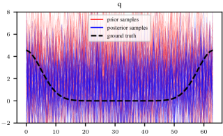
(a) GaBP, $\widehat{\operatorname{MSE}}=1.93,\widehat{\log p}(q|\mathscr{E})=-228$

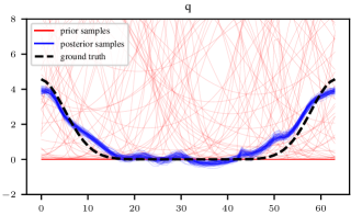
(b) GEnBP, $\widehat{\operatorname{MSE}}=0.167,\widehat{\log p}(q|\mathscr{E})=-49.6$

Figure 2: $N=64$ samples from the posterior mean estimate for the latent $\boldsymbol{\mathsf{q}}$ for the system identification problem with 1d transport dynamics (App K-B).

IV-B 2d fluid dynamics model

In the computational fluid dynamics (CFD) problem, (Appendix K-C) the system states are governed by a high dimensional computational fluid dynamics simulator. This class of problems is of immense practical importance, but typically of high ambient dimension. The parameter of interest is a static latent force $\boldsymbol{\mathsf{q}}$ applied to a fluid in a 2d domain subject to discretised Navier-Stokes equations. The $d\times d$ discretised state is stacked into a vector $\boldsymbol{\mathsf{x}}\in\mathbb{R}^{d^{2}}$. In our 2d incompressible equations the state field and forcing fields are scalar, so $D_{\mathscr{Q}}=D_{\boldsymbol{\mathsf{x}}_{t}}=d^{2}$.

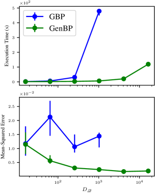
Figure 3: GEnBP performance with increasing problem dimension $D_{\mathscr{Q}}$. Error bars show empirical $50\%$ intervals calculated from $n=10$ independent runs.

Fig 3 demonstrates that GEnBP is able to solve the target with a comparable accuracy and posterior likelihood but at a far higher scale than GaBP. Over large scale problems GEnBP is dominant, achieving comparable MSE, and superior compute time. Note the GBP experiments are truncated because experiments with dimension $D_{\mathscr{Q}}>1024$ failed to complete due to resource exhaustion. In high dimension, GaBP projected completion times were days for problems that GEnBP solved in minutes.

V Conclusions

We have introduced Gaussian Ensemble Belief Propagation (GEnBP), a novel method for solving high-dimensional inference problems in dynamic systems using factor graphs. GEnBP exploits the strengths of two well known methods, the Ensemble Kalman filter and Gaussian belief propagation.

Our findings demonstrate that GEnBP offers two significant advantages. The first is the ability to scale to higher dimensions. Traditional GBP cannot scale. By employing ensemble approximations, GEnBP can accommodate larger and more complex factor graphs making it far more superior to tackle a broad range of real-world problems. The second advantage is the method’s flexibility in model representation. GEnBP can provide a much more flexible representation using factor graph models when compared to EnKF. This flexibility is particularly beneficial in modeling complex systems with intricate dependencies and interactions.

While providing efficiencies through substantial speed up and flexibility, there are some limitations and challenges. First, the ability to scale comes at the cost of introducing additional tuning parameters, which require careful adjustment - a non-trivial task. Second, GEnBP requires an increased number of model executions in the sampling stage, which may be prohibitive for models with long run-times. Finally, similar to GBP, GEnBP is constrained to unimodal posterior distributions. This limitation can be significant in systems where the underlying probability distributions are multimodal, as GEnBP may not capture the full complexity of the distribution.

GEnBP represents a significant advancement in the field of probabilistic graphical models and opens the door to high-dimensional inference problems. Despite its limitations, its scalability and computational efficiency make it a promising approach for a broad range of applications. Future research will focus on continuing to refine and extend GEnBP for complex systems modelling. Specifically our focus will be on developing strategies for automatically tuning the many parameters defined in the GEnBP. Incorporating the many tricks and optimisations from the GaBP literature, such as graph pruning for improved computational efficiency [19] or handling outliers using robust distributions [23] would further extend the impact of these results.

ar

Appendix A Experimental details and additional results

A-A Hardware configuration

Timings are on conducted on Dell PowerEdge C6525 Server AMD EPYC 7543 32-Core Processors running at 2.8 GHz ( 3.7 GHz turbo) with 256 MB cache. Float sizes are set to 64 bits for all calculations. Memory limit is capped to 32Gb. Execution time is capped to 119 minutes.

A-B Ensemble size

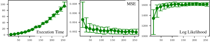
Figure 4: Performance of GEnBP with varying ensemble size $N$ for the 1d transport system identification problem (App K-B). Confidence intervals are empirical $95\%$ intervals based on $n=80$ independent runs.

Appendix B Factor Graph Belief Propagation

Following the terminology of Ortiz et al. [11], we describe the factor graph belief propagation algorithm for generic factor graphs.

Algorithm 3 Loopy Low-rank Belief Propagation over Factor Graph $\mathcal{G}$

0:  Factor graph $\mathcal{G}$ with variable nodes $\{\boldsymbol{\mathsf{x}}_{k}\}_{k}$ and factor nodes $\{f_{j}\}_{j}$

0:  Initial messages ${\boldsymbol{\mathsf{x}}_{k}\to f_{j}}$ and ${f_{j}\to\boldsymbol{\mathsf{x}}_{k}}$

0:  Approximate marginal beliefs $b(\boldsymbol{\mathsf{x}}_{k})$ for all $\boldsymbol{\mathsf{x}}_{k}\in\mathcal{G}$

1:  Initialize message queues $Q_{\boldsymbol{\mathsf{x}}_{k}\to f_{j}}$ and $Q_{f_{j}\to\boldsymbol{\mathsf{x}}_{k}}$ to be empty

2:  while not converged do

3:     for each factor $f_{j}\in\mathcal{G}$ do

4:        for each variable $\boldsymbol{\mathsf{x}}_{k}\in\mathscr{N}(f_{j})$ do

5:           Send factor to variable message (6) to each neighbour

6:        end for

7:     end for

8:     for each variable $\boldsymbol{\mathsf{x}}_{k}\in\mathcal{G}$ do

9:        for each factor $f_{j}\in\mathscr{N}(\boldsymbol{\mathsf{x}}_{k})$ do

10:           Send variable to factor message (7) to each neighbour

11:        end for

12:        Update belief $b(\boldsymbol{x}_{k})$ (8)

13:     end for

14:     Check for convergence criteria

15:  end while

16:  Return $b(\boldsymbol{\mathsf{x}}_{k})$ for all $\boldsymbol{\mathsf{x}}_{k}\in\mathcal{G}$

Appendix C Gaussian Factor updates

We write $\phi_{M}\left(\boldsymbol{x};\boldsymbol{m},\mathrm{K}\right)$ for $\phi_{M}$ the Gaussian density with parameters mean $\boldsymbol{m}$ and covariance $\mathrm{K}$.

Proposition 8.

As in Proposition 1, we partition the random vector $\boldsymbol{\mathsf{x}}_{j}\sim\phi_{M}\left(\begin{bmatrix}\boldsymbol{x}_{k}\\ \boldsymbol{x}_{\ell}\end{bmatrix};\begin{bmatrix}\boldsymbol{m}_{k}\\ \boldsymbol{m}_{\ell}\end{bmatrix},\begin{bmatrix}\mathrm{K}_{{k}{k}}&\mathrm{K}_{{k}{\ell}}\\ \mathrm{K}_{{\ell}{k}}&\mathrm{K}_{{\ell}{\ell}}\end{bmatrix}\right)$. We define $\hat{\mathrm{K}}:=(\mathrm{K}_{{j}{j}}^{-1}+\mathrm{K}^{\prime}_{{j}{j}}{}^{-1})^{-1}$. Where the node and factors are Gaussian, the operations of Proposition 1 have the following form,

Conditioning: $$\phi_{M}\left(\boldsymbol{x}_{j};\boldsymbol{m}_{j},\mathrm{K}_{jj}\right),\boldsymbol{x}_{{k}}^{*}\mapsto\phi_{M}(\boldsymbol{x}_{\ell};\boldsymbol{m}_{\ell}+\mathrm{K}_{{\ell}{k}}\mathrm{K}_{{k}{k}}^{-1}(\boldsymbol{x}_{{k}}^{*}-\boldsymbol{m}_{k}),\mathrm{K}_{{\ell}{\ell}}-\mathrm{K}_{{\ell}{k}}\mathrm{K}_{{k}{k}}^{-1}\mathrm{K}_{{k}{\ell}});$$ (31)

Marginalisation: $$\phi_{M}\left(\boldsymbol{x}_{j};\boldsymbol{m}_{j},\mathrm{K}_{{j}{j}}\right)\mapsto\phi_{M}\left(\boldsymbol{x}_{k};\boldsymbol{m}_{k},\mathrm{K}_{{k}{k}}\right);$$ (32)

Multiplication: $$\phi_{M}^{\prime}\left(\boldsymbol{x}_{j};\boldsymbol{m}^{\prime}_{j},\mathrm{K}^{\prime}_{{j}{j}}\right),\phi_{M}\left(\boldsymbol{x}_{k};\boldsymbol{m}_{k},\mathrm{K}_{{k}{k}}\right)\mapsto\phi_{M}\left(\boldsymbol{x}_{j};\hat{\mathrm{K}}(\mathrm{K}_{{j}{j}}^{-1}\boldsymbol{m}_{j}+\mathrm{K}^{\prime}_{{k}{k}}{}^{-1}\boldsymbol{m}^{\prime}_{j}),\hat{\mathrm{K}}\right);$$ (33)

$$\phi_{C}^{\prime}\left(\boldsymbol{x}_{j};\boldsymbol{n}^{\prime}_{j},\mathrm{P}^{\prime}_{{j}{j}}\right),\phi_{C}\left(\boldsymbol{x}_{k};\boldsymbol{n}_{k},\mathrm{P}_{{k}{k}}\right)\mapsto\phi_{C}\left(\boldsymbol{x}_{j};\boldsymbol{n}^{\prime}_{j}+\boldsymbol{n}_{j},\mathrm{P}^{\prime}+\mathrm{P}\right).$$ (34)

Proof.

e.g. Bickson [18]. ∎

Appendix D Nearly-low-rank matrices

Suppose the $\mathrm{K}=\mathrm{V}+k\mathrm{L}{\mathrm{L}}^{\top}$ where $\mathrm{L}$ is a $D\times N$ matrix, $\mathrm{I}$ is $D\times D$ and $\mathrm{V}=\operatorname{diag}(\boldsymbol{v}$ and $k\in\{-1,1\})$ is the sign of the matrix. We are primarily interested in such matrices in the case that $N\ll D$, which case we have called nearly-low-rank, when their computational properties are favourable for our purposes. This is in contrast to matrices with no particular exploitable structure, which we refer to as dense.

Throughout this section we assume that the matrices in question are positive definite; and that all operations are between conformable operations. We refer to the matrix $\mathrm{L}$ as the component of the nearly-low-rank matrix, and the diagonal matrix $\mathrm{V}$.

If $N\geq D$ the name is misleading since they are not truly low-rank; the identities we write here still hold, but are not computationally expedient.

D-A Multiplication by a dense matrix

The matrix product of an arbitrary matrix with a nearly-low-rank matrix may be calculated efficiently by grouping operations, since $\mathrm{K}\mathrm{X}=\mathrm{V}\mathrm{X}\pm\mathrm{U}(\mathrm{U}^{\top}\mathrm{X})$, which has a time cost of $\mathcal{O}(ND^{2})$ and which may be calculated without forming the full matrix $\mathrm{K}$. The result is not in general also a nearly-low-rank matrix.

D-B Addition

The matrix sum of two nearly-low-rank matrices with the same sign is also a nearly-low-rank matrix. Suppose $\mathrm{K}=\mathrm{V}+k\mathrm{L}\mathrm{L}^{\top},\mathrm{K}^{\prime}=\mathrm{V}^{\prime}+k\mathrm{L}^{\prime}\mathrm{L}^{\prime\top},$

$$\mathrm{K}+\mathrm{K}^{\prime} =\mathrm{V}+\mathrm{V}^{\prime}+k\mathrm{L}\mathrm{L}^{\top}+k\mathrm{L}^{\prime}\mathrm{L}^{\prime\top}$$ (35)

$$=\mathrm{V}+\mathrm{V}^{\prime}+k\begin{bmatrix}\mathrm{L}&\mathrm{L}^{\prime}\end{bmatrix}\begin{bmatrix}\mathrm{L}&\mathrm{L}^{\prime}\end{bmatrix}^{\top}.$$ (36)

The new matrix, is also nearly low rank with has nugget term $\mathrm{V}+\mathrm{V}$ and component $\begin{bmatrix}\mathrm{L}&\mathrm{L}^{\prime}\end{bmatrix}$.

D-C Cheap nearly-low-rank inverses

Inverses of nearly-low-rank matrices are once again nearly-low-rank matrices, and may be found efficiently.

Proposition 9.

Choose nearly-low rank $\mathrm{K}=\mathrm{V}+\mathrm{L}{\mathrm{L}}^{\top}$, i.e. with sign $k$ positive. Then its inverse

$$\mathrm{K}^{-1}=\mathrm{V}^{-1}-\mathrm{R}\mathrm{R}^{\top}$$ (37)

is also nearly-low-rank, of the same component dimension, but with a negative sign, with

$$\mathrm{R}=\mathrm{V}^{-1}{\mathrm{L}}\operatorname{chol}\left(\left(\mathrm{I}+{\mathrm{L}}^{\top}\mathrm{V}^{-1}{\mathrm{L}}\right)^{-1}\right).$$ (38)

where $\operatorname{chol}(\mathrm{A})$ denotes a decomposition $\operatorname{chol}(\mathrm{A})\operatorname{chol}(\mathrm{A})^{\top}=\mathrm{A}$.

Proof.

Using the Woodbury identity,

$$\mathrm{K}^{-1} =\mathrm{V}^{-1}-\mathrm{V}^{-1}{\mathrm{L}}\left(\mathrm{I}+{\mathrm{L}}^{\top}\mathrm{V}^{-1}{\mathrm{L}}\right)^{-1}{\mathrm{L}}^{\top}\mathrm{V}^{-1}$$

$$=\mathrm{V}^{-1}-\mathrm{R}\mathrm{R}^{\top}.$$

∎

Proposition 10.

Choose nearly-low rank $\mathrm{P}=\mathrm{U}-\mathrm{R}\mathrm{R}^{\top}$, i.e. with sign $k$ negative. Then its inverse

$$\mathrm{P}^{-1}=\mathrm{U}^{-1}-\mathrm{L}\mathrm{L}^{\top}$$ (39)

is also nearly-low-rank, of the same component dimension, but with a positive sign, with

$$\mathrm{L}=\mathrm{U}^{-1}{\mathrm{R}}\operatorname{chol}\left(\left(-\mathrm{I}+{\mathrm{R}}^{\top}\mathrm{U}^{-1}{\mathrm{R}}\right)^{-1}\right).$$ (40)

Proof.

Using the Woodbury identity,

$$\mathrm{P}^{-1} =\mathrm{U}^{-1}-\mathrm{U}^{-1}{\mathrm{R}}\left(-\mathrm{I}+{\mathrm{R}}^{\top}\mathrm{U}^{-1}{\mathrm{R}}\right)^{-1}{\mathrm{R}}^{\top}\mathrm{U}^{-1}$$ (41)

$$=\mathrm{U}^{-1}+\mathrm{L}\mathrm{L}^{\top}$$ (42)

∎

If we interpret the $\operatorname{chol}(\mathrm{A})$ operation as the construction of Cholesky factors, the cost of the inversion in either case is the same, $\mathcal{O}\left(N^{2}D+N^{3}\right)$ — $\mathcal{O}(N^{3})$ for the construction of the Cholesky factor, and $\mathcal{O}(DN^{2})$ for the requisite matrix multiplies. The space cost is $\mathcal{O}\left(ND\right)$.

For a given $\mathrm{K}=\mathrm{V}+k\mathrm{L}\mathrm{L}^{\top}$, the term $\left(k\mathrm{I}+{\mathrm{L}}^{\top}\mathrm{V}^{-1}{\mathrm{L}}\right)$ is referred to as the capacitance of the matrix by convention.

D-D Exact inversion when the component is high-rank

Suppose $\mathrm{P}=\mathrm{U}-\mathrm{R}\mathrm{R}^{\top}$ where the $D\times N$ components high rank, in the sense that $N>D$. Then the low rank inversion to calculate $\mathrm{P}^{-1}$ is no longer cheap, since the $\mathcal{O}(N^{D})$ cost is greater than naive inversion of the dense matrix, at $\mathcal{O}(D^{3})$. In this case, it is cheaper to recover a nearly-low-rank inverse by an alternate method. Note that $(\mathrm{U}-\mathrm{P})^{-1}=\mathrm{U}^{-1}-\mathrm{U}^{-1}(\mathrm{U}^{-1}-\mathrm{P}^{-1})^{-1}\mathrm{U}^{-1}$. We find the eigendecomposition

$$\mathrm{P}^{-1} =\mathrm{U}^{-1}+\mathrm{L}\mathrm{L}^{\top}$$ (43)

for some $\mathrm{L}$. Such an $\mathrm{L}$ is given by $\mathrm{L}=\mathrm{Q}\mathrm{\Lambda}^{\nicefrac{{1}}{{2}}}$ for $\mathrm{Q}\mathrm{\Lambda}\mathrm{Q}^{\top}=\mathrm{P}^{-1}-\mathrm{U}^{-1}$ a spectral decomposition. In the case that the diagonal $\mathrm{U}$ is constant this may be found more efficiently.

If, instead, we wish to invert $\mathrm{K}=\mathrm{V}+\mathrm{L}\mathrm{L}^{\top}$ we need to find $(-\mathrm{V}+\mathrm{K})^{-1}=-\mathrm{V}^{-1}-\mathrm{V}^{-1}(\mathrm{K}^{-1}-\mathrm{V}^{-1})^{-1}\mathrm{V}^{-1}$, so we decompose instead $\mathrm{Q}\mathrm{\Lambda}\mathrm{Q}=\mathrm{V}^{-1}(\mathrm{K}^{-1}-\mathrm{V}^{-1})^{-1}\mathrm{V}^{-1}$ and define $\mathrm{R}=\mathrm{Q}\mathrm{\Lambda}^{-\nicefrac{{1}}{{2}}}$. Then the nearly-low-rank form of the inverse is $-\mathrm{V}^{-1}-\mathrm{R}\mathrm{R}^{\top}$.

D-E Reducing component rank

We use the SVD to efficiently reduce the rank of the components in the nearly-low-rank matrix in the sense of finding a Frobenius-distance-minimising approximation.

Suppose $\mathrm{K}=\mathrm{V}+\mathrm{L}{\mathrm{L}}^{\top}$ where $\mathrm{L}$ is a $D\times N$ matrix, $\mathrm{I}$ is $D\times D$ and $\mathrm{V}=\operatorname{diag}(\boldsymbol{v})$. Let $\mathrm{Y}\mathrm{S}\mathrm{Z}^{\top}$ be the “thin” SVD of $\mathrm{L}$, i.e. $\mathrm{Y}\in\mathbb{R}^{D\times N},\mathrm{S}\in\mathbb{R}^{N\times N},\mathrm{Z}\in\mathbb{R}^{N\times N}$ with $\mathrm{Y}^{\top}\mathrm{Y}=\mathrm{I}_{N},\mathrm{Z}^{\top}\mathrm{Z}=\mathrm{I}_{N}$, and $\mathrm{S}$ diagonal with non-negative entries. Then

$$\mathrm{L}\mathrm{L}^{\top} =\mathrm{Y}\mathrm{S}\mathrm{Z}^{\top}\mathrm{Z}\mathrm{S}\mathrm{Y}^{\top}=\mathrm{Y}\mathrm{S}^{2}\mathrm{Y}^{\top}.$$

First we note that should any singular values in $\mathrm{S}$ be zero, we may remove the corresponding columns of $\mathrm{Y}$ and $\mathrm{Z}$ without changing the product, so their exclusion is exact. Next, we note that if we choose the largest $M$ singular values of $\mathrm{S}$, setting the rest to zero, we obtain a Frobenius approximation of $\mathrm{L}\mathrm{L}^{\top}$ of rank $M$.

An SVD that captures the top $M$ singular values has naive computational cost of $\mathcal{O}(DN^{2})$ or may be found by randomised methods at a cost of $\mathcal{O}(ND\log M+M^{2}(D+N))$ [21, 6.1].

Appendix E Gaussians with nearly-low-rank parameters

We recall the forms of the Gaussian density introduced in section II-C, T moments form using the mean $\boldsymbol{m}$ and covariance matrix $\mathrm{K}$,

$$\boldsymbol{\mathsf{x}} \sim\mathcal{N}(\boldsymbol{m},\mathrm{K})=\mathcal{N}(\mathbb{E}[\boldsymbol{\mathsf{x}}],\operatorname{Var}(\boldsymbol{\mathsf{x}})).$$

and the canonical form,

$$\boldsymbol{\mathsf{x}} \sim\mathcal{N}_{C}(\boldsymbol{n},\mathrm{P})=\mathcal{N}_{C}(\operatorname{Var}^{-1}(\boldsymbol{\mathsf{x}})\mathbb{E}[\boldsymbol{\mathsf{x}}],\operatorname{Var}^{-1}(\boldsymbol{\mathsf{x}})).$$

which uses the information vector $\boldsymbol{n}$ and the precision matrix, $\mathrm{P}$ with $\boldsymbol{n}=\mathrm{K}^{-1}\boldsymbol{m},\quad\mathrm{P}=\mathrm{K}^{-1}$. The (equivalent) densities induced by these parameterisations are

$$f(\boldsymbol{x})\propto\frac{1}{2}(\boldsymbol{x}-\boldsymbol{m})^{\top}\mathrm{K}^{-1}(\boldsymbol{x}-\boldsymbol{m})=\frac{1}{2}\boldsymbol{x}^{\top}\mathrm{P}\boldsymbol{x}-\boldsymbol{n}^{\top}\boldsymbol{x}$$

We associate a given Gaussian ensemble with a moments-form Gaussian in the natural way,

$$\mathrm{X}_{\sigma^{2}} \sim\mathcal{N}(\boldsymbol{m},\mathrm{K})=\mathcal{N}(\widehat{\mathbb{E}}[\mathrm{X}],\widehat{\operatorname{Var}}_{\sigma^{2}}(\mathrm{X}))$$

introducing a parameter $\sigma^{2}$ which we use to ensure invertibility of the covariance if needed.

We associate with each moments-form Gaussian a canonical form which may be cheaply calculated by using the by using the low-rank representation of the covariance prop 9,

$$\mathrm{X}_{\sigma^{2}} \sim\mathcal{N}(\boldsymbol{m},\mathrm{K})$$

$$\boldsymbol{m} =\widehat{\mathbb{E}}(\mathrm{X})=\overline{\mathrm{X}}$$

$$\mathrm{K} =\widehat{\operatorname{Var}}_{\sigma^{2}}(\mathrm{X})=\sigma^{2}+\breve{\mathrm{X}}\breve{\mathrm{X}}^{\top}$$

$$\Leftrightarrow$$

$$\mathrm{X}_{\sigma^{2}} \sim\mathcal{N}_{C}(\boldsymbol{n},\mathrm{P})$$

$$\boldsymbol{n} =\widehat{\operatorname{Var}}^{-1}_{\sigma^{2}}(\mathrm{X})\widehat{\mathbb{E}}(\mathrm{X})=\mathrm{P}\overline{\mathrm{X}}$$

$$\mathrm{P} =\widehat{\operatorname{Var}}^{-1}_{\sigma^{2}}(\mathrm{X})=\sigma^{-2}\mathrm{I}-\mathrm{R}\mathrm{R}^{\top}.$$

where we introduced $\mathrm{R}=\breve{\mathrm{X}}\operatorname{chol}\left(\left(\mathrm{I}+\sigma^{-2}{\breve{\mathrm{X}}}^{\top}{\breve{\mathrm{X}}}\right)^{-1}\right)$.

We may recover $\boldsymbol{m}$ and $\mathrm{K}$ from $\boldsymbol{n}$ and $\mathrm{P}$ by

$$\mathrm{K} =\mathrm{P}^{-1}$$

$$\boldsymbol{m} =\mathrm{P}^{-1}\boldsymbol{n}.$$

this time using the alternative low rank inverse formula 10.

Appendix F Matheron updates for Gaussian variates

The pathwise Gaussian process update (Matheron update), credited to Matheron by Wilson et al. [24], Doucet [25] is a method of simulating from a conditional of some jointly Gaussian variate. If

$$\begin{bmatrix}\boldsymbol{\mathsf{y}}\\ \boldsymbol{\mathsf{w}}\end{bmatrix}\sim\mathcal{N}\left(\begin{bmatrix}m_{\boldsymbol{\mathsf{y}}}\\ m_{\boldsymbol{\mathsf{w}}}\end{bmatrix},\begin{bmatrix}\mathrm{K}_{\boldsymbol{\mathsf{y}}\boldsymbol{\mathsf{y}}}&\mathrm{K}_{\boldsymbol{\mathsf{y}}\boldsymbol{\mathsf{w}}}\\ \mathrm{K}_{\boldsymbol{\mathsf{w}}\boldsymbol{\mathsf{y}}}&\mathrm{K}_{\boldsymbol{\mathsf{w}}\boldsymbol{\mathsf{w}}}\end{bmatrix}\right)$$ (44)

then the moment of the $\boldsymbol{\mathsf{w}}$-conditional distribution are

$$\mathbb{E}[\boldsymbol{\mathsf{y}}\mid\boldsymbol{\mathsf{w}}{=}\boldsymbol{w}^{*}] =m_{\boldsymbol{\mathsf{y}}}+\mathrm{K}_{\boldsymbol{\mathsf{w}}\boldsymbol{\mathsf{y}}}\mathrm{K}_{\boldsymbol{\mathsf{w}}\boldsymbol{\mathsf{w}}}^{-1}(\boldsymbol{w}^{*}-m_{\boldsymbol{\mathsf{w}}})$$ first moment (45)

$$\operatorname{Var}[\boldsymbol{\mathsf{y}}\mid\boldsymbol{\mathsf{w}}{=}\boldsymbol{w}^{*}] =\mathrm{K}_{\boldsymbol{\mathsf{y}}\boldsymbol{\mathsf{y}}}-\mathrm{K}_{\boldsymbol{\mathsf{w}}\boldsymbol{\mathsf{y}}}\mathrm{K}_{\boldsymbol{\mathsf{w}}\boldsymbol{\mathsf{w}}}^{-1}\mathrm{K}_{\boldsymbol{\mathsf{y}}\boldsymbol{\mathsf{w}}}.$$ second moment (46)

Proposition 11.

For $\begin{bmatrix}\boldsymbol{\mathsf{y}}\\ \boldsymbol{\mathsf{w}}\end{bmatrix}$ as in (44), the variate arising from the following mapping

$$\boldsymbol{\mathsf{y}},\boldsymbol{\mathsf{w}},\boldsymbol{w}^{*}\mapsto\boldsymbol{\mathsf{y}}+\mathrm{K}_{\boldsymbol{\mathsf{w}}\boldsymbol{\mathsf{y}}}\mathrm{K}_{\boldsymbol{\mathsf{w}}\boldsymbol{\mathsf{w}}}^{-1}(\boldsymbol{w}^{*}-\boldsymbol{\mathsf{w}})$$ (47)

satisfies the moment conditions (45) and (46) and thus $(\boldsymbol{\mathsf{y}}+\mathrm{K}_{\boldsymbol{\mathsf{w}}\boldsymbol{\mathsf{y}}}\mathrm{K}_{\boldsymbol{\mathsf{w}}\boldsymbol{\mathsf{w}}}^{-1}(\boldsymbol{w}^{*}-\boldsymbol{\mathsf{w}}))\stackrel{{\scriptstyle\mathrm{d}}}{{=}}(\boldsymbol{\mathsf{y}}\mid\boldsymbol{\mathsf{w}}{=}\boldsymbol{w}^{*})$.

Proof.

Taking moments of (47)

$$\mathbb{E}\left[\boldsymbol{\mathsf{y}}+\mathrm{K}_{\boldsymbol{\mathsf{w}}\boldsymbol{\mathsf{y}}}\mathrm{K}_{\boldsymbol{\mathsf{w}}\boldsymbol{\mathsf{w}}}^{-1}(\boldsymbol{w}^{*}-\boldsymbol{\mathsf{w}})\right]=m_{\boldsymbol{\mathsf{y}}}+\mathrm{K}_{\boldsymbol{\mathsf{w}}\boldsymbol{\mathsf{y}}}\mathrm{K}_{\boldsymbol{\mathsf{w}}\boldsymbol{\mathsf{w}}}^{-1}(\boldsymbol{w}^{*}-m_{\boldsymbol{\mathsf{w}}})$$

$$\operatorname{Var}\left[\boldsymbol{\mathsf{y}}+\mathrm{K}_{\boldsymbol{\mathsf{w}}\boldsymbol{\mathsf{y}}}\mathrm{K}_{\boldsymbol{\mathsf{w}}\boldsymbol{\mathsf{w}}}^{-1}(\boldsymbol{w}^{*}-\boldsymbol{\mathsf{w}})\right]$$

$$=\operatorname{Var}[\boldsymbol{\mathsf{y}}]+\operatorname{Var}[\mathrm{K}_{\boldsymbol{\mathsf{w}}\boldsymbol{\mathsf{y}}}\mathrm{K}_{\boldsymbol{\mathsf{w}}\boldsymbol{\mathsf{w}}}^{-1}(\boldsymbol{w}^{*}-\boldsymbol{\mathsf{w}})]+\operatorname{Var}(\boldsymbol{\mathsf{y}},\mathrm{K}_{\boldsymbol{\mathsf{w}}\boldsymbol{\mathsf{y}}}\mathrm{K}_{\boldsymbol{\mathsf{w}}\boldsymbol{\mathsf{w}}}^{-1}(\boldsymbol{w}^{*}-\boldsymbol{\mathsf{w}}))+\operatorname{Var}(\boldsymbol{\mathsf{y}},\mathrm{K}_{\boldsymbol{\mathsf{w}}\boldsymbol{\mathsf{y}}}\mathrm{K}_{\boldsymbol{\mathsf{w}}\boldsymbol{\mathsf{w}}}^{-1}(\boldsymbol{w}^{*}-\boldsymbol{\mathsf{w}}))^{\top}$$

$$=\mathrm{K}_{\boldsymbol{\mathsf{y}}\boldsymbol{\mathsf{y}}}+\mathrm{K}_{\boldsymbol{\mathsf{w}}\boldsymbol{\mathsf{y}}}\mathrm{K}_{\boldsymbol{\mathsf{w}}\boldsymbol{\mathsf{w}}}^{-1}K_{\boldsymbol{\mathsf{w}}\boldsymbol{\mathsf{w}}}\mathrm{K}_{\boldsymbol{\mathsf{w}}\boldsymbol{\mathsf{w}}}^{-1}\mathrm{K}_{\boldsymbol{\mathsf{y}}\boldsymbol{\mathsf{w}}}-2\mathrm{K}_{\boldsymbol{\mathsf{y}}\boldsymbol{\mathsf{w}}}\mathrm{K}_{\boldsymbol{\mathsf{w}}\boldsymbol{\mathsf{w}}}^{-1}\mathrm{K}_{\boldsymbol{\mathsf{w}}\boldsymbol{\mathsf{y}}}$$

$$=\mathrm{K}_{\boldsymbol{\mathsf{y}}\boldsymbol{\mathsf{y}}}-\mathrm{K}_{\boldsymbol{\mathsf{w}}\boldsymbol{\mathsf{y}}}\mathrm{K}_{\boldsymbol{\mathsf{w}}\boldsymbol{\mathsf{w}}}^{-1}\mathrm{K}_{\boldsymbol{\mathsf{y}}\boldsymbol{\mathsf{w}}}$$

we see that both first and second moment conditions are satisfied. ∎

Note that this update does not require us to calculate $\mathrm{K}_{\boldsymbol{\mathsf{y}}\boldsymbol{\mathsf{y}}}$ and further, may be conducted without needing to evaluate the density of the observation.

Appendix G The Ensemble Kalman Filter

The classic Ensemble Kalman filter (EnKF) [26] is an analogue of the Matheron update (App. F) for Gaussian ensembles, satisfying the same equations in distributional moments as does the classic Matheron conditional update for Gaussian random vectors. This is used to update the variables implicated in the factor graph in the message-passing algorithm.

See 4

Proof.

The equality (21)follows from 11 with the substitution of (20).

Notably we once again do not need to construct $\widehat{\operatorname{Var}}_{\sigma^{2}}(\mathrm{Y})$, and can use Woodbury formula to efficiently solve the linear system involving $\widehat{\operatorname{Var}}^{-1}_{\sigma^{2}}(\mathrm{W})$. Suppose $\mathrm{Y}$ is $D_{\mathrm{Y}}\times N$ and $\mathrm{W}$ is $D_{\mathrm{W}}\times N$, then the cost of the update is $\mathcal{O}(N^{3}D_{\mathrm{W}})$.

The marginalisation identity is a standard result; see e.g. [27]. ∎

Appendix H Ensemble recovery

Suppose that after belief propagation we update our belief about a given query variable node to $b(\boldsymbol{\mathsf{x}}_{\mathscr{Q}})\sim\mathcal{N}_{M}(\boldsymbol{x}_{\mathscr{Q}};\boldsymbol{m},\mathrm{K}_{\mathscr{Q}})$. In the Ensemble message passing setting we have nearly-low-rank $\mathrm{K}_{\mathscr{Q}}=\mathrm{V}_{\mathscr{Q}}+\mathrm{L}_{\mathscr{Q}}\mathrm{L}_{\mathscr{Q}}^{\top}$. In order to convert this belief into ensemble samples, we choose the transformation $T$ which maps prior ensemble $\mathrm{X}_{\mathscr{Q}}$ from the previous iterate to an updated ensemble $\mathrm{X}_{\mathscr{Q}}^{\prime}=T(\mathrm{X}_{\mathscr{Q}})$ such that the (empirical) ensemble distribution is as similar as possible, in some metric $d$ to $\mathcal{N}_{M}(\boldsymbol{x}_{\mathscr{Q}};\boldsymbol{m},\mathrm{K}_{\mathscr{Q}})$, Hereafter we suppress the subscript $Q$ for compactness, and because what follows is generic for ensemble moment matching. This amounts to choosing

$$T=\operatorname{argmin}_{T^{*}}d(\mathcal{N}_{M}(\cdot,\widehat{\mathbb{E}}T(\mathrm{X}),\widehat{\operatorname{Var}}_{\sigma^{2}}T(\mathrm{X})),\mathcal{N}_{M}(\cdot;\boldsymbol{m},\mathrm{K})),$$ (48)

We wish to do this without forming $\mathrm{K}\in\mathbb{R}^{D\times D}$, which may be prohibitively memory expensive, by exploiting its nearly-low-rank decomposition. We restrict ourselves to the family of affine transformations $T_{\boldsymbol{\mu},\mathrm{T}}:\mathrm{X}\mapsto\boldsymbol{\mu}\mathrm{B}+\breve{\mathrm{X}}\mathrm{T}$ where the parameters $\boldsymbol{\mu}\in\mathbb{R}^{D},\mathrm{T}\in\mathbb{R}^{N\times N}$ must be chosen. If we minimise between the belief and ensemble distributions empirical covariances, the solution is

$$\boldsymbol{\mu} =\widehat{\mathbb{E}}\mathrm{X}$$ (49)

$$\mathrm{T} =\operatorname{argmin}_{\mathrm{T}}\left\|\widehat{\operatorname{Var}}_{\sigma^{2}}(\breve{\mathrm{X}}\mathrm{T})-\mathrm{K}\right\|_{F}^{2}$$ (50)

$$=\operatorname{argmin}_{\mathrm{T}}\Big{\|}\widehat{\operatorname{Var}}_{\sigma^{2}}(T(\mathrm{X}))-\mathrm{L}\mathrm{L}^{\top}-\mathrm{V}\Big{\|}_{F}^{2}$$ (51)

$$=\operatorname{argmin}_{\mathrm{T}}\Bigg{\|}\frac{\breve{\mathrm{X}}\mathrm{T}\mathrm{T}^{\top}\breve{\mathrm{X}}^{\top}}{N-1}-\mathrm{V}_{-\sigma^{2}}-\mathrm{L}\mathrm{L}^{\top}\Bigg{\|}_{F}^{2},$$ (52)

Here we have introduced $\mathrm{V}_{-\sigma^{2}}:=\mathrm{V}-\sigma^{2}\mathrm{I}$. Note that minimisers of $L$ with respect to $\mathrm{T}$ are not unique, because $L$ depends only on $\mathrm{T}\mathrm{T}^{\top}$. For example, we may take any orthogonal transformation $\mathrm{U}$ of $\mathrm{T}$ and obtain the same $(\mathrm{T}\mathrm{U})(\mathrm{T}\mathrm{U})^{\top}=\mathrm{T}\mathrm{U}\mathrm{U}^{\top}\mathrm{T}^{\top}=\mathrm{T}\mathrm{T}^{\top}$. We instead optimise $\mathrm{M}=\mathrm{T}\mathrm{T}^{\top}$ over the space of $N\times N$ PSD matrices $\mathbb{M}_{+}^{N}=\{\mathrm{M}\in\mathbb{R}^{N\times N}\mid\mathrm{M}=\mathrm{M}^{\top},\mathrm{M}\succeq 0\}$. That is, we consider the problem

$$\mathrm{M}^{\ast} =\operatorname{argmin}\limits_{\mathrm{M}\in\mathbb{M}_{+}^{N}}L(\mathrm{M})$$ (53)

where

$$L(\mathrm{M}) :=\operatorname{argmin}_{\mathrm{M}}\Big{\|}\frac{1}{N-1}\breve{\mathrm{X}}\mathrm{M}\breve{\mathrm{X}}^{\top}-\mathrm{L}\mathrm{L}^{\top}-\mathrm{V}_{-\sigma^{2}}\Big{\|}_{F}^{2}.$$ (54)

This is a convex problem in $\mathrm{M}$. The derivatives are given by [28, 29]

$$\nabla_{\mathrm{M}}L =\frac{2}{N-1}\breve{\mathrm{X}}^{\top}\left(\frac{\breve{\mathrm{X}}\mathrm{M}\breve{\mathrm{X}}^{\top}}{N-1}-\mathrm{L}\mathrm{L}^{\top}-\mathrm{V}_{-\sigma^{2}}\right)\breve{\mathrm{X}}$$

$$=\frac{2}{N-1}\left(\frac{\breve{\mathrm{X}}^{\top}\breve{\mathrm{X}}\mathrm{M}\breve{\mathrm{X}}^{\top}\breve{\mathrm{X}}}{N-1}-(\breve{\mathrm{X}}^{\top}\mathrm{L})(\breve{\mathrm{X}}^{\top}\mathrm{L})^{\top}-\breve{\mathrm{X}}^{\top}\mathrm{V}_{-\sigma^{2}}\breve{\mathrm{X}}\right)$$

An unconstrained solution in $\mathrm{M}^{\prime}$ may be found by setting the gradient to zero,

$$\breve{\mathrm{X}}^{\top}\breve{\mathrm{X}}\mathrm{M}^{\prime}\breve{\mathrm{X}}^{\top}\breve{\mathrm{X}} =(N-1)\left(\breve{\mathrm{X}}^{\top}\mathrm{L}(\breve{\mathrm{X}}^{\top}\mathrm{L})^{\top}+\breve{\mathrm{X}}^{\top}\mathrm{V}_{-\sigma^{2}}\breve{\mathrm{X}}\right).$$

This linear system may be solved at $\mathcal{O}(N^{3})$ cost for the ensemble size $N$. As $\breve{\mathrm{X}}^{\top}\breve{\mathrm{X}}$ is Hermitian we also economise by using specialised methods such as pivoted LDL decomposition. Using the same decomposition we also find the required $\mathrm{M}^{*}=\mathrm{T}\mathrm{T}^{\top}$, choosing $\mathrm{T}=\mathrm{U}(\mathrm{S}^{+})^{1/2}$. By careful ordering of operations we may calculate the RHS with cost $\mathcal{O}(DM^{2})$ for a total cost of $\mathcal{O}(N^{3}+DN^{2}+DM^{2})$.

Appendix I Operations for GaBP

We first note that the construction of the observation-conditional factors in (5) can be obtained by simple application of (9). The operations in (6) and (8) are easily obtained by repeated application of (11). Finally, the operation in (6) simply consists of the application of (11) and subsequent marginalisation as per (9).

Appendix J Computational costs

We summarise results from Ortiz et al. [11], sections III-B and  III-D.

Table II: Comparison of Computational Costs between Gaussian Belief Propagation and Ensemble Belief propagation for node dimension $D$, node degree $K$, ensemble size $N$.

Operation		GaBP	GEnBP
Time Complexity	Factor-to-node message	$\mathcal{O}(D^{3})$	$\mathcal{O}(DN^{3}K^{3})$
	Node-to-factor message	$\mathcal{O}(d)$	$\mathcal{O}(1)$
	Ensemble recovery	—	$\mathcal{O}(DK^{3}N^{3})$
	Error propagation	$\mathcal{O}(D^{2})$	$\mathcal{O}(ND)$
	Canonical-Moments form conversion	$\mathcal{O}(D^{3})$	$\mathcal{O}(N^{3}D)$
Space Complexity	Covariance Matrix	$\mathcal{O}(D^{2})$	$\mathcal{O}(ND)$
	Precision Matrix	$\mathcal{O}(D^{2})$	$\mathcal{O}(ND)$

Appendix K Benchmark problems

The example problems are of system identification type.

K-A System identification

In the system identification problem our goal is to estimate the time-invariant latent system parameter $\boldsymbol{\mathsf{q}}$. This parameter influences all states in the Hidden Markov Model, where $\boldsymbol{\mathsf{x}}_{0}$ represents the unobserved initial state, and subsequent states $\boldsymbol{\mathsf{x}}_{1},\boldsymbol{\mathsf{x}}_{2},\ldots$ evolve over time. Each state $\boldsymbol{\mathsf{x}}_{i}$ is associated with an observed state $\boldsymbol{\mathsf{y}}_{i}$, as depicted in Figure 5.

Figure 5: Generative model for the system identification problem, with latent system parameter $\boldsymbol{\mathsf{q}}$, where all states depend on $\boldsymbol{\mathsf{q}}$ and the previous state. Observed states $\boldsymbol{\mathsf{y}}_{i}$ are shaded to indicate they are observed.

K-B 1D transport problem

States are one-dimensional vectors of length $D_{\mathscr{Q}}$.

$$\mathcal{P}_{\boldsymbol{\mathsf{x}}}(\boldsymbol{\mathsf{x}}_{t{\operatorname{-}}1},\boldsymbol{\mathsf{q}}) :=\text{shift}_{k}\left(g\boldsymbol{\mathsf{x}}_{t{\operatorname{-}}1}+(1-g)\boldsymbol{\mathsf{q}}\ast\boldsymbol{b}\right)+\epsilon_{\text{process}}$$

$$\mathcal{P}_{\boldsymbol{\mathsf{y}}}(\boldsymbol{\mathsf{x}}_{t}) :=\text{downsample}_{\ell}(\boldsymbol{\mathsf{x}}_{t})+\epsilon_{\text{obs}}$$

$\mathcal{P}_{\boldsymbol{\mathsf{q}}}$, the prior for $\boldsymbol{\mathsf{q}}$, draws periodic functions of the form $F(\theta;\mu,\kappa,A)=A\cdot e^{\kappa\cos(\frac{k*2\pi}{D_{\mathscr{Q}}}-\mu)}$ for $k\in\{0,1,D_{\mathscr{Q}}-1\}$, where $\mu\sim\operatorname{Uniform}[0,2\pi]$, is the phase, $\kappa\sim\chi^{2}(\sqrt{2\pi})$, and $A=9$, i.e. the prior belief about amplitude is diffuse, but encodes smoothness and periodicity. $\operatorname{downsample}_{\ell}$ is a downsampling operator, which takes every $\ell$th element of the input vector.

The inference problem is to estimate the parameter $\boldsymbol{\mathsf{q}}$ given the sequence of observations $\{\boldsymbol{\mathsf{y}}_{t}\}$ and the initial state $\boldsymbol{\mathsf{x}}_{0}$.

The number of timesteps is $T=10$.

K-C Navier-Stokes system

The Navier-Stokes equation is a classic problem in fluid modeling, whose solution is of interest in many engineering applications. A full introduction to the Navier-Stokes equation is beyond the scope of this paper; see Ferziger et al. [30] or one of the many other introductions.

Our implementation here is a 2D incompressible flow, solved using a spectral method with pytorch implementation from a simulator Li et al. [31]. Defining vorticity $\omega=\frac{\partial v}{\partial x}-\frac{\partial u}{\partial y}$ and streamfunction $\psi$ which generates the velocity field by

$$u =\frac{\partial\psi}{\partial y}$$

$$v =-\frac{\partial\psi}{\partial x}$$

the Navier Stokes equations are

1. Poisson equation $\nabla^{2}\psi=-\omega$

2. Vorticity equation $\frac{\partial\omega}{\partial t}+u\frac{\partial\omega}{\partial x}+v\frac{\partial\omega}{\partial y}=\nu\nabla^{2}\omega$

The discretisation of the equation is onto an $d\times d$ finite element basis for the domain, where each point summarises the vorticity field at at hat point. At each discretised time-step we inject additive mean-zero $(d^{2})$-dimensional Gaussian white noise $\boldsymbol{\mathsf{\nu}}_{t}\sim\mathcal{N}(\boldsymbol{0},\sigma^{2}_{\boldsymbol{\mathsf{\eta}}}\mathrm{I})$ and static forcing term $\boldsymbol{\mathsf{q}}$ to the velocity term before solving the equation.

2d matrices are represented as 2d vectors by stacking and unstacking as needed, so $\boldsymbol{\mathsf{x}}_{t}=\operatorname{vec}(\psi)$. $\boldsymbol{\mathsf{y}}=\operatorname{downsample}_{\ell}(\boldsymbol{\mathsf{x}}_{t})+\boldsymbol{\mathsf{\eta}}$, where $\boldsymbol{\mathsf{\eta}}\sim\mathcal{N}(\boldsymbol{0},\sigma^{2}_{\boldsymbol{\mathsf{\eta}}}\mathrm{I})$ is the observation noise.

Initial state and forcings are sampled from a discrete periodic Gaussian random field with

$$PSD(k)=\sigma^{2}\left(4\pi^{2}\|k\|^{2}+\tau^{2}\right)^{-\alpha}.$$ (55)

References

- Evensen [2003] G. Evensen, “The Ensemble Kalman Filter: Theoretical formulation and practical implementation,” Ocean Dynamics, vol. 53, no. 4, pp. 343–367, Nov. 2003.
- Fearnhead and Künsch [2018] P. Fearnhead and H. R. Künsch, “Particle Filters and Data Assimilation,” Annual Review of Statistics and Its Application, vol. 5, no. 1, pp. 421–449, 2018.
- Koller and Friedman [2009] D. Koller and N. Friedman, Probabilistic Graphical Models : Principles and Techniques. Cambridge, MA: MIT Press, 2009.
- Yedidia et al. [2005] J. Yedidia, W. Freeman, and Y. Weiss, “Constructing Free-Energy Approximations and Generalized Belief Propagation Algorithms,” IEEE Transactions on Information Theory, vol. 51, no. 7, pp. 2282–2312, Jul. 2005.
- Pearl [2008] J. Pearl, Probabilistic Reasoning in Intelligent Systems: Networks of Plausible Inference, rev. 2. print., 12. [dr.] ed., ser. The Morgan Kaufmann Series in Representation and Reasoning. San Francisco, Calif: Kaufmann, 2008.
- Vehtari et al. [2019] A. Vehtari, A. Gelman, T. Sivula, P. Jylänki, D. Tran, S. Sahai, P. Blomstedt, J. P. Cunningham, D. Schiminovich, and C. Robert, “Expectation propagation as a way of life: A framework for Bayesian inference on partitioned data,” arXiv:1412.4869 [stat], Nov. 2019.
- Wand [2017] M. P. Wand, “Fast Approximate Inference for Arbitrarily Large Semiparametric Regression Models via Message Passing,” Journal of the American Statistical Association, vol. 112, no. 517, pp. 137–168, Jan. 2017.
- Forney [2001] G. Forney, “Codes on graphs: Normal realizations,” IEEE Transactions on Information Theory, vol. 47, no. 2, pp. 520–548, Feb. 2001.
- Kschischang et al. [2001] F. R. Kschischang, B. J. Frey, and H.-A. Loeliger, “Factor graphs and the sum-product algorithm,” IEEE Transactions on Information Theory, vol. 47, no. 2, pp. 498–519, Feb. 2001.
- Dellaert and Kaess [2017] F. Dellaert and M. Kaess, “Factor Graphs for Robot Perception,” Foundations and Trends® in Robotics, vol. 6, no. 1-2, pp. 1–139, Aug. 2017.
- Ortiz et al. [2021] J. Ortiz, T. Evans, and A. J. Davison, “A visual introduction to Gaussian Belief Propagation,” arXiv:2107.02308 [cs], Jul. 2021.
- Yedidia et al. [2000] J. S. Yedidia, W. T. Freeman, and Y. Weiss, “Generalized belief propagation,” in Proceedings of the 13th International Conference on Neural Information Processing Systems, ser. NIPS’00. Cambridge, MA, USA: MIT Press, Jan. 2000, pp. 668–674.
- Davison and Ortiz [2019] A. J. Davison and J. Ortiz, “FutureMapping 2: Gaussian Belief Propagation for Spatial AI,” arXiv:1910.14139 [cs], Oct. 2019.
- Murphy et al. [1999] K. P. Murphy, Y. Weiss, and M. I. Jordan, “Loopy belief propagation for approximate inference: An empirical study,” in Proceedings of the Fifteenth Conference on Uncertainty in Artificial Intelligence, ser. UAI’99. San Francisco, CA, USA: Morgan Kaufmann Publishers Inc., Jul. 1999, pp. 467–475.
- Kamper and Steel [2020] F. Kamper and S. J. Steel, “Regularized Gaussian Belief Propagation with Nodes of Arbitrary Size,” p. 42, 2020.
- Malioutov et al. [2006] D. M. Malioutov, J. K. Johnson, and A. S. Willsky, “Walk-Sums and Belief Propagation in Gaussian Graphical Models,” Journal of Machine Learning Research, vol. 7, pp. 2031–2064, Oct. 2006.
- Weiss and Freeman [2001] Y. Weiss and W. T. Freeman, “Correctness of Belief Propagation in Gaussian Graphical Models of Arbitrary Topology,” Neural Computation, vol. 13, no. 10, pp. 2173–2200, Oct. 2001.
- Bickson [2009] D. Bickson, “Gaussian Belief Propagation: Theory and Application,” Ph.D. dissertation, Jul. 2009.
- Eustice et al. [2006] R. M. Eustice, H. Singh, and J. J. Leonard, “Exactly Sparse Delayed-State Filters for View-Based SLAM,” IEEE Transactions on Robotics, vol. 22, no. 6, pp. 1100–1114, Dec. 2006.
- Sriperumbudur et al. [2010] B. K. Sriperumbudur, A. Gretton, K. Fukumizu, B. Schölkopf, and G. R. G. Lanckriet, “Hilbert Space Embeddings and Metrics on Probability Measures,” Journal of Machine Learning Research, vol. 11, pp. 1517–1561, Apr. 2010.
- Halko et al. [2010] N. Halko, P.-G. Martinsson, and J. A. Tropp, “Finding structure with randomness: Probabilistic algorithms for constructing approximate matrix decompositions,” Dec. 2010.
- de Vries and Friston [2017] B. de Vries and K. J. Friston, “A Factor Graph Description of Deep Temporal Active Inference,” Frontiers in Computational Neuroscience, vol. 11, 2017.
- Agarwal et al. [2013] P. Agarwal, G. D. Tipaldi, L. Spinello, C. Stachniss, and W. Burgard, “Robust map optimization using dynamic covariance scaling,” in 2013 IEEE International Conference on Robotics and Automation, May 2013, pp. 62–69.
- Wilson et al. [2021] J. T. Wilson, V. Borovitskiy, A. Terenin, P. Mostowsky, and M. P. Deisenroth, “Pathwise Conditioning of Gaussian Processes,” Journal of Machine Learning Research, vol. 22, no. 105, pp. 1–47, 2021.
- Doucet [2010] A. Doucet, “A Note on Efficient Conditional Simulation of Gaussian Distributions,” University of British Columbia, Tech. Rep., 2010.
- Evensen [2009] G. Evensen, Data Assimilation - The Ensemble Kalman Filter. Berlin; Heidelberg: Springer, 2009.
- Petersen and Pedersen [2012] K. B. Petersen and M. S. Pedersen, “The Matrix Cookbook,” Tech. Rep., 2012.
- Laue et al. [2018] S. Laue, M. Mitterreiter, and J. Giesen, “Computing Higher Order Derivatives of Matrix and Tensor Expressions,” in Advances in Neural Information Processing Systems 31, S. Bengio, H. Wallach, H. Larochelle, K. Grauman, N. Cesa-Bianchi, and R. Garnett, Eds. Curran Associates, Inc., 2018, pp. 2750–2759.
- Laue et al. [2020] ——, “A simple and efficient tensor calculus,” in AAAI Conference on Artificial Intelligence, (AAAI), 2020.
- Ferziger et al. [2019] J. H. Ferziger, M. Perić, and R. L. Street, Computational Methods for Fluid Dynamics, 4th ed. Cham: Springer, Aug. 2019.
- Li et al. [2020] Z. Li, N. Kovachki, K. Azizzadenesheli, B. Liu, K. Bhattacharya, A. Stuart, and A. Anandkumar, “Fourier Neural Operator for Parametric Partial Differential Equations,” arXiv:2010.08895 [cs, math], Oct. 2020.
ar