The SM expected branching ratio for $h\to\gamma\gamma$ and an excess for $h\to Z\gamma$

Abstract

Combination of recent measurements for $h\to Z\gamma$ from ALTLAS and CMS shows an excess that the ratio of the observed and standard model (SM) predicted branching ratios $\mu=(\sigma\cdot{\cal B})_{\mathrm{obs}}/(\sigma\cdot{\cal B})_{\mathrm{SM}}$ is $2.2\pm 0.7$. If confirmed, it is a signal of new physics (NP) beyond SM. We study NP explanation for this excess. In general, for a given model it also affects the process $h\to\gamma\gamma$. Since measured branching ratio for this process agrees with SM prediction well, the model is constrained severely. We find that a minimally fermion singlets and doublet extended NP model can explain simultaneously the current data for $h\to Z\gamma$ and $h\to\gamma\gamma$. There are two solutions. One is the SM amplitude $c_{Z}^{\text{SM}}$ is enhanced by $\delta c_{Z}$ for $h\to Z\gamma$ to the observed value, but the $h\to\gamma\gamma$ amplitude $c_{\gamma}^{\text{SM}}+\delta c_{\gamma}$ is decreased to $-c_{\gamma}^{\text{SM}}$ to give the observed branching ratio. This seems to be a contrived solution that although cannot be ruled out simply using branching ratio measurements. We, however, find another solution which naturally enhances the $h\to Z\gamma$ to the measured value, but keeps the $h\to\gamma\gamma$ close to its SM prediction. We also comment on some phenomenology of these new fermions.

I Introduction

The 2012 discovery of the Higgs boson ($h$) marked a milestone in particle physics [1, 2]. Various properties of $h$ predicted by the standard model (SM) have been confirmed, but there are still many more to be tested. A notable one is the $h\to Z\gamma$. This process in the SM can be generated at one loop level via the triangle diagram as shown in Figure 1 [3, 4]. A similar process $h\to\gamma\gamma$ has been measured to good precision and has played an important role in testing the SM [5, 6]. One of the vertex in the triangle diagram involves the Yukawa couplings of Higgs boson to fermions, the potential influence of new physics NP beyond SM in these processes is a compelling aspect of ongoing research [7, 8, 9, 10, 11, 12, 13, 14].

To gauge how well the SM prediction fits data, it is convenient to define the $\mu$ value denoted as $\mu=(\sigma\cdot{\cal B})_{\mathrm{obs}}/(\sigma\cdot{\cal B})_{\mathrm{SM}}$. This value represents the observed product of the Higgs boson production cross section ($\sigma$) and its branching ratio (${\cal B}$) normalized by the SM values. When $\mu$ deviates from 1, it is a signal of NP beyond SM. Recently, ALTAS and CMS [15, 16], have seen signals for the measurement of $h\to Z\gamma$ with the average data showing that

$$\mu_{Z}^{\text{exp}}=2.2\pm 0.7\,,$$ (1)

where $\mu_{Z}$ stands for the signal strength of $h\to Z\gamma$. The central value shows an excess which is about twice larger than SM prediction. On the other hand, the SM prediction agrees with data very well with the signal strength of $h\to\gamma\gamma$ [17, 18]

$$\mu_{\gamma}^{\text{exp}}=1.10\pm 0.07\,.$$ (2)

At present the excess for $h\to Z\gamma$ is only at 1.7$\sigma$. If the excess is confirmed, it will be a signal of NP. In general for a given NP model addressing the $h\to Z\gamma$ excess it also affects the process $h\to\gamma\gamma$. Since the measured $\mu_{\gamma}$ agrees with SM prediction well, the model is constrained severely. For a specific NP model, the literature notably shows that it is difficult to simultaneously align both $\mu_{\gamma}$ and $\mu_{Z}$ with the data within $1\sigma$ [13, 11, 10]. In this work, we study implications from model building point of view for the possible $h\to Z\gamma$ excess problem, the problem of SM expected branching ratio for $h\to\gamma\gamma$ and an excess for $h\to Z\gamma$.

The effective Lagrangian for $h\to\gamma\gamma$ and $h\to Z\gamma$ can be parametrized as

$$\mathcal{L}_{\mathrm{eff}}^{h\gamma\gamma}=\frac{e^{2}}{32\pi^{2}v}c_{\gamma}F_{\mu\nu}F^{\mu\nu}h\,,\;\;\;\;\mathcal{L}_{\mathrm{eff}}^{hZ\gamma}=\frac{e^{2}}{16\pi^{2}v}c_{Z}Z_{\mu\nu}F^{\mu\nu}h\,,$$ (3)

where $e$ is the positron charge, and $v$ is the vacuum expectation value of the Higgs boson. The coefficients comprise two parts, such that $c_{\gamma,Z}=c_{\gamma,Z}^{\text{SM}}+\delta c_{\gamma,Z}$. The one loop triangle diagrams generating $c_{\gamma,Z}^{\text{SM}}$ are shown in Figure 1. Including QCD corrections [19], $c_{\gamma}^{\text{SM}}=-6.56$ and $c_{Z}^{\text{SM}}=-11.67$ with $m_{h}=125.1$ GeV. The coefficients $\delta c_{\gamma,Z}$ are induced by NP.

Beyond SM effects can come in many different ways. Some of them can be parameterized by dimension-six operators without derivative and CP violation [20]

$${\cal L}_{\mathrm{eff}}=c_{BB}\frac{\,{g^{\prime}}^{2}}{2\,\Lambda^{2}}\,H^{\dagger}\,H\,B_{\mu\,\nu}B^{\mu\,\nu}+c_{WW}\frac{g^{2}}{2\,\Lambda^{2}}\,H^{\dagger}\,H\,W_{a\,\mu\,\nu}W_{a}^{\mu\,\nu}+c_{WB}\frac{g^{\prime}\,g}{2\,\Lambda^{2}}\,H^{\dagger}\,\tau_{a}\,H\,W_{a}^{\mu\,\nu}B_{\mu\,\nu},$$ (4)

where $H$ is the Higgs doublet with quantum numbers $(1,2,-1/2)$ under the SM gauge group $SU(3)_{c}\times SU(2)\times U(1)_{Y}$, and the vacuum expectation value (vev) is given by $\langle H\rangle=(0,v/\sqrt{2})^{T}$ after spontaneous symmetry breaking. $\Lambda$ represents the energy scale of NP, $c_{BB,WB,WW}$ are identified as the Wilson coefficients, $\tau_{a}$ is the Pauli matrix. With the gauge couplings $g$ and $g^{\prime}$, $B_{\mu\nu}$ and $W_{\mu\nu}$ are gauge field tensors for $SU(2)$ and $U(1)_{Y}$, respectively.

These operators will generate

$$\delta c_{\gamma} = \left(\frac{4\,\pi v}{\Lambda}\right)^{2}\left(c_{BB}+c_{WW}-c_{WB}\right)\,,$$

$$\delta c_{Z} = \left(\frac{4\,\pi v}{\Lambda}\right)^{2}\Bigl{(}\cot\theta_{W}c_{WW}-\tan\theta_{W}c_{BB}-\cot 2\,\theta_{W}c_{WB}\Bigr{)}\,,$$ (5)

where $\theta_{W}$ is the Weinberg angle. It is noteworthy that $\delta c_{\gamma}$ and $\delta c_{Z}$ are influenced by $c_{BB,WB,WW}$ in distinct ways. The experimental values for $c_{\gamma}$ and $c_{Z}$ can be accomplished by fine-tuning the NP coefficients to induce vanishing effect for $\delta c_{\gamma}$ while constructive interference for $\delta c_{Z}$ to enhance $h\to Z\gamma$.

From the above analysis, we see that it is possible to simultaneously fit the measured data for $h\to\gamma\gamma$ and the excess in $h\to Z\gamma$. It is still a challenging task to solve the excess problem for $h\to Z\gamma$ with a renormalizable model. In a renormalizable model, $\delta c_{\gamma}$ and $\delta c_{Z}$ are generated at a one loop level as shown in Figure 1. We find that a minimally extended model with two fermion singlets and a doublet shown in Table 1 can explain the $h\to Z\gamma$ problem. We only consider color-singlet fermions with higher hypercharge $Y$, because if they were charged under $SU(3)_{c}$, it would lead to dramatic changes in the $gg\to h$ process, in contrast to the data [21]. We find that there are two solutions. One is that the SM amplitude $c_{Z}^{\text{SM}}$ is enhanced by $\delta c_{Z}$ for $h\to Z\gamma$ to the observed value, but $h\to\gamma\gamma$ the decay amplitude $c_{\gamma}^{\text{SM}}+\delta c_{\gamma}$ is decreased to $-c_{\gamma}^{\text{SM}}$ to give the observed branching ratio. This solution seems to be a contrived solution although cannot be ruled out simply using branching ratio measurements. We however find another solution which naturally enhances the $h\to Z\gamma$ to the measured value, but keeps the $h\to\gamma\gamma$ close to its SM prediction. The model suggests the existence of three new fermions that primarily decay into another fermion and a SM gauge boson. Additionally, it proposes a stable fermion with an electric charge close to $-8$ and masses around 2 TeV.

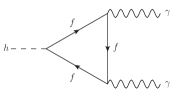
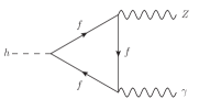
Figure 1: The Feynman diagrams with flavor-conserving vertices.

Table 1: The fermion representations in the minimal fermion extension model. The fermions are vector like, having both left- and right-handed components, therefore the model is automatically gauge anomaly free [22].

	$SU(3)_{c}$	$SU(2)$	$U(1)_{Y}$
$(f_{S}^{Y+1})_{L,R}$	${\bf 1}$	${\bf 1}$	$Y+1$
$(f_{D})_{L,R}$	${\bf 1}$	${\bf 2}$	$Y+1/2$
$(f_{S}^{Y})_{L,R}$	${\bf 1}$	${\bf 1}$	$Y$

II The model and its interactions

The new fermions can couple to the Higgs doublet $H$ and can also have bare masses. The Yukawa interaction and bare mass terms are given by

$${\cal L}_{H+M} = -m_{D}\overline{f}_{D}f_{D}-m_{S}^{Y}\overline{f}_{S}^{Y}f_{S}^{Y}-m_{S}^{Y+1}\overline{f}_{S}^{Y+1}f_{S}^{Y+1}-\left(c_{f}^{Y}\overline{f}_{D}f_{S}^{Y}\tilde{H}+c_{f}^{Y+1}\overline{f}_{D}f_{S}^{Y+1}H)+(\text{h.c.})\right),$$ (6)

where $\tilde{H}=i\tau_{2}H^{*}$. Here we have omitted parity-violating Yukawa terms of the form $\bar{f}\gamma_{5}f^{\prime}(H,\tilde{H})$ for simplicity, aiming to solve the $h\to Z\gamma$ excess problem.

The non-zero vev $v$ of Higgs can contribute to fermion masses leading to the new fermion mass matrices in the basis $(f^{X}_{D},f_{S}^{X})^{T}$ with $X=Y$ or $Y+1$ as the following

$$\hat{M}^{X}=\left(\begin{array}[]{cc}m_{D}&c_{f}^{X}v/\sqrt{2}\\ c_{f}^{X}v/\sqrt{2}&m_{S}^{X}\end{array}\right)\,.$$ (7)

The eigenstates $f^{X}=(f_{1}^{X},f_{2}^{X})^{T}$ of $\hat{M}^{X}$ read

$$\left(\begin{array}[]{c}f_{1}^{X}\\ f_{2}^{X}\end{array}\right)=\left(\begin{array}[]{cc}\cos\theta_{X}&\sin\theta_{X}\\ -\sin\theta_{X}&\cos\theta_{X}\end{array}\right)\left(\begin{array}[]{c}f_{D}^{X}\\ f_{S}^{X}\end{array}\right)\,,$$ (8)

where the eigenvalues and mixing angles are

$$m_{1,2}^{X} = \frac{m_{D}+m^{X}_{S}}{2}\pm\sqrt{\frac{(m_{D}-m^{X}_{S})^{2}}{4}+\frac{(c_{f}^{X})^{2}v^{2}}{2}}\,,~{}~{}~{}\sin 2\theta_{X}=\frac{\sqrt{2}c_{f}^{X}v}{m^{X}_{1}-m^{X}_{2}}\,.$$ (9)

In this basis, the mass and charge-conserved Lagrangian for $f^{X}$ are given as

$${\cal L}^{X}_{M} = -\left(m_{1}^{X}\overline{f}_{1}^{X}f_{1}^{X}+m_{2}^{X}\overline{f}_{2}^{X}f_{2}^{X}\right)\,,$$

$${\cal L}_{h}^{X} = -\frac{c_{f}^{X}h}{\sqrt{2}}\overline{f}^{X}\left(\sin 2\theta_{X}\sigma_{z}+\cos 2\theta_{X}\sigma_{x}\right)f^{X}\,,$$

$${\cal L}_{\gamma}^{X} = eX\overline{f}^{X}A^{\mu}\gamma_{\mu}f^{X}\,,$$ (10)

$${\cal L}_{Z}^{X} = e\overline{f}^{X}Z^{\mu}\gamma_{\mu}\left[-X\tan\theta_{W}-\frac{\eta_{X}}{4\cos\theta_{W}\sin\theta_{W}}\left(1+\cos 2\theta_{X}\sigma_{z}-\sin 2\theta_{X}\sigma_{x}\right)\right]f^{X}\,,$$

where $(\eta_{Y},\eta_{Y+1})=(1,-1)$ and $\sigma_{x,y,z}$ are the Pauli matrices operating in the $SU(2)_{L+R}$ rotational space of $f^{X}$. For example, $\overline{f}^{X}\sigma_{x}f^{X}=\overline{f}^{X}_{1}f^{X}_{2}+\overline{f}^{X}_{2}f^{X}_{1}$. On the other hand, the $W$-boson can induce a charge current given by

$${\cal L}_{W} = \frac{g}{\sqrt{2}}W^{+}_{\mu}\Big{(}\cos\theta_{Y+1}\cos\theta_{Y}\overline{f}_{1}^{Y+1}\gamma^{\mu}f_{1}^{Y}+\sin\theta_{Y+1}\sin\theta_{Y}\overline{f}_{2}^{Y+1}\gamma^{\mu}f_{2}^{Y}$$ (11)

$$- \cos\theta_{Y+1}\sin\theta_{Y}\overline{f}_{1}^{Y+1}\gamma^{\mu}f_{2}^{Y}-\cos\theta_{Y}\sin\theta_{Y+1}\overline{f}_{2}^{Y+1}\gamma^{\mu}f_{1}^{Y}\Big{)}+(\text{h.c.})\,.$$

As we will see shortly, to explain the data we need a large $Y$, which prohibits them to couple with the SM fermions. Hence, the Lagrangian remains invariant under the $U(1)$ rotation of $f_{1,2}^{Y,Y+1}\to e^{i\theta}f_{1,2}^{Y,Y+1}$, and at least one of the new fermions must be stable.

III Loop induced $h\to\gamma\gamma$ and $h\to Z\gamma$ in the model

We are ready to calculate the loop induced $h\to\gamma\gamma$ and $h\to Z\gamma$ in the minimally extended model described previously. The one loop diagrams inducing these decays are shown in Figures 1 and 2. There are two classes of diagrams, one shown in Figure 1 in which the fermions in the loop does not change identities which we refer as flavor-conserving ones, and the other as shown in Figure 2 in which the fermions in the loop change identities which we refer to as flavor-change diagrams. $h\to\gamma\gamma$ receives contributions from flavor-conserving class, and $h\to Z\gamma$ receive contributions from the both classes. These features make it possible to have NP contributions of the new fermions to $h\to\gamma\gamma$ and $h\to Z\gamma$ differently to addressing the problem we are dealing with.

Depending on the original parameters $m_{D}$, $m_{S}^{X}$ and $c_{f}^{X}$, there are three classes of possible mass eigenstates: 1. both $m_{1,2}^{X}$ are positive; 2. one of the $m^{X}_{1,2}$ is positive and the other negative; and 3. both $m^{X}_{1,2}$ are negative. In the last case, one can perform a chiral rotation $e^{i\gamma_{5}\pi/2}$ on the fields $f^{X}_{1,2}$ to make all masses positive and transform ${\cal L}_{h}\to-{\cal L}_{h}$, while leaving the other interaction terms unchanged. This would not change the final outcome comparing to the first case, as our final result depends on the value of $(c_{f}^{X})^{2}$. We therefore only need to consider the possibilities of 1. and 2. These two cases can have different features for $h\to\gamma\gamma$ and $h\to Z\gamma$. We proceed to discuss them in the following.

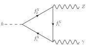
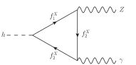
Figure 2: The Feynman diagrams with flavor-changing vertices

III.1 The case for $m^{X}_{1,2}$ both to be positive

The Feynman diagrams with flavor-conserving vertices are depicted in Figures 1 . The calculations are similar to that in the SM. The contributions with $f$ in the fermion loop are given as

$$\delta c_{Z}^{f}=Q_{f}g_{h}^{f}vg_{Z}^{f}\frac{1}{m_{f}}I_{Z}(\tau_{f},\lambda_{f})\,,~{}~{}~{}\delta c_{\gamma}^{f}=Q_{f}^{2}g^{f}_{h}v\frac{1}{m_{f}}A_{f}(\tau_{f})\,,$$ (12)

where $f\in\{f_{1}^{Y},f_{2}^{Y},f_{1}^{Y+1},f_{2}^{Y+1}\}$ and $\tau_{f}=m_{h}^{2}/4m_{f}^{2},~{}\lambda_{f}=m_{Z}^{2}/4m_{f}^{2}$. Here $Q_{f}$, $g_{h}^{f}$ and $g_{Z}^{f}$ are the coupling strengths of $A^{\mu}$, $h$ and $Z^{\mu}$ to $f$, where $Q_{f_{1,2}^{X}}=X$, $g_{h}^{f^{X}_{1}}=\sin 2\theta_{X}c_{f}^{X}h/\sqrt{2}$, $g_{h}^{f^{X}_{2}}=-\sin 2\theta_{X}c_{f}^{X}h/\sqrt{2}$, $g_{Z}^{f^{X}_{1}}=-(\eta_{X}(1+\cos 2\theta_{X})+4X\sin^{2}\theta_{W})/4\cos\theta_{W}\sin\theta_{W}$, and $g_{Z}^{f^{X}_{2}}=-(\eta_{X}(1-\cos 2\theta_{X})+4X\sin^{2}\theta_{W})/4\cos\theta_{W}\sin\theta_{W}$. The loop functions are given as

$$\begin{split}I_{Z}(a,b)&=\frac{2}{(a-b)}+\frac{2+2b-2a}{(b-a)^{2}}\,(f(b)-f(a))+\frac{4b}{(b-a)^{2}}\,(g(b)-g(a))\,,\\[4.26773pt] A_{f}(\tau)&=\frac{2}{\tau^{2}}\left[(\tau-1)f(\tau)+\tau\right]\,,\\ f(\tau)&=\left\{\begin{array}[]{lll}{\rm arcsin}^{2}\sqrt{\tau}&\tau\leq 1\\ -\frac{1}{4}\left(\log\frac{\sqrt{\tau}+\sqrt{\tau-1}}{\sqrt{\tau}-\sqrt{\tau-1}}-i\pi\right)^{2}&\tau>1\end{array}\right.\,,\\ g(\tau)&=\begin{cases}\sqrt{1/\tau-1}\,\arcsin(\sqrt{\tau})&\tau\leq 1\\[2.84544pt] \frac{1}{2}\sqrt{1-1/\tau}\left(\log\frac{\sqrt{\tau}+\sqrt{\tau-1}}{\sqrt{\tau}-\sqrt{\tau-1}}-i\pi\right)&\tau>1\end{cases}\,.\\ \end{split}$$ (13)

At $m_{f}\gg m_{h,Z}$, we have $I_{Z}(\tau_{f},\lambda_{f})=A_{f}(\tau_{f})=4/3$.

The Feynman diagrams with flavor-changing vertices are depicted in Figure 2. Due to the Ward identity, the photon vertices must conserve the flavor and hence this type of diagrams are absent in $h\to\gamma\gamma$. The contribution of the $f^{X}$ doublet to $\delta c_{Z}$ is

$$\delta c_{Z}^{f_{1}^{X}f^{X}_{2}} = vQ_{f}g_{h}^{f^{X}_{1}f^{X}_{2}}g_{Z}^{f_{1}^{X}f_{2}^{X}}L(m^{X}_{1},m^{X}_{2})\,,$$ (14)

with the loop function given as

$$L(m_{1},m_{2}) = 2\int^{1}_{0}dy\int^{1}_{0}ydx\frac{-m_{1}(2y+1)xy+2m_{1}x^{2}y^{2}+m_{1}+m_{2}xy(-2y+2xy+1)}{(1-xy)m_{1}^{2}+xym_{2}^{2}-xym_{h}^{2}+x^{2}y^{2}m_{h}^{2}+(m_{h}^{2}-m_{Z}^{2})xy(1-y)}$$ (15)

$$+ 2\int^{1}_{0}dy\int^{1}_{0}ydx\frac{m_{1}(2y-3)xy+m_{1}+m_{2}(2y-1)xy}{(1-xy)m_{1}^{2}+xym_{2}^{2}-(y-xy)(1-y+xy)m_{Z}^{2}-xy(1-y)m_{h}^{2}}$$

$$+ (m_{1}\leftrightarrow m_{2})\,.$$

The coupling strengths can be read off from Eq. (II) as $g_{h}^{f_{1}^{X}f^{X}_{2}}=c_{f}^{X}\cos 2\theta_{X}/\sqrt{2}$ and $g_{Z}^{f_{1}^{X}f_{2}^{X}}=\eta_{X}\sin 2\theta_{X}/(4\cos\theta_{W}\sin\theta_{W})$.

To have some ideas about how the new fermions affect the decays, let us examine a limiting case to see their effects. Since the new fermions are expected to be much heavier than the SM particles, it is safe to take the limit of $m_{h,Z}/m_{1,2}^{X}\to 0$. In this limit, we can drop $m_{Z}^{2}$ and $m_{h}^{2}$. We obtain

$$L(m_{1},m_{2})=\frac{2\left(m_{1}^{2}-4m_{1}m_{2}+m_{2}^{2}\right)}{(m_{1}-m_{2})^{2}(m_{1}+m_{2})}-\frac{4m_{1}m_{2}\left(m_{1}^{2}-m_{1}m_{2}+m_{2}^{2}\right)\log(m_{2}^{2}/m_{1}^{2})}{(m_{1}-m_{2})^{3}(m_{1}+m_{2})^{2}}\,.$$ (16)

Around $m_{1}=m_{2}$, we have

$$L(m_{1},m_{2}) = \frac{16}{3(m_{1}+m_{2})}+{\cal O}\left(\frac{(m_{1}-m_{2})^{2}}{(m_{1}+m_{2})^{3}}\right)\,.$$ (17)

The above leads

$$\delta c_{\gamma} = -\frac{4}{3}\left(Y^{2}\frac{\left(c_{f}^{Y}v\right)^{2}}{m_{1}^{Y}m_{2}^{Y}}+(Y+1)^{2}\frac{\left(c_{f}^{Y+1}v\right)^{2}}{m_{1}^{Y+1}m_{2}^{Y+1}}\right)\,,$$ (18)

$$\delta c_{Z} = \frac{4\sin\theta_{W}}{3\cos\theta_{W}}\left(Y^{2}\frac{\left(c_{f}^{Y}v\right)^{2}}{m_{1}^{Y}m_{2}^{Y}}+(Y+1)^{2}\frac{\left(c_{f}^{Y+1}v\right)^{2}}{m_{1}^{Y+1}m_{2}^{Y+1}}\right)+\frac{2}{3\sin\theta_{W}\cos\theta_{W}}\left(Y\frac{\left(c_{f}^{Y}v\right)^{2}}{m_{1}^{Y}m_{2}^{Y}}-(Y+1)\frac{\left(c_{f}^{Y+1}v\right)^{2}}{m_{1}^{Y+1}m_{2}^{Y+1}}\right),$$

around $|m_{1}^{X}|\approx|m_{2}^{X}|$. Therefore, for the case with $m_{1,2}^{X}>0$, we see that $\delta c_{\gamma}$ ($\delta c_{Z}$) constructively (destructively) interfere with $c_{\gamma}^{\text{SM}}$ ($c_{Z}^{\text{SM}}$), which would lead to $\mu_{\gamma}>1$ and $\mu_{Z}<1$ for $|\delta c_{\gamma,Z}|<|c_{\gamma,Z}^{\text{SM}}|$. This trend is maintained for even keeping finite $m_{h}$ and $m_{Z}$. Hence, the scenario of $m_{1,2}^{X}>0$ is not able to explain the observed discrepancy in the experiment.

III.2 The case for one of $m^{X}_{1,2}$ to be negative

From Eq. (18) we see that if setting $m_{2}^{Y+1}<0$, a destructive interference between the $f^{Y}$ and $f^{Y+1}$ doublets for $\delta c_{\gamma}$ can happen while leave the second term in $\delta c_{Z}$ to tune $c_{Z}$. To rigorously address the scenario with $m_{2}^{Y+1}<0$, a rotation of $f_{2}^{Y+1}\to\gamma_{5}f_{2}^{Y+1}$ is necessary to ensure the positiveness of the fermion mass. While ${\cal L}^{Y}_{M,h,\gamma,Z}$ remain unchanged, the others are modified to

$${\cal L}^{Y+1}_{M} = -m_{1}^{Y+1}\overline{f}_{1}^{Y+1}f_{1}^{Y+1}-|m_{2}^{Y+1}|\overline{f}_{2}^{Y+1}f_{2}^{Y+1}\,,$$

$${\cal L}_{h}^{Y+1} = -\frac{c_{f}^{Y+1}h}{\sqrt{2}}\overline{f}^{Y+1}\left(\sin 2\theta_{Y+1}+\cos 2\theta_{Y+1}i\sigma_{y}\gamma_{5}\right)f^{Y+1}\,,$$ (19)

$${\cal L}_{Z}^{Y+1} = e\overline{f}^{Y+1}Z^{\mu}\gamma_{\mu}\left[-(Y+1)\tan\theta_{W}-\frac{\eta_{Y+1}}{4\cos\theta_{W}\sin\theta_{W}}\left(\sigma_{z}+\cos 2\theta_{Y+1}-\sin 2\theta_{Y+1}\sigma_{x}\gamma_{5}\right)\right]f^{Y+1}\,,$$

$${\cal L}_{W} = \frac{g}{\sqrt{2}}W^{+}_{\mu}\Big{(}\cos\theta_{Y+1}\cos\theta_{Y}\overline{f}_{1}^{Y+1}\gamma^{\mu}f_{1}^{Y}+\sin\theta_{Y+1}\sin\theta_{Y}\overline{f}_{2}^{Y+1}\gamma^{\mu}\gamma_{5}f_{2}^{Y}$$

$$- \cos\theta_{Y+1}\sin\theta_{Y}\overline{f}_{1}^{Y+1}\gamma^{\mu}f_{2}^{Y}-\cos\theta_{Y}\sin\theta_{Y+1}\overline{f}_{2}^{Y+1}\gamma^{\mu}\gamma_{5}f_{1}^{Y}\Big{)}+(\text{h.c.})\,.$$

We have carried out detailed calculations and find that for $h\to\gamma\gamma$ and $h\to Z\gamma$, the consequences of this rotation can be effectively modeled by substituting $m_{2}^{Y+1}$ with $-m_{2}^{Y+1}$ in Eqs. (14), (15) and (18). It results in the favorable solution with $|\delta c_{\gamma}|<|c_{\gamma}^{\text{SM}}|.$

Before ending this section, we note that from Eq. (18) there is a second set of solutions with $m_{2}^{Y+1}<0$. By taking $c_{f}^{Y}=0$, $\delta c_{\gamma}$ and $c_{\gamma}^{\text{SM}}$ are opposite in sign and it is possible to explain the data with the feature of $\delta c_{\gamma}\approx-2c_{\gamma}^{\text{SM}}$. In this scenario, $f_{S}^{Y}$ decouples from the other fermions, and it is not necessary to include it in the model.

It is worth mentioning that Ref. [9] considered the fermions with the same representations as those in Table 2. In particular, by considering $m_{D},m_{S}^{Y,Y+1}\to 0$, we can reproduce the results in Ref. [9]. In this case, the only solution is where $\delta c_{\gamma}\approx-2c_{\gamma}^{\text{SM}}$ with $|Q_{f}|$ found to be $1e$ and $2e$. However, it is more natural to have a solution where $c^{\text{SM}}_{\gamma}\gg\delta c_{\gamma}$.

IV Numerical results

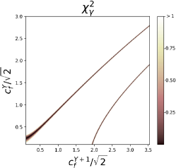
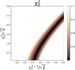
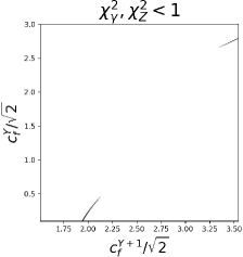
Figure 3: In Figures (a) and (b), the colored regions represent the parameter space consistent with $\mu_{\gamma}^{\text{exp}}$ and $\mu_{Z}^{\text{exp}}$ within one standard deviation, where the color indicates the values of $\chi^{2}_{\gamma,Z}$ as defined in Eq. (21). Figure (c) displays the regions that satisfy both $\chi_{\gamma}^{2}<1$ and $\chi_{Z}^{2}<1$. The upper and lower lines in Figures (a) and (c) denote the solutions where $|\delta c_{\gamma}|\ll|c_{\gamma}^{\text{SM}}|$ and $\delta c_{\gamma}\approx-2c_{\gamma}^{\text{SM}}$, respectively.

We now provide numerical results for the case with negative $m_{2}^{Y+1}$. For simplicity, we adopt $m_{D}=m_{S}^{Y}=-m_{S}^{Y+1}\,,$ and the masses are given by

$$m_{1,2}^{Y} = m_{D}\pm\frac{c_{f}^{Y}v}{\sqrt{2}}\,,~{}~{}~{}m_{1}^{Y+1}=-m_{2}^{Y+1}=\sqrt{m_{D}^{2}+\frac{(c_{f}^{Y+1}v)^{2}}{2}}\,.$$ (20)

Without loss of generality, we take $m_{1}^{Y}>m_{2}^{Y}$. Hence, we have the hierarchy of $m_{1}^{Y}>|m_{1,2}^{Y+1}|>m_{2}^{Y}$, making $f_{2}^{Y}$ being the stable particle due to the energy conservation. For a meaningful perturbative calculation, we consider only the regions where $(c_{f}^{X}/\sqrt{2})^{2}<4\pi$ and fix $Y=-9$. We also confine us to have the lightest new charged fermion mass to be larger than $1600$ GeV to satisfy the experimental lower bound for $|Q_{f}|$ up to 7 [23].

To find the regions of parameter which fit data well, we define

$$\chi_{\gamma}^{2}=\left(\frac{\mu^{\text{exp}}_{\gamma}-\mu_{\gamma}}{\sigma^{\text{exp}}_{\gamma}}\right)^{2}\,,~{}~{}\chi_{Z}^{2}=\left(\frac{\mu^{\text{exp}}_{Z}-\mu_{Z}}{\sigma^{\text{exp}}_{Z}}\right)^{2}\,,$$ (21)

where $\sigma^{\text{exp}}_{\gamma,Z}$ stand for the experimental uncertainties of $\mu_{\gamma,Z}$. In Figure 3(a), (b) and (c), we plot the allowed parameter spaces by setting $\chi_{\gamma}^{2}<1$, $\chi^{2}_{Z}<1$ and $\chi_{\gamma}^{2},\chi_{Z}^{2}<1$, respectively. From Figure 3(a) and (c), it is observed that there are two sets of solutions. We name the upper line Solution 1, characterized by $|\delta c_{\gamma}|\ll|c_{\gamma}^{\text{SM}}|$, while the lower line is named Solution 2, characterized by $\delta c_{\gamma}\approx-2c_{\gamma}^{\text{SM}}$, representing the solution mentioned at the end of the last section. For $\chi^{2}_{Z}$ depicted in Figure 3(b), there is only one set of solutions with $|\delta c_{Z}|<|c_{Z}^{\text{SM}}|$ in contrast. It is worth noting that, if we consider $m_{2}^{Y+1}>0$, there would be no solution here. In the limit of $m_{D}\gg c_{f}^{X}v$, the lines in Figure 3 exhibit a slope of $(Y+1)^{2}/Y^{2}$, necessary to achieve a cancellation between the $f^{Y}$ and $f^{Y+1}$ doublets in Eq. (18).

We also show in Figure 3 (c), the two sets of solutions with the smallest couplings. They are

$$\mbox{Solution 1}:\;\;\;\;\left(c_{f}^{Y+1},c_{f}^{Y}\right)_{\delta c_{\gamma}\approx 0}=\left(4.73,~{}3.80\right)\,,~{}~{}~{}$$

$$\mbox{Solution 2}:\;\;\;\;\left(c_{f}^{Y+1},c_{f}^{Y}\right)_{\delta c_{\gamma}\approx-2c_{\gamma}^{\text{SM}}}=(2.69,0)\,.$$ (22)

The corresponding predictions for other parameters are given by

Solution 1 $$: \;\;\left(\theta_{Y+1},\theta_{Y}\right)=(10^{\circ},45^{\circ}),\;\;\;\;\left(\mu_{\gamma},\mu_{Z}\right)=(1.10,1.55)$$

$$\;\;(m_{1}^{Y},m_{2}^{Y})=(2923,1600)~{}\text{GeV}\,,~{}~{}~{}~{}m_{1,2}^{Y+1}=2407~{}\text{GeV}\,,$$

Solution 2 $$: \;\;(\theta_{Y+1},\theta_{Y})=(8^{\circ},0^{\circ}),\;\;\;\;\left(\mu_{\gamma},\mu_{Z}\right)=(1.10,2.88)\,,$$ (23)

$$\;\;(m_{1}^{Y},m_{2}^{Y})=(1600,1600)~{}\text{GeV}\,,~{}~{}~{}~{}m_{1,2}^{Y+1}=1667~{}\text{GeV}\,.$$

respectively.

We therefore have found two classes of solutions which do not modify branching ratio for $h\to\gamma\gamma$, but enhance the branching ratio to the current averaged value. Solution 2 seems to be a contrived solution although cannot be ruled out simply using branching ratio measurements. If the current data are confirmed, we would think Solution 1 to be a better solution.

Before ending the discussion, we would like to comment on some phenomenological for the model at colliders. The new fermions in the model can be produced which has been discussed for smaller $|Y|$ and new fermion masses in Ref. [9]. Since in our model the hyper-charge $|Y|$ is large, the lightest new fermion is constrained to be larger than $1600$ GeV [23]. The production at the current LHC may be scarce or absent. However, with higher energies and higher luminosity, the new fermions in our model may be produced. The signature of the lightest fermion will leave a charge track in the detector to be measured. While to the heavier ones, if produced they can decay into other final states. For Solution 1, except for $f_{2}^{Y}$ the others will decay to $f_{2}^{Y}$ plus either a $W$-boson or $Z$-boson. But these decays will have large widths of the order of hundreds GeV, making detection difficult since there will not be a sharp resonance peak to look for. On the other hand, for Solution 2, the fermion mass differences are not high enough to form an on-shell gauge boson. They decay into an off-shell $W$-boson, which then decays into a charged lepton and a neutrino, with the decay widths being on the order of a few to a few tens of MeV. Similarly, the decay widths to light quark jet pairs are twice as large. Such measurements may provide information to distinguish between the two different solutions.

V Conclusion

We have studied some implications of the possible $h\to Z\gamma$ excess from recent measurements by ALTLAS and CMS. If this excess is confirmed, it is a signal of NP beyond SM. For NP contribution, while modifying $h\to Z\gamma$, in general it also can affect $h\to\gamma\gamma$. Since measured branching ratio for this process agrees with SM prediction well, therefore there are several constraints on theoretical models trying to simultaneously explain data on $h\to\gamma\gamma$ and $h\to Z\gamma$. We find that a minimally fermion singlets and doublet extended NP model can explain simultaneously the current data on these decays. There are two solutions. One is the SM amplitude $c_{Z}^{\text{SM}}$ is enhanced by $\delta c_{Z}$ for $h\to Z\gamma$ to the observed value, but the $h\to\gamma\gamma$ amplitude $c_{\gamma}^{\text{SM}}+\delta c_{\gamma}$ is decreased to $-c_{\gamma}^{\text{SM}}$ to give the observed branching ratio. This seems to be a contrived solution that although cannot be ruled out simply using branching ratio measurements. We, however, have found another solution which naturally enhances the $h\to Z\gamma$ to the measured value, but keeps the $h\to\gamma\gamma$ close to its SM prediction. With high energy colliders which can produce these new heavy fermions, by studying the decay pattens of the heavy fermions, it is possible to distinguish the two solutions we found. We eagerly await future data to provide more information.

References

• [1] G. Aad et al. [ATLAS], Phys. Lett. B 716, 1-29 (2012) [arXiv:1207.7214 [hep-ex]].
• [2] S. Chatrchyan et al. [CMS], Phys. Lett. B 716, 30-61 (2012) [arXiv:1207.7235 [hep-ex]].
• [3] R. N. Cahn, M. S. Chanowitz and N. Fleishon, Phys. Lett. B 82, 113-116 (1979).
• [4] L. Bergstrom and G. Hulth, Nucl. Phys. B 259, 137-155 (1985) [erratum: Nucl. Phys. B 276, 744-744 (1986)].
• [5] [CMS], CMS-PAS-HIG-13-005.
• [6] G. Aad et al. [ATLAS], Phys. Lett. B 726, 88-119 (2013) [erratum: Phys. Lett. B 734, 406-406 (2014)] [arXiv:1307.1427 [hep-ex]].
• [7] N. Bizot and M. Frigerio, JHEP 01, 036 (2016) [arXiv:1508.01645 [hep-ph]].
• [8] Q. H. Cao, L. X. Xu, B. Yan and S. H. Zhu, Phys. Lett. B 789, 233-237 (2019) [arXiv:1810.07661 [hep-ph]].
• [9] D. Barducci, L. Di Luzio, M. Nardecchia and C. Toni, JHEP 12, 154 (2023) [arXiv:2311.10130 [hep-ph]].
• [10] G. Lichtenstein, M. A. Schmidt, G. Valencia and R. R. Volkas, [arXiv:2312.09409 [hep-ph]].
• [11] T. T. Hong, V. K. Le, L. T. T. Phuong, N. C. Hoi, N. T. K. Ngan and N. H. T. Nha, [arXiv:2312.11045 [hep-ph]].
• [12] R. Boto, D. Das, J. C. Romao, I. Saha and J. P. Silva, [arXiv:2312.13050 [hep-ph]].
• [13] N. Das, T. Jha and D. Nanda, [arXiv:2402.01317 [hep-ph]].
• [14] K. Cheung and C. J. Ouseph, [arXiv:2402.05678 [hep-ph]].
• [15] A. Tumasyan et al. [CMS], JHEP 05, 233 (2023) [arXiv:2204.12945 [hep-ex]].
• [16] G. Aad et al. [ATLAS and CMS], Phys. Rev. Lett. 132, 021803 (2024) [arXiv:2309.03501 [hep-ex]].
• [17] [ATLAS], ATLAS-CONF-2019-029.
• [18] A. M. Sirunyan et al. [CMS], JHEP 07, 027 (2021) [arXiv:2103.06956 [hep-ex]].
• [19] A. Djouadi, Phys. Rept. 457, 1-216 (2008) [arXiv:hep-ph/0503172 [hep-ph]].
• [20] A. Y. Korchin and V. A. Kovalchuk, Phys. Rev. D 88, no.3, 036009 (2013) [arXiv:1303.0365 [hep-ph]].
• [21] G. Aad et al. [ATLAS], Nature 607, no.7917, 52-59 (2022) [erratum: Nature 612, no.7941, E24 (2022)] [arXiv:2207.00092 [hep-ex]].
• [22] Q. Bonnefoy, L. Di Luzio, C. Grojean, A. Paul and A. N. Rossia, JHEP 07, 189 (2021) [arXiv:2011.10025 [hep-ph]].
• [23] G. Aad et al. [ATLAS], Phys. Lett. B 847, 138316 (2023) [arXiv:2303.13613 [hep-ex]].