Variational Continual Test-Time Adaptation

Abstract

The prior drift is crucial in Continual Test-Time Adaptation (CTTA) methods that only use unlabeled test data, as it can cause significant error propagation. In this paper, we introduce VCoTTA, a variational Bayesian approach to measure uncertainties in CTTA. At the source stage, we transform a pre-trained deterministic model into a Bayesian Neural Network (BNN) via a variational warm-up strategy, injecting uncertainties into the model. During the testing time, we employ a mean-teacher update strategy using variational inference for the student model and exponential moving average for the teacher model. Our novel approach updates the student model by combining priors from both the source and teacher models. The evidence lower bound is formulated as the cross-entropy between the student and teacher models, along with the Kullback-Leibler (KL) divergence of the prior mixture. Experimental results on three datasets demonstrate the method’s effectiveness in mitigating prior drift within the CTTA framework.

1 Introduction

Continual Test-Time Adaptation (CTTA) (Wang et al., 2022) aims to enable a model to accommodate a sequence of distinct distribution shifts during the testing time (See Fig. 1(a)), making it applicable to various risk-sensitive applications in open environments, such as autonomous driving and medical imaging. However, real-world non-stationary test data exhibit high uncertainty in their temporal dynamics (Huang et al., 2022), presenting challenges related to error accumulation (Wang et al., 2022). Previous CTTA studies rely on methods that enforce prediction confidence, such as entropy minimization. However, these approaches often lead to predictions that are overly confident and less well-calibrated, thus limiting the model’s ability to quantify risks during predictions. The reliable estimation of uncertainty becomes particularly crucial in the context of continual distribution shift (Ovadia et al., 2019). Therefore, it is meaningful to design a model capable of encoding the uncertainty associated with temporal dynamics and effectively handling distribution shifts. The objective of this paper is to devise a test-time adaptation procedure that not only enhances predictive accuracy under distribution shifts but also provides reliable uncertainty estimates.

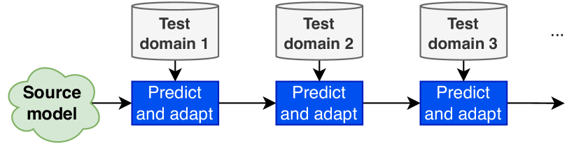
(a) CTTA task

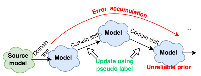
(b) Unreliable prior in CTTA

Figure 1: A CTTA model is updated using pseudo labels, which may result in error accumulations and make the prior unreliable.

To address the above problem, we refer to the Bayesian Inference (BI) approach (Box & Tiao, 2011), which retains a distribution over model parameters that indicates the plausibility of different settings given the observed data, and it has been witnessed as effective in traditional continual learning tasks (Nguyen et al., 2018). In Bayesian continual learning, the posterior in the last learning task is set to be the current prior which will be multiplied by the current likelihood. This kind of prior transmission is designed to reduce catastrophic forgetting in continual learning (Liu et al., ; Sun et al., 2022; Du et al., 2023; Lyu et al., 2023, 2021). However, this is not feasible in CTTA because unlabeled data may introduce significant prior drift. That is, as shown in Fig. 1(b), an unreliable prior may lead to a poor posterior, which may then propagate errors to the next inference, leading to the accumulation of errors.

Thus, we delve into mitigating prior drift in CTTA within a BI framework in this paper. To approximate the intractable likelihood in Bayesian inference, we adopt to use online Variational Inference (VI) (Wang et al., 2011; Sato, 2001), and accordingly name our method Variational Continual Test-Time Adaptation (VCoTTA). At the source stage, we first transform a pretrained deterministic model into a Bayesian Neural Network (BNN) by a variational warm-up strategy, where the local reparameterization trick (Kingma et al., 2015) is used to inject uncertainties into the source model. During the testing phase, we employ a mean-teacher update strategy, where the student model is updated via VI and the teacher model is updated by the exponential moving average. Specifically, for the update of the student model, we propose to use a mixture of priors from both the source and teacher models, then the Evidence Lower BOund (ELBO) becomes the cross-entropy between the student and teachers plus the KL divergence of the prior mixture. We demonstrate the effectiveness of the proposed method on three datasets, and the results show that the proposed method can mitigate the prior drift in CTTA and obtain clear performance improvements.

Our contributions are three-fold:

1. This paper develops VCoTTA, a simple yet general framework for continual test-time adaptation that leverages online VI within BNN.

2. We propose to transform an off-the-shelf model into a BNN via a variational warm-up strategy, which injects uncertainties into the model.

3. We build a mean-teacher structure for CTTA, and propose a strategy to blend the teacher’s prior with the source’s prior to mitigate prior drift.

2 Related Work

2.1 Continual Test-Time Adaptation

Test-Time Adaptation (TTA) enables the model to dynamically adjust to the characteristics of the test data, i.e. target domain, in a source-free and online manner (Jain & Learned-Miller, 2011; Sun et al., 2020; Wang et al., 2020). Previous works have enhanced TTA performance through the designs of unsupervised loss (Mummadi et al., 2021; Zhang et al., 2022; Liu et al., 2021; Choi et al., 2022; Chen et al., 2022; Gandelsman et al., 2022). These endeavours primarily focus on enhancing adaptation within a fixed target domain, representing a single-domain TTA setup. In this scenario, the model adapts to a specific target domain and then resets to its original pre-trained state with the source domain, prepared for the next target domain adaptation.

Recently, CTTA (Wang et al., 2022) has been introduced to tackle TTA within a continuously changing target domain, involving long-term adaptation. This configuration often grapples with the challenge of error accumulation (Tarvainen & Valpola, 2017; Wang et al., 2022). Specifically, prolonged exposure to unsupervised loss from unlabeled test data during long-term adaptation may result in significant error accumulation. Additionally, as the model is intent on learning new knowledge, it is prone to forgetting source knowledge, which poses challenges when accurately classifying test samples similar to the source distribution.

To solve the two challenges, the majority of the existing methods focus on improving the confidence of the source model during the testing phase. These methods employ the mean-teacher architecture (Tarvainen & Valpola, 2017) to mitigate error accumulation, where the student learns to align with the teacher and the teacher updates via moving average with the student. As to the challenge of forgetting source knowledge, some methods adopt augmentation-averaged predictions (Wang et al., 2022; Brahma & Rai, 2023; Döbler et al., 2023; Yang et al., 2023) for the teacher model, strengthening the teacher’s confidence to reduce the influence from highly out-of-distribution samples. Some methods, such as Döbler et al. (2023); Chakrabarty et al. (2023), propose to adopt the contrastive loss to maintain the already learnt semantic information. Some methods believe that the source model is more reliable, thus they are designed to restore the source parameters (Wang et al., 2022; Brahma & Rai, 2023). Though the above methods keep the model from confusion of vague pseudo labels, they may suffer from overly confident predictions that are less calibrated. To mitigate this issue, it is helpful to estimate the uncertainty in the neural network.

2.2 Bayesian Neural Network

Bayesian framework is natural to incorporate past knowledge and sequentially update the belief with new data (Zhao et al., 2022). The bulk of work on Bayesian deep learning has focused on scalable approximate inference methods. These methods include stochastic VI (Hernández-Lobato & Adams, 2015; Louizos & Welling, 2017), dropout (Gal & Ghahramani, 2016; Kingma et al., 2015) and Laplace approximation (Ritter et al., 2018; Friston et al., 2007) etc., and leveraging the stochastic gradient descent (SGD) trajectory, either for a deterministic approximation or sampling. In a BNN, we specify a prior $p(\boldsymbol{\theta})$ over the neural network parameters, and compute the posterior distribution over parameters conditioned on training data, $p(\boldsymbol{\theta}|\mathcal{D})\propto p(\boldsymbol{\theta})p(\mathcal{D}|\boldsymbol{\theta})$. This procedure should give considerable advantages for reasoning about predictive uncertainty, which is especially relevant in the small-data setting.

Crucially, when performing Bayesian inference, we need to choose a prior distribution that accurately reflects the prior beliefs about the model parameters before seeing any data (Gelman et al., 1995; Fortuin et al., 2021). In conventional static machine learning, the most common choice for the prior distribution over the BNN weights is the simplest one: the isotropic Gaussian distribution. However, this choice has been proved indeed suboptimal for BNNs (Fortuin et al., 2021). Recently, some studies estimate uncertainty in continual learning within a BNN framework, such as Nguyen et al. (2018); Ebrahimi et al. (2019); Farquhar & Gal (2019); Kurle et al. (2019). They set the current prior to the previous posterior to mitigate catastrophic forgetting. However, the prior transmission is not reliable in the unsupervised CTTA task. Any prior mistakes will be enlarged by adaptation progress, manifesting error accumulation, which can be seen in Fig. 2. To solve the prior drift problem, in this paper, we propose a prior mixture method based on VI.

3 Variational CTTA

We start from the BI in typical continual learning, where the model aims to learn multiple classification tasks in sequence. Let $\mathcal{D}=\{(x_{n},y_{n})\}_{n=1}^{N}$ be the training set, where $x_{n}$ and $y_{n}$ denotes the training sample and the corresponding class label. The task $t$ is to learn a direct posterior approximation over the model parameter $\boldsymbol{\theta}$ as follows.

$$p(\boldsymbol{\theta}|\mathcal{D}_{1:t})~{}\propto~{}p_{t}(\boldsymbol{\theta})p(\mathcal{D}_{t}|\boldsymbol{\theta}),$$ (1)

where $p(\boldsymbol{\theta}|\mathcal{D}_{1:t})$ denotes the posterior of sequential tasks on the learned parameter and $p(\mathcal{D}_{t}|\boldsymbol{\theta})$ is the likelihood of the current task. The current prior $p_{t}(\boldsymbol{\theta})$ is regarded as the given knowledge. Nguyen et al. (2018) propose that this current prior can be the posterior learned in the last task, i.e., $p_{t}(\boldsymbol{\theta})=p(\boldsymbol{\theta}|\mathcal{D}_{1:t-1})$, thus the inference becomes

$$p(\boldsymbol{\theta}|\mathcal{D}_{1:t})~{}\propto~{}p(\boldsymbol{\theta}|\mathcal{D}_{1:t-1})p(\mathcal{D}_{t}|\boldsymbol{\theta}).$$ (2)

This process can be shown in Fig. 2(a).

In contrast to continual learning, CTTA faces a sequence of learning tasks in test time without any label information, requiring the model to adapt to each novel domain sequentially. The CTTA model is first trained on a source dataset $\mathcal{D}_{0}$, and then adapted to unlabeled test domains starting from $\mathcal{U}_{1}$. For the $t$-th adaptation, we have

$$p(\boldsymbol{\theta}|\mathcal{U}_{1:t}\cup\mathcal{D}_{0})\propto p_{t}(\boldsymbol{\theta})p(\mathcal{U}_{t}|\boldsymbol{\theta}).$$ (3)

Similarly, we can set the last posterior to be the current prior, i.e., $p_{t}(\boldsymbol{\theta})=p(\boldsymbol{\theta}|\mathcal{U}_{1:t-1}\cup\mathcal{D}_{0})$ and $p_{1}(\boldsymbol{\theta})=p(\boldsymbol{\theta}|\mathcal{D}_{0})$. However, the adaption with the unlabeled test data will cause significant error accumulation. In other words, an unreliable prior $p_{t}(\boldsymbol{\theta})$ will make the current posterior even less trustworthy. Moreover, the joint likelihood $p(\mathcal{U}_{t}|\boldsymbol{\theta})$ for $t>0$ is intractable on unlabeled data.

To make Bayesian inference feasible, in this paper, we transform the question to an easy-to-compute form. Referring to Grandvalet & Bengio (2004), the unsupervised inference can be transformed into

$$p(\boldsymbol{\theta}|\mathcal{U})\propto p(\boldsymbol{\theta})\exp\left(-{\lambda}{H}(\mathcal{U}|\boldsymbol{\theta})\right),$$ (4)

where $H$ denotes the conditional entropy and $\lambda$ is a scalar hyperparameter to weigh the entropy term. This simple form reveals that the prior belief about the conditional entropy of labels is given by the inputs. The observation of unlabeled test inputs $\mathcal{U}$ provides information on the drift of the input distribution, which can be used to update the belief over the learned parameters $\boldsymbol{\theta}$ through Eq. (4). Consequently, this allows the utilization of unlabeled data for Bayesian inference. More detailed derivations can be seen in Appendix A.

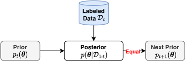
(a) BI in continual learning

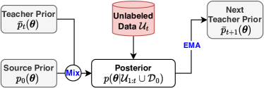
(b) BI in CTTA

Figure 2: Bayesian inference comparison between continual learning and CTTA. We find the traditional prior transmission is infeasible in CTTA because of the prior shift from unlabeled data. In our method, we place CTTA in a mean-teacher structure, and design BI in CTTA using a mixture of teacher prior and source prior. The next teacher prior is updated by the exponential moving average.

In a BNN, the posterior distribution is often intractable and some approximation methods are required, even when calculating the initial posterior. In this paper, we leverage online VI, as it typically outperforms the other methods for complex models in the static setting (Bui et al., 2016). VI defines a variational distribution $q(\boldsymbol{\theta})$ to approxmiate the posterior $p(\boldsymbol{\theta}|\mathcal{U})$. The approximation process is as follows.

$$q_{t}(\boldsymbol{\theta})=\arg\min_{q\in\mathbb{Q}}\mathrm{KL}\left[q(\boldsymbol{\theta})\parallel\frac{1}{Z_{t}}p_{t}(\boldsymbol{\theta})e^{-{\lambda}{H}(\mathcal{U}_{t}|\boldsymbol{\theta})}\right],$$ (5)

where $\mathbb{Q}$ is the distribution searching space and $Z_{t}$ is the intractable normalizing hyperparameter. Thus, referring to Appendix B, the ELBO is computed by

$${\text{ELBO}}=-\lambda\mathbb{E}_{\boldsymbol{\theta}\sim q(\boldsymbol{\theta})}H(\mathcal{U}_{t}|\boldsymbol{\theta})-\text{KL}\left(q(\boldsymbol{\theta})||p_{t}(\boldsymbol{\theta})\right).$$ (6)

Optimizing with Eq. (6) may still suffer from large error accumulation. The entropy term may result in overly confident predictions that are less calibrated, while the KL term may be affected by an unreliable prior. In the following section, we will discuss how to solve the problems when computing the two terms.

4 Adaptation and Inference in VCoTTA

4.1 Mean-Teacher architecture

In the above section, we introduce the VI in CTTA but challenges remain, i.e., the prior drift. To mitigate the challenge, we adopt a Mean-Teacher (MT) structure (Tarvainen & Valpola, 2017) in the Bayesian inference process. MT is initially proposed in semi-supervised and unsupervised learning, where the teacher model guides the unlabeled data, helping the model generalize and improve performance with the utilization of large-scale unlabeled data.

MT structure is composed of a student model and a teacher model, where the student model learns from the teacher and the teacher updates using Exponential Moving Average (EMA) (Hunter, 1986). In this work, the student is set to be the variational distribution $q(\boldsymbol{\theta})$, which is a Gaussian mean-field approximation for its simplicity. It is achieved by stacking the biases and weights of the network as follows.

$$q(\boldsymbol{\theta})=\prod\nolimits_{d}\mathcal{N}\left(\boldsymbol{\theta}_{d};\mu_{d},\text{diag}(\sigma_{d}^{2})\right),$$ (7)

where $d$ denotes each dimension of the parameter. The teacher model $\bar{p}(\boldsymbol{\theta})$ is also a Gaussian distribution. Thus, the student model is updated by aligning it with the teacher model through the use of a cross-entropy (CE) loss

$$L_{\text{CE}}(q,\bar{p})=-\mathbb{E}_{\boldsymbol{\theta}\sim q(\boldsymbol{\theta})}\bar{p}(\mathcal{U}|\boldsymbol{\theta})\log q(\mathcal{U}|\boldsymbol{\theta}).$$ (8)

In our implementation, we also try to use Symmetric Cross-Entropy (SCE) (Wang et al., 2019) in CTTA,

$$L_{\text{SCE}}(q,\bar{p})=-\mathbb{E}_{\boldsymbol{\theta}\sim q(\boldsymbol{\theta})}\big{[}\bar{p}(\mathcal{U}|\boldsymbol{\theta})\log q(\mathcal{U}|\boldsymbol{\theta})$$ (9)

$$+q(\mathcal{U}|\boldsymbol{\theta})\log\bar{p}(\mathcal{U}|\boldsymbol{\theta})\big{]}.$$

SCE keeps the gradient for high and low confidence balanced, benefiting the optimization in unsupervised learning.

4.2 Mixture-of-Gaussian Prior

For the KL term, to reduce prior drift in unsupervised testing time, we propose a mixing-up approach to combining the teacher and source prior adaptatively. The source prior is warmed up upon the pretrained deterministic model $p_{1}(\boldsymbol{\theta})=p(\boldsymbol{\theta}|\mathcal{D}_{0})$ (see Sec. 4.3.1). The teacher model $\bar{p}_{t}(\boldsymbol{\theta})$ is updated by EMA (see Sec. 4.3.3). We assume that the prior should be the mixture of the two Gaussian priors. Using only the source prior, the adaptation is limited. While using only the teacher prior, the prior is prone to drift.

We use the mean entropy derived from a given serious data augmentation to represent the confidence of the two prior models, and mix up the two priors with a modulating factor

$$\alpha=\frac{1}{|\mathcal{I}|}\sum\nolimits_{i\in\mathcal{I}}\frac{e^{H(\mathcal{U}_{i}|\boldsymbol{\theta}_{0})/\tau}}{e^{H(\mathcal{U}_{i}|\boldsymbol{\theta}_{0})/\tau}+e^{H(\mathcal{U}_{i}|\bar{\boldsymbol{\theta}})/\tau}},$$ (10)

where $\mathcal{I}$ denotes augmentation types. $\boldsymbol{\theta}_{0}$ and $\bar{\boldsymbol{\theta}}$ are the parameters of the source model and the teacher model. $\tau$ means the temperature factor. Thus, as shown in Fig. 2(b), the current prior $p_{t}(\boldsymbol{\theta})$ is set to the mixture of priors as

$$p_{t}(\boldsymbol{\theta})=\alpha\cdot p_{1}(\boldsymbol{\theta})+(1-\alpha)\cdot\bar{p}_{t}(\boldsymbol{\theta}).$$ (11)

In the VI, we use the upper bound to update the KL term (Liu et al., 2019) (see Appendix C) for simplicity,

$$\text{KL}\left(q||p_{t}\right)\leq\alpha\cdot\text{KL}\left(q||{p}_{0}\right)+(1-\alpha)\cdot\text{KL}\left(q||\bar{p}_{t}\right).$$ (12)

Furthermore, we also improve the teacher-student alignment in the entropy term (see Eq. (9)) by picking up the augmented logits with a larger confidence than the raw data. That is, we replace the teacher log-likelihood $\log\bar{p}(x|\boldsymbol{\theta})$ by

$$\log{\bar{p}^{\prime}(x|\boldsymbol{\theta})}=\frac{\sum_{i\in\mathcal{I}}\mathbf{1}\left(f(\bar{p}(x^{\prime}_{i}))>f(\bar{p}(x))+\epsilon\right)\cdot\log\bar{p}(x^{\prime}_{i})}{\sum_{i\in\mathcal{I}}\mathbf{1}\left(f(\bar{p}(x^{\prime}_{i}))>f(\bar{p}(x))+\epsilon\right)},$$ (13)

where, for brevity, we let $\bar{p}(x^{\prime}_{i})=\bar{p}(x^{\prime}_{i}|\boldsymbol{\theta})$ and $\bar{p}(x)=\bar{p}(x)|\boldsymbol{\theta})$ in short. $f(\cdot)$ is the confidence function. $\epsilon$ denotes the confidence margin and $\mathbf{1}(\cdot)$ is an indicator function. Eq. (13) means that the reliable teacher is represented by the average of its augmentations with $\epsilon$ more confidence.

Algorithm 1 Variational warm-up

  Input: Source data $\mathcal{D}_{0}$, pretrained model $p_{0}(\boldsymbol{\theta})$

  Initialize prior distribution $p(\boldsymbol{\theta})$ with $p_{0}(\boldsymbol{\theta})$

  Update $p(\boldsymbol{\theta}|\mathcal{D}_{0})\approx q_{0}(\boldsymbol{\theta})$ by $p(\boldsymbol{\theta})$ and $\mathcal{D}_{0}$ using Eq. (14)

  Output: Source prior $p_{1}(\boldsymbol{\theta})=p(\boldsymbol{\theta}|\mathcal{D}_{0})$

4.3 Adaptation and Inference

4.3.1 Variational Warm-up

To obtain a source BNN, we choose not to train a model on the source data $\mathcal{D}_{0}$ from scratch. Warm-up has been used in CTTA to further build knowledge structure for the source model (Döbler et al., 2023; Brahma & Rai, 2023). Inspired by this, we design to transform the pretrained deterministic model to a BNN by variational warm-up. Specifically, we leverage the local reparameterization trick (Kingma et al., 2015) to add stochastic parameters, and warm up the model:

$$q_{0}(\boldsymbol{\theta})=\arg\min_{q\in\mathbb{Q}}\mathrm{KL}\left[q(\boldsymbol{\theta})\parallel\frac{1}{Z_{0}}p(\boldsymbol{\theta})p(\mathcal{D}_{0}|\boldsymbol{\theta})\right],$$ (14)

where $p(\boldsymbol{\theta})$ represents the prior distribution, say the pretrained deterministic model. By the variational warm-up, we can easily transform an off-the-shelf pretrained model into a BNN with a stochastic dynamic. The variational warm-up strategy is outlined in Algorithm 1.

Algorithm 2 Variational CTTA

  Input: Source data $\mathcal{D}_{0}$, pretrained model $p_{0}(\boldsymbol{\theta})$, Unlabeled test data from different domain $\mathcal{U}_{1:T}$

  $p_{1}(\boldsymbol{\theta})=\text{Variational warm-up}(\mathcal{D}_{0},p_{0}(\boldsymbol{\theta}))$. // Alg. 1

  for Domain shift $t=1$ to $T$ do

     for Test data $x\sim\mathcal{U}_{t}$ do

        Model predict for $x$ (Eq. (17))

        Update student model using $x$ (Eq. (15))

        Update teacher model via EMA (Eq. (16))

     end for

  end for

Table 1: Classification error rate (%) for the standard CIFAR10-to-CIFAR10C continual test-time adaptation task. All results are evaluated with the largest corruption severity level 5 in an online fashion.

Method	C1	C2	C3	C4	C5	C6	C7	C8	C9	C10	C11	C12	C13	C14	C15	Avg
Source	72.3	65.7	72.9	46.9	54.3	34.8	42.0	25.1	41.3	26.0	9.3	46.7	26.6	58.5	30.3	43.5
BN	28.1	26.1	36.3	12.8	35.3	14.2	12.1	17.3	17.4	15.3	8.4	12.6	23.8	19.7	27.3	20.4
Tent (Wang et al., 2020)	24.8	20.6	28.5	15.1	31.7	17.0	15.6	18.3	18.3	18.1	11.0	16.8	23.9	18.6	23.9	20.1
CoTTA (Wang et al., 2022)	24.5	21.5	25.9	12.0	27.7	12.2	10.7	15.0	14.1	12.7	7.6	11.0	18.5	13.6	17.7	16.3
PETAL (Brahma & Rai, 2023)	23.7	21.4	26.3	11.8	28.8	12.4	10.4	14.8	13.9	12.6	7.4	10.6	18.3	13.1	17.1	16.2
SATA (Chakrabarty et al., 2023)	23.9	20.1	28.0	11.6	27.4	12.6	10.2	14.1	13.2	12.2	7.4	10.3	19.1	13.3	18.5	16.1
SWA (Yang et al., 2023)	23.9	20.5	24.5	11.2	26.3	11.8	10.1	14.0	12.7	11.5	7.6	9.5	17.6	12.0	15.8	15.3
VCoTTA (Ours)	18.1	14.9	22.0	9.7	22.6	11.0	9.5	11.4	10.6	10.5	6.5	9.4	15.6	11.0	14.5	13.1

4.3.2 Student update

The student model $q_{t}(\boldsymbol{\theta})$ is adapted and approximated by VI in Eq. (5), the total process can be optimized by minimizing

$$L(q_{t}) =L_{\text{SCE}}(q_{t},\bar{p}^{\prime}_{t})$$ (15)

$$+\alpha\cdot\text{KL}\left(q_{t}||q_{0}\right)+(1-\alpha)\cdot\text{KL}\left(q_{t}||\bar{q}_{t}\right),$$

where $\bar{p}^{\prime}_{t}$ is the current augmented teacher model in Eq. (13), and $p_{1}(\boldsymbol{\theta})\approx q_{0}(\boldsymbol{\theta})$, $\bar{p}_{t}(\boldsymbol{\theta})\approx\bar{q}_{t}(\boldsymbol{\theta})$. The KL term between two Gaussians can be computed in a closed form.

4.3.3 Teacher update via EMA

The teacher model is updated by EMA. Let $(\boldsymbol{\mu},\boldsymbol{\sigma})$ and $(\bar{\boldsymbol{\mu}},\bar{\boldsymbol{\sigma}})$ be the mean and standard deviation (std) of the student and teacher model, respectively. At test time, the teacher model $\bar{q}_{t}(\boldsymbol{\theta})$ is updated in real-time by

$$\bar{\boldsymbol{\mu}}\leftarrow\beta\bar{\boldsymbol{\mu}}+(1-\beta)\boldsymbol{\mu},\quad\bar{\boldsymbol{\sigma}}\leftarrow\beta\bar{\boldsymbol{\sigma}}+(1-\beta)\boldsymbol{\sigma}.$$ (16)

Although the std is not used in the cross entropy to compute the likelihood, the teacher prior distribution is important to adjust the student distribution via the KL term.

4.3.4 Model inference

At any time, CTTA model needs to predict and adapt to the unlabeled test data. In our VCoTTA, we also use the mixed prior to serve as the inference model. That is, for a test data point $x$, the model inference is represented by

$$p_{t}(x) =\int p(x|\boldsymbol{\theta})p_{t}(\boldsymbol{\theta})d\boldsymbol{\theta}$$ (17)

$$=\int\alpha p(x|\boldsymbol{\theta})p_{1}(\boldsymbol{\theta})+(1-\alpha)p(x|\boldsymbol{\theta})\bar{p}_{t}(\boldsymbol{\theta})d\boldsymbol{\theta},$$

For the data prediction, the model only uses the expectation to reduce the stochastic, but leverages stochastic dynamics in domain adaptation.

4.3.5 The algorithm

We illustrate the whole algorithm in Algorithm 2. We first transform an off-the-shelf pretrained model into BNN via the variational warm-up strategy (Sec. 4.3.1). After that, we obtain a BNN, and for each domain shift, we forward and adapt each test data point in an MT architecture. For a data point $x$, we first predict the class label using the mixture of the source model and the teacher model (Sec. 4.3.4). Then, we update the student model using VI, where we use cross entropy to compute the entropy term and use the mixture of priors for the KL term (Sec. 4.3.2). Finally, we update the BNN teacher model via EMA (Sec. 4.3.3). See more details in Appendix D. The process is feasible for any test data without labels.

Table 2: Classification error rate (%) for the standard CIFAR100-to-CIFAR100C continual test-time adaptation task. All results are evaluated with the largest corruption severity level 5 in an online fashion. C1 to C15 are 15 corruptions for the datasets (see Sec. 5.1).

Method	C1	C2	C3	C4	C5	C6	C7	C8	C9	C10	C11	C12	C13	C14	C15	Avg
Source	73.0	68.0	39.4	29.3	54.1	30.8	28.8	39.5	45.8	50.3	29.5	55.1	37.2	74.7	41.2	46.4
BN	42.1	40.7	42.7	27.6	41.9	29.7	27.9	34.9	35	41.5	26.5	30.3	35.7	32.9	41.2	35.4
Tent (Wang et al., 2020)	37.2	35.8	41.7	37.9	51.2	48.3	48.5	58.4	63.7	71.1	70.4	82.3	88.0	88.5	90.4	60.9
CoTTA (Wang et al., 2022)	40.1	37.7	39.7	26.9	38.0	27.9	26.4	32.8	31.8	40.3	24.7	26.9	32.5	28.3	33.5	32.5
PETAL (Brahma & Rai, 2023)	38.3	36.4	38.6	25.9	36.8	27.3	25.4	32.0	30.8	38.7	24.4	26.4	31.5	26.9	32.5	31.5
SATA (Chakrabarty et al., 2023)	36.5	33.1	35.1	25.9	34.9	27.7	25.4	29.5	29.9	33.1	23.6	26.7	31.9	27.5	35.2	30.3
SWA (Yang et al., 2023)	39.4	36.4	37.4	25.0	36.0	26.6	25.0	29.1	28.4	35.0	23.5	25.1	28.5	25.8	29.6	30.0
VCoTTA (Ours)	35.3	32.8	38.9	23.8	34.6	25.5	23.2	27.5	26.7	30.4	22.1	23.0	28.1	24.2	30.4	28.4

Table 3: Classification error rate (%) for the standard ImageNet-to-ImageNetC continual test-time adaptation task. All results are evaluated with the largest corruption severity level 5 in an online fashion. C1 to C15 are 15 corruptions for the datasets (see Sec. 5.1).

Method	C1	C2	C3	C4	C5	C6	C7	C8	C9	C10	C11	C12	C13	C14	C15	Avg
Source	95.3	95.0	95.3	86.1	91.9	87.4	77.9	85.1	79.9	79.0	45.4	96.2	86.6	77.5	66.1	83.0
BN	87.7	87.4	87.8	88.0	87.7	78.3	63.9	67.4	70.3	54.7	36.4	88.7	58.0	56.6	67.0	72.0
Tent (Wang et al., 2020)	85.6	79.9	78.3	82.0	79.5	71.4	59.5	65.8	66.4	55.2	40.4	80.4	55.6	53.5	59.3	67.5
CoTTA (Wang et al., 2022)	87.4	86.0	84.5	85.9	83.9	74.3	62.6	63.2	63.6	51.9	38.4	72.7	50.4	45.4	50.2	66.7
PETAL (Brahma & Rai, 2023)	87.4	85.8	84.4	85.0	83.9	74.4	63.1	63.5	64.0	52.4	40.0	74.0	51.7	45.2	51.0	67.1
VCoTTA (Ours)	81.8	78.9	80.0	83.4	81.4	70.8	60.3	61.1	61.7	46.4	35.7	71.7	50.1	47.1	52.9	64.2

5 Experiment

5.1 Experimental setting

Dataset. In our experiments, we employ the CIFAR10C, CIFAR100C, and ImageNetC datasets as benchmarks to assess the robustness of classification models. Each dataset comprises 15 distinct types of corruption, each applied at five different levels of severity (from 1 to 5). These corruptions are systematically applied to test images from the original CIFAR10 and CIFAR100 datasets, as well as validation images from the original ImageNet dataset. For simplicity in tables, we use C1 to C15 to represent the 15 types of corruption, i.e., C1: Gaussian, C2: Shot, C3: Impulse C4: Defocus, C5: Glass, C6: Motion, C7: Zoom, C8: Snow, C9: Frost, C10: Fog, C11: Brightness, C12: Contrast, C13: Elastic, C14: Pixelate, C15: Jpeg.

Pretrained Model. Following previous studies (Wang et al., 2020, 2022), we adopt pretrained WideResNet-28 (Zagoruyko & Komodakis, 2016) model for CIFAR10to-CIFAR10C, pre-trained ResNeXt-29 (Xie et al., 2017) for CIFAR100-to-CIFAR100C, and standard pre-trained ResNet-50 (He et al., 2016) for ImageNet-to-ImagenetC. Note in our VCoTTA (Wang et al., 2022), we further warm up the pretrained model to obtain the stochastic dynamics for each dataset. Similar to CoTTA, we update all the trainable parameters in all experiments. The augmentation number is set to 32 for all compared methods using the augmentation strategy.

Table 4: Ablation study on Variational Warm-Up (VWU) and Symmetric Cross-Entropy (SCE) under severity 5.

No.	VWU	SCE	CIFAR10C	CIFAR100C	ImageNetC
1			18.4	31.5	68.1
2		$\surd$	17.1	31.2	68.3
3	$\surd$		13.9	28.8	64.2
4	$\surd$	$\surd$	13.1	28.4	64.7

5.2 Methods to be compared

We compare our VCoTTA with multiple state-of-the-art (SOTA) methods. Source denotes the baseline pretrained model without any adaptation. BN (Li & Hoiem, 2017; Schneider et al., 2020) keeps the network parameters frozen, but only updates Batch Normalization. TENT (Wang et al., 2020) updates via Shannon entropy for unlabeled test data. CoTTA (Wang et al., 2022) builds the MT structure and uses randomly restoring parameters to the source model. SATA (Chakrabarty et al., 2023) modifies the batch-norm affine parameters using source anchoring-based self-distillation to ensure the model incorporates knowledge of newly encountered domains while avoiding catastrophic forgetting. SWA (Yang et al., 2023) refines the pseudo-label learning process from the perspective of the instantaneous and long-term impact of noisy pseudo-labels. PETAL (Brahma & Rai, 2023) tries to estimate the uncertainty in CTTA, which is similar to BNN, but it ignores the prior shift problem. All compared methods adopt the same backbone, pretrained model and hyperparameters.

5.3 Comparison results

We show the major comparisons with the SOTA methods in Tables 1, 2 and 3. We have the following observations. First, no adaptation at the test time (Source) suffers from serious domain shift, which shows the necessity of the CTTA. Second, traditional TTA methods that ignore the continual shift in test time perform poorly such as TENT and BN. We also find that simple Shannon entropy is effective in the first several domain shifts, especially in complex 1,000-classes ImageNetC, but shows significant performance drops in the following shifts. Third, the mean-teacher structure is very useful in CTTA, such as CoTTA and PETAL, which means that the pseudo-label is useful in domain shift. In the previous method, the error accumulation leads to the unreliable pseudo labels, then the model may get more negative transfers in CTTA along the timeline. The proposed VCoTTA outperforms other methods on all the three datasets, such as 13.1% vs. 15.3% (SWA) on CIFAR10C, 28.4% vs. 30.0% (SWA) on CIFAR100C and 64.2% vs. 66.7% (CoTTA) on ImageNetC. We hold the opinion that the prior will inevitably drift in CTTA, but VCoTTA slows down the process via the prior mixture. We also find that the superiority is more obvious in the early adaptation, which may be influenced by the different corruption orders. We analyze the order problem in Sec. 5.8.

5.4 Ablation study

We evaluate the two components in Table 4, i.e., the Variational Warm-Up (VWU) and the Symmetric Cross-Entropy (SCE) via ablation. The ablation results show that the two components are both important for VCoTTA. First, the VWU is used to inject stochastic dynamics into an off-the-shelf pretrained model. Without the VWU, the performance of VCoTTA drops to 18.4% from 13.9% on CIFAR10C, 31.5% from 28.8% on CIFAR100C and 68.1% from 64.2% on ImageNetC. Also, the SCE can further improve the performance on CIFAR10C and CIFAR100C, because SCE balances the gradient for high and low confidence predictions. We also find that SCE is ineffective for complex ImageNetC, and the reason may be the class sensitivity imbalance, causing the model to lean more towards one direction during optimization.

5.5 Mixture of priors

In Sec. 4.2, we introduce a Gaussian mixture strategy, where the current prior is approximated as the weighted sum of the source prior and the teacher prior. The weights are determined by computing the entropy over multiple augmentations of two models. To assess the effectiveness of these weights, we compare them with three naive weighting configurations: using only the source model, using only the teacher model, and a simple average with equal weights for both models. The results, as presented in Table 5, reveal that relying solely on the source model or the teacher model (i.e., weighting with $(1,0)$ and $(0,1)$) results in suboptimal performance. Additionally, naive weighting with equal contributions from both models (i.e., $(0.5,0.5)$) proves ineffective for CTTA due to the inherent uncertainty in both models. In contrast, the proposed adaptive weights for the Gaussian mixture in CTTA demonstrate its effectiveness. This underscores the significance of striking a balance between the two prior models in an unsupervised environment. The trade-off implies the need to discern when the source model’s knowledge is more applicable and when the teacher model’s shifting knowledge takes precedence.

Table 5: Different weights for mixture of priors (Severity 5).

No.	$p_{1}(\boldsymbol{\theta})$	$\bar{p}_{t}(\boldsymbol{\theta})$	CIFAR10C	CIFAR100C	ImageNetC
1	1	0	17.4	35.0	69.9
2	0	1	16.3	33.7	71.2
3	0.5	0.5	14.7	31.3	67.0
4	$\alpha$	$1-\alpha$	13.1	28.4	64.7

5.6 Uncertainty estimation

To evaluate the uncertainty estimation, we use negative loglikelihood (NLL) and Brier Score (BS) (Brier, 1950). Both NLL and BS are proper scoring rules (Gneiting & Raftery, 2007), and they are minimized if and only if the predicted distribution becomes identical to the actual distribution:

$$\text{NLL}=-\mathbb{E}_{(x,y)\in\mathcal{D}^{\text{test}}}\log(p(y|x,\boldsymbol{\theta})),$$ (18)

$$\text{BS}=\mathbb{E}_{(x,y)\in\mathcal{D}^{\text{test}}}\left(p(y|x,\boldsymbol{\theta})-\text{Onehot}(y)\right)^{2},$$ (19)

where $\mathcal{D}^{\text{test}}$ denotes the test set, i.e., the unsupervised test dataset $\mathcal{U}$ with labels. We evaluate NLL and BS with a severity level of 5 for all corruption types, and the compared results with SOTAs are shown in Table 6. We have the following observations. First, most methods suffer from low confidence in terms of NLL and BS because of the drift priors, where the model is unreliable gradually, and the error accumulation makes the model perform poorly. Our approach outperforms most other approaches in terms of NLL and BS, demonstrating the superiority in improving uncertainty estimation. We also find that PETAL (Brahma & Rai, 2023) shows good NLL and BS, because PETAL forces the prediction over-confident to unreliable priors, thus PETAL shows unsatisfactory results on adaptation accuracy, such as 31.5% vs. 28.4% (Ours) on CIFAR100C.

Table 6: Uncertainty estimation via NLL and BS.

Method	CIFAR10C		CIFAR100C		ImageNetC
	NLL	BS	NLL	BS	NLL	BS
Source	3.0566	0.7478	2.4933	0.6707	5.0703	0.9460
BN	0.9988	0.3354	1.3932	0.4740	3.9971	0.8345
Tent	1.9391	0.3713	7.1097	1.0838	3.6902	0.8281
CoTTA	0.7192	0.2761	1.2907	0.4433	3.6235	0.7972
PETAL	0.5899	0.2458	1.2267	0.4327	3.6391	0.8017
VCoTTA	0.5421	0.2130	1.2287	0.4307	3.4469	0.8092

5.7 Gradually corruption

Following CoTTA (Wang et al., 2022), we show gradual corruption results instead of constant severity in the major comparison, and the results are reported in Table 7. Specifically, each corruption adopts the gradual changing sequence: $1\rightarrow 2\rightarrow 3\rightarrow 4\rightarrow 5\rightarrow 4\rightarrow 3\rightarrow 2\rightarrow 1$, where the severity level is the lowest 1 when corruption type changes, therefore, the type change is gradual. The distribution shift within each type is also gradual. Under this situation, our VCoTTA also outperforms other methods, such as 8.9% vs. 10.5% (PETAL) on CIFAR10C, and 24.4% vs. 26.3% (CoTTA) on CIFAR100C. The results show that the proposed VCoTTA based on BNN is also effective when the distribution change is uncertain.

Table 7: Gradually changing on severity.

No.	CIFAR10C	CIFAR100C	ImageNetC
Source	23.9	32.9	81.7
BN	13.5	29.7	54.1
TENT	39.1	72.7	53.7
CoTTA	10.6	26.3	42.1
PETAL	10.5	27.1	60.5
VCoTTA	8.9	24.4	39.9

5.8 Different orders of corruption

As we discuss in the major comparisons (see Sec 5.3), the performance may be affected by the corruption order. To provide a more comprehensive evaluation of the matter of the order, we conduct 10 different orders from Sec 5.3, and show the average performance of all compared methods. 10 independent random orders of corruption are all under the severity level of 5. The results are shown in Table 8. We find that the order of corruption is minor on simple datasets such as CIFAR10C and CIFAR100C, but small std on difficult datasets such as ImageNetC. The proposed VCoTTA outperforms other methods on the average error of CIFAR10C and CIFAR100C under 10 different corruption orders, which shows the effectiveness of the prior calibration in CTTA. Moreover, VCoTTA has comparable results with PETAL on ImageNetC, but smaller std over 10 orders, which shows the robustness of the proposed method.

Table 8: Comparisons over 10 orders (avg $\pm$ std).

Method	CIFAR10C	CIFAR100C	ImageNetC
CoTTA	17.3$\pm$0.3	32.2$\pm$0.3	63.4$\pm$3.0
PETAL	16.0$\pm$0.1	33.8$\pm$0.3	62.7$\pm$2.6
VCoTTA	13.1$\pm$0.1	28.2$\pm$0.2	62.8$\pm$1.1

5.9 Corruption loops

In the real-world scenario, the testing domain may reappear in the future. We evaluate the test conditions continually 10 times to evaluate the long-term adaptation performance on CIFAR10C. That is, the test data will be re-inference and re-adapt for 9 more turns under severity 5. Full results can be found in Fig. 3. The results show that most compared methods obtain performance improvement in the first several loops, but suffer from performance drop in the following loops. This means that the model drift can be even useful in early loops, but the drift becomes hard because of the unreliable prior. The results also indicate that our method outperforms others in this long-term adaptation situation and has only small performance drops.

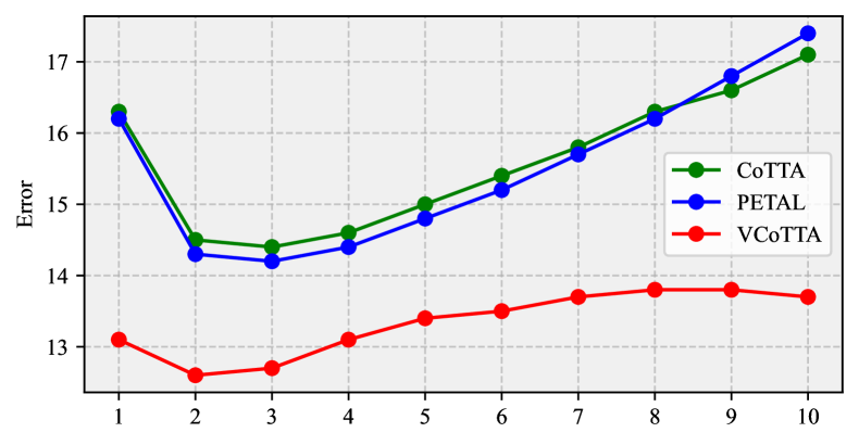
Figure 3: 10 loops under a same corruption order (CIFAR10C).

5.10 Hyperparameter analysis

In this subsection, we analyze the two major hyperparameters in VCoTTA, i.e., the margin $\epsilon$ in Eq. (13) and the number of augmentation in Eq. (10). We experimentally validate these hyperparameters with more choices. Experimental results are shown in Table 9 and Table 10. The results indicate that different datasets may require different margins as thresholds to control confidence. Additionally, increasing the number of augmentations can enhance effectiveness, but this hyperparameter ceases to have a significant impact after reaching 32.

Table 9: Analysis on confidence margin.

No.	$\epsilon$	CIFAR10C	$\epsilon$	CIFAR100C	$\epsilon$	ImageNetC
1	0	13.23	0	28.78	0	65.0
2	1e-4	13.23	0.1	28.55	1e-3	65.0
3	1e-3	13.22	0.2	28.45	1e-2	64.8
4	1e-2	13.14	0.3	28.43	1e-1	64.7
5	1e-1	13.31	0.4	28.54	2e-1	66.2

Table 10: Different number of augmentation.

Method	0	4	8	16	32	64
CoTTA	17.5	17.0	16.6	16.5	16.3	16.2
PETAL	17.3	16.9	16.4	16.1	16.0	16.0
VCoTTA	14.9	13.8	13.6	13.3	13.1	13.1

6 Conclusion

To tackle the prior drift problem, in this paper, we proposed a variational Bayesian inference approach, termed VCoTTA, to estimate uncertainties in CTTA. At the source stage, we first transformed an off-the-shelf pre-trained deterministic model into a Bayesian Neural Network (BNN) using a variational warm-up strategy, thereby injecting uncertainty into the source model. At the test time, we implemented a mean-teacher update strategy, where the student model is updated via variational inference, while the teacher model is refined by the exponential moving average. Specifically, to update the student model, we proposed a novel approach that utilizes a mixture of priors from both the source and teacher models. Consequently, the evidence lower bound can be formulated as the cross-entropy between the student and teacher models, combined with the Kullback-Leibler (KL) divergence of the prior mixture. We demonstrated the effectiveness of the proposed method on three datasets, and the results show that the proposed method can mitigate the issue of prior drift within the CTTA framework.

Appendix A CTTA approximation by Bayesian inference (BI)

The goal of CTTA is to learn a posterior distribution $p(\boldsymbol{\theta}|\mathcal{U}_{1:T}\cup\mathcal{D}_{0})$ from a source dataset $\mathcal{D}_{0}$, and a sequence of unlabeled test data from $\mathcal{U}_{1}$ to $\mathcal{U}_{T}$. Following Zhou & Levine (2021), assuming we have multiple input-generating distributions that the source dataset $\mathcal{D}_{0}$ is drawn from a distribution $\phi$, and $\tilde{\phi}_{t}$ specifies the shifted of the $t$-th unlabeled test dataset which we aim to adapt to. Let the parameters of the model be $\boldsymbol{\theta}$,then following the semi-supervised learning framework (Grandvalet & Bengio, 2004), we incorporate all input-generating distributions into the belief over the model parameters $\boldsymbol{\theta}$ as follows

$$p(\boldsymbol{\theta}|\phi,\tilde{\phi}_{1},\cdots,\tilde{\phi}_{T}) \propto p(\boldsymbol{\theta})\exp\left(-\lambda_{0}H_{\boldsymbol{\theta},\phi}(Y|\boldsymbol{X})\right)\prod_{t=1}^{T}\exp\left(-\lambda_{t}H_{\boldsymbol{\theta},\tilde{\phi}_{t}}(Y|\boldsymbol{X})\right),$$ (20)

where the inputs $X$ are sampled i.i.d. from a generative model with parameters $\phi$, while the corresponding labels $Y$ are sampled from a conditional distribution $p(Y|X,\boldsymbol{\theta})$, which is parameterized by the model parameters $\boldsymbol{\theta}$. $p(\boldsymbol{\theta})$ is a prior distribution over $\boldsymbol{\theta}$. $\{\lambda_{0},\lambda_{1},\cdots,\lambda_{T}\}$ are the factors for approximation weighting. Generally, the entropy term $H_{\boldsymbol{\theta},\phi}(Y|\boldsymbol{X})$ represents the cross entropy of the supervised learning, and the entropy term $H_{\boldsymbol{\theta},\tilde{\phi}_{t}}(Y|\boldsymbol{X})$ for $t>0$ denotes the Shannon entropy of the unsupervised learning.

Following Zhou & Levine (2021), we can empirically use a point estimation to get a plug-in Bayesian approach to approximate the above formula:

$$p(\boldsymbol{\theta}|\mathcal{U}_{1:T}\cup\mathcal{D}_{0})\propto p(\boldsymbol{\theta})\prod_{\forall x,y\in\mathcal{D}_{0}}p(y|x,\boldsymbol{\theta})\exp\left(-\frac{\lambda_{0}}{|\mathcal{D}_{0}|}\sum_{\forall x\in\mathcal{D}_{0}}{H}(Y|{x},\boldsymbol{\theta})\right)\prod_{t=1}^{T}\exp\left(-\frac{\lambda_{t}}{|\mathcal{U}_{t}|}\sum_{\forall x\in\mathcal{U}_{t}}{H}(Y|{x},\boldsymbol{\theta})\right).$$ (21)

To make the formula feasible to CTTA, that is, no source data is available at the test time, we set $\lambda_{0}=0$. And the source knowledge can be represented by $p(\boldsymbol{\theta}|\mathcal{D}_{0})\propto p(\boldsymbol{\theta})\prod_{\forall x,y\in\mathcal{D}_{0}}p(y|x,\boldsymbol{\theta})$. Thus, for the $t$-th test domain, the Bayesian inference in CTTA can be represented as follows:

$$p(\boldsymbol{\theta}|\mathcal{U}_{1:t}\cup\mathcal{D}_{0}) \propto p(\boldsymbol{\theta}|\mathcal{D}_{0})\prod_{i=1}^{t}\exp\left(-\frac{\lambda_{i}}{|\mathcal{U}_{i}|}\sum_{\forall x\in\mathcal{U}_{i}}{H}(Y|{x},\boldsymbol{\theta})\right)$$ (22)

$$\propto p(\boldsymbol{\theta}|\mathcal{U}_{1:t-1}\cup\mathcal{D}_{0})\exp\left(-\frac{\lambda_{t}}{|\mathcal{U}_{t}|}\sum_{\forall x\in\mathcal{U}_{t}}{H}(Y|{x},\boldsymbol{\theta})\right),$$

where $H(\mathcal{U}_{t}|\boldsymbol{\theta})=\cfrac{1}{|\mathcal{U}_{t}|}\sum_{\forall x\in\mathcal{U}_{t}}{H}(Y|{x},\boldsymbol{\theta})$ and the above formula can be rewritten in simplicity as

$$p(\boldsymbol{\theta}|\mathcal{U}_{1:t}\cup\mathcal{D}_{0})\propto p(\boldsymbol{\theta}|\mathcal{U}_{1:t-1}\cup\mathcal{D}_{0})e^{-\lambda H(\mathcal{U}_{t}|\boldsymbol{\theta})}=p_{t}(\boldsymbol{\theta})e^{-\lambda H(\mathcal{U}_{t}|\boldsymbol{\theta})},$$ (23)

which specifies the Bayesian inference process on continuously arriving unlabeled data in CTTA.

Appendix B ELBO of the VI in CTTA

We built VI for CTTA in Sec. 3, where we initialize a variational distribution $q(\boldsymbol{\theta})$ to approximate the real posterior. For the test domain $t$, we optimize the variational distribution as follows:

$$q_{t}(\boldsymbol{\theta})=\arg\min_{q\in\mathbb{Q}}\mathrm{KL}\left[q(\boldsymbol{\theta})\parallel\frac{1}{Z_{t}}p_{t}(\boldsymbol{\theta})e^{-{\lambda}{H}(\mathcal{U}_{t}|\boldsymbol{\theta})}\right],$$ (24)

where $\mathbb{Q}$ is the distribution searching space, and $p_{t}(\boldsymbol{\theta})$ is the current prior.

Following the definition of KL divergence and the standard derivation of the Evidence Lower BOund (ELBO) is as the following formulas. Specifically, the KL divergence is expanded as

$$\mathrm{KL}\left[q(\boldsymbol{\theta})\parallel\cfrac{1}{Z_{t}}p_{t}(\boldsymbol{\theta})e^{-\lambda H(\mathcal{U}_{t}|\boldsymbol{\theta})}\right] =-\int_{\boldsymbol{\theta}}q(\boldsymbol{\theta})\log\cfrac{\cfrac{1}{Z_{t}}p_{t}(\boldsymbol{\theta})e^{-\lambda H(\mathcal{U}_{t}|\boldsymbol{\theta})}}{q(\boldsymbol{\theta})}d\boldsymbol{\theta}$$ (25)

$$=-\int_{\boldsymbol{\theta}}q(\boldsymbol{\theta})\log\cfrac{1}{Z_{t}}e^{-\lambda H(\mathcal{U}_{t}|\boldsymbol{\theta})}d\boldsymbol{\theta}-\int_{\boldsymbol{\theta}}q(\boldsymbol{\theta})\log\cfrac{p_{t}(\boldsymbol{\theta})}{q(\boldsymbol{\theta})}d\boldsymbol{\theta}$$

$$=\int_{\boldsymbol{\theta}}q(\boldsymbol{\theta})\log Z_{t}d\boldsymbol{\theta}+\lambda\int_{\boldsymbol{\theta}}q(\boldsymbol{\theta})H(\mathcal{U}_{t}|\boldsymbol{\theta})d\boldsymbol{\theta}-\int_{\boldsymbol{\theta}}q(\boldsymbol{\theta})\log\cfrac{p_{t}(\boldsymbol{\theta})}{q(\boldsymbol{\theta})}d\boldsymbol{\theta}$$

$$=\log Z_{t}+\lambda\mathbb{E}_{\boldsymbol{\theta}\sim q(\boldsymbol{\theta})}H(\mathcal{U}_{t}|\boldsymbol{\theta})+\mathrm{KL}\left(q(\boldsymbol{\theta})\parallel p_{t}(\boldsymbol{\theta})\right),$$

where the first constant term can be reduced in the optimization. Thus, we can optimize the variational distribution via the ELBO:

$$q_{t}(\boldsymbol{\theta}) =\arg\min_{q\in\mathbb{Q}}\mathrm{KL}\left[q(\boldsymbol{\theta})\parallel\frac{1}{Z_{t}}p_{t}(\boldsymbol{\theta})e^{-{\lambda}{H}(\mathcal{U}_{t}|\boldsymbol{\theta})}\right]$$ (26)

$$=\arg\max_{q\in\mathbb{Q}}-\lambda\mathbb{E}_{\boldsymbol{\theta}\sim q(\boldsymbol{\theta})}H(\mathcal{U}_{t}|\boldsymbol{\theta})-\mathrm{KL}\left(q(\boldsymbol{\theta})\parallel p_{t}(\boldsymbol{\theta})\right)$$

$$=\arg\max_{q\in\mathbb{Q}}\text{ELBO}.$$

Optimization soving: In our case, the former entropy term can be more effectively replaced by the cross entropy or symmetric cross entropy (SCE) between the student model and the teacher model in a mean-teacher architecture (see Sec. 4.1). For the latter KL term, we can substitute a variational approximation that we deem closest to the current-stage prior $p_{t}(\boldsymbol{\theta})$ into the KL divergence. When the prior is a multivariate Gaussian distribution, this term can be computed in closed form as

$$\mathrm{KL}\left(\mathcal{N}(\boldsymbol{\mu}_{1},\boldsymbol{\Sigma}_{1})\parallel\mathcal{N}(\boldsymbol{\mu}_{2},\boldsymbol{\Sigma}_{2})\right)=\frac{1}{2}\left(\text{tr}(\boldsymbol{\Sigma}_{2}^{-1}\boldsymbol{\Sigma}_{1})+(\boldsymbol{\mu}_{2}-\boldsymbol{\mu}_{1})^{\top}\boldsymbol{\Sigma}_{2}^{-1}(\boldsymbol{\mu}_{2}-\boldsymbol{\mu}_{1})-k+\ln\left(\frac{\det(\boldsymbol{\Sigma}_{2})}{\det(\boldsymbol{\Sigma}_{1})}\right)\right).$$ (27)

where $\boldsymbol{\Sigma}=\text{diag}(\boldsymbol{\sigma^{2}})$, $k$ represents the dimensionality of the distributions, $\text{tr}(\cdot)$ denotes the trace of a matrix, and $\det(\cdot)$ stands for the determinant of a matrix. For the case that the prior is a mixture of Gaussian distributions, we can refer to the next section to get its upper bound.

Appendix C Mixture-of-Gaussian Prior

We refer to the lemma that was stated for the mixture of Gaussian in Singer & Warmuth (1998).

Lemma C.1.

The KL divergence between two mixture distributions $p=\sum_{i=1}^{k}\alpha_{i}p_{i}$ and $p^{\prime}=\sum_{i=1}^{k}\alpha_{i}p^{\prime}_{i}$ is upper-bounded by

$$\mathrm{KL}(p\parallel p^{\prime})\leq\mathrm{KL}(\boldsymbol{\alpha}\parallel\boldsymbol{\alpha}^{\prime})+\sum_{i=1}^{k}\alpha_{i}\mathrm{KL}(p_{i}\parallel p^{\prime}_{i}),$$ (28)

where $\boldsymbol{\alpha}=(\alpha_{1},\alpha_{2},\cdots,\alpha_{k})$ and $\boldsymbol{\alpha}^{\prime}=(\alpha^{\prime}_{1},\alpha^{\prime}_{2},\cdots,\alpha^{\prime}_{k})$ are the weights of the mixture components. The equality holds if and only if ${\alpha_{i}p_{i}}/{\sum_{j=1}^{k}\alpha_{j}p_{j}}={\alpha^{\prime}_{i}p^{\prime}_{i}}/{\sum_{j=1}^{k}\alpha^{\prime}_{j}p^{\prime}_{j}}$ for all $i$.

Proof.

Using the log-sum inequality (Cover, 1999), we have

$$\mathrm{KL}(\sum_{i=1}^{k}\alpha_{i}p_{i}\parallel\sum_{i=1}^{k}\alpha_{i}p^{\prime}_{i}) =\int\left(\sum_{i=1}^{k}\alpha_{i}p_{i}\right)\log\cfrac{\sum_{i=1}^{k}\alpha_{i}p_{i}}{\sum_{i=1}^{k}\alpha_{i}p^{\prime}_{i}}$$

$$\leq\int\sum_{i=1}^{k}\alpha_{i}p_{i}\log\cfrac{\alpha_{i}p_{i}}{\alpha_{i}p^{\prime}_{i}}$$

$$=\sum_{i=1}^{k}\alpha_{i}\left(\int p_{i}\log\cfrac{\alpha_{i}}{\alpha_{i}^{\prime}}+\int p_{i}\log\cfrac{p_{i}}{p^{\prime}_{i}}\right)$$

$$=\mathrm{KL}(\boldsymbol{\alpha}\parallel\boldsymbol{\alpha}^{\prime})+\sum_{i=1}^{k}\alpha_{i}\mathrm{KL}(p_{i}\parallel p^{\prime}_{i}).$$

∎

In our algorithm, $q(\boldsymbol{\theta})$ is set to be a mixture of Gaussian distributions, i.e., $p_{t}(\boldsymbol{\theta})=\alpha\cdot p_{1}(\boldsymbol{\theta})+(1-\alpha)\cdot\bar{p}_{t}(\boldsymbol{\theta})$. In the above inequality, let $q(\boldsymbol{\theta})=\sum_{i=1}^{k}\alpha_{i}q(\boldsymbol{\theta})$, we can get the upper bound of the KL divergence between $q(\boldsymbol{\theta})$ and $p_{t}(\boldsymbol{\theta})$:

$$\mathrm{KL}(q\parallel p_{t})\leq\alpha\cdot\text{KL}\left(q||{p}_{1}\right)+(1-\alpha)\cdot\text{KL}\left(q||\bar{p}_{t}\right).$$ (29)

So the lower bound (26) can be redefined as

$$\mathcal{L} =-\lambda\mathbb{E}_{\boldsymbol{\theta}\sim q(\boldsymbol{\theta})}H(\mathcal{U}_{t}|\boldsymbol{\theta})-\mathrm{KL}\left(q(\boldsymbol{\theta})\parallel p_{t}(\boldsymbol{\theta})\right)$$ (30)

$$\geq-\lambda\mathbb{E}_{\boldsymbol{\theta}\sim q(\boldsymbol{\theta})}H(\mathcal{U}_{t}|\boldsymbol{\theta})-\alpha\cdot\text{KL}\left(q||{p}_{1}\right)-(1-\alpha)\cdot\text{KL}\left(q||\bar{p}_{t}\right)\stackrel{{\scriptstyle\text{def}}}{{=}}\mathcal{L}^{\prime},$$

Then, we have obtained a lower bound that can be optimized through closed-form calculations as the source prior distribution $q_{0}(\boldsymbol{\theta})$ and the teacher prior distribution $\bar{q}_{t}(\boldsymbol{\theta})$ are multivariate Gaussian distributions, which means we can also optimize $\mathcal{L}^{\prime}$ with Eq. (27).

Appendix D Recursive variational approximation process in VCoTTA

In this section, we construct a complete algorithmic workflow utilizing variational approximation in VCoTTA.

Before test time: First, we adopt a variational warm-up strategy to inject stochastic dynamics into the model before adaptation. Given the source dataset $\mathcal{D}_{0}$, we can use a variational approximation of $p(\boldsymbol{\theta}|\mathcal{D}_{0})$ as follows

$$p(\boldsymbol{\theta}|\mathcal{D}_{0})=p_{1}(\boldsymbol{\theta})\approx q_{0}(\boldsymbol{\theta})=\arg\min_{q\in\mathbb{Q}}\mathrm{KL}\left[q(\boldsymbol{\theta})\parallel\frac{1}{Z_{0}}p(\boldsymbol{\theta})p(\mathcal{D}_{0}|\boldsymbol{\theta})\right],$$ (31)

where we use the pretrained deterministic model $p_{0}(\boldsymbol{\theta})$ as the prior distribution.

When the domain shift: Then, at the beginning of the test time, we set the prior in task $t$ as $p_{t}(\boldsymbol{\theta})=\alpha\cdot p_{1}(\boldsymbol{\theta})+(1-\alpha)\cdot\bar{p}_{t}(\boldsymbol{\theta})$ and variational approximation, where $p_{1}(\boldsymbol{\theta})\approx q_{0}(\boldsymbol{\theta})$ and $\bar{p}_{t}(\boldsymbol{\theta})\approx\bar{q}_{t}(\boldsymbol{\theta})$. For $\bar{q}_{t}(\boldsymbol{\theta})$, which means the real-time posterior probability of the teacher model for the $t$-th test domain, is constantly updated by $q_{t}(\boldsymbol{\theta})$ via EMA (see Sec. 4.3.3) during the test phase. Note that we do not have $\bar{q}_{t}(\boldsymbol{\theta})$ for the first update in the $t$-th phase. In fact, we use $q_{t-1}(\boldsymbol{\theta})$ construct the prior. In this scenario, we use $p_{t}(\boldsymbol{\theta})\approx\alpha\cdot p_{1}(\boldsymbol{\theta})+(1-\alpha)\cdot q_{t-1}(\boldsymbol{\theta})$. This is the variational distribution that should be used to approximate the prior in the absence of a teacher model in the first step, as well as the approximation that should be used when not employing the MT architecture. That is, using the posterior approximation from the previous domain to approximate the prior of the next domain is somehow like Nguyen et al. (2018). Note that the process is not required to inform the model that the domain produces a shift.

During a test domain: With the approximation to $p_{t}(\boldsymbol{\theta})$ and analysis from Appendix A, we can get $q_{t}(\boldsymbol{\theta})$ for student model at the test domain $t$ as follows:

$$q_{t}(\boldsymbol{\theta})=\arg\min_{q\in\mathbb{Q}}\mathrm{KL}\left[q(\boldsymbol{\theta})\parallel\frac{1}{Z_{t}}p_{t}(\boldsymbol{\theta})e^{-{\lambda}{H}(\mathcal{U}_{t}|\boldsymbol{\theta})}\right],$$ (32)

which means, we can recursively derive $p_{t+1}(\boldsymbol{\theta})$ and the following variational distributions, thereby achieving the goal of VCoTTA.

References

- Box & Tiao (2011) Box, G. E. and Tiao, G. C. Bayesian inference in statistical analysis. John Wiley & Sons, 2011.
- Brahma & Rai (2023) Brahma, D. and Rai, P. A probabilistic framework for lifelong test-time adaptation. In Proceedings of the Computer Vision and Pattern Recognition, 2023.
- Brier (1950) Brier, G. W. Verification of forecasts expressed in terms of probability. Journal of the Monthly Weather Review, 78(1):1–3, 1950.
- Bui et al. (2016) Bui, T., Hernández-Lobato, D., Hernandez-Lobato, J., Li, Y., and Turner, R. Deep gaussian processes for regression using approximate expectation propagation. In Proceedings of the International Conference on Machine Learning, 2016.
- Chakrabarty et al. (2023) Chakrabarty, G., Sreenivas, M., and Biswas, S. Sata: Source anchoring and target alignment network for continual test time adaptation. arXiv preprint arXiv:2304.10113, 2023.
- Chen et al. (2022) Chen, D., Wang, D., Darrell, T., and Ebrahimi, S. Contrastive test-time adaptation. In Proceedings of the Computer Vision and Pattern Recognition, 2022.
- Choi et al. (2022) Choi, S., Yang, S., Choi, S., and Yun, S. Improving test-time adaptation via shift-agnostic weight regularization and nearest source prototypes. In Procedings of the European Conference on Computer Vision, 2022.
- Cover (1999) Cover, T. M. Elements of information theory. John Wiley & Sons, 1999.
- Döbler et al. (2023) Döbler, M., Marsden, R. A., and Yang, B. Robust mean teacher for continual and gradual test-time adaptation. In Proceedings of the Computer Vision and Pattern Recognition, 2023.
- Du et al. (2023) Du, K., Lyu, F., Li, L., Hu, F., Feng, W., Xu, F., Xi, X., and Cheng, H. Multi-label continual learning using augmented graph convolutional network. IEEE Transactions on Multimedia, 2023.
- Ebrahimi et al. (2019) Ebrahimi, S., Elhoseiny, M., Darrell, T., and Rohrbach, M. Uncertainty-guided continual learning with bayesian neural networks. In Procedings of the International Conference on Learning Representations, 2019.
- Farquhar & Gal (2019) Farquhar, S. and Gal, Y. A unifying bayesian view of continual learning. arXiv preprint arXiv:1902.06494, 2019.
- Fortuin et al. (2021) Fortuin, V., Garriga-Alonso, A., Ober, S. W., Wenzel, F., Ratsch, G., Turner, R. E., van der Wilk, M., and Aitchison, L. Bayesian neural network priors revisited. In Procedings of the International Conference on Learning Representations, 2021.
- Friston et al. (2007) Friston, K., Mattout, J., Trujillo-Barreto, N., Ashburner, J., and Penny, W. Variational free energy and the laplace approximation. Journal of the Neuroimage, 34(1):220–234, 2007.
- Gal & Ghahramani (2016) Gal, Y. and Ghahramani, Z. Dropout as a bayesian approximation: Representing model uncertainty in deep learning. In Procedings of the International Conference on Machine Learning, 2016.
- Gandelsman et al. (2022) Gandelsman, Y., Sun, Y., Chen, X., and Efros, A. Test-time training with masked autoencoders. In Procedings of the Advances in Neural Information Processing Systems, 2022.
- Gelman et al. (1995) Gelman, A., Carlin, J. B., Stern, H. S., and Rubin, D. B. Bayesian data analysis. Chapman and Hall/CRC, 1995.
- Gneiting & Raftery (2007) Gneiting, T. and Raftery, A. E. Strictly proper scoring rules, prediction, and estimation. Journal of the American Statistical Association, 102(477):359–378, 2007.
- Grandvalet & Bengio (2004) Grandvalet, Y. and Bengio, Y. Semi-supervised learning by entropy minimization. In Proceedings of the Advances in Neural Information Processing Systems, 2004.
- He et al. (2016) He, K., Zhang, X., Ren, S., and Sun, J. Deep residual learning for image recognition. In Proceedings of the Computer Vision and Pattern Recognition, 2016.
- Hernández-Lobato & Adams (2015) Hernández-Lobato, J. M. and Adams, R. Probabilistic backpropagation for scalable learning of bayesian neural networks. In Procedings of the International Conference on Machine Learning, 2015.
- Huang et al. (2022) Huang, H., Gu, X., Wang, H., Xiao, C., Liu, H., and Wang, Y. Extrapolative continuous-time bayesian neural network for fast training-free test-time adaptation. In Proceedings of the Advances in Neural Information Processing Systems, 2022.
- Hunter (1986) Hunter, J. S. The exponentially weighted moving average. Journal of the Quality Technology, 18(4):203–210, 1986.
- Jain & Learned-Miller (2011) Jain, V. and Learned-Miller, E. Online domain adaptation of a pre-trained cascade of classifiers. In Proceedings of the Computer Vision and Pattern Recognition, 2011.
- Kingma et al. (2015) Kingma, D. P., Salimans, T., and Welling, M. Variational dropout and the local reparameterization trick. In Proceedings of the Advances in Neural Information Processing Systems, 2015.
- Kurle et al. (2019) Kurle, R., Cseke, B., Klushyn, A., Van Der Smagt, P., and Günnemann, S. Continual learning with bayesian neural networks for non-stationary data. In Procedings of the International Conference on Learning Representations, 2019.
- Li & Hoiem (2017) Li, Z. and Hoiem, D. Learning without forgetting. Journal of the IEEE Transactions on Pattern Analysis and Machine Intelligence, 40(12):2935–2947, 2017.
- (28) Liu, D., Lyu, F., Li, L., Xia, Z., and Hu, F. Centroid distance distillation for effective rehearsal in continual learning. In Proceedings of the IEEE International Conference on Acoustics, Speech and Signal Processing. IEEE.
- Liu et al. (2019) Liu, G., Liu, Y., Guo, M., Li, P., and Li, M. Variational inference with gaussian mixture model and householder flow. Journal of the Neural Networks, 109:43–55, 2019.
- Liu et al. (2021) Liu, Y., Kothari, P., Van Delft, B., Bellot-Gurlet, B., Mordan, T., and Alahi, A. Ttt++: When does self-supervised test-time training fail or thrive? In Procedings of the Advances in Neural Information Processing Systems, 2021.
- Louizos & Welling (2017) Louizos, C. and Welling, M. Multiplicative normalizing flows for variational bayesian neural networks. In Procedings of the International Conference on Machine Learning, 2017.
- Lyu et al. (2021) Lyu, F., Wang, S., Feng, W., Ye, Z., Hu, F., and Wang, S. Multi-domain multi-task rehearsal for lifelong learning. In Proceedings of the AAAI Conference on Artificial Intelligence, 2021.
- Lyu et al. (2023) Lyu, F., Sun, Q., Shang, F., Wan, L., and Feng, W. Measuring asymmetric gradient discrepancy in parallel continual learning. In Proceedings of the IEEE/CVF International Conference on Computer Vision, 2023.
- Mummadi et al. (2021) Mummadi, C. K., Hutmacher, R., Rambach, K., Levinkov, E., Brox, T., and Metzen, J. H. Test-time adaptation to distribution shift by confidence maximization and input transformation. arXiv preprint arXiv:2106.14999, 2021.
- Nguyen et al. (2018) Nguyen, C. V., Li, Y., Bui, T. D., and Turner, R. E. Variational continual learning. In Proceedings of the International Conference on Learning Representations, 2018.
- Ovadia et al. (2019) Ovadia, Y., Fertig, E., Ren, J., Nado, Z., Sculley, D., Nowozin, S., Dillon, J., Lakshminarayanan, B., and Snoek, J. Can you trust your model’s uncertainty? evaluating predictive uncertainty under dataset shift. In Proceedings of the Advances in Neural Information Processing Systems, 2019.
- Ritter et al. (2018) Ritter, H., Botev, A., and Barber, D. A scalable laplace approximation for neural networks. In Procedings of the International Conference on Learning Representations, 2018.
- Sato (2001) Sato, M.-A. Online model selection based on the variational bayes. Journal of the Neural Computation, 13:1649–1681, 2001.
- Schneider et al. (2020) Schneider, S., Rusak, E., Eck, L., Bringmann, O., Brendel, W., and Bethge, M. Improving robustness against common corruptions by covariate shift adaptation. In Proceedings of the Advances in Neural Information Processing Systems, 2020.
- Singer & Warmuth (1998) Singer, Y. and Warmuth, M. K. Batch and on-line parameter estimation of gaussian mixtures based on the joint entropy. In Procedings of the Advances in Neural Information Processing Systems, 1998.
- Sun et al. (2022) Sun, Q., Lyu, F., Shang, F., Feng, W., and Wan, L. Exploring example influence in continual learning. Proceedings of the Advances in Neural Information Processing Systems, 2022.
- Sun et al. (2020) Sun, Y., Wang, X., Liu, Z., Miller, J., Efros, A., and Hardt, M. Test-time training with self-supervision for generalization under distribution shifts. In Procedings of the International Conference on Machine Learning, 2020.
- Tarvainen & Valpola (2017) Tarvainen, A. and Valpola, H. Mean teachers are better role models: Weight-averaged consistency targets improve semi-supervised deep learning results. In Proceedings of the Advances in Neural Information Processing Systems, 2017.
- Wang et al. (2011) Wang, C., Paisley, J., and Blei, D. M. Online variational inference for the hierarchical dirichlet process. In Proceedings of the International Conference on Artificial Intelligence and Statistics, 2011.
- Wang et al. (2020) Wang, D., Shelhamer, E., Liu, S., Olshausen, B., and Darrell, T. Tent: Fully test-time adaptation by entropy minimization. In Proceedings of the International Conference on Learning Representations, 2020.
- Wang et al. (2022) Wang, Q., Fink, O., Van Gool, L., and Dai, D. Continual test-time domain adaptation. In Proceedings of the Computer Vision and Pattern Recognition, 2022.
- Wang et al. (2019) Wang, Y., Ma, X., Chen, Z., Luo, Y., Yi, J., and Bailey, J. Symmetric cross entropy for robust learning with noisy labels. In Proceedings of the Computer Vision and Pattern Recognition, 2019.
- Xie et al. (2017) Xie, S., Girshick, R., Dollár, P., Tu, Z., and He, K. Aggregated residual transformations for deep neural networks. In Proceedings of the Computer Vision and Pattern Recognition, 2017.
- Yang et al. (2023) Yang, X., Gu, Y., Wei, K., and Deng, C. Exploring safety supervision for continual test-time domain adaptation. In Proceedings of the International Joint Conference on Artificial Intelligence, 2023.
- Zagoruyko & Komodakis (2016) Zagoruyko, S. and Komodakis, N. Wide residual networks. In Procedings of the British Machine Vision Conference, 2016.
- Zhang et al. (2022) Zhang, M., Levine, S., and Finn, C. Memo: Test time robustness via adaptation and augmentation. In Procedings of the Advances in Neural Information Processing Systems, 2022.
- Zhao et al. (2022) Zhao, T., Wang, Z., Masoomi, A., and Dy, J. Deep bayesian unsupervised lifelong learning. Journal of the Neural Networks, 149:95–106, 2022.
- Zhou & Levine (2021) Zhou, A. and Levine, S. Bayesian adaptation for covariate shift. In Proceedings of the Advances in Neural Information Processing Systems, 2021.