A Projection-Based Time-Segmented Reduced Order Model for Fluid-Structure Interactions

Abstract

In this paper, a type of novel projection-based, time-segmented reduced order model (ROM) is proposed for dynamic fluid-structure interaction (FSI) problems based upon the arbitrary Lagrangian–Eulerian (ALE)-finite element method (FEM) in a monolithic frame, where spatially, each variable is separated from others in terms of their attribution (fluid/structure), category (velocity/pressure) and component (horizontal/vertical) while temporally, the proper orthogonal decomposition (POD) bases are constructed in some deliberately partitioned time segments tailored through extensive numerical trials. By the combination of spatial and temporal decompositions, the developed ROM approach enables prolonged simulations under prescribed accuracy thresholds. Numerical experiments are carried out to compare numerical performances of the proposed ROM with corresponding full-order model (FOM) by solving a two-dimensional FSI benchmark problem that involves a vibrating elastic beam in the fluid, where the performance of offline ROM on perturbed physical parameters in the online phase is investigated as well. Extensive numerical results demonstrate that the proposed ROM has a comparable accuracy to while much higher efficiency than the FOM. The developed ROM approach is dimension-independent and can be seamlessly extended to solve high dimensional FSI problems.

Keywords: Reduced order model (ROM); proper orthogonal decomposition (POD); full-order model (FOM); fluid-structure interaction (FSI); arbitrary Lagrangian–Eulerian (ALE) mapping; mixed finite element method (FEM)

1 Introduction

Fluid-structure interaction (FSI) phenomena are encountered in many engineering systems and biological processes, such as the vibration of turbine blades impacted by the fluid flow, the response of bridges and tall buildings to winds, the floating parachute wafted by the air current, the rotating mechanical parts driven by the pressurized liquid, the blood fluid through the cardiovascular system, and etc. Simulating FSI problems enables analyzing relevant engineering/biological system performance and durability under complex operating conditions and with an accurate fashion by monolithically considering the interactional effects between the fluid and structure through subtle interface conditions (which have two kinds: the dynamic one and the kinematic one). However, high-fidelity FSI modeling presents immense computational challenges due to the need for interfacing distinct fluid and structural solvers. FSI simulations must couple solutions of the unsteady Navier-Stokes equations in the fluid domain, which is usually defined in Eulerian description, with solutions of potentially nonlinear structural dynamics in the Lagrangian-based structural domain. This requires exchanging the interface information at each time step while accounting for the moving interface thus moving subdomains and even moving meshes if a body-fitted mesh method is adopted.

When addressing numerical methods for solving FSI problems, two different categories always exist, as demonstrated below:

1. The body-fitted/unfitted mesh method in terms of the mesh conformity between the fluidic and structural meshes.

   The most representative body-fitted mesh method is the arbitrary Lagrangian–Eulerian (ALE) method (see e.g., [19, 17, 28, 39]) which adapts the fluid mesh to accommodate the deformations/displacements of structure on the interface, thus interface conditions are naturally satisfied therein. On the other hand, the fictitious domain/immersed boundary method (FD/IBM) (see e.g., [32, 33, 25, 27])represents the body-unfitted mesh method the most, where the fluid is extended into the structural domain as the fictitious fluid thus a fixed background Eulerian fluidic mesh fills up the entire domain, while the foreground Lagrangian structural mesh changes with time and thus does not conform with the fluidic mesh, simultaneously, the kinematic interface condition is also reinforced throughout the structural domain besides the interface, either strongly or weakly.

2. The monolithic/partitioned approach in terms of the coupling strategy between the fluid and structural solver.

   With the monolithic approach [45, 37, 24, 5], the fluid and structural equations are solved simultaneously, where the dynamic interface condition naturally vanishes in the variational/weak form of FSI while the kinematic interface condition is reinforced on the interface. It owns unconditional stability and the immunity of any systematic error in the implementation of interface conditions for moving interface (e.g., FSI) problems without doing an alternating iteration by subdomains. Whereas, the partitioned approach [13, 9, 38, 16] solves the fluid and structure equations, separately, by a Dirichlet/Robin-Neumann alternating iteration between the fluid and structural solver, where the kinematic interface condition is taken as Dirichlet boundary condition of fluid equations and the dynamic interface condition as Neumann boundary condition of structural equations. It is conditionally stable and conditionally convergent under a particular range of the physical parameters of FSI model. For instance, it fails to converge when fluid and structural densities are of the same magnitude due to the so-called added-mass effect [20, 9].

In regard to the above numerical methodologies, the full-order model (FOM) approach that we adopt to numerically solve FSI problems in this paper is the ALE-finite element method (ALE-FEM) within the monolithic frame, as the author Sun et al. do in [47, 14, 23, 22]. The FOM approach may undergo a large-scale computation over a long term evolvement, leading to a time-consuming FSI simulation with high computational costs in practice. As a contrast, the reduced-order model (ROM) approach [46, 26, 21, 3, 4, 30], which constructs low-dimensional surrogate models by projecting governing equations onto a compact modal basis, can provide a computationally inexpensive possibility to perform the same computations as the FOM does but with minimum complexity while keeping the essential features of the system intact. Thus the ROM may radically accelerate detailed FSI simulations and save a great deal of computational costs while remain a comparable accuracy to the FOM.

Traditionally, utilizing the ROM to solve fluid dynamics is to apply the Galerkin projection to Navier-Stokes equations within the space spanned by the time-invariant, proper orthogonal decomposition (POD) bases, which induces reduced ODE systems with respect to spatial variables, and then the spatial integration is performed to obtain space-invariant POD coefficients [34]. As for FSI problems, ROM is studied with either the partitioned or monolithic approach. For instance, in the partitioned approach, two distinct ROMs are normally adopted to solve fluid and structural equations in their respective domains first, and then are coupled together to form a ROM for FSI [6, 44, 21, 34]. Additionally, the moving interface of fluid and structure can also be brought into the formation of ROM for FSI [44]. When the ALE-based body-fitted mesh method is applied, the fluidic mesh moves along with structural deformations, which sways over POD modes and thus induces a multi-POD approach in [1] by selecting bases on grid shifts. The aforementioned Galerkin POD-ROM approach is also proposed to account for modest deformation cases when capturing the transonic flow’s capricious nature [8] and when solving generic FSI problems [31], which shows that in the online phase of ROM, the dimension of online FSI system can still be reduced further with minor modifications like variable changes and careful selections of interface coupling. ROM-ROM and ROM-FOM coupling strategies are also actively developed for interface problems in the field of model order reduction [15, 11, 7], and the current research into coupled ROM systems promises additional performance gains [2], showing that the ROM is an extremely interesting approach that could benefit many FSI-related applications.

Because FSI problems are parameter-dependent problems, an extra assumption, i.e., all operators in FSI problems hold an affine parametric dependence, needs to be made in order to enable fast online parametric queries. The empirical interpolation method can recover this affine dependence, but with many parametrized functions, which adds major offline costs. This tradeoff is necessary to decouple expensive, one-time, parameter-independent high-fidelity data structures from inexpensive, parameter-dependent online queries. For instance, domains of varying shapes are considered in [36] that are parametrized by affine and non-affine maps related to a reference domain, where the proposed method is well-suited for repeated and rapid evaluations needed for parameter estimation, design, optimization, and real-time control. In [10], a projection-based ROM using POD and discrete empirical interpolation method, together with a characteristic-based split scheme, is applied to the ALE-based Navier-Stokes equations on dynamic grids. A monolithic approach of ROM for parametrized FSI problems is put forth in [3], where a detailed parametrized formulation of FSI and its components is provided to demonstrate how an efficient offline-online computation by approximating parametrized nonlinear tensors is achieved. In addition, the monolithic POD-Galerkin method is also presented therein to show how the fluid velocity, pressure and structural displacement of FSI problems are efficiently computed during the online phase.

In this paper, we intend to develop a monolithic ALE-FEM based, novel POD-ROM to solve dynamic FSI problems undergoing a long-term evolvement. It is well known that the traditional POD-ROM approach may blow up for extended simulations after a long run, as revealed by e.g., [40] or the authors Zhai et al. [48] in which the comparison error between ROM and FOM for parabolic equations under fixed POD bases increases with time, and the error can only be controlled within $O(\tau^{-\frac{1}{2}})$ time steps, where $\tau$ is the time step size. This inspires us to first consider a construction of unsteady POD bases that vary in each time segment, where all time segments are divided from the entire time interval as a coarse partition, then to conduct the online POD-ROM computation following these time segments. Our numerical results in Section 4.2 also show that if the time dimension is not segmented and the POD bases are independent of time, then the total relative $L^{2}$ error between ROM and FOM reaches up to the magnitude of $10^{11}$, causing an error blowup for the ROM to FSI simulation. To the best of our knowledge, so far there has not such a time-segmented idea being proposed for ROM yet on solutions to time-dependent problems including FSI.

Based upon the above insights, our commitments in this paper are as follows:

• In an innovative fashion, treat time as a non-reduced variable and design a new ROM approach by dividing the entire time interval into some typical time segments, then carrying out the classical POD method following these time segments.

• Apply the developed ROM to a FSI benchmark problem involving a vibrating elastic beam in the fluid, and suppress the increasing error of the beam vibration’s amplitude at the tail part after a long-term simulation.

• Numerically demonstrate that the developed ROM not only remains a comparable accuracy to the FOM but also adapts to perturbed model parameters.

The structure of this paper is organized as follows. In Section 2, we introduce the generic FSI model and its fully discrete ALE-FEM. The ROM approach in both offline and online phases are proposed in Section 3. We conduct numerical experiments in Section 4 to validate the proposed ROM by comparing with FOM on solutions to a FSI benchmark problem. Finally, the concluding remarks are given in Section 5.

2 Model description and finite element method for FSI

Let $\Omega\subset\mathbb{R}^{d}\ (d=2,3)$ be an open bounded domain of interest with a polygonal boundary $\partial\Omega$, which is divided by the interface $\Gamma_{FSI}(t)$ into two subdomains: $\Omega=\Omega_{f}(t)\cup\Omega_{s}(t)$ and $\Gamma_{FSI}(t)=\bar{\Omega}_{f}(t)\cap\bar{\Omega}_{s}(t)\ (t\in[0,T])$, where $\Omega_{f}(t)$ is the fluid domain and $\Omega_{s}(t)$ the structural domain, and $\Omega_{f}(t)\cap\Omega_{s}(t)=\varnothing$. Figure 1 illustrates a domain of a FSI benchmark problem [42, 43], where $\partial\Omega=\Gamma_{in}\cup\Gamma_{walls}\cup\Gamma_{out}$, $\Gamma_{in}$, $\Gamma_{walls}$ and $\Gamma_{out}$ represent the inlet, walls and outlet of the fluidic channel, respectively.

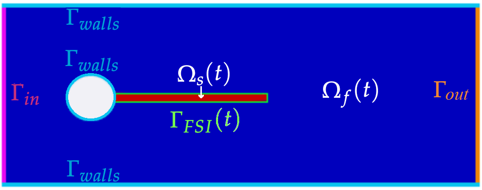
Figure 1: A schematic domain of FSI benchmark problem, where the fluid channel $\Omega_{f}(t)$ is in blue, the red-colored structural domain $\Omega_{s}(t)$ represents a elastic beam behind a rigid cylinder. From the left to right, lines in purple, cyan, green and orange represent the inlet $\Gamma_{in}$, the fluidic channel wall $\Gamma_{walls}$, the fluid-structure interface $\Gamma_{FSI}(t)$, and the outlet $\Gamma_{out}$, respectively.

2.1 Model of dynamic FSI problems

In the coupled multiphysics system of FSI, the fluid is assumed to be Newtonian and incompressible, therefore, its behavior can be modeled by incompressible Navier-Stokes equations in terms of the fluid velocity $\bm{u}_{f}$ and fluid pressure $p_{f}$: find $(\bm{u}_{f},p_{f})\in H^{1}(0,T;H^{2}(\Omega_{f}(t))^{d})\times L^{2}(0,T;H^{1}(\Omega_{f}(t)))$ such that

$$\left\{\begin{array}[]{rcll}\rho_{f}\left(\frac{\partial\bm{u}_{f}}{\partial t}+\left(\bm{u}_{f}\cdot\nabla\right)\bm{u}_{f}\right)-\operatorname{div}\bm{\sigma}_{f}\left(\bm{u}_{f},p_{f}\right)&=&\bm{b}_{f},&\text{in }\Omega_{f}(t)\times(0,T],\\ \operatorname{div}\bm{u}_{f}&=&0,&\text{in }\Omega_{f}(t)\times(0,T],\end{array}\right.$$ (1)

subjecting to the following boundary conditions and initial condition:

$$\begin{array}[]{rclll}\bm{u}_{f}&=&\bm{u}_{in},&\text{on }\Gamma_{in},&(\text{incoming flow condition})\\ \bm{u}_{f}&=&\bm{0},&\text{on }\Gamma_{walls},&(\text{no-slip condition})\\ \bm{\sigma}_{f}\bm{n}_{f}&=&\bm{0},&\text{on }\Gamma_{out},&(\text{do-nothing condition})\\ \bm{u}_{f}(\bm{x},0)&=&\bm{u}_{f}^{0},&\text{in }\hat{\Omega}_{f},&(\text{initial condition})\end{array}$$ (2)

where $\rho_{f}$ is the fluid density, $\bm{b}_{f}$ the fluid volume external force, $\bm{n}_{f}$ the outward normal unit vector on $\Gamma_{out}$, and $\bm{\sigma}_{f}\left(\bm{u}_{f},p_{f}\right)$ the fluid stress tensor that is expressed as follows:

$$\bm{\sigma}_{f}\left(\bm{u}_{f},p_{f}\right)=\rho_{f}\nu_{f}\left(\nabla\bm{u}_{f}+(\nabla\bm{u}_{f})^{T}\right)-p_{f}\bm{I},$$

here $\nu_{f}$ is the fluid kinematic viscosity, and $\bm{I}$ the identity matrix.

We note that the gradient operator “$\nabla$” and divergence operator “$\operatorname{div}$” in (1) and in what follows refer to differentiations with respect to the time-dependent spatial coordinates, $\bm{x}_{f}=\hat{\bm{X}}_{f}(\hat{\bm{x}}_{f},t)$, where $\bm{x}_{f}$ denotes the current/Eulerian coordinates in $\Omega_{f}(t)$ while $\hat{\bm{x}}_{f}$ denotes the initial/reference/Lagrangian coordinates in $\hat{\Omega}_{i}=\Omega_{i}(0)$, $i=f$ or $s$. In fact, $\bm{x}_{i}=\hat{\bm{X}}_{i}(\hat{\bm{x}}_{i},t)=\hat{\bm{x}}_{i}+\hat{\bm{d}}_{i}$ defines a bijective flow map, $\hat{\bm{X}}_{i}:\hat{\Omega}_{i}\mapsto\Omega_{i}(t)$, where $\hat{\bm{d}}_{i}$ denotes the material displacement in $\hat{\Omega}_{i}\ (i=f,s)$. Without further indication, we use “ $\hat{\cdot}$ ” to denote an object “ $\cdot$ ” that is associated with the initial/reference domain of $\Omega_{i}(t)$, $\hat{\Omega}_{i}\ (i=f,s)$, in the rest of this paper.

As for the structural material, we adopt the linear elasticity to model the structural constitution relation in this paper, which can be generalized to more complicated nonlinear structural materials. The structural dynamics can be defined below in terms of the structural displacement $\hat{\bm{d}}_{s}$: find $\hat{\bm{d}}_{s}(t)\in H^{2}(0,T;H^{2}(\hat{\Omega}_{s})^{d})$ such that:

$$\hat{\rho}_{s}\frac{\partial^{2}\hat{\bm{d}}_{s}}{\partial t^{2}}-\widehat{\operatorname{div}}\hat{\bm{P}}\left(\hat{\bm{d}}_{s}\right)=\hat{\bm{b}}_{s},\quad\text{ in }\hat{\Omega}_{s}\times(0,T],$$ (3)

where $\hat{\rho}_{s}$ is the structural density, $\hat{\bm{b}}_{s}$ is the external force acting on the structure, and $\hat{\bm{P}}\left(\hat{\bm{d}}_{s}\right)$ is the first Piola-Kirchhoff stress tensor expressed as

$$\hat{\bm{P}}\left(\hat{\bm{d}}_{s}\right)=2\mu_{s}\hat{\bm{\varepsilon}}\left(\hat{\bm{d}}_{s}\right)+\lambda_{s}\operatorname{tr}\hat{\bm{\varepsilon}}\left(\hat{\bm{d}}_{s}\right)\bm{I},$$

where $\mu_{s}$ and $\lambda_{s}$ denote the Lamé constants, and $\hat{\bm{\varepsilon}}\left(\hat{\bm{d}}_{s}\right)$ is the linearized strain operator defined as

$$\hat{\bm{\varepsilon}}\left(\hat{\bm{d}}_{s}\right):=\frac{1}{2}\left(\hat{\nabla}\hat{\bm{d}}_{s}+(\hat{\nabla}\hat{\bm{d}}_{s})^{T}\right).$$

Here the gradient operator “$\hat{\nabla}$” and divergence operator “$\widehat{\operatorname{div}}$” represent differentiations with respect to Lagrangian coordinates, $\hat{\bm{x}}_{s}$, in the reference configuration.

The following boundary condition and initial condition are defined for (3):

$$\begin{array}[]{rclll}\hat{\bm{d}}_{s}&=&0,&\text{on }\hat{\Gamma}_{walls}\cap\hat{\Gamma}_{FSI},&\text{(fixed support condition)}\\ \hat{\bm{d}}_{s}(\hat{\bm{x}},0)&=&\hat{\bm{d}}_{s}^{0},&\text{in }\hat{\Omega}_{s}.&\text{(initial condition)}\end{array}$$ (4)

To close the definition of FSI model, we need to introduce the following no-slip type interface conditions that can be applied to most cases of FSI problems,

$$\begin{array}[]{rclll}\bm{u}_{f}(\bm{x}(\hat{\bm{x}},t),t)&=&\frac{\partial\hat{\bm{d}}_{s}}{\partial t},&\text{on }\hat{\Gamma}_{FSI}\times[0,T],&\text{(kinematic condition)}\\ \hat{J}\bm{\sigma}_{f}(\bm{x}(\hat{\bm{x}},t),t)\hat{\bm{F}}^{-T}\hat{\bm{n}}_{s}&=&\hat{\bm{P}}\hat{\bm{n}}_{s},&\text{on }\hat{\Gamma}_{FSI}\times[0,T],&\text{(dynamic condition)}\end{array}$$ (5)

which describe the continuity of velocity and of normal stress across the interface, respectively, where the Jacobian matrix, $\hat{\bm{F}}=\hat{\nabla}_{\hat{\bm{x}}_{s}}\bm{x}_{s}=\hat{\nabla}_{\hat{\bm{x}}_{s}}\hat{\bm{X}}_{s}=\bm{I}+\hat{\nabla}_{\hat{\bm{x}}_{s}}\hat{\bm{d}}_{s}$, denotes the deformation gradient tensor of structure, $\hat{J}=\operatorname{det}(\hat{\bm{F}})$ is the Jacobian, and $\hat{\bm{n}}_{s}$ denotes the outward normal unit vector on $\hat{\Gamma}_{FSI}$ pointing into the fluid domain from the structural domain.

2.2 ALE mapping

Instead of using the material/Lagrangian mapping of fluid, $\hat{\bm{X}}_{f}$, to move the fluidic mesh that may suffer grid distortions due to the large displacement of fluidic material point, we introduce the following invertible ALE mapping:

$$\mathcal{\hat{\bm{A}}}_{f}:\hat{\Omega}_{f} \mapsto\Omega_{f}(t)$$

$$\hat{\bm{x}}_{f} \mapsto\bm{x}_{m}=\hat{\bm{x}}_{f}+\hat{\bm{m}}_{f},$$

where $\bm{x}_{m}\in\Omega_{f}(t)$ denotes the current position of fluidic mesh, $\hat{\bm{m}}_{f}$ denotes the fluidic mesh displacement that is defined as an extension of the structural displacement $\hat{\bm{d}}_{s}$ into $\hat{\Omega}_{f}$. This extension can be defined in different ways. Here we adopt a harmonic extension to define the ALE mapping:

$$\left\{\begin{array}[]{rcll}-\operatorname{div}\left(\hat{\nabla}\hat{\bm{m}}_{f}\right)&=&0,&\text{ in }\hat{\Omega}_{f},\\ \hat{\bm{m}}_{f}&=&\hat{\bm{d}}_{s},&\text{ on }\hat{\Gamma}_{FSI},\\ \hat{\bm{m}}_{f}&=&0,&\text{ on }\partial\hat{\Omega}_{f}\backslash\hat{\Gamma}_{FSI}.\end{array}\right.$$ (6)

Thus, the moving fluidic mesh is obtained by $\bm{x}_{m}=\hat{\bm{x}}_{f}+\hat{\bm{m}}_{f}$, $\forall\hat{\bm{x}}_{f}\in\hat{\Omega}_{f}$. Let ${\bm{v}}_{m}$ denote the velocity of fluidic mesh, defined as

$${\bm{v}}_{m}({\bm{x}_{m}},t)=\frac{\partial\mathcal{\hat{\bm{A}}}_{f}}{\partial t}\circ\mathcal{{\hat{\bm{A}}}}_{f}^{-1}({\bm{x}_{m}})=\frac{\partial(\hat{\bm{x}}_{f}+\hat{\bm{m}}_{f})}{\partial t}=\frac{\partial\hat{\bm{m}}_{f}}{\partial t}(\hat{\bm{x}}_{f},t).$$ (7)

Then we have the material derivative defined on the moving fluidic mesh as follows

$$D_{t}{\bm{u}}_{f}=\partial_{t}^{\mathcal{\hat{\bm{A}}}_{f}}{\bm{u}}_{f}+\big{(}({\bm{u}}_{f}-{\bm{v}}_{m})\cdot\nabla\big{)}{\bm{u}}_{f},$$ (8)

where $\partial_{t}^{\mathcal{\hat{\bm{A}}}_{f}}{\bm{u}}_{f}=\frac{\partial{\bm{u}}_{f}}{\partial t}+({\bm{v}}_{m}\cdot\nabla){\bm{u}}_{f}$ denotes the ALE material derivative. Hence, fluid equations (1) can be reformulated as follows in ALE description:

$$\left\{\begin{aligned} \rho_{f}\big{(}\partial_{t}^{\mathcal{\hat{\bm{A}}}_{f}}{\bm{u}}_{f}+(({\bm{u}}_{f}-{\bm{v}}_{m})\cdot\nabla){\bm{u}}_{f}\big{)}-\operatorname{div}{\bm{\sigma}}_{f}&={\bm{b}}_{f},&\hbox{~{}~{}~{}in~{}}\Omega_{f}(t)\times(0,T],\\ \operatorname{div}{\bm{u}}_{f}&=0,&\hbox{~{}in~{}}\Omega_{f}(t)\times(0,T].\end{aligned}\right.$$ (9)

The following Lemma 2.1 shows that the ALE mapping, $\mathcal{\hat{\bm{A}}}_{f}$, holds $H^{1}$-invariance all the time for any $\bm{u}_{f}(\bm{x}(\hat{\bm{x}},t),t)$ and its ALE material derivative $\partial_{t}^{\mathcal{\hat{\bm{A}}}_{f}}{\bm{u}}_{f}$.

Lemma 2.1

[12, 29] For any $t\in(0,T]$, $\bm{u}_{f}(\bm{x},t)\in H^{1}(\Omega_{f}(t))^{d}$ and $\partial_{t}^{\mathcal{\hat{\bm{A}}}_{f}}{\bm{u}}_{f}(\bm{x},t)\in H^{1}(\Omega_{f}(t))^{d}$ if and only if $\hat{\bm{u}}(\hat{\bm{x}},t)=\bm{u}(\bm{x},t)\circ\mathcal{\hat{\bm{A}}}_{f}(\hat{\bm{x}},t)\in H^{1}(\hat{\Omega}_{f})^{d}$.

2.3 Monolithic ALE-FEM for FSI

In this section, we depict the monolithic, fully discrete ALE-FEM for the presented FSI model (9), (2)-(6) as the author Sun et al. do in, e.g., [14, 47]. We first introduce the following Sobolev spaces that are adopted to define the ALE weak form of FSI model:

$$\begin{array}[]{rcl}\bm{V}^{f}&:=&\{\bm{\psi}_{f}\in H^{1}(\Omega_{f}(t))^{d}:\bm{\psi}_{f}=\hat{\bm{\psi}}_{f}\circ\mathcal{\hat{\bm{A}}}_{f}^{-1},\hat{\bm{\psi}}_{f}\in H^{1}(\hat{\Omega}_{f})^{d}\},\\ \vspace{0.2cm}\bm{V}^{f}_{0}&:=&\{\bm{\psi}_{f}\in\bm{V}^{f}:\bm{\psi}_{f}=\bm{0}\text{ on }\Gamma_{in}\cup\Gamma_{walls}\},\\ \vspace{0.2cm}\bm{V}^{f}_{D}&:=&\{\bm{\psi}_{f}\in\bm{V}^{f}:\bm{\psi}_{f}=\bm{u}_{in}\text{ on }\Gamma_{in},\bm{\psi}_{f}=\bm{0}\text{ on }\Gamma_{walls}\},\\ \vspace{0.2cm}\hat{\bm{V}}^{s}&:=&\{\hat{\bm{\psi}}_{s}\in H^{1}(\hat{\Omega}_{s})^{d}:\frac{\partial\hat{\bm{\psi}}_{s}}{\partial t}=\bm{\psi}_{f}\circ\mathcal{\bm{A}}_{f}\text{ on }\hat{\Gamma}_{FSI},\bm{\psi}_{f}\in\bm{V}^{f}\cap L^{2}(\Gamma_{FSI})\},\\ \vspace{0.2cm}\hat{\bm{V}}^{s}_{0}&:=&\{\hat{\bm{\psi}}_{s}\in\hat{\bm{V}}^{s}:\hat{\bm{\psi}}_{s}=\bm{0}\text{ on }\hat{\Gamma}_{walls}\cap\hat{\Gamma}_{FSI}\},\\ \vspace{0.2cm}Q^{f}&:=&\{q_{f}\in L^{2}(\Omega_{f}(t)):q_{f}=\hat{q}_{f}\circ\mathcal{\bm{A}}_{f}^{-1},\hat{q}_{f}\in L^{2}(\hat{\Omega}_{f})\},\\ \vspace{0.2cm}\hat{\bm{V}}^{m}&:=&H^{1}(\hat{\Omega}_{f})^{d},\\ \vspace{0.2cm}\hat{\bm{V}}^{m}_{0}&:=&\{\hat{\bm{\xi}}_{f}\in\hat{\bm{V}}^{m}:\hat{\bm{\xi}}_{f}=\bm{0}\text{ on }\hat{\partial}\hat{\Omega}_{f}\},\\ \vspace{0.2cm}\hat{\bm{V}}^{m}_{D}&:=&\{\hat{\bm{\xi}}_{f}\in\hat{\bm{V}}^{m}:\hat{\bm{\xi}}_{f}=\bm{0}\text{ on }\hat{\partial}\hat{\Omega}_{f}\backslash\hat{\Gamma}_{FSI};\hat{\bm{\xi}}_{f}=\hat{\bm{\psi}}_{s}\text{ on }\hat{\Gamma}_{FSI},\hat{\bm{\psi}}_{s}\in\hat{\bm{V}}^{s}\cap L^{2}(\hat{\Gamma}_{FSI})\},\end{array}$$

where the interface condition (5)₁ and Lemma 2.1 are applied.

Then, we can define the following monolithic ALE weak form of FSI: find $(\bm{u}_{f},p_{f},\hat{\bm{d}}_{s},\hat{\bm{m}}_{f})\in\bm{V}^{f}_{D}\times Q^{f}\times\hat{\bm{V}}^{s}_{0}\times\hat{\bm{V}}^{m}_{D}$ such that

$$(\hat{\rho}_{s}\frac{\partial^{2}\hat{\bm{d}}_{s}}{\partial t^{2}},\hat{\bm{\psi}}_{s})_{\hat{\Omega}_{s}}+({\bm{P}}(\hat{\bm{d}}_{s}),\nabla\hat{\bm{\psi}}_{s})_{\hat{\Omega}_{s}}+({\rho}_{f}\partial_{t}^{\mathcal{\hat{\bm{A}}}_{f}}{\bm{u}}_{f},{\bm{\psi}_{f}})_{{\Omega}_{f}(t)}$$

$$+\left(\big{(}({\bm{u}}_{f}-\frac{\partial\hat{\bm{m}}_{f}}{\partial t}\circ\mathcal{\hat{\bm{A}}}_{f}^{-1})\cdot\nabla\big{)}{\bm{u}}_{f},{\bm{\psi}_{f}}\right)_{{\Omega}_{f}(t)}+({\bm{\sigma}}_{f}({\bm{u}}_{f},p_{f}),\nabla\bm{\psi}_{f})_{{\Omega}_{f}(t)}$$

$$+(\nabla\cdot{\bm{u}}_{f},q_{f})_{\Omega_{f}(t)}+(\nabla\hat{\bm{m}}_{f},\nabla\hat{\bm{\xi}}_{f})_{\hat{\Omega}_{f}}=(\hat{\bm{b}}_{s},\hat{\bm{\psi}}_{s})_{\hat{\Omega}_{s}}+(\bm{b}_{f},{\bm{\psi}}_{f})_{{\Omega}_{f}(t)},$$ (10)

$$\forall\left(\bm{\psi}_{f},q_{f},\hat{\bm{\psi}}_{s},\hat{\bm{\xi}}_{f}\right)\in\bm{V}^{f}_{0}\times Q^{f}\times\hat{\bm{V}}^{s}_{0}\times\hat{\bm{V}}^{m}_{0},$$

where due to the Piola transformation of surface integrals [35] and the dynamic interface condition (5)₂, we have

$$\int_{\Gamma_{FSI}}\bm{\sigma}_{f}\bm{n}_{s}\cdot\bm{\psi}_{f}ds=\int_{\Gamma_{FSI}}\bm{n}_{s}\cdot(\bm{\sigma}_{f}\bm{\psi}_{f})ds$$

$$=\int_{\hat{\Gamma}_{FSI}}\hat{\bm{n}}_{s}\cdot\left(\hat{J}\hat{\bm{F}}^{-1}\bm{\sigma}_{f}(\bm{x}(\hat{\bm{x}},t),t)\bm{\psi}_{f}(\bm{x}(\hat{\bm{x}},t),t)\right)d\hat{s}$$

$$=\int_{\hat{\Gamma}_{FSI}}\hat{J}\bm{\sigma}_{f}(\bm{x}(\hat{\bm{x}},t),t)\hat{\bm{F}}^{-T}\hat{\bm{n}}_{s}\cdot\bm{\psi}_{f}(\bm{x}(\hat{\bm{x}},t),t)d\hat{s}=\int_{\hat{\Gamma}_{FSI}}\hat{\bm{P}}\hat{\bm{n}}_{s}\cdot\bm{\psi}_{f}d\hat{s},$$ (11)

which helps to remove interface integrals arising from the integration by parts in (10).

To define a fully discrete finite element approximation to (10), we first introduce a uniform partition $0=t_{0}<t_{1}<\cdots<t_{N_{T}}=T$ with the time-step size $\Delta t=T/{N_{T}}$. Set $t_{n}=n\Delta t$, $\varphi^{n}=\varphi(\bm{x}(\hat{\bm{x}},t_{n}),t_{n})$ for $n=0,\cdots,N_{T}$, $d_{t}\varphi^{n}=\frac{\varphi^{n}-\varphi^{n-1}}{\Delta t}$ and $d_{tt}\varphi^{n}=\frac{\varphi^{n}-2\varphi^{n-1}+\varphi^{n-2}}{\Delta t^{2}}$ for $n=1,\cdots,N_{T}$, where $\varphi^{-1}=\varphi^{0}$.

Second, we triangulate $\hat{\Omega}_{f}$ and $\hat{\Omega}_{s}$ to obtain two quasi-uniform meshes, $\hat{\mathcal{T}}_{f,h}$ in $\hat{\Omega}_{f}$ and $\hat{\mathcal{T}}_{s,h}$ in $\hat{\Omega}_{s}\ (0<h<1)$, which are conforming across $\hat{\Gamma}_{FSI}$. Then for any $t\in(0,T]$, we numerically solve the ALE mapping (6) in the finite element space $\hat{\bm{V}}^{m}_{h}:=\big{\{}\hat{\bm{\xi}}_{f}\in\hat{\bm{V}}^{m}:\hat{\bm{\xi}}_{f}\big{|}_{K}\in P_{1}(K)^{d},\forall K\in\hat{\mathcal{T}}_{f,h}\big{\}}$, where $P_{k}$ denotes the $k$-th degree piecewise polynomial space, to attain the discrete ALE mapping $\mathcal{\hat{\bm{A}}}_{f,h}$ that is smooth and invertible, representing the moving fluidic mesh, i.e., for any $\hat{\bm{x}}_{f,h}\in\hat{\mathcal{T}}_{f,h}$, there exists ${\bm{x}_{m,h}}\in{\mathcal{T}}_{f,h}(t)$ such that

$${\bm{x}}_{m,h}=\mathcal{\hat{\bm{A}}}_{f,h}(\hat{\bm{x}}_{f,h},t)=\hat{\bm{x}}_{f,h}+\hat{\bm{m}}_{f,h},$$ (12)

where $\mathcal{T}_{f,h}(t)$ is the image of $\hat{\mathcal{T}}_{f,h}$ under the discrete ALE mapping $\mathcal{\hat{\bm{A}}}_{f,h}$, i.e.,

$$\mathcal{T}_{f,h}(t)=\mathcal{\hat{\bm{A}}}_{f,h}\left(\hat{\mathcal{T}}_{f,h}\right)=\hat{\mathcal{T}}_{f,h}+\hat{\bm{m}}_{f,h},$$

and $\hat{\bm{m}}_{f,h}\in\hat{\bm{V}}^{m}_{D,h}:=\big{\{}\hat{\bm{\xi}}_{f}\in\hat{\bm{V}}^{m}_{h}:\hat{\bm{\xi}}_{f}=\bm{0}\text{ on }\partial\hat{\Omega}_{f}\backslash\hat{\Gamma}_{FSI},\hat{\bm{\xi}}_{f}=\hat{\bm{d}}_{s}\text{ on }\hat{\Gamma}_{FSI}\big{\}}$.

Accordingly, the semi-discrete ALE material derivative is defined as:

$$\partial_{t}^{\mathcal{\hat{\bm{A}}}_{f,h}}{\bm{\psi}}_{f,h}=\frac{\partial{\bm{\psi}}_{f,h}}{\partial t}+\bm{v}_{m,h}\cdot\nabla{\bm{\psi}}_{f,h}=\frac{\partial{\bm{\psi}}_{f,h}}{\partial t}+\left(\frac{\partial\hat{\bm{m}}_{f,h}}{\partial t}\circ\mathcal{\hat{\bm{A}}}_{f,h}^{-1}\right)\cdot\nabla{\bm{\psi}}_{f,h},$$

which is approximated by the following fully discrete form at $t=t_{n}$:

$$d_{t}^{\mathcal{\hat{\bm{A}}}_{f,h}}{\bm{\psi}}_{f,h}^{n}=\frac{{\bm{\psi}}_{f,h}^{n}-{\bm{\psi}}_{f,h}^{n-1}\circ\mathcal{\hat{\bm{A}}}^{n-1}_{f,h}\circ(\mathcal{\hat{\bm{A}}}^{n}_{f,h})^{-1}}{\Delta t}.$$ (13)

More finite element spaces are defined below for $n=1,\cdots,N_{T}$:

$$\begin{array}[]{rcl}\bm{V}^{f,n}_{h}&:=&\big{\{}\bm{\psi}_{f}\in\bm{V}^{f}:\bm{\psi}_{f}\big{|}_{K}\in P_{1}(K)^{d},\forall K\in{\mathcal{T}}_{f,h}(t_{n})\big{\}},\\ Q^{f,n}_{h}&:=&\big{\{}q_{f}\in Q^{f}:q_{f}\big{|}_{K}\in P_{1}(K),\forall K\in{\mathcal{T}}_{f,h}(t_{n})\big{\}},\\ \bm{V}^{f,n}_{0,h}&:=&\{\bm{\psi}_{f}\in\bm{V}^{f,n}_{h}:\bm{\psi}_{f}=\bm{0}\text{ on }\Gamma_{in}\cup\Gamma_{walls}\},\\ \bm{V}^{f,n}_{D,h}&:=&\{\bm{\psi}_{f}\in\bm{V}^{f,n}_{h}:\bm{\psi}_{f}=\bm{u}_{in}\text{ on }\Gamma_{in},\bm{\psi}_{f}=\bm{0}\text{ on }\Gamma_{walls}\},\\ \hat{\bm{V}}^{s}_{h}&:=&\big{\{}\hat{\bm{\psi}}_{s}\in\hat{\bm{V}}^{s}:\hat{\bm{\psi}}_{s}\big{|}_{K}\in P_{1}(K)^{d},\forall K\in\hat{\mathcal{T}}_{s,h}\big{\}},\\ \hat{\bm{V}}^{s}_{0,h}&:=&\{\hat{\bm{\psi}}_{s}\in\hat{\bm{V}}^{s}_{h}:\hat{\bm{\psi}}_{s}=\bm{0}\text{ on }\hat{\Gamma}_{walls}\cap\hat{\Gamma}_{FSI}\},\\ \hat{\bm{V}}^{m}_{0,h}&:=&\{\hat{\bm{\xi}}_{f}\in\hat{\bm{V}}^{m}_{h}:\hat{\bm{\xi}}_{f}=\bm{0}\text{ on }\partial\hat{\Omega}_{f}\},\end{array}$$

which indicate that we employ the lowest equal-order mixed finite element, $P_{1}/P_{1}$ element with the pressure stabilization term [18, 41] to approximate the saddle-point problem arising from the FSI’s weak form (10) within finite element spaces, $\left(\bm{V}^{f,n}_{h}\oplus\hat{\bm{V}}^{s}_{h}\right)\times Q_{h}^{f,n}\subset\left(\bm{V}^{f}\oplus\hat{\bm{V}}^{s}\right)\times Q^{f}$.

Finally, the FOM for FSI simulation, i.e., a fully discrete, monolithic ALE-FEM for (10) is thus defined as follows: find $({\bm{u}^{n}_{f,h}},p^{n}_{f,h}$, $\hat{\bm{d}}^{n}_{s,h},\hat{\bm{m}}^{n}_{f,h})\in\bm{V}^{f,{n}}_{D,h}\times Q^{f,{n}}_{h}\times\hat{\bm{V}}^{s}_{0,h}\times{\hat{\bm{V}}^{m}_{D,h}}$ such that for $n=1,\cdots,N_{T}$,

$$(\hat{\rho}_{s}d_{tt}\hat{\bm{d}}^{n}_{s,h},\hat{\bm{\psi}}_{s})_{\hat{\Omega}_{s}}+({\bm{P}}(\hat{\bm{d}}^{n}_{s,h}),\nabla\hat{\bm{\psi}}_{s})_{\hat{\Omega}_{s}}+({\rho}_{f}d_{t}^{\mathcal{\hat{\bm{A}}}_{f,h}}{\bm{u}}^{n}_{f,h},{\bm{\psi}_{f}})_{{\Omega}_{f}^{n}}$$

$$+\left(\big{(}{\bm{u}}^{n}_{f,h}-d_{t}\hat{\bm{m}}^{n}_{f,h}\circ(\mathcal{\hat{\bm{A}}}^{n}_{f,h})^{-1}\big{)}\cdot\nabla{\bm{u}}_{f,h}^{n},{\bm{\psi}_{f}}\right)_{{\Omega}_{f}^{n}}+({\bm{\sigma}}_{f}({\bm{u}}^{n}_{f,h},p^{n}_{f,h}),\nabla{\bm{\psi}_{f}})_{{\Omega}_{f}^{n}}$$

$$+(\nabla\cdot{\bm{u}}^{n}_{f,h},q_{f})_{{\Omega}_{f}^{n}}+(\nabla\hat{\bm{m}}^{n}_{f,h},\nabla\hat{\bm{\xi}}_{f})_{\hat{\Omega}_{f}}+\delta\frac{h^{2}}{\rho_{f}\nu_{f}}(\nabla p^{n}_{f,h},\nabla q_{f})_{{\Omega}_{f}^{n}}$$ (14)

$$=(\hat{\bm{b}}_{s}^{n},\hat{\bm{\psi}}_{s})_{\hat{\Omega}_{s}}+(\bm{b}_{f}^{n},\bm{\psi}_{f})_{{\Omega}_{f}^{n}},\ \forall\left(\bm{\psi}_{f},q_{f},\hat{\bm{\psi}}_{s},\hat{\bm{\xi}}_{f}\right)\in\bm{V}^{f,n}_{0,h}\times Q^{f,n}_{h}\times\hat{\bm{V}}^{s}_{0,h}\times\hat{\bm{V}}^{m}_{0,h},$$

where the last term on the left-hand side of (14) is the pressure stabilization term with a well-tuned parameter $\delta$. Note that (14) is a nonlinear system due to the nonlinearities of fluidic convection term and of fluidic mesh update through (12). Thus a linearization algorithm is needed to numerically implement (14). Briefly speaking, we adopt a fixed-point iteration to update the fluidic mesh by solving the discrete ALE mapping $\mathcal{\hat{\bm{A}}}_{f,h}$, and in each step of the fixed-point iteration we utilize Newton’s method to linearize the fluidic convection term and then iteratively solve a linear system of (14) until convergence. A detailed algorithm description can be referred to early works of the author Sun et al. [47, 14].

3 Reduced order model for FSI

In this section, based on the FOM (14), we attempt to develop a proper ROM approach for FSI problems by compressing the snapshots using POD to generate a set of reduced basis functions during the offline phase, with which we are able to accomplish a fast FSI simulation during the online phase. We discuss about both phases below.

3.1 Offline Phase

In order to suppress the growth of approximation errors and achieve the goal of long-term FSI simulation, first, we divide the total time interval $[0,T]$ into $G$ time segments $[T_{g},T_{g+1}]$, $g=0,\ldots,G-1$, where $T_{0}=0$, $T_{G}=T$, $[0,T]=\bigcup\limits_{g=0}^{G-1}[T_{g},T_{g+1}]$, and $T_{g}\ (g=0,\ldots,G)$ coincide with the discrete time points $t_{n}$ at some time steps $n\ (0\leq n\leq N_{T})$, i.e., all discrete time points, $t_{0},t_{1},\ldots,t_{N_{T}}$, are reallocated into each $[T_{g},T_{g+1}]\ (g=0,\ldots,G-1)$. In other words, each time segment $[T_{g},T_{g+1}]$ is divided into $N_{T_{g}}-1$ subintervals with the time step size $\Delta t$, where $N_{T_{g}}=\frac{T_{g+1}-T_{g}}{\Delta t}+1,\ \sum\limits_{g=0}^{G-1}(N_{T_{g}}-1)=N_{T}$, and $t_{n}=T_{g}+(n-1)\Delta t\in[T_{g},T_{g+1}]$, $n=1,\cdots,N_{T_{g}}$.

Next, we perform the POD in each $[T_{g},T_{g+1}]$, $g=0,\ldots,G-1$, where we start the time numbering for each variable at $N_{T_{g}}$ time points labeled in order as $1,\cdots,N_{T_{g}}$. Then, we need the snapshot matrices as a main ingredient to conduct POD. To the end, we first introduce dimension notations of four finite element spaces used to define the FOM (14): $\mathcal{N}_{h}^{\bm{u}_{f}}$ denotes the dimension of $\bm{V}^{f,{n}}_{D,h}$, $\mathcal{N}_{h}^{p_{f}}$ the dimension of $Q^{f,{n}}_{h}$, $\mathcal{N}_{h}^{\hat{\bm{d}}_{s}}$ the dimension of $\hat{\bm{V}}^{s}_{0,h}$, and $\mathcal{N}_{h}^{\hat{\bm{m}}_{f}}$ the dimension of $\hat{\bm{V}}^{m}_{D,h}$, with which we can then assemble the needed snapshot matrices to perform POD by compressing the high-dimensional finite element solutions down to a low-dimensional space spanned by a reduced basis.

We begin by constructing $N_{T_{g}}$ snapshot vectors in $[T_{g},T_{g+1}]$, $\bm{U}^{n}_{g}\in\mathbb{R}^{\mathcal{N}_{h}}\ (n=1,\cdots,N_{T_{g}})$, where $\mathcal{N}_{h}=\mathcal{N}_{h}^{\bm{u}_{f}}+\mathcal{N}_{h}^{p_{f}}+\mathcal{N}_{h}^{\hat{\bm{d}}_{s}}+\mathcal{N}_{h}^{\hat{\bm{m}}_{f}}$, and $\bm{U}^{n}_{g}$ is defined at the $n$-th time step in $[T_{g},T_{g+1}]$ as follows

$$\bm{U}^{n}_{g}=\left(\bm{u}^{n}_{f,h},p^{n}_{f,h},\hat{\bm{d}}^{n}_{s,h},\hat{\bm{m}}^{n}_{f,h}\right)^{\top},\quad n=1,\cdots,N_{T_{g}},$$ (15)

resulting in the following corresponding snapshot matrix $\bm{U}_{g}\in\mathbb{R}^{\mathcal{N}_{h}\times N_{T_{g}}}$,

$$\bm{U}_{g}=\left[\bm{U}_{g}^{1},\bm{U}_{g}^{2},\cdots,\bm{U}_{g}^{N_{T_{g}}}\right].$$ (16)

By doing this way, we sort all finite element solutions in order in each $[T_{g},T_{g+1}]$ according to their attribution (fluid/structure), category (velocity/pressure) and component (horizontal/vertical) properties.

Then, we introduce notations of four sub-matrices of $\bm{U}_{g}$, $\bm{X}_{\bm{u}_{f}}\in\mathbb{R}^{\mathcal{N}_{h}^{\bm{u}_{f}}\times N_{T_{g}}}$, $\bm{X}_{p}\in\mathbb{R}^{\mathcal{N}_{h}^{p_{f}}\times N_{T_{g}}}$, $\bm{X}_{\hat{\bm{d}}_{s}}\in\mathbb{R}^{\mathcal{N}_{h}^{\hat{\bm{d}}_{s}}\times N_{T_{g}}}$ and $\bm{X}_{\hat{\bm{m}}_{f}}\in\mathbb{R}^{\mathcal{N}_{h}^{\hat{\bm{m}}_{f}}\times N_{T_{g}}}$, to denote

$$\bm{X}_{\bm{u}_{f}} =\left[\bm{u}^{1}_{f,h},\ldots,\bm{u}^{N_{T_{g}}}_{f,h}\right], \bm{X}_{p} =\left[p^{1}_{f,h},\ldots,p^{N_{T_{g}}}_{f,h}\right],$$ (17)

$$\bm{X}_{\hat{\bm{d}}_{s}} =\left[\hat{\bm{d}}^{1}_{s,h},\ldots,\hat{\bm{d}}^{N_{T_{g}}}_{s,h}\right], \bm{X}_{\hat{\bm{m}}_{f}} =\left[\hat{\bm{m}}^{1}_{f,h},\ldots,\hat{\bm{m}}^{N_{T_{g}}}_{f,h}\right],$$

thus

$$\bm{U}_{g}=\left[\begin{array}[]{l}\bm{X}_{\bm{u}_{f}}\\ \bm{X}_{p}\\ \bm{X}_{\hat{\bm{d}}_{s}}\\ \bm{X}_{\hat{\bm{m}}_{f}}\end{array}\right].$$ (18)

Utilizing (17), we are now able to define the correlation matrices ${\mathcal{C}}_{\bm{u}_{f}}$, $\mathcal{C}_{p_{f}}$, $\mathcal{C}_{\hat{\bm{d}}_{s}}$ and $\mathcal{C}_{\hat{\bm{m}}_{f}}$ as follows

$$\mathcal{C}_{\bm{u}_{f}} :=\bm{X}_{\bm{u}_{f}}^{\top}\bm{X}_{\bm{u}_{f}}, \mathcal{C}_{p_{f}} :=\bm{X}_{p_{f}}^{\top}\bm{X}_{p_{f}},$$ (19)

$$\mathcal{C}_{\hat{\bm{d}}_{s}} :=\bm{X}_{\hat{\bm{d}}_{s}}^{\top}\bm{X}_{\hat{\bm{d}}_{s}}, \mathcal{C}_{\hat{\bm{m}}_{f}} :=\bm{X}_{\hat{\bm{m}}_{f}}^{\top}\bm{X}_{\hat{\bm{m}}_{f}},$$

which all belong to $\mathbb{R}^{{N_{T_{g}}}\times{N_{T_{g}}}}$.

By virtue of the above correlation matrices, we conduct a POD compression on the snapshot matrices, which involves solving the following $3d+1$ eigenvalue problems:

$$\mathcal{C}_{*}\mathcal{Q}_{*}=\mathcal{Q}_{*}\Lambda_{*},$$ (20)

where $*\in\{\bm{u}_{f},p_{f},\hat{\bm{d}}_{s},\hat{\bm{m}}_{f}\},\ \mathcal{Q}_{*}$ is the eigenvector matrix, and $\Lambda_{*}$ is the diagonal eigenvalue matrix in which $N_{T_{g}}$ eigenvalues are in a descending order. The $k$-th ($k=1,\ldots,N_{T_{g}}$) reduced basis function that is related to the eigenvalue problem (20), $\bm{\Xi}_{k}^{*}$, is obtained by multiplying the snapshot matrix $\bm{X}_{*}$ by the $k$-th column of the eigenvector matrix $\mathcal{Q}_{*}$, $\bm{v}_{k}^{*}$. Therefore, we attain the following basis functions for any $*\in\{\bm{u}_{f},p_{f},\hat{\bm{d}}_{s},\hat{\bm{m}}_{f}\}$:

$$\bm{\Xi}_{k}^{*}:=\frac{1}{\sqrt{\lambda_{k}^{*}}}\bm{X}_{*}\bm{v}_{k}^{*},$$

where $\lambda_{k}^{*}$ is the eigenvalue corresponding to the eigenvector $\bm{v}_{k}^{*}$ of $\bm{X}_{*}$.

Thus, the set of $N$ reduced basis functions, $\left\{\bm{\Phi}_{1},\ldots,\bm{\Phi}_{N}\right\}$, are produced, where each basis function $\bm{\Phi}_{i}\ (i=1,\cdots,N)$ is a block function of four components, as shown below

$$\begin{array}[]{rclcrcl}\bm{\Phi}_{1}&=&\left(\begin{array}[]{c}\bm{\Xi}_{1}^{\bm{u}_{f}}\\ \bm{0}\\ \bm{0}\\ \bm{0}\end{array}\right),&\ldots,&\bm{\Phi}_{N_{\bm{u}_{f}}}&=&\left(\begin{array}[]{c}\bm{\Xi}_{N_{\bm{u}_{f}}}^{\bm{u}_{f}}\\ \bm{0}\\ \bm{0}\\ \bm{0}\end{array}\right),\\ \bm{\Phi}_{{N_{\bm{u}_{f}}}+1}&=&\left(\begin{array}[]{c}\bm{0}\\ \bm{\Xi}_{1}^{p_{f}}\\ \bm{0}\\ \bm{0}\end{array}\right),&\ldots,&\bm{\Phi}_{{N_{\bm{u}_{f}}}+{N_{p_{f}}}}&=&\left(\begin{array}[]{c}\bm{0}\\ \bm{\Xi}_{N_{p_{f}}}^{p_{f}}\\ \bm{0}\\ \bm{0}\end{array}\right),\\ \bm{\Phi}_{{N_{\bm{u}_{f}}}+N_{p_{f}}+1}&=&\left(\begin{array}[]{c}\bm{0}\\ \bm{0}\\ \bm{\Xi}_{1}^{\hat{\bm{d}}_{s}}\\ \bm{0}\end{array}\right),&\ldots,&\bm{\Phi}_{{N_{\bm{u}_{f}}}+{N_{p_{f}}}+N_{\hat{\bm{d}}_{s}}}&=&\left(\begin{array}[]{c}\bm{0}\\ \bm{0}\\ \bm{\Xi}_{N_{\hat{\bm{d}}_{s}}}^{\hat{\bm{d}}_{s}}\\ \bm{0}\end{array}\right),\\ \bm{\Phi}_{{N_{\bm{u}_{f}}}+N_{p_{f}}+N_{\hat{\bm{d}}_{s}}+1}&=&\left(\begin{array}[]{c}\bm{0}\\ \bm{0}\\ \bm{0}\\ \bm{\Xi}_{1}^{\hat{\bm{m}}_{f}}\end{array}\right),&\ldots,&\bm{\Phi}_{N}&=&\left(\begin{array}[]{c}\bm{0}\\ \bm{0}\\ \bm{0}\\ \bm{\Xi}_{N_{\hat{\bm{m}}_{f}}}^{\hat{\bm{m}}_{f}}\end{array}\right),\end{array}$$ (21)

where $N_{*}\ (*=\bm{u}_{f},p_{f},\hat{\bm{d}}_{s},\hat{\bm{m}}_{f})$ denotes the number of reduced basis functions amongst a total of $N_{T_{g}}$ basis functions for four variables of FOM for FSI, respectively. Thus $N=N_{\bm{u}_{f}}+N_{p_{f}}+N_{\hat{\bm{d}}_{s}}+N_{\hat{\bm{m}}_{f}}$, and, $\left\{\bm{\Phi}_{1},\ldots,\bm{\Phi}_{N}\right\}$ forms the reduced basis of $\bm{U}_{g}$ defined in (16) or (18).

Finally, we introduce the reduced-order finite dimensional spaces at $t_{n}\in[T_{g},T_{g+1}]$, $n=1,\ldots,N_{T_{g}}$ and $g=0,\ldots,G-1$:

$$\begin{array}[]{rcl}\bm{V}^{f,n,rom}_{D,h}&:=&\operatorname{span}\left\{\bm{\Xi}_{1}^{\bm{u}_{f}},\ldots,\bm{\Xi}_{N_{\bm{u}_{f}}}^{\bm{u}_{f}}\right\},\\ Q^{f,n,rom}_{h}&:=&\operatorname{span}\left\{\bm{\Xi}_{1}^{p_{f}},\ldots,\bm{\Xi}_{N_{p_{f}}}^{p_{f}}\right\},\\ \hat{\bm{V}}^{s,rom}_{D,h}&:=&\operatorname{span}\left\{\bm{\Xi}_{1}^{\hat{\bm{d}}_{s}},\ldots,\bm{\Xi}_{N_{\hat{\bm{d}}_{s}}}^{\hat{\bm{d}}_{s}}\right\},\\ \hat{\bm{V}}^{m,rom}_{D,h}&:=&\operatorname{span}\left\{\bm{\Xi}_{1}^{\hat{\bm{m}}_{f}},\ldots,\bm{\Xi}_{N_{\hat{\bm{m}}_{f}}}^{\hat{\bm{m}}_{f}}\right\},\end{array}$$

where $\bm{V}^{f,n,rom}_{D,h}\subset\bm{V}^{f,n}_{D,h}$, $Q^{f,n,rom}_{h}\subset Q^{f,n}_{h}$, $\hat{\bm{V}}^{s,rom}_{D,h}\subset\hat{\bm{V}}^{s}_{0,h}$, $\hat{\bm{V}}^{m,rom}_{D,h}\subset\hat{\bm{V}}^{m}_{D,h}$.

3.2 Online Phase

Once we attain the reduced basis functions during the offline phase, we can utilize them to solve the FOM (14) for FSI in the online phase by defining $(\mathbf{u}_{h}^{n,rom})^{\top}:=$ $\big{(}\bm{u}^{n,rom}_{f,h}$, $p^{n,rom}_{f,h}$, $\hat{\bm{d}}^{n,rom}_{s,h}$,$\hat{\bm{m}}^{n,rom}_{f,h}\big{)}\in\bm{V}^{f,n,rom}_{D,h}\times Q^{f,n,rom}_{h}\times\hat{\bm{V}}^{s,rom}_{D,h}\times\hat{\bm{V}}^{m,rom}_{D,h}$ as the reduced solution of the developed ROM for FSI as follows:

$$\bm{u}^{n,rom}_{f,h} :=\sum_{k=1}^{N_{\bm{u}_{f}}}u_{f,k}^{n}\bm{\Xi}_{k}^{\bm{u}_{f}}, p^{n,rom}_{f,h} :=\sum_{k=1}^{N_{p}}p_{f,k}^{n}\bm{\Xi}_{k}^{p_{f}},$$ (22)

$$\hat{\bm{d}}^{n,rom}_{s,h} :=\sum_{k=1}^{N_{\hat{\bm{d}}_{s}}}\hat{d}_{s,k}^{n}\bm{\Xi}_{k}^{\hat{\bm{d}}_{s}}, \hat{\bm{m}}^{n,rom}_{f,h} :=\sum_{k=1}^{N_{\hat{\bm{m}}_{f}}}\hat{m}_{f,k}^{n}\bm{\Xi}_{k}^{\hat{\bm{m}}_{f}}.$$

Then, the online ROM system for FSI reads as follows: for every $t_{n}\in[T_{g},T_{g+1}]$, $n=2,\ldots,N_{T_{g}}$ and $g=0,\ldots,G-1$, find $(\mathbf{u}_{h}^{n,rom})^{\top}=\big{(}\bm{u}^{n,rom}_{f,h}$, $p^{n,rom}_{f,h}$, $\hat{\bm{d}}^{n,rom}_{s,h}$,$\hat{\bm{m}}^{n,rom}_{f,h}\big{)}$ $\in\bm{V}^{f,n,rom}_{D,h}\times Q^{f,n,rom}_{h}\times\hat{\bm{V}}^{s,rom}_{D,h}\times\hat{\bm{V}}^{m,rom}_{D,h}$ such that

$$(\hat{\rho}_{s}d_{tt}\hat{\bm{d}}^{n,rom}_{s,h},\hat{\bm{\psi}}^{rom}_{s,h})_{\hat{\Omega}_{s}}+({\bm{P}}(\hat{\bm{d}}^{n,rom}_{s,h}),\nabla\hat{\bm{\psi}}^{rom}_{s,h})_{\hat{\Omega}_{s}}$$

$$+({\rho}_{f}d_{t}^{\mathcal{\hat{\bm{A}}}_{f,h}}\bm{u}^{n,rom}_{f,h},\bm{\psi}^{rom}_{f,h})_{{\Omega}_{f}^{n}}$$

$$+\left(\big{(}\bm{u}^{n,rom}_{f,h}-d_{t}\hat{\bm{m}}^{n,rom}_{f,h}\circ(\mathcal{\hat{\bm{A}}}^{n,rom}_{f,h})^{-1}\big{)}\cdot\nabla\bm{u}^{n,rom}_{f,h},\bm{\psi}^{rom}_{f,h}\right)_{{\Omega}_{f}^{n}}$$

$$+({\bm{\sigma}}_{f}(\bm{u}^{n,rom}_{f,h},p^{n,rom}_{f,h}),\nabla{\bm{\psi}^{rom}_{f,h}})_{{\Omega}_{f}^{n}}+(\nabla\cdot\bm{u}^{n,rom}_{f,h},q^{rom}_{f,h})_{{\Omega}_{f}^{n}}$$

$$+(\nabla\hat{\bm{m}}^{n,rom}_{f,h},\nabla\hat{\bm{\xi}}^{rom}_{f,h})_{\hat{\Omega}_{f}}+\delta\frac{h^{2}}{\rho_{f}\nu_{f}}(\nabla p^{n,rom}_{f,h},\nabla q^{rom}_{f,h})_{{\Omega}_{f}^{n}}$$

$$=(\hat{\bm{b}}_{s}^{n,rom},\hat{\bm{\psi}}^{rom}_{s,h})_{\hat{\Omega}_{s}}+(\bm{b}_{f}^{n,rom},\bm{\psi}^{rom}_{f,h})_{{\Omega}_{f}^{n}},$$ (23)

$$\forall\big{(}\bm{\psi}^{rom}_{f,{h}},q^{rom}_{f,{h}},\hat{\bm{\psi}}^{rom}_{s,{h}},\hat{\bm{\xi}}^{rom}_{f,{h}}\big{)}\in\bm{V}^{f,n,rom}_{D,h}\times Q^{f,n,rom}_{h}\times\hat{\bm{V}}^{s,rom}_{D,h}\times\hat{\bm{V}}^{m,rom}_{D,h},$$

where $\hat{\bm{d}}^{1,rom}_{s,h}$ and $\hat{\bm{d}}^{0,rom}_{s,h}$ in $[T_{g},T_{g+1}]$ actually take the values of $\hat{\bm{d}}^{N_{T_{g}},rom}_{s,h}$ and $\hat{\bm{d}}^{N_{T_{g}-1},rom}_{s,h}$ in $[T_{g-1},T_{g}]$, respectively, and $\bm{u}^{1,rom}_{f,h}$ in $[T_{g},T_{g+1}]$ takes the value of $\bm{u}^{N_{T_{g}},rom}_{f,h}$ in $[T_{g-1},T_{g}]$ as well, for $g=0,\ldots,G-1$. Particularly, if $g=0$, then $\hat{\bm{d}}^{1,rom}_{s,h}$ and $\bm{u}^{1,rom}_{f,h}$ take the interpolation values of $\hat{\bm{d}}_{s}^{0}$ and $\bm{u}_{f}^{0}$ in $\hat{\bm{V}}^{s,rom}_{D,h}$ and $\bm{V}^{f,1,rom}_{D,h}$ both in $[T_{0},T_{1}]$, respectively, and, $\hat{\bm{d}}^{0,rom}_{s,h}$=$\hat{\bm{d}}^{1,rom}_{s,h}$ in $[T_{0},T_{1}]$.

4 Numerical Experiments

In this section, we carry out some numerical experiments by applying both existing FOM and the developed ROM to a FSI benchmark problem initiated by Turek and Hron [42, 43], and then conduct a comparison study between them. In addition, we will also illustrate our motivation of partitioning the spatial and temporal dimensions, separately, for the developed ROM approach.

The domain of the studied FSI benchmark problem is illustrated in Figure 1 and sketched again in Figure 2, whose details are depicted below.

• Domain length $L=2.5$ and height $H=0.41$;

• The center of obstacle cylinder is positioned at $C=(0.2,0.2)$ with the radius $r=0.05$;

• The elastic structural beam’s length $l=0.35$ and height $h=0.02$, whose lower right corner is positioned at $(0.6,0.19)$, and whose left end is fully attached to the obstacle cylinder;

• The control point is $A(t)$ that lies at the midpoint of right end of the beam with $A(0)=(0.6,0.2)$, and $B=(0.15,0.2)$.

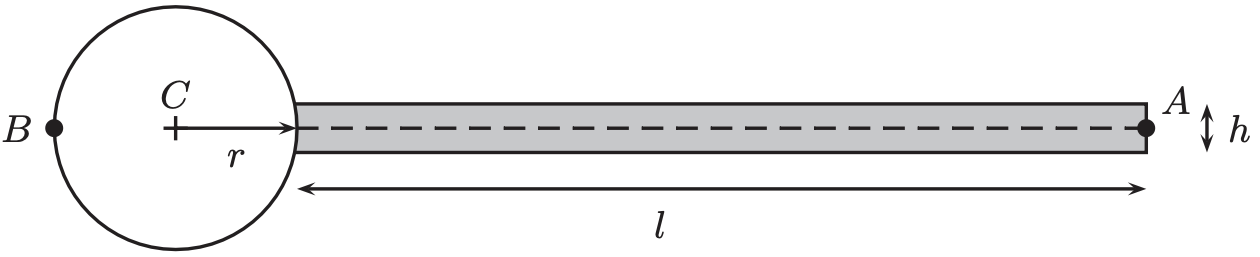
Figure 2: Computational domain of the FSI benchmark problem

We impose the no-slip boundary condition for the fluid velocity on $\Gamma_{walls}$ that include the surface of obstacle cylinder and the top and bottom walls of the channel domain, and do-nothing condition on the outlet $\Gamma_{out}$. In addition, we impose a parabolic profile of the incoming flow, i.e., the boundary condition of fluid velocity on the inlet $\Gamma_{in}$ is assigned to $({u}_{\text{in}},0)^{\top}$ such that

$${u}_{\text{in}}:=\left\{\begin{array}[]{ll}\hat{u}(y)\frac{1-\cos\left(\frac{\pi}{2}t\right)}{2},&\text{if }t<2s,\\ \hat{u}(y),&\text{otherwise, }\end{array}\right.$$ (24)

where $0\leq y\leq 0.41$ is the $y$-coordinate variable, and

$$\hat{u}(y)=\hat{U}\times\frac{4}{0.1681}y(0.41-y),$$ (25)

here the value of $\hat{U}$ is listed in Table 1, in which all other physical parameters of the FSI problem are reported as well. We also require the beam to be attached to the obstacle cylinder, therefore $\hat{\bm{d}}_{s}=0$ on $\Gamma_{walls}$. In what follows, all numerical computations are performed on a 12th-Gen Intel 3.20 GHz Core i9 computer.

Symbol	Description	Value	Unit
$\rho_{s}$	Density of the structure	$10^{4}$	$\frac{\mathrm{kg}}{\mathrm{m}^{3}}$
$\lambda_{s}$	Lamé constant of the structure	$0.4$	—
$\mu_{s}$	Shear modulus of the structure	$0.5\times 10^{6}$	$\frac{\mathrm{kg}}{\mathrm{ms}^{2}}$
$\rho_{f}$	Density of the fluid	$10^{3}$	$\frac{\mathrm{kg}}{\mathrm{m}^{3}}$
$\nu_{f}$	Kinematic viscosity of the fluid	$10^{-3}$	$\frac{\mathrm{m}^{2}}{\mathrm{s}}$
$\hat{U}$	The largest value of incoming fluid velocity	1.5	$\frac{\mathrm{m}}{\mathrm{s}}$

Table 1: Parameter settings for the FSI benchmark problem.

To verify the effectiveness of our developed ROM by comparing with FOM, we first perform the FOM computation for this FSI benchmark problem using the same time step size $\Delta t=0.001s$ as used in the benchmark problem proposed in [42, 43] on a fine triangular mesh with $18350$ degree of freedoms (DOFs) in total, as shown in Figure 3. Figure 4 illustrates the numerical result of vibration response at the location $A$ (the end of beam tail), where the vibration amplitude of point $A$ agrees with the benchmark result in [43] very well. As what we can observe in Figure 4, the vibrating frequency and amplitude stabilize after about 15 seconds. Therefore, we set the total simulation time $T=15s$ in the following tests.

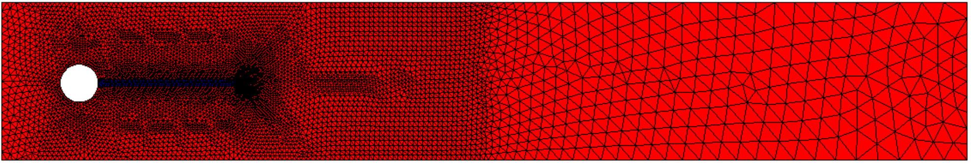
Figure 3: The triangular mesh of benchmark domain.

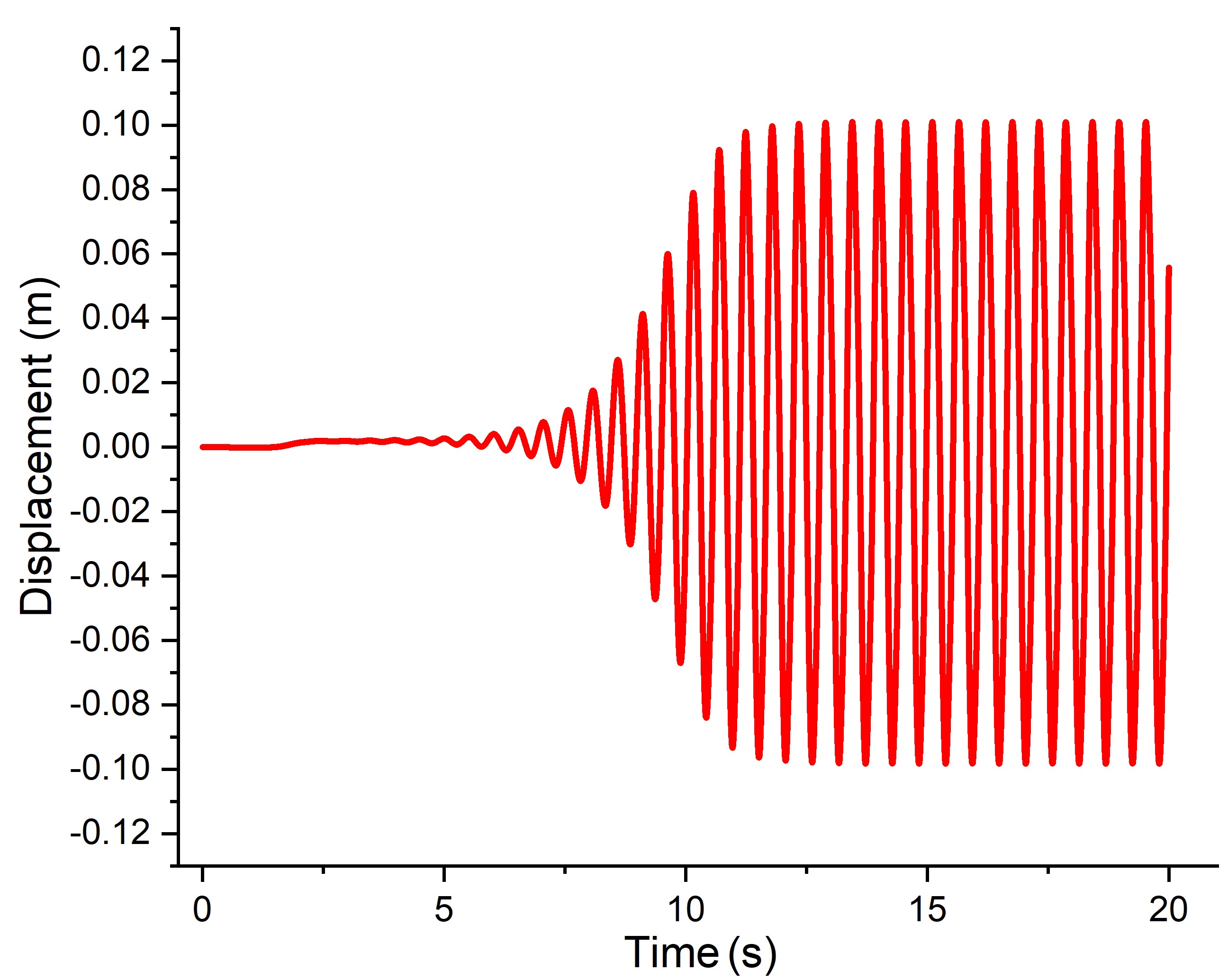
Figure 4: Vibration curve (the $y$-displacement trajectory) of point $A$ obtained from the FOM result.

4.1 Comparisons of FOM and ROM

In this subsection, we apply the ROM developed in Section 3 to solve the same FSI benchmark problem on the same mesh and with the same time step size $\Delta t=0.001s$. We do not reduce the order in the first two seconds, i.e., ROM is not used during the initial inflow buffer time $(t<2s)$. Thereafter, we divide the entire time interval $[2s,15s]$ into $130$ time segments with an equal width $0.1s$, and each time segment contains 100 time steps, i.e., there are $N_{T_{g}}=101$ time points in each $[T_{g},T_{g+1}]$ with a time step size $\Delta t=0.001s$, where $T_{g}=2+g*0.1$, $g=0,1,\cdots,129$. Then during the offline phase, in three time subintervals $[2s,6s]=\bigcup\limits_{g=0}^{39}[T_{g},T_{g+1}]$, $[6s,10s]=\bigcup\limits_{g=40}^{79}[T_{g},T_{g+1}]$, and $[10s,15s]=\bigcup\limits_{g=80}^{129}[T_{g},T_{g+1}]$ we construct the POD bases by choosing $N_{\bm{u}_{f}}=N_{\hat{\bm{d}}_{s}}=10,15$ and 20, and $N_{p_{f}}=30,40$ and 50, respectively, as illustrated in Figure 5. In particular, we let $N_{\hat{\bm{m}}_{f}}=N_{T_{g}}$ in each time subinterval here, which means we do not utilize the ROM but just the FOM to solve ALE mapping for the sake of ensuring the generated moving fluidic mesh shape-regular all the time.

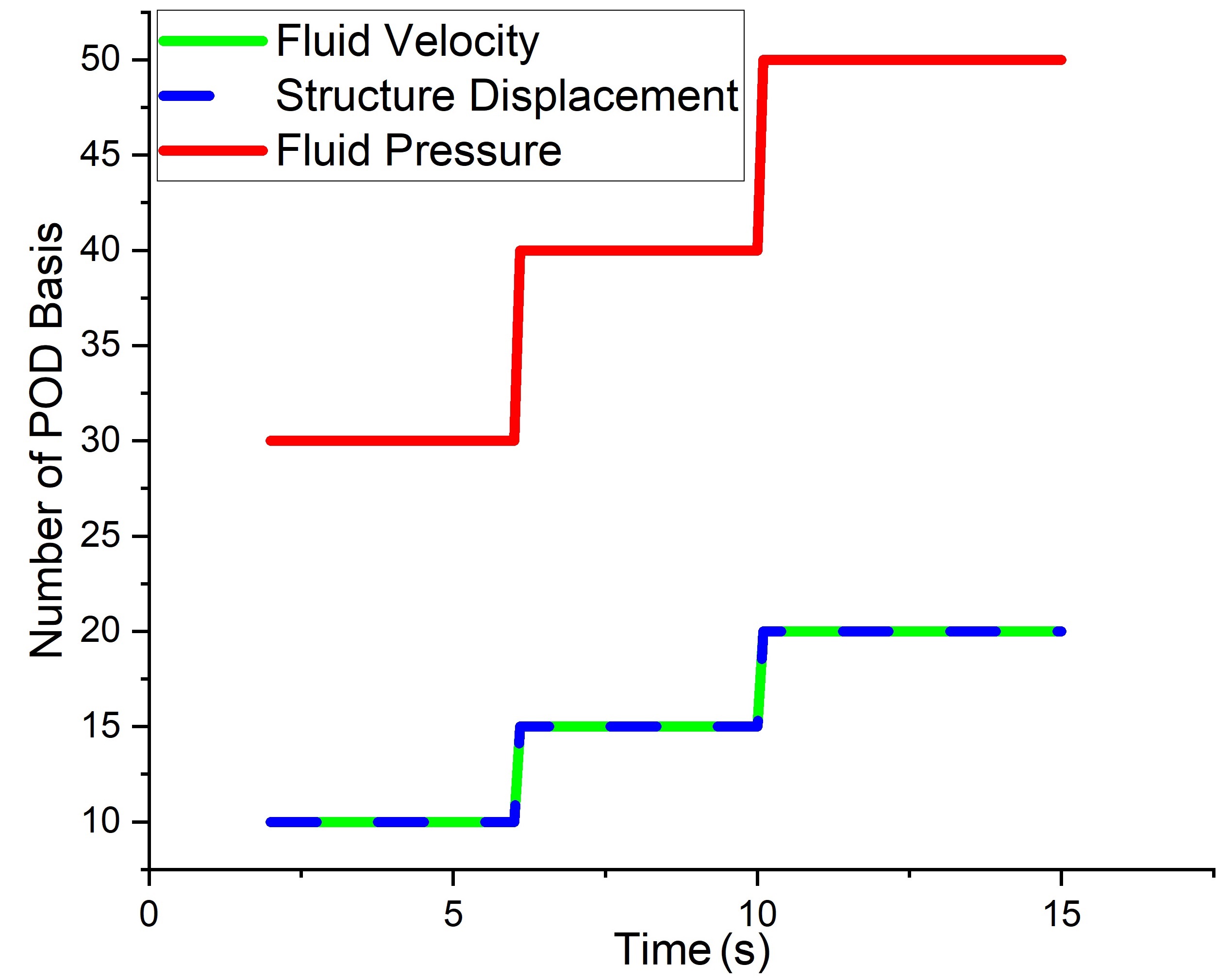
Figure 5: Number of POD bases’ selections over the time interval [2s,15s].

Then, we use the obtained POD basis to carry out the ROM for solving the FSI benchmark problem in each $[T_{g},T_{g+1}]\ (g=0,1,\cdots,129)$ during the online phase, where the ROM solution obtained by reducing the order at the end of the previous time segment $[T_{g-1},T_{g}]$ is adopted as the initial value at the starting point of the current time segment $[T_{g},T_{g+1}]$. Specifically, the case of $g=0$ is referred to the last paragraph of Section 3.2. Finally, we attain the solution of ROM over the entire time period $[0,15s]$.

In the following, we introduce the proportion of eigenvalues, $\frac{\sum_{k=1}^{{N}_{*}}\lambda_{k}^{*}}{\sum_{k=1}^{{N}_{T_{g}}}\lambda_{k}^{*}}$, where $*\in\{\bm{u}_{f},p_{f},\hat{\bm{d}}_{s}\}$ and $\lambda_{k}^{*}$ denotes the $k$-th eigenvalue of $\mathcal{C}_{*}$ in $[T_{g},T_{g+1}]$, to demonstrate the proportion of the sum of all selected eigenvalues amongst the sum of all eigenvalues in each time segment. We further introduce the following three error indicators that are used later to compare numerical results between the FOM and ROM:

1. The relative spatial $L^{2}$ error between the FOM solution $\bm{U}_{g}^{n}$ and the ROM solution $\mathbf{u}_{h}^{n,rom}$, $\frac{\|\bm{U}_{g}^{n}-\mathbf{u}_{h}^{n,rom}\|_{L^{2}(\Omega)}}{\|\bm{U}_{g}^{n}\|_{L^{2}(\Omega)}}$;

2. The relative spatio-temporal $L^{2}$ error between the FOM solution $\bm{U}_{g}^{n}$ and the ROM solution $\mathbf{u}_{h}^{n,rom}$, $\frac{\|\bm{U}_{g}^{n}-\mathbf{u}_{h}^{n,rom}\|_{L^{2}(0,T;L^{2}(\Omega))}}{\|\bm{U}_{g}^{n}\|_{L^{2}(0,T;L^{2}(\Omega))}}$;

3. The absolute error of $y$-displacement of point $A$ between the FOM result $Dy_{fom}$ and the ROM result $Dy_{rom}$, expressed as $(Dy_{fom}-Dy_{rom})$.

Figure 6 shows the eigenvalue changes associated with three variables: fluid velocity, fluid pressure and structural displacement within several typical time segments. Through Figure 6 we intend to reveal the following fact that in each time segment $[T_{g},T_{g+1}]$, these $N_{T_{g}}$ vectors, $\left(\bm{U}_{g}^{1},\bm{U}_{g}^{2},\cdots,\bm{U}_{g}^{N_{T_{g}}}\right)$, are linearly dependent, leading to a low-rank snapshot matrix $\bm{U}_{g}$, which explains why ROM works in this scenario [34]. Figure 7 illustrates proportions of eigenvalues of the first 10 eigenvalues that are associated with three variables within several typical time segments, which helps us to determine how many POD bases need to be selected for each variable, at least. In addition, from Figures 6 and 7 we also observe the following facts:

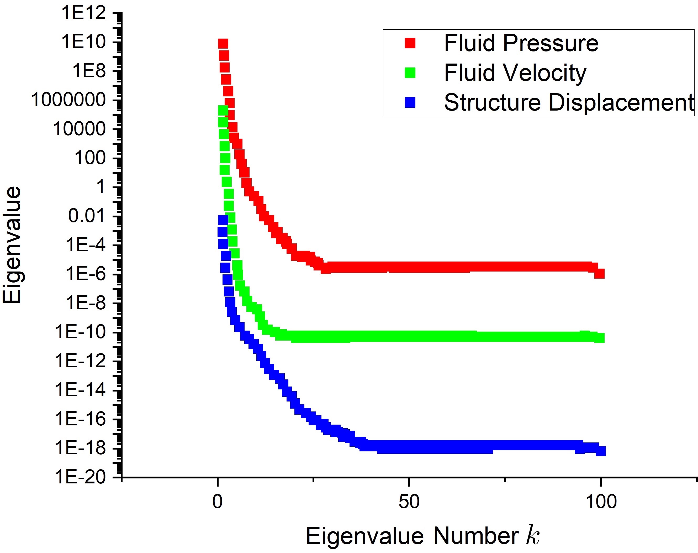
(a) $2.0\sim 2.1s$

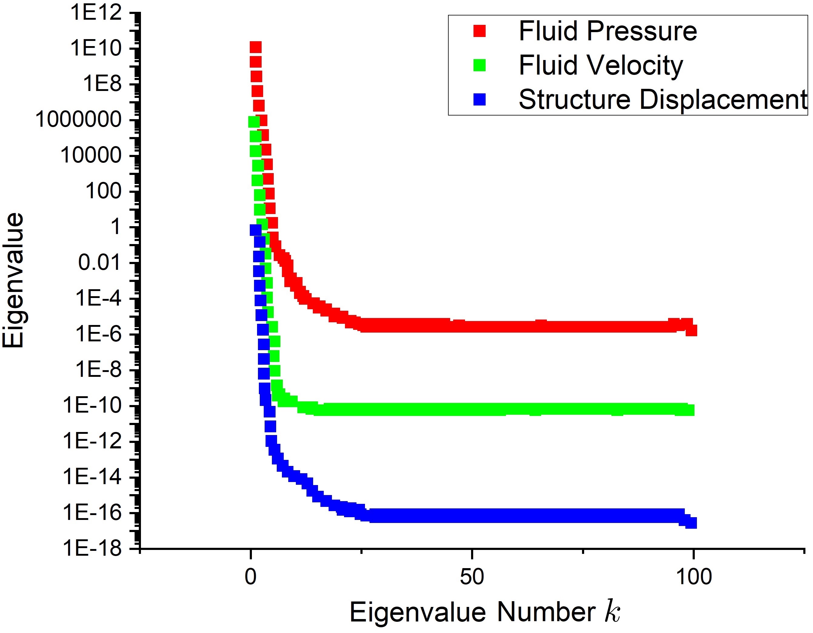
(b) $6.0\sim 6.1s$

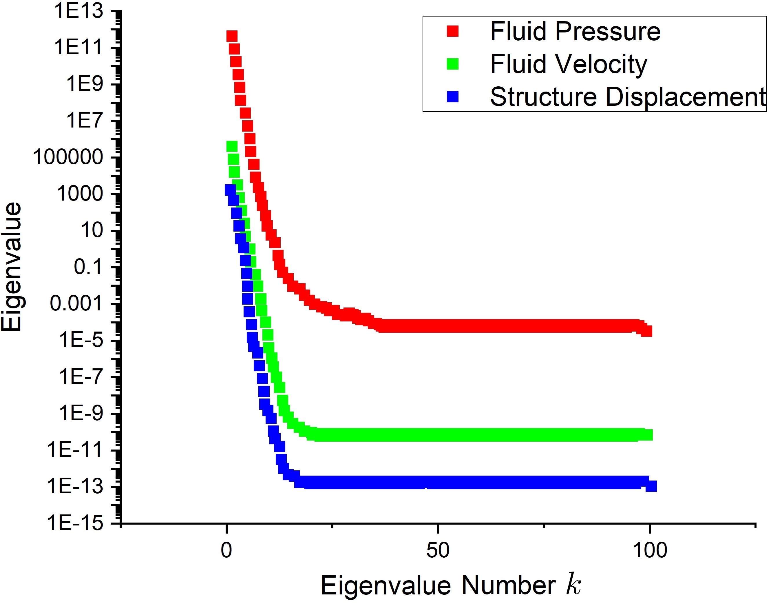
(c) $10.0\sim 10.1s$

Figure 6: History of eigenvalue decay within typical time segments

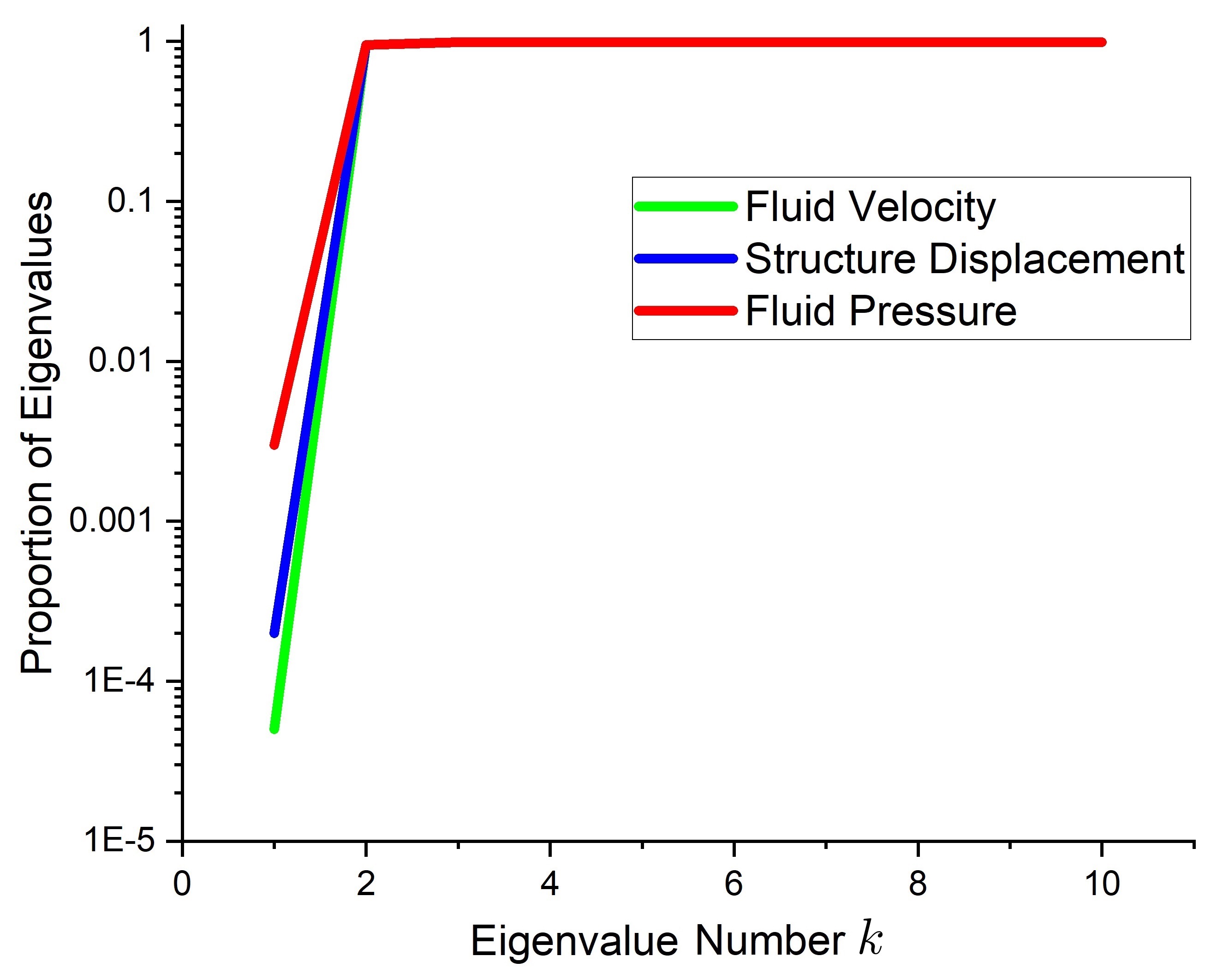
(a) $2.0\sim 2.1s$

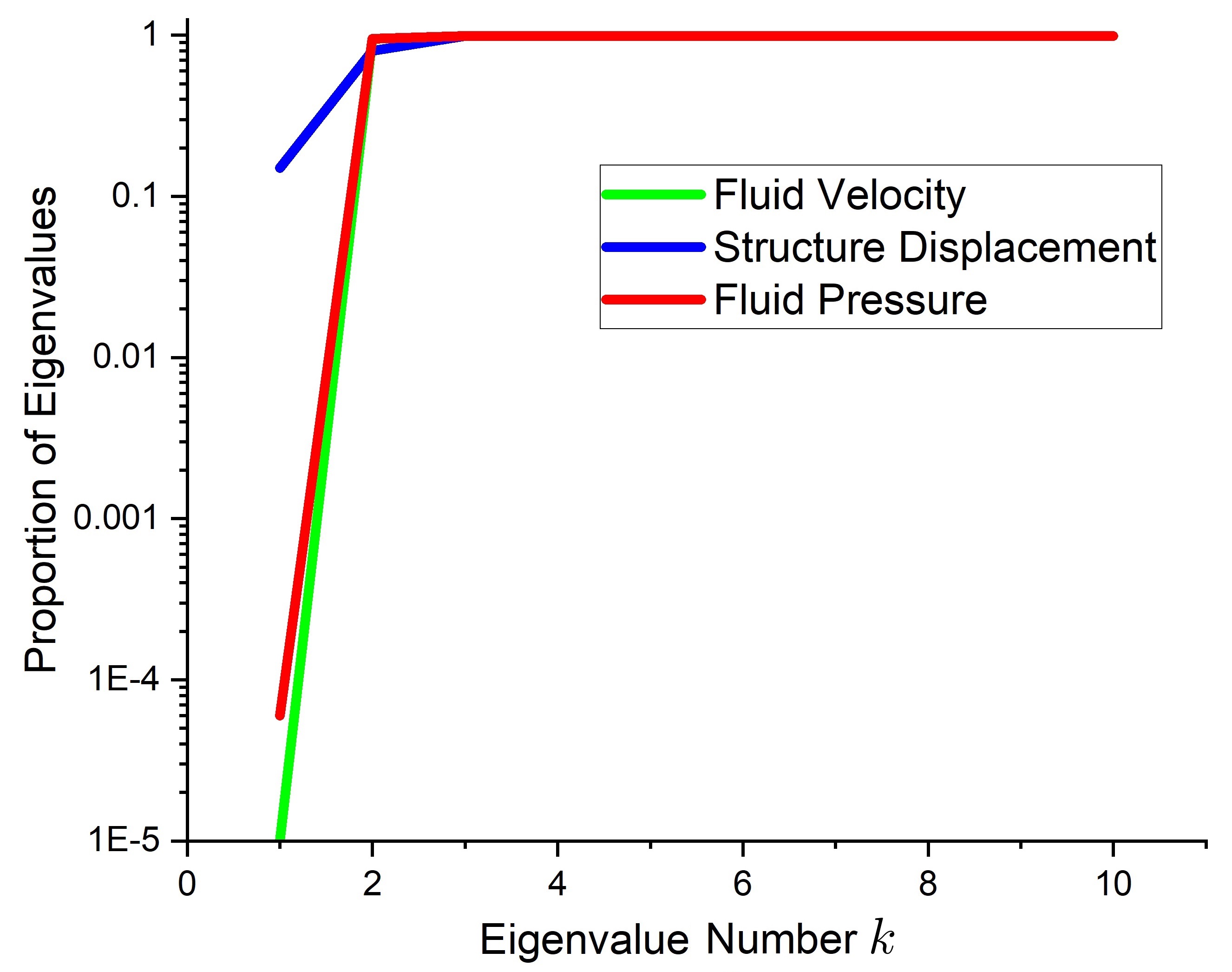
(b) $6.0\sim 6.1s$

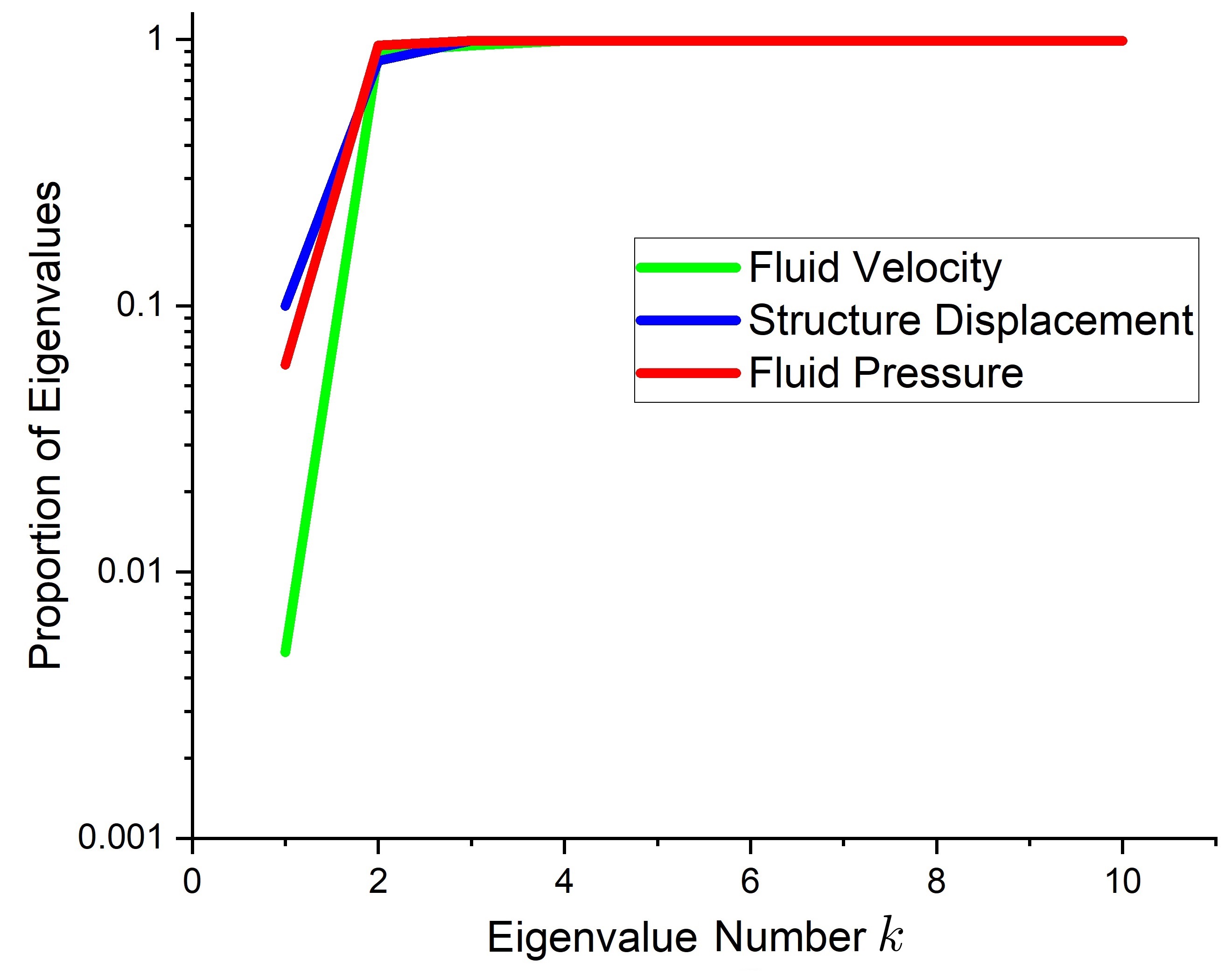
(c) $10.0\sim 10.1s$

Figure 7: History of proportion of eigenvalues within typical time segments

• Within the same time period, the eigenvalue decay rates of both fluid velocity and fluid pressure are closer to each other, while they are significantly slower than that of the structural displacement;

• The eigenvalue decay rates of all variables slow down when time marches (i.e., the eigenvalue number grows);

• When the number of POD bases is chosen larger than 5, proportions of eigenvalues for different variables are all close to 1;

• The eigenvalue number with high proportion increases with time, i.e., the bigger eigenvalue number, the higher proportion of eigenvalues.

Table 2 shows the comparison between the FOM and ROM in terms of the number of DOFs and computational time during different time periods, where the computational time is the time taken to solve the linear algebraic system during that time period. We can see that the ROM greatly saves the computational time for almost $100\%$ corresponding to the FOM, and averagely speed up the linear algebraic solver 8844 times, which is a huge improvement on the computational efficiency.

Time subinterval	$2\sim 6s$	$6\sim 10s$	$10\sim 15s$
# of DOFs of FOM	18350	18350	18350
# of DOFs of ROM	50	70	90
Reduction Rate in # of DOFs	367:1	263:1	204:1
Comput. Time of FOM (s)	$5.52\times 10^{4}$	$5.52\times 10^{4}$	$6.91\times 10^{4}$
Comput. Time of ROM (s)	5.62	6.25	8.77
Reduction Rate in Comput. Time	99.990%	99.989%	99.987%
Speedup	$9.822\times 10^{3}$	$8.832\times 10^{3}$	$7.879\times 10^{3}$

Table 2: Numerical comparison between the FOM and ROM in terms of # of DOFs and computational time during different time periods.

In regard to the numerical accuracy of ROM versus that of FOM, we investigate solution errors between the ROM and FOM shown in Figures 8-10, and observe the following numerical phenomena:

• The vibration curve of the beam tail end, i.e., the $y$-displacement of point $A$ with time, has a good match with that of the FOM, and the error $(Dy_{fom}-Dy_{rom})$ is well controlled within $\pm 0.002$;

• The contour snapshots of velocity and fluid pressure at T=15s are similar between the FOM and ROM. The total relative spatial $L^{2}$ error is well controlled within $0.01$;

• The relative spatial $L^{2}$ error of fluid pressure is similar to the total relative spatial $L^{2}$ error, while that of fluid velocity and structural displacement are slightly smaller than the total relative spatial $L^{2}$ error, meaning that the ROM approximation to the fluid pressure is less accurate than that to the fluid velocity and structural displacement.

• As time marches, errors also grow. But as the beam vibration stabilizes, the relative spatial $L^{2}$ errors for all variables finally stabilize;

• The relative spatio-temporal $L^{2}$ error is $0.0056$.

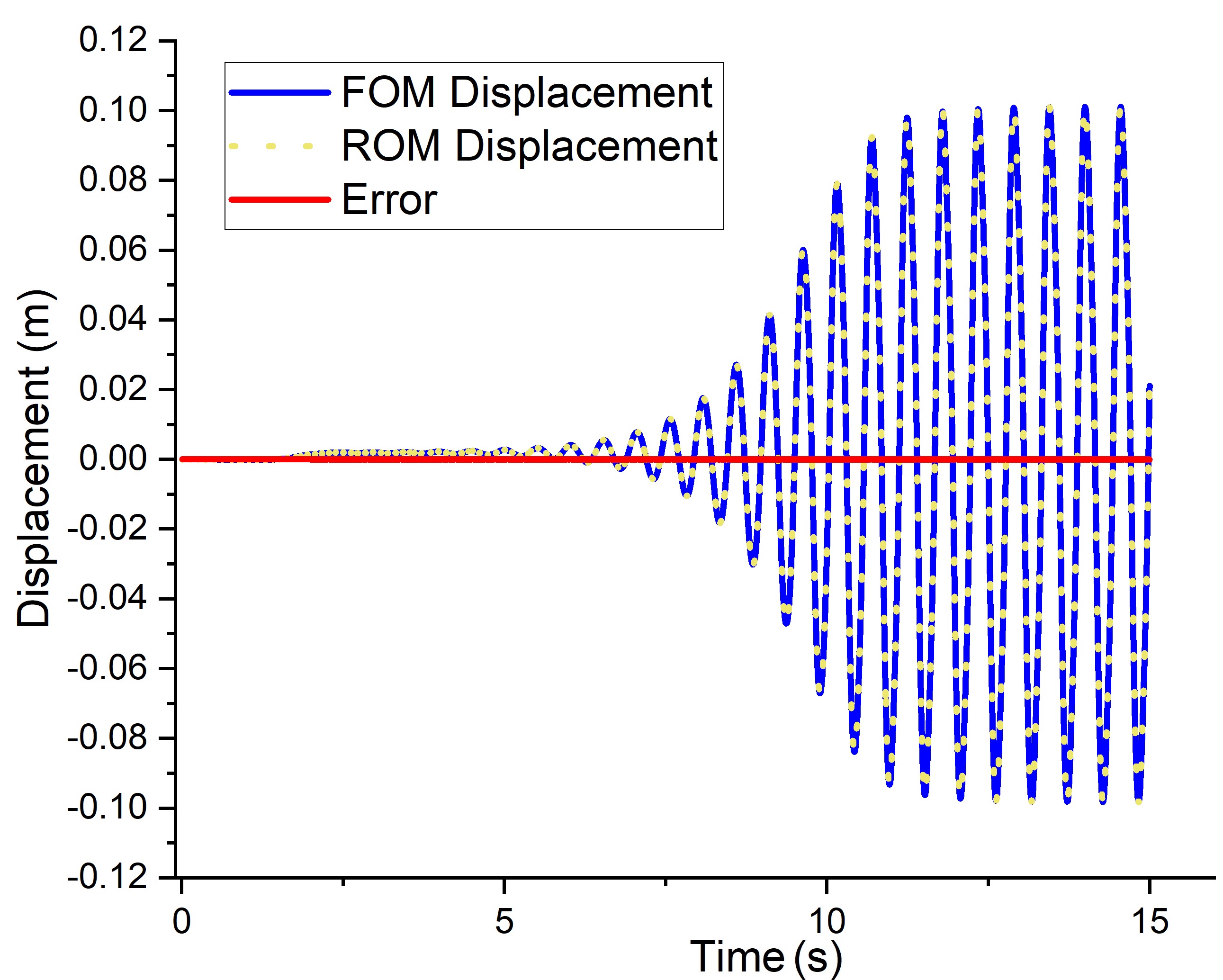
Figure 8: Blue solid: the $y$-displacement curve of FOM at point $A$; Yellow dot:the $y$-displacement curve of ROM at point $A$; Red solid: Error curve of $y$-displacement at point $A$ between FOM and ROM, $Dy_{fom}-Dy_{rom}$, over the entire time interval.

(a) Horizontal velocity of FOM

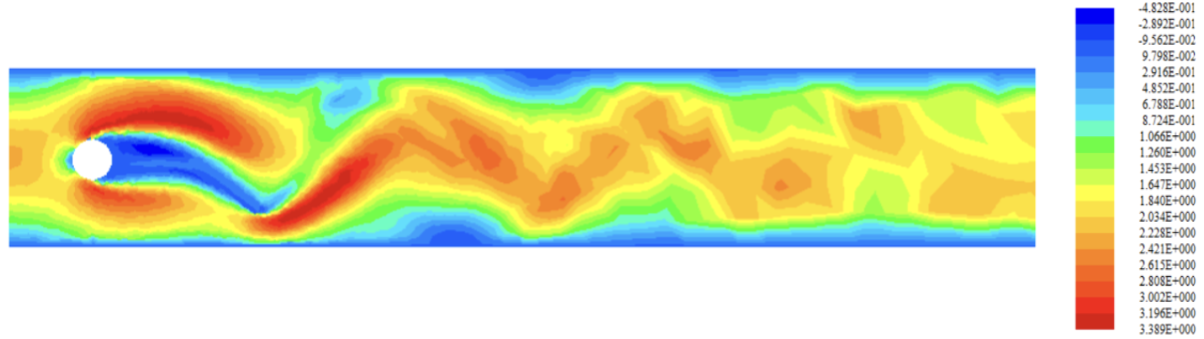
(b) Horizontal velocity of ROM

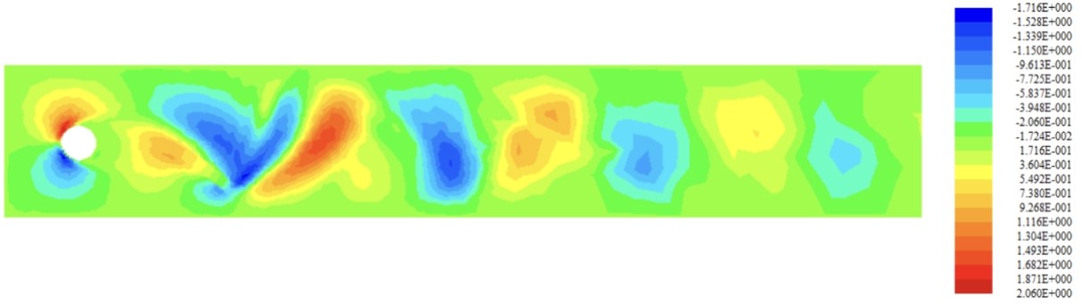
(c) Vertical velocity of FOM

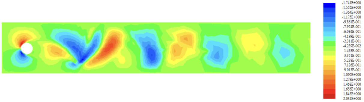
(d) Vertical velocity of ROM

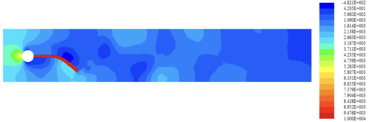
(e) Fluid pressure of FOM

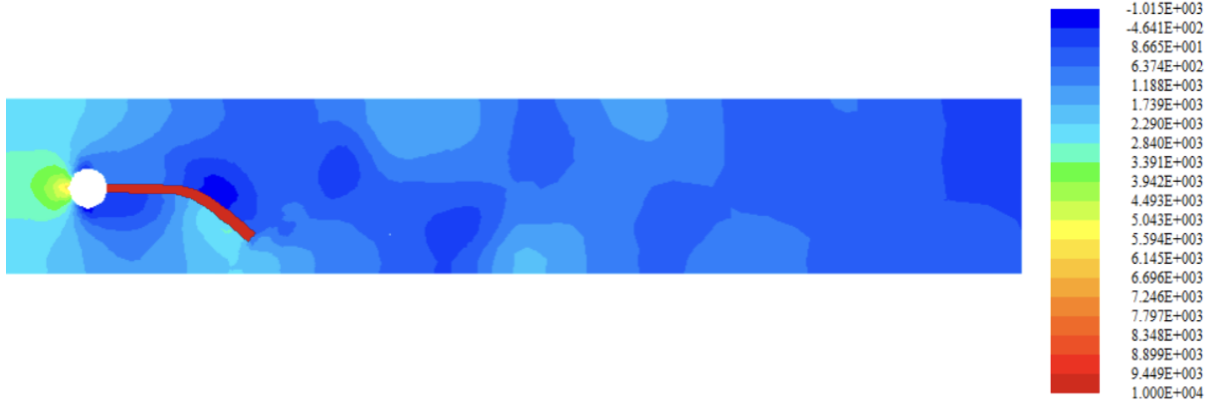
(f) Fluid pressure of ROM

Figure 9: FSI solutions between FOM and ROM at the terminal time $t=15s$.

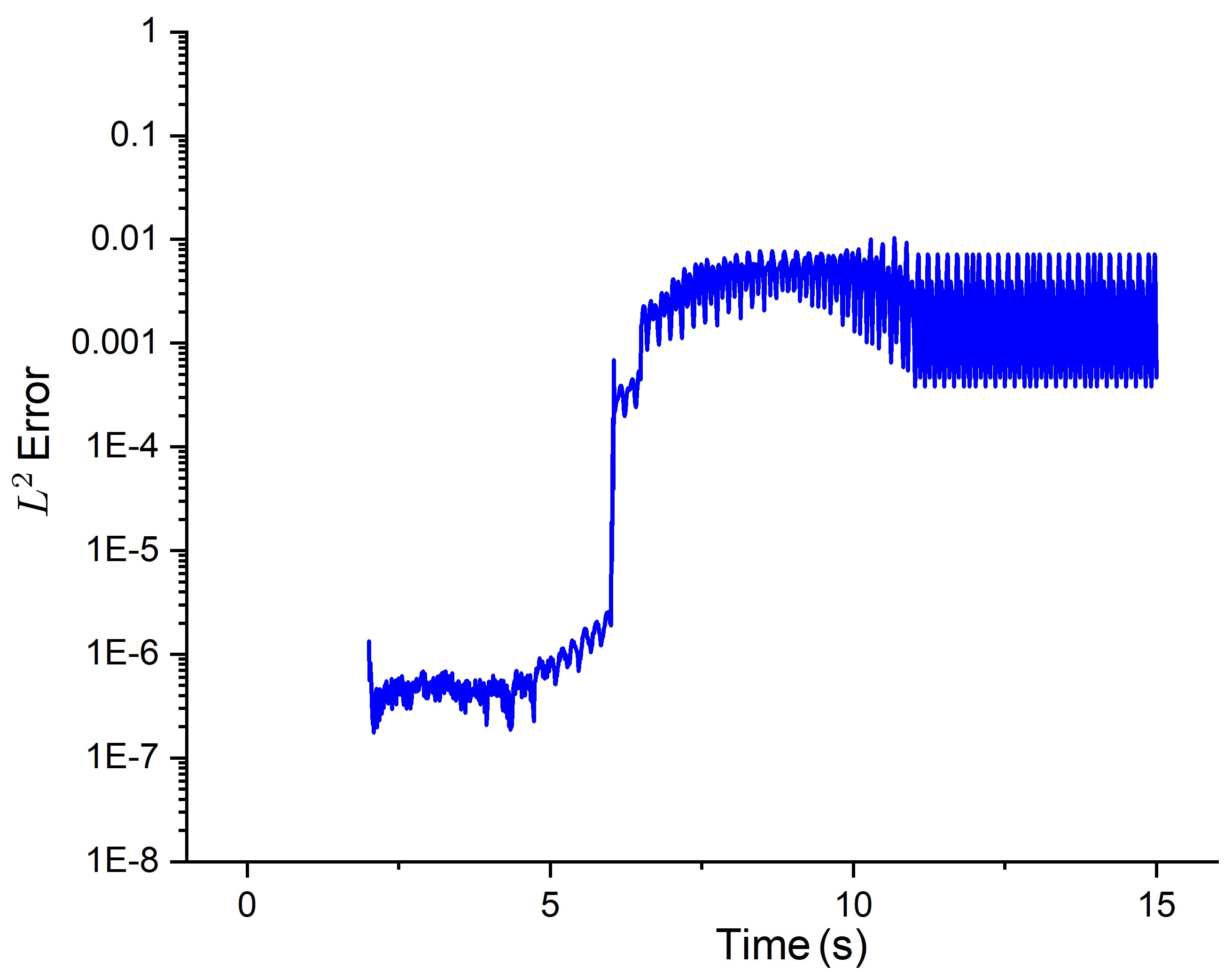
(a) Total error.

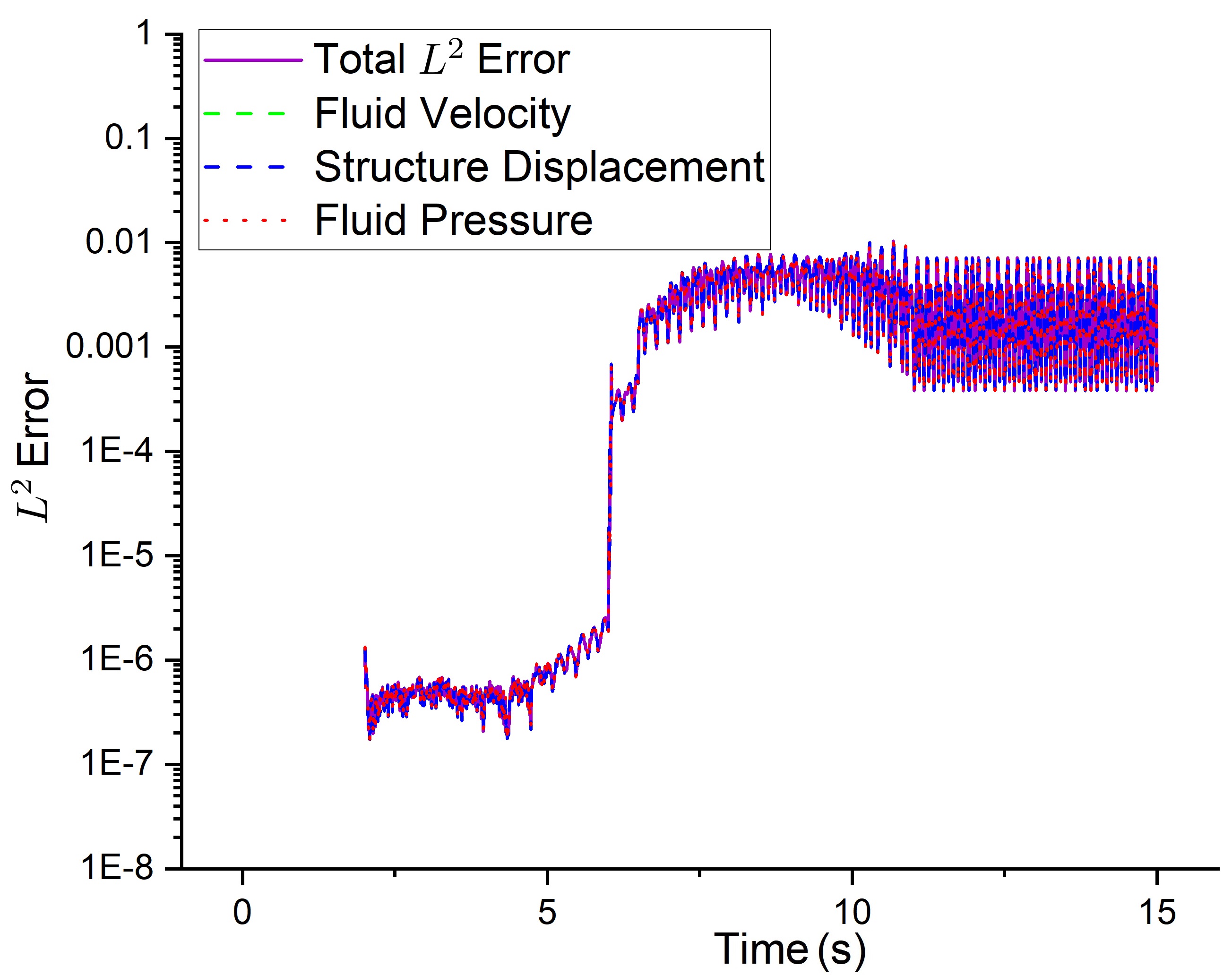
(b) Errors of all individual variables combining with total error.

Figure 10: Relative spatial $L^{2}$ errors between ROM and FOM over the entire time interval.

Next, we test whether the constructed POD basis can let the developed ROM have a good approximation to the FOM when physical parameters are perturbed in a reasonable range. Without loss of generality, we choose to change the maximum incoming fluid velocity, $\hat{U}$, for the fluid part and the Young’s modulus, $\mu_{s}$, for the structure part. While keeping all the other parameters unchanged, we perturb $\hat{U}=1.5$ by $\pm\,0.02$ , or $\mu_{s}=0.5\times 10^{6}$ by $\pm\,0.02\times 10^{6}$, i.e., we let $\hat{U}=1.52$ or $1.48$, $\mu_{s}=0.52\times 10^{6}$ or $0.48\times 10^{6}$, respectively, resulting in four testing cases in total. Figures 11-22 show corresponding results of FOM and ROM, and of their comparison errors under these four scenarios, from which we can observe the following numerical phenomena:

• The POD bases generated at $\hat{U}=1.5$ , $\mu_{s}=0.5\times 10^{6}$ have a certain degree of generalization ability, and can reproduce relatively high-fidelity solutions even if physical parameters are slightly changed in all cases;

• The error of $y$-displacement at point $A$, $(Dy_{fom}-Dy_{rom})$, is well controlled within $\pm 0.01$ and gradually stabilizes along with the stabilization of beam vibration for all cases;

• The contour snapshots of velocity and fluid pressure at T=15s are similar between the FOM and ROM. The total relative spatial $L^{2}$ error is well controlled around $0.1$, and gradually stabilizes along with the stabilization of vibration for all cases.

• As time marches, errors also grow. But as the beam vibration stabilizes, the relative spatial $L^{2}$ errors for all variables gradually stabilize for all cases.

• The relative spatio-temporal $L^{2}$ errors for all cases are displayed below: (1) Case $\hat{U}=1.52$: 0.0632; (2) Case $\hat{U}=1.48$: 0.0421; (3) Case $\mu_{s}=0.52\times 10^{6}$: 0.0387; (4) Case $\mu_{s}=0.48\times 10^{6}$: 0.0394. In summary, all relative spatio-temporal $L^{2}$ errors are well controlled around $0.0459$, on the average.

Figure 11: Error of $y$-displacement at point $A$ between FOM and ROM for Case $\hat{U}=1.52$.

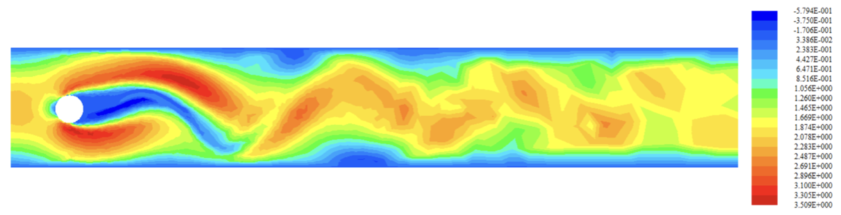
(a) Horizontal velocity of FOM

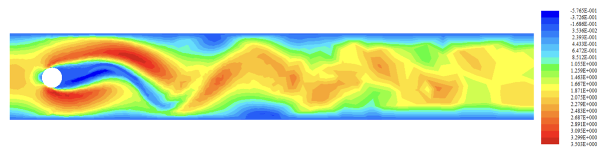
(b) Horizontal velocity of ROM

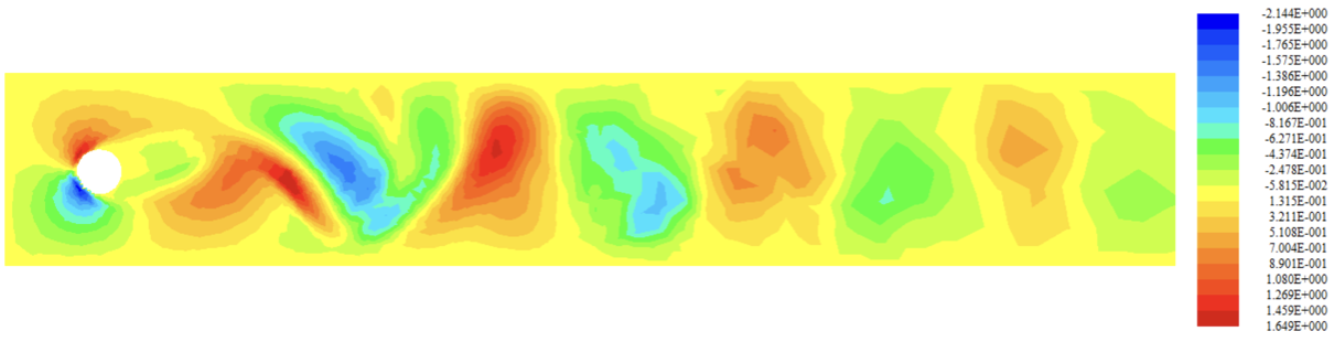
(c) Vertical velocity of FOM

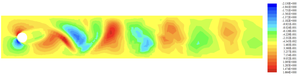
(d) Vertical velocity of ROM

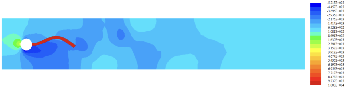
(e) Fluid pressure of FOM

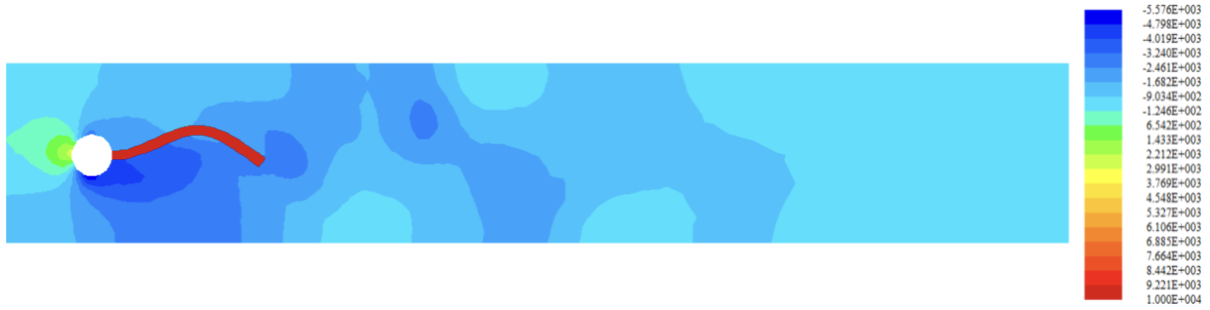
(f) Fluid pressure of ROM

Figure 12: FSI solutions between FOM and ROM at the finial time $t=15s$ for Case $\hat{U}=1.52$.

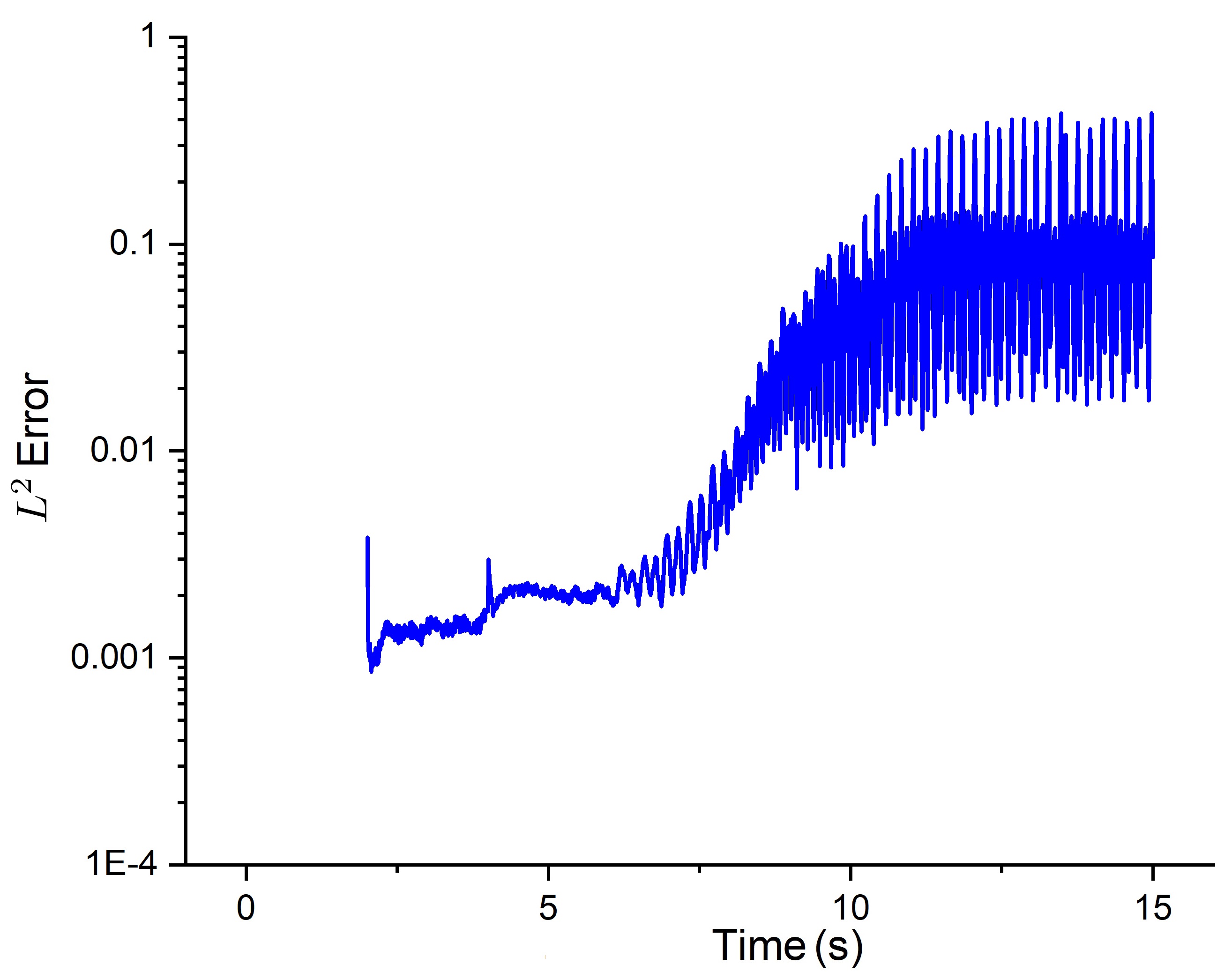
(a) Total error.

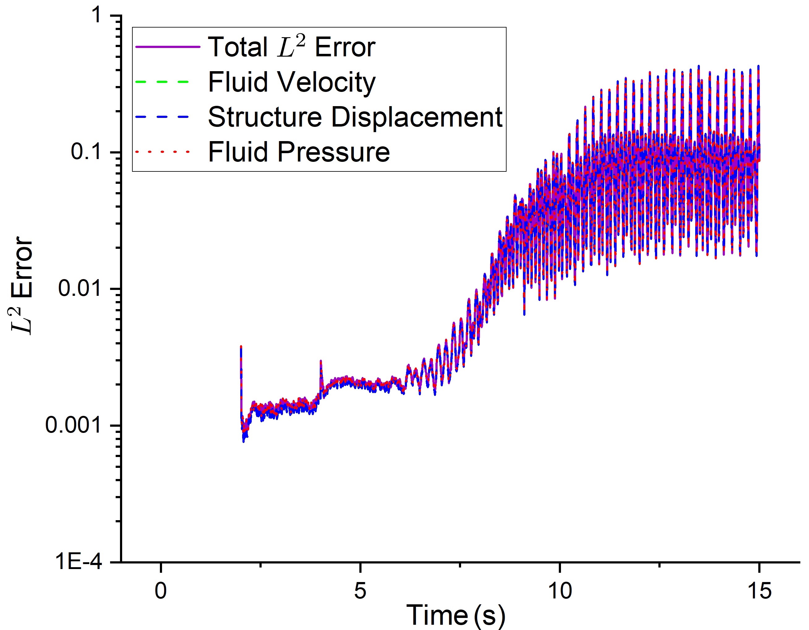
(b) Errors of all individual variables combining with total error.

Figure 13: Relative spatial $L^{2}$ errors between ROM and FOM over the entire time interval for Case $\hat{U}=1.52$.

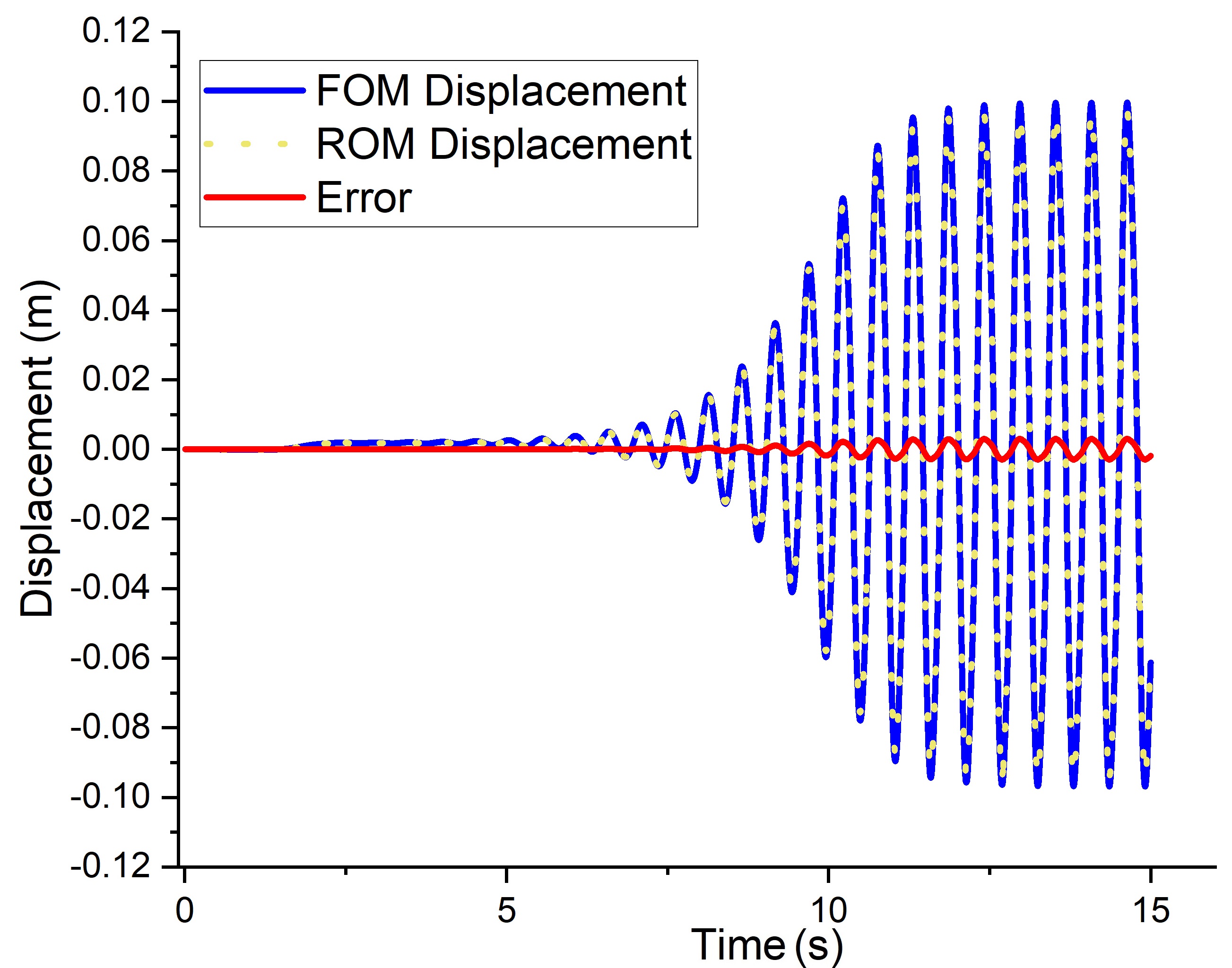
Figure 14: Error of $y$-displacement at point $A$ between FOM and ROM for Case $\hat{U}=1.48$.

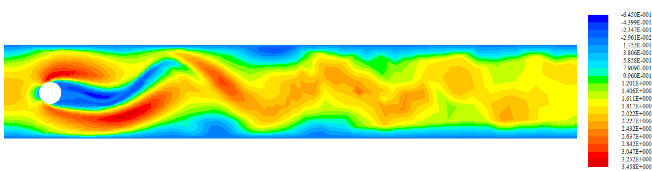
(a) Horizontal velocity of FOM

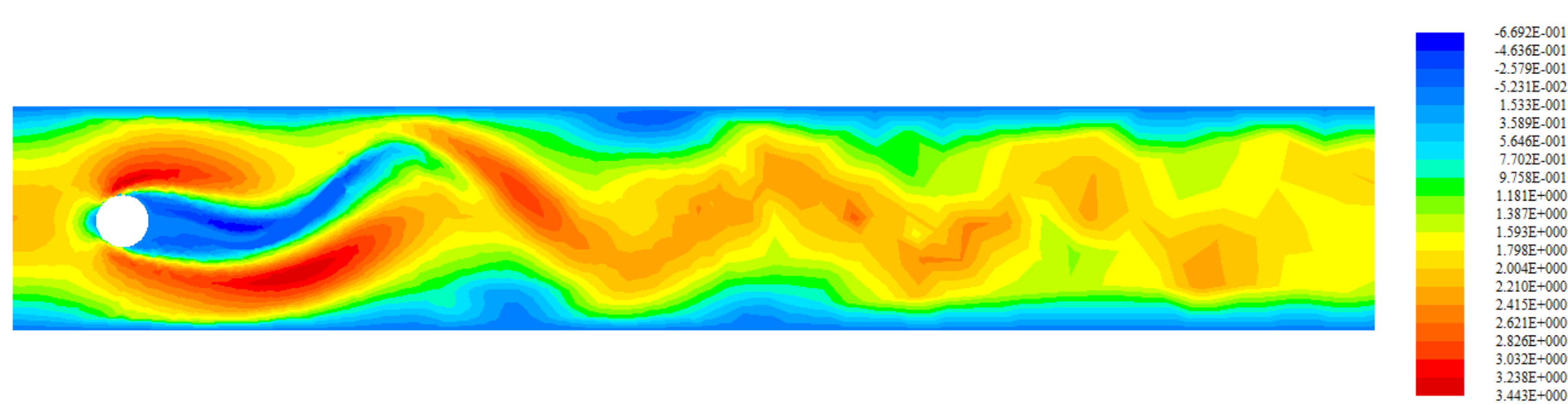
(b) Horizontal velocity of ROM

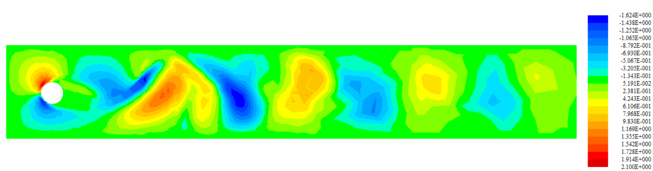
(c) Vertical velocity of FOM

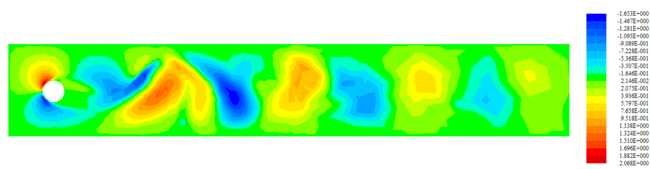
(d) Vertical velocity of ROM

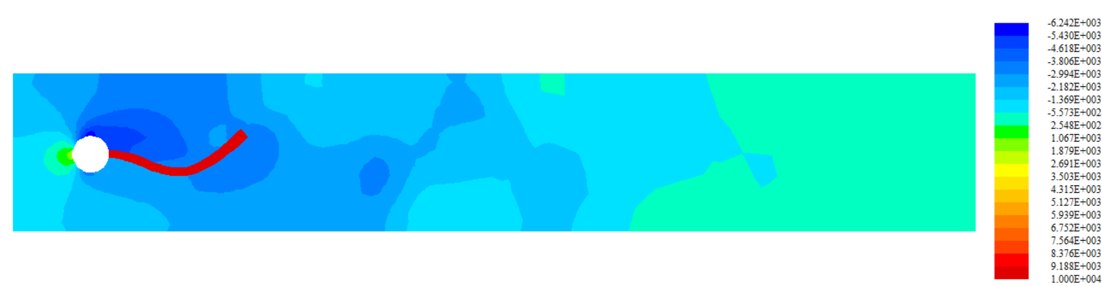
(e) Fluid pressure of FOM

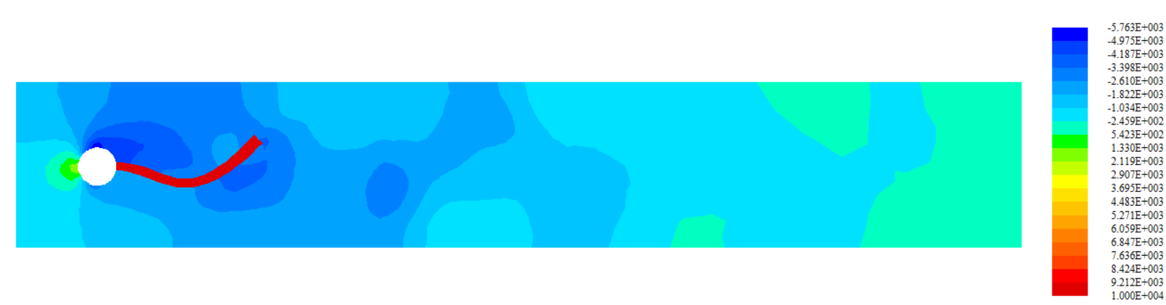
(f) Fluid pressure of ROM

Figure 15: FSI solutions between FOM and ROM at the finial time $t=15s$ for Case $\hat{U}=1.48$.

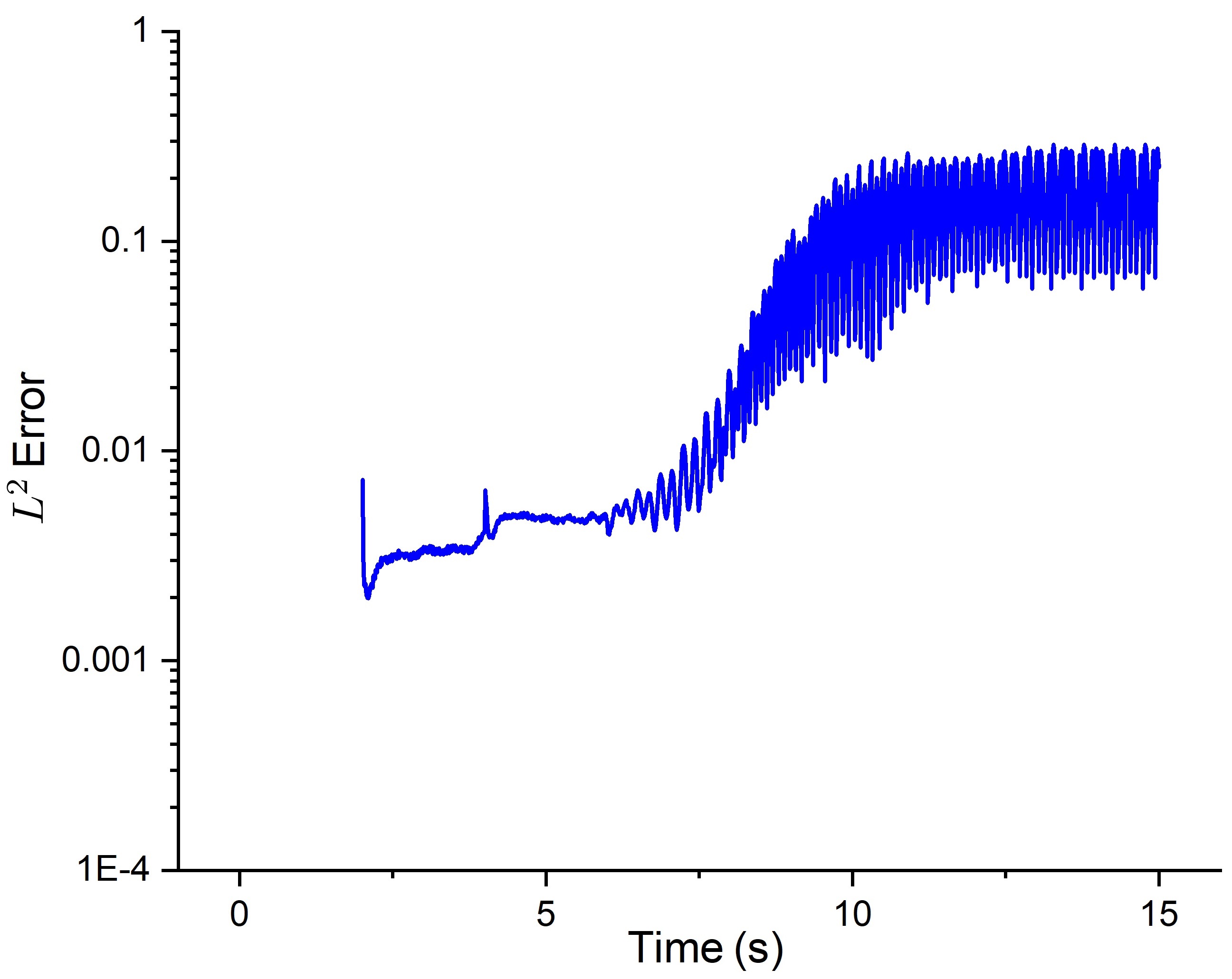
(a) Total error.

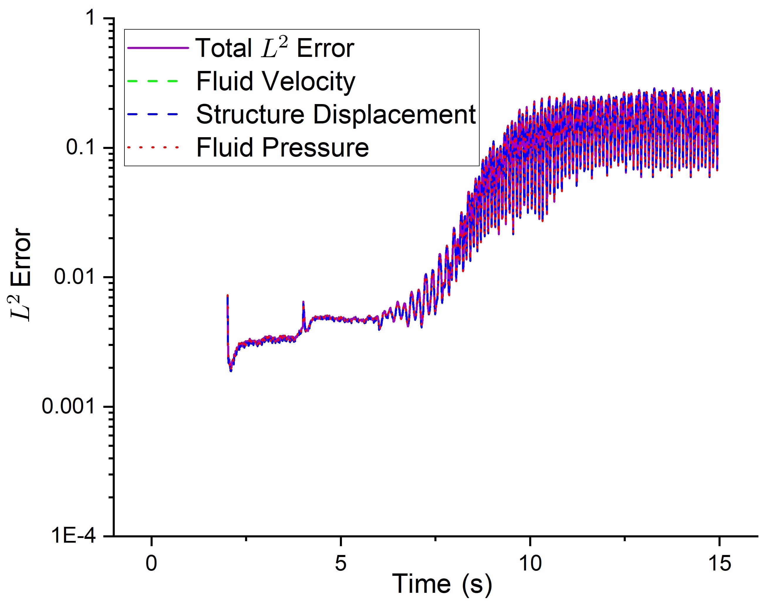
(b) Errors of all individual variables combining with total error.

Figure 16: Relative spatial $L^{2}$ errors between ROM and FOM over the entire time interval for Case $\hat{U}=1.48$.

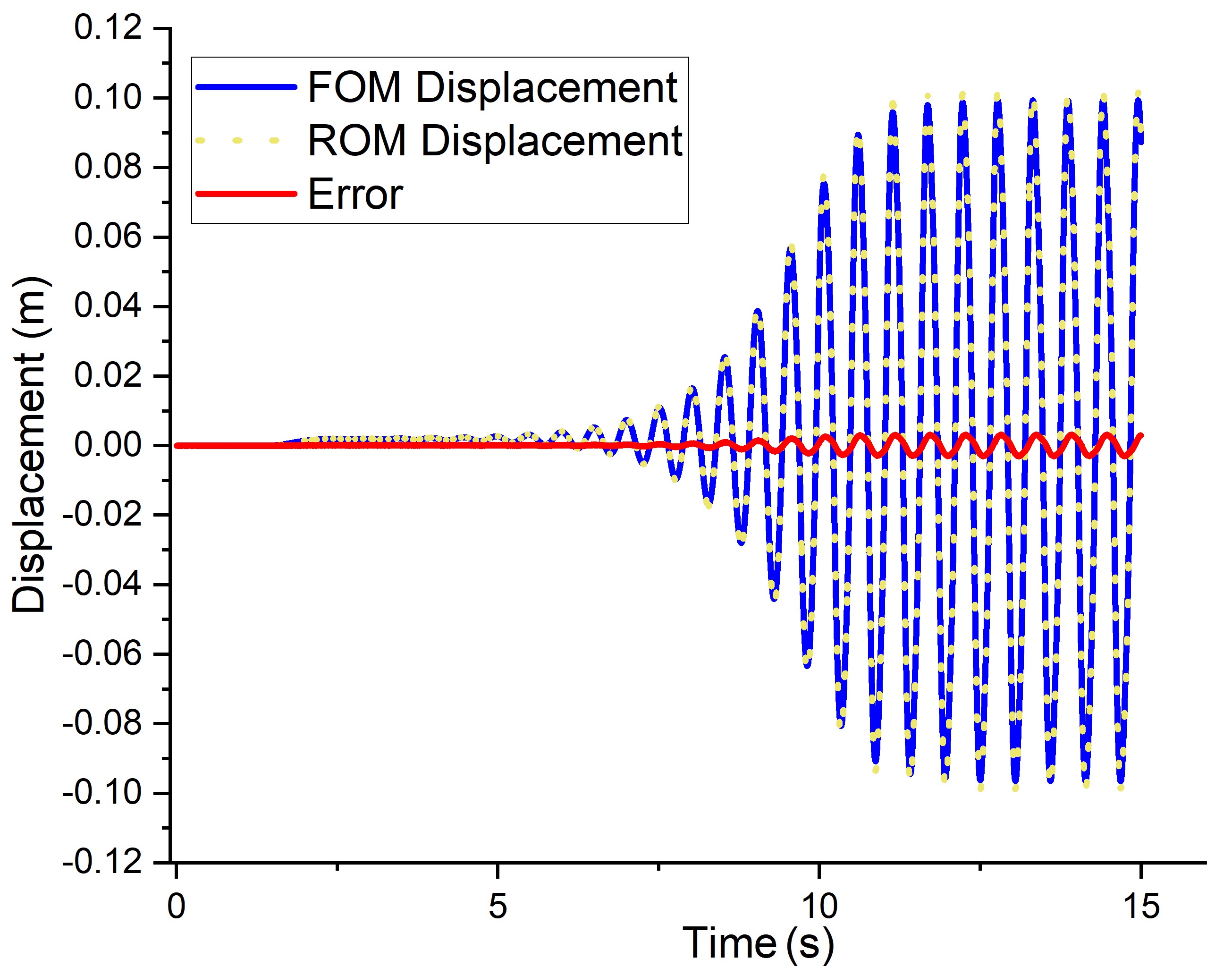
Figure 17: Error of $y$-displacement at point $A$ between FOM and ROM for Case $\mu_{s}=0.52\times 10^{6}$.

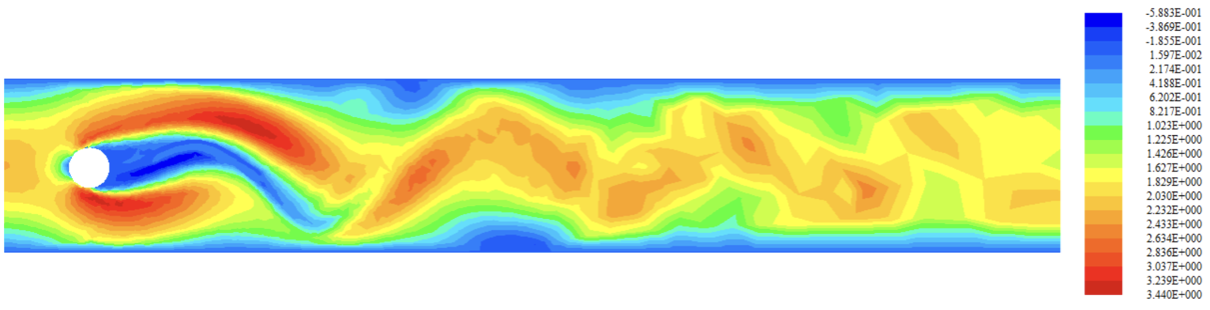
(a) Horizontal velocity of FOM

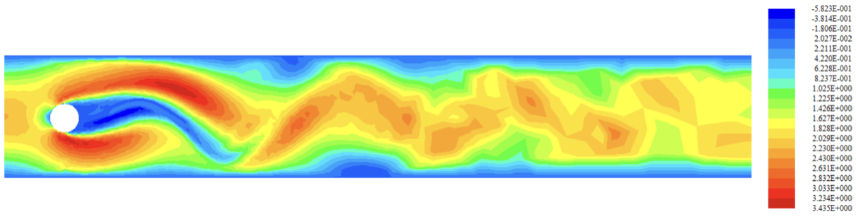
(b) Horizontal velocity of ROM

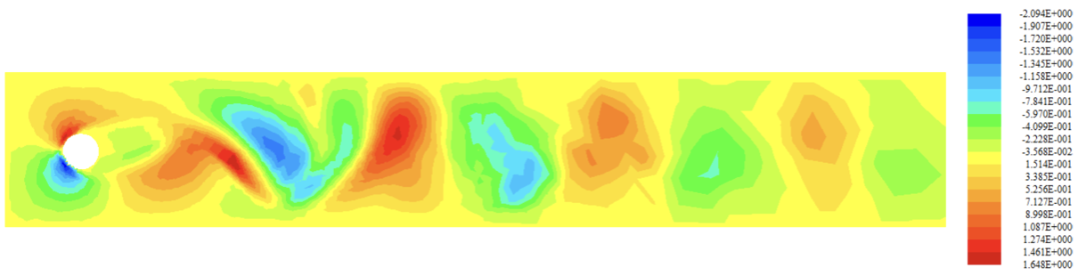
(c) Vertical velocity of FOM

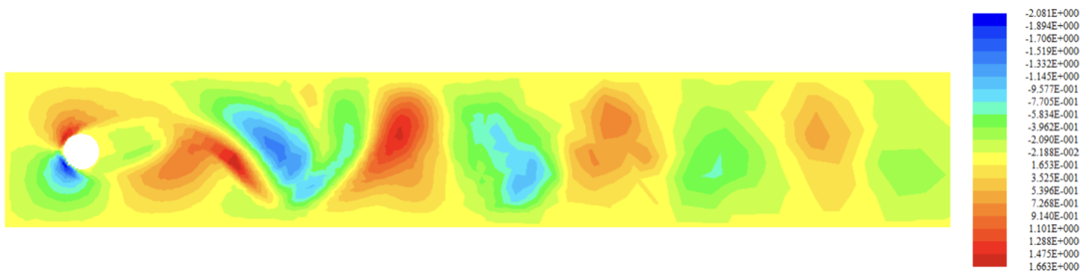
(d) Vertical velocity of ROM

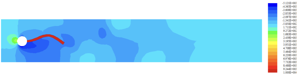
(e) Fluid pressure of FOM

(f) Fluid pressure of ROM

Figure 18: FSI solutions between FOM and ROM at the finial time $t=15s$ for Case $\mu_{s}=0.52\times 10^{6}$.

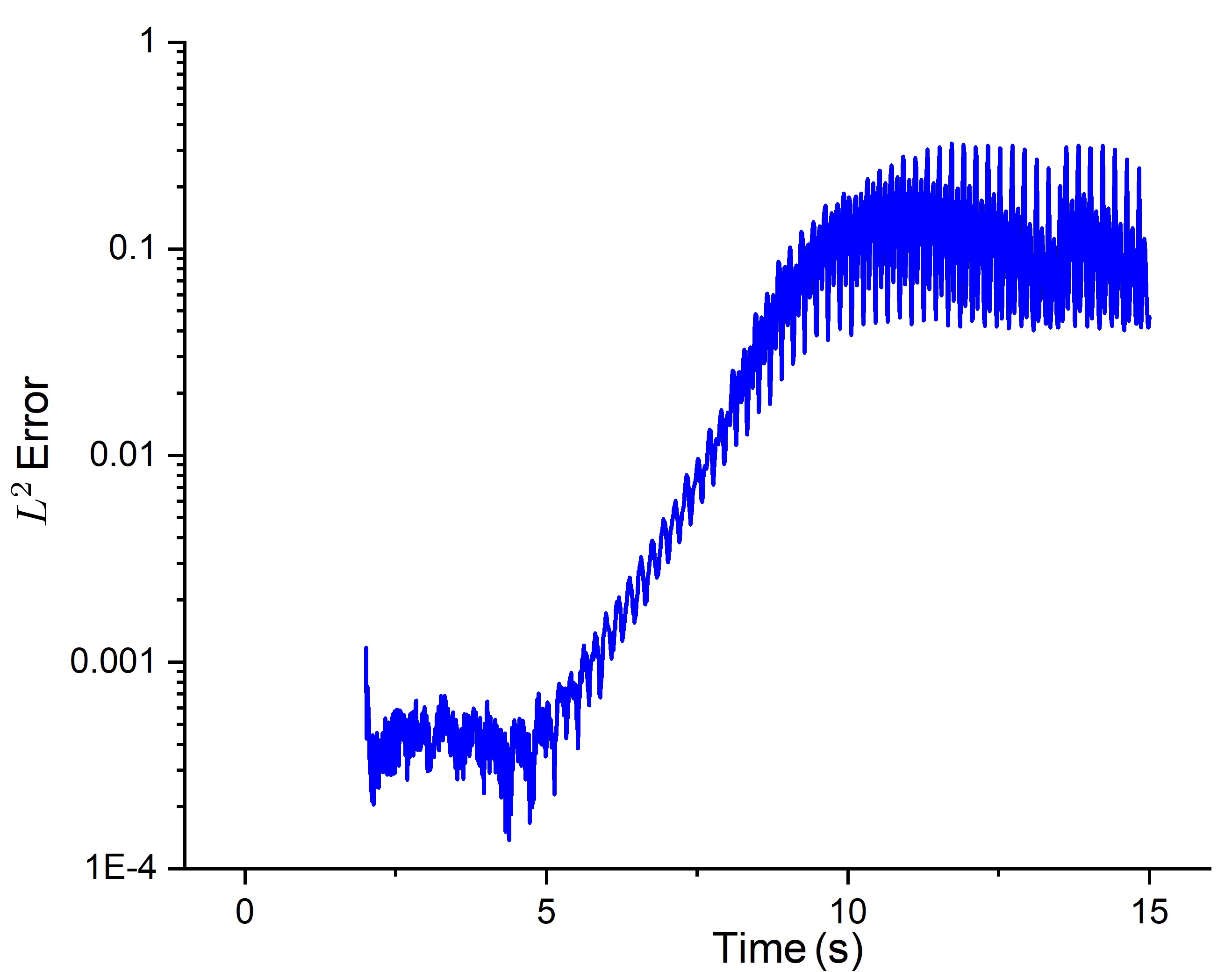
(a) Total error.

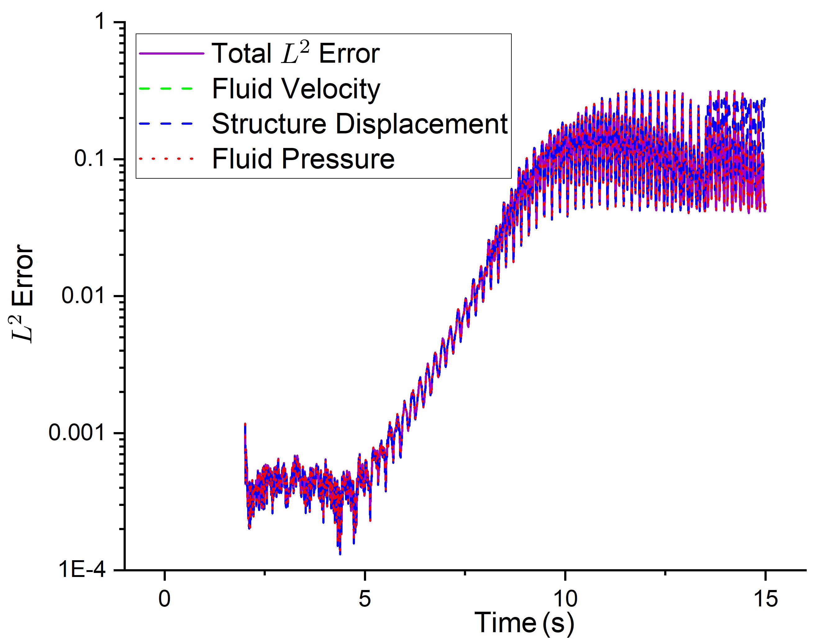
(b) Errors of all individual variables combining with total error.

Figure 19: Relative spatial $L^{2}$ errors between ROM and FOM over the entire time interval for Case $\mu_{s}=0.52\times 10^{6}$.

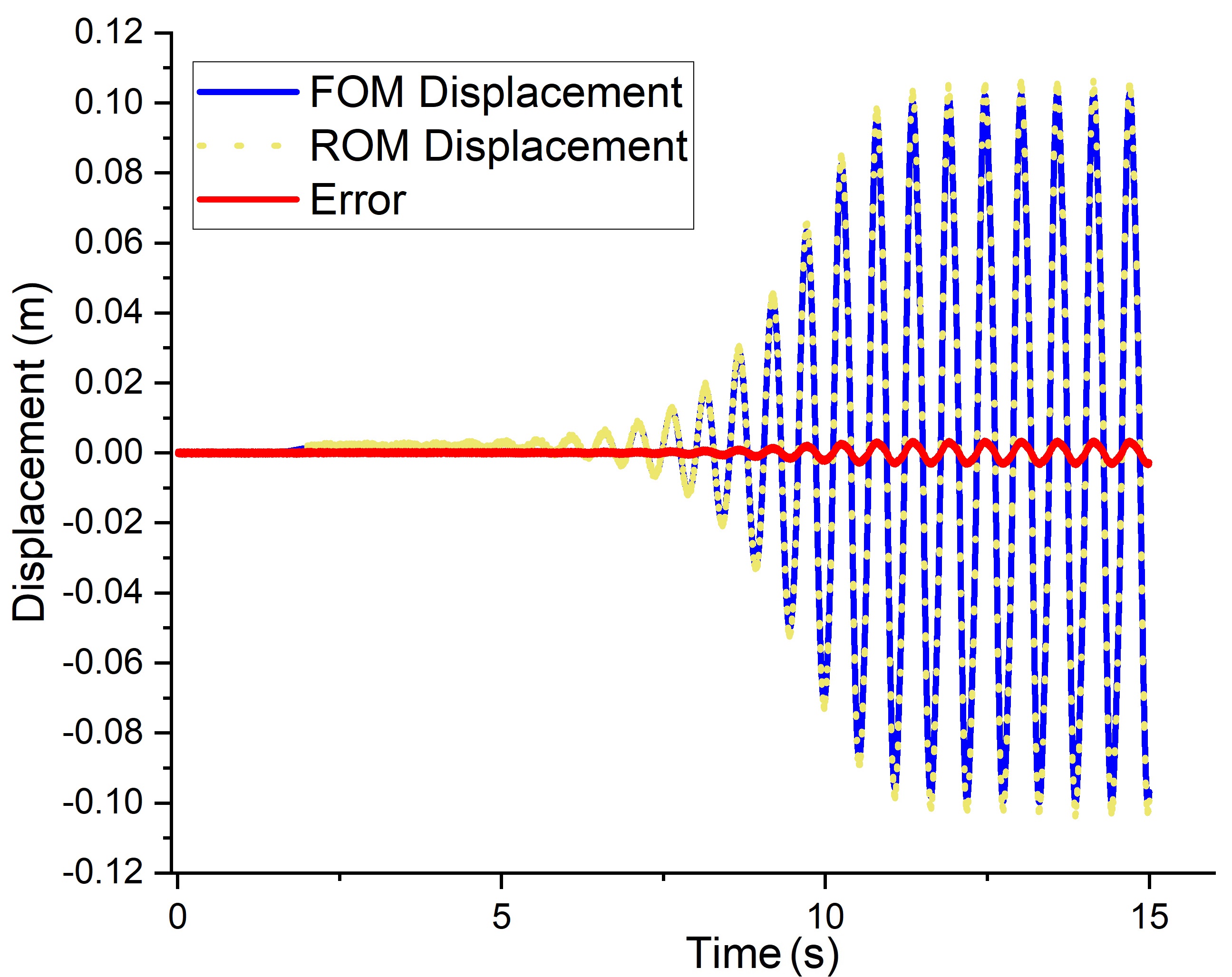
Figure 20: Error of $y$-displacement at point $A$ between FOM and ROM for Case $\mu_{s}=0.48\times 10^{6}$.

(a) Horizontal velocity of FOM

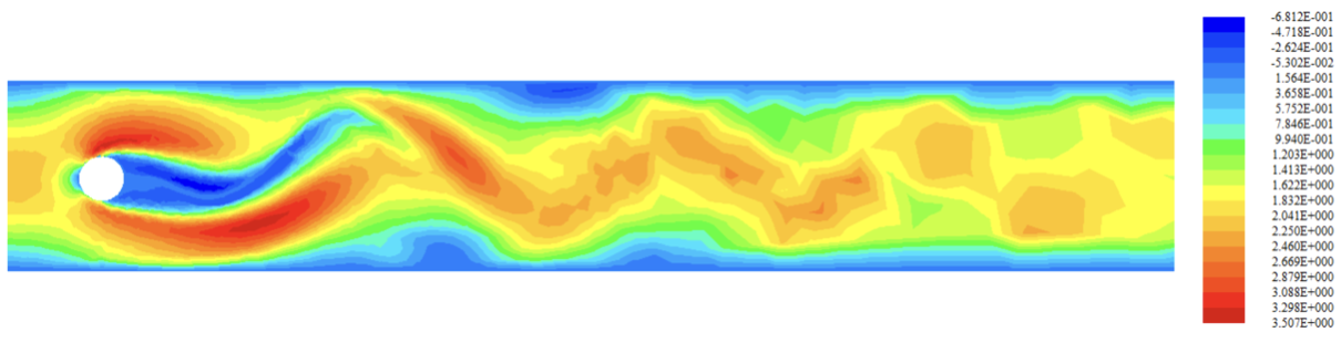
(b) Horizontal velocity of ROM

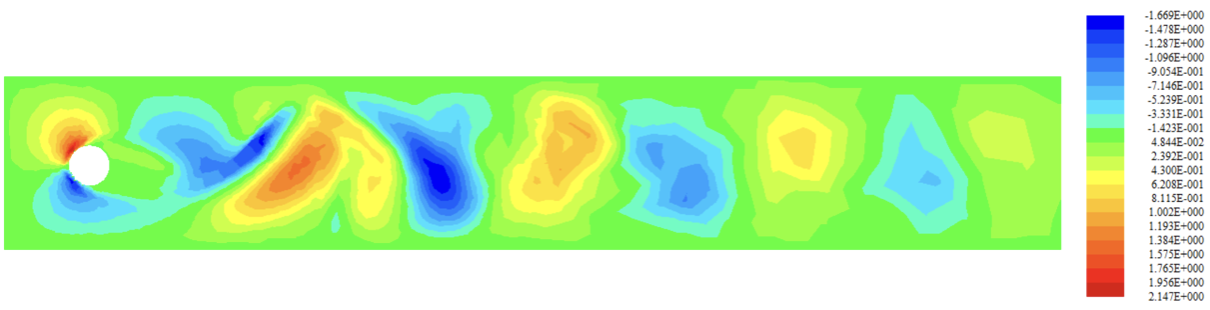
(c) Vertical velocity of FOM

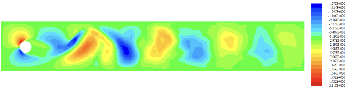
(d) Vertical velocity of ROM

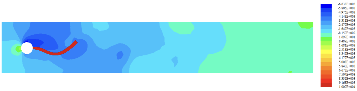
(e) Fluid pressure of FOM

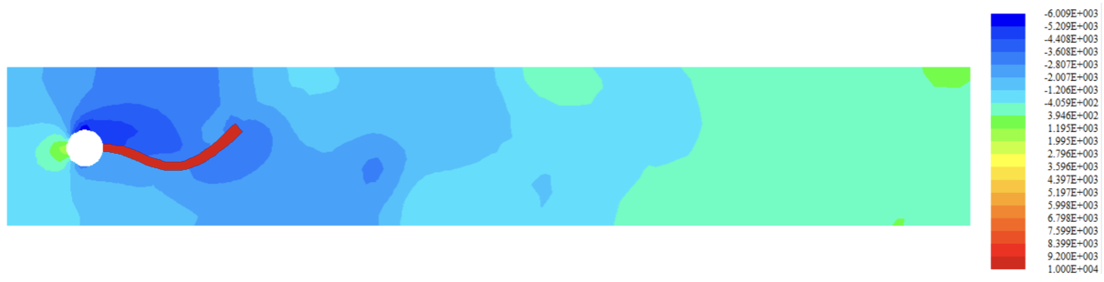
(f) Fluid pressure of ROM

Figure 21: FSI solutions between FOM and ROM at the finial time $t=15s$ for Case $\mu_{s}=0.48\times 10^{6}$.

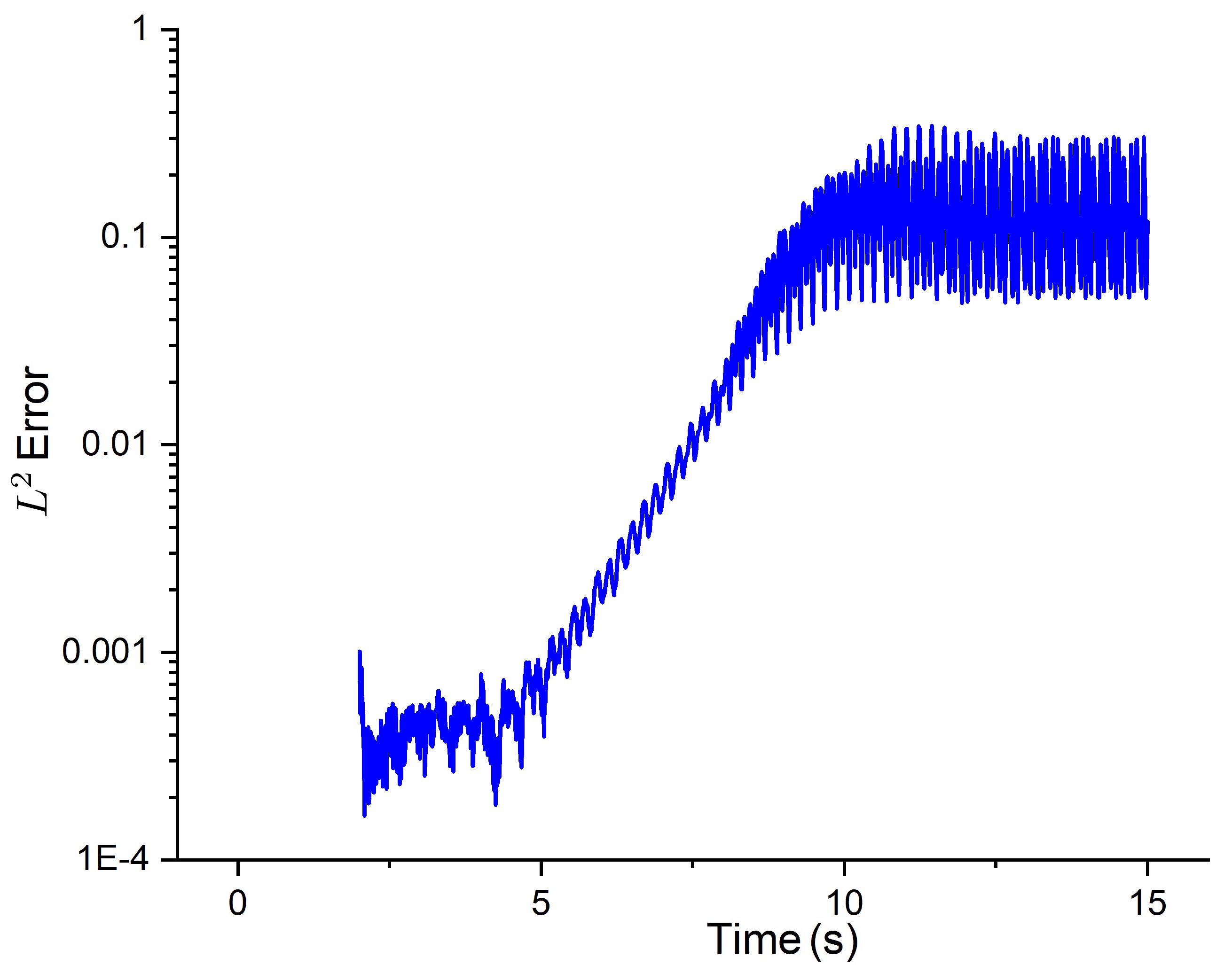
(a) Total error.

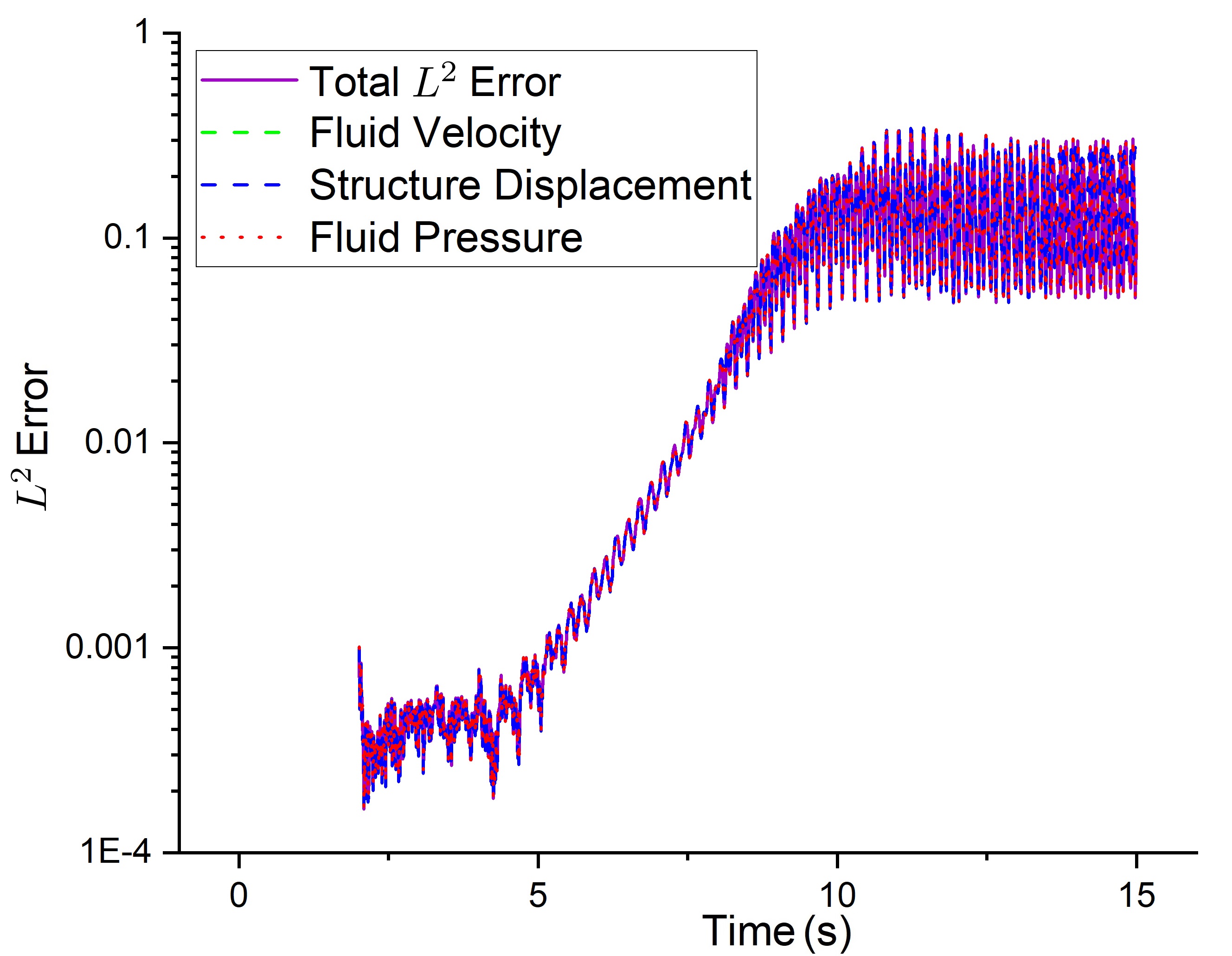
(b) Errors of all individual variables combining with total error.

Figure 22: Relative spatial $L^{2}$ errors between ROM and FOM over the entire time interval for Case $\mu_{s}=0.48\times 10^{6}$.

4.2 Motivation of partitioning the spatial and temporal dimension

As algorithmically discussed in Section 3 and numerically illustrated in Section 4.1, our developed ROM approach involves partitioning both the spatial and temporal dimensions, which has not yet been seen in the existing classical ROM for time-dependent problems including FSI. In this subsection, we illustrate why such a detailed partition of spatial and temporal dimensions is necessary by comparing results of the FOM and the classical ROM for the presented benchmark problem on a coarse mesh and time partition: 4751 DOFs in total and $\Delta t=0.01s$, while keeping all the other parameters unchanged.

First of all, we investigate the case of no partition for any spatial and temporal dimensions, which means $G=1$ then $g=0$, only, thus there is only one time segment: $[T_{0},T_{1}]=[2s,15s]$, leading to $N_{T_{0}}=1301$, as well as $\mathcal{N}_{h}=4751$. Therefore, the correlation matrices (19) turns out to be ${\mathcal{C}}_{\bm{U}_{0}}:={\bm{U}_{0}}^{\top}\bm{U}_{0}$ that belongs to $\mathbb{R}^{{N_{T_{0}}}\times{N_{T_{0}}}}$. As (20) shows, we calculate all eigenvalues and corresponding eigenvectors, then select sufficiently enough POD bases and perform the online phase.

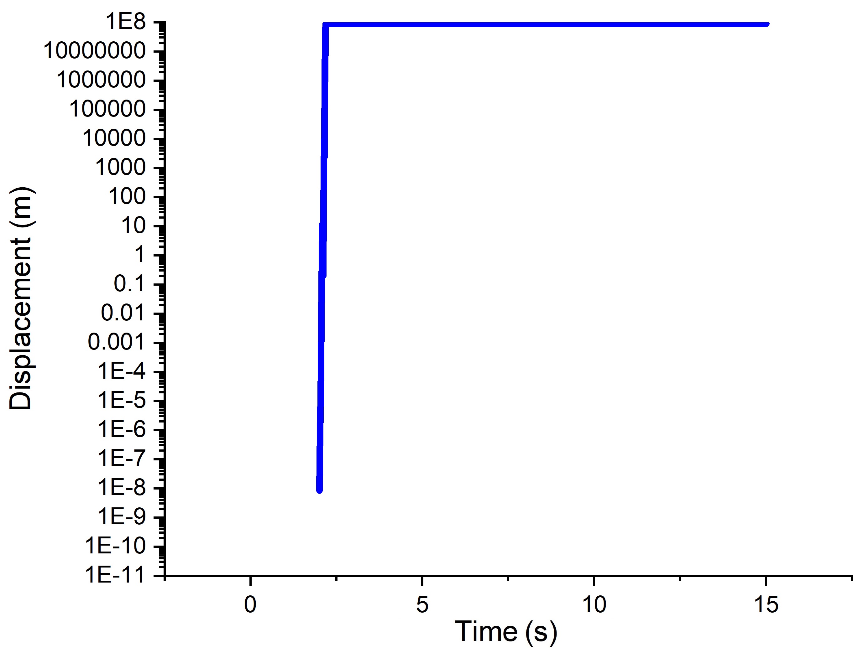
(a) Vibration curve at point $A$

(b) Total relative spatial $L^{2}$ error

Figure 23: ROM results without partition for spatial and temporal dimensions.

The obtained ROM results are shown in Figure 23, where we can see that right after the ROM computation starts, the total relative spatial $L^{2}$ error increases rapidly as high as $10^{12}$, correspondingly, the vibration amplitude of point $A$ also increases rapidly to the value around $10^{8}$, which far deviates from the FOM result, showing that such designed ROM completely fails in this FSI problem.

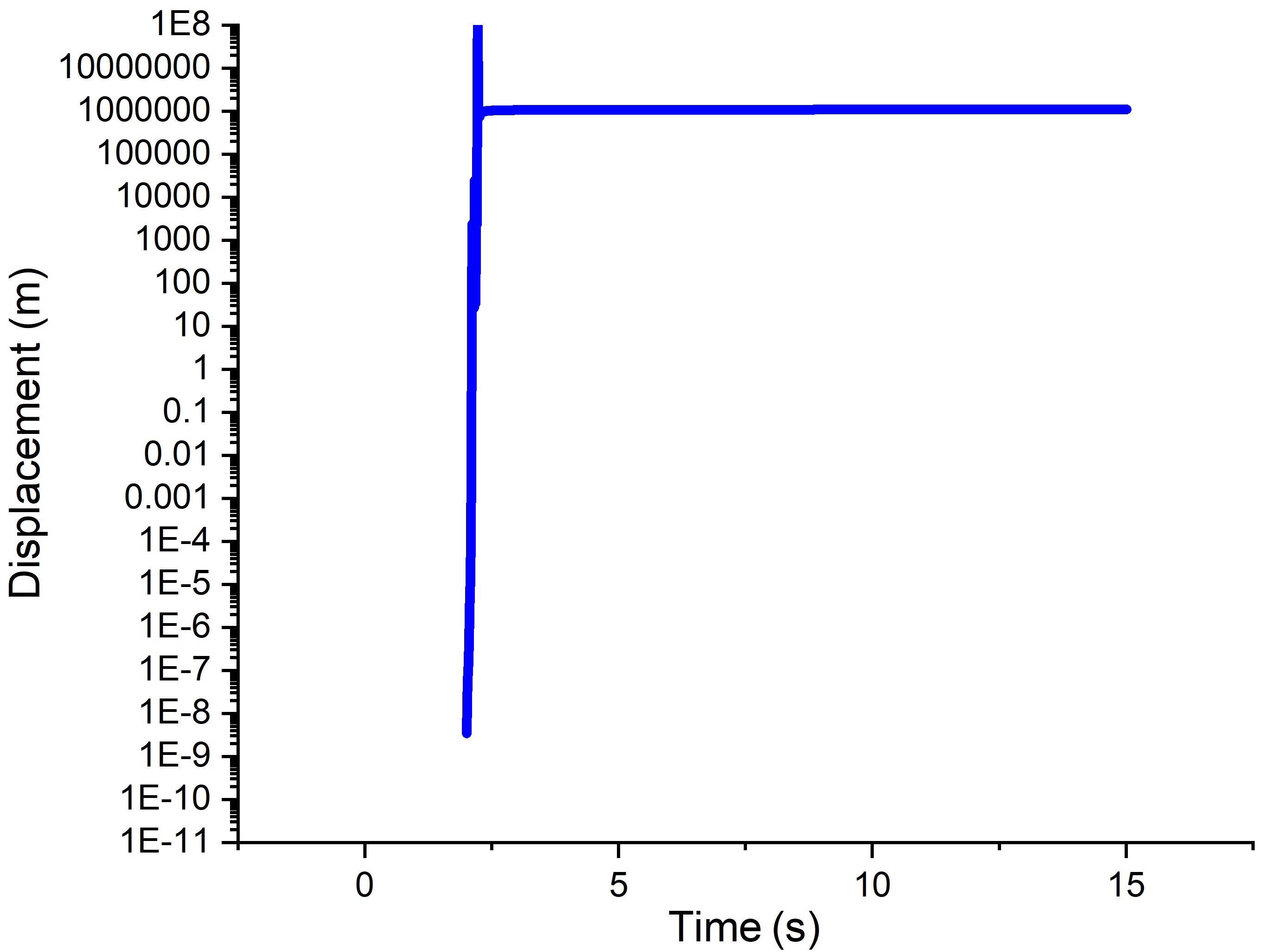
(a) Vibration curve at point $A$

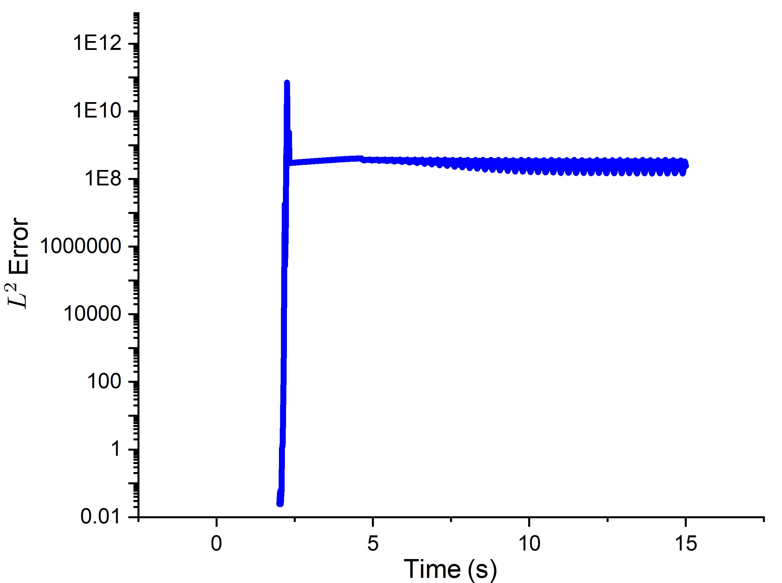
(b) Total relative spatial $L^{2}$ error

Figure 24: ROM results without a partition of temporal dimension.

In the second case, we only partition spatial dimensions in the same way as described in Section 3.1 but no partition for the temporal dimension, i.e., we still keep $G=1$ and $N_{T_{0}}=1301$. Then we select sufficiently enough POD bases in the online phase, and perform the ROM computation whose results are shown in Figure 24. We can observe that although the total relative spatial $L^{2}$ error decreases one magnitude in comparison with Figure 23, it is still as large as $10^{11}$. In addition, the vibration curve of point $A$ also deviates quickly from the FOM result, jumps to $10^{8}$ or so in a short time, resulting in a failure again.

However, if we partition both spatial and temporal dimensions, then just like what we do in Section 4.1, we can obtain a good match for the vibration curve of point $A$ between the ROM and FOM on this coarse mesh and time partition, where the ROM result holds a comparable accuracy to the FOM in terms of both spatial- and spatio-temporal $L^{2}$ errors, relatively. Therefore, we conclude that partitioning both spatial and temporal dimensions is greatly important and crucial for FSI problems when the structure significantly deforms with time.

5 Conclusion

In this work, we develop a novel reduced order model (ROM) approach to solve fluid-structure interaction (FSI) problems in an efficient fashion while the accuracy is still within a reasonable range in comparison with the solution of full-order model (FOM) approach. The key innovation is to treat time as a non-reduced variable while dividing the time interval into some time segments, and within each time segment we utilize the classical proper orthogonal decomposition (POD) method to achieve the order reduction in the offline phase. By selectively combining the time-segmented POD models, we apply the proposed ROM approach to a FSI benchmark problem and solve the issue of increasing error on the beam tail’s vibration amplitude over long-term simulations in the online phase. This hybrid strategy maintains the approximation accuracy for predicting the beam tail’s vibration under the circumstance of what the FOM requires, while speeding up the linear algebraic solver 8800 times more and saving the computational time for almost $100\%$ corresponding to the FOM, simultaneously, retaining the generalizability of offline model when physical parameters are perturbed for the entire system in the online application. Our approach demonstrates both the computational efficiency and the robustness for parameters’ perturbation, and overcomes limitations of standard POD reductions for FSI problems with long transient responses while the structure significantly deforms with time.

6 Acknowledgement

Q. Zhai and X. Xie were partially supported by the National Natural Science Foundation of China (12171340), S. Zhang was supported by Natural Science Foundation of Sichuan Province, China (2023NSFSC0075), and P. Sun was supported in part by a grant from the Simons Foundation (MPS-706640).

References

- [1] J. S. Anttonen, P. I. King, and P. S. Beran, POD-based reduced-order models with deforming grids, Mathematical and Computer Modelling, 38 (2003), pp. 41–62.
- [2] M. Astorino, F. Chouly, and M. A. Fernández, Robin based semi-implicit coupling in fluid-structure interaction: Stability analysis and numerics, SIAM Journal on Scientific Computing, 31 (2010), pp. 4041–4065.
- [3] F. Ballarin and G. Rozza, POD-Galerkin monolithic reduced order models for parametrized fluid-structure interaction problems, International Journal for Numerical Methods in Fluids, 82 (2016), pp. 1010–1034.
- [4] F. Ballarin, G. Rozza, and Y. Maday, Reduced-order semi-implicit schemes for fluid-structure interaction problems, Model Reduction of Parametrized Systems, (2017), pp. 149–167.
- [5] A. Barker and X. Cai, NKS for fully coupled fluid-structure interaction with application, in Domain Decomposition Methods in Science and Engineering XVIII, Springer, 2009, pp. 275–282.
- [6] P. S. Beran, D. J. Lucia, and C. L. Pettit, Reduced-order modelling of limit-cycle oscillation for aeroelastic systems, Journal of Fluids and Structures, 19 (2004), pp. 575–590.
- [7] M. Bergmann, A. Ferrero, A. Iollo, E. Lombardi, A. Scardigli, and H. Telib, A zonal Galerkin-free POD model for incompressible flows, Journal of Computational Physics, 352 (2018), pp. 301–325.
- [8] R. Bourguet, M. Braza, and A. Dervieux, Reduced-order modeling of transonic flows around an airfoil submitted to small deformations, Journal of Computational Physics, 230 (2011), pp. 159–184.
- [9] P. Causin, J. Gerbeau, and F. Nobile, Added-mass effect in the design of partitioned algorithms for fluid–structure problems, Computer methods in applied mechanics and engineering, 194 (2005), pp. 4506–4527.
- [10] H. Cho, Efficient semi-implicit coupling fluid-structure interaction analysis via model-order reduction of dynamic grids, Aerospace Science and Technology, 121 (2022), p. 107356.
- [11] A. de Castro, P. Kuberry, I. Tezaur, and P. Bochev, A novel partitioned approach for reduced order model – finite element model (ROM-FEM) and ROM-ROM coupling, arXiv:2206.04736, (2022).
- [12] L. Gastaldi, A priori error estimates for the arbitrary Lagrangian Eulerian formulation with finite elements, East-West J. Numer. Math., 9 (2001), pp. 123–156.
- [13] C. Grandmont, V. Guimet, and Y. Maday, Numerical analysis of some decoupling techniques for the approximation of the unsteady fluid-structure interaction., Mathematical Models and Methods in Applied Sciences, 11 (2001), pp. 1349–1377.
- [14] W. Hao, P. Sun, J. Xu, and L. Zhang, Multiscale and monolithiic arbitrary Lagrangian-Eulerian finite element method for a hemodynamic fluid-structure interaction problem involving aneurysms, Journal of Computational Physics, 433 (2021), p. 110181.
- [15] K. C. Hoang, Y. Choi, and K. Carlberg, Domain-decomposition least-squares Petrov-Galerkin (DD-LSPG) nonlinear model reduction, Computer Methods in Applied Mechanics and Engineering, 384 (2021), pp. 113997–113997.
- [16] G. Hou, J. Wang, and A. Layton, Numerical Methods for Fluid-Structure Interaction - A Review, Communications in Computational Physics, 12 (2012), pp. 337–377.
- [17] A. Huerta and W. Liu, Viscous flow structure interaction, Trans. ASME J. Pressure Vessel Technol., 110 (1988), pp. 15–21.
- [18] T. Hughes, L. Franca, and M. Balestra, A new finite element formulation for computational fluid dynamics: V. circumventing the Babuska-Brezzi condition: a stable Petrov-Galerkin formulation of the Stokes problem accommodating equal-order interpolations, Comput. Meth. Appl. Mech. Engrg., 59 (1986), pp. 85 – 99.
- [19] T. Hughes, W. Liu, and T. Zimmermann, Lagrangian-Eulerian finite element formulation for incompressible viscous flows, Comput. Methods Appl. Mech. Eng., 29 (1981), pp. 329–349.
- [20] S. Idelsohn, P. Del, R. Rossi, and E. O. nate, Fluid-structure interaction problems with strong added-mass effect, Int. J. Numer. Methods Eng., 80 (2009), pp. 1261–1294.
- [21] I. Kalashnikova, M. Barone, and M. Brake, A stable Galerkin reduced order model for coupled fluid–structure interaction problems, International Journal for Numerical Methods in Engineering, 95 (2013), pp. 121–144.
- [22] R. Lan and P. Sun, A novel arbitrary Lagrangian-Eulerian finite element method for a mixed parabolic problem on a moving domain, Journal of Scientific Computing, 85 (2020), p. 9.
- [23] , A novel arbitrary Lagrangian-Eulerian finite element method for a parabolic/mixed parabolic moving interface problem, Journal of Computational and Applied Mathematics, 383 (2021), p. 113125.
- [24] U. Langer and H. Yang, Robust and efficient monolithic fluid-structure-interaction solvers, International Journal for Numerical Methods in Engineering, 108 (2016), pp. 303–325.
- [25] R. LeVeque and Z. Li, The immersed interface method for elliptic equations with discontinuous coefficients and singular sources, SIAM J. Numer. Anal., 31 (1994), pp. 1019–1044.
- [26] J. Li, T. Zhang, S. Sun, and B. Yu, Numerical investigation of the pod reduced-order model for fast predictions of two-phase flows in porous media, International Journal of Numerical Methods for Heat & Fluid Flow, 29 (2019), pp. 4167–4204.
- [27] Z. Li and M.-C. Lai, The immersed interface method for the Navier-Stokes equations with singular forces, J. Comput. Phys., 171 (2001), pp. 822–842.
- [28] C. Nitikitpaiboon and K. Bathe, An arbitrary Lagrangian-Eulerian velocity potential formulation for fluid-structure interaction, Comput. Struct., 47 (1993), pp. 871–891.
- [29] F. Nobile and L. Formaggia, A Stability Analysis for the Arbitrary Lagrangian Eulerian Formulation with Finite Elements, East-West Journal of Numerical Mathematics, 7 (2010), pp. 105–132.
- [30] M. Nonino, F. Ballarin, G. Rozza, and Y. Maday, Overcoming slowly decaying kolmogorov n-width by transport maps: application to model order reduction of fluid dynamics and fluid–structure interaction problems, arXiv:1911.06598, (2019).
- [31] M. Nonino, F. Ballarin, G. Rozza, and Y. Maday, Projection based semi-implicit partitioned reduced basis method for fluid-structure interaction problems, Journal of Scientific Computing, 94 (2022).
- [32] C. Peskin, Flow patterns around heart valves: a numerical method, J. Comput. Phys., 10 (1972), pp. 252–271.
- [33] , The immersed boundary method, Acta Numer., 11 (2002), pp. 479–517.
- [34] A. Quarteroni and G. Rozza, Reduced Order Methods for Modeling and Computational Reduction, Springer, 06 2014.
- [35] T. Richter, Fluid-structure interactions, vol. 118 of Lecture Notes in Computational Science and Engineering, Springer International Publishing, 2017.
- [36] G. Rozza, Reduced basis methods for stokes equations in domains with non-affine parameter dependence, Computing and Visualization in Science, 12 (2006), pp. 23–35.
- [37] P. B. Ryzhakov, R. Rossi, S. R. Idelsohn, and E. Oñate, A monolithic Lagrangian approach for fluid-structure interaction problems, Computational Mechanics, 46 (2010), pp. 883–899.
- [38] G. Sieber, Numerical Simulation of Fluid-Structure Interaction Using Loose Coupling Methods, PhD thesis, TU Darmstadt, September 2002.
- [39] M. Souli and D. J. Benson, eds., Arbitrary Lagrangian Eulerian and Fluid-Structure Interaction: Numerical Simulation, Wiley-ISTE, 2010.
- [40] A. Tello Guerra, Fluid structure interaction using reduced order modeling: a first approach, Master’s thesis, Universitat Politècnica de Catalunya, 2014.
- [41] T. Tezduyar, Stabilized finite element formulations for incompressible flow computations, Adv. Appl. Mech., 28 (1992), pp. 1 – 44.
- [42] S. Turek and J. Hron, Proposal for numerical benchmarking of fluid-structure interaction between an elastic object and laminar incompressible flow, Springer, 2006.
- [43] S. Turek, J. Hron, M. Razzaq, H. Wobker, and M. Schäfer, Numerical benchmarking of fluid-structure interaction: A comparison of different discretization and solution approaches, Springer, 2010.
- [44] J. Vierendeels, L. Lanoye, J. Degroote, and P. Verdonck, Implicit coupling of partitioned fluid–structure interaction problems with reduced order models, Computers & structures, 85 (2007), pp. 970–976.
- [45] W. Wang, Y. Yan, L. Zhang, and C. Zhang, A monolithic fluid-structure interaction approach based on the pressure Poisson equation, Engineering Mechanics, 29 (2012), pp. 9–15.
- [46] H. Yang, C. Yang, and S. Sun, Active-set reduced-space methods with nonlinear elimination for two-phase flow problems in porous media, SIAM Journal on Scientific Computing, 38 (2016), pp. B593–B618.
- [47] K. Yang, P. Sun, L. Wang, J. Xu, and L. Zhang, Modeling and simulation for fluid-rotating structure interaction, Comput. Methods Appl. Mech. Engrg., 311 (2016), pp. 788–814.
- [48] Q. Zhai, Q. Hong, and X. Xie, A new reduced basis method for parabolic equations based on single-eigenvalue acceleration, Adv. Appl. Math. Mech., 2024 (accepted).