Model Predictive Bang-Bang Controller Synthesis via Approximate Value Functions

Abstract

: In this paper, we propose a novel method for addressing Optimal Control Problems (OCPs) with input-affine dynamics and cost functions. This approach adopts a Model Predictive Control (MPC) strategy, wherein a controller is synthesized to handle an approximated OCP within a finite time horizon. Upon reaching this horizon, the controller is re-calibrated to tackle another approximation of the OCP, with the approximation updated based on the final state and time information. To tackle each OCP instance, all non-polynomial terms are Taylor-expanded about the current time and state and the resulting Hamilton-Jacobi-Bellman (HJB) PDE is solved via Sum-of-Squares (SOS) programming, providing us with an approximate polynomial value function that can be used to synthesize a bang-bang controller.

1 Introduction

A bang-bang controller exclusively operates at the extremities of admissible inputs, toggling between upper and lower bounds. This type of controller is used in numerous physical systems with only binary actuation capabilities. Consider, for instance, a thermostat which can only alternate between “on” and “off” states. For more general systems where inputs are constrained to be within some rectangular set, bang-bang controllers are the optimal solution to a large class of Optimal Control Problems (OCPs) that have input affine dynamics and costs. Because of their optimality, Bang-bang controllers are ubiquitous in a wide domain of applications from medicine (Ledzewicz and Schättler, 2002), semiconductor gas discharge (Kim et al., 2001), spacecraft maneuvers (Taheri and Junkins, 2018), etc. Over the years many methods to synthesize bang-bang controllers have been proposed including Jacobson et al. (1970); Dadebo et al. (1998); Kaya et al. (2004)

Numerical methods for solving OCPs can be broken down into two distinct categories, direct methods and indirect methods. Direct methods parameterize the system state and control trajectories by a finite sum of basis functions on a time discretisation mesh to convert the continuous-time infinite-dimensional OCP into a Nonlinear Programming (NLP) problem that can be solved numerically. There are many toolboxes using the direct approach including ICLOCS (Nie et al., 2018) and GPOPs (Patterson and Rao, 2014), with the subsequent NLPs solved using solvers such as SNOPT (Gill et al., 2005) and IPOPT (Biegler and Zavala, 2009). Direct methods have demonstrated impressive capabilities. However, as noted in Aghaee and Hager (2021), when it comes to OCPs that have bang-bang solutions direct methods may struggle due to “ill conditioning and discontinuities in the optimal control at the switching points”. Such computational issues of direct methods are also discussed in Pager and Rao (2022). Another obstacle associated with the direct method lies in the difficulty of finding the global optimal solution for the resulting NLP. Mitigating the risk of converging to local minima entails initializing the algorithm with a good initial guess at the solution, also known as warm starting.

Indirect methods for solving OCPs can be further broken down into two sub-categorizes, those based on Pontryagin Maximum Principle (PMP) and those based on Dynamic Programming (DP). The PMP provides necessary conditions for the optimality of an open-loop controller while DP is able to provide necessary and sufficient conditions for the optimality of a closed-loop controller through the Hamilton Jacobi Bellman (HJB) PDE. A more detailed discussion of the methods can be found in Liberzon (2011). The PMP method involves minimizing the Hamiltonian along the solution map of the adjoint equation. If the Hamiltonian is convex (implying a unique optimal controller), it has been shown in Preininger and Vuong (2018) that bang-bang controllers can be synthesized using the PMP. However, in general, this assumption is restrictive.

For these reasons, we focus on the DP approach to solving the optimal control problem. The disadvantage of using DP in continuous time, of course, is that it requires us to solve the HJB PDE – a notoriously difficult nonlinear PDE. Various methods for approximately solving the HJB PDE exist such as Kalise and Kunisch (2018) or Garcke and Kröner (2017). These methods typically require some sort of discretization of state and time. Alternatively, it is possible to approximately solve the HJB PDE by relaxing the equation to an inequality and applying the moment method (Zhao et al., 2017; Korda et al., 2016; Kamoutsi et al., 2017), Sum-of-Squares (SOS) programming (Ichihara, 2009; Jennawasin et al., 2011) or other approximation schemes (Sassano and Astolfi, 2012). The advantage of these HJB relaxation approaches is that you can certify properties of the resulting approximate solution to the HJB PDE, such as being a uniformly lower bound. For this reason, we adopt the Sum-of-Squares (SOS) approach to computing HJB sub-value functions as described in Jones and Peet (2020). This approach yields an approximate polynomial value function. A key advantage of this method is that by increasing the degree of the SOS problem, this function can be made arbitrary close (under the $L^{1}$-norm) to the true solution of the HJB PDE.

Unfortunately the work of Jones and Peet (2020) requires the vector field to be polynomial, which is not true for many applications. The contribution of this work, then, is to extend Jones and Peet (2020) to tackle non-polynomial OCPs. Specifically, We propose to Taylor expand non-polynomial terms and solve the resulting approximate OCP. Unfortunately, of course, accuracy of the Taylor expansion can only be guaranteed in a small neighborhood of the expansion point and degrades quickly as we move away from this point. To address this issue, we propose a Model Predictive Control (MPC) type framework where after a small time horizon, the Taylor expansion is re-computed and the controller is re-synthesized.
Notation: For $x\in\mathbb{R}^{n}$ we denote $||x||_{2}=\sqrt{\sum_{i=1}^{n}x_{i}^{2}}$. Let $C^{1}(\Omega,\Theta)$ be the set of continuous functions with domain $\Omega\subset\mathbb{R}^{n}$ and image $\Theta\subset\mathbb{R}^{m}$. We denote the space of polynomials $p:\mathbb{R}^{n}\to\mathbb{R}$ by $\mathbb{R}[x]$ and polynomials with degree at most $d\in\mathbb{N}$ by $\mathbb{R}_{d}[x]$. We say $p\in\mathbb{R}_{2d}[x]$ is Sum-of-Squares (SOS) if there exists $p_{i}\in\mathbb{R}_{d}[x]$ such that $p(x)=\sum_{i=1}^{k}(p_{i}(x))^{2}$. We denote $\sum_{SOS}^{d}$ to be the set of SOS polynomials of at most degree $d\in\mathbb{N}$ and the set of all SOS polynomials as $\sum_{SOS}$.

2 Solving OCPs Using Dynamic Programming

Consider the following nested family of Optimal Control Problems (OCPs), each initialized by $(x_{0},t_{0})\in\mathbb{R}^{n}\times[0,T]$,

$$V(x_{0},t_{0}):=\inf_{u,x}\int_{t_{0}}^{T}c(x(t),u(t),t)dt+g(x(T))$$

$$\text{ subject to, }\dot{x}(t)=f(x(t),u(t))\quad\text{ for all }t\in[t_{0},T],$$ (1)

$$(u(t),x(t))\in U\times\Omega\quad\text{ for all }t\in[t_{0},T],\quad x(t_{0})=x_{0},$$

where $c:\mathbb{R}^{n}\times\mathbb{R}^{m}\times\mathbb{R}\to\mathbb{R}$ is referred to as the running cost; $g:\mathbb{R}^{n}\to\mathbb{R}$ is the terminal cost; $f:\mathbb{R}^{n}\times\mathbb{R}^{m}\to\mathbb{R}^{n}$ is the vector field; $\Omega\subset\mathbb{R}^{n}$ is the state constraint, $U\subset\mathbb{R}^{m}$ is the input constraint set; and $T$ is the final time. For simplicity, throughout this paper, we assume the existence of unique solutions to the Ordinary Differential Equation (ODE) described by the nonlinear dynamics $\dot{x}=f(x(t),u(t))$, for every admissible input to the Optimal Control Problem (OCP) and initial condition $x_{0}\in\Omega$. This assumption is non-restrictive, as various well-established conditions ensure the existence and uniqueness of solution maps. For instance, when the vector field, $f$, is Lipschitz continuous, the solution map exists over a finite time interval. Moreover, this interval can be extended arbitrarily if the solution map remains within a compact set, as elaborated in Khalil (2002).

Solving OCPs is a formidable challenge due to their lack of analytical solutions. One approach to solve OCPs, often referred to as the Dynamic Programming (DP) method, reduces the problem to solving a nonlinear PDE. More specifically, rather than solving Opt. (1) we solve the following nonlinear PDE:

$$\nabla_{t}V(x,t)+\inf_{u\in U}\left\{c(x,u,t)+\nabla_{x}V(x,t)^{T}f(x,u)\right\}=0$$

$$\hskip 106.69783pt\text{ for all }(x,t)\in\mathbb{R}^{n}\times[t_{0},T]$$ (2)

$$V(x,T)=g(x)\quad\text{ for all }x\in\mathbb{R}^{n}.$$

Upon solving the HJB PDE (2) we can derive a controller as shown in the following theorem.

Theorem 1 (Liberzon (2011))

Consider the family of OCPs in Eq. (1) with $\Omega=\mathbb{R}^{n}$ (no state constraints). Suppose $V\in C^{1}(\mathbb{R}^{n}\times\mathbb{R},\mathbb{R})$ solves the HJB PDE (2). Then $u^{*}:[t_{0},T]\to U$ solves the OCP initialized at $(x_{0},t_{0})\in\mathbb{R}^{n}\times[0,T]$ if and only if

$$u^{*}(t)=k(\phi_{f}(x_{0},t,u^{*}),t)\text{ for all }t\in[t_{0},T],$$ (3)

$$\text{where }k(x,t)\in\arg\inf_{u\in U}\{c(x,u,t)+\nabla_{x}V(x,t)^{T}f(x,u)\}.$$ (4)

Note that Theorem 1 requires the solution to the HJB PDE to be differentiable. In practice this condition is often relaxed using a generalized notion of a solution to the HJB PDE, called a viscosity solution (Bardi et al., 1997). Also note that in the state unconstrained case, $\Omega=\mathbb{R}^{n}$, the solution to the HJB PDE corresponds to the optimal objective function of the OCP and is referred to as the value function.

Bang-Bang control: Given a solution to the HJB PDE (2), we can construct an optimal state feedback controller according to Eq. (4). However, Eq. (4) is an optimization problem in itself requiring us to compute the infimum over $u\in U$. Solving this optimization at every time-step during implementation could be impractical. Fortunately, for OCPs with input-affine dynamics and costs, this auxiliary optimization problem has an analytical solution.

Consider OCP (1), where the cost function is of the form $c(x,u,t)=c_{0}(x,t)+\sum_{i=1}^{m}c_{i}(x,t)u_{i}$, the dynamics are of the form $f(x,u)=f_{0}(x)+\sum_{i=1}^{m}f_{i}(x)u_{i}$, there are no state constraints, $\Omega=\mathbb{R}^{n}$, and the input constraints are of the form $U=[a_{1},b_{1}]\times...\times[a_{m},b_{m}]$. WLOG we assume $a_{i}=-1$ and $b_{i}=1$ for $i\in\{1,\dots,m\}$, that is $U=[-1,1]^{m}$, since we can always make the coordinate substitution $\tilde{u}_{i}=\frac{2u_{i}-2b_{i}}{b_{i}-a_{i}}$ for $i\in\{1,...,m\}$. Substituting this into Eq. (4) we obtain

$$k(x,t)\in\arg\inf_{u\in[-1,1]^{m}}\bigg{\{}\sum_{i=1}^{m}c_{i}(x,t)u_{i}+\nabla_{x}V(x,t)^{T}f_{i}(x)u_{i}\bigg{\}}.$$ (5)

The objective function in Eq. (5) is linear in the decision variables $u\in\mathbb{R}^{m}$, and since the constraints have the form $u_{i}\in[1,-1]$, it follows that Eq.  (5) can be analytically solved,

$$k_{i}(x,t)=-\operatorname{sign}(c_{i}(x,t)+\nabla_{x}V(x,t)^{T}f_{i}(x)).$$ (6)

3 Approximate Solutions of the HJB PDE

Let us view the problem of solving the HJB PDE (2) through the lens of optimization theory and consider this problem as a feasibility optimization problem with two equality constraints: the HJB PDE itself and the boundary condition. In optimization theory, when faced with a challenging non-convex problem, a common tactic is to relax the constraints of the optimization problem to make the feasible set convex. In the context of solving the HJB, the equality constraints make the feasible set non-convex. However, we may relax the equality constraints to inequality constraints in the following manner,

$$\text{Find }J\in C^{1}(\mathbb{R}^{n}\times\mathbb{R},\mathbb{R})\text{ subject to:}$$ (7)

$$\nabla_{t}J(x,t)+c(x,u,t)+\nabla_{x}J(x,t)^{T}f(x,u)\geq 0$$ (8)

$$\hskip 85.35826pt\text{for all }(x,u,t)\in\Omega\times U\times(t_{0},T),$$

$$J(x,T)\leq g(x)\text{ for all }x\in\Omega.$$ (9)

Now, if $V$ is a solution to the HJB PDE then it satisfies Eqs (8) and (9) since

$$0 =\nabla_{t}V(x,t)+\inf_{u\in U}\left\{c(x,u,t)+\nabla_{x}V(x,t)^{T}f(x,u)\right\}$$

$$\leq\nabla_{t}V(x,t)+c(x,u,t)+\nabla_{x}V(x,t)^{T}f(x,u)$$

$$\hskip 85.35826pt\text{for all }(x,u,t)\in\Omega\times U\times(t_{0},T).$$

Problem (7) is linear in the decision variable $J$. However, a function $J$, feasible for Problem (7), may be arbitrarily far from the value function. For instance, in the case $c(x,u,t)\geq 0$ and $0\leq g(x)<M$, the constant function $J(x,t)\equiv-C$ is feasible for any $C>M$. Thus, by selecting sufficiently large enough $C>M$, we can make $||J-V||$ arbitrary large, regardless of the chosen norm, $||\cdot||$. To address this issue, we propose a modification of Problem (7), wherein we include an objective of minimizing the $L^{1}$ distance to the true solution to the HJB PDE $\int_{\Lambda\times[t_{0},T]}|V(x,t)-J(x,t)|dxdt$, where $V$ is the unknown solution to the HJB PDE $\Lambda\subset\mathbb{R}^{n}$ is some compact set.

$$\inf_{J\in C^{1}(\mathbb{R}^{n}\times\mathbb{R},\mathbb{R})}\int_{\Lambda\times[t_{0},T]}|V(x,t)-J(x,t)|dxdt\text{ subject to:}$$ (10)

$$\nabla_{t}J(x,t)+c(x,u,t)+\nabla_{x}J(x,t)^{T}f(x,u)\geq 0$$

$$\hskip 85.35826pt\text{for all }(x,u,t)\in\Omega\times U\times(t_{0},T),$$

$$J(x,T)\leq g(x)\text{ for all }x\in\Omega.$$

Unfortunately, since $V$ is unknown we cannot simply solve Opt. (10). Fortunately, as we will see in the next proposition, feasible solutions to Problem (10) are “sub-value functions” – i.e. functions that uniformly lower bound the true value function. Then $\int_{\Lambda\times[t_{0},T]}|V(x,t)-J(x,t)|dxdt=\int_{\Lambda\times[t_{0},T]}V(x,t)dxdt-\int_{\Lambda\times[t_{0},T]}J(x,t)dxdt$ and since $\int_{\Lambda\times[t_{0},T]}V(x,t)dxdt$ is a constant it can be eliminated from the objective function.

Proposition 2

Suppose $J\in C^{1}(\mathbb{R}^{n}\times\mathbb{R},\mathbb{R})$ satisfies Eqs (8) and (9) and $\Omega$ is compact. Then

$$J(x,t)\leq V(x,t)\text{ for all }(x,t)\in\Omega\times[t_{0},T],$$

where $V$ is given by the objective function of the OCP (1).

Let $(x_{0},t_{0})\in\Omega\times[0,T]$. First suppose there is no feasible input to the OCP, then $V^{*}(x_{0},t_{0})=\infty$. Clearly in this case $J(x_{0},t_{0})<V^{*}(x_{0},t_{0})$ as $J$ is continuous and therefore is finite over the compact region ${\Omega}\times[0,T]$. Alternatively if there exists a feasible input, ${u}$, let us denote the resulting solution map of the underlying dynamics of the OCP by $\tilde{x}$, where $\tilde{x}(t)\in\Omega$ for all $t\in[t_{0},T]$ and $\tilde{x}(t_{0})=x_{0}$. By Eq. (8) we have $\text{for all }t\in[t_{0},T]$

$$\nabla_{t}J(\tilde{x}(t),t)+c(\tilde{x}(t),{\tilde{u}}(t),t)+\nabla_{x}J(\tilde{x}(t),t)^{T}f(\tilde{x}(t),{\tilde{u}}(t))\geq 0.$$

Now, using the chain rule we deduce

$$\frac{d}{dt}J(\tilde{x}(t),t)+c(\tilde{x}(t),{\tilde{u}}(t),t)\geq 0\text{ for all }t\in[t_{0},T].$$

Then, integrating over $t\in[t_{0},T]$, and since $J(\tilde{x}(T),T)\leq g(\tilde{x}(T))$ by Eq. (9), we have

$$J(x_{0},t_{0})\leq\int_{t_{0}}^{T} c(\tilde{x}(t),{\tilde{u}}(t),t)dt+g(\tilde{x}(T)).$$ (11)

Since Eq. (11) holds for any feasible input, we may take the infimum over all feasible inputs to show that $J(x_{0},t_{0})\leq V(x_{0},t_{0})$.

For the case that $c$, $g$ and $f$ are polynomials, $U=[-1,1]^{m}$ and $\Omega=\{x\in\mathbb{R}^{n}:R^{2}-||x||_{2}^{2}\geq 0\}$, and $h_{\Omega}$ are polynomials, we are now able to eliminate $V$ from Opt. (10) and tighten the optimization problem to the following Sum-of-Squares (SOS) optimization problem,

$$P_{d}\in\arg\max_{P\in\mathbb{R}_{d}[x]}c^{T}\alpha$$ (12)

$$\text{subject to: }k_{0},k_{1}\in\sum_{SOS}^{d},\quad s_{i}\in{\sum_{SOS}^{d}}\text{ for }i=0,1,\dots,m+2$$

$$P(x,t)=c^{T}Z_{d}(x,t),k_{0}(x)=g(x)-{P(x,T)}-s_{0}(x)(R^{2}-||x||_{2}^{2}),$$

$$k_{1}(x,u,t)=\nabla_{t}P(x,t)+c(x,u,t)+\nabla_{x}P(x,t)^{T}f(x,u)$$

$$\quad-s_{1}(x,u,t)(R^{2}-||x||_{2}^{2})-s_{2}(x,u,t)(t-t_{0})(T-t)$$

$$\quad-\sum_{i=1}^{m}s_{2+i}(x,u,t)(u_{i}+1)(1-u_{i}),$$

where $\alpha_{i}=\int_{\Lambda\times[t_{0},T]}Z_{d,i}(x,t)dxdt$ and $Z_{d}:\mathbb{R}^{n}\times\mathbb{R}\to\mathbb{R}^{\mathcal{N}_{d}}$ is the vector of monomials of degree $d\in\mathbb{N}$.

We next show that by solving Opt. (12) we can approximate value functions, solutions to the HJB PDE (2), to arbitrary accuracy with respect to the $L^{1}$ norm.

Proposition 3

Consider OCP (1), where $\Omega=\mathbb{R}^{n}$ (no state constraints), $c$, $g$ and $f$ are polynomials, $U=[-1,1]^{m}$ and $T>0$. If this OCP has a solution $(x^{*}(t),u^{*}(t))$ such that for some $R>0$ we have that

$$||x^{*}(t)||_{2}^{2}<R^{2}\text{ for all }t\in[0,T],$$ (13)

$$\text{ then }\lim_{d\to\infty}\int_{\Lambda\times[t_{0},T]}|V(x,t)-P_{d}(x,t)|dxdt=0,$$ (14)

where $V$ solves the HJB PDE (2) and $P_{d}$ is the solution to Opt. (12) for $d\in\mathbb{N}$.

The condition given in Eq. (13) ensures the value function of the state constrained ($\Omega=\{x\in\mathbb{R}^{n}:||x||_{2}<R\}$) and unconstrained versions ($\Omega=\mathbb{R}^{n}$) of the OCP are equivalent. Then, following the mollification arguments of Jones and Peet (2020) we approximation the Lipschitz continuous value function of the unconstrained OCP by a smooth function while satisfying the inequalities given Eqs (8) and (9). We then approximate this smooth function by a polynomial using the Weierstrass approximation theorem. We show using Putinar’s Positivstellensatz (Putinar, 1993) that this polynomial is feasible to Opt. (12). Hence, by optimality, the solution to Opt. (12) is closer to the value function under the $L^{1}$ than this feasible polynomial and this feasible polynomial can be made arbitrarily close to the value function, thus showing convergence.

4 MPC For Solving Non-Polynomial OCPs

We have seen that we can approximately solve the HJB PDE (2) by numerically solving Opt. (12) for OCPs with polynomial costs and dynamics. However, many practical problems are not polynomial, limiting the broader applicability of the method. To rectify this issue, faced with a non-polynomial OCP, we propose to first approximate the non-polynomial terms using a Taylor expansion about the initial condition of the OCP – i.e. $(x_{0},t_{0})$. More generally, we denote the Taylor operator as

$$\mathcal{T}_{y,d}f(x)$$ (15)

$$:=\sum_{k_{n}=0}^{d}\cdots\sum_{k_{1}=0}^{d}\frac{(x_{1}-y)^{k_{1}}}{k_{1}!}\cdots\frac{(x_{n}-y)^{k_{n}}}{k_{n}!}\left(\frac{\partial^{k_{1}+\dots k_{n}}f}{\partial x_{1}^{k_{1}}\dots\partial x_{n}^{k_{n}}}\right)(y).$$ (16)

Now, given an OCP (1), with input affine dynamics and cost, we denote the polynomial terms with a superscript “$p$” and non-polynomial terms with an “$np$” superscript as follows,

$$c(x,u,t) :=c_{0}^{p}(x,t)+\sum_{i=1}^{m}c_{i}^{p}(x,t)u_{i}+c_{0}^{np}(x,t)+\sum_{i=1}^{m}c_{i}^{np}(x,t)u_{i}.$$

$$g(x) :=g^{p}(x)+g^{np}(x).$$ (17)

$$f(x,u) :=f_{0}^{p}(x)+\sum_{i=1}^{m}f_{i}^{p}(x)u_{i}+f_{0}^{np}(x)+\sum_{i=1}^{m}f_{i}^{np}(x)u_{i}.$$

We then replace non-polynomial terms with their degree $k$ Taylor expansions about the initial state and time conditions of the OCP ($(x_{0},t_{0})$), that is replace $c_{i}^{np}(x,t)$ with $\mathcal{T}_{[x_{0},t_{0}],k}c_{i}^{np}(x,t)$ and similarly for terms $f^{np}_{i}$ and $g^{np}$. This yields an OCP parameterized exclusively by polynomials and which can be solved using the methods described in the preceding section – yielding a bang-bang feedback control law.

Unfortunately, of course, the resulting value function only matches the true value function near the initial conditions of the OCP, $(x_{0},t_{0})$. Because the feedback law is based on minimization of this value function, we expect that the performance of the resulting feedback controller will match the true optimal controller near the initial condition, but will diverge as the solution evolves. Therefore after implementing the controller over an implementation period of length $T_{I}>0$ we propose to re-synthesize the controller based on a new approximated OCP with non-polynomial terms expanded about a new initial condition $(x(t_{0}+T_{I}),t_{0}+T_{I})$ – yielding a new approximate value function and feedback law.

Finally, in order to reduce complexity of solving the SOS optimization problem, and inspired by the MPC framework, we take a receding horizon approach and only synthesize the controller over a reduced prediction horizon length $T_{h}\geq T_{I}$ (See Fig. 1). Of course, unless $T_{I}=T_{h}=T$, if the receding horizon solution is to match the solution to the original OCP, we must necessarily assume $T=\infty$ and in this case, we require $g(x)=0$ – i.e., there is no terminal cost. Note, however, that since we allow for time-varying dynamics and cost functions, we do not eliminate time as a dependent variable in the HJB or value function. Moreover, because these prediction horizons may be small we may wish to only approximate the value function over some reduced integration region that depends on the final state of the previous implementation period, that is $\Lambda=[\delta_{1}(x),\delta_{2}(x)]^{n}$ where $\delta_{i}:\mathbb{R}^{n}\to\mathbb{R}$. The resulting algorithm is illustrated in Fig. 1 and summarized in Algorithm 1.

Algorithm 1 Polynomial VF-based Bang-Bang MPC

Input:
OCP parameters: $c,f$ of Form (17), $T>0,x_{0}\in\mathbb{R}^{n}$
MPC parameters: $T_{h}>0$, $T_{I}>0$.
SOS parameters: $d\in\mathbb{N}$, $\delta_{1}$, $\delta_{2}$ $R>0$.
Taylor parameter: $k\in\mathbb{N}$.

1:for $t\in\{0,T_{I},2T_{I},\dots,T-T_{I}\}$ do

2:     $\tilde{c}(x,u,t)=c_{0}^{p}(x,t)+\sum_{i=1}^{m}c_{i}^{p}(x,t)u_{i}+\mathcal{T}_{[x_{0},t],k}c_{0}^{np}(x,t)+\sum_{i=1}^{m}\mathcal{T}_{[x_{0},t],k}c_{i}^{np}(x,t)u_{i}$ $\triangleright$ Replace running cost by Taylor approx cost

3:     $\tilde{f}(x,u)=f_{0}^{p}(x)+\sum_{i=1}^{m}f_{i}^{p}(x)u_{i}+\mathcal{T}_{x_{0},k}f_{0}^{np}(x)+\sum_{i=1}^{m}\mathcal{T}_{x_{0},k}f_{i}^{np}(x)u_{i}$ $\triangleright$ Replace dynamics by Taylor approx

4:     Compute $P_{d}$ by solving Opt. (12) for $\tilde{c},\tilde{f},R>0$ and $\tilde{g}(x)\equiv 0$ over $[t,t+T_{h}]$ with integration region $\Lambda=[\delta_{1}(x_{0}),\delta_{2}(x_{0})]^{n}$.

5:     $k_{i}(x,t)=-\operatorname{sign}(c_{i}(x,t)+\nabla_{x}P_{d}(x,t)^{T}f_{i}(x))$ $\triangleright$ Eq. (6)

6:     Simulate $\dot{x}^{*}(t)=f(x^{*}(t),k(x^{*}(t),t))$ over $t\in[t+T_{I}]$.

7:     $x_{0}=x^{*}(T_{I})$ $\triangleright$ Set initial condition to be terminal trajectory

8:end for

Figure 1: Figure illustrating that the error of the Taylor approximation in Alg. 1 grows with time, resetting after the implementation time, $T_{I}$, has passed. The controller is designed over a prediction horizon of length $T_{h}$, which could exceed the implementation time $T_{I}$.

5 Numerical Examples

We next present several numerical examples of using Algorithm 1 to solve OCPs. To evaluate the performance we approximate the objective/cost function over each implementation period using the Riemann sum:

$$\int_{0}^{T}c(\phi_{{f}}(x_{0},t, u),t)dt\approx\Delta t\sum_{i=1}^{T/T_{I}}\sum_{j=1}^{N-1}c(x_{i}(t),{u}_{i}(t_{i,j}),t_{i,j}),$$ (18)

where $(i-1)T_{I}=t_{i,1}<...<t_{i,N}=iT_{I}$, $\Delta t=t_{i,j+1}-t_{i,j}$ for all $i\in\{1,...,N-1\}$, ${u}_{i}$ is the controller synthesized for implementation over $[(i-1)T_{I},iT_{I}]$, and $x_{i}(t)$ can be found using Matlab’s ode45 function to solve $\dot{x}(t)=f(x(t),{u}_{i}(t))$.

All SOS programs are solved by utilizing Yalmip (Lofberg, 2004) in conjunction with the SDP solver Mosek (ApS, 2019). It’s worth noting that in every numerical example, we scale the dynamics to confine the state within the range of $[-1,1]^{n}$. This scaling strategy ensures that both the objective function and constraints of the associated SDP problem remain within relatively small values. Consequently, this prevents the SDP solver from terminating prematurely due to suspected unboundedness.

We benchmark Algorithm 1 against ICLOCS (Nie et al., 2018). Both methods are fundamentally different, being of the indirect and direct class of solution methods, but numerical examples demonstrate competitive performance. Furthermore, the receding horizon/MPC approach presented here may result in slower convergence rates. Additionally, both methods have multiple parameters that can be used to improve performance, so the results are not necessarily indicative of overall performance. Specifically, ICLOCS requires an initial solution guess whereas Algorithm 1 is based on solving a sequence of convex optimization problems and therefore requires no such initialization. Therefore, Algorithm 1 could be used to help warm start direct methods like ICLOCS.

Example 1 (Controlling the Van der Pol oscillator)

Consider the following OCP

$$\inf_{{u}}\bigg{\{}\int_{0}^{T}||x(t)-y_{ref}(t)||_{2}^{2}dt\bigg{\}}$$ (19)

$$\text{Subject to: }u(t)\in[-1,1],\quad x(0)=[0.75,0.75]^{\top}$$

$$\begin{bmatrix}\dot{x}_{1}(t)\\ \dot{x}_{2}(t)\end{bmatrix}=\begin{bmatrix}2x_{2}(t)\\ 10x_{2}(t)(0.21-1.2^{2}x_{1}(t))-0.8x_{1}(t)\end{bmatrix}+\begin{bmatrix}0\\ 1\end{bmatrix}u(t)$$

$$y_{ref}(t)=\begin{bmatrix}0.2\cos(-t)\\ 0.2\sin(-t)\end{bmatrix}.$$

The goal of OCP (19) is to minimize the tracking error between the state and some parametric clockwise circular curve of radius $0.2$. Although the dynamics of OCP (19) are polynomial the cost function is not.

The terminal time is set as $T=20$, controller implementation time is set to $T_{I}=0.5$ and prediction horizon is set to $T_{h}=1$. We use Alg. 1 to solve this OCP with the SOS program degree set to $d=5$, the Taylor expansion degree set to $k=4$, the integration region set to $\Lambda=[\delta_{1},\delta_{2}]^{n}$, where $\delta_{1}=-\delta_{2}=-0.75$, and the computation domain given by $R=||[0.75,0.75]^{\top}||_{2}$. Performance was analyzed using Eq. (18) with simulation time-step $\Delta t=0.01$ and a cost of $0.521206$ was found. In contrast, for the same $T_{I}$ and $T_{h}$, $51$ discretization points, and degree $3$ polynomial approximations of state trajectories and inputs, ICLOCS incurred a slightly larger cost of $0.560883$. Fig. 2(a) shows the phase space plot and the slight difference in the trajectories resulting from the two different methods. How the individual states vary with respect to time is given in Fig. 3 as we as a log plot of how the running cost, $||x(t)-y_{ref}(t)||_{2}^{2}$, varies with respect to time.

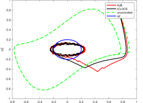
(a) Phase plot for Example 1.

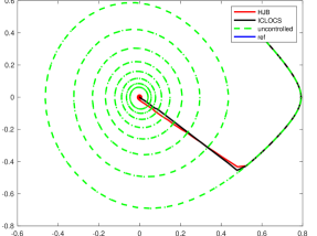
(b) Phase plot for Example 2.

Figure 2: Phase plots for Examples 1 and 2.

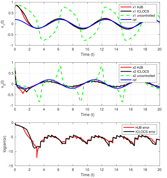
Figure 3: Figure associated with Example 1 showing how the controller effects individual states.

Example 2 (The Single Machine Infinite Bus (SMIB))

Improving the transient stability of the SMIB system has previously been studied in Chang and Chow (1998); Ford et al. (2006) using the PMP. We also solve this problem by considering the following OCP,

$$\inf_{{u}}\bigg{\{}\int_{0}^{T}e^{-t}||x(t)||_{2}^{2}dt\bigg{\}}$$ (20)

$$\text{Subject to: }u(t)\in[-1,1],\quad x(0)=[1.5,15]^{\top}$$

$$\begin{bmatrix}\dot{x}_{1}(t)\\ \dot{x}_{2}(t)\end{bmatrix}=\begin{bmatrix}x_{2}(t)\\ \frac{P_{m}-Dx_{2}(t)}{2H}\end{bmatrix}-\begin{bmatrix}0\\ \frac{P_{e}}{2H}\sin(x_{1}(t)+\delta_{ep})\end{bmatrix}u(t),$$

where $H=0.0106$, $X_{t}=0.28$, $P_{m}=1$, $E_{s}=1.21$, $V=1$, $P_{e}=(E_{s}V)/(P_{m}X_{t})$, $D=0.03$ and $\delta_{ep}=\sin^{-1}(1/P_{e})$.

Before solving the OCP we scale the dynamics to evolve over $[-1,1]^{2}$ by making the coordinate transformation $x\to Lx$ where $L=\begin{bmatrix}3&0\\ 0&30\end{bmatrix}$. The goal of this problem is to improve the transient stability – i.e. rate of convergence to the origin. Note that the problem has non-polynomial dynamics and cost.

The terminal time is set as $T=4$, controller implementation time is set to $T_{I}=0.25$ and prediction horizon is set to $T_{h}=0.5$. We use Alg. 1 to solve this OCP with the SOS program degree set to $d=6$, the Taylor expansion degree set to $k=5$, the integration region set to $\Lambda=[\delta_{1}(x),\delta_{2}(x)]^{n}$, where $\delta_{1}(x)=x-0.2$ and $\delta_{1}(x)=x+0.2$, and the computation domain given by $R=1$. Performance was analyzed using Eq. (18) with simulation time-step $\Delta t=0.01$ and a cost of $0.1672$ was found. In contrast, for the same $T_{I}$ and $T_{h}$, $51$ discretization points, and degree $3$ polynomial approximations of state trajectories and inputs, ICLOCS incurred a slightly smaller cost of $0.1671$. Fig. 2(b) shows the phase space plot and the slight difference in the trajectories resulting from the two different methods. How the individual states vary with respect to time is given in Fig. 4 as we as a log plot of how the running cost, $e^{-t}||x(t)||_{2}^{2}$, varies with respect to time.

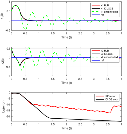
Figure 4: Figure associated with Example 2 showing how the controller effects individual states.

6 Conclusion

In this paper we have presented an iterative method for solving optimal control problems based on sequentially the approximated problem, whose dynamics and costs are Taylor expanded about the terminal state and time of the previous iteration. During each iteration, the HJB PDE is approximately solved using convex optimization and the resulting approximated value function is used to synthesize a bang-bang controller. Numerical examples demonstrate that this approach is competitive with the current state of the art direct method solver. Unlike direct methods, our method does not require an initial guess of the solution. Future work includes the possibility of precomputing a library of approximated value functions for different meshes of the state space and time interval offline. Then rather than sequentially solving the HJB PDE in an online MPC fashion the controller can be rapidly synthesized based on the current state and time by selecting the appropriate value function from this library.

References

- Aghaee and Hager (2021) Aghaee, M. and Hager, W.W. (2021). The switch point algorithm. SIAM Journal on Control and Optimization, 59(4), 2570–2593.
- ApS (2019) ApS, M. (2019). Mosek optimization toolbox for matlab. User’s Guide and Reference Manual, Version, 4, 1.
- Bardi et al. (1997) Bardi, M., Crandall, M.G., Evans, L.C., Soner, H.M., Souganidis, P.E., and Crandall, M.G. (1997). Viscosity solutions: a primer. Viscosity Solutions and Applications: Lectures given at the 2nd Session of the Centro Internazionale Matematico Estivo (CIME) held in Montecatini Terme, Italy, June 12–20, 1995, 1–43.
- Biegler and Zavala (2009) Biegler, L.T. and Zavala, V.M. (2009). Large-scale nonlinear programming using ipopt: An integrating framework for enterprise-wide dynamic optimization. Computers & Chemical Engineering, 33(3), 575–582.
- Chang and Chow (1998) Chang, J. and Chow, J. (1998). Time-optimal control of power systems requiring multiple switchings of series capacitors. IEEE transactions on power systems, 13(2), 367–373.
- Dadebo et al. (1998) Dadebo, S., McAuley, K., and McLellan, P. (1998). On the computation of optimal singular and bang–bang controls. Optimal Control Applications and Methods, 19(4), 287–297.
- Ford et al. (2006) Ford, J., Ledwich, G., and Dong, Z. (2006). Nonlinear control of single-machine-infinite-bus transient stability. In 2006 IEEE Power Engineering Society General Meeting, 8–pp. IEEE.
- Garcke and Kröner (2017) Garcke, J. and Kröner, A. (2017). Suboptimal feedback control of pdes by solving hjb equations on adaptive sparse grids. Journal of Scientific Computing, 70, 1–28.
- Gill et al. (2005) Gill, P.E., Murray, W., and Saunders, M.A. (2005). Snopt: An sqp algorithm for large-scale constrained optimization. SIAM review, 47(1), 99–131.
- Ichihara (2009) Ichihara, H. (2009). Optimal control for polynomial systems using matrix sum of squares relaxations. IEEE Transactions on Automatic Control, 54(5), 1048–1053.
- Jacobson et al. (1970) Jacobson, D., Gershwin, S., and Lele, M. (1970). Computation of optimal singular controls. IEEE Transactions on Automatic Control, 15(1), 67–73.
- Jennawasin et al. (2011) Jennawasin, T., Kawanishi, M., and Narikiyo, T. (2011). Performance bounds for optimal control of polynomial systems: A convex optimization approach. SICE Journal of Control, Measurement, and System Integration, 4(6), 423–429.
- Jones and Peet (2020) Jones, M. and Peet, M.M. (2020). Polynomial approximation of value functions and nonlinear controller design with performance bounds. arXiv preprint arXiv:2010.06828.
- Kalise and Kunisch (2018) Kalise, D. and Kunisch, K. (2018). Polynomial approximation of high-dimensional hamilton–jacobi–bellman equations and applications to feedback control of semilinear parabolic pdes. SIAM Journal on Scientific Computing, 40(2), A629–A652.
- Kamoutsi et al. (2017) Kamoutsi, A., Sutter, T., Esfahani, P.M., and Lygeros, J. (2017). On infinite linear programming and the moment approach to deterministic infinite horizon discounted optimal control problems. IEEE control systems letters, 1(1), 134–139.
- Kaya et al. (2004) Kaya, C.Y., Lucas, S.K., and Simakov, S.T. (2004). Computations for bang–bang constrained optimal control using a mathematical programming formulation. Optimal control applications and methods, 25(6), 295–308.
- Khalil (2002) Khalil, H. (2002). Nonlinear systems. 3rd edition.
- Kim et al. (2001) Kim, J.H., Maurer, H., Astrov, Y.A., Bode, M., and Purwins, H.G. (2001). High-speed switch-on of a semiconductor gas discharge image converter using optimal control methods. Journal of Computational Physics, 170(1), 395–414.
- Korda et al. (2016) Korda, M., Henrion, D., and Jones, C.N. (2016). Controller design and value function approximation for nonlinear dynamical systems. Automatica, 67, 54–66.
- Ledzewicz and Schättler (2002) Ledzewicz, U. and Schättler, H. (2002). Optimal bang-bang controls for a two-compartment model in cancer chemotherapy. Journal of optimization theory and applications, 114, 609–637.
- Liberzon (2011) Liberzon, D. (2011). Calculus of variations and optimal control theory: a concise introduction. Princeton university press.
- Lofberg (2004) Lofberg, J. (2004). Yalmip: A toolbox for modeling and optimization in matlab. In 2004 IEEE international conference on robotics and automation (IEEE Cat. No. 04CH37508), 284–289. IEEE.
- Nie et al. (2018) Nie, Y., Faqir, O., and Kerrigan, E.C. (2018). Iclocs2: Try this optimal control problem solver before you try the rest. In 2018 UKACC 12th international conference on control (CONTROL), 336–336. IEEE.
- Pager and Rao (2022) Pager, E.R. and Rao, A.V. (2022). Method for solving bang-bang and singular optimal control problems using adaptive radau collocation. Computational Optimization and Applications, 81(3), 857–887.
- Patterson and Rao (2014) Patterson, M.A. and Rao, A.V. (2014). Gpops-ii: A matlab software for solving multiple-phase optimal control problems using hp-adaptive gaussian quadrature collocation methods and sparse nonlinear programming. ACM Transactions on Mathematical Software (TOMS), 41(1), 1–37.
- Preininger and Vuong (2018) Preininger, J. and Vuong, P.T. (2018). On the convergence of the gradient projection method for convex optimal control problems with bang–bang solutions. Computational Optimization and Applications, 70, 221–238.
- Putinar (1993) Putinar, M. (1993). Positive polynomials on compact semi-algebraic sets. Indiana University Mathematics Journal, 42(3), 969–984.
- Sassano and Astolfi (2012) Sassano, M. and Astolfi, A. (2012). Dynamic approximate solutions of the hj inequality and of the hjb equation for input-affine nonlinear systems. IEEE Transactions on Automatic Control, 57(10), 2490–2503.
- Taheri and Junkins (2018) Taheri, E. and Junkins, J.L. (2018). Generic smoothing for optimal bang-off-bang spacecraft maneuvers. Journal of Guidance, Control, and Dynamics, 41(11), 2470–2475.
- Zhao et al. (2017) Zhao, P., Mohan, S., and Vasudevan, R. (2017). Control synthesis for nonlinear optimal control via convex relaxations. In 2017 American Control Conference (ACC), 2654–2661. IEEE.