Average-Case Analysis of Iterative Voting

Abstract

Iterative voting is a natural model of repeated strategic decision-making in social choice when agents have the opportunity to update their votes prior to finalizing the group decision. Prior work has analyzed the efficacy of iterative plurality on the welfare of the chosen outcome at equilibrium, relative to the truthful vote profile, via an adaptation of the price of anarchy. However, prior analyses have only studied the worst-case and average-case performances when agents’ preferences are distributed by the impartial culture. This work extends average-case analyses to a wider class of distributions and distinguishes when iterative plurality improves or degrades asymptotic welfare.

1 Introduction

It is well-known in social choice that people may misreport their preferences to improve group decisions in their favor. Consider, for example, Alice, Bob, and Charlie deciding on which ice cream flavor to order for a party, and Charlie prefers strawberry to chocolate to vanilla. Given that Alice wants chocolate and Bob wants vanilla, Charlie would be better off voting for chocolate than truthfully, in which vanilla may win by default. This form of strategic behavior is prolific in political science in narrowing the number of political parties (see e.g., Duvuger’s law (Riker, 1982)). Still, it is unclear what effect strategic behavior has on chosen outcomes.

Iterative voting (IV) is one model which naturally describes agents’ strategic behavior – in misreporting their truthful preferences – over time. After agents reveal their preferences initially, they have the opportunity to repeatedly update their votes given information about other agents’ votes, before the final decision is reached. Meir et al. (2010) first proposed iterative plurality voting and identified many sufficient conditions for IV to converge. This was followed up by a series of work examining various social choice rules, information and behavioral assumptions, and settings to determine when, to what outcomes, and how fast IV converges (see e.g. surveys by Meir (2017) and Meir (2018)).

While significant research has focused on the convergence and equilibrium properties of IV, only a few papers have analyzed its performance (Brânzei et al., 2013; Kavner and Xia, 2021). Given that strategic behavior is bound to occur (see the Gibbard-Satterthwaite theorem (Gibbard, 1973; Satterthwaite, 1975)), Brânzei et al. (2013) investigated how bad the resulting outcome could be. Brânzei et al. (2013) defined the dynamic price of anarchy (DPOA) as the ratio of social welfare between the truthful vote profile and the worst-case equilibrium that is reachable via IV. This notion is with respect to the worst-case preference profile and a given voting rule, and refines the well-known price of anarchy (Roughgarden and Tardos, 2002) for a dynamical setting with myopic agents. They found the performance is “very good” for plurality (with an additive-DPoA of $1$), “not bad” for veto (with a DPoA of $\Omega(m)$ with $m$ candidates, $m\geq 4$), and “very bad” for Borda (with a DPoA of $\Omega(n)$ with $n$ agents).

Notably, Brânzei et al. (2013)’s results assumed that the positional scoring rule had the same scoring vector as agents’ additive utilities. Kavner and Xia (2021) relaxed this assumption to arbitrary utility vectors with respect to iterative plurality. They found the additive DPoA worsened to $\Theta(n)$ in the worst-case. While this result bounds the theoretical consequences of IV, it provides little insight into how IV may perform realistically. Upon realizing this poor result, Kavner and Xia (2021) took a first step in testing IV’s practicality by exploring its average-case performance. By assuming that agents’ preferences are distributed identically and uniformly at random, known as the impartial culture (IC) distribution, they found the expected additive DPoA to be $-\Omega(1)$. This suggests that IV actually improves social welfare over the truthful vote profile on average.

Average-case analysis is traditionally employed in computer science as a way around the intractability of NP-hard problems. This analysis is motivated by the possibility that worst-case results only occur infrequently in practice (Bogdanov et al., 2006). As seen with IV, average-case analysis hopes to provide a less pessimistic measure of an algorithm’s performance. However, the distribution used in the analysis may itself be unrealistic (Spielman and Teng, 2009). Indeed, IC used by (Kavner and Xia, 2021) is widely understood to be an implausible distribution (see e.g., Tsetlin et al. (2003), Regenwetter (2006), and Van Deemen (2014)), yet useful perhaps as a benchmark against other analytical results in social choice. This presents an opportunity to advance our understanding of iterative plurality voting beyond IC.

1.1 Our Contribution

We address the limitations of the IC distribution by analyzing the average-case performance of IV with respect to a larger class of input preference distributions. Agent preferences are distributed independently and identically. Our primary result is a characterization of certain classes of preferences for which IV improve or degrades social welfare. We describe to what extent welfare changes as the number of agents increases, specified informally as follows.

Theorem 1 (Expected dynamic price of anarchy, informally put).

There are classes of i.i.d. preferences such that, for infinitely many agents $n\in\mathbbm{N}$, the expected performance of iterative plurality is $\Theta(1)$, $-\Theta(1)$, or $\pm\mathcal{O}\left(\frac{1}{\sqrt{n}}\right)$.

1.1.1 Technical innovations.

Our techniques begin similarly to Kavner and Xia (2021) in that we partition the expected performance of IV based on which set of alternatives are approximately-tied when agents vote truthfully and study each case separately. We further make use of a Bayesian network representation of agents’ preferences in order to effectively classify which group preference profiles by their economic performance and how likely each group is to occur. However, there are a number of places where Kavner and Xia (2021) proof breaks down. Namely, following their method directly would only yield a bound on IV’s expected performance of $\pm\mathcal{O}(\sqrt{n})$, which is insufficiently refined. Moreover, the preference distributions we study are slightly biased to increase the magnitude of IV’s performance, whereas IC in Kavner and Xia (2021)’s proof did not weight certain agents’ preference rankings more than others. These factors make our analysis significantly more complicated and require a collection of novel binomial and multinomial theorems to solve (see Appendices B – F).

Our analysis makes significant use of the PMV-in-Polyhedron theorem from Xia (2021a) to characterize the asymptotic likelihood of certain events. Specifically, we capture the likelihood that the histogram of a preference profile, which is a Poisson multivariate variable, fits into polyhedron that specify a tied election (Lemma 1 below) and with additional constraints (Lemma 5 below). Xia (2021a)’s techniques, and those in subsequent papers by Xia and colleagues, are not directly applicable in our setting because those paper characterize certain events occurring, whereas we study the expected performance of a protocol. Rather, we make novel use of their theorems in our present work.

1.2 Related Work

1.2.1 Iterative Voting

The present study of IV was initiated by Meir et al. (2010) who identified that iterative plurality converges when agents sequentially apply best-response updates. This inspired a line of research on sufficient conditions for convergence. Following (Meir et al., 2010), Lev and Rosenschein (2012) and Reyhani and Wilson (2012) simultaneously found that iterative veto converges while no other positional scoring rule does. Gourves et al. (2016) and Koolyk et al. (2017) followed up with similar negative results for other voting rules, such as Copeland and STV. In lieu of these negative results, Grandi et al. (2013), Obraztsova et al. (2015), and Rabinovich et al. (2015) proved convergence by imposing stricter assumptions on agents’ behavior, such as truth bias and voting with abstentions (Desmedt and Elkind, 2010; Thompson et al., 2013; Obraztsova et al., 2013; Elkind et al., 2015).

Reijngoud and Endriss (2012) and Endriss et al. (2016) take a different approach by relaxing assumptions about what information agents have access to. Rather than performing best-response updates, agents make local dominance improvement steps that may improve the outcome but cannot degrade the outcome, given their information (Conitzer et al., 2011). Meir et al. (2014) and Meir (2015) characterized convergence of iterative plurality with such local dominance improvements. Kavner et al. (2023) extended their model to settings where multiple issues are decided on simultaneously, similar to experiments by Bowman et al. (2014) and Grandi et al. (2022). Relatedly, Sina et al. (2015) and Tsang and Larson (2016) studied IV with agents embedded in social networks.

While most IV research focuses on convergence and equilibrium properties, Brânzei et al. (2013) quantified the quality of IV via the worst-case dynamic price of anarchy with respect to many voting rules. Kavner and Xia (2021) extended their results for iterative plurality with respect to any additive utility vector and in the average case, demonstrating an improvement in average social welfare despite poor worst-case performance. Meanwhile, other synthetic and human subjects experiments have proved inconclusive about the effects IV has on social welfare (Thompson et al., 2013; Bowman et al., 2014; Koolyk et al., 2017; Meir et al., 2020; Grandi et al., 2022). Our work provides a more comprehensive analysis of IV’s performance by extending the domain of agents’ input preference distributions. Other forms of sequential and IV include models by Airiau and Endriss (2009), Desmedt and Elkind (2010), and Xia and Conitzer (2010).

1.2.2 Smoothed Analysis

Spielman and Teng (2004) introduced smoothed analysis as a combination of worst- and average-case analyses to address the issue that average-case analysis distributions themselves may not be realistic. Their idea was to measure an algorithm’s performance with respect to a worst-case instance subject to a random perturbation. Hence, even if an algorithm has exponential worst-case complexity, we may be unlikely to encounter such an instance in practice. It has since been used in a large body of problems (see e.g., (Spielman and Teng, 2009; Roughgarden, 2021) for a survey). For example, Deng et al. (2022) studied the smoothed performance of the random priority mechanism in matching problems. Extensions into social choice were independently proposed by Baumeister et al. (2020) and Xia (2020). The latter inspired a series of research extending prior results through this lens (e.g., (Xia, 2021b; Xia and Zheng, 2021; Liu and Xia, 2022; Xia and Zheng, 2022; Xia, 2023) and references within). Notably, Xia (2021a) studied the smoothed likelihood of ties in elections, which contributes meaningfully toward our primary results. We describe in the discussion section how our work can be framed within this perspective advanced by Xia (2020).

2 Preliminaries

Basic setting.

Let $\mathcal{A}=\{1,\ldots,m\}$ denote the set of $m\geq 3$ alternatives and $n\in\mathbb{N}$ denote the number of agents. Unless stated otherwise, we assume that $m=3$ throughout this work. Each agent $j\leq n$ is endowed with a preference ranking $R_{j}\in\mathcal{L}(\mathcal{A})$, the set of strict linear orders over $\mathcal{A}$. A preference profile is denoted $P=(R_{1},\ldots,R_{n})$. For any pair of alternatives, $a,b\in\mathcal{A}$, we use $P[a\succ b]$ to denote the number of agents that prefer $a$ to $b$ in $P$.

Agents vote by reporting a single alternative $a_{j}\in\mathcal{A}~{}\forall j\leq n$. The collection of votes $a=(a_{1},\ldots,a_{n})$ is called a vote profile. A vote $a^{*}_{j}=\textit{top}(R_{j})$ is truthful if it agent $j$’s most-favored alternative. The score vector $\vec{s}(a)=(s_{c}(a))_{c\in\mathcal{A}}$ depicts the histogram of scores for each alternative, where $s_{c}(a)=|\{j\leq n:a_{j}=c\}|$. In this work we use the plurality rule: $\tilde{f}(a)=\operatorname*{arg\,max}_{c\in\mathcal{A}}s_{c}(a)$ is a set; $f(a)\in\tilde{f}(a)$ imposes lexicographical tie-breaking.

Rank-based additive utility.

We take agents with additive utilities characterized by a rank-based utility vector $\vec{u}:=(u_{1},\ldots,u_{m})\in\mathbb{R}^{m}_{\geq 0}$ with $u_{1}\geq\ldots u_{m}$ and $u_{1}>u_{m}$. For example, plurality welfare has $\vec{u}=(1,0,\ldots,0)$ while Borda welfare has $\vec{u}=(m-1,m-2,\ldots,0)$. Each agent $j$ gets $\vec{u}(R_{j},a)=u_{i}$ utility for the alternative $a\in\mathcal{A}$ ranked $i^{th}$ in $R_{j}$. The additive social welfare of $a$ according to preference profile $P$ is $\text{SW}_{\vec{u}}(P,a)=\sum_{j=1}^{n}\vec{u}(R_{j},a)$.

Iterative plurality voting.

Given an agent preference preferences $P$, we initialize the vote profile $a(0)=a^{*}$ as truthful. We then consider an iterative process of vote profile $a(t)=(a_{1}(t),\ldots,a_{n}(t))$ that describe agents’ reported votes over time $t\geq 0$. For each round $t$, a scheduler chooses an $j$ to improve their vote to the best response of all others (Apt and Simon, 2015). All other votes besides $j$’s remain unchanged. Vote profiles where no such improvement step exists are called (Nash) equilibrium. Let $\text{EW}(a(t))$ denote the unique set of alternatives that are plurality winners of any equilibrium reachable via best-response dynamics from the vote profile $a(t)$. We distinguish this from the set of potentially winning alternatives, $\text{PW}(a(t))$, which could be the winner with an additional vote on round $t$. It follows that $\text{PW}(a^{*})$ are alternatives that are approximately-tied in $a^{*}$.

2.1 Dynamic Price of Anarchy

The performance of IV is commonly measured by a worst-case comparison in social welfare between the truthful vote profile and the equilibrium that are reachable via the dynamics. This captures the impact that IV has against the outcome that would take place without agents’ strategic manipulation of their votes. Moreover, it does not assume that the order agents make their improvement steps is controlled; the measure is over the worst-case scheduler. In the following definitions, we consider this performance measure according to the worst-case preference profile $P$ as well as the average-case analysis when $P$ is sampled from some distribution $\pi_{n}$.

Definition 1 (Additive Dynamic Price of Anarchy (ADPoA) (Brânzei et al., 2013)).

Given $n\in\mathbb{N}$, a utility vector $\vec{u}$, and preferences $P$, the adversarial loss starting from the truthful vote profile $a^{*}$ is

$$\text{D}^{+}_{\vec{u}}(P):=\text{SW}_{\vec{u}}(P,f(a^{*}))-\min\nolimits_{c\in\text{EW}(a^{*})}\text{SW}_{\vec{u}}(P,c)$$

The additive dynamic price of anarchy (ADPoA) is

$$\text{ADPoA}_{\vec{u}}:=\max\nolimits_{P\in\mathcal{L}(\mathcal{A})^{n}}\text{D}^{+}_{\vec{u}}(P)$$

Brânzei et al. (2013) proved that the ADPoA of plurality is $1$ when $\vec{u}$ is the plurality welfare. Kavner and Xia (2021) proved the ADPoA is $\Theta(n)$ otherwise.

Upon realizing this negative result, Kavner and Xia studied the average-case adversarial loss. Rather than assuming a single-input profile $P$ into the adversarial loss, they consider distributions $\pi_{n}$ over agents’ preferences.

Definition 2 (Expected Additive DPoA (EADPoA) (Kavner and Xia, 2021)).

Given $n\in\mathbb{N}$, a utility vector $\vec{u}$, and a distribution $\pi_{n}$ over $\mathcal{L}(\mathcal{A})^{n}$ for agents’ preferences, the expected additive dynamic price of anarchy (EADPoA) is

$${\text{EADPoA}}_{\vec{u}}(\pi_{n}):=\mathbb{E}_{P\sim\pi_{n}}\left[\text{D}^{+}_{\vec{u}}(P)\right]$$

In particular, Kavner and Xia (2021) focused on the impartial culture distribution $\pi_{IC}$ where agents’ preferences are identically and independently distributed uniform at random over $\mathcal{L}(\mathcal{A})$. They found ${\text{EADPoA}}_{\vec{u}}(\pi_{IC})=-\Omega(1)$, suggesting that IV improves social welfare on average, even if it degrades welfare in the worst-case.

In what follows we may drop parameters and scripts from these definitions for ease of notation when the context is clear.

3 Characterization of Average-Case IV

Our main result extends the EADPoA beyond Kavner and Xia (2021)’s impartial culture (IC) toward a wider class of single-agent preference distributions. With IC there was equal probability of agents voting for each alternative, truthfully in $a^{*}$, and equal likelihood that agents prefer $c\succ c^{\prime}$ or $c^{\prime}\succ c$ for any two alternatives $c,c^{\prime}\in\mathcal{A}$. It was realized in (Kavner and Xia, 2021) that these two concepts led IC to be concentrated around profiles that yielded a negative adversarial loss $\text{D}^{+}_{\vec{u}}(P)$, leading to their $-\Omega(1)$ conclusion. In contrast, our distribution $\pi$ is characterized by the following assumption.

Assumption 1.

Consider the single-agent preference distribution $\pi=(\pi_{1},\ldots,\pi_{6})$ corresponding to the rankings:

$R_{1}=[1\succ 2\succ 3]$,     $R_{4}=[3\succ 1\succ 2]$,

$R_{2}=[2\succ 3\succ 1]$,     $R_{5}=[1\succ 3\succ 2]$,

$R_{3}=[3\succ 2\succ 1]$,     $R_{6}=[2\succ 1\succ 3]$.

We assume $\pi_{1}=\pi_{2}>2\pi_{3}=2\pi_{4}>0$ and $\pi_{5}=\pi_{6}=0$.

Like IC, $\pi$ is designed to have equal probability for agents preferring alternatives $1$ and $2$ most and for preferring either $1\succ 2$ or $2\succ 1$. This maximizes the likelihood of a $\{1,2\}$-tie and ensures that the likelihood of any other-way tie (i.e., $\text{PW}(a^{*})=W,|W|\geq 2,W\neq\{1,2\}$) is exponentially small (Lemma 1). With a $\{1,2\}$-tie, IV will then be characterized by the third-party agents, those with rankings $R_{3}$ and $R_{4}$, alternatively switching their votes for alternatives $1$ and $2$ until convergence (Kavner and Xia, 2021, Lemma 1).

The non-support of rankings $R_{5}$ and $R_{6}$ yields an important difference between $\pi$ and IC that makes our Theorem 1 result differ from Kavner and Xia (2021)’s Theorem 2. Notice in Assumption 1 that each agent with ranking $R_{1}$ adds $1$ to $\text{D}^{+}_{\vec{u}}(P)$ while each agent with ranking $R_{2}$ subtracts $2$ from $\text{D}^{+}_{\vec{u}}(P)$. Hence, we must keep track of how many agents have each of these rankings in our analysis (variable $q$ in Lemma 2). With IC (i.e., $\pi_{1}=\ldots=\pi_{6}$), the average contributions agents with ranking $R_{1}$ make to $\text{D}^{+}_{\vec{u}}(P)$ cancel out with those with ranking $R_{6}$; likewise, the contributions that agents with rankings $R_{2}$ and $R_{5}$ cancel out (Equation 3 in (Kavner and Xia, 2021)). This distinction enables our different asymptotic values for different parameters of $\pi_{1}$ (Lemma 4).

We present Theorem 1’s proof next. The main result is contributed by Lemma 2 which characterizes EADPoA given the two-way approximate-tie $\text{PW}(a^{*})=\{1,2\}$. Full proofs for this and Lemma 1 are found in Appendix A. The primary techniques involve Xia (2021a)’s smoothed likelihood of ties (in Lemmas 1 and 5), local central limit theorems (Petrov, 1975), the Wallis product approximation for the central binomial coefficient (Galvin, 2018) (see Appendix E), and a number of binomial theorems (see Lemma 3 in Appendix F).

We denote by $\pi^{n}=(\pi,\ldots,\pi)$ the i.i.d. of $\pi$ with multiplicity $n$ (whereas $\pi_{n}$ is arbitrary and not necessarily i.i.d.). By Assumption 1 we have $\pi_{1}\in(\frac{1}{3},\frac{1}{2})$ and $2(\pi_{1}+\pi_{3})=1$.

Theorem 1.

Let $\vec{u}$ entitle Borda welfare and $\pi$ follow Assumption 1. Then $\exists N>0$ such that $\forall n>N$ that are divisible by $6$,

$${\text{EADPoA}}_{\vec{u}}(\pi^{n})=\begin{cases}\Theta(1),&0.4<\pi_{1}<\frac{1}{2}\\ -\Theta(1),&\frac{1}{3}<\pi_{1}<0.4\\ \pm\mathcal{O}\left(\frac{1}{\sqrt{n}}\right),&\pi_{1}=0.4\\ \end{cases}$$

where $\pm\mathcal{F}(n)$ denotes that $|{\text{EADPoA}}|$ is $\mathcal{F}(n)$.

Proof.

We prove the theorem by partitioning $\mathcal{L}(\mathcal{A})^{n}$ based on the possible potential winner sets and applying the law of total expectation to sum EADPoA across these partitions. Specifically, for every $W\subseteq\mathcal{A},|W|\geq 1$, we define

$$\overline{\text{PoA}}(W) :=\Pr\nolimits_{P\sim\pi^{n}}(\text{PW}(P)=W)\times\mathbb{E}_{P\sim\pi^{n}}[\text{D}^{+}(P)~{}|~{}\text{PW}(P)=W].$$

We get

EADPoA $$=\sum_{c\in\mathcal{A}}\overline{\text{PoA}}(\{c\})+\sum_{\begin{subarray}{c}W\subseteq\mathcal{A},|W|\geq 2,\\ W\neq\{1,2\}\end{subarray}}\overline{\text{PoA}}(W)+\overline{\text{PoA}}(\{1,2\}).$$ (1)

First, it is clear that $\sum_{c\in\mathcal{A}}\overline{\text{PoA}}(\{c\})=0$ since any profile $P$ with $|\text{PW}(P)|=1$ is an equilibrium, so $\text{D}^{+}(P)=0$. Second, we get that

$$\sum_{\begin{subarray}{c}W\subseteq\mathcal{A},|W|\geq 2,\\ W\neq\{1,2\}\end{subarray}}\overline{\text{PoA}}(W)=\exp(-\Theta(n))$$

by Lemma 1 and the fact that $|2^{\mathcal{A}}|=2^{m}$ is constant. This is described as follows.

Suppose that $m\geq 3$ is fixed and $n$ agents’ preferences are sampled i.i.d. from some distribution $\pi\in\{\gamma\in\mathbb{R}^{m!}:\gamma_{i}\geq 0,\sum_{i}\gamma_{i}=1\}$. Then $\pi_{i}$ corresponds with the probability that an agent has preference ranking $R_{i}$. Let $\Lambda_{i}=\{j\in[m!]:\textit{top}(R_{j})=i\}$ denote the indices of preference rankings whose top preference is alternative $i$. Then let $\lambda=(\lambda_{1},\ldots,\lambda_{m})$, where $\lambda_{i}=\sum_{j\in\Lambda_{i}}\pi_{j}$, denotes the probability distribution of votes for each alternative in the truthful vote profile $a^{*}$. Assume $\lambda_{i}>0$ for at least three alternatives. Finally, let $W^{*}=\operatorname*{arg\,max}_{j\in[m]}\lambda_{j}$ denote the set of alternatives with the maximum likelihood of agents voting for them.

Lemma 1.

If $W\nsubseteq W^{*}$ then $|\overline{\text{PoA}}(W)|=\exp(-\Theta(n))$.

We start with

$$\left|\overline{\text{PoA}}(W)\right| =\Pr(\text{PW}(a^{*})=W)\cdot\left|\mathbb{E}[\text{D}^{+}(P)~{}|~{}\text{PW}(a^{*})=W]\right|$$

$$\leq\Pr(\text{PW}(a^{*})=W)\cdot\mathcal{O}(n)$$ (2)

$$=\exp(-\Theta(n))\cdot\mathcal{O}(n)$$ (3)

$$=\exp(-\Theta(n)).$$

Equation (2) follows from $\max_{P}|\text{D}^{+}(P)|=\mathcal{O}(n)$ since each agent contributes only $\pm\mathcal{O}(1)$ to $\text{D}^{+}(P)$; see Theorem 1 of (Kavner and Xia, 2021). Intuitively, Equation (3) follows by applying Theorem 3 from (Xia, 2021a); see Claim 4 in their appendix. Specifically, notice that the event $\{\text{PW}(a^{*})=W\}$ is the event of a $|W|$-way approximate-tie for the plurality winner. Now consider a preference profile $P$ such that $\pi_{j}n$ agents have ranking $R_{j}$, for each $j\in[m!]$, and its associated truthful vote profile $a^{*}$. Theorem 3 of (Xia, 2021a) suggests that the likelihood of a tie between the alternatives in $W$ is polynomially small when $\tilde{f}(a^{*})\supseteq W$ (i.e., plurality notwithstanding tie-breaking) and exponentially small otherwise. Since $\tilde{f}(a^{*})=W^{*}\nsupseteq W$, by assumption of the lemma, the exponential case of their theorem applies for $W$.

This concludes the proof sketch of Lemma 1. We make this argument precise and include cases when the alternatives in $W$ have inexact scores in Appendix A.

For $\pi$ in Assumption 1, $W^{*}=\{1,2\}$. Hence, for any $W\neq\{1,2\},|W|\geq 2$, we get that $\overline{\text{PoA}}(W)=\pm\exp(-\Theta(n))$. The last part of Equation (1) follows from the next lemma.

Lemma 2.

$$\overline{\text{PoA}}(\{1,2\})=\begin{cases}\Theta(1),&0.4<\pi_{1}<\frac{1}{2}\\ -\Theta(1),&\frac{1}{3}<\pi_{1}<0.4\\ \pm\mathcal{O}\left(\frac{1}{\sqrt{n}}\right),&\pi_{1}=0.4\end{cases}$$

For any $P\in\mathcal{L}(\mathcal{A})^{n}$ such that $\text{PW}(P)=\{1,2\}$, there are two possible cases: either alternative $1$ or alternative $2$ is the truthful winner. We denote these cases by $\mathcal{E}_{1}=\mathbbm{1}\{s_{1}(a^{*})=s_{2}(a^{*})\}$ and $\mathcal{E}_{2}=\mathbbm{1}\{s_{1}(a^{*})+1=s_{2}(a^{*})\}$ respectively. This suggests the following partition:

$$\overline{\text{PoA}}(\{1,2\}) =\Pr\nolimits_{P\sim\pi^{n}}(\mathcal{E}_{1})\times\mathbbm{E}_{P\sim\pi^{n}}[\text{D}^{+}(P)~{}|~{}\mathcal{E}_{1}]+\Pr\nolimits_{P\sim\pi^{n}}(\mathcal{E}_{2})\times\mathbbm{E}_{P\sim\pi^{n}}[\text{D}^{+}(P)~{}|~{}\mathcal{E}_{2}]$$ (4)

Iterative plurality starting from $a^{*}$ consists of agents changing their votes from non-potentially-winning alternatives to alternatives that then become the winner (Brânzei et al., 2013). Hence, $\text{EW}(a^{*})\subsetneq\{1,2\}$ is the unique alternative of the two with more agents preferring it (Kavner and Xia, 2021, Lemma 1). This means that the equilibrium winning alternative only differs from the truthful winner if $\mathcal{E}_{1}\wedge\{P[2\succ 1]>P[1\succ 2]\}$ or $\mathcal{E}_{2}\wedge\{P[1\succ 2]\geq P[2\succ 1]\}$. Notice that these conditions only depend on the histogram of agents’ rankings and not on agent identities or the order of best response steps. Still, given that one of these events occurs, $\text{D}^{+}(P)$ also depends on the histogram of agents’ rankings.

We prove Lemma 2 by grouping all vote profiles that satisfy the same pair of conditions and have the same adversarial loss, multiplying this loss with its likelihood of occurrence, and summing over all such groupings. Each group is defined by how many agent prefer each alternative most, captured by the set $\mathcal{T}^{1,q}$ (defined below), and how many agents prefer $1\succ 2$ or $2\succ 1$, captured by the set $\mathcal{Z}_{\vec{t},\beta}$ (defined below). To accomplish this, we utilize a Bayesian network to represent the agents’ joint preference distribution and effectively condition the joint probability based on these groups.

Step 1: Represent as Bayesian network.

The following notion is adapted from Kavner and Xia (2021). For each $j\leq n$, we represent agent $j$’s ranking distribution by a Bayesian network of three random variables (see Figure 1): $T_{j}$ represents agent $j$’s top-ranked alternative and has densities $\{\pi_{1},\pi_{2},\pi_{3}+\pi_{4}\}$ over $\{1,2,3\}$; $Z_{j}$ represents whether $(1\succ_{j}2)$ or $(2\succ_{j}1)$, conditioned on $T_{j}$, and has probability $0.5$ each if $T_{j}\notin\{1,2\}$; and $Q_{j}$ follows the uniform distribution over linear orders that satisfy $T_{j}$ and $Z_{j}$. Let $\vec{T}=(T_{1},\ldots,T_{n})$, $\vec{Z}=(Z_{1},\ldots,Z_{n})$, and $\vec{Q}=(Q_{1},\ldots,Q_{n})$. It is not hard to verify that (unconditional) $Q_{j}$ follows the distribution $\pi$ over $\{R_{1},R_{2},R_{3},R_{4}\}$. Therefore $\vec{Q}$ follows the same distribution as $P$, which is $\pi^{n}$.

Figure 1: Bayesian network representation of $P$ as $\vec{T}$, $\vec{Z}$, and $\vec{Q}$

Step 2: Characterize the preference profiles.

In what follows, we characterize the event $\mathcal{E}_{1}$ where alternatives $1$ and $2$ are exactly tied and there are more agents that prefer $2\succ 1$ than otherwise. The case for $\mathcal{E}_{2}$ appears analogously and is presented in Appendix A.

Formally, let $\mathcal{T}^{1,q}\subseteq\{1,2,3\}^{n}$ denote the set of vectors $\vec{t}=(t_{1},\ldots,t_{n})$ such that alternatives $1$ and $2$ have the maximal plurality score of $\frac{n}{2}-q$ and alternative $1$ is the victor:

$$\mathcal{T}^{1,q}:=\left\{\vec{t}\in\{1,2,3\}^{n}~{}:~{}|\{j:t_{j}=1\}|=|\{j:t_{j}=2\}|=\left(\frac{n}{2}-q\right)>|\{j:t_{j}=3\}|\right\}$$

It is easy to see that $\mathcal{E}_{1}$ holds for $\vec{Q}$ if and only if $\vec{T}$ takes a value in $\mathcal{T}^{1,q}$ for some $q\in\left[0,\frac{n}{6}\right)$. This implies:

$$\Pr(\mathcal{E}_{1})\times\mathbbm{E}[\text{D}^{+}(P)~{}|~{}\mathcal{E}_{1}]=\sum_{q=0}^{\frac{n}{6}-1}~{}\sum_{\vec{t}\in\mathcal{T}^{1,q}}\Pr(\vec{T}=\vec{t})\mathbbm{E}_{\vec{Q}}[\text{D}^{+}(\vec{Q})~{}|~{}\vec{T}=\vec{t}]$$ (5)

Next, for any $\vec{t}\in\{1,2,3\}^{n}$, let

• $\text{Id}_{1}(\vec{t})\subseteq[n]$ denote the indices $j$ such that $t_{j}=1$

• $\text{Id}_{2}(\vec{t})\subseteq[n]$ denote the indices $j$ such that $t_{j}=2$

• $\text{Id}_{3}(\vec{t})\subseteq[n]$ denote the indices $j$ such that $t_{j}\notin\{1,2\}$ – we call these third-party agents

For every $\beta\in\left[0,|\text{Id}_{3}(\vec{t})|\right]$, we define $\mathcal{Z}_{\vec{t},\beta}\subseteq\{1,2\}^{n}$ as the vectors $\vec{z}$ where the number of $2$s among indices in $\text{Id}_{3}(\vec{t})$ is exactly $\beta$:

$$\mathcal{Z}_{\vec{t},\beta}:=\{ \vec{z}\in\{1,2\}^{n}~{}:~{}\forall j\in\text{Id}_{1}(\vec{t})\cup\text{Id}_{2}(\vec{t}),z_{j}=t_{j},\text{ and }|\{j\in\text{Id}_{3}(\vec{t})~{}:~{}z_{j}=2\}|=\beta\}$$

Notice that $\vec{t}\in\mathcal{T}^{1,q}$ implies $|\text{Id}_{1}(\vec{t})|=|\text{Id}_{2}(\vec{t})|$, so in order to uphold $\vec{Q}[2\succ 1]>\vec{Q}[1\succ 2]$, there must be more third-party agents that prefer $(2\succ 1)$ than those that prefer $(1\succ 2)$. Since $|\text{Id}_{3}(\vec{t})|=2q$, we take $\beta\in\left[q+1,2q\right]$. Therefore, continuing Equation (5) we get:

$$\Pr(\mathcal{E}_{1})\times\mathbbm{E}[\text{D}^{+}(P)~{}|~{}\mathcal{E}_{1}]=\sum_{q=0}^{\frac{n}{6}-1}~{}\sum_{\vec{t}\in\mathcal{T}^{1,q}}~{}\sum_{\beta=q+1}^{2q}~{}\sum_{\vec{z}\in\mathcal{Z}_{\vec{t},\beta}}\Pr(\vec{T}=\vec{t},\vec{Z}=\vec{z})\sum_{j=1}^{n}E^{1}_{t_{j},z_{j}}$$ (6)

where

$$E^{1}_{t_{j},z_{j}}=\mathbbm{E}_{\vec{Q}_{j}}[\vec{u}(Q_{j},1)-\vec{u}_{j}(Q_{j},2)~{}|~{}T_{j}=t_{j},Z_{j}=z_{j}]$$

which holds because of the Bayesian network structure: for any $j\leq n$, given $T_{j}$ and $Z_{j}$, $Q_{j}$ is independent of other $Q$’s.

Step 3: Substitute expected welfare per agent.

Note that $E^{1}_{t_{j},z_{j}}$ only depends on the values of $t_{j}$ and $z_{j}$, but not $j$. By Assumption 1 and our use of Borda welfare, we can substitute

$$\sum_{j=1}^{n}E^{1}_{t_{j},z_{j}}=\left(\left(\frac{n}{2}-q,\frac{n}{2}-q,\beta,2q-\beta\right)\cdot(1,-2,-1,1)\right)$$

in Equation (6), which becomes

$$\sum_{q=0}^{\frac{n}{6}-1}~{}\sum_{\vec{t}\in\mathcal{T}^{1,q}}\Pr(\vec{T}=\vec{t})\sum_{\beta=q+1}^{2q}\left(-\frac{n}{2}+3q-2\beta\right)\binom{2q}{\beta}\frac{1}{2^{2q}}$$ (7)

since $\Pr(Z_{j}=1~{}|~{}T_{j}\notin\{1,2\})=0.5$. Next, we make use of the following identities, which are proved in Appendix F.

Lemma 3.

For $k\geq 2$, the following identities hold:

1. $$\sum_{y=k+1}^{2k}\binom{2k}{y}\frac{1}{2^{2k}}=\frac{1}{2}-\frac{1}{2^{2k}}\binom{2k-1}{k-1}$$

2. $$\sum_{y=k+1}^{2k}y\binom{2k}{y}\frac{1}{2^{2k}}=\frac{k}{2}$$

By applying Lemma 3, Equation (7) simplifies to

$$\sum_{q=1}^{\frac{n}{6}-1}~{}\Pr(\vec{T}\in\mathcal{T}^{1,q})\left(\left(-\frac{n}{2}+3q\right)\left(\frac{1}{2}-\frac{1}{2^{2q}}\binom{2q-1}{q-1}\right)-2\left(\frac{q}{2}\right)\right)$$

$$=\sum_{q=1}^{\frac{n}{6}-1}\binom{n}{\frac{n}{2}-q,\frac{n}{2}-q,q,q}\pi_{1}^{n-2q}\pi_{3}^{2q}\left(\frac{\left(-\frac{n}{2}+q\right)}{2}\frac{2^{2q}}{\binom{2q}{q}}-\frac{\left(-\frac{n}{2}+3q\right)}{2}\right)$$ (8)

where we use the fact that $2\binom{2q-1}{q-1}=\binom{2q}{q}$ and that the $q=0$ case is $0$ because, then, there is no IV dynamics.

We may now recombine Equations (8) with it’s comparable equation from case $\mathcal{E}_{2}$ (see Appendix A) to yield:

$$\sum_{q=1}^{\frac{n}{6}-1}\binom{n}{\frac{n}{2}-q,\frac{n}{2}-q,q,q}\pi_{1}^{n-2q}\pi_{3}^{2q}\left(-\frac{1}{2}\left(-\frac{n}{2}+3q\right)+\frac{\pi_{3}}{\pi_{1}}\left(-\frac{n}{2}+q\right)\right)$$

$$+\sum_{q=1}^{\frac{n}{6}-1}\binom{n}{\frac{n}{2}-q,\frac{n}{2}-q,q,q}\pi_{1}^{n-2q}\pi_{3}^{2q}\frac{(-\frac{n}{2}+q)2^{2q}}{\binom{2q}{q}}\left(\frac{1}{2}+\frac{\pi_{3}(-\frac{n}{2}+q-1)}{\pi_{1}(2q+1)}\right).$$ (9)

Lemma 2 follows by applying Lemmas 4 and 7.

Lemma 4.

$$\sum_{q=1}^{\frac{n}{6}-1}\binom{n}{\frac{n}{2}-q,\frac{n}{2}-q,q,q}\pi_{1}^{n-2q}\pi_{3}^{2q}\left(-\frac{1}{2}\left(-\frac{n}{2}+3q\right)+\frac{\pi_{3}}{\pi_{1}}\left(-\frac{n}{2}+q\right)\right)=\begin{cases}\Theta\left(1\right),&\pi_{1}<0.4\\ -\Theta\left(1\right),&\pi_{1}>0.4\\ \pm\mathcal{O}(n^{-1}),&\pi_{1}=0.4\end{cases}$$

Consider $f_{n}(q)=-\frac{1}{2}\left(-\frac{n}{2}+3q\right)+\frac{\pi_{3}}{\pi_{1}}\left(-\frac{n}{2}+q\right)$ which we notice is monotonic in $q$ for fixed $n$. This lemma has three parts to it, depending on $\pi_{1}$. When $\pi_{1}>0.4$ we proceed by recognizing that $f_{n}(q)>0\iff q>\epsilon\pi_{3}n$ for some $\epsilon>1$. Hence, we can partition the summation at the point $\frac{(\epsilon+1)}{2}\pi_{3}n$ and employ Lemma 5 on these segments separately.

Lemma 5.

Let $b\in(0,\frac{1}{6})$. Then

$$\sum_{q=1}^{bn}\binom{n}{\frac{n}{2}-q,\frac{n}{2}-q,q,q}\pi_{1}^{n-2q}\pi_{3}^{2q}=\begin{cases}\Theta(n^{-1}),&\pi_{3}\leq b\\ \exp(-\Theta(n)),&\text{otherwise}\end{cases}$$

Lemma 5 is proved in Appendix C. The upper segment is exponentially small because $\frac{(\epsilon+1)}{2}>1$; for the lower segment, $f_{n}(q)=-\Theta(n)$ and its probability is $\Theta(n^{-1})$ per Lemma 5. A similar process holds for $\pi_{1}<0.4$.

When $\pi_{1}=0.4$ we employ a different process upon recognizing that $f_{n}(q)=\frac{5}{4}(\pi_{3}n-q)$. Lemma 4 follows by applying Lemma 6 to demonstrate that the objective has an asymptotic complexity of $\pm\mathcal{O}(n^{-1})$.

Lemma 6.

Let $S_{n}\sim Bin(n,p)$. Then

$$\left|\sum_{k=0}^{n}\left(\frac{k-np}{\sqrt{np(1-p)}}\right)\Pr(S_{n}=k)^{2}\right|=\mathcal{O}\left(\frac{1}{n}\right)$$

We make use of triangle inequality and the following two key ideas to prove Lemma 6. First, we substitute

$$\left(\Pr(S_{n}=k)-\frac{1}{\sqrt{2\pi np(1-p)}}e^{-\frac{1}{2}\left(\frac{k-np}{\sqrt{np(1-p)}}\right)^{2}}\right)+\frac{1}{\sqrt{2\pi np(1-p)}}e^{-\frac{1}{2}\left(\frac{k-np}{\sqrt{np(1-p)}}\right)^{2}}\$$

for $\Pr(S_{n}=k)$ in the objective twice. Second, we apply the following theorem.

Theorem 2 ((Petrov, 1975)).

Let $S_{n}\sim Bin(n,p)$. Then

$$\sup_{k\in[0,n]}\left|\Pr(S_{n}=k)-\frac{1}{\sqrt{2\pi np(1-p)}}e^{-\frac{1}{2}\left(\frac{k-np}{\sqrt{np(1-p)}}\right)^{2}}\right|=\mathcal{O}\left(\frac{1}{n}\right).$$

Lemma 6 follows by subsequently applying some technical lemmas found in Appendix F. This concludes the proof sketch of Lemma 6. The full proof is in Appendix D. This concludes the proof sketch of Lemma 4. The full proof may be found in Appendix B.

Lemma 7.

$$\left|\sum_{q=1}^{\frac{n}{6}-1}\binom{n}{\frac{n}{2}-q,\frac{n}{2}-q,q,q}\pi_{1}^{n-2q}\pi_{3}^{2q}\frac{(-\frac{n}{2}+q)2^{2q}}{\binom{2q}{q}}\left(\frac{1}{2}+\frac{\pi_{3}(-\frac{n}{2}+q-1)}{\pi_{1}(2q+1)}\right)\right|=\mathcal{O}\left(\frac{1}{\sqrt{n}}\right)$$

Let $f_{n}(q)=\left(-\frac{n}{2}+q\right)\left(q-\pi_{3}n+\pi_{1}-2\pi_{3}\right)$ so that

$$\frac{(-\frac{n}{2}+q)2^{2q}}{\binom{2q}{q}}\left(\frac{1}{2}+\frac{\pi_{3}(-\frac{n}{2}+q-1)}{\pi_{1}(2q+1)}\right)=\frac{f_{n}(q)}{2\pi_{1}}\frac{2^{2q}}{(2q+1)\binom{2q}{q}}.$$

Our proof proceeds by transforming the objective using Proposition 1, extending the summation to cover the range $[1,\frac{n}{2})$ by adding and subtracting a value which cancel out, and partitioning the summation into three different regions.

Proposition 1.

Let $q\in\left[1,\frac{n}{6}-1\right]$. Then

$$\binom{n}{\frac{n}{2}-q,\frac{n}{2}-q,q,q}\pi_{1}^{n-2q}\pi_{3}^{2q}=\frac{\binom{n}{\frac{n}{2}}}{2^{n}}\left(\binom{\frac{n}{2}}{q}(2\pi_{1})^{\frac{n}{2}-q}(2\pi_{3})^{q}\right)^{2}$$

This proposition is proved in Appendix F. For two such regions, $f_{n}(q)=\Theta(n^{2})$ and $-\Theta(n^{2})$ and we can bound those partitioned objectives as exponentially small by Lemma 5. The third summation is

$$\sum_{q=\frac{\pi_{3}n}{2}}^{\frac{n}{2}}\left(\binom{\frac{n}{2}}{q}(2\pi_{1})^{\frac{n}{2}-q}(2\pi_{3})^{q}\right)^{2}\frac{f_{n}(q)}{2\pi_{1}}\frac{2^{2q}}{(2q+1)\binom{2q}{q}}\frac{\binom{n}{\frac{n}{2}}}{2^{n}}.$$

We disentangle this equation by substituting the definition of $f_{n}(q)$ and then employ Lemmas 6 and 8 to bound each term of this last objective by $\pm\mathcal{O}(n^{-0.5})$, as desired.

Lemma 8.

Let $S_{n}\sim Bin(n,p)$. Then

$$\left|\sum_{k=0}^{n}\left(\frac{k-np}{\sqrt{np(1-p)}}\right)^{2}\Pr(S_{n}=k)^{2}\right|=\mathcal{O}\left(\frac{1}{\sqrt{n}}\right)$$

Lemma 8 is proved in Appendix D using a similar application of Theorem 2 as in Lemma 6. This concludes the proof sketch of Lemma 7. The full proof is in Appendix B.

This concludes the proof sketch of Lemma 2. The full proof is presented in Appendix A.

This concludes the proof of Theorem 1. ∎

Lemma 1 provides additional insight for other single-agent preferences than that in Assumption 1. Notice that when $\pi$ is concentrated around rankings with the same leading alternative, the likelihood of 2-or-more-way ties is exponentially small (Xia, 2021a). For example, if $0<\pi_{1}=\pi_{2}<2\pi_{3}=2\pi_{4}$ and $\pi_{5}=\pi_{6}=0$, then most of the distribution favors alternative $3$. This case is captured by Lemma 1 and is formalized with the following corollary. Recall that $\lambda_{i}$ is the sum of probabilities $\pi_{j}$ whose associated ranking has $\textit{top}(R_{j})=i$.

Corollary 1.

For any single-agent preference distribution $\pi$ where $\lambda$ has a unique maximum and at least three components of $\lambda$ are greater than zero,

$${\text{EADPoA}}_{\vec{u}}(\pi^{n})=\pm\exp(-\Theta(n)).$$

4 Discussion and Limitations

Our work has demonstrated the average-case analysis of iterative plurality voting for a wide class of social choice functions. We have contributed novel binomial and multinomial lemmas that may be useful for further study of IV, and we have extended a new application of Xia (2021a)’s theorems for expected values of random functions, rather than the likelihood of events. Furthermore, we have continued Kavner and Xia (2021)’s representation of agents’ preferences as a Bayesian network to gain further insight in IV.

Our work can be interpreted within the smoothed analysis perspective laid out by Xia (2020) and Xia (2021a). Namely, Xia expressed the smoothed likelihood of an event as the supremum (and infimum) expectation of an indicator function, representing the worst- (and best-)average case analysis where input distributions are sampled from a set $\Pi$. In the IV framework, “smoothed additive dynamic price of anarchy” notion would define a set of preference distributions $\Pi$ and study $\sup_{\pi_{n}\in\Pi}{\text{EADPoA}}_{\vec{u}}(\pi_{n})$ (and $\inf_{\pi_{n}\in\Pi}$). Our work provides insights into these values if $\Pi$ contains the distribution $\pi^{n}$ following Assumption 1.

While we have discussed our work’s extensions to other preference distributions in Lemma 1 and Corollary 1, our work is foremostly limited in its real-world applicability by our assumptions: $m=3$ alternatives, Borda additive welfare, restricted support in $\pi$ over preference rankings, and the number of voters $n$ must be divisible by $6$. Relaxing each of these assumptions is an interesting direction for future work. We expect that extending to $m>3$ will be the most involved. In order to use our methods of partitioning EADPoA by the potential winning sets, the set $\mathcal{T}$ in Lemma 2 would need to be adapted to suggest

$$|\{j:t_{j}=1\}|=|\{j:t_{j}=2\}|>|\{j:t_{j}=\ell\}|,~{}\forall\ell\geq 3$$

which would significantly complicate our already-extensive analysis. Our present work contributes techniques that may assist this future direction.

Another avenue of future work is testing the empirical significance of our theoretical results, as with the experiments by Zou et al. (2015) and Meir et al. (2020). Understanding to what extent strategic behavior actually affects electoral outcome quality would help mechanism designers elicit more authentic preferences. This could be tested, for example, by treating peoples’ preferences to align with Assumption 1 with $\pi_{1}\lessgtr 0.4$. It is still uncertain how well the iterative plurality protocol models real-world strategic behavior.

Appendix

Appendix A Full Proofs of Primary Lemmas

Lemma 1 in this appendix and Lemma 5 in Appendix C are based on the smoothed likelihood of ties, presented by Xia [2021a]. Specifically, Lemma 1 provides a sufficient condition for the potential winner set, $\text{PW}(W)$, to be exponentially small based on the input distribution $\pi$ and set $W\subseteq\mathcal{A}$. Intuitively, this corresponds with Theorem 3 of Xia [2021a] which proved the asymptotic maximum and minimum likelihood of ties for positional scoring rules. When this likelihood is exponentially small, as determined by $\pi$ and $W$, so is $\text{PW}(W)$. We prove this technically by employing Theorem 1 of Xia [2021a] (which was used to prove Theorem 3 in their paper) and cover the cases in which alternatives in $\text{PW}(W)$ may not have the exact same score. We first recall notation about the asymptotic behavior of sequences and introduce some necessary preliminaries from Xia [2021a] in order to prove Lemma 1. We restate their main result (without proof) as our Theorem 3 for completeness.

A.1 Asymptotic Preliminaries

In this paper we explore the long-term behavior of sequences in the limit of the number of agents $n\in\mathbb{N}$. We would like to be able to quantify how quickly sequences converge to certain values or diverge to $\pm\infty$ so that we may compare them. For example, the sequence $(\log n)_{n\in\mathbb{N}}$ diverges slower than $(n^{2})_{n\in\mathbb{N}}$, which diverges slower than $(e^{n})_{n\in\mathbb{N}}$. The nomenclature of Big-$\mathcal{O}$ notation allows us to make these comparisons.

Definition 3.

Let $f$ and $g$ be real-valued functions. We say that $f(n)=\mathcal{O}(g(n))$ if $\exists N,C>0$ such that $\forall n>N$, $0\leq f(n)\leq Cg(n)$.

For example, $f(n)=n^{2}+2n=\mathcal{O}(n^{2})$ since $f(n)\leq 2n^{2}$, $\forall n>2$. Additionally, big-$\mathcal{O}$ notation can be used to describe MacLaurin series. For example,

$$e^{x}=\sum_{n=0}^{\infty}\frac{x^{n}}{n!}.$$

Hence,

$$e^{-\frac{1}{n}}=1-\frac{1}{n}+\mathcal{O}\left(\frac{1}{n^{2}}\right).$$

Big-$\mathcal{O}$ is often used to compare the asymptotic runtime of algorithms. In our case, we use it to describe the asymptotic economic efficiency of the iterative voting procedure. Hence, $f$ may be non-positive. We use the following notation to describe combined positive and negative bounds on $f$.

Definition 4.

Let $f$ and $g$ be real-valued functions. We say that $f(n)=\pm\mathcal{O}(g(n))$ if $\exists N,C>0$ such that $\forall n>N$, $|f(n)|\leq C|g(n)|$.

Equivalently, we have that $|f(n)|=\mathcal{O}(g(n))$. For example, $f(n)=n\cdot cos(n)=\pm\mathcal{O}(n)$ since $-n\leq f(n)\leq n$, $\forall n>0$.

The next two definitions describe asymptotic lower-bounds and tight-bounds on functions.

Definition 5.

Let $f$ and $g$ be real-valued functions. We say that $f(n)=\Omega(g(n))$ if $\exists N,C>0$ such that $\forall n>N$, $f(n)\geq Cg(n)\geq 0$.

Definition 6.

Let $f$ and $g$ be real-valued functions. We say that $f(n)=\Theta(g(n))$ if $f(n)=\mathcal{O}(g(n))$ and $f(n)=\Omega(g(n))$.

For example, $f(n)=n^{2}+2n=\Omega(n)$ since $f(n)\geq 2n$, $\forall n>0$. Notice that Big-$\mathcal{O}$ and -$\Omega$ notation do not describe smallest-upper-bounds or largest-lower-bounds like $\sup$ and $\inf$. Hence, we have that $f(n)=n^{2}+2n=\Theta(n^{2})$ since $f=\mathcal{O}(n^{2})$ and $f=\Omega(n^{2})$.

There are a few more related asymptotic analysis notions that use in this paper. First, we have little-$o$ notation to describe that a function has a smaller asymptotic rate than another.

Definition 7.

Let $f$ and $g$ be real-valued functions. We say that $f(n)=o(g(n))$ if $\forall\epsilon>0$, $\exists N>0$ such that $\forall n>N$, $|f(n)|\leq\epsilon|g(n)|$.

When $g(n)$ does not vanish, we may write

$$\lim_{n\rightarrow\infty}\frac{f(n)}{g(n)}=0.$$

For example, $f(n)=\sqrt{np(1-p)}$ for $p\in(0,1)$ is $o(n)$ since $\lim_{n\rightarrow\infty}\frac{\sqrt{np(1-p)}}{n}=0$.

Second, we describe asymptotic multiplication. Let $f_{1}(n)=\mathcal{O}(g_{1}(n))$, $f_{2}(n)=\mathcal{O}(g_{2}(n))$, $f_{3}(n)=\Theta(g_{3}(n))$ and $f_{4}(n)=\Theta(g_{4}(n))$. Then by these definitions we have

• $f_{1}(n)\cdot f_{2}(n)=\mathcal{O}(g_{1}(n)\cdot g_{2}(n))$,

• $f_{3}(n)\cdot f_{4}(n)=\Theta(g_{3}(n)\cdot g_{4}(n))$,

• $f_{1}(n)\cdot f_{3}(n)=\mathcal{O}(g_{1}(n)\cdot g_{3}(n))$.

For example, let $f_{1}(n)=n^{2}+2n$, $f_{2}(n)=\log(n)$, and $f_{3}(n)=\mathcal{O}(1)$. It is clear that $f_{1}(n)\cdot f_{2}(n)=\Theta(n^{2}\log(n))$. We can say that $f_{1}(n)\cdot f_{3}(n)=\mathcal{O}(n^{2})$ but not that it is $\Theta(n^{2})$. This is because we do not have enough information about the lower-bound $\Omega(f_{3}(n))$. It holds that $f_{1}(n)\cdot f_{3}(n)=\Theta(n^{2})$ if $f_{3}(n)=\Theta(1)$, but not if $f_{3}(n)=\Theta\left(\frac{1}{n}\right)$.

Finally, note that we write $\exp(-\Theta(n))$ for $e^{f(n)}$ where $f(n)=-\Theta(n)$. We write $f(n)\sim g(n)$ if $\lim_{n\rightarrow\infty}\frac{f(n)}{g(n)}=1$.

A.2 Smoothed Analysis Preliminaries

A tied election is a characterization on the histogram of a vote profile satisfying certain criterion. With positional scoring rules, for example, a $k$-way tie is the event that $k$ alternatives have the same score, which is strictly greater than those of other alternatives. Xia [2021a] recognized that the histogram of a randomly generated profile is a Poisson multivariate variable (PMV) and a tied election is that PMV occurring within a polyhedron $\mathcal{H}$ represented by linear inequalities. Specifically, for any vote profile $a^{*}$, let $Hist(a^{*})$ denote the histogram of multiplicities for each alternative $c\in\mathcal{A}$ present in $a^{*}$. Xia [2021a] defined the PMV-in-polyhedron problem as $\Pr(Hist(a^{*})\in\mathcal{H})$, taken in supremum or infimum over distributions $\pi_{n}\in\Pi$, and proved a dichotomy theorem for conditions on this likelihood. The following definitions are used to describe Xia [2021a]’s results.

Definition 8 (Poisson multivariate variables (PMVs) [Xia, 2021a]).

Given any $\mu,n\in\mathbb{N}$ and any vector $\vec{\pi}$ of $n$ distributions over $[\mu]$, let $\vec{X}_{\vec{\pi}}$ denote the $(n,\mu)\text{-PMV}$ that corresponds to $\vec{\pi}$. That is, let $Y_{1},\ldots,Y_{n}$ denote $n$ independent random variables over $[\mu]$ such that for any $j\leq n$, $Y_{j}$ is distributed as $\pi_{j}$. For any $i\in[1,\mu]$, the $i$-th component of $\vec{X}_{\pi}$ is the number of $Y_{j}$’s that take value $i$.

Given $\mu,L,n\in\mathbb{N}$, an $L\times\mu$ matrix $\mathbf{A}$, and an $L$-dimensional vector $\vec{b}$, we define $\mathcal{H},\mathcal{H}_{\leq 0},\mathcal{H}_{n}$ and $\mathcal{H}_{n}^{\mathbb{Z}}$ as follows:

$$\mathcal{H}:=\left\{\vec{x}\in\mathbb{R}^{\mu}:\mathbf{A}\cdot\vec{x}\leq\vec{b}\right\}, \mathcal{H}_{\leq 0}:=\left\{\vec{x}\in\mathbb{R}^{\mu}:\mathbf{A}\cdot\vec{x}\leq\vec{0}\right\},$$

$$\mathcal{H}_{n}:=\left\{\vec{x}\in\mathcal{H}\cap\mathbb{R}^{\mu}_{\geq 0}:\vec{x}\cdot\vec{1}=n\right\}, \mathcal{H}^{\mathbb{Z}}_{n}:=\mathcal{H}_{n}\cap\mathbb{Z}^{\mu}_{\geq 0}.$$

That is, $\mathcal{H}$ is the polyhedron represented by $\mathbf{A}$ and $\vec{b}$; $\mathcal{H}_{\leq 0}$ is the characteristic cone of $\mathcal{H}$, $\mathcal{H}_{n}$ consists of non-negative vectors in $\mathcal{H}$ whose $L_{1}$ norm is $n$, and $\mathcal{H}^{\mathbb{Z}}_{n}$ consists of non-negative integer vectors in $\mathcal{H}_{n}$. By definition, $\mathcal{H}^{\mathbb{Z}}_{n}\subseteq\mathcal{H}_{n}\subseteq\mathcal{H}$. Let $\text{dim}(\mathcal{H}_{\leq 0})$ denote the dimension of $\mathcal{H}_{\leq 0}$, i.e., the dimension of the minimal linear subspace of $\mathbb{R}^{\mu}$ that contains $\mathcal{H}_{\leq 0}$ [Xia, 2021a].

For a set $\Pi$ of distributions over $[\mu]$, let $CH(\Pi)$ denote the convex hull of $\Pi$. $\Pi$ is called strictly positive (by $\epsilon>0$) if $\forall\pi\in\Pi,\forall j\in[\mu],\pi_{j}>\epsilon$.

Theorem 3 (Xia [2021a], Theorem 1).

Given any $\mu\in\mathbb{N}$, any closed and strictly positive $\Pi$ over $[\mu]$, and any polyhedron $\mathcal{H}$ characterized by an integer matrix $\mathbf{A}$, for any $n\in\mathbb{N}$,

$$\sup_{\vec{\pi}\in\Pi^{n}}\Pr\left(\vec{X}_{\vec{\pi}}\in\mathcal{H}\right)=\begin{cases}0,&\text{if }\mathcal{H}^{\mathbb{Z}}_{n}=\emptyset\\ \exp(-\Theta(n)),&\text{if }\mathcal{H}^{\mathbb{Z}}_{n}\neq\emptyset\wedge\mathcal{H}_{\leq 0}\perp CH(\Pi)\\ \Theta\left(n^{\frac{dim(\mathcal{H}_{\leq 0})-\mu}{2}}\right),&\text{otw. }(\text{i.e.},\mathcal{H}^{\mathbb{Z}}_{n}\neq\emptyset\wedge\mathcal{H}_{\leq 0}\not\perp CH(\Pi))\end{cases}$$

$$\inf_{\vec{\pi}\in\Pi^{n}}\Pr\left(\vec{X}_{\vec{\pi}}\in\mathcal{H}\right)=\begin{cases}0,&\text{if }\mathcal{H}^{\mathbb{Z}}_{n}=\emptyset\\ \exp(-\Theta(n)),&\text{if }\mathcal{H}^{\mathbb{Z}}_{n}\neq\emptyset\wedge\mathcal{H}_{\leq 0}\nsubseteq CH(\Pi)\\ \Theta\left(n^{\frac{dim(\mathcal{H}_{\leq 0})-\mu}{2}}\right),&\text{otw. }(\text{i.e.},\mathcal{H}^{\mathbb{Z}}_{n}\neq\emptyset\wedge\mathcal{H}_{\leq 0}\subseteq CH(\Pi)).\end{cases}$$

A.3 Proof of Lemma 1

Recall that $\lambda_{i}$ is the sum of probabilities $\pi_{j}$ whose associated ranking has $\textit{top}(R_{j})=i$. We defined $W^{*}=\operatorname*{arg\,max}_{j\in[m]}\lambda$ as the set of alternatives with the maximum likelihood of agents voting for them in the truthful vote profile $a^{*}$.

Lemma 1.

If $W\nsubseteq W^{*}$ then $|\overline{\text{PoA}}(W)|=\exp(-\Theta(n))$.

Proof.

Consider $W\subseteq 2^{\mathcal{A}}:|W|\geq 1,W\neq\{1,2\}$. Without loss of generality we assume that all alternatives in $W$ have positive support in $\lambda$. As discussed previously, the event $\{\text{PW}(a^{*})=W\}$ is the event of a $|W|$-way approximate-tie between the alternatives in $W$. This event can be partitioned in $|W|$ ways depending on the winner $f(a^{*})\in W$. Specifically, let us define the sets $(\mathcal{W}^{(i)})_{i\in W}$ such that

$$\mathcal{W}^{(i)}=\{a\in\mathcal{A}^{n}~{}:~{}\text{PW}(a)=W,~{}f(a)=i\}.$$

By this definition,

$$\{\text{PW}(a^{*})=W\}=\dot{\bigcup}_{i\in W}\{a^{*}\in\mathcal{W}^{(i)}\}$$

is the disjoint union of $|W|$ events. We will prove the lemma by defining $\forall i\in W$ a polyhedron $\mathcal{H}^{(i)}$ and demonstrating that $\{a^{*}\in\mathcal{W}^{(i)}\}\equiv\{Hist(a^{*})\in\mathcal{H}^{(i)})\}$. For a vote profile $a$ in this context, $Hist(a)$ denotes the histogram of multiplicities of each ranking presented in $a$ and is a $(n,m!)$-PMV corresponding to $P$ per Definition 8; we have $\mu=m!$. We then prove the probability of this event is $\exp(-\Theta(n))$ by upholding the exponential conditions of Theorem 1 from Xia [2021a]. The lemma follows by noticing that $|W|\leq m$ which is assumed to be fixed.

Step 1: Define $\mathcal{H}^{(i)}$.

For each $i\in W$, we can partition the set of alternatives $\mathcal{A}$ as follows:

• $W_{LO}^{(i)}=\{j\in W~{}:~{}j\text{ is before $i$ in tie-breaking}\}$,

• $W_{HI}^{(i)}=\{j\in W~{}:~{}j=i\text{ or }j\text{ is after $i$ in tie-breaking}\}$,

• $X_{LO}^{(i)}=\{j\in\mathcal{A}\backslash W~{}:~{}j\text{ is before $i$ in tie-breaking}\}$,

• $X_{HI}^{(i)}=\{j\in\mathcal{A}\backslash W~{}:~{}j\text{ is after $i$ in tie-breaking}\}$.

Consider any preference profile $P$ whose truthful vote profile has $a^{*}\in\mathcal{W}^{(i)}$. First, $W^{(i)}_{LO}$ corresponds to the alternatives with score $s_{i}(a^{*})-1$ and are before $i$ by tie-breaking. Second, $W^{(i)}_{HI}$ corresponds to the alternatives with score $s_{i}(a^{*})$ and are at or after $i$ by tie-breaking. Third, $X^{(i)}_{LO}$ corresponds to the alternatives with score smaller than $s_{i}(a^{*})-1$ among those before $i$ by tie-breaking. Fourth, $X^{(i)}_{LO}$ corresponds to the alternatives with score smaller than $s_{i}(a^{*})$ among those after $i$ by tie-breaking. Hence, increasing the score of any alternative in $W^{(i)}_{LO}$ or $W^{(i)}_{HI}$ would make it the plurality winner (besides $i$, which is winning already in $a^{*}$), while no other alternative could become the winner by a single point increase.

Next, for any $x,y\in\mathcal{A}$, define $\vec{e}_{x,y}\in\{-1,0,1\}^{m!}$ as, $\forall j\in[1,m!]$,

$$[\vec{e}_{x,y}]_{j}=\begin{cases}1,&\textit{top}(R_{j})=x\\ -1,&\textit{top}(R_{j})=y\\ 0,&\text{otherwise}.\end{cases}$$

Let $\mathbf{A}^{(i)}$ denote a matrix and $\vec{b}^{(i)}$ denote a vector whose rows are

$$\mathbf{A}^{(i)}=\begin{bmatrix}\{\vec{e}_{x,y}:(x,y)\in W^{(i)}_{LO}\}\\ \{\vec{e}_{x,y}:(x,y)\in W^{(i)}_{HI}\}\\ \{\vec{e}_{x,y}:x\in W^{(i)}_{LO},y\in W^{(i)}_{HI}\}\\ \{\vec{e}_{x,y}:x\in W^{(i)}_{HI},y\in W^{(i)}_{LO}\}\\ \{\vec{e}_{x,y}:x\in X^{(i)}_{LO},y\in W^{(i)}_{LO}\}\\ \{\vec{e}_{x,y}:x\in X^{(i)}_{HI},y\in W^{(i)}_{HI}\}\end{bmatrix},\quad\vec{b}^{(i)}=\begin{bmatrix}\vec{0}\\ \vec{0}\\ -\vec{1}\\ \vec{1}\\ -\vec{1}\\ -\vec{1}\end{bmatrix}.$$

Define $\mathcal{H}^{(i)}$ as the corresponding polyhedron:

$$\mathcal{H}^{(i)}=\Big{\{}\vec{x}\in\mathbb{R}^{m!}:\mathbf{A}^{(i)}\cdot\vec{x}\leq\vec{b}^{(i)}\Big{\}}.$$

The first two sets of rows of $\mathbf{A}^{(i)}$ and $\vec{b}^{(i)}$ correspond to the assertion that each alternative in the sets $W^{(i)}_{LO}$ and $W^{(i)}_{HI}$ has the same score as any other alternative in the same set. The third and fourth sets of rows of $\mathbf{A}^{(i)}$ and $\vec{b}^{(i)}$ correspond to the assertion that the score of alternatives in $W^{(i)}_{LO}$ is one less than those in $W^{(i)}_{HI}$. The fifth (respectively, sixth) set of rows of $\mathbf{A}^{(i)}$ and $\vec{b}^{(i)}$ correspond to the assertions that scores of alternatives in $X^{(i)}_{LO}$ (respectively, $X^{(i)}_{HI}$) are strictly lower than those in $W^{(i)}_{LO}$ (respectively, $W^{(i)}_{HI}$). It follows that

$$\{a^{*}\in\mathcal{W}^{(i)}\}\equiv\{Hist(a^{*})\in\mathcal{H}^{(i)}\}.$$

Step 2: Characterize properties of $\mathcal{H}^{(i)}$.

We first demonstrate that the zero case of Theorem 1 of Xia [2021a] does not apply, and then prove the exponentially small case does apply. Define $\vec{y}\in\mathbb{Z}^{m!}$ such that:

• $y_{j}=\lfloor\frac{n}{|W|}\rfloor-1$ for $j\in W^{(i)}_{LO}$,

• $y_{j}=\lfloor\frac{n}{|W|}\rfloor$ for $j\in W^{(i)}_{HI}$,

• among $j\in X^{(i)}_{LO}\cup X^{(i)}_{HI}$ there are as many points as necessary so that $|\vec{y}|=n$.

Note that these will be at most $\mathcal{O}(m)$ points distributed in the third category of this definition. We recognize that $\vec{y}\in[\mathcal{H}^{(i)}]_{n}^{\mathbb{Z}}$ by construction; hence, the zero case of Theorem 1 of Xia [2021a] does not apply.

The next condition of Theorem 1 of Xia2021:How-Likely is a comparison between $[\mathcal{H}^{(i)}]_{\leq 0}$ and $\Pi=\{\pi\}$. We will demonstrate that the (fractional) vote profile $\pi n\notin[\mathcal{H}^{(i)}]_{\leq 0}$. A fractional vote profile is one which may not have integral components. Recall that $\pi\in\mathbb{R}^{m!}$ and $\tilde{f}:\mathbb{R}^{m!}\mapsto 2^{\mathcal{A}}$ identifies the set of plurality winners, notwithstanding tie-breaking.

We have $\tilde{f}(\pi n)=W^{*}$, where $W^{*}\nsupseteq W$ by assumption of the lemma, so $\exists x\in W\backslash W^{*}$. We consider two cases. First, if $W^{*}\subsetneq W$ then $\exists y\in W\cap W^{*}$ such that $\vec{e}_{y,x}\cdot\pi n>0$. This breaks one of the first two sets of inequalities of $\mathcal{H}^{(i)}$ and follows because $\lambda_{y}>\lambda_{x}$, since $\tilde{f}(\pi n)=W^{*}$. Recall here that $\forall i\in[m!],\lambda_{i}$ is the sum of probabilities $\pi_{j}$ whose associated ranking has $\textit{top}(R_{j})=i$.

Second, if $W^{*}\nsubseteq W$, then $\exists y\in W^{*}\cap(X^{(i)}_{LO}\cup X^{(i)}_{HI})$ such that $\vec{e}_{y,x}\cdot\pi n>0$. This breaks one of the last two sets of inequalities of $\mathcal{H}^{(i)}$ and follows by similar reasoning. In either case, $\pi\notin[\mathcal{H}^{(i)}]_{\leq 0}$, so the exponential case of Theorem 1 of Xia2021:How-Likely applies.

Step 3: Conclude.

Since $\forall i\in W$,

$$\Pr\nolimits_{P\sim\pi^{n}}(Hist(a^{*})\in\mathcal{H}^{(i)})=\exp(-\Theta(n))$$

it follows that $\Pr_{P\sim\pi^{n}}(\text{PW}(a^{*})=W)=\exp(-\Theta(n))$. This concludes the lemma. ∎

A.4 Proof of Lemma 2

Lemma 2.

$\exists N>0$ such that $\forall n>N$ that are divisible by $6$,

$$\overline{\text{PoA}}(\{1,2\})=\begin{cases}\Theta(1),&0.4<\pi_{1}<\frac{1}{2}\\ -\Theta(1),&\frac{1}{3}<\pi_{1}<0.4\\ \pm\mathcal{O}\left(\frac{1}{\sqrt{n}}\right),&\pi_{1}=0.4.\end{cases}$$

Proof.

For any $P\in\mathcal{L}(\mathcal{A})^{n}$ such that $\text{PW}(P)=\{1,2\}$, there are two possible cases: either alternative $1$ or alternative $2$ is the truthful winner. We denote these cases by $\mathcal{E}_{1}=\mathbbm{1}\{s_{1}(a^{*})=s_{2}(a^{*})\}$ and $\mathcal{E}_{2}=\mathbbm{1}\{s_{1}(a^{*})+1=s_{2}(a^{*})\}$ respectively. This suggests the following partition:

$$\overline{\text{PoA}}(\{1,2\}) =\Pr\nolimits_{P\sim\pi^{n}}(\mathcal{E}_{1})\times\mathbbm{E}_{P\sim\pi^{n}}[\text{D}^{+}(P)~{}|~{}\mathcal{E}_{1}]+\Pr\nolimits_{P\sim\pi^{n}}(\mathcal{E}_{2})\times\mathbbm{E}_{P\sim\pi^{n}}[\text{D}^{+}(P)~{}|~{}\mathcal{E}_{2}].$$ (10)

Iterative plurality starting from $a^{*}$ consists of agents changing their votes from non-potentially-winning alternatives to alternatives that then become the winner [Brânzei et al., 2013]. Hence, $\text{EW}(a^{*})\subsetneq\{1,2\}$ is the unique alternative of the two with more agents preferring it [Kavner and Xia, 2021, Lemma 1]. This means that the equilibrium winning alternative only differs from the truthful winner if $\mathcal{E}_{1}\wedge\{P[2\succ 1]>P[1\succ 2]\}$ or $\mathcal{E}_{2}\wedge\{P[1\succ 2]\geq P[2\succ 1]\}$. Notice that these conditions only depend on the histogram of agents’ rankings and not on agent identities or the order of best response steps. Still, given that one of these events occurs, $\text{D}^{+}(P)$ also depends on the histogram of agents’ rankings.

We prove Lemma 2 by grouping all vote profiles that satisfy the same pair of conditions and have the same adversarial loss, multiplying this loss with its likelihood of occurrence, and summing over all such groupings. Each group is defined by how many agent prefer each alternative most, captured by the set $\mathcal{T}^{1,q}$ (defined below), and how many agents prefer $(1\succ 2)$ or $(2\succ 1)$, captured by the set $\mathcal{Z}_{\vec{t},\beta}$ (defined below). To accomplish this, we utilize a Bayesian network to represent the agents’ joint preference distribution and effectively condition the joint probability based on these groups.

Step 1: Represent as Bayesian network.

The following notion is adapted from Kavner and Xia [2021]. For every $j\leq n$, we represent agent $j$’s ranking distribution by a Bayesian network of three random variables: $T_{j}$ represents agent $j$’s top-ranked alternative, $Z_{j}$ represents whether $(1\succ_{j}2)$ or $(2\succ_{j}1)$, conditioned on $T_{j}$, and $Q_{j}$ represents the linear order conditioned on $T_{j}$ and $Z_{j}$.

Definition 9.

For any $j\leq n$, we define a Bayesian network with three random variables $T_{j}\in\{1,2,3\}$, $Z_{j}\in\{1,2\}$, and $Q_{j}\in\{R_{1},R_{2},R_{3},R_{4}\}$, where $T_{j}$ has no parent, $T_{j}$ is the parent of $Z_{j}$, and $T_{j}$ and $Z_{j}$ are $Q_{j}$’s parents (see Figure 2). Let $\vec{T}=(T_{1},\ldots,T_{n})$, $\vec{Z}=(Z_{1},\ldots,Z_{n})$, and $\vec{Q}=(Q_{1},\ldots,Q_{n})$. The (conditional) distributions are:

• $T_{j}$ is distributed with densities $\{\pi_{1},\pi_{2},\pi_{3}+\pi_{4}\}$ over $\{1,2,3\}$,

• $\Pr(Z_{j}=1~{}|~{}T_{j}=t)=\begin{cases}1,&t=1\\ 0,&t=2\\ 0.5,&t\notin\{1,2\},\end{cases}$

• $Q_{j}$ follows the uniform distribution over $\{R_{1},R_{2},R_{3},R_{4}\}$ among those whose top alternative is $T_{j}$ and $(1\succ_{j}2)$ if $Z_{j}=1$, or $(2\succ_{j}1)$ if $Z_{j}=2$.

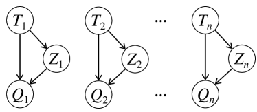
Figure 2: Bayesian network representation of $P$ as $\vec{T}$, $\vec{Z}$, and $\vec{Q}$.

It is not hard to verify that (unconditional) $Q_{j}$ follows the distribution $\pi$ over $\{R_{1},R_{2},R_{3},R_{4}\}$. Therefore $\vec{Q}$ follows the same distribution as $P$, which is $\pi^{n}$.

Step 2: Characterize the preference profiles.

In what follows, we characterize the event $\mathcal{E}_{1}$ where alternatives $1$ and $2$ are exactly tied and more agents prefer $(2\succ 1)$ than otherwise. That is, for $q\in[0,\frac{n}{6})$ and $\beta\in[q+1,2q]$, there are exactly:

• $\frac{n}{2}-q$ agents with rankings $R_{1}=[1\succ 2\succ 3]$ and $R_{2}=[2\succ 3\succ 1]$ each,

• $\beta$ agents with ranking $R_{3}=[3\succ 2\succ 1]$,

• $2q-\beta$ agents with ranking $R_{4}=[3\succ 1\succ 2]$.

We define the set $\mathcal{T}^{1,q}$ below to describes how many agents vote for each alternative. Next, we define the set $\mathcal{Z}_{\vec{t},\beta}$ to describe how many agents alternative $1$ or $2$ more, conditioned on $\vec{T}$. We use the Bayesian network framework from Step 1 and the law of total expectation to partition $\Pr(\mathcal{E}_{1})\times\mathbbm{E}[\text{D}^{+}(P)~{}|~{}\mathcal{E}_{1}]$ further according to these events. Note that we defer the other case, $\mathcal{E}_{2}$, where alternatives $1$ and $2$ are approximately tied and at least as many agents prefer $1\succ 2$ than otherwise, to Step 5 below.

Formally, let $\mathcal{T}^{1,q}\subseteq\{1,2,3\}^{n}$ denote the set of vectors $\vec{t}=(t_{1},\ldots,t_{n})$ such that alternatives $1$ and $2$ have the maximal plurality score of $\frac{n}{2}-q$ and alternative $1$ is the victor:

$$\mathcal{T}^{1,q}:=\left\{\vec{t}\in\{1,2,3\}^{n}~{}:~{}|\{j:t_{j}=1\}|=|\{j:t_{j}=2\}|=\left(\frac{n}{2}-q\right)>|\{j:t_{j}=3\}|\right\}.$$

It is easy to see that $\mathcal{E}_{1}$ holds for $\vec{Q}$ if and only if $\vec{T}$ takes a value in $\mathcal{T}^{1,q}$ for some $q\in\left[0,\frac{n}{6}\right)$. This implies the following equality:

$$\Pr(\mathcal{E}_{1})\times\mathbbm{E}[\text{D}^{+}(P)~{}|~{}\mathcal{E}_{1}]=\sum_{q=0}^{\frac{n}{6}-1}~{}\sum_{\vec{t}\in\mathcal{T}^{1,q}}\Pr(\vec{T}=\vec{t})\mathbbm{E}_{\vec{Q}}[\text{D}^{+}(\vec{Q})~{}|~{}\vec{T}=\vec{t}].$$ (11)

For any $\vec{t}\in\{1,2,3\}^{n}$, let

• $\text{Id}_{1}(\vec{t})\subseteq[n]$ denote the indices $j$ such that $t_{j}=1$,

• $\text{Id}_{2}(\vec{t})\subseteq[n]$ denote the indices $j$ such that $t_{j}=2$,

• $\text{Id}_{3}(\vec{t})\subseteq[n]$ denote the indices $j$ such that $t_{j}\notin\{1,2\}$ – we call these third-party agents.

For every $\beta\in\left[0,|\text{Id}_{3}(\vec{t})|\right]$, we define $\mathcal{Z}_{\vec{t},\beta}\subseteq\{1,2\}^{n}$ as the vectors $\vec{z}$ where the number of $2$s among indices in $\text{Id}_{3}(\vec{t})$ is exactly $\beta$:

$$\mathcal{Z}_{\vec{t},\beta}:=\{ \vec{z}\in\{1,2\}^{n}~{}:~{}\forall j\in\text{Id}_{1}(\vec{t})\cup\text{Id}_{2}(\vec{t}),z_{j}=t_{j},\text{ and }|\{j\in\text{Id}_{3}(\vec{t})~{}:~{}z_{j}=2\}|=\beta\}.$$

Notice that $\vec{t}\in\mathcal{T}^{1,q}$ implies $|\text{Id}_{1}(\vec{t})|=|\text{Id}_{2}(\vec{t})|$, so in order to uphold $\vec{Q}[2\succ 1]>\vec{Q}[1\succ 2]$, recalling Lemma 1 of [Kavner and Xia, 2021], there must be more third-party agents that prefer $(2\succ 1)$ than those that prefer $(1\succ 2)$. Since $|\text{Id}_{3}(\vec{t})|=2q$, we take $\beta\in\left[q+1,2q\right]$. Therefore, continuing Equation (11) we get:

$$\Pr(\mathcal{E}_{1})\times\mathbbm{E}[\text{D}^{+}(P)~{}|~{}\mathcal{E}_{1}]$$

$$=\sum_{q=0}^{\frac{n}{6}-1}~{}\sum_{\vec{t}\in\mathcal{T}^{1,q}}~{}\sum_{\beta=q+1}^{2q}~{}\sum_{\vec{z}\in\mathcal{Z}_{\vec{t},\beta}}\Pr(\vec{T}=\vec{t},\vec{Z}=\vec{z})\mathbbm{E}_{\vec{Q}}[\text{D}^{+}(\vec{Q})~{}|~{}\vec{T}=\vec{t},\vec{Z}=\vec{z}]$$

$$=\sum_{q=0}^{\frac{n}{6}-1}~{}\sum_{\vec{t}\in\mathcal{T}^{1,q}}~{}\sum_{\beta=q+1}^{2q}~{}\sum_{\vec{z}\in\mathcal{Z}_{\vec{t},\beta}}\Pr(\vec{T}=\vec{t},\vec{Z}=\vec{z})\sum_{j=1}^{n}\mathbbm{E}_{\vec{Q}_{j}}[\vec{u}(Q_{j},1)-\vec{u}(Q_{j},2)~{}|~{}\vec{T}=\vec{t},\vec{Z}=\vec{z}]$$

$$=\sum_{q=0}^{\frac{n}{6}-1}~{}\sum_{\vec{t}\in\mathcal{T}^{1,q}}~{}\sum_{\beta=q+1}^{2q}~{}\sum_{\vec{z}\in\mathcal{Z}_{\vec{t},\beta}}\Pr(\vec{T}=\vec{t},\vec{Z}=\vec{z})\sum_{j=1}^{n}E^{1}_{t_{j},z_{j}}$$ (12)

where

$$E^{1}_{t_{j},z_{j}}=\mathbbm{E}_{Q_{j}}[\vec{u}(Q_{j},1)-\vec{u}(Q_{j},2)~{}|~{}T_{j}=t_{j},Z_{j}=z_{j}].$$

This holds because of the Bayesian network structure: for any $j\leq n$, given $T_{j}$ and $Z_{j}$, $Q_{j}$ is independent of other $Q$’s.

Step 3: Substitute expected welfare per agent.

Note that $E^{1}_{t_{j},z_{j}}$ and only depends on the values of $t_{j}$ and $z_{j}$, but not $j$. By Assumption 1 and our use of Borda welfare, we have

$$E^{1}_{t_{j},z_{j}}=\begin{cases}1,&t_{j}=z_{j}=1\\ -2,&t_{j}=z_{j}=2\\ -1,&t_{j}\notin\{1,2\},z_{j}=2\\ 1,&t_{j}\notin\{1,2\},z_{j}=1.\end{cases}$$

That is, each agent $j$ with $t_{j}=1$ as their most-preferred alternative must have ranking $R_{j}=R_{1}=[1\succ 2\succ 3]$. This entails that they contribute $\vec{u}(R_{1},1)-\vec{u}(R_{1},2)=1$ Borda welfare to the adversarial loss $\text{D}^{+}(\vec{Q})$. The same argument holds for $-2$ Borda welfare when $t_{j}=2$, corresponding with $R_{2}=[2\succ 3\succ 1]$. Next, any agent with $t_{j}\notin\{1,2\}$ entails that they have either ranking $R_{3}=[3\succ 2\succ 1]$ or $R_{4}=[3\succ 1\succ 2]$. If $z_{j}=2$, they have ranking $R_{3}$ and contribute $-1$ Borda welfare to $\text{D}^{+}(\vec{Q})$; otherwise, if $z_{j}=1$, they have ranking $R_{4}$ and contribute $1$ Borda welfare.

Equation (12) therefore becomes:

$$\sum_{q=0}^{\frac{n}{6}-1}~{}\sum_{\vec{t}\in\mathcal{T}^{1,q}}~{}\sum_{\beta=q+1}^{2q}~{}\sum_{\vec{z}\in\mathcal{Z}_{\vec{t},\beta}}\Pr(\vec{T}=\vec{t},\vec{Z}=\vec{z})\left(\left(\frac{n}{2}-q,\frac{n}{2}-q,\beta,2q-\beta\right)\cdot(1,-2,-1,1)\right)$$

$$=\sum_{q=0}^{\frac{n}{6}-1}~{}\sum_{\vec{t}\in\mathcal{T}^{1,q}}~{}\sum_{\beta=q+1}^{2q}~{}\sum_{\vec{z}\in\mathcal{Z}_{\vec{t},\beta}}\Pr(\vec{T}=\vec{t},\vec{Z}=\vec{z})\left(-\frac{n}{2}+3q-2\beta\right)$$

$$=\sum_{q=0}^{\frac{n}{6}-1}~{}\sum_{\vec{t}\in\mathcal{T}^{1,q}}\Pr(\vec{T}=\vec{t})\sum_{\beta=q+1}^{2q}\left(-\frac{n}{2}+3q-2\beta\right)\sum_{\vec{z}\in\mathcal{Z}_{\vec{t},\beta}}\Pr(\vec{Z}=\vec{z}~{}|~{}\vec{T}=\vec{t})$$

$$=\sum_{q=0}^{\frac{n}{6}-1}~{}\sum_{\vec{t}\in\mathcal{T}^{1,q}}\Pr(\vec{T}=\vec{t})\sum_{\beta=q+1}^{2q}\left(-\frac{n}{2}+3q-2\beta\right)\binom{2q}{\beta}\frac{1}{2^{2q}}$$ (13)

where the last line follows from

$$\Pr(Z_{j}=1~{}|~{}T_{j}\notin\{1,2\})=0.5.$$

Case when $q=0$.

Notice that Equation (13) is zero when $q=0$. This is because there are zero third-party agents, so there is no IV dynamics. By Lemma 1 of [Kavner and Xia, 2021] the adversarial loss is zero.

Next, we make use of the following binomial identities, which are proved in Appendix F.

Lemma 3.

For $q\geq 1$, the following identities hold:

1. $$\sum_{\beta=q+1}^{2q}\binom{2q}{\beta}\frac{1}{2^{2q}}=\frac{1}{2}-\frac{1}{2^{2q}}\binom{2q-1}{q-1}$$

2. $$\sum_{\beta=q+1}^{2q}\beta\binom{2q}{\beta}\frac{1}{2^{2q}}=\frac{q}{2}$$

By applying Equations 1 and 2 of Lemma 3, Equation (13) simplifies to

$$\sum_{q=1}^{\frac{n}{6}-1}~{}\sum_{\vec{t}\in\mathcal{T}^{1,q}}\Pr(\vec{T}=\vec{t})\left(\left(-\frac{n}{2}+3q\right)\left(\frac{1}{2}-\frac{1}{2^{2q}}\binom{2q-1}{q-1}\right)-2\left(\frac{q}{2}\right)\right)$$

$$=\sum_{q=1}^{\frac{n}{6}-1}\left(\frac{1}{2}\left(-\frac{n}{2}+q\right)-\left(\frac{\left(-\frac{n}{2}+3q\right)}{2^{2q}}\binom{2q-1}{q-1}\right)\right)\Pr(\vec{T}\in\mathcal{T}^{1,q}).$$ (14)

Recall that $\vec{T}$ is a multinomial distribution over $\{1,2,3\}$ with event probabilities $(\pi_{1},\pi_{2},\pi_{3}+\pi_{4})$. Furthermore, $\mathcal{T}^{1,q}$ is the event where there are $\frac{n}{2}-q$ of $1s$ and $2s$ each in $\vec{T}$, and $2q$ of $3s$. Therefore

$$\Pr(\vec{T}\in\mathcal{T}^{1,q}) =\binom{n}{\frac{n}{2}-q,\frac{n}{2}-q,2q}\pi_{1}^{\frac{n}{2}-q}\pi_{2}^{\frac{n}{2}-q}(\pi_{3}+\pi_{4})^{2q}$$

$$=\binom{n}{\frac{n}{2}-q,\frac{n}{2}-q,q,q}\pi_{1}^{n-2q}\pi_{3}^{2q}\cdot\frac{2^{2q}}{\binom{2q}{q}}.$$ (15)

Hence, Equation (14) becomes

$$\sum_{q=1}^{\frac{n}{6}-1}\binom{n}{\frac{n}{2}-q,\frac{n}{2}-q,q,q}\pi_{1}^{n-2q}\pi_{3}^{2q}\left(\frac{\left(-\frac{n}{2}+q\right)}{2}\frac{2^{2q}}{\binom{2q}{q}}-\frac{\left(-\frac{n}{2}+3q\right)}{2}\right)$$ (16)

where we use the fact that $2\binom{2q-1}{q-1}=\binom{2q}{q}$.

Step 4: Repeat process for $\mathcal{E}_{2}$.

We next repeat the above process in Steps 2 and 3 for $\mathcal{E}_{2}$, where alternatives $1$ and $2$ are approximately tied and at least as many agents prefer $(1\succ 2)$ than otherwise.

Let $\mathcal{T}^{2,q}\subseteq[3]^{n}$ denote the set of vectors $\vec{t}=(t_{1},\ldots,t_{n})$ such that alternative $2$ has the maximal plurality score of $\frac{n}{2}-q$ and alternative $1$ has one fewer vote:

$$\mathcal{T}^{2,q}:=\left\{\vec{t}\in[3]^{n}~{}:~{}|\{j:t_{j}=1\}|+1=|\{j:t_{j}=2\}|=\left(\frac{n}{2}-q\right)>|\{j:t_{j}=3\}|\right\}.$$

It is easy to see that $\mathcal{E}_{2}$ holds for $\vec{Q}$ if and only if $\vec{T}$ takes a value in $\mathcal{T}^{2,q}$ for some $q\in\left[0,\frac{n}{6}\right)$. This implies the following equality:

$$\Pr(\mathcal{E}_{2})\times\mathbbm{E}[\text{D}^{+}(P)~{}|~{}\mathcal{E}_{2}]=\sum_{q=0}^{\frac{n}{6}-1}~{}\sum_{\vec{t}\in\mathcal{T}^{2,q}}\Pr(\vec{T}=\vec{t})\mathbbm{E}_{\vec{Q}}[\text{D}^{+}(\vec{Q})~{}|~{}\vec{T}=\vec{t}].$$ (17)

Recall the definitions of $\text{Id}_{1}(\vec{t})$, $\text{Id}_{2}(\vec{t})$, $\text{Id}_{3}(\vec{t})$, and $\mathcal{Z}_{\vec{t},\beta}$ above. Notice that $\vec{t}\in\mathcal{T}^{2,q}$ implies $|\text{Id}_{1}(\vec{t})|+1=|\text{Id}_{2}(\vec{t})|$, so in order to uphold $\vec{Q}[1\succ 2]\geq\vec{Q}[2\succ 1]$ there must be at least as many third-party agents that prefer $(1\succ 2)$ than those that prefer $(2\succ 1)$. Since $|\text{Id}_{3}(\vec{t})|=2q+1$, we take $\beta\in\left[0,q\right]$. Therefore, continuing Equation (17) we get:

$$\Pr(\mathcal{E}_{2})\times\mathbbm{E}[\text{D}^{+}(P)~{}|~{}\mathcal{E}_{2}]$$

$$=\sum_{q=0}^{\frac{n}{6}-1}~{}\sum_{\vec{t}\in\mathcal{T}^{2,q}}~{}\sum_{\beta=0}^{q}~{}\sum_{\vec{z}\in\mathcal{Z}_{\vec{t},\beta}}\Pr(\vec{T}=\vec{t},\vec{Z}=\vec{z})\mathbbm{E}_{\vec{Q}}[\text{D}^{+}(\vec{Q})~{}|~{}\vec{T}=\vec{t},\vec{Z}=\vec{z}]$$

$$=\sum_{q=0}^{\frac{n}{6}-1}~{}\sum_{\vec{t}\in\mathcal{T}^{2,q}}~{}\sum_{\beta=0}^{q}~{}\sum_{\vec{z}\in\mathcal{Z}_{\vec{t},\beta}}\Pr(\vec{T}=\vec{t},\vec{Z}=\vec{z})\sum_{j=1}^{n}\mathbbm{E}_{\vec{Q}_{j}}[\vec{u}(Q_{j},2)-\vec{u}(Q_{j},1)~{}|~{}\vec{T}=\vec{t},\vec{Z}=\vec{z}]$$

$$=\sum_{q=0}^{\frac{n}{6}-1}~{}\sum_{\vec{t}\in\mathcal{T}^{2,q}}~{}\sum_{\beta=0}^{q}~{}\sum_{\vec{z}\in\mathcal{Z}_{\vec{t},\beta}}\Pr(\vec{T}=\vec{t},\vec{Z}=\vec{z})\sum_{j=1}^{n}E^{2}_{t_{j},z_{j}}$$ (18)

where

$$E^{2}_{t_{j},z_{j}}=\mathbbm{E}_{\vec{Q}_{j}}[\vec{u}(Q_{j},2)-\vec{u}(Q_{j},1)~{}|~{}T_{j}=t_{j},Z_{j}=z_{j}]$$

which holds because of the Bayesian network structure. Notice that $E^{2}_{t_{j},z_{j}}$ and only depends on the values of $t_{j}$ and $z_{j}$, but not $j$. By Assumption 1, our use of Borda welfare, and realizing that $E^{1}_{t_{j},z_{j}}=-E^{2}_{t_{j},z_{j}}$, Equation (18) becomes:

$$\sum_{q=0}^{\frac{n}{6}-1}~{}\sum_{\vec{t}\in\mathcal{T}^{2,q}}~{}\sum_{\beta=0}^{q}~{}\sum_{\vec{z}\in\mathcal{Z}_{\vec{t},\beta}}\Pr(\vec{T}=\vec{t},\vec{Z}=\vec{z})\left(\left(\frac{n}{2}-1-q,\frac{n}{2}-q,\beta,2q+1-\beta\right)\cdot-(1,-2,-1,1)\right)$$

$$=-\sum_{q=0}^{\frac{n}{6}-1}~{}\sum_{\vec{t}\in\mathcal{T}^{2,q}}~{}\sum_{\beta=0}^{q}~{}\sum_{\vec{z}\in\mathcal{Z}_{\vec{t},\beta}}\Pr(\vec{T}=\vec{t},\vec{Z}=\vec{z})\left(-\frac{n}{2}+3q-2\beta\right)$$

$$=-\sum_{q=0}^{\frac{n}{6}-1}~{}\sum_{\vec{t}\in\mathcal{T}^{2,q}}\Pr(\vec{T}=\vec{t})\sum_{\beta=0}^{q}\left(-\frac{n}{2}+3q-2\beta\right)\sum_{\vec{z}\in\mathcal{Z}_{\vec{t},\beta}}\Pr(\vec{Z}=\vec{z}~{}|~{}\vec{T}=\vec{t})$$

$$=-\sum_{q=0}^{\frac{n}{6}-1}~{}\sum_{\vec{t}\in\mathcal{T}^{2,q}}\Pr(\vec{T}=\vec{t})\sum_{\beta=0}^{q}\left(-\frac{n}{2}+3q-2\beta\right)\binom{2q+1}{\beta}\frac{1}{2^{2q+1}}$$ (19)

since

$$\Pr(Z_{j}=1~{}|~{}T_{j}\notin\{1,2\})=0.5.$$

Case when $q=0$.

For Equation (19), when $q=0$ we have $\beta=0$, so this becomes

$$\sum_{\vec{t}\in\mathcal{T}^{2,0}}\Pr(\vec{T}=\vec{t})\cdot\left(-\frac{n}{2}\right)\binom{1}{0}\frac{1}{2}$$

$$=-\frac{n}{4}\Pr(\vec{T}\in\mathcal{T}^{2,0})$$

$$=-\frac{n}{4}\binom{n}{\frac{n}{2}-1,\frac{n}{2},1}\pi_{1}^{\frac{n}{2}-1}\pi_{2}^{\frac{n}{2}}(\pi_{3}+\pi_{4})^{1}$$

$$=-\frac{n\pi_{3}\pi_{1}^{n}}{2\pi_{1}}(n/2)\binom{n}{n/2}$$

$$=-\mathcal{O}(n^{1.5})\cdot(2\pi_{1})^{n}$$

$$=-\exp(-\Theta(n))$$

by Stirling’s approximation (Proposition 2).

Proposition 2 (Stirling’s approximation).

$$n!\sim\sqrt{2\pi n}\left(\frac{n}{e}\right)^{n}.$$

Hence,

$$\binom{2n}{n}\sim\frac{2^{2n}}{\sqrt{n\pi}}.$$

This proposition is discussed further in Appendix E.

Next, we make use of the following binomial identities, which are proved in Appendix F

Lemma 3.

For $q\geq 1$, the following identities hold:

1. $$\sum_{\beta=0}^{q}\binom{2q+1}{\beta}\frac{1}{2^{2q+1}}=\frac{1}{2}$$

2. $$\sum_{\beta=0}^{q}\beta\binom{2q+1}{\beta}\frac{1}{2^{2q+1}}=\left(\frac{2q+1}{4}\right)-\frac{2q+1}{2^{2q+1}}\binom{2q-1}{q-1}.$$

By applying Equations 3 and 4 of Lemma 3, Equation (19) simplifies to

$$-\sum_{q=1}^{\frac{n}{6}-1}~{}\sum_{\vec{t}\in\mathcal{T}^{2,q}}\Pr(\vec{T}=\vec{t})\left(\left(-\frac{n}{2}+3q\right)\left(\frac{1}{2}\right)-2\left(\frac{2q+1}{4}-\frac{2q+1}{2^{2q+1}}\binom{2q-1}{q-1}\right)\right)$$

$$=-\sum_{q=1}^{\frac{n}{6}-1}\left(\frac{1}{2}\left(-\frac{n}{2}+q-1\right)+\frac{2q+1}{2^{2q}}\binom{2q-1}{q-1}\right)\Pr(\vec{T}\in\mathcal{T}^{2,q}).$$ (20)

Recall that $\mathcal{T}^{2,q}$ is the event where there are $\frac{n}{2}-1-q$ of $1s$ in $\vec{T}$, $\frac{n}{2}-q$ and $2s$, and $2q+1$ of $3s$. Therefore,

$$\Pr(\vec{T}\in\mathcal{T}^{2,q}) =\binom{n}{\frac{n}{2}-1-q,\frac{n}{2}-q,2q+1}\pi_{1}^{\frac{n}{2}-1-q}\pi_{2}^{\frac{n}{2}-q}(\pi_{3}+\pi_{4})^{2q+1}$$

$$=\binom{n}{\frac{n}{2}-q,\frac{n}{2}-q,q,q}\pi_{1}^{n-2q}\pi_{3}^{2q}\cdot\frac{\pi_{3}(\frac{n}{2}-q)}{\pi_{1}(2q+1)}\frac{2^{2q+1}}{\binom{2q}{q}}.$$ (21)

Hence, Equation (20) becomes

$$-\sum_{q=1}^{\frac{n}{6}-1}\binom{n}{\frac{n}{2}-q,\frac{n}{2}-q,q,q}\pi_{1}^{n-2q}\pi_{3}^{2q}\left(\frac{\pi_{3}(-\frac{n}{2}+q-1)(\frac{n}{2}-q)}{\pi_{1}(2q+1)}\frac{2^{2q}}{\binom{2q}{q}}+\frac{\pi_{3}(\frac{n}{2}-q)}{\pi_{1}}\right)$$ (22)

where we again use the fact that $2\binom{2q-1}{q-1}=\binom{2q}{q}$.

Step 5: Put parts together.

Recall that our original problem began as Equation (10) which we initially split into Equation (11) and (17). Through a sequence of steps we transformed these equations into (16) and (22). Recombining them yields

$$\sum_{q=1}^{\frac{n}{6}-1}\binom{n}{\frac{n}{2}-q,\frac{n}{2}-q,q,q}\pi_{1}^{n-2q}\pi_{3}^{2q}\left(-\frac{1}{2}\left(-\frac{n}{2}+3q\right)+\frac{\pi_{3}}{\pi_{1}}\left(-\frac{n}{2}+q\right)\right)$$

$$+\sum_{q=1}^{\frac{n}{6}-1}\binom{n}{\frac{n}{2}-q,\frac{n}{2}-q,q,q}\pi_{1}^{n-2q}\pi_{3}^{2q}\frac{(-\frac{n}{2}+q)2^{2q}}{\binom{2q}{q}}\left(\frac{1}{2}+\frac{\pi_{3}(-\frac{n}{2}+q-1)}{\pi_{1}(2q+1)}\right).$$ (23)

In Appendix B we introduce Lemma 4 to analyze the asymptotic rate of the first summation of Equation (23) and Lemma 7 to analyze the second summation. Lemma 2 follows from these two lemmas. ∎

Appendix B Multinomial Lemmas

Lemma 4.

$$\sum_{q=1}^{\frac{n}{6}-1}\binom{n}{\frac{n}{2}-q,\frac{n}{2}-q,q,q}\pi_{1}^{n-2q}\pi_{3}^{2q}\left(-\frac{1}{2}\left(-\frac{n}{2}+3q\right)+\frac{\pi_{3}}{\pi_{1}}\left(-\frac{n}{2}+q\right)\right)=\begin{cases}\Theta\left(1\right),&\pi_{1}<0.4\\ -\Theta\left(1\right),&\pi_{1}>0.4\\ \pm\mathcal{O}\left(\frac{1}{n}\right),&\pi_{1}=0.4.\end{cases}$$

Proof.

Notice that the objective takes the same form as the evaluation of a discrete expected value: it is a summation over the range of $q$ of a multinomial likelihood, indexed by $q$, multiplied by the score function

$$f_{n}(q):=-\frac{1}{2}\left(-\frac{n}{2}+3q\right)+\frac{\pi_{3}}{\pi_{1}}\left(-\frac{n}{2}+q\right).$$

This function is bounded by $\pm\mathcal{O}(n)$ and is monotonic in $q$ for fixed $n$. We prove the lemma by partitioning the summation into different ranges of $q$ and handling each case differently. We see that for small enough $q$, $f_{n}(q)=-\Theta(n)$, so we can factor it out of the objective and evaluate the sum of probabilities. We make use Lemma 5, which applies a theorem from [Xia, 2021a], to evaluate this remaining sum as either $\mathcal{O}\left(\frac{1}{n}\right)$ or $\exp(-\Theta(n))$ depending on where we partition the objective. A similar case holds for large enough $q$, where $f_{n}(q)=\Theta(n)$.

Now, the place at which we partition the objective summation depends on $\pi_{1}$. When $\pi_{1}>0.4$ we ntoice that $f_{n}(q)>0\iff q>\epsilon\pi_{3}n$ for some $\epsilon>1$. Hence, we can partition the summation at the point $\frac{(\epsilon+1)}{2}\pi_{3}n$ and employ Lemma 5 on these segments separately. A similar process holds for $\pi_{1}<0.4$ to partition the summation at $\epsilon\pi_{3}n$ for $\epsilon<1$. However, a different technique must be used when $\pi_{1}=0.4$. We first recognize that $f_{n}(q)=\frac{5}{4}(\pi_{3}n-q)$. We have $f_{n}(q)\in[-\mathcal{O}(n),\mathcal{O}(n)]$, so we cannot immediately factor it out of the objective summation. We treat this case separately as Lemma 6. The technical details are as follows.

Initial observations.

Notice that

$$f_{n}(q)>0\iff q>\frac{n\left(\frac{1}{2}-\frac{\pi_{3}}{\pi_{1}}\right)}{2\left(\frac{3}{2}-\frac{\pi_{3}}{\pi_{1}}\right)}.$$

It is easy to verify that $\frac{n\left(\frac{1}{2}-\frac{\pi_{3}}{\pi_{1}}\right)}{2\left(\frac{3}{2}-\frac{\pi_{3}}{\pi_{1}}\right)}<\frac{n}{6}$ since $\pi_{3}>0$. Let $\epsilon=\frac{1}{2\pi_{3}}\left(\frac{1-6\pi_{3}}{3-10\pi_{3}}\right)$ such that

$$\epsilon\pi_{3}n=\frac{n\left(\frac{1}{2}-\frac{\pi_{3}}{\pi_{1}}\right)}{2\left(\frac{3}{2}-\frac{\pi_{3}}{\pi_{1}}\right)}.$$

Recall that $\pi_{3}\in(0,\frac{1}{6})$ and $\pi_{1}=\frac{1}{2}-\pi_{3}$ by Assumption 1, so $\epsilon>0$. Hence:

• $\epsilon>1$ if and only if $\pi_{3}<0.1$,

• $\epsilon<1$ if and only if $\pi_{3}>0.1$,

• $\epsilon=1$ if and only if $\pi_{3}=0.1$.

This entails three cases to the lemma.

Case 1: ($\pi_{3}<0.1$).

Suppose first that $\pi_{3}<0.1$ so that $\epsilon>1$. Then $f_{n}(q)>0\iff q>\epsilon\pi_{3}n$. We partition the summation

$$\sum_{q=1}^{\frac{n}{6}-1}\binom{n}{\frac{n}{2}-q,\frac{n}{2}-q,q,q}\pi_{1}^{n-2q}\pi_{3}^{2q}f_{n}(q)$$

$$=-\Theta(n)\sum_{q=1}^{\left\lceil\frac{(\epsilon+1)}{2}\pi_{3}n\right\rceil}\binom{n}{\frac{n}{2}-q,\frac{n}{2}-q,q,q}\pi_{1}^{n-2q}\pi_{3}^{2q}$$

$$\quad\quad-\Theta(n)\sum_{q=\left\lceil\frac{(\epsilon+1)}{2}\pi_{3}n\right\rceil+1}^{\left\lceil\epsilon\pi_{3}n\right\rceil}\binom{n}{\frac{n}{2}-q,\frac{n}{2}-q,q,q}\pi_{1}^{n-2q}\pi_{3}^{2q}$$

$$\quad\quad+\Theta(n)\sum_{q=\left\lceil\epsilon\pi_{3}n\right\rceil+1}^{\frac{n}{6}-1}\binom{n}{\frac{n}{2}-q,\frac{n}{2}-q,q,q}\pi_{1}^{n-2q}\pi_{3}^{2q}$$

$$=-\Theta(n)\Theta\left(\frac{1}{n}\right)-\exp(-\Theta(n))+\exp(-\Theta(n))$$

$$=-\Theta(1)$$

by Lemma 5. This lemma is a direct application of Theorem 1 from [Xia, 2021a] and is proved in Appendix C.

Lemma 5.

Fix $a,b\in(0,\frac{1}{6})$, $a<b$. Then

$$\sum_{q=\left\lfloor an\right\rfloor}^{\frac{n}{6}-1}\binom{n}{\frac{n}{2}-q,\frac{n}{2}-q,q,q}\pi_{1}^{n-2q}\pi_{3}^{2q}=\begin{cases}\Theta\left(\frac{1}{n}\right),&\pi_{3}\geq a\\ \exp(-\Theta(n)),&\text{otherwise}\end{cases}$$

and

$$\sum_{q=1}^{\left\lceil bn\right\rceil}\binom{n}{\frac{n}{2}-q,\frac{n}{2}-q,q,q}\pi_{1}^{n-2q}\pi_{3}^{2q}=\begin{cases}\Theta\left(\frac{1}{n}\right),&\pi_{3}\leq b\\ \exp(-\Theta(n)),&\text{otherwise}.\end{cases}$$

Case 2: ($\pi_{3}>0.1$).

Now suppose that $\pi_{3}>0.1$ so that $\epsilon<1$. Then $f_{n}(q)<0\iff q<\epsilon\pi_{3}n$. Like the first case, we get by applying Lemma 5 that

$$\sum_{q=1}^{\frac{n}{6}-1}\binom{n}{\frac{n}{2}-q,\frac{n}{2}-q,q,q}\pi_{1}^{n-2q}\pi_{3}^{2q}f_{n}(q)$$

$$=-\Theta(n)\sum_{q=1}^{\left\lfloor\epsilon\pi_{3}n\right\rfloor-1}\binom{n}{\frac{n}{2}-q,\frac{n}{2}-q,q,q}\pi_{1}^{n-2q}\pi_{3}^{2q}$$

$$\quad\quad+\Theta(n)\sum_{q=\left\lfloor\epsilon\pi_{3}n\right\rfloor}^{\left\lfloor\frac{(\epsilon+1)}{2}\pi_{3}n\right\rfloor-1}\binom{n}{\frac{n}{2}-q,\frac{n}{2}-q,q,q}\pi_{1}^{n-2q}\pi_{3}^{2q}$$

$$\quad\quad+\Theta(n)\sum_{q=\left\lfloor\frac{(\epsilon+1)}{2}\pi_{3}n\right\rfloor}^{\frac{n}{6}-1}\binom{n}{\frac{n}{2}-q,\frac{n}{2}-q,q,q}\pi_{1}^{n-2q}\pi_{3}^{2q}$$

$$=-\exp(-\Theta(n))+\exp(-\Theta(n))+\Theta(n)\Theta\left(\frac{1}{n}\right)$$

$$=\Theta(1).$$

Case 3: ($\pi_{3}=0.1$).

In the final case, in which $\pi_{3}=0.1$, we have

$$f_{n}(q)=\frac{1}{4}\left(\frac{n}{2}-5q\right)=\frac{5}{4}\left(\pi_{3}n-q\right).$$

Therefore the objective becomes

$$\frac{5}{4}\sum_{q=1}^{\frac{n}{6}-1}\binom{n}{\frac{n}{2}-q,\frac{n}{2}-q,q,q}\pi_{1}^{n-2q}\pi_{3}^{2q}(\pi_{3}n-q)$$

$$=-\frac{5\binom{n}{\frac{n}{2}}\sqrt{2n\pi_{3}\pi_{1}}}{2^{n+2}}\sum_{q=1}^{\frac{n}{6}-1}\left(\binom{\frac{n}{2}}{q}(2\pi_{1})^{\frac{n}{2}-q}(2\pi_{3})^{q}\right)^{2}\frac{(q-\pi_{3}n)}{\sqrt{2n\pi_{3}\pi_{1}}}$$ (24)

by Proposition 1, which is proved in Appendix F.

Proposition 1.

Let $q\in\left[1,\frac{n}{6}-1\right]$. Then

$$\binom{n}{\frac{n}{2}-q,\frac{n}{2}-q,q,q}\pi_{1}^{n-2q}\pi_{3}^{2q}=\frac{\binom{n}{\frac{n}{2}}}{2^{n}}\left(\binom{\frac{n}{2}}{q}(2\pi_{1})^{\frac{n}{2}-q}(2\pi_{3})^{q}\right)^{2}.$$

This proposition is useful for transforming the multinomial likelihood to a squared-binomial equivalence. The factor out-front is $\Theta\left(\frac{1}{\sqrt{n}}\right)$ by Stirling’s approximation (see Proposition 2 in Appendix E). Notice that the multinomial domain of $q$ is $[0,\frac{n}{6}]$ while the binomial domain of $q$ is $[0,\frac{n}{2}]$. We may therefore extend the range of Equation (24) by adding a summation which is exponentially small by Hoeffding’s inequality (Proposition 3). That is, Equation (24) can be written as

$$\Theta(1)\sum_{q=\frac{n}{6}}^{\frac{n}{2}}\left(\binom{\frac{n}{2}}{q}(2\pi_{1})^{\frac{n}{2}-q}(2\pi_{3})^{q}\right)^{2}\frac{(q-\pi_{3}n)}{\sqrt{2n\pi_{3}\pi_{1}}}$$

$$\quad\quad+\Theta(1)\left[\left(\binom{\frac{n}{2}}{0}(2\pi_{1})^{\frac{n}{2}-0}(2\pi_{3})^{0}\right)^{2}\frac{(0-\pi_{3}n)}{\sqrt{2n\pi_{3}\pi_{1}}}\right]$$

$$\quad\quad-\Theta(1)\sum_{q=0}^{\frac{n}{2}}\left(\binom{\frac{n}{2}}{q}(2\pi_{1})^{\frac{n}{2}-q}(2\pi_{3})^{q}\right)^{2}\frac{(q-\pi_{3}n)}{\sqrt{2n\pi_{3}\pi_{1}}}$$

$$=\pm\exp(-\Theta(n))-\Theta(1)\sum_{q=0}^{\frac{n}{2}}\left(\binom{\frac{n}{2}}{q}(2\pi_{1})^{\frac{n}{2}-q}(2\pi_{3})^{q}\right)^{2}\frac{(q-\pi_{3}n)}{\sqrt{2n\pi_{3}\pi_{1}}}.$$ (25)

Proposition 3 (Hoeffding’s Inequality).

Let $p\in(0,1)$ and $q=1-p$; let $a,b\in\mathbb{R}$ such that $0\leq a<b\leq 1$. If $p\notin[a,b]$ then

$$\sum_{k=\left\lfloor an\right\rfloor}^{\left\lceil bn\right\rceil}\left(\binom{n}{k}p^{n-k}q^{k}\right)^{2}=\exp(-\Theta(n)).$$

Our specific use of this inequality is proved in Appendix F. Finally, Equation (25) leads to

$$\pm\exp(-\Theta(n))\pm\Theta(1)\mathcal{O}\left(\frac{1}{n}\right)=\pm\mathcal{O}\left(\frac{1}{n}\right)$$

by Lemma 6, which is proved in Appendix D. In that appendix, we discuss the necessary change of variables in order to apply the lemma. Simply put, we exchange $\frac{n}{2}\mapsto n$ and $2\pi_{3}\mapsto p$.

Lemma 6.

Let $p\in(0,\frac{2}{3})$ and $S_{n}\sim Bin(n,p)$. Then

$$\left|\sum_{k=0}^{n}\left(\frac{k-np}{\sqrt{np(1-p)}}\right)\Pr(S_{n}=k)^{2}\right|=\mathcal{O}\left(\frac{1}{n}\right).$$

This concludes the proof of Lemma 4. ∎

Lemma 7.

$$\left|\sum_{q=1}^{\frac{n}{6}-1}\binom{n}{\frac{n}{2}-q,\frac{n}{2}-q,q,q}\pi_{1}^{n-2q}\pi_{3}^{2q}\frac{(-\frac{n}{2}+q)2^{2q}}{\binom{2q}{q}}\left(\frac{1}{2}+\frac{\pi_{3}(-\frac{n}{2}+q-1)}{\pi_{1}(2q+1)}\right)\right|=\mathcal{O}\left(\frac{1}{\sqrt{n}}\right).$$

Proof.

Throughout this proof we will use the fact that:

$$\left(-\frac{n}{2}+q\right)\left(\frac{1}{2}+\frac{\pi_{3}(-\frac{n}{2}+q-1)}{\pi_{1}(2q+1)}\right)$$ (26)

$$=\frac{1}{2\pi_{1}(2q+1)}\left(-\frac{n}{2}+q\right)\left(q-\pi_{3}n+\pi_{1}-2\pi_{3}\right)$$

$$=\frac{1}{2\pi_{1}(2q+1)}\left((q-\pi_{3}n)^{2}+(q-\pi_{3}n)(-\pi_{1}n+\pi_{1}-2\pi_{3})+(-\pi_{1}n)(\pi_{1}-2\pi_{3})\right)$$ (27)

where $\pi_{1}-2\pi_{3}\in(0,\frac{1}{2})$ by Assumption 1. Let

$$f_{n}(q):=\left(-\frac{n}{2}+q\right)\left(q-\pi_{3}n+\pi_{1}-2\pi_{3}\right)$$

so that, in the objective,

$$\frac{(-\frac{n}{2}+q)2^{2q}}{\binom{2q}{q}}\left(\frac{1}{2}+\frac{\pi_{3}(-\frac{n}{2}+q-1)}{\pi_{1}(2q+1)}\right)=\frac{f_{n}(q)}{2\pi_{1}}\frac{2^{2q}}{(2q+1)\binom{2q}{q}}.$$

It is clear that $f_{n}(q)$ is $+\Theta(n^{2})$ or $-\mathcal{O}(n^{2})$ when $q-\pi_{3}n$ is $-\Theta(n)$ or $+\Theta(n)$, respectively. Therefore we may expect to be able to factor out $f_{n}(q)$ from the objective when $q$ is either small- or large-enough. However, it is initially unclear how to treat $f_{n}(q)$ when $q$ is near the “center” of the summation since $f_{n}(q)$ switches signs. Recall from Proposition 1 that the likelihood term in the objective, $\binom{n}{\frac{n}{2}-q,\frac{n}{2}-q,q,q}\pi_{1}^{n-2q}\pi_{3}^{2q}$, is equivalent to $\mathcal{O}\left(\frac{1}{\sqrt{n}}\right)\times$ the squared-binomial probability centered at $\pi_{3}n$. The “center” of the summation, therefore, is when $q$ is $o(n)$ away from $\pi_{3}n$.

To handle these separate cases, we partition the objective summation region $[1,\frac{n}{6})$ into three regions defined below:

1. a “small-$q$” region, $A_{n}$, covering $[1,\frac{\pi_{3}n}{2})$,

2. a “large-$q$” region, $B_{n}$, covering (the negation of) $[\frac{n}{6},\frac{n}{2}]$,

3. the remainder, $C_{n}$, covering $[\frac{\pi_{3}n}{2},\frac{n}{2}]$.

Both $A_{n}$ and $B_{n}$ are $\Theta(n)$ in size but do not cover the center $\pi_{3}n$. Therefore, by Hoeffding’s inequality (Proposition 3) and Lemma 5, these terms are exponentially small. Analyzing $C_{n}$ requires a different technique using the definition of $f_{n}(q)$. From Equation (27) above, we see that there are three terms with varying powers of $(q-\pi_{3}n)^{k}$, $k\in\{2,1,0\}$. These three terms split up $C_{n}$ into three further sub-equations, $D_{n}$, $E_{n}$, and $F_{n}$, respectively. We make use of Lemmas 9 and 10 below to analyze two of these equations, while the third is analyzed using properties of the additional term $\frac{2^{2q}}{(2q+1)\binom{2q}{q}}\times\mathcal{O}\left(\frac{1}{\sqrt{n}}\right)$ from Proposition 1, and Lemma 5. The technical details are as follows.

We start off by splitting up the objective into three parts:

$$A_{n}+B_{n}+C_{n}$$ (28)

where we define

$$A_{n} =\sum_{q=1}^{\left\lfloor\frac{\pi_{3}n}{2}\right\rfloor-1}\binom{n}{\frac{n}{2}-q,\frac{n}{2}-q,q,q}\pi_{1}^{n-2q}\pi_{3}^{2q}\frac{f_{n}(q)}{2\pi_{1}}\frac{2^{2q}}{(2q+1)\binom{2q}{q}},$$

$$B_{n} =-\frac{\binom{n}{\frac{n}{2}}}{2^{n}}\sum_{q=\frac{n}{6}}^{\frac{n}{2}}\left(\binom{\frac{n}{2}}{q}(2\pi_{1})^{\frac{n}{2}-q}(2\pi_{3})^{q}\right)^{2}\frac{f_{n}(q)}{2\pi_{1}}\frac{2^{2q}}{(2q+1)\binom{2q}{q}},$$

$$C_{n} =\frac{\binom{n}{\frac{n}{2}}}{2^{n}}\sum_{q=\left\lfloor\frac{\pi_{3}n}{2}\right\rfloor}^{\frac{n}{2}}\left(\binom{\frac{n}{2}}{q}(2\pi_{1})^{\frac{n}{2}-q}(2\pi_{3})^{q}\right)^{2}\frac{f_{n}(q)}{2\pi_{1}}\frac{2^{2q}}{(2q+1)\binom{2q}{q}},$$

making use of Proposition 1, while adding and subtracting the same terms over the regions $q\in[\frac{n}{6},\frac{n}{2}]$ to make $B_{n}$ and $C_{n}$.

Consider the first summation of Equation (28). Notice that $f_{n}(q)=\Theta(n^{2})$ along the domain $q\in[1,\left\lfloor\frac{\pi_{3}n}{2}\right\rfloor-1]$, that $\frac{2^{2q}}{\binom{2q}{q}(2q+1)}\in(0,1)$, $\forall q>0$, and that $\frac{2^{2q}}{\binom{2q}{q}(2q+1)}$ is decreasing in $q$ by Stirling’s approximation (Proposition 2). Therefore,

$$A_{n} =\sum_{q=1}^{\left\lfloor\frac{\pi_{3}n}{2}\right\rfloor-1}\binom{n}{\frac{n}{2}-q,\frac{n}{2}-q,q,q}\pi_{1}^{n-2q}\pi_{3}^{2q}\frac{f_{n}(q)}{2\pi_{1}}\frac{2^{2q}}{(2q+1)\binom{2q}{q}}$$

$$\leq\frac{1}{2\pi_{1}}\sum_{q=1}^{\left\lfloor\frac{\pi_{3}n}{2}\right\rfloor-1}\binom{n}{\frac{n}{2}-q,\frac{n}{2}-q,q,q}\pi_{1}^{n-2q}\pi_{3}^{2q}f_{n}(q)$$

$$=\Theta(n^{2})\sum_{q=1}^{\left\lfloor\frac{\pi_{3}n}{2}\right\rfloor-1}\binom{n}{\frac{n}{2}-q,\frac{n}{2}-q,q,q}\pi_{1}^{n-2q}\pi_{3}^{2q}$$

$$=\exp(-\Theta(n))$$

by Lemma 5; we evaluated $q=1$ for $\frac{2^{2q}}{\binom{2q}{q}(2q+1)}$. Likewise,

$$A_{n} =\sum_{q=1}^{\left\lfloor\frac{\pi_{3}n}{2}\right\rfloor-1}\binom{n}{\frac{n}{2}-q,\frac{n}{2}-q,q,q}\pi_{1}^{n-2q}\pi_{3}^{2q}\frac{f_{n}(q)}{2\pi_{1}}\frac{2^{2q}}{(2q+1)\binom{2q}{q}}$$

$$\geq\frac{2^{\pi_{3}n}}{2\pi_{1}\cdot\binom{\pi_{3}n}{\frac{\pi_{3}n}{2}}(\pi_{3}n+1)}\sum_{q=1}^{\left\lfloor\frac{\pi_{3}n}{2}\right\rfloor-1}\binom{n}{\frac{n}{2}-q,\frac{n}{2}-q,q,q}\pi_{1}^{n-2q}\pi_{3}^{2q}f_{n}(q)$$

$$=\Theta(n^{1.5})\sum_{q=1}^{\left\lfloor\frac{\pi_{3}n}{2}\right\rfloor-1}\binom{n}{\frac{n}{2}-q,\frac{n}{2}-q,q,q}\pi_{1}^{n-2q}\pi_{3}^{2q}$$

$$=\exp(-\Theta(n))$$

by Stirling’s approximation (Proposition 2) and Lemma 5; we evaluated $q=\frac{\pi_{3}n}{2}$ for $\frac{2^{2q}}{\binom{2q}{q}(2q+1)}$. Hence, by the squeeze theorem, $A_{n}=\exp(-\Theta(n))$.

Now consider the second summation of Equation (28). Notice that $f_{n}(q)=-\mathcal{O}(n^{2})$ (and $f_{n}(q)=-\Omega(n)$) along the domain $q\in[\frac{n}{6},\frac{n}{2}]$. Therefore,

$$B_{n} =-\frac{\binom{n}{\frac{n}{2}}}{2^{n}}\sum_{q=\frac{n}{6}}^{\frac{n}{2}}\left(\binom{\frac{n}{2}}{q}(2\pi_{1})^{\frac{n}{2}-q}(2\pi_{3})^{q}\right)^{2}\frac{f_{n}(q)}{2\pi_{1}}\frac{2^{2q}}{(2q+1)\binom{2q}{q}}$$

$$=\Theta\left(\frac{1}{\sqrt{n}}\right)\Theta\left(\frac{1}{\sqrt{n}}\right)\mathcal{O}(n^{2})\sum_{q=\frac{n}{6}}^{\frac{n}{2}}\left(\binom{\frac{n}{2}}{q}(2\pi_{1})^{\frac{n}{2}-q}(2\pi_{3})^{q}\right)^{2}$$

$$=\exp(-\Theta(n))$$

by Hoeffding’s inequality (Proposition 3).

We henceforth focus on the third summation of Equation (28), which may be split up using the definition of $f_{n}(q)$ from Equation (27) as:

$$C_{n} =\frac{\binom{n}{\frac{n}{2}}}{2^{n}}\sum_{q=\left\lfloor\frac{\pi_{3}n}{2}\right\rfloor}^{\frac{n}{2}}\left(\binom{\frac{n}{2}}{q}(2\pi_{1})^{\frac{n}{2}-q}(2\pi_{3})^{q}\right)^{2}\frac{f_{n}(q)}{2\pi_{1}}\frac{2^{2q}}{(2q+1)\binom{2q}{q}}$$

$$=D_{n}+E_{n}+F_{n}$$ (29)

where we define

$$D_{n} =\frac{\binom{n}{\frac{n}{2}}}{2\pi_{1}\cdot 2^{n}}\sum_{q=\left\lfloor\frac{\pi_{3}n}{2}\right\rfloor}^{\frac{n}{2}}\left(\binom{\frac{n}{2}}{q}(2\pi_{1})^{\frac{n}{2}-q}(2\pi_{3})^{q}\right)^{2}\frac{2^{2q}}{(2q+1)\binom{2q}{q}}(q-\pi_{3}n)^{2},$$

$$E_{n} =\frac{\binom{n}{\frac{n}{2}}(-\pi_{1}n+\pi_{1}-2\pi_{3})}{2\pi_{1}\cdot 2^{n}}\sum_{q=\left\lfloor\frac{\pi_{3}n}{2}\right\rfloor}^{\frac{n}{2}}\left(\binom{\frac{n}{2}}{q}(2\pi_{1})^{\frac{n}{2}-q}(2\pi_{3})^{q}\right)^{2}\frac{2^{2q}}{(2q+1)\binom{2q}{q}}(q-\pi_{3}n),$$

$$F_{n} =\frac{\binom{n}{\frac{n}{2}}(-\pi_{1}n)(\pi_{1}-2\pi_{3})}{2\pi_{1}\cdot 2^{n}}\sum_{q=\left\lfloor\frac{\pi_{3}n}{2}\right\rfloor}^{\frac{n}{2}}\left(\binom{\frac{n}{2}}{q}(2\pi_{1})^{\frac{n}{2}-q}(2\pi_{3})^{q}\right)^{2}\frac{2^{2q}}{(2q+1)\binom{2q}{q}}.$$

Consider the first summation of Equation (29). We get:

$$D_{n} =\Theta\left(\frac{1}{\sqrt{n}}\right)\sqrt{2\pi_{1}\pi_{3}n}\sum_{q=\left\lfloor\frac{\pi_{3}n}{2}\right\rfloor}^{\frac{n}{2}}\left(\binom{\frac{n}{2}}{q}(2\pi_{1})^{\frac{n}{2}-q}(2\pi_{3})^{q}\right)^{2}\frac{2^{2q}\sqrt{2\pi_{1}\pi_{3}n}}{(2q+1)\binom{2q}{q}}\left(\frac{q-\pi_{3}n}{\sqrt{2\pi_{1}\pi_{3}n}}\right)^{2}$$

$$=\Theta(1)\cdot\pm\mathcal{O}\left(\frac{1}{\sqrt{n}}\right)$$ (30)

$$=\pm\mathcal{O}\left(\frac{1}{\sqrt{n}}\right)$$

by Stirling’s approximation (Proposition 2) and the following lemma.

Lemma 9.

Let $p\in(0,\frac{2}{3})$ and $S_{n}\sim Bin(n,p)$. Then

$$\left|\sum_{k=\left\lfloor\frac{np}{2}\right\rfloor}^{n}\left(\frac{k-np}{\sqrt{np(1-p)}}\right)^{2}\frac{2^{2k}\sqrt{np(1-p)}}{(2k+1)\binom{2k}{k}}\Pr(S_{n}=k)^{2}\right|=\mathcal{O}\left(\frac{1}{\sqrt{n}}\right).$$

Lemma 9 is proved in Appendix D. In order to apply it to get Equation (30), we make the change of variables $\frac{n}{2}\mapsto n$, $q\mapsto k$, and $2\pi_{3}\mapsto p$. Note that this lemma differs from Lemma 8, which was presented for the proof of Lemma 7 in the main text. We discuss these differences in Appendix D.

Now consider the second summation of Equation (29). We get:

$$E_{n} =\frac{-\Theta(n)\binom{n}{\frac{n}{2}}}{2^{n}}\sum_{q=\left\lfloor\frac{\pi_{3}n}{2}\right\rfloor}^{\frac{n}{2}}\left(\binom{\frac{n}{2}}{q}(2\pi_{1})^{\frac{n}{2}-q}(2\pi_{3})^{q}\right)^{2}\frac{2^{2q}\sqrt{2\pi_{1}\pi_{3}n}}{(2q+1)\binom{2q}{q}}\frac{(q-\pi_{3}n)}{\sqrt{2\pi_{1}\pi_{3}n}}$$

$$=-\Theta(\sqrt{n})\cdot\pm\mathcal{O}\left(\frac{1}{n}\right)$$

$$=\pm\mathcal{O}\left(\frac{1}{\sqrt{n}}\right)$$

by Stirling’s approximation (Proposition 2) and the following lemma.

Lemma 10.

Let $p\in(0,\frac{2}{3})$ and $S_{n}\sim Bin(n,p)$. Then

$$\left|\sum_{k=\left\lfloor\frac{np}{2}\right\rfloor}^{n}\left(\frac{k-np}{\sqrt{np(1-p)}}\right)\frac{2^{2k}\sqrt{np(1-p)}}{(2k+1)\binom{2k}{k}}\Pr(S_{n}=k)^{2}\right|=\mathcal{O}\left(\frac{1}{n}\right).$$

Lemma 10 is proved in Appendix D using the same change of variables as with Lemma 9. Like that lemma, Lemma 10 differs from Lemma 6, which was presented for the proof of Lemma 7 in the main text. We discuss these differences in Appendix D.

Finally, consider the third summation of Equation (29). We in-part undo the transformation of Proposition 1 to get

$$F_{n} =\frac{-\Theta(n)\binom{n}{\frac{n}{2}}}{2^{n}}\sum_{q=\left\lfloor\frac{\pi_{3}n}{2}\right\rfloor}^{\frac{n}{2}}\left(\binom{\frac{n}{2}}{q}(2\pi_{1})^{\frac{n}{2}-q}(2\pi_{3})^{q}\right)^{2}\frac{2^{2q}}{(2q+1)\binom{2q}{q}}$$

$$=-\Theta(n)\sum_{q=\left\lfloor\frac{\pi_{3}n}{2}\right\rfloor}^{\frac{n}{6}-1}\binom{n}{\frac{n}{2}-q,\frac{n}{2}-q,q,q}\pi_{1}^{n-2q}\pi_{3}^{2q}\frac{2^{2q}}{(2q+1)\binom{2q}{q}}$$

$$\quad\quad-\Theta(\sqrt{n})\sum_{q=\frac{n}{6}}^{\frac{n}{2}}\left(\binom{\frac{n}{2}}{q}(2\pi_{1})^{\frac{n}{2}-q}(2\pi_{3})^{q}\right)^{2}\frac{2^{2q}}{(2q+1)\binom{2q}{q}}$$ (31)

$$=-\Theta(n)\Theta\left(\frac{1}{n^{1.5}}\right)-\Theta(\sqrt{n})\Theta\left(\frac{1}{\sqrt{n}}\right)\exp(-\Theta(n))$$ (32)

$$=-\Theta\left(\frac{1}{\sqrt{n}}\right).$$

We get Equation (31) by Stirling’s approximation (Proposition 2), and Equation (32) by Lemma 5 and Hoeffding’s inequality (Proposition 3).

This concludes the proof of Lemma 7. ∎

Appendix C Smoothed Likelihood of Ties

The following lemma proves that the likelihood an $(n,4)$-PMV fits into a set describing a two-way tie such that there are a specific number of agents with each ranking $R_{j}$. This likelihood is polynomially small when that set includes the mean of the PMV and is exponentially small otherwise (recall Definition 8). We now use these concepts presented by Xia [2021a] in Appendix A.2 to prove this claim.

Lemma 5.

Fix $a,b\in(0,\frac{1}{6})$, $a<b$. Then

$$\sum_{q=\left\lfloor an\right\rfloor}^{\frac{n}{6}-1}\binom{n}{\frac{n}{2}-q,\frac{n}{2}-q,q,q}\pi_{1}^{n-2q}\pi_{3}^{2q}=\begin{cases}\Theta\left(\frac{1}{n}\right),&\pi_{3}\geq a\\ \exp(-\Theta(n)),&\text{otherwise}\end{cases}$$

and

$$\sum_{q=1}^{\left\lceil bn\right\rceil}\binom{n}{\frac{n}{2}-q,\frac{n}{2}-q,q,q}\pi_{1}^{n-2q}\pi_{3}^{2q}=\begin{cases}\Theta\left(\frac{1}{n}\right),&\pi_{3}\leq b\\ \exp(-\Theta(n)),&\text{otherwise}.\end{cases}$$

Proof.

To prove the lemma, we may assume without loss of generality, that $a,b,$ and $n$ are such that $an,bn\in\mathbb{Z}_{\geq 0}$ are integers. This follows because $|x-\left\lfloor x\right\rfloor|<1=o(n)$ for any $x\in\mathbb{R}$, so Xia [2021a]’s theorems are indifferent to the distinction between $x$ and $\left\lfloor x\right\rfloor$. The same holds for $x$ and $\left\lceil x\right\rceil$.

Consider $n$ random variables $Q_{1},\ldots,Q_{n}$, such that $Q_{i}\in\{R_{1},\ldots,R_{4}\}$, which are distributed identically and independently according to $\pi$ by Assumption 1. Let $\vec{X}_{\pi}$ denote the corresponding $(n,4)$-PMV to $Q_{1},\ldots,Q_{n}$ according to Definition 8; we have $\mu=4$. Let $\vec{t}^{q}=\left(\frac{n}{2}-q,\frac{n}{2}-q,q,q\right)$ and define the sets:

$$\mathcal{T}^{a}:=\left\{\vec{t}^{q}:q\in\left[an,\frac{n}{6}-1\right]\right\}$$

$$\mathcal{T}^{b}:=\{\vec{t}^{q}:q\in[1,bn]\}.$$

Then we have

$$\sum_{q=an}^{\frac{n}{6}-1}\binom{n}{\frac{n}{2}-q,\frac{n}{2}-q,q,q}\pi_{1}^{n-2q}\pi_{3}^{2q}=\Pr(\vec{X}_{\pi}\in\mathcal{T}^{a})$$

$$\sum_{q=1}^{bn}\binom{n}{\frac{n}{2}-q,\frac{n}{2}-q,q,q}\pi_{1}^{n-2q}\pi_{3}^{2q}=\Pr(\vec{X}_{\pi}\in\mathcal{T}^{b})$$

which are instances of the PMV-in-polyhedron problem recognized by Xia [2021a]. Specifically, notice that

$$\mathcal{T}^{a}=\left\{\vec{x}\in\mathbb{R}^{4}~{}:~{}\mathbf{A}^{a}\vec{x}\leq\vec{b}^{a}\right\}$$ (33)

where

$$\mathbf{A}^{a}=\begin{pmatrix}1&-1&0&0\\ -1&1&0&0\\ 0&0&1&-1\\ 0&0&-1&1\\ -\frac{1}{6}&-\frac{1}{6}&\frac{5}{6}&-\frac{1}{6}\\ a&a&-1+a&a\end{pmatrix},\quad\vec{b}^{a}=\begin{pmatrix}0\\ 0\\ 0\\ 0\\ -1\\ 0\end{pmatrix}$$

and

$$\mathcal{T}^{b}=\left\{\vec{x}\in\mathbb{R}^{4}~{}:~{}\mathbf{A}^{b}\vec{x}\leq\vec{b}^{b}\right\}$$ (34)

where

$$\mathbf{A}^{b}=\begin{pmatrix}1&-1&0&0\\ -1&1&0&0\\ 0&0&1&-1\\ 0&0&-1&1\\ 0&0&-1&0\\ -b&-b&1-b&-b\end{pmatrix},\quad\vec{b}^{b}=\begin{pmatrix}0\\ 0\\ 0\\ 0\\ -1\\ 0\end{pmatrix}.$$

For any $\pi_{3}\in(0,\frac{1}{6})$ we will demonstrate that $[\mathcal{T}^{a}]^{\mathbb{Z}}_{n}\neq 0$ and $[\mathcal{T}^{a}]^{\mathbb{Z}}_{n}\neq b$; hence, the zero case of the above theorem does not apply. Next, we will demonstrate that $\pi\in\mathcal{T}^{a}\iff\pi_{3}\geq a$ and $\pi\in\mathcal{T}^{b}\iff\pi_{3}\leq b$; hence, the polynomial and exponential cases of the theorem apply when the respective conditions hold. We will finally demonstrate that $dim([\mathcal{T}^{a}]_{\leq 0})=dim([\mathcal{T}^{b}]_{\leq 0})=2$, so that the polynomial power is $\frac{2-4}{2}=-1$ for each polyhedron.

Step 1: Zero case does not apply.

It is easy to see that $\vec{t}^{q}\in\mathcal{T}^{a}$ for $q=\lceil an\rceil$ and that $\vec{t}^{q}\in\mathcal{T}^{b}$ for $q=\lfloor bn\rfloor$. This holds because $a<\frac{1}{6}$ and $b>0$ and implies that $[\mathcal{T}^{a}]^{\mathbb{Z}}_{n}\neq\emptyset$ and $[\mathcal{T}^{b}]^{\mathbb{Z}}_{n}\neq\emptyset$. Hence, the zero case of Theorem 1 of Xia [2021a] does not apply.

Step 2: Differentiate polynomial and exponential cases.

The next condition of Theorem 1 of Xia [2021a] is a comparison between $[\mathcal{T}^{a}]_{\leq 0}$ or $[\mathcal{T}^{b}]_{\leq 0}$ and $\Pi=\{\pi^{n}\}$ using Assumption 1.

Consider the (fractional) vote profile $\pi n$. For $\mathcal{T}^{a}$, we have

$$\left(a,a,-1+a,a\right)\cdot\pi n=(-\pi_{3}+a)n\leq 0$$

if and only if $\pi_{3}\geq a$. It is easy to see that $\vec{v}\cdot\pi n\leq 0$ for any other row-vector $\vec{v}\in\mathbf{A}^{a}$. This holds by our Assumption 1 on $\pi$ that $\pi_{1}=\pi_{2}>2\pi_{3}=2\pi_{4}>0$, which already necessitates that $\pi_{3}\in(0,\frac{1}{6})$.

Likewise, for $\mathcal{T}^{b}$, we have

$$\left(-b,-b,1-b,-b\right)\cdot\pi n=(\pi_{3}-b)n\leq 0$$

if and only if $\pi_{3}\leq b$. Similarly, $\vec{v}\cdot\pi_{n}\leq 0$ for any other row-vector $\vec{v}\in\mathbf{A}^{b}$. Therefore, the polynomial cases of Theorem 1 of Xia [2021a] apply to $\Pr(\vec{X}_{\pi}\in\mathcal{T}^{a})$ and $\Pr(\vec{X}_{\pi}\in\mathcal{T}^{b})$ when the lemma’s respective conditions hold; otherwise the exponential case applies.

Step 3: Determine dimension of characteristic cones.

Following the proof of Theorem 1 in Xia [2021a], we start with the following definition.

Definition 10 (Equation (2) on page 99 of [Schrijver, 1998]).

For any matrix $\mathbf{A}$ that defines a polyhedron $\mathcal{H}$, let $\mathbf{A^{=}}$ denote the implicit equalities, which is the maximal set of rows of $\mathbf{A}$ such that for all $\vec{x}\in\mathcal{H}_{\leq 0}$, we have $\mathbf{A^{=}}\cdot(\vec{x})^{T}=(\vec{0})^{T}$. Let $\mathbf{A}^{+}$ denote the remaining rows of $\mathbf{A}$.

By Equation (9) on page 99 of [Schrijver, 1998] we know that $dim([\mathcal{T}^{a}]_{\leq 0})=\mu-rank([\mathcal{A}^{a}]^{=})$ and $dim([\mathcal{T}^{b}]_{\leq 0})=\mu-rank([\mathcal{A}^{b}]^{=})$. From Equations (33) and (34) we can deduce that

$$\mathbf{[\mathbf{A}^{a}]^{=}}=\mathbf{[\mathbf{A}^{b}]^{=}}=\begin{pmatrix}1&-1&0&0\\ -1&1&0&0\\ 0&0&1&-1\\ 0&0&-1&1\end{pmatrix}$$

which has rank $2$. Hence, the polynomial powers when we apply Theorem 1 of Xia [2021a] is

$$\frac{(\mu-rank([\mathcal{A}^{a}]^{=}))-\mu}{2}=\frac{(\mu-rank([\mathcal{A}^{b}]^{=}))-\mu}{2}=-1.$$

This concludes the proof of Lemma 5. ∎

Appendix D Expected Collision Entropy

This section describes the asymptotic rate that certain sequences of summations in Lemmas 4 and 7 converge to zero, such as this objective equation from Lemma 10:

$$\sum_{k=\left\lfloor\frac{np}{2}\right\rfloor}^{n}\left(\frac{k-np}{\sqrt{np(1-p)}}\right)\frac{2^{2k}\sqrt{np(1-p)}}{(2k+1)\binom{2k}{k}}\Pr(S_{n}=k)^{2}$$

where $p\in(0,\frac{2}{3})$ and $S_{n}\sim Bin(n,p)$. Intuitively, this equation seems similar to the standardized expectation of a binomial random variable, which is clearly zero. However, there are two complications: the fact that we are squaring the binomial likelihood function and the presence of the value

$$g_{n,k}:=\frac{2^{2k}\sqrt{np(1-p)}}{(2k+1)\binom{2k}{k}}$$

in the summation. While $|g_{n,k}|=\mathcal{O}(1)$ by Lemma 13 (detailed below), it cannot be factored out of the summation through standard techniques because $\frac{k-np}{\sqrt{np(1-p)}}$ takes on both positive and negative values throughout the summation. One intuitively nice method, hypothetically, could partition the summation region at $k=np$, factor out $g_{n,k}$ for each part, and then add the two components back together. However, this method is specious; it would yield too imprecise of an asymptotic bound. Hence, different techniques must be used.

Our methods therefore include replacing the binomial probability with a discrete Gaussian form $\frac{1}{\sqrt{2\pi}}e^{-\frac{y^{2}}{2}}$, using triangle inequality, and then applying following theorem to asymptotically bound parts of the objective summations:

Theorem 2 (Petrov [1975], Chapter VII.1).

Let $S_{n}\sim Bin(n,p)$. Then

$$\sup_{k\in[0,n]}\left|\Pr(S_{n}=k)-\frac{1}{\sqrt{2\pi np(1-p)}}e^{-\frac{1}{2}\left(\frac{k-np}{\sqrt{np(1-p)}}\right)^{2}}\right|=\mathcal{O}\left(\frac{1}{n}\right).$$

For the rest of the objective, we make use of properties of $g_{n,k}$ and a change of variables to yield the desired claims. These concepts are described technically in the lemma proofs.

This appendix is presented in three parts. First, we use different notation in this appendix than the prior lemmas in order to generalize these claims beyond our specific use-case. Appendix D.1 describes what change of variables are necessary to apply this appendix’s lemmas from the notation used in Lemmas 4 and 7. Appendix D.2 then lists and proves four lemmas: 6, 8, 9, and 10. Third, Appendix D.3 proves technical lemmas that are used in the aforementioned lemmas.

Lemmas 6 and 8 are described initially in the main text of the paper as being used to prove Lemmas 4 and 7; however, only Lemmas 10, 6, and 9 are actually used in these proofs. We make this distinction due to lack of space in the main text. We chose to provide separate, yet more meaningful and independently useful lemmas to the reader in the main text, rather than increase complexity with additional $\mathcal{O}(1)$ terms that required extensive explanation. Namely, Lemmas 10 and 9 are more complicated versions of Lemmas 6 and 8, respectively, since they include the $g_{n,k}$ term. This term is necessary to be properly accounted for in the proofs of Lemmas 4 and 7.

D.1 Preliminaries

Let $p\in(0,\frac{2}{3})$ and $q=1-p$. For each $n\in\mathbb{N}$ where $np\in\mathbb{Z}_{\geq 0}$, let $S_{n}\sim Bin(n,p)$ and define the random variable

$$X_{n}:=\frac{S_{n}-np}{\sqrt{npq}}.$$

The random variable $X_{n}$ takes on the values

$$x_{n,k}:=\frac{k-np}{\sqrt{npq}}\text{ for }0\leq k\leq n$$

which are evenly spaced out by

$$\Delta_{n}:=\frac{1}{\sqrt{npq}}.$$

We have

$$\Pr(S_{n}=k)=\binom{n}{k}p^{k}q^{n-k}.$$

Finally, we define

$$f(x):=\frac{1}{\sqrt{2\pi}}e^{-\frac{x^{2}}{2}}.$$

In order to apply the subsequent lemmas to the claims made throughout the primary theorem, we make the following change of variables:

$$\begin{pmatrix}\frac{n}{2}\\ q\\ 2\pi_{3}\\ 2\pi_{1}\end{pmatrix}\mapsto\begin{pmatrix}n\\ k\\ p\\ q\end{pmatrix}$$

recalling that $2(\pi_{1}+\pi_{3})=1.$ Hence, we get the variable

$$\frac{k-\pi_{3}n}{\sqrt{2\pi_{1}\pi_{3}n}}\mapsto x_{n,k}=\frac{k-np}{\sqrt{npq}}$$

and a new variable definition

$$\frac{2^{2k}\sqrt{2\pi_{1}\pi_{3}n}}{(2k+1)\binom{2k}{k}}\mapsto g_{n,k}:=\frac{2^{2k}\sqrt{npq}}{(2k+1)\binom{2k}{k}}.$$

D.2 Proof of Lemmas

Lemma 6.

$$\left|\sum_{k=0}^{n}x_{n,k}\Pr(S_{n}=k)^{2}\right|=\mathcal{O}\left(\frac{1}{n}\right).$$

Proof.

As described in the introduction to this appendix, it is clear that

$$\sum_{k=0}^{n}x_{n,k}\Pr(S_{n}=k)=\frac{1}{\sqrt{npq}}\mathbb{E}[S_{n}-np]=0.$$

The challenge with this lemma is the presence of the squared-binomial probability in the objective. Intuitively, we would like to make a symmetry argument that, for any fixed $t>0$, $x_{n,np-t}=\frac{-t}{\sqrt{npq}}=-\frac{t}{\sqrt{npq}}=-x_{n,np+t}$ and $\Pr(S_{n}=np-t)\approx\Pr(S_{n}=np+t)$. Hence, most terms would cancel out, except for perhaps the tails which occur with exponentially small likelihood by Hoeffding’s inequality. This approach does not immediately work because $\Pr(|S_{n}-np|<t)\xrightarrow[]{n\rightarrow\infty}0$ for fixed $t$. Rather, the lemma requires summing up over a range of at least size $\Theta(n)$ around the point $k=np$ (e.g., $[np-t,np+t]$ for $t=\Theta(n)$) whose likelihood of occurrence tends to $1$. However, when $t=\Theta(n)$ and $p\neq\frac{1}{2}$, we have $\frac{\Pr(S_{n}=np+t)}{\Pr(S_{n}=np-t)}=\exp(\pm\Theta(n))$, so the $x_{n,np-t}$ and $x_{n,np+t}$ terms would not cancel out.

Rather than keeping $\Pr(S_{n}=k)$ in our summation, which is skewed for $p\neq\frac{1}{2}$, we could replace it with the discretized Gaussian function $f(x_{n,k})\Delta_{n}=\frac{1}{\sqrt{2\pi npq}}e^{-\frac{x_{n,k}^{2}}{2}}$, which is symmetric about $np$. This idea comes from the central limit theorem by which we expect the $\frac{S_{n}-np}{\sqrt{npq}}$ to converge in distribution to the standard Gaussian. The Berry–Esseen theorem suggests that this convergence rate is $\mathcal{O}\left(\frac{1}{\sqrt{n}}\right)$ (see e.g., [Durrett, 2019]), so, intuitively, the squared-probability should converge at rate $\mathcal{O}\left(\frac{1}{n}\right)$. However, a direct application of Berry–Esseen-like theorems fail since they hold only for cumulative distribution functions. Proving this point-wise for $\Pr(S_{n}=k)$ at each $k$ and including the value-term $x_{n,k}$ in the summation for our lemma requires nuance.

Hence, we make use of Theorem 2, from Petrov [1975, Chapter VII.1], which bounds the point-wise difference between $\Pr(S_{n}=k)$ and $f(x_{n,k})\Delta_{n}$ by the rate $\mathcal{O}\left(\frac{1}{n}\right)$. This lemma’s proof proceeds by substituting the binomial probability $\Pr(S_{n}=k)$ by adding and subtracting $f(x_{n,k})\Delta_{n}$ to and from the objective. This allows us to bound each term using Theorem 2 and several convergence technical lemmas that are described and proved in Appendix D.3.

Notably, we replace the objective with $C_{n}=\sum_{k=0}^{n}x_{n,k}f(x_{n,k})^{2}\Delta_{n}^{2}$ where both the value and probability parts of the equation are symmetrical around the center $np$, plus some additional terms. Still, we run into integral problems by which $np$ may not be an integer. It is easy to show that $|C_{n}|=\exp(-\Theta(n))$ if $np$ is an integer by symmetry. Demonstrating the desired bound that $|C_{n}|=\mathcal{O}\left(\frac{1}{n}\right)$ requires a handful of other steps when $np$ is not an integer. We demonstrate both cases in the proof below to build the reader’s intuition. The technical details are as follows.

We start off by splitting up the objective into three parts in which we replace $\Pr(S_{n}=k)$ with $(\Pr(S_{n}=k)-$ $f(x_{n,k})\Delta_{n})+f(x_{n,k})\Delta_{n}$ at each step:

$$\sum_{k=0}^{n}x_{n,k}\Pr(S_{n}=k)^{2}$$

$$=\sum_{k=0}^{n}x_{n,k}\Pr(S_{n}=k)\Big{(}\Pr(S_{n}=k)-f(x_{n,k})\Delta_{n}\Big{)}+\sum_{k=0}^{n}x_{n,k}\Pr(S_{n}=k)f(x_{n,k})\Delta_{n}$$

$$=A_{n}+B_{n}+C_{n}$$ (35)

where we define

$$A_{n} =\sum_{k=0}^{n}x_{n,k}\Pr(S_{n}=k)\Big{(}\Pr(S_{n}=k)-f(x_{n,k})\Delta_{n}\Big{)},$$

$$B_{n} =\sum_{k=0}^{n}x_{n,k}f(x_{n,k})\Delta_{n}\Big{(}\Pr(S_{n}=k)-f(x_{n,k})\Delta_{n}\Big{)},$$

$$C_{n} =\sum_{k=0}^{n}x_{n,k}f(x_{n,k})^{2}\Delta_{n}^{2}.$$

Consider the first summation of Equation (35). We have

$$|A_{n}| =\left|\sum_{k=0}^{n}x_{n,k}\Pr(S_{n}=k)\left(\Pr(S_{n}=k)-f(x_{n,k})\Delta_{n}\right)\right|$$

$$\leq\sum_{k=0}^{n}\left|x_{n,k}\Pr(S_{n}=k)\right|\cdot\left|\Pr(S_{n}=k)-f(x_{n,k})\Delta_{n}\right|$$

$$\leq\mathcal{O}\left(\frac{1}{n}\right)\sum_{k=0}^{n}|x_{n,k}|\Pr(S_{n}=k)$$ (36)

$$=\mathcal{O}\left(\frac{1}{n}\right)$$ (37)

by triangle inequality. Equation (36) follows from Theorem 2 [Petrov, 1975, Chapter VII.1]. Equation (37) follows from Lemma 11, proved in Appendix D.3.

Lemma 11.

$$\sum_{k=0}^{n}|x_{n,k}|\Pr(S_{n}=k)=\Theta(1).$$

Now, for the second summation of Equation (35), we have

$$|B_{n}| =\left|\sum_{k=0}^{n}x_{n,k}f(x_{n,k})\Delta_{n}\left(\Pr(S_{n}=k)-f(x_{n,k})\Delta_{n}\right)\right|$$

$$\leq\sum_{k=0}^{n}\left|x_{n,k}f(x_{n,k})\Delta_{n}\right|\cdot\left|\Pr(S_{n}=k)-f(x_{n,k})\Delta_{n}\right|$$

$$\leq\mathcal{O}\left(\frac{1}{n}\right)\sum_{k=0}^{n}|x_{n,k}|f(x_{n,k})\Delta_{n}$$ (38)

$$=\mathcal{O}\left(\frac{1}{n}\right)$$ (39)

by triangle inequality. Equation (38) follows from Theorem 2 [Petrov, 1975, Chapter VII.1]. Equation (39) follows from the following lemma.

Lemma 12 (Equation 1).

The following equation is $\Theta(1)$:

$$\sum_{k=0}^{n}|x_{n,k}|f(x_{n,k})\Delta_{n}.$$

Lemma 12 consists of eleven equations that we prove are all $\Theta(1)$ in Appendix D.3. Each equation is structured similarly and may be proved in almost an identical manner except for how the proof is initialized. Hence, for convenience and straightforwardness of this appendix, we pack all eleven equations into the same lemma statement.

Finally, consider the third summation of Equation (35). We prove that $|C_{n}|\leq\mathcal{O}\left(\frac{1}{n}\right)$ with the following two cases, depending on whether $np$ is an integer or not. We demonstrate both cases to build the reader’s intuition.

Case 1: $np$ is an integer.

We have

$$C_{n} =\sum_{k=0}^{n}x_{n,k}f(x_{n,k})^{2}\Delta_{n}^{2}$$

$$=\sum_{k=\left\lfloor\frac{np}{2}\right\rfloor}^{\left\lceil\frac{3np}{2}\right\rceil}x_{n,k}f(x_{n,k})^{2}\Delta_{n}^{2}+\sum_{k=0}^{\left\lfloor\frac{np}{2}\right\rfloor-1}x_{n,k}f(x_{n,k})^{2}\Delta_{n}^{2}+\sum_{k=\left\lceil\frac{3np}{2}\right\rceil+1}^{n}x_{n,k}f(x_{n,k})^{2}\Delta_{n}^{2}.$$ (40)

The first summation of Equation (40) is zero by symmetry since $np$ is assumed to be an integer. The second summation of Equation (40) is

$$-\sum_{k=0}^{\left\lfloor\frac{np}{2}\right\rfloor-1}\Theta(\sqrt{n})\exp(-\Theta(n))\Theta\left(\frac{1}{n}\right)=-\exp(-\Theta(n)),$$

while the third summation similarly yields $\exp(-\Theta(n))$.

Case 2: $np$ is not an integer.

Now suppose that $np$ is not an integer and that $np=t_{n}+b_{n}$ where $t_{n}\in\mathbb{N}$ and $b_{n}\in(0,1)$. Our approach is to split up $C_{n}$ into four regions: a “positive” region of size $npq$ above $np$, a “negative” region of size $npq$ below $np$, and two tails which are clearly exponentially small. We seek to point-wise align the positive and negative regions and have the terms at $k=\left\lfloor np\right\rfloor-u$ and $k=\left\lceil np\right\rceil+u$, for $u\in[0,\left\lceil npq\right\rceil]$ approximately cancel out. We make the appropriate change of variables, which leads to Equation (42) below. The final step is to appropriately bound the magnitude of each part of that equation by $\mathcal{O}\left(\frac{1}{n}\right)$ using the $p$-Series test and two equations from Lemma 12. The aforementioned partition is as follows.

$$C_{n} =\sum_{k=0}^{n}x_{n,k}f(x_{n,k})^{2}\Delta_{n}^{2}$$

$$=\sum_{k=\left\lfloor np\right\rfloor-\left\lceil npq\right\rceil}^{\left\lfloor np\right\rfloor}x_{n,k}f(x_{n,k})^{2}\Delta_{n}^{2}+\sum_{k=\left\lceil np\right\rceil}^{\left\lceil np\right\rceil+\left\lceil npq\right\rceil}x_{n,k}f(x_{n,k})^{2}\Delta_{n}^{2}$$

$$\quad\quad+\sum_{k=0}^{\left\lfloor np\right\rfloor-\left\lceil npq\right\rceil-1}x_{n,k}f(x_{n,k})^{2}\Delta_{n}^{2}+\sum_{k=\left\lceil np\right\rceil+\left\lceil npq\right\rceil+1}^{n}x_{n,k}f(x_{n,k})^{2}\Delta_{n}^{2}$$

$$=\sum_{k=\left\lfloor np\right\rfloor-\left\lceil npq\right\rceil}^{\left\lfloor np\right\rfloor}\left(\frac{k-t_{n}-b_{n}}{\sqrt{npq}}\right)f\left(\frac{k-t_{n}-b_{n}}{\sqrt{npq}}\right)^{2}\Delta_{n}^{2}+\sum_{k=\left\lceil np\right\rceil}^{\left\lceil np\right\rceil+\left\lceil npq\right\rceil}\left(\frac{k-t_{n}-b_{n}}{\sqrt{npq}}\right)f\left(\frac{k-t_{n}-b_{n}}{\sqrt{npq}}\right)^{2}\Delta_{n}^{2}$$

$$\quad\quad-\sum_{k=0}^{\left\lfloor np\right\rfloor-\left\lceil npq\right\rceil-1}\Theta(n)\exp(-\Theta(n))\Theta\left(\frac{1}{n}\right)+\sum_{k=\left\lceil np\right\rceil+\left\lceil npq\right\rceil+1}^{n}\Theta(n)\exp(-\Theta(n))\Theta\left(\frac{1}{n}\right).$$ (41)

Notice that our partition is valid:

• $np-npq=np(1-q)=np^{2}\in(0,n)$,

• $np+npq=np(2-p)\in(0,n)$.

Next, we make the change of variables $u=\left\lfloor np\right\rfloor-k$ in the first summation of Equation (41) and $u=k-\left\lceil np\right\rceil$ in the second summation of Equation (41). We therefore get

$$\sum_{u=0}^{\left\lceil npq\right\rceil}\left(\frac{-u-b_{n}}{\sqrt{npq}}\right)f\left(\frac{-u-b_{n}}{\sqrt{npq}}\right)^{2}\Delta_{n}^{2}+\sum_{u=0}^{\left\lceil npq\right\rceil}\left(\frac{u+1-b_{n}}{\sqrt{npq}}\right)f\left(\frac{u+1-b_{n}}{\sqrt{npq}}\right)^{2}\Delta_{n}^{2}\pm\exp(-\Theta(n))$$

$$=D_{n}+E_{n}+F_{n}+G_{n}\pm\exp(-\Theta(n))$$ (42)

where we define

$$D_{n}=-\sum_{u=0}^{\left\lceil npq\right\rceil}\left(\frac{u}{\sqrt{npq}}\right)f\left(\frac{u+b_{n}}{\sqrt{npq}}\right)^{2}\Delta_{n}^{2},$$

$$E_{n}=\sum_{u=0}^{\left\lceil npq\right\rceil}\left(\frac{u}{\sqrt{npq}}\right)f\left(\frac{u+1-b_{n}}{\sqrt{npq}}\right)^{2}\Delta_{n}^{2},$$

$$F_{n}=-b_{n}\sum_{u=0}^{\left\lceil npq\right\rceil}f\left(\frac{u+b_{n}}{\sqrt{npq}}\right)^{2}\Delta_{n}^{3},$$

$$G_{n}=(1-b_{n})\sum_{u=0}^{\left\lceil npq\right\rceil}f\left(\frac{u+1-b_{n}}{\sqrt{npq}}\right)^{2}\Delta_{n}^{3}.$$

We made use of the fact that $f$ is an even function to get $D_{n}$ and $F_{n}$. Consider the first summation of Equation (42). We have

$$|D_{n}| \leq\mathcal{O}\left(\frac{1}{n}\right)\sum_{u=0}^{\left\lceil npq\right\rceil}\left(\frac{u}{\sqrt{npq}}\right)f\left(\frac{u}{\sqrt{npq}}\right)^{2}\Delta_{n}$$

$$=\mathcal{O}\left(\frac{1}{n}\right)$$

by Lemma 12.2. We made use of the fact that $e^{-y^{2}}$ is decreasing for $y>0$, so $f\left(\frac{u+c}{\sqrt{npq}}\right)^{2}\leq f\left(\frac{u}{\sqrt{npq}}\right)^{2}$ for $c\in(0,1)$. It is easy to see that $|E_{n}|=\mathcal{O}\left(\frac{1}{n}\right)$ by similar reasoning. Now consider the third summation of Equation (42). We have

$$|F_{n}| \leq\mathcal{O}\left(\frac{1}{n}\right)\sum_{u=0}^{\left\lceil npq\right\rceil}f\left(\frac{u}{\sqrt{npq}}\right)^{2}\Delta_{n}$$

$$=\mathcal{O}\left(\frac{1}{n}\right)$$

since $e^{-y^{2}}$ is decreasing for $y>0$ and by Lemma 12.3. It is easy to see that $|G_{n}|=\mathcal{O}\left(\frac{1}{n}\right)$ by similar reasoning. Collectively, this entails that $|C_{n}|=\mathcal{O}\left(\frac{1}{n}\right)$.

This concludes the proof of Lemma 6. ∎

The next lemma is a variation of Lemma 8 in the main text that includes $g_{n,k}=\frac{2^{2k}\sqrt{npq}}{(2k+1)\binom{2k}{k}}$ in the objective. As stated in the introduction to this appendix, Lemma 9 is used in the proof of Lemma 7, rather than Lemma 8, which is proved later in this appendix section.

Lemma 9.

$$\left|\sum_{k=\left\lfloor\frac{np}{2}\right\rfloor}^{n}x_{n,k}^{2}\cdot g_{n,k}\Pr(S_{n}=k)^{2}\right|=\mathcal{O}\left(\frac{1}{\sqrt{n}}\right).$$

Proof.

The proof proceeds similar to Lemma 6 in that we substitute the binomial probability $\Pr(S_{n}=k)$ by adding and subtracting the discretized Gaussian function $f(x_{n,k})\Delta_{n}$ to and from the objective. This allows us to bound each term using Theorem 2 and several convergence technical lemmas that are described and proved in Appendix D.3. The final step of this proof is significantly simpler than that in Lemma 6 since we only require an asymptotic bound of $\mathcal{O}\left(\frac{1}{\sqrt{n}}\right)$. The extra term $g_{n,k}$ does not affect the flow of the proof, as seen below. We start with

$$\sum_{k=\left\lfloor\frac{np}{2}\right\rfloor}^{n}x_{n,k}^{2}\cdot g_{n,k}\Pr(S_{n}=k)^{2}$$

$$=\sum_{k=\left\lfloor\frac{np}{2}\right\rfloor}^{n}x_{n,k}^{2}\cdot g_{n,k}\Pr(S_{n}=k)\Big{(}\Pr(S_{n}=k)-f(x_{n,k})\Delta_{n}\Big{)}+\sum_{k=\left\lfloor\frac{np}{2}\right\rfloor}^{n}x_{n,k}^{2}\cdot g_{n,k}\Pr(S_{n}=k)f(x_{n,k})\Delta_{n}$$

$$=A_{n}+B_{n}+C_{n}$$ (43)

where we define

$$A_{n} =\sum_{k=\left\lfloor\frac{np}{2}\right\rfloor}^{n}x_{n,k}^{2}\cdot g_{n,k}\Pr(S_{n}=k)\Big{(}\Pr(S_{n}=k)-f(x_{n,k})\Delta_{n}\Big{)},$$

$$B_{n} =\sum_{k=\left\lfloor\frac{np}{2}\right\rfloor}^{n}x_{n,k}^{2}\cdot g_{n,k}f(x_{n,k})\Delta_{n}\Big{(}\Pr(S_{n}=k)-f(x_{n,k})\Delta_{n}\Big{)},$$

$$C_{n} =\sum_{k=\left\lfloor\frac{np}{2}\right\rfloor}^{n}x_{n,k}^{2}\cdot g_{n,k}f(x_{n,k})^{2}\Delta_{n}^{2}.$$

Consider the first summation of Equation (43). We have

$$|A_{n}| =\left|\sum_{k=\left\lfloor\frac{np}{2}\right\rfloor}^{n}x_{n,k}^{2}\cdot g_{n,k}\Pr(S_{n}=k)\left(\Pr(S_{n}=k)-f(x_{n,k})\Delta_{n}\right)\right|$$

$$\leq\sum_{k=\left\lfloor\frac{np}{2}\right\rfloor}^{n}\left|x_{n,k}^{2}\cdot g_{n,k}\Pr(S_{n}=k)\right|\cdot\left|\Pr(S_{n}=k)-f(x_{n,k})\Delta_{n}\right|$$

$$\leq\mathcal{O}\left(\frac{1}{n}\right)\sum_{k=\left\lfloor\frac{np}{2}\right\rfloor}^{n}x_{n,k}^{2}\Pr(S_{n}=k)$$ (44)

$$=\mathcal{O}\left(\frac{1}{n}\right)$$ (45)

by triangle inequality. Equation (44) follows from Theorem 2 [Petrov, 1975, Chapter VII.1] and since $|g_{n,k}|=\Theta(1)$ by Lemma 13, proved in Appendix F.

Lemma 13.

Let $k\in\left[\left\lfloor\frac{np}{2}\right\rfloor,n\right]$. Then $\left|g_{n,k}\right|=\Theta(1).$

Equation (45) follows from Lemma 14, proved in Appendix D.3.

Lemma 14.

$$\sum_{k=\left\lfloor\frac{np}{2}\right\rfloor}^{n}x_{n,k}^{2}\Pr(S_{n}=k)=\Theta(1).$$

Now, for the second summation of Equation (43), we have

$$|B_{n}| =\left|\sum_{k=\left\lfloor\frac{np}{2}\right\rfloor}^{n}x_{n,k}^{2}\cdot g_{n,k}f(x_{n,k})\Delta_{n}\left(\Pr(S_{n}=k)-f(x_{n,k})\Delta_{n}\right)\right|$$

$$\leq\sum_{k=\left\lfloor\frac{np}{2}\right\rfloor}^{n}\left|x_{n,k}^{2}\cdot g_{n,k}f(x_{n,k})\Delta_{n}\right|\cdot\left|\Pr(S_{n}=k)-f(x_{n,k})\Delta_{n}\right|$$

$$\leq\mathcal{O}\left(\frac{1}{n}\right)\sum_{k=\left\lfloor\frac{np}{2}\right\rfloor}^{n}x_{n,k}^{2}f(x_{n,k})\Delta_{n}$$ (46)

$$=\mathcal{O}\left(\frac{1}{n}\right)$$ (47)

by triangle inequality. Equation (46) follows from Theorem 2 [Petrov, 1975, Chapter VII.1] and since $|g_{n,k}|=\Theta(1)$ by Lemma 13. Equation (47) follows by Lemma 12.4. Finally, consider the third line of Equation (43). We get

$$|C_{n}| =\left|\sum_{k=\left\lfloor\frac{np}{2}\right\rfloor}^{n}x_{n,k}^{2}\cdot g_{n,k}f(x_{n,k})^{2}\Delta_{n}^{2}\right|$$

$$\leq\sum_{k=\left\lfloor\frac{np}{2}\right\rfloor}^{n}|x_{n,k}^{2}\cdot g_{n,k}f(x_{n,k})^{2}\Delta_{n}^{2}|$$

$$\leq\mathcal{O}\left(\frac{1}{\sqrt{n}}\right)\sum_{k=\left\lfloor\frac{np}{2}\right\rfloor}^{n}x_{n,k}^{2}f(x_{n,k})^{2}\Delta_{n}$$

$$=\mathcal{O}\left(\frac{1}{\sqrt{n}}\right)$$

by triangle inequality, since $|g_{n,k}|=\Theta(1)$ by Lemma 13, and by Lemma 12.5.

This concludes the proof of Lemma 9. ∎

The next lemma is used to prove Lemma 7. It is a variation of Lemma 6 in the main text, which is used to prove Lemma 4, that includes the term $g_{n,k}=\frac{2^{2k}\sqrt{npq}}{(2k+1)\binom{2k}{k}}$ in the objective.

Lemma 10.

$$\left|\sum_{k=\left\lfloor\frac{np}{2}\right\rfloor}^{n}x_{n,k}\cdot g_{n,k}\Pr(S_{n}=k)^{2}\right|=\mathcal{O}\left(\frac{1}{n}\right).$$

Proof.

This proof proceeds in four parts. In the first part, we substitute the binomial probability $\Pr(S_{n}=k)$ by adding and subtracting the discretized Gaussian function $f(x_{n,k})\Delta_{n}$ to and from the objective, similar to Lemmas 6 and 9. We make use of Theorem 2 for some parts, as in those lemmas, and are left with $C_{n}=\sum_{k=\left\lfloor\frac{np}{2}\right\rfloor}^{n}x_{n,k}\cdot g_{n,k}f(x_{n,k})^{2}\Delta_{n}^{2}$.

Recall that in Lemma 6 we made a symmetry argument to bound $|C_{n}|$ by $\mathcal{O}\left(\frac{1}{n}\right)$, while in Lemma 9 we factored $g_{n,k}$ and $\Delta_{n}$ out of the objective to yield a $\mathcal{O}\left(\frac{1}{\sqrt{n}}\right)$ bound. Since $g_{n,k}$ is in this summation and we require an asymptotic bound of $\mathcal{O}\left(\frac{1}{n}\right)$ for this lemma, the techniques of these lemmas used on $C_{n}$ are no longer valid. In the second step to this proof, we therefore identify meaningful upper- and lower-bounds to $C_{n}$ in order to apply the squeeze theorem. We do this by exploiting properties of $g_{n,k}$ and identifying upper- and lower-bounds to $g_{n,k}$ that are asymptotically equivalent (see Lemma 15 below). The terms composing $C_{n}$ are both positive and negative on its range $k\in[\left\lfloor\frac{np}{2}\right\rfloor,n]$. We upper-bound $C_{n}$ by using the upper-bound of $g_{n,k}$ on the positive portion of $C_{n}$ and lower-bound of $g_{n,k}$ on the negative portion of $C_{n}$. The opposite holds to lower-bound $C_{n}$. Recall by Lemma 13 that $|g_{n,k}|=\Theta(1)$. This bound is remarkably not precise enough to prove Lemma 10. Rather, we require $g_{n,k}$’s bounds to be asymptotically equivalent to attain $\mathcal{O}\left(\frac{1}{n}\right)$ bounds, making use of the stricter Lemma 15.

After some simplification, we are left in the third step of the proof with $F_{n}=\sum_{k=\left\lfloor\frac{np}{2}\right\rfloor}^{\left\lceil\frac{3np}{2}\right\rceil}x_{n,k}\sqrt{\frac{1}{k+0.5}}f(x_{n,k})^{2}\Delta_{n}$. This summation is now symmetrical around $np$ except for the $\mathcal{O}\left(\frac{1}{\sqrt{k}}\right)$ factor in the summation and the possibility that $np$ may not be an integer. To handle the first issue, we make a symmetry argument and pair the terms at $k=np-u$ and $k=np+u$ for $u\in[0,\left\lfloor\frac{np}{2}\right\rfloor]$. This leads to a summation similar to

$$\sum_{u=0}^{\left\lfloor\frac{np}{2}\right\rfloor}\left(\frac{u}{\sqrt{npq}}\right)f\left(\frac{u}{\sqrt{npq}}\right)^{2}\left(\sqrt{\frac{1}{np+u}}-\sqrt{\frac{1}{np-u}}\right)\Delta_{n}$$

(see Equation (66) below). We require significant nuance to handle the case where $np$ may not be an integer, described in Step 3 below. All-in-all, this possibility does not affect the convergence rate. Finally, we show in Step 4 that $\left(\sqrt{\frac{1}{np+u}}-\sqrt{\frac{1}{np-u}}\right)=-u\mathcal{O}\left(\frac{1}{n^{1.5}}\right)$, which enables us to prove Lemma 10. The technical details are as follows.

Step 1: Substitute the binomial probability.

We start off by splitting up the objective into three parts in which we replace $\Pr(S_{n}=k)$ with $\left(\Pr(S_{n}=k)-f(x_{n,k})\Delta_{n}\right)+f(x_{n,k})\Delta_{n}$ at each step:

$$\sum_{k=\left\lfloor\frac{np}{2}\right\rfloor}^{n}x_{n,k}\cdot g_{n,k}\Pr(S_{n}=k)^{2}$$

$$=\sum_{k=\left\lfloor\frac{np}{2}\right\rfloor}^{n}x_{n,k}\cdot g_{n,k}\Pr(S_{n}=k)\Big{(}\Pr(S_{n}=k)-f(x_{n,k})\Delta_{n}\Big{)}+\sum_{k=\left\lfloor\frac{np}{2}\right\rfloor}^{n}x_{n,k}\cdot g_{n,k}\Pr(S_{n}=k)f(x_{n,k})\Delta_{n}$$

$$=A_{n}+B_{n}+C_{n}$$ (48)

where we define

$$A_{n} =\sum_{k=\left\lfloor\frac{np}{2}\right\rfloor}^{n}x_{n,k}\cdot g_{n,k}\Pr(S_{n}=k)\Big{(}\Pr(S_{n}=k)-f(x_{n,k})\Delta_{n}\Big{)},$$

$$B_{n} =\sum_{k=\left\lfloor\frac{np}{2}\right\rfloor}^{n}x_{n,k}\cdot g_{n,k}f(x_{n,k})\Delta_{n}\Big{(}\Pr(S_{n}=k)-f(x_{n,k})\Delta_{n}\Big{)},$$

$$C_{n} =\sum_{k=\left\lfloor\frac{np}{2}\right\rfloor}^{n}x_{n,k}\cdot g_{n,k}f(x_{n,k})^{2}\Delta_{n}^{2}.$$

Consider the first summation of Equation (48). We have

$$|A_{n}| =\left|\sum_{k=\left\lfloor\frac{np}{2}\right\rfloor}^{n}x_{n,k}\cdot g_{n,k}\Pr(S_{n}=k)\left(\Pr(S_{n}=k)-f(x_{n,k})\Delta_{n}\right)\right|$$

$$\leq\sum_{k=\left\lfloor\frac{np}{2}\right\rfloor}^{n}\left|x_{n,k}\cdot g_{n,k}\Pr(S_{n}=k)\right|\cdot\left|\Pr(S_{n}=k)-f(x_{n,k})\Delta_{n}\right|$$

$$\leq\mathcal{O}\left(\frac{1}{n}\right)\sum_{k=\left\lfloor\frac{np}{2}\right\rfloor}^{n}|x_{n,k}|\Pr(S_{n}=k)$$ (49)

$$=\mathcal{O}\left(\frac{1}{n}\right)$$ (50)

by triangle inequality. Equation (49) follows from Theorem 2 [Petrov, 1975, Chapter VII.1] and since $|g_{n,k}|=\Theta(1)$ by Lemma 13. Equation (50) follows from Lemma 11 and Hoeffding’s inequality (Proposition 3).

Now, for the second summation of Equation (48), we have

$$|B_{n}| =\left|\sum_{k=\left\lfloor\frac{np}{2}\right\rfloor}^{n}x_{n,k}\cdot g_{n,k}f(x_{n,k})\Delta_{n}\left(\Pr(S_{n}=k)-f(x_{n,k})\Delta_{n}\right)\right|$$

$$\leq\sum_{k=\left\lfloor\frac{np}{2}\right\rfloor}^{n}\left|x_{n,k}\cdot g_{n,k}f(x_{n,k})\Delta_{n}\right|\cdot\left|\Pr(S_{n}=k)-f(x_{n,k})\Delta_{n}\right|$$

$$\leq\mathcal{O}\left(\frac{1}{n}\right)\sum_{k=\left\lfloor\frac{np}{2}\right\rfloor}^{n}|x_{n,k}|f(x_{n,k})\Delta_{n}$$ (51)

$$=\mathcal{O}\left(\frac{1}{n}\right)$$ (52)

by triangle inequality. Equation (51) follows from Theorem 2 [Petrov, 1975, Chapter VII.1] and since $|g_{n,k}|=\Theta(1)$ by Lemma 13. Equation (52) follows from Lemma 12.6.

Step 2: Squeeze theorem using properties of $g_{n,k}$.

Our next step is to identify meaningful bounds on the third summation of Equation (48), $C_{n}$, and apply the squeeze theorem. Our upper- and lower-bounds on $C_{n}$ follow from upper- and lower-bounds on $g_{n,k}$ in the following lemma, described and proved in Appendix C.

Lemma 15.

$$\sqrt{\frac{2n}{2n+1}}\sqrt{\frac{2}{\pi(2n+1)}}\leq\frac{2^{2n}}{(2n+1)\binom{2n}{n}}\leq\sqrt{\frac{2}{\pi(2n+1)}}.$$

Recall that $g_{n,k}=\frac{2^{2k}\sqrt{npq}}{(2k+1)\binom{2k}{k}}$, so by Lemma 15 we have

$$\sqrt{\frac{2k}{2k+1}}\sqrt{\frac{2npq}{\pi(2k+1)}}\leq g_{n,k}\leq\sqrt{\frac{2npq}{\pi(2k+1)}}.$$ (53)

Notice that the terms composing $C_{n}$ are both positive and negative on its range $k\in[\left\lfloor\frac{np}{2}\right\rfloor,n]$. We upper-bound $C_{n}$ by using the upper-bound of $g_{n,k}$ on the positive portion of $C_{n}$ and lower-bound of $g_{n,k}$ on the negative portion of $C_{n}$. The opposite holds to lower-bound $C_{n}$. This procedure partitions the range of $C_{n}$ into two parts: $k\in[\left\lfloor\frac{np}{2}\right\rfloor,\left\lfloor np\right\rfloor]$ and $k\in[\left\lceil np\right\rceil,n]$, each of which has a complexity of $\pm\mathcal{O}\left(\frac{1}{\sqrt{n}}\right)$. This bound is not tight enough to prove Lemma 10. We therefore want to use a symmetry argument to have the terms at $k=np-u$ and $k=np+u$ for $u\in[0,\left\lfloor\frac{np}{2}\right\rfloor]$ approximately cancel out, like in the proof of Lemma 6, to yield a tighter bound. Lemma 15’s bounds which are asymptotically equivalent (i.e., $\sqrt{\frac{2k}{2k+1}}\sqrt{\frac{2npq}{\pi(2k+1)}}\sim\sqrt{\frac{2npq}{\pi(2k+1)}}$; see Lemma 16 below) enables us to do this. This step concludes by bounding $|C_{n}|\leq\mathcal{O}\left(\frac{1}{n}\right)+|F_{n}|$ where $F_{n}$ is a summation that covers the full range $k\in[\left\lfloor\frac{np}{2}\right\rfloor,n]$ and includes an $\mathcal{O}\left(\frac{1}{\sqrt{k}}\right)$ factor in the objective.

From the third summation of Equation (48), we get

$$C_{n} =\sum_{k=\left\lfloor\frac{np}{2}\right\rfloor}^{n}x_{n,k}\cdot g_{n,k}f(x_{n,k})^{2}\Delta_{n}^{2}$$

$$=\sum_{k=\left\lfloor\frac{np}{2}\right\rfloor}^{\left\lfloor np\right\rfloor}x_{n,k}\cdot g_{n,k}f(x_{n,k})^{2}\Delta_{n}^{2}+\sum_{k=\left\lceil np\right\rceil}^{n}x_{n,k}\cdot g_{n,k}f(x_{n,k})^{2}\Delta_{n}^{2}$$

$$\leq\sqrt{\frac{\left\lfloor np\right\rfloor}{\left\lfloor np\right\rfloor+1}}\sum_{k=\left\lfloor\frac{np}{2}\right\rfloor}^{\left\lfloor np\right\rfloor}x_{n,k}\sqrt{\frac{2npq}{\pi(2k+1)}}f(x_{n,k})^{2}\Delta_{n}^{2}+\sum_{k=\left\lceil np\right\rceil}^{n}x_{n,k}\sqrt{\frac{2npq}{\pi(2k+1)}}f(x_{n,k})^{2}\Delta_{n}^{2}$$ (54)

where the lower-bound on $g_{n,k}$ from Equation (53) is applied to the negative portion of the summation, where $k\leq\left\lfloor np\right\rfloor$, and the upper-bound on $g_{n,k}$ is applied to the positive portion of the summation, where $k\geq\left\lceil np\right\rceil$. Note that $\sqrt{\frac{2k}{2k+1}}$ is increasing in $k$, by the following lemma, so $k=\left\lfloor\frac{np}{2}\right\rfloor$ was inputted to minimize this value over the domain $k\in[\left\lfloor\frac{np}{2}\right\rfloor,\left\lfloor np\right\rfloor]$.

Lemma 16.

For any constant $t>0$, $\sqrt{\frac{tn}{tn+1}}=1-\mathcal{O}\left(\frac{1}{n}\right)$.

Lemma 16 is proved in Appendix F. By this lemma, Equation (54) is equivalent to

$$\sqrt{\frac{2}{\pi}}\left(1-\mathcal{O}\left(\frac{1}{n}\right)\right)\sum_{k=\left\lfloor\frac{np}{2}\right\rfloor}^{\left\lfloor np\right\rfloor}x_{n,k}\sqrt{\frac{1}{2k+1}}f(x_{n,k})^{2}\Delta_{n}+\sqrt{\frac{2}{\pi}}\sum_{k=\left\lceil np\right\rceil}^{n}x_{n,k}\sqrt{\frac{1}{2k+1}}f(x_{n,k})^{2}\Delta_{n}$$

$$=-\mathcal{O}\left(\frac{1}{n}\right)\sum_{k=\left\lfloor\frac{np}{2}\right\rfloor}^{\left\lfloor np\right\rfloor}x_{n,k}\sqrt{\frac{1}{2k+1}}f(x_{n,k})^{2}\Delta_{n}+\sqrt{\frac{2}{\pi}}\sum_{k=\left\lfloor\frac{np}{2}\right\rfloor}^{n}x_{n,k}\sqrt{\frac{1}{2k+1}}f(x_{n,k})^{2}\Delta_{n}$$ (55)

We repeat this process to get a lower-bound on $C_{n}$:

$$C_{n} =\sum_{k=\left\lfloor\frac{np}{2}\right\rfloor}^{n}x_{n,k}\cdot g_{n,k}f(x_{n,k})^{2}\Delta_{n}^{2}$$

$$=\sum_{k=\left\lfloor\frac{np}{2}\right\rfloor}^{\left\lfloor np\right\rfloor}x_{n,k}\cdot g_{n,k}f(x_{n,k})^{2}\Delta_{n}^{2}+\sum_{k=\left\lceil np\right\rceil}^{n}x_{n,k}\cdot g_{n,k}f(x_{n,k})^{2}\Delta_{n}^{2}$$

$$\geq\sum_{k=\left\lfloor\frac{np}{2}\right\rfloor}^{\left\lfloor np\right\rfloor}x_{n,k}\sqrt{\frac{2npq}{\pi(2k+1)}}f(x_{n,k})^{2}\Delta_{n}^{2}+\sqrt{\frac{2\left\lceil np\right\rceil}{2\left\lceil np\right\rceil+1}}\sum_{k=\left\lceil np\right\rceil}^{n}x_{n,k}\sqrt{\frac{2npq}{\pi(2k+1)}}f(x_{n,k})^{2}\Delta_{n}^{2}$$ (56)

where the upper-bound on $g_{n,k}$ from Equation (53) is applied to the negative portion of the summation, where $k\leq\left\lfloor np\right\rfloor$. Likewise, the lower-bound on $g_{n,k}$ from Equation (53) is applied to the positive portion of the summation, where $k\geq\left\lceil np\right\rceil$, with $k=\left\lceil np\right\rceil$ which is set at $\operatorname*{arg\,min}_{k\in[\left\lceil np\right\rceil,n]}\sqrt{\frac{2k}{2k+1}}$. By Lemma 16, Equation (56) is then equivalent to

$$\sqrt{\frac{2}{\pi}}\sum_{k=\left\lfloor\frac{np}{2}\right\rfloor}^{\left\lfloor np\right\rfloor}x_{n,k}\sqrt{\frac{1}{2k+1}}f(x_{n,k})^{2}\Delta_{n}+\sqrt{\frac{2}{\pi}}\left(1-\mathcal{O}\left(\frac{1}{n}\right)\right)\sum_{k=\left\lceil np\right\rceil}^{n}x_{n,k}\sqrt{\frac{1}{2k+1}}f(x_{n,k})^{2}\Delta_{n}$$

$$=\sqrt{\frac{2}{\pi}}\sum_{k=\left\lfloor\frac{np}{2}\right\rfloor}^{n}x_{n,k}\sqrt{\frac{1}{2k+1}}f(x_{n,k})^{2}\Delta_{n}-\mathcal{O}\left(\frac{1}{n}\right)\sum_{k=\left\lceil np\right\rceil}^{n}x_{n,k}\sqrt{\frac{1}{2k+1}}f(x_{n,k})^{2}\Delta_{n}.$$ (57)

To assist the flow of the proof and reduce redundancy, we use a technical variant of the squeeze theorem. We have shown $\text{Equation (\ref{eq:jan10_demoivre_d})}\leq C_{n}\leq\text{Equation (\ref{eq:jan10_demoivre_f})}$. Rather than prove Equations (55) and (57) have the same asymptotic bounds, separately, we combine the equations as $|C_{n}|\leq\max\left\{\Big{|}\text{Equation (\ref{eq:jan10_demoivre_d})}\Big{|},\Big{|}\text{Equation (\ref{eq:jan10_demoivre_f})}\right\}\leq\Big{|}\text{Equation (\ref{eq:jan10_demoivre_d})}\Big{|}+\Big{|}\text{Equation (\ref{eq:jan10_demoivre_f})}\Big{|}$ by triangle inequality. We continue the proof with

$$|C_{n}| =\left|\sum_{k=\left\lfloor\frac{np}{2}\right\rfloor}^{n}x_{n,k}\cdot g_{n,k}f(x_{n,k})^{2}\Delta_{n}^{2}\right|$$

$$\leq\max\left\{\Big{|}\text{Equation (\ref{eq:jan10_demoivre_d})}\Big{|},\Big{|}\text{Equation (\ref{eq:jan10_demoivre_f})}\Big{|}\right\}$$

$$\leq\Big{|}\text{Equation (\ref{eq:jan10_demoivre_d})}\Big{|}+\Big{|}\text{Equation (\ref{eq:jan10_demoivre_f})}\Big{|}$$

$$=\left|-\mathcal{O}\left(\frac{1}{n}\right)\sum_{k=\left\lfloor\frac{np}{2}\right\rfloor}^{\left\lfloor np\right\rfloor}x_{n,k}\sqrt{\frac{1}{2k+1}}f(x_{n,k})^{2}\Delta_{n}+\sqrt{\frac{2}{\pi}}\sum_{k=\left\lfloor\frac{np}{2}\right\rfloor}^{n}x_{n,k}\sqrt{\frac{1}{2k+1}}f(x_{n,k})^{2}\Delta_{n}\right|$$

$$\quad\quad+\left|\sqrt{\frac{2}{\pi}}\sum_{k=\left\lfloor\frac{np}{2}\right\rfloor}^{n}x_{n,k}\sqrt{\frac{1}{2k+1}}f(x_{n,k})^{2}\Delta_{n}-\mathcal{O}\left(\frac{1}{n}\right)\sum_{k=\left\lceil np\right\rceil}^{n}x_{n,k}\sqrt{\frac{1}{2k+1}}f(x_{n,k})^{2}\Delta_{n}\right|$$

$$\leq|D_{n}|+|E_{n}|+2\sqrt{\frac{2}{\pi}}\cdot|F_{n}|$$ (58)

by triangle inequality, where we define

$$D_{n}=\mathcal{O}\left(\frac{1}{n}\right)\sum_{k=\left\lfloor\frac{np}{2}\right\rfloor}^{\left\lfloor np\right\rfloor}x_{n,k}\sqrt{\frac{1}{2k+1}}f(x_{n,k})^{2}\Delta_{n},$$

$$E_{n}=\mathcal{O}\left(\frac{1}{n}\right)\sum_{k=\left\lceil np\right\rceil}^{n}x_{n,k}\sqrt{\frac{1}{2k+1}}f(x_{n,k})^{2}\Delta_{n},$$

$$F_{n}=\sum_{k=\left\lfloor\frac{np}{2}\right\rfloor}^{n}x_{n,k}\sqrt{\frac{1}{2k+1}}f(x_{n,k})^{2}\Delta_{n}.$$

Consider the first summation in Equation (58). We have

$$|D_{n}| =\mathcal{O}\left(\frac{1}{n}\right)\left|\sum_{k=\left\lfloor\frac{np}{2}\right\rfloor}^{\left\lfloor np\right\rfloor}x_{n,k}\sqrt{\frac{1}{2k+1}}f(x_{n,k})^{2}\Delta_{n}\right|$$

$$\leq\mathcal{O}\left(\frac{1}{n^{1.5}}\right)\sum_{k=\left\lfloor\frac{np}{2}\right\rfloor}^{\left\lfloor np\right\rfloor}|x_{n,k}|f(x_{n,k})^{2}\Delta_{n}$$

$$\leq\mathcal{O}\left(\frac{1}{n}\right)\sum_{k=\left\lfloor\frac{np}{2}\right\rfloor}^{\left\lfloor np\right\rfloor}f(x_{n,k})^{2}\Delta_{n}$$

$$=\mathcal{O}\left(\frac{1}{n}\right)$$

which follows by Lemma 12.7. Identical reasoning follows to upper bound the second summation in Equation (58):

$$|E_{n}| =\mathcal{O}\left(\frac{1}{n}\right)\left|\sum_{k=\left\lceil np\right\rceil}^{n}x_{n,k}\sqrt{\frac{1}{2k+1}}f(x_{n,k})^{2}\Delta_{n}\right|$$

$$\leq\mathcal{O}\left(\frac{1}{n}\right)$$

by Lemma 12.8.

Step 3: Handle $np$ may not be an integer.

Until this point in the proof, we have demonstrated that the magnitude of the objective is bounded by $\mathcal{O}\left(\frac{1}{n}\right)+|C_{n}|$ and that $|C_{n}|\leq\mathcal{O}\left(\frac{1}{n}\right)+|F_{n}|$ where

$$F_{n}=\sum_{k=\left\lfloor\frac{np}{2}\right\rfloor}^{n}x_{n,k}\sqrt{\frac{1}{2k+1}}f(x_{n,k})^{2}\Delta_{n}.$$

Our aim is to bound $|F_{n}|\leq\mathcal{O}\left(\frac{1}{n}\right)$. To accomplish this, in this step, we pair the terms at $k=np-u$ and $k=np+u$ for $u\in[0,\left\lfloor\frac{np}{2}\right\rfloor]$, using a change of variables, to yield a summation similar to

$$\sum_{u=0}^{\left\lfloor\frac{np}{2}\right\rfloor}\left(\frac{u}{\sqrt{npq}}\right)f\left(\frac{u}{\sqrt{npq}}\right)^{2}\left(\sqrt{\frac{1}{np+u}}-\sqrt{\frac{1}{np-u}}\right)\Delta_{n}$$

(see Equation (66) below). We first show that the upper-tail is exponentially small. We then handle the nuance by which $np$ may not be an integer. This possibility does not affect the convergence rate, nor the intuition behind this change-of-variables. The reader may skip from Equation (60) to Equation (66) without losing the flow of the proof. The step concludes by bounding $|F_{n}|\leq\mathcal{O}\left(\frac{1}{n}\right)+|L_{n}|$ where $L_{n}$ is a summation that covers $u\in[0,\left\lfloor\frac{np}{2}\right\rfloor]$ and includes a factor similar to $\left(\sqrt{\frac{1}{np+u}}-\sqrt{\frac{1}{np-u}}\right)$ in the objective. We proceed as follows.

$$|F_{n}| =\left|\sum_{k=\left\lfloor\frac{np}{2}\right\rfloor}^{n}x_{n,k}\sqrt{\frac{1}{k+0.5}}f(x_{n,k})^{2}\Delta_{n}\right|$$

$$\leq\left|\sum_{k=\left\lceil\frac{3np}{2}\right\rceil+1}^{n}x_{n,k}\sqrt{\frac{1}{k+0.5}}f(x_{n,k})^{2}\Delta_{n}\right|+\left|\sum_{k=\left\lfloor\frac{np}{2}\right\rfloor}^{\left\lceil\frac{3np}{2}\right\rceil}x_{n,k}\sqrt{\frac{1}{k+0.5}}f(x_{n,k})^{2}\Delta_{n}\right|$$ (59)

by triangle inequality. Notice that for the first summation of Equation (59),

$$\left|\sum_{k=\left\lceil\frac{3np}{2}\right\rceil+1}^{n}x_{n,k}\sqrt{\frac{1}{k+0.5}}f(x_{n,k})^{2}\Delta_{n}\right|$$

$$\leq\sum_{k=\left\lceil\frac{3np}{2}\right\rceil+1}^{n}|x_{n,k}|\sqrt{\frac{1}{k+0.5}}f(x_{n,k})^{2}\Delta_{n}$$

$$=\Theta(n)\Theta(\sqrt{n})\Theta\left(\frac{1}{\sqrt{n}}\right)\exp(-\Theta(n))\Theta\left(\frac{1}{\sqrt{n}}\right)$$

$$=\exp(-\Theta(n))$$

by triangle inequality. Hence, we focus on the range $k\in\left[\left\lfloor\frac{np}{2}\right\rfloor,\left\lceil\frac{3np}{2}\right\rceil\right]$ in the second summation of Equation (59):

$$\sum_{k=\left\lfloor\frac{np}{2}\right\rfloor}^{\left\lceil\frac{3np}{2}\right\rceil}x_{n,k}\sqrt{\frac{1}{k+0.5}}f(x_{n,k})^{2}\Delta_{n}$$

$$=\sum_{k=\left\lfloor\frac{np}{2}\right\rfloor}^{\left\lfloor np\right\rfloor}\left(\frac{k-np}{\sqrt{npq}}\right)\sqrt{\frac{1}{k+0.5}}f\left(\frac{k-np}{\sqrt{npq}}\right)^{2}\Delta_{n}+\sum_{k=\left\lceil np\right\rceil}^{\left\lceil\frac{3np}{2}\right\rceil}\left(\frac{k-np}{\sqrt{npq}}\right)\sqrt{\frac{1}{k+0.5}}f\left(\frac{k-np}{\sqrt{npq}}\right)^{2}\Delta_{n}.$$ (60)

For the first summation of Equation (60) we make the change of variables $u=\left\lfloor np\right\rfloor-k$, which yields

$$\sum_{u=0}^{\left\lfloor np\right\rfloor-\left\lfloor\frac{np}{2}\right\rfloor}\left(\frac{\left\lfloor np\right\rfloor-u-np}{\sqrt{npq}}\right)\sqrt{\frac{1}{\left\lfloor np\right\rfloor-u+0.5}}f\left(\frac{\left\lfloor np\right\rfloor-u-np}{\sqrt{npq}}\right)^{2}\Delta_{n}.$$ (61)

Suppose that $np=t_{n}+b_{n}$ where $t_{n}\in\mathbb{N}$ and $b_{n}\in[0,1)$. Then Equation (61) is

$$-\sum_{u=0}^{\left\lfloor np\right\rfloor-\left\lfloor\frac{np}{2}\right\rfloor}\left(\frac{u+b_{n}}{\sqrt{npq}}\right)\sqrt{\frac{1}{t_{n}-u+0.5}}f\left(\frac{u+b_{n}}{\sqrt{npq}}\right)^{2}\Delta_{n},$$ (62)

making use of the fact that $f$ is an even function. For the second summation of Equation (60) we make the change of variables $u=k-\left\lceil np\right\rceil$, which yields

$$\sum_{k=0}^{\left\lceil\frac{3np}{2}\right\rceil-\left\lceil np\right\rceil}\left(\frac{u+\left\lceil np\right\rceil-np}{\sqrt{npq}}\right)\sqrt{\frac{1}{\left\lceil np\right\rceil+u+0.5}}f\left(\frac{u+\left\lceil np\right\rceil-np}{\sqrt{npq}}\right)^{2}\Delta_{n}$$

$$=\sum_{k=0}^{\left\lceil\frac{3np}{2}\right\rceil-\left\lceil np\right\rceil}\left(\frac{u+1-b_{n}}{\sqrt{npq}}\right)\sqrt{\frac{1}{t_{n}+u+1.5}}f\left(\frac{u+1-b_{n}}{\sqrt{npq}}\right)^{2}\Delta_{n}.$$ (63)

Let

$$\tau_{n}=\min\left\{\left\lfloor np\right\rfloor-\left\lfloor\frac{np}{2}\right\rfloor,\left\lceil\frac{3np}{2}\right\rceil-\left\lceil np\right\rceil\right\}$$

which is near $\frac{np}{2}$ (and is exact, if $np$ is an integer). Putting together Equations (62) and (63) yields

$$G_{n}+H_{n}+I_{n}\pm\exp(-\Theta(n))$$ (64)

where we define

$$G_{n}=\Delta_{n}^{2}(1-b_{n})\sum_{u=0}^{\tau_{n}}\frac{1}{\sqrt{t_{n}+u+1.5}}f\left(\frac{u+1-b_{n}}{\sqrt{npq}}\right)^{2},$$

$$H_{n}=-\Delta_{n}^{2}b_{n}\sum_{u=0}^{\tau_{n}}\frac{1}{\sqrt{t_{n}-u+0.5}}f\left(\frac{u+b_{n}}{\sqrt{npq}}\right)^{2},$$

$$I_{n}=\Delta_{n}^{2}\sum_{u=0}^{\tau_{n}} \frac{u}{\sqrt{t_{n}+u+1.5}}f\left(\frac{u+1-b_{n}}{\sqrt{npq}}\right)^{2}-\frac{u}{\sqrt{t_{n}-u+0.5}}f\left(\frac{u+b_{n}}{\sqrt{npq}}\right)^{2}.$$

Note that the exponentially small term in Equation (64) arises since there may be terms in-between $\tau_{n}$ and either $\left\lfloor np\right\rfloor-\left\lfloor\frac{np}{2}\right\rfloor$ or $\left\lceil\frac{3np}{2}\right\rceil-\left\lceil np\right\rceil$. Recall that these terms are near $\frac{np}{2}$. Plugging in $u=\Theta(n)$ for either Equations (62) or (63) yields $-\exp(-\Theta(n))$ and $\exp(-\Theta(n))$ respectively.

The proof continues by bounding $|G_{n}|$, $|H_{n}|$, and $|I_{n}|$ by $\mathcal{O}\left(\frac{1}{n}\right)$ each and respectively. Consider the first summation of Equation (64). Since $t_{n}=\Theta(n)$ by definition, we have

$$|G_{n}| =\mathcal{O}\left(\frac{1}{n}\right)\left|\sum_{u=0}^{\tau_{n}}f\left(\frac{u+1-b_{n}}{\sqrt{npq}}\right)^{2}\Delta_{n}\right|$$

$$\leq\mathcal{O}\left(\frac{1}{n}\right)\sum_{u=0}^{\tau_{n}}f\left(\frac{u}{\sqrt{npq}}\right)^{2}\Delta_{n}$$

$$=\mathcal{O}\left(\frac{1}{n}\right)$$

by triangle inequality and Lemma 12.9, making use of the fact that $e^{-y^{2}}$ is monotone decreasing for $y\geq 0$. A similar argument holds for $H_{n}$. Now consider the third summation of Equation (64). We get

$$I_{n}=J_{n}+K_{n}+L_{n}$$ (65)

where we define

$$J_{n}=\Delta_{n}^{2}\sum_{u=0}^{\tau_{n}}\frac{u}{\sqrt{t_{n}+u+1.5}}\left(f\left(\frac{u+1-b_{n}}{\sqrt{npq}}\right)^{2}-f\left(\frac{u}{\sqrt{npq}}\right)^{2}\right),$$

$$K_{n}=-\Delta_{n}^{2}\sum_{u=0}^{\tau_{n}}\frac{u}{\sqrt{t_{n}-u+0.5}}\left(f\left(\frac{u+b_{n}}{\sqrt{npq}}\right)^{2}-f\left(\frac{u}{\sqrt{npq}}\right)^{2}\right),$$

$$L_{n}=\Delta_{n}^{2}\sum_{u=0}^{\tau_{n}}uf\left(\frac{u}{\sqrt{npq}}\right)^{2}\left(\frac{1}{\sqrt{t_{n}+u+1.5}}-\frac{1}{\sqrt{t_{n}-u+0.5}}\right).$$

Consider the first summation of Equation (65). We have that $|J_{n}|$ is equivalent to

$$\mathcal{O}\left(\frac{1}{n^{1.5}}\right)\left|\sum_{u=0}^{\tau_{n}}u\left(f\left(\frac{u+1-b_{n}}{\sqrt{npq}}\right)^{2}-f\left(\frac{u}{\sqrt{npq}}\right)^{2}\right)\right|$$

$$\leq\mathcal{O}\left(\frac{1}{n^{1.5}}\right)\sum_{u=0}^{\tau_{n}}u\left(f\left(\frac{u}{\sqrt{npq}}\right)^{2}-f\left(\frac{u+1}{\sqrt{npq}}\right)^{2}\right)$$

$$=\mathcal{O}\left(\frac{1}{n^{1.5}}\right)\sum_{u=0}^{\tau_{n}}\left(uf\left(\frac{u}{\sqrt{npq}}\right)^{2}-(u+1)f\left(\frac{u+1}{\sqrt{npq}}\right)^{2}\right)+\mathcal{O}\left(\frac{1}{n}\right)\sum_{u=0}^{\tau_{n}}f\left(\frac{u+1}{\sqrt{npq}}\right)^{2}\Delta_{n}$$

$$=\mathcal{O}\left(\frac{1}{n}\right)\sum_{u=0}^{\tau_{n}}f\left(\frac{u}{\sqrt{npq}}\right)^{2}\Delta_{n}-\mathcal{O}\left(\frac{1}{n^{1.5}}\right)$$

$$=\mathcal{O}\left(\frac{1}{n}\right).$$

where the second line is by triangle inequality and since $e^{-y^{2}}$ is decreasing for $y>0$; the last line is by Lemma 12.9. A similar argument holds for $K_{n}$.

Step 4: Handle $\frac{1}{\sqrt{k}}$ using paired terms.

Now consider the third summation of Equation (65):

$$L_{n} =\sum_{u=0}^{\tau_{n}}\left(\frac{u}{\sqrt{npq}}\right)f\left(\frac{u}{\sqrt{npq}}\right)^{2}\left(\frac{1}{\sqrt{t_{n}+u+1.5}}-\frac{1}{\sqrt{t_{n}-u+0.5}}\right)\Delta_{n}.$$ (66)

We next simplify the internal difference in this summation. Let $a=t_{n}+u+1.5$ and $b=t_{n}-u+0.5$. we get:

$$\frac{1}{\sqrt{a}}-\frac{1}{\sqrt{b}} =\frac{\sqrt{b}-\sqrt{a}}{\sqrt{ab}}\cdot\frac{\sqrt{b}+\sqrt{a}}{\sqrt{b}+\sqrt{a}}$$

$$=\frac{b-a}{b\sqrt{a}+a\sqrt{b}}$$

$$=\frac{-(2u+1)}{(t_{n}-u+0.5)\sqrt{(t_{n}+u+1.5)}+(t_{n}+u+1.5)\sqrt{(t_{n}-u+0.5)}}$$

$$=-(2u+1)\cdot\mathcal{O}\left(\frac{1}{n^{1.5}}\right).$$ (67)

Returning to Equation (66), which is upper-bounded by zero, we get

$$-\mathcal{O}\left(\frac{1}{n^{1.5}}\right)\sum_{u=0}^{\tau_{n}}\left(\frac{u(2u+1)}{\sqrt{npq}}\right)f\left(\frac{u}{\sqrt{npq}}\right)^{2}\Delta_{n}$$

$$=-\mathcal{O}\left(\frac{1}{n}\right)\sum_{u=0}^{\tau_{n}}\left(\frac{u}{\sqrt{npq}}\right)^{2}f\left(\frac{u}{\sqrt{npq}}\right)^{2}\Delta_{n}-\mathcal{O}\left(\frac{1}{n^{1.5}}\right)\sum_{u=0}^{\tau_{n}}\left(\frac{u}{\sqrt{npq}}\right)f\left(\frac{u}{\sqrt{npq}}\right)^{2}\Delta_{n}$$

$$=-\mathcal{O}\left(\frac{1}{n}\right)$$

by Lemmas 12.10 and Lemmas 12.11. Hence, we get that $|L_{n}|\leq\mathcal{O}\left(\frac{1}{n}\right)$.

This concludes the proof of Lemma 10. ∎

The following lemma is described in the main text, but is not in-fact used to prove Lemma 2. See Lemma 9 above in this appendix section.

Lemma 8.

$$\left|\sum_{k=0}^{n}x_{n,k}^{2}\Pr(S_{n}=k)^{2}\right|=\mathcal{O}\left(\frac{1}{\sqrt{n}}\right).$$

Proof.

Notice that

$$\sum_{k=0}^{n}x_{n,k}^{2}\Pr(S_{n}=k)^{2} =\sum_{k=0}^{\left\lfloor\frac{np}{2}\right\rfloor-1}x_{n,k}^{2}\Pr(S_{n}=k)^{2}+\sum_{k=\left\lfloor\frac{np}{2}\right\rfloor}^{n}x_{n,k}^{2}\Pr(S_{n}=k)^{2}$$

$$=\exp(-\Theta(n))+\sum_{k=\left\lfloor\frac{np}{2}\right\rfloor}^{n}x_{n,k}^{2}\Pr(S_{n}=k)^{2}$$

by Hoeffding’s inequality (Proposition 3).

The remainder of this proof of Lemma 8 follows the same steps as Lemma 9, except with $x_{n,k}^{2}$, rather than $x_{n,k}$, and without the term $g_{n,k}$ in the summation. This does not affect that proof because, in that proof, we made use of the fact that $|g_{n,k}|=\Theta(1)$ by Lemma 13 and factored it out of the summation.∎

D.3 Convergence of Certain Sum Sequences

This subsection describes technical lemmas about the convergence of certain sequences of summations. These are used to support the lemmas in Appendix D.2.

Lemma 11.

$$\sum_{k=0}^{n}|x_{n,k}|\Pr(S_{n}=k)=\Theta(1).$$

Proof.

The lemma is implied by the following:

$$\lim_{n\rightarrow\infty}\sum_{k=0}^{n}|x_{n,k}|\Pr(S_{n}=k)=\frac{2}{\sqrt{2\pi}}.$$

We do not assume that $np$ is an integer. Rather, suppose $np=t_{n}+b_{n}$ where $t_{n}\in\mathbb{N}$ and $b_{n}\in[0,1)$. The objective equation is then equal to

$$\sum_{k=0}^{\left\lfloor np\right\rfloor}|x_{n,k}|\Pr(S_{n}=k)+\sum_{k=\left\lceil np\right\rceil}^{n}|x_{n,k}|\Pr(S_{n}=k)$$

$$=-\sum_{k=0}^{\left\lfloor np\right\rfloor}\frac{k-t_{n}-b_{n}}{\sqrt{npq}}\Pr(S_{n}=k)+\sum_{k=\left\lceil np\right\rceil}^{n}\frac{k-t_{n}-b_{n}}{\sqrt{npq}}\Pr(S_{n}=k)$$

$$=\frac{b_{n}}{\sqrt{npq}}\sum_{k=0}^{\left\lfloor np\right\rfloor}\Pr(S_{n}=k)-\frac{b_{n}}{\sqrt{npq}}\sum_{k=\left\lceil np\right\rceil}^{n}\Pr(S_{n}=k)$$

$$\quad\quad+\sum_{k=0}^{\left\lfloor\frac{np}{2}\right\rfloor-1}\left|\frac{k-t_{n}}{\sqrt{npq}}\right|\Pr(S_{n}=k)+\sum_{k=\left\lfloor\frac{np}{2}\right\rfloor}^{n}\left|\frac{k-t_{n}}{\sqrt{npq}}\right|\Pr(S_{n}=k)$$

$$=\pm\mathcal{O}\left(\frac{1}{\sqrt{n}}\right)+\sum_{k=\left\lfloor\frac{np}{2}\right\rfloor}^{n}\left|\frac{k-t_{n}}{\sqrt{npq}}\right|\Pr(S_{n}=k)$$ (68)

where we partitioned the lower domain of $k\in[0,\frac{\left\lfloor np\right\rfloor}{{2}})$ and realized that it is exponentially small by Hoeffding’s inequality (Proposition 3). Next, we change the remaining summation into a more convenient form.

$$\sum_{k=\left\lfloor\frac{np}{2}\right\rfloor}^{n}\left|\frac{k-t_{n}}{\sqrt{npq}}\right|\Pr(S_{n}=k)$$

$$=\frac{1}{\sqrt{npq}}\left(-\sum_{k=\left\lfloor\frac{np}{2}\right\rfloor}^{\left\lfloor np\right\rfloor}(k-t_{n})\Pr(S_{n}=k)+\sum_{k=\left\lceil np\right\rceil}^{n}(k-t_{n})\Pr(S_{n}=k)\right)$$

$$=\frac{1}{\sqrt{npq}}\left(\sum_{k=\left\lfloor np\right\rfloor}^{\left\lfloor np\right\rfloor+\left\lfloor\frac{np}{2}\right\rfloor}(k-t_{n})\Pr(S_{n}=k)+\sum_{k=\left\lceil np\right\rceil}^{n}(k-t_{n})\Pr(S_{n}=k)\right)$$

$$=\frac{1}{\sqrt{npq}}\left(-\sum_{k=\left\lfloor np\right\rfloor+\left\lfloor\frac{np}{2}\right\rfloor+1}^{n}(k-t_{n})\Pr(S_{n}=k)+2\sum_{k=\left\lceil np\right\rceil}^{n}(k-t_{n})\Pr(S_{n}=k)\right)$$

$$=\frac{2}{\sqrt{npq}}\sum_{k=\left\lfloor np\right\rfloor}^{n}(k-t_{n})\Pr(S_{n}=k)-\exp(-\Theta(n))$$ (69)

by Hoeffding’s inequality (Proposition 3). Let $T=\sum_{k=\left\lfloor np\right\rfloor}^{n}k\binom{n}{k}p^{k}q^{n-k}$. Next, we have

$$T =np\sum_{k=\left\lfloor np\right\rfloor}^{n}\binom{n-1}{k-1}p^{k-1}q^{n-k}$$

$$=\frac{np}{q}\sum_{k=\left\lfloor np\right\rfloor-1}^{n-1}\binom{n-1}{k}p^{k}q^{n-k}$$

$$=\frac{np}{q}\sum_{k=\left\lfloor np\right\rfloor-1}^{n-1}\binom{n}{k}p^{k}q^{n-k}\left(1-\frac{k}{n}\right)$$ (70)

$$=\frac{np}{q}\sum_{k=\left\lfloor np\right\rfloor}^{n}\binom{n}{k}p^{k}q^{n-k}\left(1-\frac{k}{n}\right)$$

$$\quad\quad+\frac{np}{q}\left(\binom{n}{\left\lfloor np\right\rfloor-1}p^{\left\lfloor np\right\rfloor-1}q^{n-(\left\lfloor np\right\rfloor-1)}\left(1-\frac{(\left\lfloor np\right\rfloor-1)}{n}\right)-\binom{n}{n}p^{n}q^{n-n}\left(1-\frac{n}{n}\right)\right)$$ (71)

where in Equation (70) we used the substitution

$$\binom{n-1}{k}=\frac{(n-1)!}{k!(n-1-k)!}=\frac{n!}{k!(n-k)!}\cdot\frac{n-k}{n}.$$

Notice in Equation (71) that

$$\binom{n}{\left\lfloor np\right\rfloor-1}p^{\left\lfloor np\right\rfloor-1}q^{n-(\left\lfloor np\right\rfloor-1)}\left(1-\frac{(\left\lfloor np\right\rfloor-1)}{n}\right)$$

$$=\binom{n}{\left\lfloor np\right\rfloor}\frac{\left\lfloor np\right\rfloor}{n-\left\lfloor np\right\rfloor+1}p^{\left\lfloor np\right\rfloor-1}q^{n-\left\lfloor np\right\rfloor+1}\left(\frac{n-\left\lfloor np\right\rfloor+1}{n}\right)$$

$$=q\left(\frac{\left\lfloor np\right\rfloor}{np}\right)\cdot\binom{n}{\left\lfloor np\right\rfloor}p^{\left\lfloor np\right\rfloor}q^{n-\left\lfloor np\right\rfloor}$$

$$=\frac{q}{\sqrt{2\pi npq}}\left(1\pm\mathcal{O}\left(\frac{1}{n}\right)\right)$$

by Lemma 17, proved in Appendix F.

Lemma 17.

$$\binom{n}{\left\lfloor np\right\rfloor}p^{\left\lfloor np\right\rfloor}q^{n-\left\lfloor np\right\rfloor}=\frac{1}{\sqrt{2\pi npq}}\left(1\pm\mathcal{O}\left(\frac{1}{n}\right)\right).$$

This gets us

$$T=\frac{np}{q}\left(\frac{1}{2}-\frac{T}{n}\right)+\sqrt{\frac{np}{2\pi q}}\left(1\pm\mathcal{O}\left(\frac{1}{n}\right)\right)$$

using the fact that $\sum_{k=\left\lfloor np\right\rfloor}^{n}\binom{n}{k}p^{k}q^{n-k}=\frac{1}{2}$. Hence,

$$T=\frac{np}{2}+\left(1\pm\mathcal{O}\left(\frac{1}{n}\right)\right)$$

so that our objective from Equation (69) becomes

$$\frac{2}{\sqrt{npq}}\left(T-\frac{\left\lfloor np\right\rfloor}{2}\right)-\exp(-\Theta(n))$$

$$=\frac{2}{\sqrt{2\pi}}\left(1\pm\mathcal{O}\left(\frac{1}{n}\right)\right)\xrightarrow[]{n\rightarrow\infty}\frac{2}{\sqrt{2\pi}}$$

as claimed. This concludes the proof of Lemma 11. ∎

The following lemma consists of eleven equations that we prove are all $\Theta(1)$. Each equation is structured similarly and may be proved in almost an identical manner. Hence, for convenience and straightforwardness of this appendix, we pack all eleven equations into the same lemma statement.

Lemma 12.

Let

$$\tau_{n}=\min\left\{\left\lfloor np\right\rfloor-\left\lfloor\frac{np}{2}\right\rfloor,\left\lceil\frac{3np}{2}\right\rceil-\left\lceil np\right\rceil\right\}$$

which is near $\frac{np}{2}$ (and is exact, if $np$ is an integer). The following equations are each $\Theta(1)$:

1. $$\sum_{k=0}^{n}|x_{n,k}|f(x_{n,k})\Delta_{n}.$$

2. $$\sum_{u=0}^{\left\lceil npq\right\rceil}\left(\frac{u}{\sqrt{npq}}\right)f\left(\frac{u}{\sqrt{npq}}\right)^{2}\Delta_{n}$$

3. $$\sum_{u=0}^{\left\lceil npq\right\rceil}f\left(\frac{u}{\sqrt{npq}}\right)^{2}\Delta_{n}$$

4. $$\sum_{k=\left\lfloor\frac{np}{2}\right\rfloor}^{n}x_{n,k}^{2}f(x_{n,k})\Delta_{n}$$

5. $$\sum_{k=\left\lfloor\frac{np}{2}\right\rfloor}^{n}x_{n,k}^{2}f(x_{n,k})^{2}\Delta_{n}$$

6. $$\sum_{k=\left\lfloor\frac{np}{2}\right\rfloor}^{n}|x_{n,k}|f(x_{n,k})\Delta_{n}.$$

7. $$\sum_{k=\left\lfloor\frac{np}{2}\right\rfloor}^{\left\lfloor np\right\rfloor}f(x_{n,k})^{2}\Delta_{n}$$

8. $$\sum_{k=\left\lceil np\right\rceil}^{n}f(x_{n,k})^{2}\Delta_{n}$$

9. $$\sum_{u=0}^{\tau_{n}}f\left(\frac{u}{\sqrt{npq}}\right)^{2}\Delta_{n}$$

10. $$\sum_{u=0}^{\tau_{n}}\left(\frac{u}{\sqrt{npq}}\right)f\left(\frac{u}{\sqrt{npq}}\right)^{2}\Delta_{n}$$

11. $$\sum_{u=0}^{\tau_{n}}\left(\frac{u}{\sqrt{npq}}\right)^{2}f\left(\frac{u}{\sqrt{npq}}\right)^{2}\Delta_{n}$$

Proof.

Each of these equations is proved using similar methods. It is clear that each of these summations are non-negative and concentrated around the mean $k=np$ or $u=0$ (depending on the format). For each equation and large enough $|k-np|$ or $u$ that are $\Omega(\sqrt{n})$, it is clear that the term is decreasing in $|k-np|$ or $u$. Hence, we make use of the Maclaurin–Cauchy integral test for convergence. For smaller $|k-np|$ or $u$ that are $\mathcal{O}(\sqrt{n})$, we demonstrate convergence using the definition of the Riemann integral.

In this proof, we will demonstrate only the proofs of Equations $5$, which is in $x_{n,k}$-format, and $11$, which is in $u$-format. These equations have the largest terms in the objective summation among the $x_{n,k}$- and $u$-format equations, respectively. It is clear that all equations are each $\Omega(1)$ since each term is $\geq 0$. Moreover, we can partition out the first $\left\lceil\sqrt{npq}\right\rceil$ terms, which converge to a Riemann integral form that is $\Theta(1)$. Therefore, proving Equations $5$ and $11$ is $\Theta(1)$ entails the same for the remainder of the equations.

Step 1: Demonstrate convergence for Equation $5$.

We do not assume that $np$ is an integer. Rather, suppose that $np=t_{n}+b_{n}$ where $t_{n}\in\mathbb{N}$ and $b_{n}\in[0,1)$. We partition the objective equation into four regions, as follows:

$$\sum_{k=\left\lfloor\frac{np}{2}\right\rfloor}^{n}x_{n,k}^{2}f(x_{n,k})^{2}\Delta_{n}$$

$$=\sum_{\begin{subarray}{c}k\in[\left\lfloor\frac{np}{2}\right\rfloor,n]\\ \backslash[\left\lfloor np\right\rfloor-\left\lfloor npq\right\rfloor,\left\lceil np\right\rceil+\left\lceil npq\right\rceil]\end{subarray}}x_{n,k}^{2}f(x_{n,k})^{2}\Delta_{n}+\sum_{k=\left\lfloor np\right\rfloor-\left\lfloor\sqrt{npq}\right\rfloor}^{\left\lceil np\right\rceil+\left\lceil\sqrt{npq}\right\rceil}x_{n,k}^{2}f(x_{n,k})^{2}\Delta_{n}$$

$$\quad\quad+\sum_{k=\left\lceil np\right\rceil+\left\lceil\sqrt{npq}\right\rceil}^{\left\lceil np\right\rceil+\left\lceil npq\right\rceil}x_{n,k}^{2}f(x_{n,k})^{2}\Delta_{n}+\sum_{k=\left\lfloor np\right\rfloor-\left\lfloor npq\right\rfloor}^{\left\lfloor np\right\rfloor-\left\lfloor\sqrt{npq}\right\rfloor}x_{n,k}^{2}f(x_{n,k})^{2}\Delta_{n}$$ (72)

The first summation of Equation (72) is

$$\Theta(n)\Theta(n)\exp(-\Theta(n))\Theta\left(\frac{1}{\sqrt{n}}\right)=\exp(-\Theta(n)).$$

The second summation of Equation (72) converges to

$$\frac{1}{2\pi}\int_{-1}^{1}y^{2}e^{-y^{2}}dy=\frac{\sqrt{\pi}e\cdot erf(1)-2}{4\pi e}=\Theta(1)$$

by definition of the Riemann integral. The third summation of Equation (72) is equivalent to

$$\sum_{k=\left\lceil\sqrt{npq}\right\rceil}^{\left\lceil npq\right\rceil}\left(\frac{k+\left\lceil np\right\rceil-np}{\sqrt{npq}}\right)^{2}f\left(\frac{k+\left\lceil np\right\rceil-np}{\sqrt{npq}}\right)^{2}\Delta_{n}$$

$$=\sum_{R=1}^{\left\lceil\sqrt{npq}\right\rceil-1}\sum_{r=0}^{\left\lceil\sqrt{npq}\right\rceil-1}\left(\frac{R\left\lceil\sqrt{npq}\right\rceil+r+1-b_{n}}{\sqrt{npq}}\right)^{2}f\left(\frac{R\left\lceil\sqrt{npq}\right\rceil+r+1-b_{n}}{\sqrt{npq}}\right)^{2}\Delta_{n}$$

which is at most

$$\sum_{R=1}^{\left\lceil\sqrt{npq}\right\rceil-1}R^{2}f(R)^{2}$$

where we plugged in $r=-1+b_{n}$ since $y^{2}e^{-y^{2}}$ is monotone decreasing along $y\geq 1$. This is taken $\left\lceil\sqrt{npq}\right\rceil$ times and cancels out with $\Delta_{n}$. Furthermore, we used the fact that $\frac{R\left\lceil\sqrt{npq}\right\rceil}{\sqrt{npq}}\geq R$. By the integral test for convergence, the third summation of Equation (72) converges because

$$\frac{1}{2\pi}\int_{1}^{\infty}y^{2}e^{-y^{2}}dy=\frac{e\sqrt{\pi}\cdot erfc(1)-2}{4e}=\Theta(1)$$

converges, where $erfc(x)\equiv 1-erf(x)$ is the complementary error function. The fourth summation of (72) follows by similar reasoning. Hence, Equation $5$ converges; i.e., is $\Theta(1)$ as claimed.

Step 2: Demonstrate convergence for Equation $11$.

The proof follows almost identically to that of Equation 5 of this lemma. Recall that $\tau_{n}\approx\frac{np}{2}$. We partition the objective into three regions:

$$\sum_{u=0}^{\tau_{n}}\left(\frac{u}{\sqrt{npq}}\right)^{2}f\left(\frac{u}{\sqrt{npq}}\right)^{2}\Delta_{n}$$

$$=\sum_{u=0}^{\left\lceil\sqrt{npq}\right\rceil-1}\left(\frac{u}{\sqrt{npq}}\right)^{2}f\left(\frac{u}{\sqrt{npq}}\right)^{2}\Delta_{n}+\sum_{u=\left\lceil npq\right\rceil}^{\tau_{n}}\left(\frac{u}{\sqrt{npq}}\right)^{2}f\left(\frac{u}{\sqrt{npq}}\right)^{2}\Delta_{n}$$

$$\quad\quad+\sum_{R=1}^{\left\lceil\sqrt{npq}\right\rceil-1}\sum_{r=0}^{\left\lceil\sqrt{npq}\right\rceil-1}\left(\frac{R\left\lceil\sqrt{npq}\right\rceil+r}{\sqrt{npq}}\right)^{2}f\left(\frac{R\left\lceil\sqrt{npq}\right\rceil+r}{\sqrt{npq}}\right)^{2}\Delta_{n}$$ (73)

The first summation of Equation (73) converges to

$$\frac{1}{2\pi}\int_{0}^{1}y^{2}e^{-y^{2}}dy=\frac{e\sqrt{\pi}\cdot erf(1)-2}{4e}=\Theta(1)$$

by definition of the Riemann integral, where $erf(x)\equiv\frac{2}{\sqrt{\pi}}\int_{0}^{x}e^{-y^{2}}dy$ is the error function; $erf(x)\in(0,1)$ for $x>0$. The second summation of Equation (73) is

$$\Theta(n)\Theta(n)\exp(-\Theta(n))\Theta\left(\frac{1}{\sqrt{n}}\right)=\exp(-\Theta(n)).$$

The third summation of Equation (73) is at most

$$\sum_{R=1}^{\left\lceil\sqrt{npq}\right\rceil-1}R^{2}f(R^{2})$$ (74)

where we plugged in $r=0$ since $y^{2}e^{-y^{2}}$ is monotone decreasing along $y\geq 1$. This is taken $\left\lceil\sqrt{npq}\right\rceil$ times and cancels out with $\Delta_{n}$. Furthermore, we used the fact that $\frac{R\left\lceil\sqrt{npq}\right\rceil}{\sqrt{npq}}\geq R$. By the integral test for convergence, the third summation of Equation (74) converges because

$$\frac{1}{2\pi}\int_{1}^{\infty}y^{2}e^{-y^{2}}dy=\frac{e\sqrt{\pi}\cdot erfc(1)-2}{4e}=\Theta(1)$$

converges. Hence, Equation $11$ converges; i.e., is $\Theta(1)$ as claimed. This concludes the proof of Lemma 12. ∎

Lemma 14.

$$\sum_{k=\left\lfloor\frac{np}{2}\right\rfloor}^{n}x_{n,k}^{2}\Pr(S_{n}=k)=\Theta(1).$$

Proof.

The lemma is implied by the following:

$$\lim_{n\rightarrow\infty}\sum_{k=\left\lfloor\frac{np}{2}\right\rfloor}^{n}x_{n,k}^{2}\Pr(S_{n}=k)=1.$$

Let $X_{n}=\frac{S_{n}-np}{\sqrt{npq}}$ for $S_{n}\sim Bin(n,p)$. We have that

$$\sum_{k=\left\lfloor\frac{np}{2}\right\rfloor}^{n}x_{n,k}^{2}\Pr(S_{n}=k)=\mathbb{E}[X_{n}^{2}]-\exp(-\Theta(n))$$

by Hoeffding’s inequality (Proposition 3). We know that

$$\mathbb{E}[S_{n}^{2}]=n^{2}p^{2}+npq.$$

This leads us to the conclusion that

$$\mathbb{E}[X_{n}^{2}] =\frac{1}{npq}\mathbb{E}[S_{n}^{2}-2S_{n}np+n^{2}p^{2}]$$

$$=\frac{1}{npq}\left(\mathbb{E}[S_{n}^{2}]-2np\mathbb{E}[S_{n}]+n^{2}p^{2}\right)$$

$$=\frac{1}{npq}\left((n^{2}p^{2}+npq)-2np(np)+n^{2}p^{2}\right)$$

$$=1.$$

This concludes the proof of Lemma 14. ∎

Appendix E Stirling, Wallis, and Central Binomial Coefficients

Stirling’s approximation for the factorial is as follows.

Proposition 2 (Stirling’s approximation).

$$n!\sim\sqrt{2\pi n}\left(\frac{n}{e}\right)^{n}.$$

More precisely, $\forall n\geq 1$,

$$\sqrt{2\pi n}\left(\frac{n}{e}\right)e^{\frac{1}{12n+1}}<n!<\sqrt{2\pi n}\left(\frac{n}{e}\right)e^{\frac{1}{12n}}.$$

Plugging in Stirling’s approximation for the central binomial coefficient can demonstrate the asymptotic growth:

$$\binom{2n}{n}\sim\frac{2^{2n}}{\sqrt{n\pi}}.$$ (75)

The error of this approximation is known to be $\mathcal{O}(\frac{1}{n})$ [Luke, 1969]. For completeness and usefulness in our main theorem, we demonstrate one proof for this asymptotic growth in the following lemma. This argument uses the Wallis product for $\pi$ [Wallis, 1656] and is transposed from lecture notes by Galvin [2018].

Lemma 15.

$$\sqrt{\frac{2n}{2n+1}}\sqrt{\frac{2}{\pi(2n+1)}}\leq\frac{2^{2n}}{(2n+1)\binom{2n}{n}}\leq\sqrt{\frac{2}{\pi(2n+1)}}.$$

Proof.

For each $n\geq 0$, define $S_{n}=\int_{0}^{\pi/2}\sin^{n}xdx$. We have

$$S_{0}=\frac{\pi}{2},\quad S_{1}=\int_{0}^{\pi/2}\sin x~{}dx=1,$$

and for $n\geq 2$ we get from integration by parts (taking $u=\sin^{n-1}x$ and $dv=\sin xdx$, so that $du=(n-1)\sin^{n-2}x\cos xdx$ and $v=-\cos x$) that

$$S_{n} =(\sin^{n-1}x)(-cosx)|^{\pi/2}_{x=0}-\int^{\pi/2}_{0}-(n-1)\cos x\sin^{n-2}x\cos xdx$$

$$=(n-1)\int^{\pi/2}_{0}\cos^{2}xsin^{n-2}xdx$$

$$=(n-1)\int^{\pi/2}_{0}(1-\sin^{2}x)\sin^{n-2}xdx$$

$$=(n-1)S_{n-2}-(n-1)S_{n}.$$

This leads to the recurrence relation:

$$S_{n}=\frac{n-1}{n}S_{n-2}\quad\text{for }n\geq 2.$$

Iterating the recurrence relation until the initial conditions are reached, we get that

$$S_{2n}=\left(\frac{2n-1}{2n}\right)\left(\frac{2n-3}{2n-2}\right)\ldots\left(\frac{3}{4}\right)\left(\frac{1}{2}\right)\frac{\pi}{2}$$

and

$$S_{2n+1}=\left(\frac{2n}{2n+1}\right)\left(\frac{2n-2}{2n-1}\right)\ldots\left(\frac{4}{5}\right)\left(\frac{2}{3}\right)1.$$

Taking the ratio of these two identities and rearranging gets us that $\frac{\pi}{2}$ is equivalent to

$$\left(\frac{2}{1}\right)\left(\frac{2}{3}\right)\left(\frac{4}{3}\right)\left(\frac{4}{5}\right)\ldots\left(\frac{2n}{2n-1}\right)\left(\frac{2n}{2n+1}\right)\frac{S_{2n}}{S_{2n+1}}.$$

For ease of notation, define

$$\mathcal{W}_{n}:=\left(\frac{2}{1}\right)\left(\frac{2}{3}\right)\left(\frac{4}{3}\right)\left(\frac{4}{5}\right)\ldots\left(\frac{2n}{2n-1}\right)\left(\frac{2n}{2n+1}\right)$$

as the first $n$ terms of Wallis’ product, so that $\frac{\pi}{2}=\mathcal{W}_{n}\frac{S_{2n}}{S_{2n+1}}$. Now, since $0\leq\sin x\leq 1$ on $[0,\pi/2]$, we have also

$$0\leq\sin^{2n+1}x\leq\sin^{2x}x\leq\sin^{2n-1}x,$$

and so, integrating and using the recurrence relation, we get

$$0\leq S_{2n+1}\leq S_{2n}\leq S_{2n-1}=\frac{2n+1}{2n}S_{2n+1}$$

and so

$$1\leq\frac{S_{2n}}{S_{2n+1}}\leq 1+\frac{1}{2n}.$$

Hence, $1\leq\frac{\pi}{2\mathcal{W}_{n}}\leq 1+\frac{1}{2n}$; equivalently, $\frac{2}{\pi}\geq\mathcal{W}_{n}\geq\frac{2(2n)}{\pi(2n+1)}$. Wallis’ formula can now be used to estimate the central binomial coefficient:

$$\binom{2n}{n} =\frac{(2n)(2n-1)(2n-2)\ldots(3)(2)(1)}{(n)(n-1)\ldots(2)(1)\cdot(n)(n-1)\ldots(2)(1)}$$

$$=2^{n}\frac{(2n)(2n-1)(2n-2)\ldots(3)(2)(1)}{(n)(n-1)\ldots(2)(1)}$$

$$=2^{2n}\frac{(2n)(2n-1)(2n-2)\ldots(3)(2)(1)}{(2n)(2n-2)\ldots(4)(2)}$$

$$=\frac{2^{2n}}{\sqrt{2n+1}}\sqrt{\frac{(2n+1)(2n-1)^{2}(2n-3)^{2}\ldots(3)^{2}(1)}{(2n)^{2}(2n-2)^{2}\ldots(4)^{2}(2)^{2}}}$$

$$=\frac{2^{2n}}{\sqrt{\mathcal{W}_{n}(2n+1)}}.$$

Therefore:

$$\sqrt{\frac{2n}{2n+1}}\sqrt{\frac{2}{\pi(2n+1)}} \leq\frac{2^{2n}}{(2n+1)\binom{2n}{n}}=\sqrt{\frac{\mathcal{W}_{n}}{2n+1}}$$

$$\leq\sqrt{\frac{2}{\pi(2n+1)}}.$$

This concludes the proof of Lemma 15. ∎

Appendix F Technical Lemmas

Proposition 1.

Let $q\in\left[1,\frac{n}{6}-1\right]$. Then

$$\binom{n}{\frac{n}{2}-q,\frac{n}{2}-q,q,q}\pi_{1}^{n-2q}\pi_{3}^{2q}=\frac{\binom{n}{\frac{n}{2}}}{2^{n}}\left(\binom{\frac{n}{2}}{q}(2\pi_{1})^{\frac{n}{2}-q}(2\pi_{3})^{q}\right)^{2}.$$

Proof.

First, we have:

$$\binom{n}{\frac{n}{2}-q,\frac{n}{2}-q,q,q} =\frac{n!}{(\frac{n}{2}-q)!^{2}q!^{2}}$$

$$=\frac{n!}{(\frac{n}{2})!^{2}}\frac{(\frac{n}{2})!^{2}}{(\frac{n}{2}-q)!^{2}q!^{2}}$$

$$=\binom{n}{\frac{n}{2}}\binom{\frac{n}{2}}{q}^{2}.$$

Second, we note:

$$\pi_{1}^{n-2q}\pi_{3}^{2q}=\frac{1}{2^{n}}\left((2\pi_{1})^{\frac{n}{2}-q}(2\pi_{3})^{q}\right)^{2}.$$

Proposition 1 follows by combining these identities. ∎

Proposition 3 (Hoeffding’s Inequality).

Let $p\in(0,1)$ and $q=1-p$; let $a,b\in\mathbb{R}$ such that $0\leq a<b\leq 1$. If $p\notin[a,b]$ then

$$\sum_{k=\left\lfloor an\right\rfloor}^{\left\lceil bn\right\rceil}\left(\binom{n}{k}p^{n-k}q^{k}\right)^{2}=\exp(-\Theta(n)).$$

Proof.

Consider first the case where $p<a$. Then

$$0\leq \sum_{k=\left\lfloor an\right\rfloor}^{\left\lceil bn\right\rceil}\left(\binom{n}{k}p^{n-k}q^{k}\right)^{2}$$

$$\leq\sum_{k=\left\lfloor an\right\rfloor}^{\left\lceil bn\right\rceil}\left(\binom{n}{k}p^{n-k}q^{k}\right)$$

$$=\Pr\left(S_{n}-pn\geq\left\lfloor an\right\rfloor-pn\right)-\Pr\left(S_{n}-pn\geq\left\lceil bn\right\rceil-pnn+1\right)$$

$$\leq\exp(-\Theta(n))$$

by Hoeffding’s inequality, where $S_{n}\sim Bin(n,p)$. Proposition 3 follows because the case where $p>b$ is similar. ∎

Lemma 13.

Let $k\in\left[\left\lfloor\frac{np}{2}\right\rfloor,n\right]$. Then

$$\left|\frac{2^{2k}\sqrt{npq}}{(2k+1)\binom{2k}{k}}\right|=\Theta(1).$$

Proof.

By Lemma 15 we get that

$$\sqrt{\frac{2}{3}}\sqrt{\frac{2}{\pi(2k+1)}} \leq\sqrt{\frac{2k}{2k+1}}\sqrt{\frac{2}{\pi(2k+1)}}$$

$$\leq\frac{2^{2k}}{(2k+1)\binom{2k}{k}}$$

$$\leq\sqrt{\frac{2}{\pi(2k+1)}}.$$

Lemma 13 follows since $k=\Theta(n)$ by assumption and there is an extra $\Theta(\sqrt{n})$ term in the lemma’s objective. ∎

Lemma 16.

For any constant $t>0$, $\sqrt{\frac{tn}{tn+1}}=1-\mathcal{O}\left(\frac{1}{n}\right)$.

Proof.

The lemma is implied by the following:

$$\lim_{n\rightarrow\infty}n\left(\sqrt{\frac{tn}{tn+1}}-1\right)=-\frac{1}{2t}.$$

Fix $\epsilon>0$ and define $N=\frac{1}{2t^{2}\epsilon}$. Then $\forall n>N$,

$$\left|n\left(\sqrt{\frac{tn}{tn+1}}-1\right)+\frac{1}{2t}\right| =\left|\frac{-n}{\sqrt{tn+1}\left(\sqrt{tn}+\sqrt{tn+1}\right)}+\frac{1}{2t}\right|$$

$$=\frac{1}{2t}\left|\frac{-tn+1+\sqrt{(tn)(tn+1)}}{tn+1+\sqrt{(tn)(tn+1)}}\right|$$

$$\leq\frac{1}{2t}\left|\frac{-tn+1+tn+1}{2(tn)}\right|$$

$$=\frac{1}{2t^{2}n}$$

$$<\frac{1}{2t^{2}N}$$

$$=\epsilon.$$

Lemma 16 follows by definition of the limit. ∎

The following lemma is adapted from the proof of the local DeMoivre-Laplace theorem, demonstrated in lecture notes by Carlen [2018].

Lemma 17.

$$\binom{n}{\left\lfloor np\right\rfloor}p^{\left\lfloor np\right\rfloor}q^{n-\left\lfloor np\right\rfloor}=\frac{1}{\sqrt{2\pi npq}}\left(1\pm\mathcal{O}\left(\frac{1}{n}\right)\right).$$

Proof.

A more precise version of Stirling’s formula for all $n\geq 1$ is

$$\sqrt{2\pi n}\left(\frac{n}{e}\right)^{n}e^{\frac{1}{12n+1}}\leq n!\leq\sqrt{2\pi n}\left(\frac{n}{e}\right)^{n}e^{\frac{1}{12n}}.$$

Taking logarithms, it follows that

$$\left|\log n!-\frac{1}{2}\log(2\pi n)-n\log n+n\right|\leq\frac{1}{12n}.$$

For $n\in\mathbb{N}$ and $k\in[0,n]$ an integer, we compute

$$\log\binom{n}{k} =\log n!-\log k!-\log(n-k)!$$

$$\approx-\frac{1}{2}\log(2\pi)+\left(n+\frac{1}{2}\right)\log n-\left(k+\frac{1}{2}\right)\log k-\left(n-k+\frac{1}{2}\right)\log(n-k)$$

$$=\frac{1}{2}\log\left(\frac{1}{2\pi n}\right)-\left(k+\frac{1}{2}\right)\log\left(\frac{k}{n}\right)-\left(n-k+\frac{1}{2}\right)\log\left(\frac{n-k}{n}\right)$$

where we have used

$$\left(n+\frac{1}{2}\right)=\left(k+\frac{1}{2}\right)+\left(n-k+\frac{1}{2}\right)-\frac{1}{2}$$

to obtain the last line. Therefore

$$\log\left(\binom{n}{k}p^{k}q^{n-k}\right)\approx-\frac{1}{2}\log\left(2\pi npq\right)-\left(k+\frac{1}{2}\right)\log\left(\frac{k}{np}\right)-\left(n-k+\frac{1}{2}\right)\log\left(\frac{n-k}{nq}\right).$$ (76)

Note that the error made in Equation (76) is no greater than

$$\frac{1}{12}\left(\frac{1}{n}+\frac{1}{k}+\frac{1}{n-k}\right)=\mathcal{O}\left(\frac{1}{n}\right)$$

in magnitude. We do not assume that $np$ is an integer. Rather, suppose $np=t_{n}+b_{n}$ where $t_{n}\in\mathbb{N}$ and $b_{n}\in(0,1)$. Plugging in $k=\left\lfloor np\right\rfloor=t_{n}$ into Equation (76) yields

$$-\frac{1}{2}\log\left(2\pi npq\right)+\left(\left\lfloor np\right\rfloor+\frac{1}{2}\right)\log\left(\frac{np}{\left\lfloor np\right\rfloor}\right)+\left(n-\left\lfloor np\right\rfloor+\frac{1}{2}\right)\log\left(\frac{nq}{n-\left\lfloor np\right\rfloor}\right)$$

$$=-\frac{1}{2}\log\left(2\pi npq\right)+\left(t_{n}+\frac{1}{2}\right)\log\left(1+\frac{b_{n}}{t_{n}}\right)+\left(n-t_{n}+\frac{1}{2}\right)\log\left(1-\frac{b_{n}}{n-t_{n}}\right).$$ (77)

We apply the Taylor expansion for the natural logarithm, which is

$$\log(1+t)=t-\frac{1}{2}t^{2}+\frac{1}{3}t^{3}-\mathcal{O}(t^{4})$$

and converges for $|t|<1$. This is an alternating sequence, meaning that

$$\left|\log(1+t)-t+\frac{1}{2}t^{2}\right|\leq\frac{1}{3}|t|^{3}.$$

Hence, for $t=\pm\mathcal{O}\left(\frac{1}{n}\right)$ from Equation (77), the error in approximating the logarithm is $\mathcal{O}\left(\frac{1}{n^{3}}\right)$. Through this approximation, we get

$$-\frac{1}{2}\log\left(2\pi npq\right)+\left(t_{n}+\frac{1}{2}\right)\left(\frac{b_{n}}{t_{n}}-\frac{b_{n}^{2}}{2t_{n}^{2}}\right)+\left(n-t_{n}+\frac{1}{2}\right)\left(-\frac{b_{n}}{n-t_{n}}+\frac{b_{n}^{2}}{2(n-t_{n})^{2}}\right)$$

$$=-\frac{1}{2}\log\left(2\pi npq\right)\pm\mathcal{O}\left(\frac{1}{n}\right).$$ (78)

Lemma 17’s statement follows by noticing that $e^{\pm\mathcal{O}\left(\frac{1}{n}\right)}=\left(1\pm\mathcal{O}\left(\frac{1}{n}\right)\right)$ by the Maclaurin series of the exponential. ∎

The following identities are used in Lemma 2 to simplify several conditional expectation equations. This lemma makes use of technical statements presented in Lemma 18, which are proved subsequently in this appendix.

Lemma 3.

For $q\geq 2$, the following identities hold:

1. $$\sum_{\beta=q+1}^{2q}\binom{2q}{\beta}\frac{1}{2^{2q}}=\frac{1}{2}-\frac{1}{2^{2q}}\binom{2q-1}{q-1}$$

2. $$\sum_{\beta=q+1}^{2q}\beta\binom{2q}{\beta}\frac{1}{2^{2q}}=\frac{q}{2}$$

3. $$\sum_{\beta=0}^{q}\binom{2q+1}{\beta}\frac{1}{2^{2q+1}}=\frac{1}{2}$$

4. $$\sum_{\beta=0}^{q}\beta\binom{2q+1}{\beta}\frac{1}{2^{2q+1}}=\left(\frac{2q+1}{4}\right)-\frac{2q+1}{2^{2q+1}}\binom{2q-1}{q-1}.$$

Proof.

We take these equations one at a time.

Equation 1.

$$\sum_{\beta=q+1}^{2q}\binom{2q}{\beta}\frac{1}{2^{2q}} =\sum_{\beta=0}^{2q}\binom{2q}{\beta}\frac{1}{2^{2q}}-\sum_{\beta=0}^{q-1}\binom{2q}{\beta}\frac{1}{2^{2q}}-\frac{1}{2^{2q}}\binom{2q}{q}$$

$$=1-\left[\frac{1}{2}-\frac{1}{2^{2q}}\binom{2q-1}{q-1}\right]-\frac{1}{2^{2q}}\binom{2q}{q}$$

$$=\frac{1}{2}+\frac{1}{2^{2q}}\left[\binom{2q-1}{q-1}-\binom{2q}{q}\right]$$

$$=\frac{1}{2}-\frac{1}{2^{2q}}\binom{2q-1}{q-1}$$

where the third row is by (Lemma 18, Equation 2) and the last row follows from Pascal’s rule.

Equation 2.

$$\sum_{\beta=q+1}^{2q}\beta\binom{2q}{\beta}\frac{1}{2^{2q}} =\sum_{\beta=0}^{2q}\beta\binom{2q}{\beta}\frac{1}{2^{2q}}-\sum_{\beta=0}^{q-1}\beta\binom{2q}{\beta}\frac{1}{2^{2q}}-\frac{q}{2^{2q}}\binom{2q}{q}$$

$$=q-\left[\frac{q}{2}-\frac{2q}{2^{2q}}\binom{2q-1}{q-1}\right]-\frac{q}{2^{2q}}\binom{2q}{q}$$

$$=\frac{q}{2}+\frac{q}{2^{2q}}\left[2\binom{2q-1}{q-1}-\binom{2q}{q}\right]$$

$$=\frac{q}{2}$$

where the third row is by (Lemma 18, Equation 3) and the last row follows from Pascal’s rule.

Equation 3.

By symmetry, we have that

$$\sum_{\beta=0}^{q}\binom{2q+1}{\beta}\frac{1}{2^{2q+1}}=\frac{2^{2q}}{2^{2q+1}}=\frac{1}{2}.$$

Equation 4.

We recall Claim 1 from Kavner and Xia [2021]:

Claim 1.

For any $u\in\mathbb{N}$ and any $t\in[0,u]$, we have

$$\sum_{v=t}^{u}\binom{u}{v}(u-2v)=-t\binom{u}{t}.$$

As a result,

$$\sum_{v=0}^{t}\binom{u}{v}(u-2v) =\sum_{v=0}^{u}\binom{u}{v}(u-2v)-\sum_{v=0}^{t-1}\binom{u}{v}(u-2v)$$

$$=(t+1)\binom{u}{(t+1)}$$

which imtlies

$$u\sum_{v=0}^{t}\binom{u}{v}-2\sum_{v=0}^{t}v\binom{u}{v}=(t+1)\binom{u}{(t+1)}$$

$$\Rightarrow\sum_{v=0}^{t}v\binom{u}{v}=\frac{u}{2}\sum_{v=0}^{t}\binom{u}{v}-\frac{(t+1)}{2}\binom{u}{(t+1)}$$

Substituting $u\leftarrow(2q+1)$ and $t\leftarrow(q)$ into Equation 4, we get

$$\sum_{\beta=0}^{q}\beta\binom{2q+1}{\beta}\frac{1}{2^{2q+1}} =\frac{1}{2^{2q+1}}\left(\frac{(2q+1)}{2}\sum_{\beta=0}^{q}\binom{2q+1}{\beta}-\frac{q+1}{2}\binom{2q+1}{q+1}\right)$$

$$=\frac{(2q+1)}{2^{2q+2}}\sum_{\beta=0}^{q}\binom{2q+1}{\beta}-\frac{q+1}{2^{2q+2}}\binom{2q+1}{q+1}$$

$$=\left(\frac{2q+1}{4}\right)-\frac{2q+1}{2^{2q+1}}\binom{2q-1}{q-1}$$

where the second row comes from applying Claim 1, the third row is by simplification, and the fourth row is by applying Equation 3 and simplification of the binomial.

This concludes the proof of Lemma 3. ∎

The following identities are used to prove Lemma 3.

Lemma 18.

For $q\geq 2$, the following identities hold:

1. $$\sum_{\beta=0}^{q-1}\binom{2q-1}{\beta}\frac{1}{2^{2q-1}}=\frac{1}{2}$$

2. $$\sum_{\beta=0}^{q-1}\beta\binom{2q-1}{\beta}\frac{1}{2^{2q-1}}=\left(\frac{2q-1}{4}\right)-\frac{q}{2^{2q}}\binom{2q-1}{q-1}$$

3. $$\sum_{\beta=q+1}^{2q}\binom{2q}{\beta}\frac{1}{2^{2q}}=\frac{1}{2}-\frac{1}{2^{2q}}\binom{2q-1}{q-1}.$$

Proof.

We take these equations one at a time.

Equation 1.

By symmetry, we have that

$$\sum_{\beta=0}^{q-1}\binom{2q-1}{\beta}\frac{1}{2^{2q-1}}=\frac{2^{2q-2}}{2^{2q-1}}=\frac{1}{2}.$$

Equation 2.

$$\sum_{\beta=0}^{q-1}\binom{2q}{\beta}\frac{1}{2^{2q}} =\frac{1}{2^{2q}}\left(\sum_{\beta=1}^{q-1}\binom{2q-1}{\beta}+\sum_{\beta=1}^{q-1}\binom{2q-1}{\beta-1}+1\right)$$

$$=\frac{1}{2^{2q}}\left(\sum_{\beta=0}^{q-1}\binom{2q-1}{\beta}+\sum_{\beta=0}^{q-2}\binom{2q-1}{\beta}\right)$$

$$=\frac{1}{2^{2q}}\left(2\sum_{\beta=0}^{q-1}\binom{2q-1}{\beta}-\binom{2q-1}{q-1}\right)$$

$$=\frac{1}{2}-\frac{1}{2^{2q}}\binom{2q-1}{q-1}$$

where the second row holds by Pascal’s rule, the third row is by changing the second summation’s base, the fourth row is by simplification, and the fifth row follows from applying Equation 1.

Equation 3.

$$\sum_{\beta=0}^{q-1}\beta\binom{2q}{\beta}\frac{1}{2^{2q}} =\frac{1}{2^{2q}}\sum_{\beta=1}^{q-1}(2q)\binom{2q-1}{\beta-1}$$

$$=\frac{q}{2^{2q-1}}\sum_{\beta=0}^{q-2}\binom{2q-1}{\beta}$$

$$=\frac{q}{2^{2q-1}}\left(\sum_{\beta=0}^{q-1}\binom{2q-1}{\beta}-\binom{2q-1}{q-1}\right)$$

$$=\frac{q}{2}-\frac{2q}{2^{2q}}\binom{2q-1}{q-1}$$

where the second row holds since $b\binom{a}{b}=a\binom{a-1}{b-1}$ for any $a,b\in\mathbb{Z}_{\geq 0}$ and $0<b\leq a$, the third row is by changing the summation’s base, the fourth row is by simplification, and the fifth row is by applying Equation 1.

This concludes the proof of Lemma 18. ∎

References

- Airiau and Endriss [2009] Stéphane Airiau and Ulle Endriss. Iterated majority voting. In Proceedings of ADT, 2009.
- Apt and Simon [2015] Krzysztof R Apt and Sunil Simon. A classification of weakly acyclic games. Theory and Decision, 2015.
- Baumeister et al. [2020] Dorothea Baumeister, Tobias Hogrebe, and Jörg Rothe. Towards reality: smoothed analysis in computational social choice. In Proceedings of AAMAS, 2020.
- Bogdanov et al. [2006] Andrej Bogdanov, Luca Trevisan, et al. Average-case complexity. Foundations and Trends® in Theoretical Computer Science, 2006.
- Bowman et al. [2014] Clark Bowman, Jonathan K Hodge, and Ada Yu. The potential of iterative voting to solve the separability problem in referendum elections. Theory and decision, 2014.
- Brânzei et al. [2013] Simina Brânzei, Ioannis Caragiannis, Jamie Morgenstern, and Ariel Procaccia. How bad is selfish voting? In Proceedings of AAAI, 2013.
- Carlen [2018] Eric Carlen. Notes on the DeMoivre-Laplace Theorem. https://sites.math.rutgers.edu/~carlen/477F18/DeMoivreLaplace.pdf, 2018. [Online; accessed 8-November-2023].
- Conitzer et al. [2011] Vincent Conitzer, Toby Walsh, and Lirong Xia. Dominating Manipulations in Voting with Partial Information. In Proceedings of AAAI, 2011.
- Deng et al. [2022] Xiaotie Deng, Yansong Gao, and Jie Zhang. Beyond the worst-case analysis of random priority: Smoothed and average-case approximation ratios in mechanism design. Information and Computation, 2022.
- Desmedt and Elkind [2010] Yvo Desmedt and Edith Elkind. Equilibria of plurality voting with abstentions. In Proceedings of EC, 2010.
- Durrett [2019] Rick Durrett. Probability: Theory and Examples. Cambridge university press, 2019.
- Dutka [1991] Jacques Dutka. The early history of the factorial function. Archive for history of exact sciences, 1991.
- Elkind et al. [2015] Edith Elkind, Evangelos Markakis, Svetlana Obraztsova, and Piotr Skowron. Equilibria of plurality voting: Lazy and truth-biased voters. In Proceedings of SAGT. Springer, 2015.
- Endriss et al. [2016] Ulle Endriss, Svetlana Obraztsova, Maria Polukarov, and Jeffrey S. Rosenschein. Strategic Voting with Incomplete Information. In Proceedings of IJCAI, 2016.
- Fehr and Berens [2014] Serge Fehr and Stefan Berens. On the conditional rényi entropy. IEEE Transactions on Information Theory, 2014.
- Feller [1991] William Feller. An introduction to probability theory and its applications, Volume 2. John Wiley & Sons, 1991.
- Galvin [2018] David Galvin. Math 10860, Honors Calculus 2. https://www3.nd.edu/~dgalvin1/10860/10860_S18/10860-Wallis.pdf, 2018. [Online; accessed 11-December-2023].
- Gibbard [1973] Allan Gibbard. Manipulation of voting schemes: A general result. Econometrica, 1973.
- Gourves et al. [2016] Laurent Gourves, Julien Lesca, and Anaëlle Wilczynski. Strategic voting in a social context: Considerate equilibria. In ECAI. IOS Press, 2016.
- Grandi et al. [2013] Umberto Grandi, Andrea Loreggia, Francesca Rossi, Kristen Brent Venable, and Toby Walsh. Restricted manipulation in iterative voting: Condorcet efficiency and borda score. In Proceedings of ADT, 2013.
- Grandi et al. [2022] Umberto Grandi, Jérôme Lang, Ali I Ozkes, and Stéphane Airiau. Voting behavior in one-shot and iterative multiple referenda. Social Choice and Welfare, 2022.
- Kavner and Xia [2021] Joshua Kavner and Lirong Xia. Strategic behavior is bliss: iterative voting improves social welfare. Proceedings of NeurIPS, 2021.
- Kavner et al. [2023] Joshua Kavner, Reshef Meir, Francesca Rossi, and Lirong Xia. Convergence in multi-issue iterative voting under uncertainty. In Proceedings of IJCAI, 2023.
- Koolyk et al. [2017] Aaron Koolyk, Tyrone Strangway, Omer Lev, and Jeffrey S. Rosenschein. Convergence and Quality of Iterative Voting Under Non-Scoring Rules. In Proceedings of IJCAI, 2017.
- Lev and Rosenschein [2012] Omer Lev and Jeffrey S Rosenschein. Convergence of iterative voting. In Proceedings of AAMAS, 2012.
- Liu and Xia [2022] Ao Liu and Lirong Xia. The Semi-random Likelihood of Doctrinal Paradoxes. In Proceedings of AAAI, 2022.
- Luke [1969] Yudell L Luke. Special Functions and Their Approximations: v. 2. Academic press, 1969.
- Meir et al. [2010] Reshef Meir, Maria Polukarov, Jeffrey S. Rosenschein, and Nicholas R. Jennings. Convergence to Equilibria of Plurality Voting. In Proceedings of AAAI, 2010.
- Meir et al. [2014] Reshef Meir, Omer Lev, and Jeffrey S. Rosenschein. A Local-Dominance Theory of Voting Equilibria. In Proceedings of EC, 2014.
- Meir et al. [2020] Reshef Meir, Kobi Gal, and Maor Tal. Strategic voting in the lab: compromise and leader bias behavior. Autonomous Agents and Multi-Agent Systems, 2020.
- Meir [2015] Reshef Meir. Plurality Voting under Uncertainty. In Proceedings AAAI, 2015.
- Meir [2017] Reshef Meir. Iterative voting. Trends in computational social choice, 2017.
- Meir [2018] Reshef Meir. Strategic Voting. Synthesis Lectures on Artificial Intelligence and Machine Learning. Morgan & Claypool, 2018.
- Obraztsova et al. [2013] Svetlana Obraztsova, Evangelos Markakis, and David R. M. Thompson. Plurality voting with truth-biased agents. In Proceedings of SAGT, 2013.
- Obraztsova et al. [2015] Svetlana Obraztsova, Evangelos Markakis, Maria Polukarov, Zinovi Rabinovich, and Nicholas R. Jennings. On the Convergence of Iterative Voting: How Restrictive Should Restricted Dynamics Be? In Proceedings of AAAI, 2015.
- Petrov [1975] V. V. Petrov. Sums of Independent Random Variables. De Gruyter, Berlin, Boston, 1975.
- Rabinovich et al. [2015] Zinovi Rabinovich, Svetlana Obraztsova, Omer Lev, Evangelos Markakis, and Jeffrey Rosenschein. Analysis of Equilibria in Iterative Voting Schemes. In Proceedings of AAAI, 2015.
- Regenwetter [2006] Michel Regenwetter. Behavioral social choice: probabilistic models, statistical inference, and applications. Cambridge University Press, 2006.