Randomized Algorithms for Symmetric Nonnegative Matrix Factorization
††thanks: Posted on 02/12/2024.
Koby Hayashi acknowledges support from the United States Department of Energy through the Computational Sciences Graduate Fellowship (DOE CSGF) under grant number: DE-SC0020347.
The authors would like to acknowledge the support provided by the National Science Foundation through grants OAC-2106920 and CCF-1942892. Information Release PNNL-SA-193926.
Koby Hayashi
khayashi9@gatech.edu
School of Computational Science and Engineering, Georgia Institute of Technology, Atlanta, GA, USA.Sinan G. Aksoy
sinan.aksoy@pnnl.gov
Pacific Northwest National Laboratory, Seattle, WA, USAGrey Ballard
ballard@wfu.edu
Dept. of Computer Science, Wake Forest University, Winston-Salem, NC, USAHaesun Park22footnotemark: 2 hpark@cc.gatech.edu
Abstract
Symmetric Nonnegative Matrix Factorization (SymNMF) is a technique in data analysis and machine learning that approximates a symmetric matrix with a product of a nonnegative, low-rank matrix and its transpose.
To design faster and more scalable algorithms for SymNMF we develop two randomized algorithms for its computation.
The first algorithm uses randomized matrix sketching to compute an initial low-rank input matrix and proceeds to use this input to rapidly compute a SymNMF.
The second algorithm uses randomized leverage score sampling to approximately solve constrained least squares problems.
Many successful methods for SymNMF rely on (approximately) solving sequences of constrained least squares problems.
We prove theoretically that leverage score sampling can approximately solve nonnegative least squares problems to a chosen accuracy with high probability.
Finally we demonstrate that both methods work well in practice by applying them to graph clustering tasks on large real world data sets.
These experiments show that our methods approximately maintain solution quality and achieve significant speed ups for both large dense and large sparse problems.
1 Introduction
We propose the first randomized algorithms for Symmetric Nonnegative Matrix Factorization (SymNMF).
Nonnegative Matrix Factorization (NMF) is an important method in data analysis with applications to data visualization, text mining, feature learning, information fusion and more [28, 25, 46, 22, 11].
SymNMF is a variant of NMF where the input matrix is symmetric and the output low-rank approximation is also constrained to be symmetric [25, 49].
Applications of SymNMF include (hyper)graph clustering, image segmentation, and information fusion [44, 10, 19, 5, 6].
Several randomized algorithms for nonsymmetric NMF have been previously proposed and shown to be effective for dense and small sparse problems [43, 41, 13], but as far as we are aware there is no prior work on randomized algorithms for SymNMF.
Our contributions in this work include a randomized algorithm for SymNMF we call “Low-rank Approximated Input SymNMF” (LAI-SymNMF), a randomized algorithm based on leverage score sampling for least squares problems we call LvS-SymNMF, novel theoretical analysis of leverage score sampling for the Nonnegative Least Squares problem and theoretical analysis of a hybrid sampling scheme for leverage score sampling.
The rest of the paper is organized as follows.
Section2, which discusses background material including non-randomized SymNMF algorithms, reviews existing randomized NMF methods and other related work such as randomized methods for other low-rank matrix decompositions and tensor decompositions.
Section3 introduces our first proposed algorithm LAI-SymNMF, where LAI stands for Low-rank Approximate Input.
LAI-SymNMF uses randomized techniques to rapidly compute an initial, unconstrained low-rank approximation before proceeding to compute an NMF of this LAI.
Section4 presents a row-sampling algorithm called LvS-SymNMF. This method solves a sequence of nonnegative least squares (NLS) problems using a technique called leverage score sampling to accelerate the solver.
We use a hybrid approach, involving both deterministic and randomized sampling based on the leverage scores.
Our theoretical analysis of this strategy gives the sample complexity needed to achieve an accuracy guarantee relative to the NLS residual, with high probability, and we empirically show its advantage over purely randomized sampling.
Section5 presents experimental results for the proposed algorithms on two real world data sets.
Each data set is presented as a graph and the SymNMF output is used to cluster the vertices.
Both methods achieve significant speed ups over deterministic methods ranging from to and are able to maintain accuracy in terms of normalized residual norms and cluster quality.
2 Preliminaries and Related Work
We begin by briefly discussing the NMF and SymNMF problems followed by an introduction to various methods for computing NMF’s and SymNMF’s.
Then we discuss the “Randomized Range Finder” and leverage score sampling for least squares problems.
Various notation is given in Table1.
Symbols
Meaning
Symbols
Meaning
Identity Matrix
’th column vector of
Gaussian Matrix
the th leverage score of
Kronecker Product
th leverage score sampling probability
Sketching Matrix
index set 1 to
Proj. to nonnegative orthant
A set, Euler script
NMF Data Matrix
A matrix, bold-uppercase
Left NMF Factor
A vector, bold-lowercase
Right NMF Factor
Absolute value or cardinality
Transposition
Nonnegative Reals
Orthonormal basis for range of
Condition Number of
Frobenius norm
2-norm
Table 1: Notation
Standard NMF is formulated as
(1)
where , , and .
The notation denotes the nonnegative orthant and is the desired reduced rank, given as an input, and
usually .
While is often also nonnegative, it is not strictly required.
Since NMF is a non-convex optimization problem, optimization algorithms often find a local minimum at best.
The works [16, 23] give a comprehensive discussion of NMF.
When is symmetric, ,
it is often desired the two low-rank factors in Equation1 be the same [25, 42, 49].
This problem is called Symmetric NMF (SymNMF) and its objective function is expressed as
(2)
SymNMF has found applications to (hyper)graph clustering, image segmentation, and community detection in social networks [25, 19, 12].
For a relationship between SymNMF and spectral clustering see [10].
2.1 Algorithms for SymNMF
Many algorithms for solving Equation2 have been proposed.
Broadly these methods can be put into two categories: Alternating Updating (AU) methods and all-at-once optimization methods.
AU methods alternate between updating a subset of the variables while holding others fixed, eventually iterating through the entire subset of variables.
All-at-once methods update all of the variables simultaneously.
AU methods for SymNMF include symmetrically regularized Alternating Nonnegative Least Squares (ANLS) [25], symmetrically regularized Hierarchical Least Squares (HALS) [49], Cyclic Coordinate Descent (CCD) [42], and Progressive Hierarchical Alternating Least Squares (PHALS) [20].
All-at-once methods include Projected Gradient Descent (PGD), Projected Newton-like update [25], and Projected Gauss-Newton with Conjugate Gradients (PGNCG) [15].
This work focuses on methods based on regularized ANLS and the PGNCG algorithm.
This is because the ANLS method is generally superior to both PGD and the Newton-like method [25], and
the CCD method tends to be unsuitable for large data sets as it sequentially iterates over the elements of .
We now present the methods based on regularized ANLS and the PGNCG algorithm.
2.1.1 Symmetrically Regularized Alternating Nonnegative Least
Squares for SymNMF
The regularized ANLS and HALS methods for SymNMF are based on solving a surrogate problem of the form
(3)
where and are forced to be close to each other in Frobenius norm using a large value of , thus guiding the iterates towards a symmetric approximation.
The authors of [49] show that under mild assumptions the critical points of Equation2 and Equation3 are the same and argue that this makes Equation3 an appropriate surrogate for Equation2. Equation3 can be iteratively approximated by using the ANLS method for updating and as in the following two equations :
(4)
This approach enables using many of the tools for standard NMF for the SymNMF problem.
For example, the two equations shown in Equation4 can be solved as Nonnegative Least Squares (NLS) problems.
The ANLS method is generally superior to PGD and the Newton-like method [25].
This is mainly because PGD suffers from slow convergence and the Newton-like method is expensive for even moderately sized problems due to the need for approximate Hessian inversion.
2.1.2 Hierarchical Alternating Least Squares for SymNMF
A method that uses the HALS framework for optimizing Equation3 was proposed in [49].
The update rules are given by the following two equations
(5)
Here , are the columns of and and
Following these rules, the columns of and are updated as pairs in sequence as .
This method is less efficient as it relies on the matrix , as in Equation5.
To make the updates efficient we modify the update rule to
(6)
(7)
which are mathematically equivalent to those in Equation5.
The derivation can be found in AppendixB.
This formulation allows for the updates of all the columns of then all the columns of or vice versa.
Choosing to update all ’s followed by all ’s allows for the products and to be computed and reused through a single sweep of updates over all columns of and resulting in better computational efficiency in practice.
To illustrate this, consider the update for .
The bulk of the computation is needed for computing which is the th column of , where the product will not change as each is updated.
The same applies for the columns of .
Overall our proposed updates shown in Equation6 are more memory efficient and more computationally efficient by a factor of 2.
2.1.3 Projected Gauss-Newton with Conjugate Gradients for SymNMF
The algorithm PGNCG-SymNMF was proposed for efficiently computing SymNMF in highly parallel computing environments [15].
It is an all-at-once method and uses the Projected Gauss-Newton method to directly optimize the SymNMF objective, Equation2, and is an all-at-once method.
The main computational load lies in solving a least squares problem of the form
for a search direction at every iteration.
The matrix and the vector are the Jacobian and residual of Equation2 respectively.
A solution to this LS problem is then approximated using the Conjugate Gradient (CG) method on the Normal Equations :
.
A core computational kernel of the CG method is computing matrix vector products with the matrix .
Fortunately, the Jacobian has the Kronecker product form , where is the perfect shuffle or “vec” permutation, which can be used to efficiently apply to a vector.
Additionally the vector has the form , which is typically the main computational bottleneck and requires the matrix multiplications and .
See [15] for details.
The PGNCG method is competitive with the ANLS and CCD method for SymNMF [15].
The PGNCG method generally converges much faster than PGD as it approximates second-order derivatives and does not suffer from large computational complexity, as the Newton-like algorithm does, due to the exploitation of the Jacobian’s structure for use in the CG iterations.
2.2 Sketching in Numerical Linear Algebra
Randomized Numerical Linear Algebra (RndNLA) is an important area of research with practical applications in finding fast approximate solutions to linear systems, least squares problems, eigenvalue problems, among others.
Surveys on this topic include [18, 34].
There are two main tools we will use from the RndNLA literature.
The first is the Randomized Range Finder (RRF) [18] which has many applications in RandNLA such as computing approximate, truncated Singular Value Decompositions (SVD’s) and Symmetric Eigenvalue Decompositions (EVD’s).
The second is leverage score sampling for approximately solving least squares problems [45, 32].
2.2.1 Randomized Range Finder
The RRF is a method for finding an approximate orthonormal basis for the range space of a matrix.
It is the foundation for many randomized methods in RandNLA, such as computing an approximate, truncated SVD in a randomized way [18].
Algorithm RRF : Randomized Range Finder
1:: data matrix , target rank , oversampling parameter , and an exponent
2: is an approximate orthonormal basis for the leading column span of :
3:function RRF()
4:
5: Draw a Gaussian Random matrix
6: Compute
7: Compute a thin-QR Decomposition of where and
8:endfunction
Pseudocode for the the RRF is given in algorithmRRF.
Parameters of the RRF are the target rank , a column oversampling parameter (with ), and , the number of power iterations to perform.
The computational complexity of the RRF is .
The approximate output from the RRF is often used to compute a so called QB-Decomposition.
That is if a matrix is input to the RRF and a matrix is output then , where , is called a QB-Decomposition of .
Algorithm Apx-EVD : Approximate Truncated Eigenvalue Decomposition of Symmetric Matrix
7: Compute an eigenvalue decomposition of where and
8: Compute
9:endfunction
For symmetric input, an approximate eigenvalue decomposition can also be obtained by using the approximate basis from the RRF.
This procedure is shown in algorithmApx-EVD, which stands for approximate eigenvalue decomposition.
More details and references can be found in [18].
2.2.2 Leverage Score Sampling for Ordinary Least Squares
Another approach that we will use from RandNLA is sketching for ordinary least squares (OLS) problems, specifically, leverage score sampling for OLS problems.
A standard OLS or regression problem can be stated mathematically as
(8)
where , , and .
Our focus will be on overdetermined OLS problems, where , and has full rank.
The sketch and solve paradigm [34] for OLS methods takes the form
(9)
where with is called a sketching matrix.
Computational savings come from the fact that one can now solve the smaller problem in Equation9
as opposed to the full problem in Equation8.
There are many ways to generate the sketching matrix .
We focus on when is a row-sampling matrix generated according to the leverage score distribution of .
Leverage score sampling is a well-studied method for sketching OLS problems [32].
In this method the leverage scores (see Equation10) are used to define a probability distribution over the rows of the matrix .
That is, some number of rows, say rows, of the matrix are sampled with replacement with probability proportional to the value of their leverage scores.
The leverage score of the th row of a matrix is defined as
(10)
where the matrix is any othonormal basis for the column space of and is the th row of .
For example the matrix , where is an thin SVD of , can be used to calculate the leverage scores.
These values are normalized into probabilities .
Using the ’s, samples are drawn with replacement and the matrix is formed as
(11)
Due to the special form of , does not require matrix-matrix multiplication but only row selection and scaling.
Computing the leverage scores of via a full matrix factorization, such as QR or SVD, costs .
This makes solving the smaller problem in Equation9 just as expensive as the original LS problem in Equation8, in the case of a single right hand side (RHS).
To deal with this, schemes for quickly computing approximate leverage scores have been proposed [8].
Additionally, sometimes special structures in the coefficient matrix, , can be exploited to obtain fast leverage score estimates [26, 4].
3 NMF with Low-rank Approximate Input
Our first proposed algorithm is a method called Low-rank Approximate-Input NMF (SymNMF).
LAI-NMF computes an NMF of a low-rank approximation of the initial data matrix .
The objective function for LAI-NMF is
(12)
where , with and is a low-rank approximation of .
The primary idea is that an approximate solution to Equation12 can be quickly computed by exploiting the product form of to compute matrix vector products.
That is, is cheaper to compute and approximates the product (for an arbitrary vector ).
Computing matrix products with the data matrix is the main computational bottleneck for many NMF and SymNMF algorithms.
This idea has been explored before in [48] where the authors used low-rank approximations such as the standard, truncated SVD and in [13] where the QB-decomposition was used.
3.1 SymNMF with Low-rank Approximate Input
We now present LAI-SymNMF.
This algorithm is an instantiation of the low-rank approximate input method.
Since the data matrix is symmetric we also require that our low-rank approximation be symmetric and not compress one side of the matrix (which would destroy symmetry) as in [13].
This is accomplished by using the approximate EVD of a symmetric matrix, using AlgorithmApx-EVD, which gives an approximate truncated EVD of .
The formulation for LAI-SymNMF is
(13)
where is an approximate truncated EVD of .
Algorithm LAI-SymNMF : SymNMF of a Low-Rank Approximated
1:: a symmetric matrix , target rank , oversampling parameter , exponent , and regularization parameter
2: as the factors for an approximate rank- SymNMF of .
3:function LAI-SymNMF()
4:
5: [ Apx-EVD(), Obtain approximate basis for range of , and
6:
7: Initialize
8:while Convergence Crit. Not Met do
9: This replaces
10:
11:
12: This replaces
13:
14:
15:endwhile
16:endfunction
LAI-SymNMF is flexible.
Overall if the method for computing SymNMF requires computing the products and , and potentially and as in Equation3, then LAI-SymNMF can be efficient.
Not all methods for computing SymNMF rely on these products, such as Cyclic Coordinate Descent (CCD) [42].
As previously mentioned, in [25] it was shown that SymNMF via ANLS applied to Equation3 is superior to PGD and a Newton-like method.
Similarly, it was shown in [15] that SymNMF via BPP was competitive with a Projected Gauss-Newton based method for SymNMF and CCD.
CCD is relatively inefficient for large problems as it iterates sequentially over every element of .
Therefore we use methods based on Equation3 with BPP and HALS and the PGNCG’s method as our base line for comparison.
To simplify pseudocode and emphasize the flexibility of the method we introduce the function which takes in the Gram matrix and the product between and either or denoted as , and performs an update using methods such as HALS or BPP.
For a more in-depth discussion of see AppendixG.
We note that the Update() function abstraction is useful for Alternating Updating (AU) based methods.
However, one of the advantages of our LAI method is that it is applicable to more algorithms.
Existing randomized methods can be effectively used for the NMF update rules such as BPP, MU, or HALS but cannot or have not been used for all-at-once techniques such as PGNCG.
Pseudocode showing how LAI can be used in conjunction with the PGNCG method is shown in AlgorithmLAI-PGNCG-SymNMF in SectionA.3.
Computational Complexity
The computational complexity of AlgorithmLAI-SymNMF is that of the RRF followed by cost for iteratively updating the factors.
Again, the cost of the RRF is .
Then computing , where is the output of the RRF, and are and is , costs .
Additionally, each iteration requires forming two Gram matrices costing each and applying the LAI to the factor matrices costing .
If the algorithm runs for iterations then the overall cost is and .
So if then we expect that computing the low-rank approximate input via the RRF will dominate the run time.
Naturally, the choice of update function will determine the update cost.
3.2 Approximation Errors for LAI-NMF
The authors of [48] presented a simple error bound applicable to LAI-NMF that we adapt to our needs.
Proposition 1 from [48] states the following:
Proposition 1.
Given a matrix and a low rank approximation , where and , with error , define as the minimizers of Equation12 and let with low-rank parameter , then
(14)
Proof.
Define
∎
Proposition1 allows us to reason about the achievable quality of approximation of LAI-NMF.
Choosing a larger can help decrease but will also result in higher computational complexity.
A natural choice for computing and is the truncated SVD (which would minimize ) or, as we use, an approximate truncated SVD or EVD computed using the RRF.
As an alternative, the intermediate inequality, from the proof of Proposition1,
(15)
provides an intuitive way to reason about LAI-NMF.
This inequality says that LAI-NMF residual depends on , which measures the quality of the low-rank input, and the term .
This second term can be thought of as quantifying how much of the optimal NMF solution is captured in the low-rank input.
Proposition1 can give an error bound for AlgorithmLAI-SymNMF.
For this, one needs an error bound for the QB-decomposition or the approximate EVD.
That is, given a decomposition from the RRF as , we seek a value .
Theorem11, whose statement can be found in AppendixH, from [17] provides such a bound.
That is, holds with some chosen probability , where depends on and other parameters of the RRF such as and .
A full statement of this can be found in SectionA.1.
Given , one can obtain an error bound for the approximate, truncated EVD produced by AlgorithmApx-EVD.
We use a fact from [18].
Given a low-rank approximation , where is symmetric, from AlgorithmRRF and defining , observe that
where the last equality uses the symmetry of and .
Therefore the low-rank approximation produced by AlgorithmApx-EVD achieves a residual of no more than if the RRF achieves an residual of no more than (with high probability).
3.3 Practical Considerations for LAI-SymNMF
The quality of the SymNMF approximate solution found by LAI-SymNMF is dependant on the LAI.
In the proposed AlgorithmLAI-SymNMF, the LAI is a truncated EVD.
We propose two methods for ensuring that a high-quality factorization is produced by LAI-SymNMF.
Each one deals with a separate component of Equation15.
The first is to post-process the output from LAI-SymNMF by running a few iterations of the full NMF method.
The second is to test and improve the quality of the approximate truncated EVD before starting the NMF iterations.
We now discuss these two methods in more detail.
Iterative Refinement
Iterative Refinement (IR) runs some number of NMF iterations using the full matrix instead of the LAI.
That is, after the iterations of LAI-SymNMF are finished, the algorithm switches over to using the full matrix, therefore capturing information possibly lost in the low-rank approximation of .
This helps in cases where the right side of Equation15 is large.
In practice our experimental results show that this method is effective in improving the SymNMF approximations attained by LAI-SymNMF while running faster than standard SymNMF methods.
Adaptive RRF
The RRF has two main hyperpameters 1) column oversampling parameter and
2) the power iteration parameter .
There exists work on adaptive methods for selecting [18].
For our algorithms, where is usually considered a static input to NMF methods, we find that choosing in the range of to is satisfactory.
Empirically we find that determining a good is more difficult.
Prior works recommend a choice of [13, 18].
However we find that this choice can be inadequate and negatively impact performance.
To remedy this we propose an Adaptive RRF algorithm that automatically chooses .
This method checks the residual of the QB-Decomposition after each power iteration and stops once a certain stopping criteria is met (e.g. lack of reduction in residual), similar to NMF.
The residual check is cheap.
Checking the residual of the QB-Decomposition after each power iteration requires only one extra multiplication against when calling the RRF by use of a standard ‘trick’ for computing the residual.
That is if power iterations are performed we only apply , times.
Pseudocode can be found in the Appendix in AlgorithmAda-RRF.
This approach ensures we achieve a good value of as in Equation15.
3.4 Discussion of LAI-SymNMF
Compared to existing randomized methods, such as those in [13, 41], the LAI method is more general in that it can work for any NMF method that relies on matrix vector products , where is an arbitrary vector, for performance.
For example, the Compressed-NMF method from [41], which we compare against in Section5, is only applicable for Alternating Updating methods.
The PGNCG method for SymNMF from [15] can be used for LAI-SymNMF but not for Compressed-NMF.
Finally, unlike the randomized method in [13], the LAI method decouples the randomization from the NMF algorithm and accordingly preserves the convergence properties, such as convergence to a stationary point [23], of existing NMF algorithms applied to the low-rank input and can be reasoned about via Proposition6.
A more detailed discussion of existing randomized NMF methods and LAI-NMF is given in SectionA.2.
4 SymNMF via Leverage Score Sampling
This section presents the algorithm for randomized SymNMF based on using leverage scores sampling to sketch the NLS problems in Equation4.
In the context of low-rank approximations leverage score sampling has been successfully used for computing CP decompositions [26, 4], especially of large sparse tensors.
We propose this method as suitable for large, sparse data sets such as graph data.
Though we focus on SymNMF we expect that this method would work well for standard NMF as well.
Leverage score sampling preserves not only sparsity but nonnegativity as well.
4.1 Leverage Score Sampling for Multiple Right hand Sides
Unlike in the CP decomposition, the coefficient matrix in the LS problem for low-rank matrix approximation has, in general, no special structure we can exploit to obtain fast leverage score estimates.
However, for many methods the products and are the most expensive part of an NMF iteration[21].
By computing a thin factorization of the matrices and at each iteration we can obtain exact leverage scores for use in sampling and avoid the expensive full matrix products involving the data matrix .
Pseudocode for the algorithm is given in AlgorithmLvS-SymNMF.
To formalize this idea, consider the NLS problem for updating :
(16)
where the coefficient matrix is much smaller than the right hand side matrix if .
Consider (approximately) solving the problem by the
update as .
Recall Update() was introduced for AlgorithmLAI-SymNMF and its details can be found in AppendixG.
Computing and costs and flops.
The cost of the Update() will be denoted as and is dependent on the method used.
In light of this we suggest the following randomized approach:
1.
Compute a thin QR-decomposition of for flops.
2.
Compute the leverage scores exactly using and generate the sampling matrix as in Equation11 drawing samples.
3.
Perform an Update() for the reduced problem as .
(As opposed to .)
The conditions for this scheme to provide speed up are roughly that and that the cost does not dominate the overall complexity.
The key observation here is that computing the thin QR-decomposition costs only flops and so when a large right hand side (RHS) is present, computing the leverage scores is not the dominating cost.
Note that this observation is relevant for problems with a similar structure to Equation16.
For example one can approximately solve an OLS problem with a many RHS vectors and small coefficient matrix using this scheme.
Since the NLS problems given by Equation4 are regularized, we propose the scheme given below for leverage score sampling:
where the leverage score sampling matrix denoted by samples only rows of and the regularization portion is deterministically included.
A similar technique is used for the sampling of when is being updated.
4.1.1 Complexity
At a high level the main computational kernels of SymNMF via regularization include , , , and , which cost flops for the products with and for the Gramians.
Once this is done the these matrix products are used to perform an update, e.g. via (approximately) solving the NLS problem.
Leverage score sampling replaces these products with , , , and ,
which cost and .
The number of samples will be discussed in more detail later in Section4.3.1.
Additionally, computing the thin QR-Decomposition to obtain the leverage scores costs .
The discrepancy between asymptotic flop costs of the deterministic method and the leverage score based method comes primarily from the difference between and .
As previously stated, sampling does not generally affect the cost of the (approximate) NLS solve which costs .
The two update rules we use are the HALS and BPP methods.
For a discussion of these rules and their properties see [23, 16].
Algorithm LvS-SymNMF Randomized SymNMF via Leverage Score Sampling
1: data matrix , target rank , threshold
2: as the factors for an approximate rank- NMF of .
4.2 Practical Considerations for SymNMF via Leverage Score Sampling
This section describes the implementation of AlgorithmLvS-SymNMF.
We discuss how the leverage scores are computed and the use of a hybrid leverage score sampling scheme which was introduces in [27].
A theoretical analysis of Hybrid Sampling is given later in Section4.3.2.
For computing the thin QR-decomposition of a full rank matrix where , and , we use the CholeskyQR algorithm.
CholeskyQR computes , then computes the Cholesky Decomposition where is and upper triangular, and lastly solves the triangular linear system to obtain .
CholeskyQR is numerically less stable than Householder QR but faster and empirically we find that it works well for computing leverage scores.
Hybrid leverage score sampling samples a subset of rows deterministically and then randomly samples from the remaining rows.
We find that Hybrid Sampling is crucial for good performance in our empirical results and we offer a rigorous analysis of its theoretical performance in Section4.3.2.
Hybrid Sampling was proposed and shown to be effective for computing CP decompositions of sparse tensors by Larsen and Kolda [26].
A similar method has been used and theoretically analyzed before for the column subset selection problem [36].
In Hybrid Sampling, a threshold is used as a hyperparameter.
When sampling according to the leverage score distribution, all rows that satisfy are deterministically selected.
Let the full set of row indices be , the set that is deterministically sampled be and , and the rest be with , the remaining indices from which random samples are drawn.
Let be a matrix with othonormal columns that is being sampled.
Assume without loss of generality that the rows of are sorted in non-increasing order by leverage score.
The hybrid sampling matrix takes the form
(17)
where and is a permutation matrix for the deterministic sampling portion defined as
(18)
is often included in notation to make the deterministic sampling aspect of equations explicit.
The submatrix is a leverage score sampling matrix as defined in Equation11 but just of the indices in .
When sampling for , rows that were sampled during the deterministic phase are not considered and the leverage scores are renormalized appropriately.
The new leverage scores probabilities are where .
4.3 Analysis of LvS-SymNMF
We now explore some theoretical questions relevant to AlgorithmLvS-SymNMF.
Specifically we seek to answer two questions : 1) Can results for leverage score sampling for OLS problems be extended to NLS problems? and 2) What is the sample complexity of the Hybrid Sampling method from [27]?
4.3.1 Leverage Score Sampling for NLS Problems
Error bounds and corresponding sampling complexities for sketching the ordinary least squares (OLS) problem have been previously shown in a number of works [9, 38].
Larsen and Kolda gave a bound and proof structure in their work on computing a randomized CP decomposition [26].
Boutsidis and Drineas [3] considered using the randomized Hadamard transform for solving the NLS problem.
We now introduce generalized error bounds and sampling complexities for the nonnegative least squares problem (NLS),
(19)
We note that our results hold for all constrained least squares (CLS) problems as far as the problem remains convex.
The problem in Equation19 is a convex optimization problem but unlike the case of OLS, does not yield a closed form solution.
We are concerned only with the case where is full rank and overdetermined.
The NLS error bound and sample complexity can be derived based on results by Daniels for the perturbation of Convex Quadratic Programs [7] and leverage score sampling for the OLS problem [9, 33, 27, 45].
We present the following theorem :
Teorema 2.
Let be a NLS problem where , , and . Also let be a leverage score sampling matrix with parameters and samples satisfying
Also let be the sampled NLS problem.
Then with probability , the following holds :
where and is the minimum singular value of
111We note that theorem2 does not include a leverage score “missestimation factor” ( in [45]) which is often included in works concerning leverage score sketching for OLS problems [27, 33, 45].
When inexact leverage scores are used for sampling, the missestimation factor gives a measure of how close the inexact leverage scores are to the true leverage scores.
We do not thoroughly discuss missestimation factors because we do not use the concept in this work.
However, theorem2 can be easily generalized to incorporate such a factor..
The following proof uses two Structural Conditions (SC’s) such that if both are true then the error bound in Theorem2 for the NLS problem holds.
Next the conditions, e.g. sampling complexity and probability, are discussed under which these SC’s hold.
Let be the economy SVD of the coefficient matrix in Equation19 where , , and .
Let be a leverage score sampling matrix for .
The first Structural Condition (SC1) is
(20)
for all , some , and where is the th singular value of .
The second SC (SC2) is
(21)
for some .
The leverage score sketching matrix satisfies SC1 and SC2 with high probability (given sufficiently many samples).
For SC1 this is shown in [45] and for SC2 it can be shown by using Theorem8 on the product [33].
We include the associated theorems for these statements in SectionH.1.
The second result we make use of is a bound on the perturbation of convex Quadratic Programs (QP’s).
Convex QP’s have the general form
(22)
where is a square positive semi-definite matrix, is a vector, and is a convex set.
Consider the NLS problems in Equation19 and
(23)
and the equivalent QP’s, respectively,
(24)
(25)
Equation25 can be interpreted as a perturbed version of Equation24 with perturbed parameters and .
We make use of the following lemma:
Convex Quadratic Program Inequality:
and from eq.24 and eq.25 satisfy
(26)
where is the gradient of at , is the gradient of at , and and are the minimizers of eq.24 and eq.25 respectively.
All the tools needed for the proof of Theorem2 have now been established.
Proof.
Substituting the QP formulations of the original and sampled NLS problems into Equation26, denoting and parameterizing in terms of the matrix by writing and the right hand side becomes
Recall that is the NLS residual vector.
Combining the previous two equations back into Lemma3 we have
We now invoke the SC’s with sufficient samples
so that both SC1, as in Theorem7 with meaning that , and SC2 as in Equation21 as in Lemma9 with being the matrix product to approximate.
Each SC holds with at least probability so they both hold with at least probability .
Picking up from where we left off and assuming that both SC’s hold we have
Where the notation is used to emphasize the usage of the two SC’s.
This concludes the proof of Theorem2.
∎
4.3.2 Analysis of Hybrid Sampling
This section presents our theoretical results for Hybrid Sampling.
According to the proof of Theorem2 to show that Hybrid Sampling works for OLS and NLS problems we need only show that the Hybrid Sampling matrix satisfies the two SC’s in Equation20 and Equation21.
Applying these results in the proof structure used for Theorem2 will yield sampling complexities, theoretical guarantees, and algorithms for Hybrid Sampling and solving NLS problems.
The first Structural Condition for Hybrid Sampling is given by
Lemma4.
Lemma 4.
Given consider its SVD and its row leverage scores for each row , where denotes the set of integers from 1 to .
Let be the deterministic sampling parameter such that if then and .
Let be a row sampling and rescaling matrix contructed via sampling with replacement on with samples drawn according to the renormalized leverage scores , deterministic samples taken from where , and .
Define and .
If
then the following equation holds with at least probability
for all and .
This proof is a modification of the proofs in [45, 31] for proving the analogous statement for standard leverage score sampling, which apply a Matrix Chernoff Bound.
A statement of the Matrix Chernoff Bound is available in the Appendix as Theorem10.
This theorem allows us to reason about the quantity where and are draws of an independent, symmetric random matrix .
Additionally let be the set of samples or draws of such that .
To prove lemma4 we set , where is given by Equation17.
Proof.
We assume an appropriate row permutation conformal with eq.17 such that
where and .
Define and .
Then we have .
Let be a sequence of draws from for .
This implies and if the th row of is the th sample, drawn according to the distribution given by , the corresponding leverage score probability for .
Note that for any we have .
Then to obtain as a sum of ’s, we observe
So is a sum of symmetric, independent random matrices.
Next, to apply Theorem10 we need to verify three conditions: , , and , where and are bounds used in Theorem10 to be derived.
First, we prove .
Observe that , then
Second, bound .
Observe is a rank-1 matrix with its 2-norm bounded by , then
So gives the needed bound.
Finally, bound .
By expanding and using the fact that
The second Structural Condition for Hybrid Sampling is given by Lemma9.
Teorema 5.
Let the thin SVD of be , let be a threshold parameter with corresponding , , and define the nonnegative least squares problem
with .
Let be the Hybrid Sampling matrix for with .
Then the following holds with at least probability
where , , and .
Proof.
Define to be the matrix that picks out the rows of that are not deterministically sampled by .
Row-partition the vector conformally to as .
Then we have
To succeed with probability at least , we need .
∎
Lemma4 and Lemma9 tell us that if proportion of the total leverage score ‘mass’ is sampled deterministically, one need only to take samples, where , instead of to achieve the same theoretical guarantees for NLS or OLS problems,
where and .
Of course this relies on the deterministic samples accounting for a sufficiently large .
This helps to explain why the hybrid method typically outperforms the deterministic method when the same number of samples are taken and supports the experimental results for the CP decomposition of sparse tensors in [27].
5 Experimental Results
This section presents empirical findings on the proposed SymNMF algorithms.
The section focuses on two data sets, one dense and one sparse.
Both data sets are represented as graphs and the proposed SymNMF algorithms are used to cluster the vertices of the graphs as in previous works [19, 25].
For all experiments we use the initialization strategy from [25], however there are other initialization techniques such as those based on the SVD [2].
5.1 Web of Science Text Data
For the dense, symmetric case we utilize the Web of Science (WoS) Text222https://data.mendeley.com/datasets/9rw3vkcfy4/6 data set.
The collection contains 46985 documents and 58120 terms.
The number of term-document relationships is roughly of all possible connections.
Each document is assigned one of 7 categories based on its content which we use as ground truth labels.
We cluster the data set using SymNMF via the Hypergraph with Edge Dependent Vertex Weights (EDVW) methodology [19].
This turns the matrix into a symmetric adjacency matrix where documents are vertices and words are considered as hyperedges.
The matrix is likely dense as each hyperedge is expanded into a weighted clique in the obtained adjacency matrix.
To assess clustering quality we compute the Adjusted Rand Index (ARI) for the clusterings produced by each SymNMF algorithm.
To cluster with SymNMF we follow the methodology in [10].
Once the algorithms are unable to reduce the normalized residual by more than 1e-4 for four consecutive iterations the methods stop.
If Iterative Refinement (IR), Section3.3, is being used the method will then switch over and use the same stopping criteria to determine when to stop iterating using the new method.
All methods use Ada-RRF to determine how many power iterations to perform.
Ada-RRF iterates until the normalized residual ceases to decrease by 1e-3 per power iteration.
The regularized version of SymNMF in Equation3 requires an input hyperparameter to balance the two objectives.
Of course the compressed problem also needs this hyperparameter.
In practice we find that using the value recommended for the uncompressed problem works well [25].
5.1.1 Results
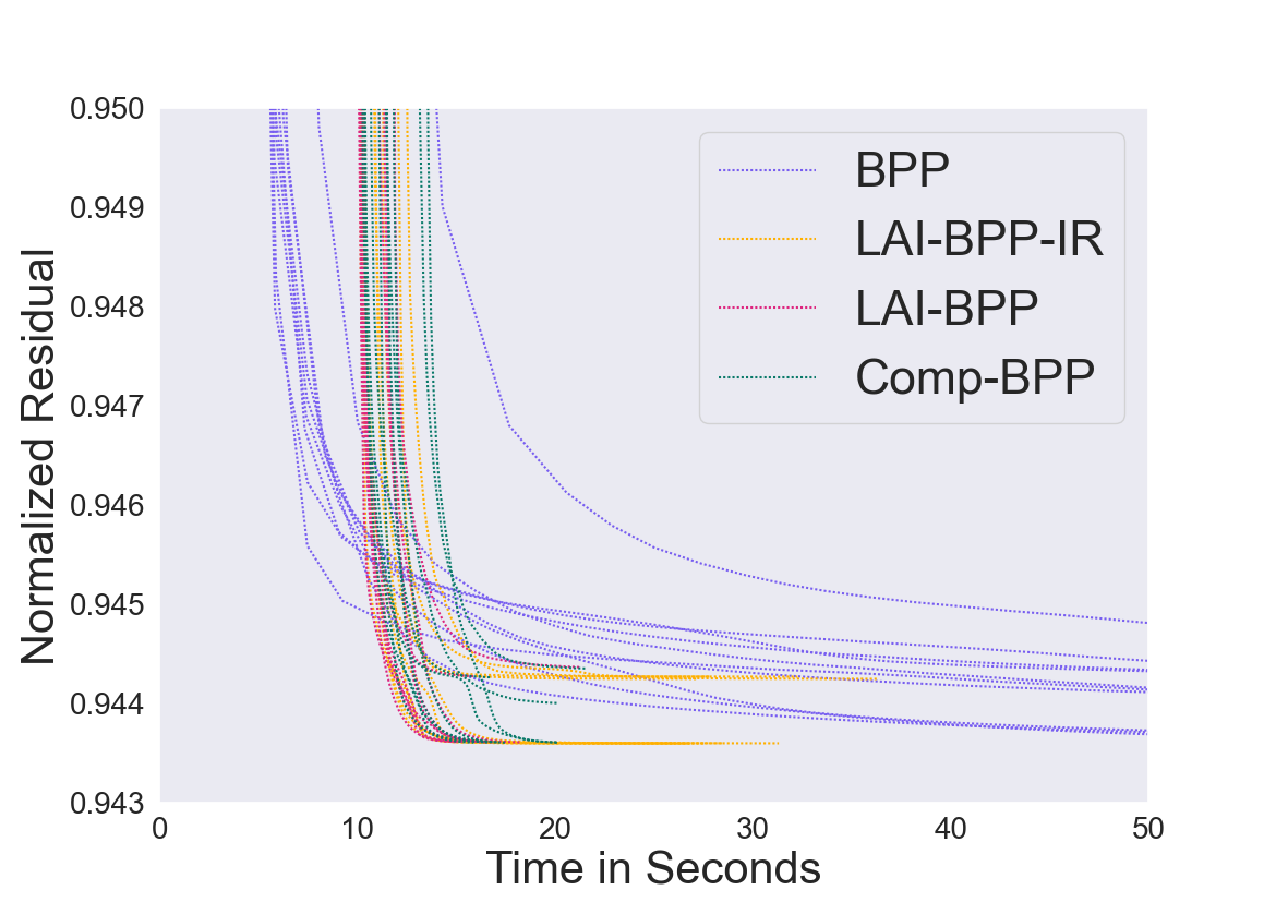
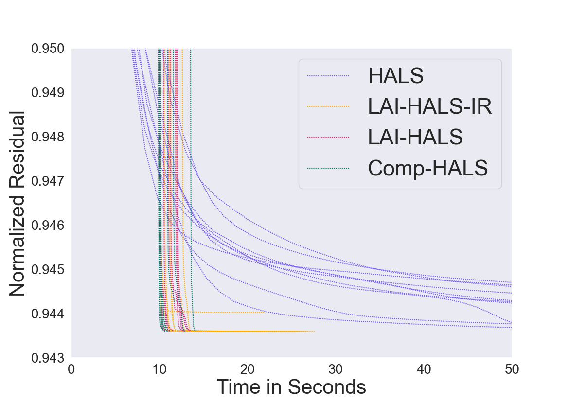
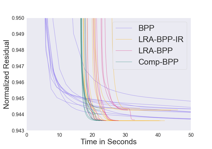
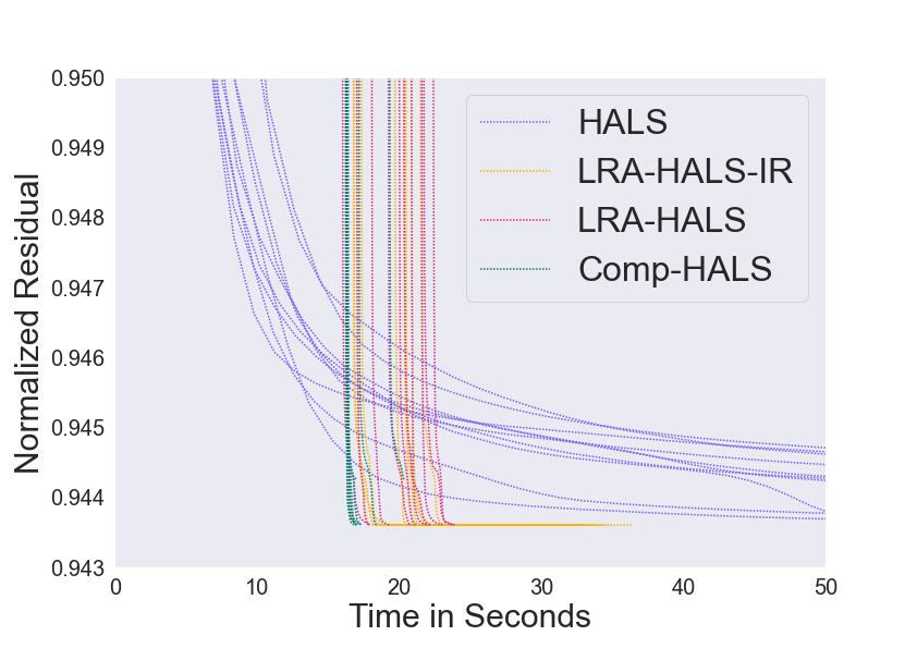
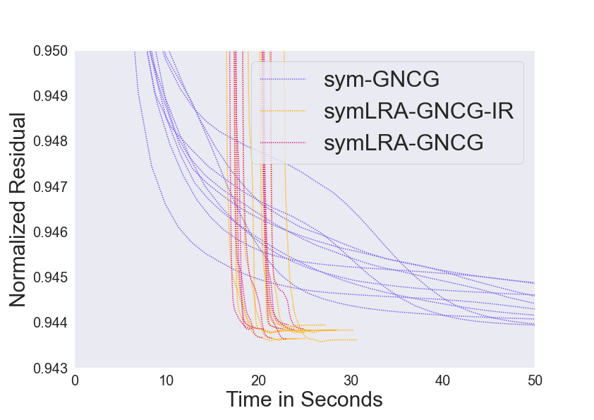
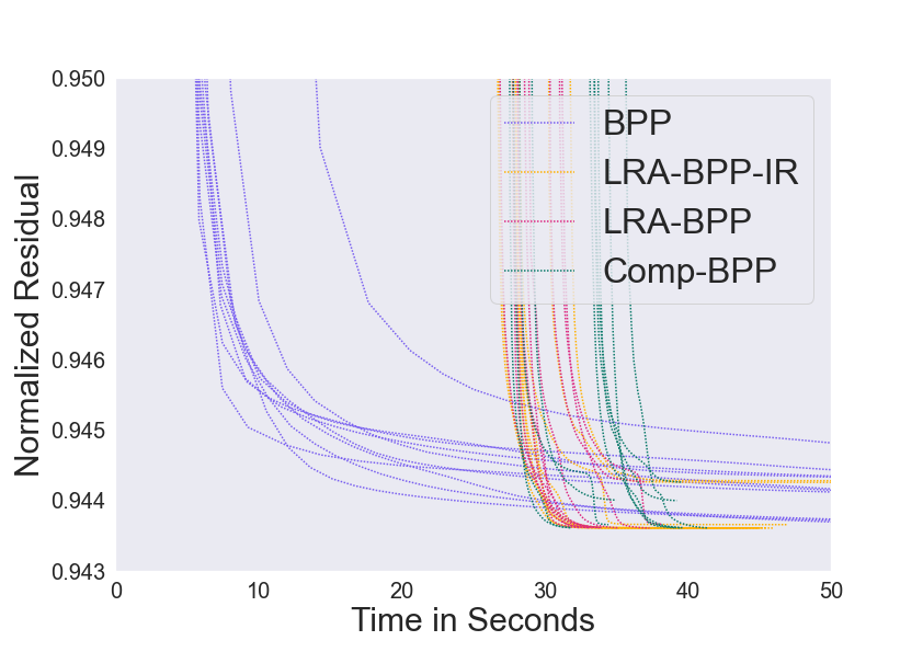
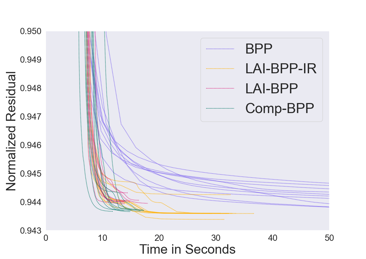
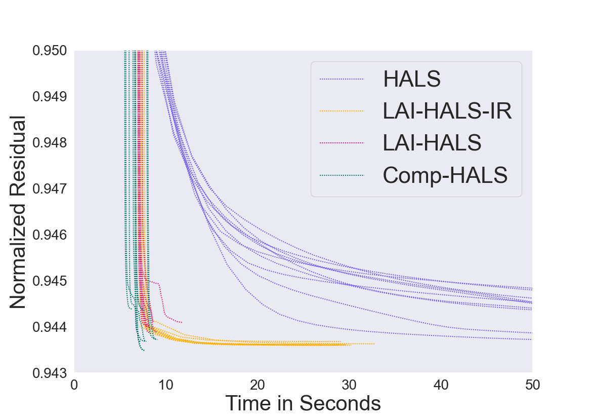
The convergence results for these experiments are shown in Figure4.
These show that the LAI-SymNMF method results in significant speed up. LAI-SymNMF without Iterative Refinement (IR) achieves about a 4 speed up over standard SymNMF with BPP.
For LAI-SymNMF with HALS we observe a speed up of 7.5.
For both BPP and HALS, IR does not appear to be needed when Ada-RRF finds a good starting low-rank approximation.
For comparison we include the SymNMF variant of the “Compressed NMF” method, from [41], and see that it performs nearly identically to LAI-SymNMF.
See SectionA.2 for a discussion of the similarity of the two methods.
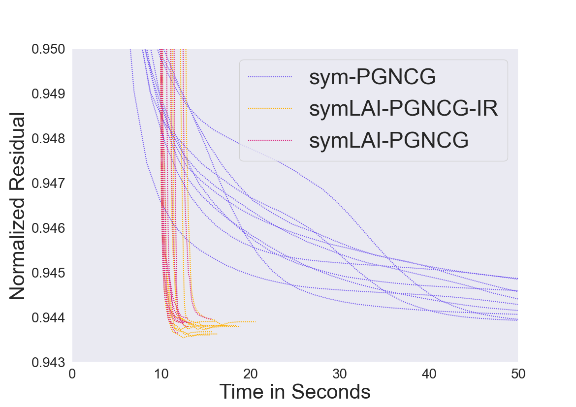
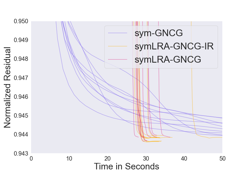
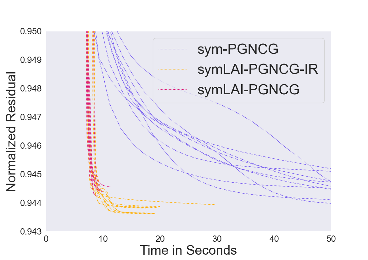
In terms of the PGNCG method in Figure4(c) and Table2 we see that randomization greatly benefits PGNCG resulting in about a speed up.
Additionally, IR in conjunction with PGNCG achieves the lowest normalized residual norm.
Overall we see that randomized methods for SymNMF result in significant speed up while preserving, or even improving, solution quality.
Note that we do not report results for LvS-SymNMF on this data set as the code took prohibitively long to execute.
Plots showing the projected gradient values for each algorithm can be found in SectionC.2.
We include this metric as it is often used as an alternative stopping criteria for NMF and its variants [23, 13].
Plots and tables showing results for different values of the oversampling parameter are also provided.
We find that varying does not have much effect on the solution quality but can negatively impact run time.
Finally, SectionC.2 includes plots and tables showing that the use of AlgorithmAda-RRF provides better overall results than using a static choice of with IR.
We briefly compare against Spectral Clustering as described in [35, 19]
to validate SymNMF-based clustering results.
Spectral clustering achieves an average ARI of over 20 runs.
This is a worse ARI score than all of the SymNMF methods we try, see Table2.
We also note that the normalized residual achieved by a rank SVD is .
(a)BPP
(b)HALS
(c)PGNCG
Figure 1: Normalized Residual Norm Plots for the WoS data set. Three different update rules are shown: BPP, HALS, and PGNCG.
Alg.
Iters
Time
Avg. Min-Res
Min-Res
Mean-ARI
PGNCG
50.8
80.311
0.944
0.9437
0.3063
LIA-PGNCG
92.1
12.834
0.9439
0.9437
0.3107
PGNCG-IR
93.8
16.984
0.9437
0.9435
0.3161
BPP
38.1
66.95
0.9439
0.9436
0.3224
LIA-BPP
71.5
16.734
0.9438
0.9436
0.3264
LIA-BPP-IR
79.0
29.062
0.9439
0.9436
0.3148
Comp-BPP
79.3
18.266
0.9438
0.9436
0.3207
HALS
58.1
92.461
0.9437
0.9436
0.3201
LIA-HALS
97.0
12.124
0.9436
0.9436
0.3269
LIA-HALS-IR
90.5
23.799
0.9436
0.9436
0.3205
Comp-HALS
75.0
11.454
0.9437
0.9436
0.3237
Table 2: Metrics for the various run shown in fig.4. Iters is mean number of iterations taken, Tim is mean run time in seconds, Avg. Min-Res is average minimum achieved residual, Min-res is overall lowest achieved residual, and Mean-ARI is the mean ARI score. Averages are taken over 20 runs.
5.2 Microsoft Open Academic Graph
We run our methods for SymNMF on the Microsoft Open Academic Graph (OAG) [47].
This is a data set that combines the Microsoft Academic Graph (MAG) [39] and the Arnet-Miner (Aminer) academic graph [40].
From the OAG333https://github.com/ramkikannan/planc we take a subset of 37,732,477 papers and use their citation information to form a sparse graph with 966,206,008 non-zeros as in [14].
This adjacency matrix is symmetrically normalized and the diagonal is zeroed out following the methodology in [25].
The rank is set to for all experiments.
The parameter is set to where is the dimension of the square input matrix.
The regularized version of SymNMF in Equation3 requires an input hyperparamter to balance the two objectives.
Of course the sampled problem will also need this hyperparameter.
We propose that using the same values of for the leverage score sampling method and the deterministic method is reasonable since and .
AlgorithmLvS-SymNMF is run with BPP and HALS as the update rules.
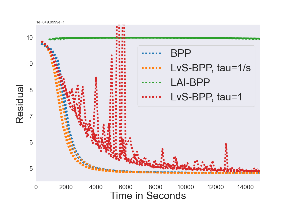
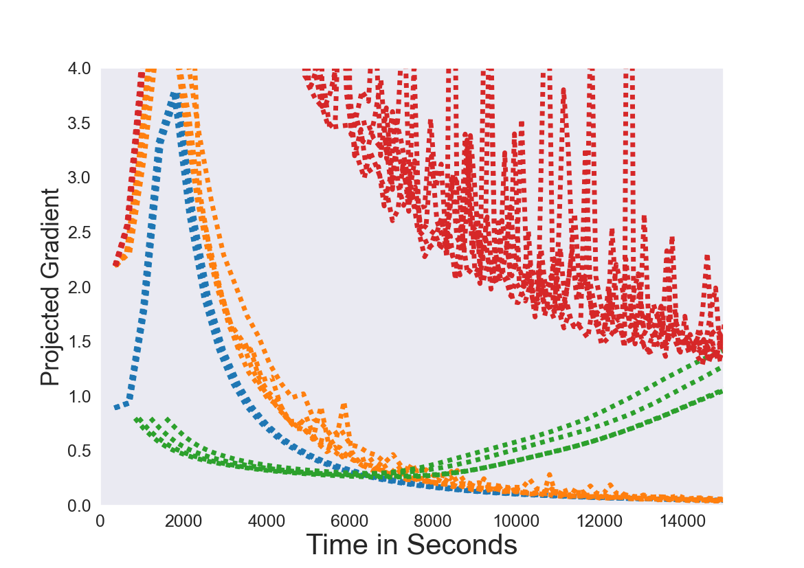
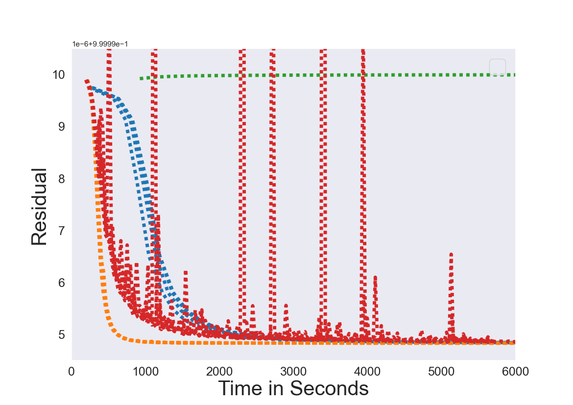
The normalized residual norms and the projected gradient values are shown in Figure2.
First we note that the LAI method with BPP update rule is generally unsuccessful at reducing the error.
We hypothesize that this is because the RRF produces a LAI with a large value of as in Equation15.
Next we note that using the Hybrid Sampling method is important to achieve good speed-up.
In the case of the BPP update rule, in Figure2(a) one can observe that the purely random method () does not provide any speed up over the standard BPP method.
However when the hybrid method with is used one can see that the leverage score sampling algorithm becomes competitive.
When the BPP update rule is used, a significant amount of the time per iteration goes into solving the NLS problems.
So while leverage score sampling effectively eliminates the cost of multiplying by , only about a speed up is achieved as leverage score sampling has no effect on the cost of the update function. In the case of HALS, we observe significantly better speed up when leverage score sampling is used.
Figure2(a) clearly shows that hybrid leverage score sampling outperforms both leverage score sampling and the standard HALS method.
The hybrid leverage score sampling method in this case is able to achieve about a speed up per iteration over standard HALS.
We note that the use of our new HALS update rules, as in Equations5 and 6, is crucial for obtaining good performance.
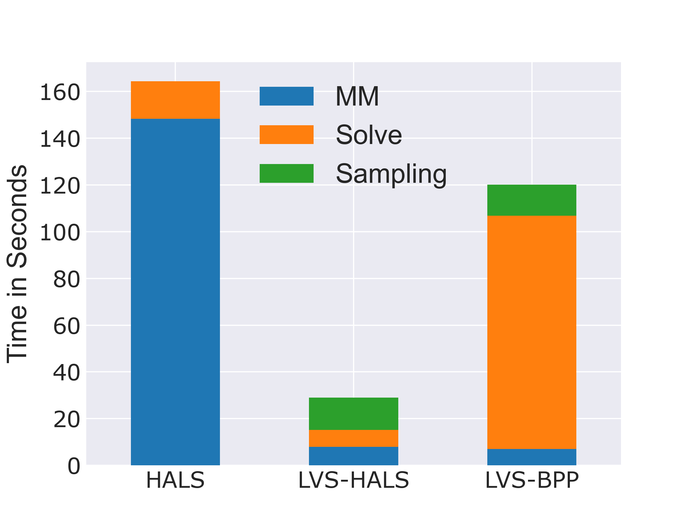
Figure3 shows the time break down for 3 algorithms: leverage score sampling with HALS and BPP as the update rule and a standard NMF method with HALS as the update rule.
The timings are divided into 3 categories: 1) “Matrix Multiplication” (MM) for computing the four main matrix products, 2) “Solve” for the time spent in the update rule (e.g. time spent in the BPP solver), and 3) “Sampling” time spent performing leverage score sampling which includes computing the thin QR decomposition.
We can see that the MM time is greatly reduced by using leverage score sampling while incurring an acceptable overhead in terms of sampling time.
Lastly we see that this data confirms that the BPP solver is limiting potential computational gains from leverage score sampling.
(a)BPP, Normalized Residual Value
(b)BPP, Projected Gradient Value
(c)HALS, Normalized Residual Value
(d)HALS, Projected Gradient Value
Figure 2: Normalized residual and projected gradient values for OAG using HALS and BPP update rules. , .Figure 3: Time Breakdown per iteration for three algorithms. Standard SymNMF with HALS update rule (HALS), SymNMF with leverage score sampling and HALS (LvS-HALS), and SymNMF with leverage score sampling and BPP (LvS-BPP).
5.2.1 Results for the OAG
We now analyze the output of running the LvS-SymNMF algorithms on the OAG.
The factors with are used to form clusters, as in the experiment before on the WoS hypergraph, following the methodology in [25].
Since this data set does not come with ground truth, assessing the quality of the LvS-SymNMF outputs is more difficult.
The residuals output by both the HALS and the LvS-HALS method differ by a tiny amount, on the order of 1e-12, with the leverage score method achieving the lower residual.
The two sets of clusters produced by the methods are different, as can be immediately deduced from the difference in cluster sizes.
Standard HALS produces one huge cluster containing all but around of the vertices.
These vertices are then split into an additional 15 clusters whose sizes range from around 5000 to 8000 vertices.
The LvS-HALS method finds 3 large clusters of sizes about million, million, and .
The remaining 13 clusters have between one to six thousand vertices each.
Cluster-0 is the largest cluster for both methods.
Cluster-15 and Cluster-10 are the million and thousand sized cluster for LVS-HALS.
The smaller clusters are all somewhat connected to Cluster-0 and sparsely, if at all, connected to each other.
To analyze these clusters more rigorously we compute the Silhouette Scores for each vertex [37].
For a set of clusters for we define the following quantities for a vertex in cluster
Here measures a vertex’s similarity to its own cluster, measures a vertex’s similarity to the next most similar cluster and is the graph adjacency matrix input to the algorithm SymNMF.
The Silhouette Score for is then given by
Silhouette Scores range from to , with meaning a vertex is very similar to its own cluster and meaning it should be moved to its next closest cluster.
Individual vertex scores are then averaged over their cluster memberships to obtain cluster level Silhouette Scores.
Note that this definition of Silhouette Score is for similarity metrics and so is slightly different that the typical Silhouette Score equation which is defined for dissimilarity metrics.
The Silhouette Scores are computed for each cluster.
The Silhouette Scores for the HALS methods are perfect with the exception of Cluster-0, which still achieves a high score of 0.78.
The Silhouette Scores for the LVS-HALS algorithm are not as high as the ones for HALS but are still well above 0.
The exception is Cluster-0 (from LVS-HALS), which has a near 0 Silhouette Score of , meaning that it does not form a good cluster but also that its vertices do not necessarily belong in one of the other clusters.
Other than Cluster-0 the LVS-HALS method finds clusters with mean Silhouette Score ( Standard Deviation).
This indicates that the LVS-HALS method is able to find well structured clusters in terms of Silhouette Score.
To further validate that LVS-HALS is finding meaningful clusters we show the top 10 words associated with Clusters 10 to 15 in Table3.
More data about this experiment can be found in SectionD.2.
T10
T11
T12
T13
T14
T15 \csvreader[head to column names]CSV_Data/pdT_lvs_twords.csv
\topicP
Table 3: Top key words for Leverage Score HALS output. Topics 10-15 from the Microsoft Open Academic Graph run using HALS as the update rule with Leverage Score sampling () and . The 10 top key words in terms of tf-idf association are shown in the table. We can see many of the top key words per topic seem to form a coherent subject matter.
6 Conclusion
We have presented two novel algorithms for computing SymNMF in a randomized way.
These methods are suitable for large problems as demonstrated by our findings on two data sets.
Comparing these two methods we believe that the AlgorithmLAI-SymNMF method is appropriate when a high quality LAI can be computed quickly and captures the underlying NMF signal.
In other cases AlgorithmLvS-SymNMF can be used.
Our proposed methods achieve significant speeds ups of 5 or more and produce quality solutions on downstream clustering tasks.
Additionally our techniques are applicable to standard NMF formulations as well.
Finally we presented a number of theoretical results that justify why and when our proposed algorithms perform well in practice.
These results include an analysis of leverage score sampling for approximately solving Nonnegative Least Squares problems, sample complexity analysis for the Hybrid Sampling scheme from [27], and some guarantees for AlgorithmLAI-SymNMF.
Appendix A Additional Material for LAI-SymNMF
A.1 Additional Material and Reference for LAI-NMF Theory
LAI-SymNMF is similar to the randomized NMF algorithms proposed in [13, 41].
The “Randomized HALS” method proposed in [13] which destroys symmetry is inherently unsymmetric, as it compresses only one dimension of the matrix, and so we do not consider comparing against it.
In fact LAI-SymNMF could be viewed as a natural extension of this “Randomized HALS” method to randomized SymNMF.
The so called “Compressed-NMF” algorithm proposed in [41] can be straightforwardly extended to the SymNMF problem.
We do so and compare against it later.
Generally, Compressed-NMF operates as follows: 1) compute two approximate orthonormal bases for and as and respectively and
2) alternatingly solve the two problems
The products and can be computed once but and need be recomputed each iteration.
In this way a smaller problem is solved at each iteration resulting in computational savings.
This method can be used for SymNMF by applying it to Equation3.
Additionally, in the symmetric case one need call the RRF only once.
We relate Compressed-NMF to LAI-NMF in the following way.
Consider a QB-decomposition computed using the RRF where and .
Using the decomposition for LAI-NMF in Equation12, the update to and its Quadratic Program (QP) form are
Taking the QP formulation for the Compressed NMF update for ,
, yields
The term on the right, , is the same for both problems.
The difference between the two methods comes from the fact that the Gram matrix in LAI-NMF is but the Gram in Compressed-NMF contains the projection .
Empirically, for SymNMF, we find that these methods perform nearly identically.
From this perspective we argue the affect of in the Gram matrix is minimal.
Overall we propose that the LAI approach is easier to reason about, as it simply fits an NMF model of the low-rank approximation of .
As previously stated, using the basis as a sketch for NLS problems is not justified theoretically.
A.3 Low-rank Approximate Input Projected Gauss-Newton with Conjugate Gradients for SymNMF
This section contains the pseudo code for the PGNCG method with low-rank approximate inputs.
The original algorithm was developed for high performance distributed computing environments [15].
The Pseudocode is given in AlgorithmLAI-PGNCG-SymNMF.
The only alterations to this pseudo code are lines 3 and 7.
This highlights how simple the idea of LAI-SymNMF is in practice.
[H]
Algorithm LAI-PGNCG-SymNMF : SymNMF of a Low-Rank Approximation
1:input: a symmetric matrix , target rank , column oversampling parameter , power iteration exponent , and max number of CG iterations
2: as the factors for an approximate rank- SymNMF of .
3:function LAI-SymNMF()
4:
5: [ Apx-EVD(), % Obtain approximate basis for range of , and
6: Initialize
7:while Convergence Crit. Not Met do
8:
9: This replaces
10:
11:
12:fordo
13:
14:
15:
16:
17:
18:
19:endfor
20:
21:endwhile
22:endfunction
Appendix B Derivation of Symmetrically Regularized HALS
This section presents the derivation of the regularized HALS method for SymNMF and its efficient updating.
For this derivation is symmetric throughout.
Define
Where is without the th column and similar for .
Then the rank one update equation can be posed as
Next denote the matrix and the vector as (Note that we have flipped sign here)
Now apply the standard HALS update
Finally the efficient updating method is derived as
The final update rule is written as
for the columns of and this can be done similarly for the columns of .
Appendix C Stopping Criteria
Having a stopping criteria is often useful for NMF algorithms.
In this work we use two measures the Normalized Residual and the Projected Gradient to measure convergence.
C.1 Residual Checks
The NMF algorithms often require computation of the residual or the normalized residual
(29)
However, checking the residual working with the full matrix can be computationally expensive.
Since checking the residual requires working with the full data matrix it can potentially dominate the run time of a randomized algorithm.
Therefore, it is important to have an appropriate method for estimating the residual at each iteration [26, 1].
Residual Computation for LAI-NMF
For LAI-SymNMF the issue is easily remedied as we can simply check the residual against the factored form of as
(30)
This allows for rapid evaluation of an approximate residual using techniques similar to that used for NMF.
Our experiments show this is often a reasonable approach to use.
C.2 Projected Gradients
The norm of the projected gradient is often used as a stopping criteria for NMF algorithms in place of the residual.
The idea is that when the NMF objective is at a stationary point, according to the Karush-Kuhn-Tucker (KKT) conditions, the projected gradients with respect to and will be 0.
Therefore we assume that if the projected gradients are small then we are close to a stationary point.
The projected gradient norm is defined as
(31)
where the partial gradients are
(32)
(33)
and the projected gradient is
(34)
similar for the partial gradient with respect to .
One issue with using the projected gradient as a comparison measure between algorithms is that different diagonal scalings of and can give different projected gradient values [23, 24].
However this is not an issue with the SymNMF objective.
The gradient of Equation2 is given by
(35)
Appendix D Additional Experimental Data
D.1 World of Science Data Set
This section contains some additional experiments on the World of Science data set. The first set of experiments are concerned with varying the or the column over sampling parameter in the RRF.
The observation here is that increasing does not seem to have a beneficial impact on clustering quality or final residual.
Figure4 shows the runs for the various algorithms with and .
Table4 and Table5 give various metrics associated with these runs.
Each algorithm was run 20 times.
“Iters” is average number of iterations, “Time” is the average time in seconds, “Avg. Min-Res” is the average minimum residual achieved, “Min-Res” is the overall minimum residual achieved, and “Mean-ARI” is the mean of the ARI scores for each algorithm.
(a)BPP, p=40
(b)HALS, p=40
(c)GNCG, p=40
(d)BPP, p=80
(e)HALS, p=80
(f)GNCG, p=80
Figure 4: Normalized Residual error value for various SymNMF Algorithms on the WoS data set using a EDVW Hypergraph Representation.
Alg.
Iters
Time
Avg. Min-Res
Min-Res
Mean-ARI \csvreader[head to column names]CSV_Data/WoS_exp31_T.csv
\MeanARI
Table 4: Data Table for the WoS data set. Each algorithm was run 10 times. For LIA methods auto- and . The columns record average number of iterations until the stopping criteria is met, average time in seconds, average minimum residual, and minimum residual achieved over all runs.
Alg.
Iters
Time
Avg. Min-Res
Min-Res
Mean-ARI \csvreader[head to column names]CSV_Data/WoS_exp32_T.csv
\MeanARI
Table 5: Data Table for the WoS data set. Each algorithm was run 10 times. For LIA methods auto- and . The columns record average number of iterations until the stopping criteria is met, average time in seconds, average minimum residual, and minimum residual achieved over all runs.
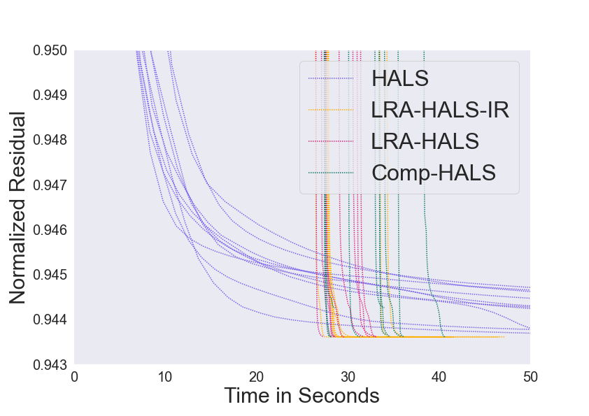
The second set of experiments are run with and without the use of AlgorithmAda-RRF.
Table6 gives data for this run.
One can observe that method without IR do not achieve high quality residual or ARI scores.
While IR can help fix these issues it does so at a higher computational cost.
The convergence plots for these experiments are in Figures5(c), 5(a) and 5(b).
(a)BPP
(b)HALS
(c)PGNCG
Figure 5: Normalized Residual Norm Plots for the WoS data set. Three different update rules are shown: BPP, HALS, and PGNCG. These experiments use and do not make use of AlgorithmAda-RRF.
Alg.
Iters
Time
Avg. Min-Res
Min-Res
Mean-ARI \csvreader[head to column names]CSV_Data/WoS_all_exp25_T.csv
\MeanARI
Table 6: Data Table for the WoS data set. Each algorithm was run 10 times. For LIA methods , no AlgorithmAda-RRF is used. The columns record average number of iterations until the stopping criteria is met, average time in seconds, average minimum residual, and minimum residual achieved over all runs.
WoS Experiments System Details
The WoS experiments were run on a MacBook Pro with MATLAB 2021a.
The MacBook Pro has a 2.3 GHz Quad-Core Intel Core i7 processor and 16 GBs of RAM.
MATLAB was given access to all 4 cores.
D.2 Microsoft Open Academic Graph Experiments
This section contains additional data related to the Microsoft OAG experiments.
Table7 shows the top 10 words for each cluster found by the HALS algorithm and Table8 shows the top 10 words for each cluster found by the LVS-HALS algorithm.
System Details
Experiments on the OAG dataset were run on the Hive Cluster at the Georgia Institute of Technology.
The runs were given access to eight Xeon 6226 CPU @ 2.70GHz on a single shared memory node.
Experiments were run in MATLAB version 2019a.
Topic
TW1
TW2
TW3
TW4
TW5
TW6
TW7
TW8
TW9
TW10 \csvreader[head to column names]CSV_Data/pd_hals_twords.csv
\twordsJ
Table 7: Top key words for HALS output. Run on the Microsoft Open Academic Graph.
Topic
TW1
TW2
TW3
TW4
TW5
TW6
TW7
TW8
TW9
TW10 \csvreader[head to column names]CSV_Data/pd_lvs_twords.csv
\twordsJ
Table 8: Topwords for Leverage Score HALS output. Selected topics from the Microsoft Open Academic Graph run using HALS as the update rule with Leverage Score sampling (). The 10 top words in terms of tf-idf association are shown in the table. We can see many of the top key words per topic seem to form a coherent subject matter.
Appendix E Fast Residual Evaluation in NMF
The NMF residual is given by .
This quantity can be computed cheaply by reusing already computed quantities from the previous update.
To see this observe that
The need only be computed one time, computing is cheap as long as and can reuse the most recent Gram matrix (either or ), and can be computed cheaply by reusing the more recently computed product with depending on the update order of and .
This method can easily be used with LAI-SymNMF to compute at each iteration.
Therefore we are able to evaluate the residual for almost free at each iteration of the algorithm.
This is important for determining when to stop iterating.
Appendix F Adaptive Randomized Range Finder
Using the standard “trick” for efficiently checking the residual we can derive the following formula which we use in AlgorithmAda-RRF :
To the check the residual of our LAI we need only compute the matrix .
This can then be used in the next power iteration if needed.
Algorithm Ada-RRF Adaptive Randomized Range Finder
1:input: data matrix , target rank , oversampling parameter , maximum number of power iterations
2:
3:function Apx-EVD()
4:
5: Draw a Gaussian Random matrix
6: Compute
7:whiledo
8:
9: Evaluate
10:
11:if Stopping Criteria satisfied then
12: break
13:endif
14:
15:
16:endwhile
17: Return
18:endfunction
Appendix G Update() Function
In this section we thoroughly explain the Update() function we use to simplify our pseudocode.
The Framework for Alternating Updating NMF (FAUN) was proposed for the design of a massively parallel NMF code [21].
In the FAUN the matrix products , , , and are computed and used to perform updates.
Many of the most effective NMF update rules require the computation of these 4 matrices as they appear in the gradient of the NMF NLS subproblems
(36)
and
(37)
Many methods can be implemented using the FAUN.
We now briefly discuss a few of the more popular methods.
Multiplicative Updates
is one of the most popular methods for performing NMF updates. Proposed in [29], it is guaranteed to non increase the objective function and uses the rules
Hierarchical Least Squares
(HALS) uses the following update rules
All the columns of and are updated in sequence.
This method is popular for its good convergence properties and its simplicity to implement.
Alternating Nonnegative Least Squares
ANLS updates the full and matrices in an alternating fashion by computing the optimal solutions for the NLS problems Eqns. (37) and (36).
These NLS problems are equivalent to solving the following quadratic programs (QPs)
for every row vector and of and , respectively.
It is simple to see that all of these rules rely on the aforementioned four matrix products.
Our proposed algorithms LAI-SymNMF and LvS-SymNMF can use any of these updates rules, and more e.g. projected gradient methods for solving NLS problems [30].
Appendix H Theorems for Randomized Numerical Linear Algebra
This section contains a number of theorems that we use from the Randomized NLA literature.
H.1 Structural Condition Theorems
We include statements of the two Structural Conditions taken from the work by Larsen and Kolda [27].
These theorems are included for completeness and reference.
Teorema 7.
Given consider its SVD and its row leverage scores for each row , where denotes the set of integers form 1 to .
Let be an overestimate of the leverage score such that for some it holds that for all , where denotes the probability corresponding to the th leverage score.
Construct a row sampling and rescaling matrix via importance sampling according to the leverage score overestimates .
If then the following equation holds with at least probability
for all and .
This theorem tells us that all the singular values of are close to 1 if we take enough samples .
Note that this implies
(38)
H.2 Randomized Matrix Multiply
Teorema 8.
Consider two matrices and and their product .
Construct a sampling matrix with rows that are chosen according to the probability distribution with a such that for all .
Define as vector of length of sampled indices such that is the index of the th sampled row.
Consider the approximate matrix product
Then the approximate matrix product satisfies
Applying Theorem (8) in conjunction with Markov’s Inequality we obtain the following Lemma
Lemma 9.
Taking samples where results in
being true with probability .
Proof.
Applying Markov’s Inequality we have
So if it is desired that this hold with probability then .
∎
H.3 Matrix Chernoff Bounds
This is a Matrix Chernoff Bound taken from [45] which is used to show the validity of the Hybrid Sampling leverage scores matrix.
Teorema 10.
Matrix Chernoff Bound:
Let be independent copies of a symmetric random matrix with , , and .
Let .
Then for any we have
(39)
H.4 Frobenius Norm Deviation Bound for the Randomized Range Finder
This section contains a partial statement of Theorem 5.8 from [17].
Teorema 11.
Let be a low-rank approximationg of , with , obtained from the RRF with desired low-rank , power iteration parameter , column over sampling parameter and a parameter .
Define
.
Then with probability the following holds:
References
[1]
Casey Battaglino, Grey Ballard, and Tamara G. Kolda.
A practical randomized cp tensor decomposition.
SIAM Journal on Matrix Analysis and Applications,
39(2):876–901, 2018.
[2]
C. Boutsidis and E. Gallopoulos.
Svd based initialization: A head start for nonnegative matrix
factorization.
Pattern Recognition, 41(4):1350–1362, 2008.
[3]
Christos Boutsidis and Petros Drineas.
Random projections for the nonnegative least-squares problem.
Linear Algebra and its Applications, 431(5):760–771, 2009.
[4]
Dehua Cheng, Richard Peng, Yan Liu, and Ioakeim Perros.
Spals: Fast alternating least squares via implicit leverage scores
sampling.
In D. Lee, M. Sugiyama, U. Luxburg, I. Guyon, and R. Garnett,
editors, Advances in Neural Information Processing Systems, volume 29.
Curran Associates, Inc., 2016.
[5]
Dongjin Choi, Barry Drake, and Haesun Park.
Co-embedding multi-type data for information fusion and visual
analytics.
In 2023 26th International Conference on Information Fusion
(FUSION), pages 1–8, 2023.
[6]
Dongjin Choi, Andy Xiang, Ozgur Ozturk, Deep Shrestha, Barry Drake, Hamid
Haidarian, Faizan Javed, and Haesun Park.
Wellfactor: Patient profiling using integrative embedding of
healthcare data.
arXiv preprint arXiv:2312.14129, 2023.
[7]
James W. Daniel.
Stability of the solution of definite quadratic programs.
Mathematical Programming, 5, 1973.
[8]
Petros Drineas, Malik Magdon-Ismail, Michael W. Mahoney, and David P.
Woodruff.
Fast approximation of matrix coherence and statistical leverage.
CoRR, abs/1109.3843, 2011.
[9]
Petros Drineas, Michael W. Mahoney, S. Muthukrishnan, and Tamás
Sarlós.
Faster least squares approximation.
CoRR, abs/0710.1435, 2007.
[10]
Rundong Du, Barry Drake, and Haesun Park.
Hybrid clustering based on content and connection structure using
joint nonnegative matrix factorization.
Journal of Global Optimization, 74:1 – 17, 08 2019.
[11]
Rundong Du, Da Kuang, Barry Drake, and Haesun Park.
Dc-nmf: nonnegative matrix factorization based on divide-and-conquer
for fast clustering and topic modeling.
Journal of Global Optimization, 68(4):777–798, 08 2017.
Copyright - Journal of Global Optimization is a copyright of
Springer, 2017; Last updated - 2023-11-27.
[12]
Rundong Du, Da Kuang, Barry Drake, and Haesun Park.
Hierarchical community detection via rank-2 symmetric nonnegative
matrix factorization.
Computational Social Networks, 4:1 – 26, 09 2017.
[13]
N. Benjamin Erichson, Ariana Mendible, Sophie Wihlborn, and J. Nathan Kutz.
Randomized nonnegative matrix factorization.
Pattern Recognition Letters, 104:1–7, mar 2018.
[14]
Srinivas Eswar, Benjamin Cobb, Koby Hayashi, Ramakrishnan Kannan, Grey Ballard,
Richard Vuduc, and Haesun Park.
Distributed-memory parallel jointnmf.
In Proceedings of the 37th International Conference on
Supercomputing, ICS ’23, page 301–312, New York, NY, USA, 2023.
Association for Computing Machinery.
[15]
Srinivas Eswar, Koby Hayashi, Grey Ballard, Ramakrishnan Kannan, Richard Vuduc,
and Haesun Park.
Distributed-memory parallel symmetric nonnegative matrix
factorization.
In SC20: International Conference for High Performance
Computing, Networking, Storage and Analysis, pages 1–14, 2020.
[16]
Nicolas Gillis.
Nonnegative Matrix Factorization.
Society for Industrial and Applied Mathematics, Philadelphia, PA,
2020.
[17]
M. Gu.
Subspace iteration randomization and singular value problems.
SIAM Journal on Scientific Computing, 37(3):A1139–A1173, 2015.
[18]
Nathan Halko, Per-Gunnar Martinsson, and Joel A. Tropp.
Finding structure with randomness: Probabilistic algorithms for
constructing approximate matrix decompositions.
2009.
[19]
Koby Hayashi, Sinan G. Aksoy, Cheong Hee Park, and Haesun Park.
Hypergraph random walks, laplacians, and clustering.
In Proceedings of the 29th ACM International Conference on
Information & Knowledge Management, CIKM ’20, page 495–504, New York, NY,
USA, 2020. Association for Computing Machinery.
[20]
Liangshao Hou, Delin Chu, and Li-Zhi Liao.
A progressive hierarchical alternating least squares method for
symmetric nonnegative matrix factorization.
IEEE Transactions on Pattern Analysis and Machine Intelligence,
45(5):5355–5369, 2023.
[21]
Ramakrishnan Kannan, Grey Ballard, and Haesun Park.
A high-performance parallel algorithm for nonnegative matrix
factorization.
In Proceedings of the 21st ACM SIGPLAN Symposium on Principles
and Practice of Parallel Programming, PPoPP ’16, New York, NY, USA, 2016.
Association for Computing Machinery.
[22]
Hannah Kim, Jaegul Choo, Jingu Kim, Chandan K. Reddy, and Haesun Park.
Simultaneous discovery of common and discriminative topics via joint
nonnegative matrix factorization.
In Proceedings of the 21th ACM SIGKDD International Conference
on Knowledge Discovery and Data Mining, KDD ’15, page 567–576, New York,
NY, USA, 2015. Association for Computing Machinery.
[23]
Jingu Kim, Yunlong He, and Haesun Park.
Algorithms for nonnegative matrix and tensor factorizations: A
unified view based on block coordinate descent framework.
J. of Global Optimization, 58(2):285–319, feb 2014.
[24]
Jingu Kim and Haesun Park.
Fast nonnegative matrix factorization: An active-set-like method and
comparisons.
SIAM Journal on Scientific Computing, 33(6):3261–3281, 2011.
[25]
Da Kuang, Sangwoon Yun, and Haesun Park.
Symnmf: Nonnegative low-rank approximation of a similarity matrix for
graph clustering.
Journal of Global Optimization, 62, 07 2015.
[26]
Brett W. Larsen and Tamara G. Kolda.
Practical leverage-based sampling for low-rank tensor decomposition,
2020.
[27]
Brett W. Larsen and Tamara G. Kolda.
Sketching matrix least squares via leverage scores estimates, 2022.
[28]
Daniel Lee and H. Seung.
Learning the parts of objects by non-negative matrix factorization.
Nature, 401:788–91, 11 1999.
[29]
Daniel Lee and H. Sebastian Seung.
Algorithms for non-negative matrix factorization.
In T. Leen, T. Dietterich, and V. Tresp, editors, Advances in
Neural Information Processing Systems, volume 13. MIT Press, 2000.
[31]
Malik Magdon-Ismail.
Row sampling for matrix algorithms via a non-commutative bernstein
bound.
ArXiv, abs/1008.0587, 2010.
[32]
Michael W. Mahoney.
Randomized algorithms for matrices and data.
CoRR, abs/1104.5557, 2011.
[33]
Michael W. Mahoney.
Lecture notes on randomized linear algebra.
CoRR, abs/1608.04481, 2016.
[34]
Per-Gunnar Martinsson and Joel Tropp.
Randomized numerical linear algebra: Foundations & algorithms, 02
2020.
[35]
Andrew Y. Ng, Michael I. Jordan, and Yair Weiss.
On spectral clustering: Analysis and an algorithm.
In Proceedings of the 14th International Conference on Neural
Information Processing Systems: Natural and Synthetic, NIPS’01, page
849–856, Cambridge, MA, USA, 2001. MIT Press.
[36]
Dimitris Papailiopoulos, Anastasios Kyrillidis, and Christos Boutsidis.
Provable deterministic leverage score sampling.
In Proceedings of the 20th ACM SIGKDD International Conference
on Knowledge Discovery and Data Mining, KDD ’14, page 997–1006, New York,
NY, USA, 2014. Association for Computing Machinery.
[37]
Peter Rousseeuw.
Rousseeuw, p.j.: Silhouettes: A graphical aid to the interpretation
and validation of cluster analysis. comput. appl. math. 20, 53-65.
Journal of Computational and Applied Mathematics, 20:53–65, 11
1987.
[38]
Tamas Sarlos.
Improved approximation algorithms for large matrices via random
projections.
In 2006 47th Annual IEEE Symposium on Foundations of Computer
Science (FOCS’06), pages 143–152, 2006.
[39]
Arnab Sinha, Zhihong Shen, Yang Song, Hao Ma, Darrin Eide, Bo-June (Paul) Hsu,
and Kuansan Wang.
An overview of microsoft academic service (mas) and applications.
In Proceedings of the 24th International Conference on World
Wide Web, WWW ’15 Companion, page 243–246, New York, NY, USA, 2015.
Association for Computing Machinery.
[40]
Jie Tang, Jing Zhang, Limin Yao, Juanzi Li, Li Zhang, and Zhong Su.
Arnetminer: Extraction and mining of academic social networks.
In Proceedings of the 14th ACM SIGKDD International Conference
on Knowledge Discovery and Data Mining, KDD ’08, page 990–998, New York,
NY, USA, 2008. Association for Computing Machinery.
[41]
Mariano Tepper and Guillermo Sapiro.
Compressed nonnegative matrix factorization is fast and accurate.
IEEE Transactions on Signal Processing, 64(9):2269–2283, 2016.
[42]
Arnaud Vandaele, Nicolas Gillis, Qi Lei, Kai Zhong, and Inderjit S. Dhillon.
Efficient and non-convex coordinate descent for symmetric nonnegative
matrix factorization.
IEEE Transactions on Signal Processing, 64, 2016.
[43]
Fei Wang and Ping Li.
Efficient nonnegative matrix factorization with random projections.
In SDM, 2010.
[44]
Joyce Jiyoung Whang, Rundong Du, Sangwon Jung, Geon Lee, Barry Drake, Qingqing
Liu, Seonggoo Kang, and Haesun Park.
Mega: Multi-view semi-supervised clustering of hypergraphs.
Proc. VLDB Endow., 13(5):698–711, jan 2020.
[45]
David P. Woodruff.
Sketching as a tool for numerical linear algebra.
CoRR, abs/1411.4357, 2014.
[46]
Wei Xu, Xin Liu, and Yihong Gong.
Document clustering based on non-negative matrix factorization.
In Proceedings of the 26th Annual International ACM SIGIR
Conference on Research and Development in Informaion Retrieval, SIGIR ’03,
page 267–273, New York, NY, USA, 2003. Association for Computing Machinery.
[47]
Fanjin Zhang, Xiao Liu, Jie Tang, Yuxiao Dong, Peiran Yao, Jie Zhang, Xiaotao
Gu, Yan Wang, Bin Shao, Rui Li, and Kuansan Wang.
Oag: Toward linking large-scale heterogeneous entity graphs.
In ACM SIGKDD International Conference on Knowledge Discovery
and Data Mining (KDD), August 2019.
[48]
Guoxu Zhou, Andrzej Cichocki, and Shengli Xie.
Fast nonnegative matrix/tensor factorization based on low-rank
approximation.
IEEE Transactions on Signal Processing, 60(6):2928–2940, 2012.
[49]
Zhihui Zhu, Xiao Li, Kai Liu, and Qiuwei Li.
Dropping symmetry for fast symmetric nonnegative matrix
factorization.
In Proceedings of the 32nd International Conference on Neural
Information Processing Systems, NIPS’18, page 5160–5170, Red Hook, NY,
USA, 2018. Curran Associates Inc.