Anisotropic molecular photoemission dynamics: Interpreting and accounting for the nuclear motion

Abstract

We investigate how vibration affects molecular photoemission dynamics, through simulations on two-dimension asymmetric model molecules including the electronic and nuclear motions in a fully correlated way. We show that a slight anisotropy in the electron-ion momentum sharing is sufficient to prevent one from unambigously characterizing the vibrationnaly averaged photoemission dynamics in terms of stereo Wigner delays. We further show that vibrational resolution can be retrieved in fixed-nuclei simulations, using effective molecular conformations that are specific to each vibrational channel. The optimal internuclear distances found empirically in 1-photon processes can be identified a priori using simple physical arguments. They also turn out to be efficient to simulate vibrationnally-resolved RABBIT measurements and to account for interchannel coherences in broadband 1-photon ionization.

I Introduction

From its early emergence as an applied branch of attosecond sciences to its most recent and ongoing developments, attochemistry offers and envisions unprecedented ways of exploring fundamental dynamics occurring in molecules on their natural time scale [1, 2, 3, 4, 5, 6, 7]. In the broader perspective of attosecond time-resolved spectroscopies, photoemission endorses a singular role, either as a characterization tool [8, 9] or as the probed process itself [10, 11, 12].

Revisiting a process as essential as molecular photoemission in the time domain is made possible only through intertwined, long term interactions between theory and experiments, that tackle and exploit the complexities and richness specific to molecular systems both in the conception and in the interpretation of simulations or measurements. It was pioneered by investigating experimentally the intricate dynamics of resonant ionization in N₂ with vibrational resolution [13], using the ‘reconstruction of attosecond beatings by interferences of two-photon transitions’ (RABBIT) scheme [8, 14]. The interpretation of the measured channel-selective RABBIT phases in terms of transition delays was subsequently clarified by means of simulations on low-dimensional model molecules [15, 16]. The experimental results were furthermore reproduced and expanded recently in elaborate simulations aiming at a quantitative agreement [17]. The anisotropy of ionization dynamics, which is another essential feature of molecular photoemission, was considered first in simulations of attosecond ‘streaking’ measurements [9, 18] on a model CO molecule [19] and then explored experimentally, also on CO, using RABBIT [20]. Further experimental and theoretical investigations addressing anisotropy have since then been reported on systems of increasing complexities [21, 22, 23, 24, 25, 26], see also [27] and references therein.

The imprints of nuclear motion on photemission dynamics in polyatomic molecules is the subject of an increasing number of theoretical and experimental investigations. Among the most recent studies, the authors of Ref. [28] investigate theoretically how nuclear motion affects photoelectron spectra in the context of RABBIT measurements. In this context, they establish an expression of molecular RABBIT spectra in terms of a convolution between a nuclear autocorrelation function and two-photon electronic transition matrix elements, following an approach initially derived to simulate molecular streaking [29]. In [30], the imprints of nuclear motion on attosecond photoemission delays is investigated experimentally on the methane molecule and its deutered counterpart, using RABBIT and an advanced theoretical support. The authors find no significant isotopic effect, but a $\sim 20$ as difference between dissociative and non-dissociative channels. A closely related study on the same polyatomic molecules further highlighted how nuclear motion impacts the coherence of the photoemission process [31], which is an essential issue for most of the interferometric attosecond resolved pump-probe schemes.

Nonetheless, investigations on smaller – diatomic – benchmark molecules [32, 33, 34, 35, 36, 37, 38, 39, 40, 41, 42, 43, 44] remain of great importance to gradually and comprehensively explore the interplay of the molecular degrees of freedom from a time-dependent perspective. On the theory side, simulations on simple models with limited degrees of freedom [45] are essential to guide and interpret experiments and elaborate simulations in terms of intuitive pictures and practical notions.

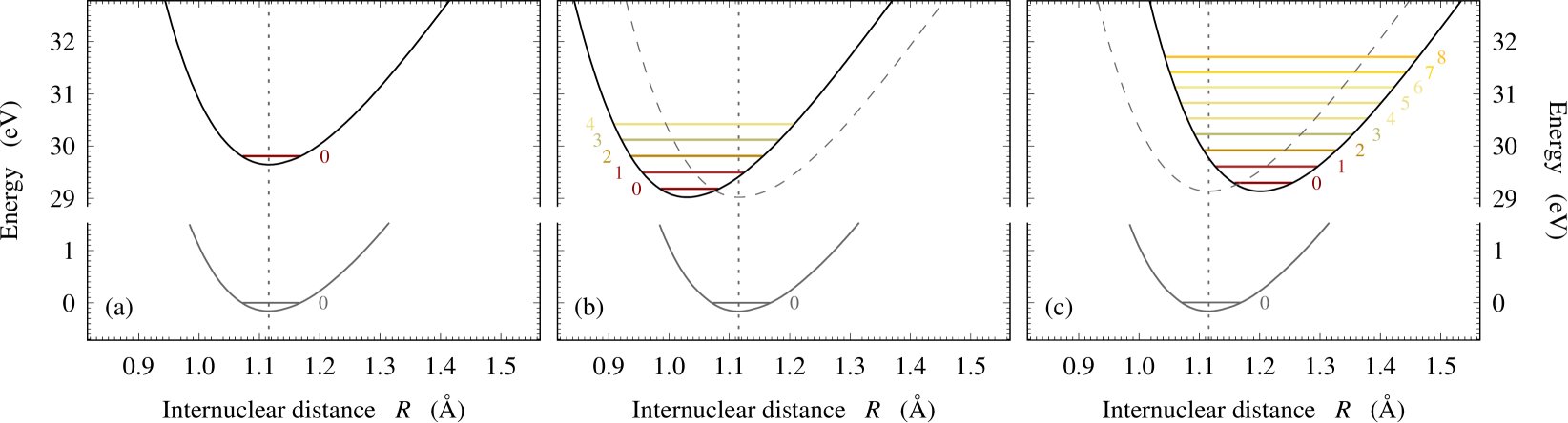
Figure 1: (Color online) Born-Oppenheimer energies of the model molecules $\mathcal{A}$ [frame (a)], $\mathcal{B}$ [frame (b)] and $\mathcal{C}$ [frame (c)] designed for the simulations, as a function of the internuclear distance $R$. The energy scale refers here to the overall ground states of the neutral molecules. For each molecule, the full grey and black curves correspond to the neutral and ionic electronic ground states, respectively. In frames (b) and (c), the dashed grey curve is an image of the neutral ground curve vertically shifted towards the ionization threshold, displayed for comparison purpose. The vertical dotted lines indicate the equilibrium distance of the neutral $R_{\text{\tiny eq}}$. The vibrational levels $v$ presenting a significant overlap with the ground state [$|F(v)|^{2}>10^{-2}$, see Eq. (21) and Fig. 7] are indicated in the ionic curve of each molecule .

In the present article, we investigate numerically how vibration imprints the attosecond dynamics of anisotropic molecular photoemission even when the vibronic couplings are minimal – notably far from any vibronic resonance. Our study is based on low dimensional model molecules allowing for extensive numerically exact simulations. The objectives are two-fold: i) to study the interplay of molecular asymmetry and nuclear motion on attosecond time-resolved photoemission, and ii) to identify a way to account for the vibrational resolution in standard theoretical approaches with fixed nuclei – keeping in mind that only the latter can be routinely applied to the simulations of more realistic models.

The paper is organized as follows. Section II presents the model molecules and the overall methodology followed in our study. In section III, we benchmark the signatures of molecular asymmetry on 1-photon ionization dynamics with a model displaying no effective nuclear motion during and upon photoemission. It partly reproduces and expands the results presented and commented in [27]. In section IV, we consider photoemission occurring with sensible nuclear motion. We question the relevance of defining an orientation-resolved photoemission delay for the photoelectron wave packet averaged over the open vibrationnal channels. Then we consider vibrationnaly-resolved photoemission dynamics, and investigate the possibility to reproduce it in a fixed-nuclei approach. In Section IV.3 we address the capacities of the fixed nuclei approach to reproduce coherent, vibrationnally-resolved, photoemission beyond the context in which it was designed. The conclusions are presented in section V.

Unless stated otherwise, the equations are displayed in atomic units (a.u.) all through the paper.

II Theoretical toolbox

II.1 Model molecules

Our simulations were performed on single-active electron diatomic model molecules including correlated electronic and internuclear motions each in 1D. They are similar to the ones used eg in [46, 47, 15].

II.1.1 Generic hamiltonian

The generic field-free hamiltonian of the model molecules reads

$$H_{0} = \underbrace{-\frac{1}{2\mu}\frac{\partial^{2}}{\partial R^{2}}+V_{\text{\tiny N-N}}(R)}_{H_{\text{\tiny N}}}\underbrace{-\frac{1}{2}\frac{\partial^{2}}{\partial x^{2}}+V_{\text{\tiny N-e}}(x,R)}_{H_{\text{\tiny e}}}$$ (1)

where the two coordinates $x$ and $R$ are the electron position and the internuclear distance, respectively, $\mu$ is the nuclei reduced mass, $V_{\text{\tiny N-N}}(R)$ is the interatomic potential in absence of the active electron, and $V_{\text{\tiny N-e}}(x,R)$ is the interaction potential between the active electron and the molecular ion.

The interatomic potential $V_{\text{\tiny N-N}}$ for each molecule is defined numerically on a discretized $R$-grid, while the electron-nuclei potential $V_{\text{\tiny N-e}}$ is defined as an asymmetric two-center soft-Coulomb potential,

$$V_{\text{\tiny N-e}}(x,R) = \sum\limits_{j=1,2}-\frac{q_{j}}{\sqrt{(x-X_{j})^{2}+a(R)}}$$ (2)

where

$$X_{j} = (-1)^{j}\frac{\mu}{M_{j}}R$$ (3)

are the positions of each nucleus ($j=1,2$), of mass $M_{j}$, with respect to their center of mass. The $V_{\text{\tiny N-e}}$ potential is adjustable through the effective charges $q_{j}>0$ (with the constraint $q_{1}+q_{2}=1$) and the screening parameter $a(R)>0$ defined numerically over the same $R$-grid as $V_{\text{\tiny N-N}}$. One should note that $V_{\text{\tiny N-e}}$ accounts not only for the asymmetry related to the electronegativity difference (through $q_{j}$) but also for the mass asymmetry (through $X_{j}$).

In practice, we adjusted $V_{\text{\tiny N-N}}$ and $V_{\text{\tiny N-e}}$ empirically [45] for the energies of the model molecule to match some desired energy curves within the Born-Oppenheimer (BO) approximation: $V_{\text{\tiny N-N}}$ is directly the molecular ion energy curve, while the negative eigen-energies of $H_{\text{\tiny e}}+V_{\text{\tiny N-N}}$ computed at each $R$ [see partition of $H_{0}$ in Eq. (1)] provide the electronic ground and excited curves of the neutral. Within the BO framework, the ground state energy $\varepsilon_{0}(R)$ of the electronic hamiltonian $H_{\text{\tiny e}}$ is the opposite of the vertical ionization potential for each $R$,

$$\tilde{}E_{\text{{I}}}(R) = -\varepsilon_{0}(R),$$ (4)

i.e., the energy gap between the ionic and the neutral ground state curves.

II.1.2 Model parameters

We considered three model molecules, hereafter referred to as $\mathcal{A}$, $\mathcal{B}$ and $\mathcal{C}$ for simplicity. For each of them, the effective charges were set to $q_{1}=0.33$ a.u. and $q_{2}=0.67$ a.u, and the nuclei masses to $M_{1}=20.53$ u and $M_{2}=7.47$ u. The chosen masses are such that $M_{1}+M_{2}=28$ u, i.e., the mass of CO – a prototypical hereronuclear diatomics on which orientation- and time-resolved photoemission simulations [19] and experiments [20] have already been performed. However, our models are only loosely based on CO, as we, among other liberties, increased the mass ratio $M_{2}/M_{1}$ in order to emphasize the consequences of mass asymmetry on photoemission dynamics. The potentials were adjusted to obtain the BO curves displayed in Fig. 1. The three molecular systems share the same ground state energy curve, which mimics the one of CO [48], with an equilibrium distance $R_{\text{\tiny eq}}=1.115$ Å.

In molecule $\mathcal{A}$, the ionic curve is a vertically shifted image of the ground state. In molecule $\mathcal{B}$ (resp. $\mathcal{C}$), it is also a replica of the ground state curve, translated towards lower (resp. larger) values of $R$ with its minimum at $1.029$ Å (resp. $1.201$ Å). The energy shifts of the ionic curves were adjusted to achieve $\tilde{}E_{\text{{I}}}(R_{\text{\tiny eq}})\simeq 30$ eV for all molecules ($29.81$ eV, $29.18$ eV and $29.30$ eV for molecules $\mathcal{A}$, $\mathcal{B}$ and $\mathcal{C}$, respectively). As an illustration, the $x$-dependency of the electron-core potential for molecule $\mathcal{A}$ at the equilibrium distance $R=R_{\text{\tiny eq}}$ can be found in Fig. 4(a).

Due to the relative positions of these energy curves, photoionization takes place with no effective nuclear motion in molecule $\mathcal{A}$, while it initiates a bond contraction in molecule $\mathcal{B}$ and an elongation in molecule $\mathcal{C}$.

II.2 Methodology overview

We considered two different approaches for the simulations. The first one consists in simulating the ‘complete’ vibronic dynamics of the model molecules. To this end, we performed numerically converged, vibronically correlated, simulations based on the resolution of the time-dependent Schrödinger equation (TDSE). The second approach consists in adopting a standard simplified treatment with fixed nuclei, based on the Born-Oppenheimer (BO) approximation, where the photoemission dynamics are encoded in the continuum solutions of the electronic time-independent Schrödinger equation (TISE).

Our motivation is two-fold. On the one hand, the ‘complete’ vibronic simulations highlight the impact of vibronic couplings on the dynamics of molecular photoemission investigated with attosecond resolution. On the other hand, by confronting these ‘exact’ dynamics to the ones obtained in the BO framework, we assess the relevance of fixed-nuclei approaches to investigate molecular photoemission process (see eg [49, 50, 19, 51, 23, 52]), when the latter are performed with well-chosen molecular conformations. In all the simulations, the $x$ origin was set a priori to coincide with the center of mass of the molecule, consistently with the definition of the $V_{\text{\tiny N-e}}$ potential [see Eqs. (2) and (3)].

The central quantities used in this work to characterize anisotropic photoionization dynamics are orientation-resolved yields and stereo ionization delays, which can be computed indifferently in both approaches.

II.2.1 ‘Complete’ simulations

The complete dynamics of the molecules were simulated by solving numerically the vibronic TDSE

$$i\frac{\partial\Phi(x,R,t)}{\partial t} = [H_{0}+W(t)]\Phi(x,R,t).$$ (5)

Here $\Phi(x,R,t)$ is the propagated vibronic wave-function and $W(t)$ represents the dipole interaction of the molecule with the ionizing pulse, implemented in the velocity gauge. The initial state is the ground vibronic state $\Phi_{0}(x,R)$, obtained by imaginary time propagation, in all the simulations. Numerically exact resolutions of the TDSE [Eq. (5)] were performed using a split operator propagation based on a grid representation of the $x$ coordinate, combined with an expansion over a set of eigenvectors of $H_{\text{\tiny N}}$ for the $R$ coordinate, as detailed in [15, 45]. The vector potentials of the ionizing pulses were assigned $\sin^{2}$ temporal envelops with central photon energies $\omega_{\text{\small xuv}}$ corresponding to harmonics of a Ti:Sapphire laser ($\lambda_{0}=800$ nm, $\omega_{0}=1.55$ eV) in the extreme ultraviolet (XUV). Case specific pulse parameters are indicated further in the text. Simulations on molecule $\mathcal{A}$ were performed by expanding the wave-function on a single vibrationnal state ($v=0$ is the only open channel). For molecules $\mathcal{B}$ and $\mathcal{C}$, the results shown in this paper were obtained by including all vibrational channels up to $v=8$ and $17$, respectively, which safely ensures convergence.

The analysis of these complete time-dependent simulations are mostly based on the outgoing electron flux computed in the asymptotic $x$ region, where the short-range components of $V_{\text{\tiny N-e}}$ (including the vibronic couplings) vanish.

II.2.2 Simulations at fixed internuclear distances

In the BO framework, we treated 1-photon ionization by analyzing electronic continuum wave-functions computed at fixed internuclear distances. Among the solutions of the TISE

$$H_{\text{\tiny e}}\psi_{\varepsilon}(x) = \varepsilon\psi_{\varepsilon}(x)$$ (6)

in the degenerate continuum (at energies $\varepsilon>0$), we worked with the wave-functions specifically selected by 1-photon transitions starting from the ground state, hereafter referred to as SCWF for ‘selected continuum wave-functions’. These real-valued continuum wave-functions are defined unambiguously, and their analysis and interpretation are independant from their definition and computation. The SCWF formalism was introduced in [53] and later used in [37, 27]. Note that the electronic hamiltonian $H_{\text{\tiny e}}$ [as defined in Eq. (1)], its eigenfunctions $\psi_{\varepsilon}(x)$ and eigenvalues $\varepsilon$ depend parametrically on the internuclear distance $R$ – although it does not appear explicitely in Eq. (6) for the sake of readability.

Within this framework, the dynamics of photoemission are encoded in the asymptotic features of the SCWF.

More computational details are provided along with the presentation of the results.

III Photoemission from molecule $\mathcal{A}$: signatures of the potential asymmetry

We present here the results obtained for molecule $\mathcal{A}$, which was designed to benchmark our methodological approach. We first detail the analysis of the time-dependent vibronic simulations, and then verify that the latter are consistent with time-independent BO simulations at equilibrium distance.

III.1 ‘Complete’ simulations

In these simulations, the XUV pulse intensities were set to $10^{12}$ W/cm², i.e., low enough to avoid any significant multi-photon process in 1-color photoionization. The total pulse durations were set to $15.87$ fs, which corresponds to 6 fundamental periods ($T_{0}=2\pi/\omega_{0}=2.67$ fs).

III.1.1 Photoelectron flux

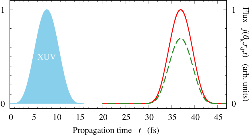
Figure 2: Outgoing electron flux $j(\theta_{\mbox{\tiny k}},r_{\text{\tiny d}},t)$ computed at $r_{\text{\tiny d}}=800$ a.u. on the left ($\theta_{\mbox{\tiny k}}=180\degree$, red full curve) and right ($\theta_{\mbox{\tiny k}}=0\degree$, green dashed curve) sides of molecule $\mathcal{A}$ ionized by a $\omega_{\text{\small xuv}}=35.67$ eV pulse, as a function of propagation time $t$. The flux are normalized to 1 at the overall maximum reached on the left side. The temporal envelop of the ionizing pulse is represented by the blue filled curve.

In the complete time-dependent simulations, we characterized the ionization dynamics through the outgoing photoelectron flux computed at a given detection distance $r_{\text{\tiny d}}$ from the $x$-origin, on either side of the molecule and averaged over $R$:

$$j(\theta_{\mbox{\tiny k}},r_{\text{\tiny d}},t) = \cos\theta_{\mbox{\tiny k}}\times$$

$$\mathfrak{Im}\int\limits_{0}^{\infty}\,\Phi^{\star}(r_{\text{\tiny d}}\cos\theta_{\mbox{\tiny k}},R,t)\Phi^{\prime}(r_{\text{\tiny d}}\cos\theta_{\mbox{\tiny k}},R,t)\,{d}R$$

where $\Phi^{\star}(x,R,t)$ is the complex conjugate of the vibronic wave-function propagated according to Eq. (5), $\Phi^{\prime}(x,R,t)$ its derivative with respect to $x$. Here and all through the paper, $\theta_{\mbox{\tiny k}}$ represents the direction of photoemission, restricted to two discrete values: $\theta_{\mbox{\tiny k}}=0\degree$ (emission towards the right, $x>0$) and $180\degree$ (towards the left, $x<0$).

As an illustration, Figure 2 shows the flux computed at $r_{\text{\tiny d}}=800$ a.u. (423 Å) on the left and right sides of molecule $\mathcal{A}$ ionized by a pulse of central frequency $\omega_{\text{\small xuv}}=23\times\omega_{0}=35.67$ eV. The flux profiles follow the ionizing pulse envelop (also shown), shifted by $\approx 30$ fs, which is consistent with the time needed for a (nearly) free electron with the energy $\omega_{\text{\small xuv}}-\tilde{}E_{\text{{I}}}(R_{\text{\tiny eq}})=5.86$ eV to cover the distance $r_{\text{\tiny d}}$. The flux maximum $\sim 1.5$ times larger on the left side than on the right side is a clear signature of the photoemission anisotropy.

III.1.2 Orientation-resolved yields and delays

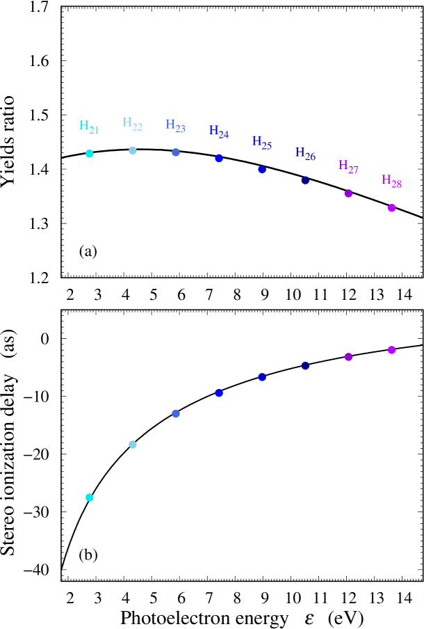
Figure 3: Anisotropic photoemission from molecule $\mathcal{A}$. (a) left/right ionization yields ratio computed in the fully correlated simulations [Eq (9)] and in the BO framework [Eq (14)], resp. $\mathcal{R}$ (circles) and $\tilde{}\mathcal{R}$ (line); (b) stereo ionization delays computed in the fully correlated simulations [Eq (11)] and in the BO framework [Eq (16)], resp. $\Delta\tau$ (circles) and $\Delta\tau_{\mbox{\tiny\sc w}}$ (line). All data plotted as functions of the photoelectron energy $\varepsilon$.

We thus computed the orientation-resolved yields,

$$\mathcal{Y}(\theta_{\mbox{\tiny k}}) = \int\,j(\theta_{\mbox{\tiny k}},r_{\text{\tiny d}},t)\,{d}t,$$ (8)

in a series of simulations with field frequencies corresponding to harmonics 21 to 24, i.e., $\omega_{\text{\small xuv}}$ ranging from $32.57$ eV to $37.23$ eV by $1.55$ eV steps. The corresponding yields ratios

$$\mathcal{R} = \frac{\mathcal{Y}(180\degree)}{\mathcal{Y}(0\degree)}$$ (9)

are displayed in Fig. 3(a) (coloured circles) against the photoelectron energy $\varepsilon$. It evolves smoothly slightly above 1.4, indicating that photoemission is sensitive to the asymmetry of the ionic potential, with little variations over the energy range covered in the simulations.

To characterize the asymmetry of photoemission in the time domain, we used the average “time of flight” (TOF) [15, 53, 16] towards the detector in each direction as

$$\tau(\theta_{\mbox{\tiny k}}) = \frac{\int\limits\,t\times j(\theta_{\mbox{\tiny k}},r_{\text{\tiny d}},t)\,{d}t}{\int\limits\,j(\theta_{\mbox{\tiny k}},r_{\text{\tiny d}},t)\,{d}t}.$$ (10)

To further investigate the angular variations of the TOF computed as such, one must take into consideration the arbitrary origin $x=0$ on either sides of which the virtual detectors are located, and which does not coincide with the average initial position of the electron. In the following, we will therefore characterize these angular variations with the origin-corrected TOF difference,

$$\Delta\tau = \tau(180\degree)-\tau(0\degree)-2\frac{\langle x\rangle_{0}}{\sqrt{2\varepsilon}},$$ (11)

where $\langle x\rangle_{0}$ is the average initial electron position in the ground state of the molecule $\Phi_{0}(x,R)$,

$$\langle x\rangle_{0}=\langle\Phi_{0}|x|\Phi_{0}\rangle.$$ (12)

The role of the last term on the r.h.s of Eq. (11) is discussed in details in the companion paper [27] in the context of time-independent approaches. Its justifications identically holds for time-dependent simulations. It compensates a spurious shift appearing when computing ionization delays with an arbitrary origin – while the photoelectron in average originates from $\langle x\rangle_{0}$. We verified numerically that including this term (after computing the TOFs) is equivalent to shifting the potential such that $\langle x\rangle_{0}=0$ (prior to solving the TDSE). In the present simulations, as well as in molecules $\mathcal{B}$ and $\mathcal{C}$, $\langle x\rangle_{0}=-0.160$ Å.

The stereo ionization delays $\Delta\tau$ obtained for the considered set of XUV frequencies are plotted in Fig. 3(b). Starting from $\sim-40$ as just below $\varepsilon=2$ eV, its magnitude decays smoothly while the photon energy increases, as could be expected in absence of significantly structured continuum. Note that such attosecond delays cannot be resolved visually in Fig. 2, since they are extremely small compared to the temporal spread of the photoelectron wave-packet at detection ($\sim 15$ fs, approximately the XUV pulse duration). They are nonetheless significant and we have ensured their numerical convergence.

Among a series of standard numerical checks, we verified that the measured stereo delays $\Delta\tau$ do not depend on the detection distance $r_{\text{\tiny d}}$ (as long as it lies far enough from the ionic core), which is a fundamental property of the short-range scattering delays.

III.2 Simulations at fixed internuclear distances

Here, we consider the molecule $\mathcal{A}$ at its equilibrium internuclear distance, see Fig. 4(a). It corresponds to the 1D model molecule used for the numerical experiments presented and analysed in [27].

III.2.1 Selected continuum wave-function

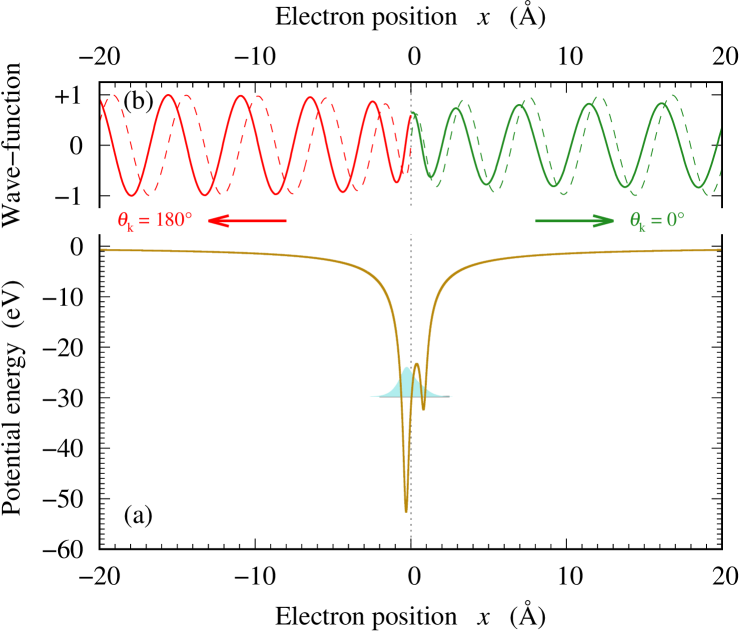
Figure 4: Molecule $\mathcal{A}$ in the BO framework (equilibrium internuclear distance). (a) Electron-nuclei potential $V_{\text{\tiny N-e}}(x,R_{\text{\tiny eq}})$ as a function of the electron position $x$ (dark yellow full curve). The ground state electronic wave-function is also shown (light blue filled curve). (b) Electronic continuum wave-function (full curve) selected at the energy $\varepsilon=5.86$ eV by a 1-photon transition from the electronic ground state. Odd-parity reference wave-function (dashed curve) used to define and compute the orientation-dependent phase-shifts. The displayed continuum wave-functions are normalized such that their amplitudes asymptotically converge to 1 on the left-hand side of the molecule. In this Figure, the left/right discrimination and the parity refer to the arbitrary $x=0$ origin (indicated by a vertical dotted line).

The BO approach relies on the analysis of the electronic continuum wave-functions $\psi_{\varepsilon}(x)$ associated with the photoemission processes. We thus computed the SCWF of molecule $\mathcal{A}$ by solving Eq. (6) over the same energy range as in the full time-dependent simulations, with a fixed internuclear distance set to $R_{\text{\tiny eq}}$.

The SCWF computed at the illustrative energy $\varepsilon=5.86$ eV (corresponding to $\omega_{\text{\small xuv}}=23\times\omega_{0}=35.67$ eV, as in Fig. 2) is shown in Fig. 4(b) (full curve). The pseudo-period of the oscillations on both sides is consistent with a kinetic energy asymptotically converging to $5.86$ eV. Here, the anisotropy of photoemission is clearly visible in the asymmetry of the amplitudes of the SCWF on either sides of the molecule.

III.2.2 Orientation-resolved yields and delays

For each pulse frequency considered in the fully-fledge approach, an alternative evaluation of the orientation-dependent ionization yields is provided, up to a global factor, as

$$\tilde{}\mathcal{Y}(\theta_{\mbox{\tiny k}}) = |A(R_{\text{\tiny eq}};\theta_{\mbox{\tiny k}})|^{2},$$ (13)

where $A(R_{\text{\tiny eq}};,\theta_{\mbox{\tiny k}})$ is the asymptotic amplitude of the SCWF computed with $R=R_{\text{\tiny eq}}$, at the average photoelectron energy, on each side of the molecule. We evaluated these amplitudes using Strömgren’s normalization procedure (see [54] and references therein).

The corresponding yields ratio

$$\tilde{}\mathcal{R} = \frac{\tilde{}\mathcal{Y}(180\degree)}{\tilde{}\mathcal{Y}(0\degree)}$$ (14)

computed over the considered energy range is displayed as a full line in Fig. 3(a). The perfect agreement with the ratio $\mathcal{R}$ computed in the vibronic time-dependent simulations [Eq. (9)] constitutes a first numerical validation of our comparative approach.

From the time domain perspective, we analyzed the SCWF in terms of orientation resolved Wigner delays [55], as detailed in [27]. In few words, the Wigner delay is defined as the spectral derivative

$$\tau_{\mbox{\tiny\sc w}}(\theta_{\mbox{\tiny k}}) = \frac{\partial\eta(\theta_{\mbox{\tiny k}})}{\partial\varepsilon}$$ (15)

of the asymptotic phase shifts of the SCWF computed on each side of the model molecule, with respect to an arbitrary intermediate reference (here, radial Coulomb $s$-waves centered at $x=0$). As explained in [27], and consistently with the ‘complete’ vibronic simulations, we characterized the angular variations of the photoemission dynamics in the BO framework through the origin-corrected stereo Wigner delay

$$\Delta\tau_{\mbox{\tiny\sc w}} = \tau_{\mbox{\tiny\sc w}}(180\degree)-\tau_{\mbox{\tiny\sc w}}(0\degree)-2\frac{\langle x\rangle_{0}}{\sqrt{2\varepsilon}}.$$ (16)

Since the exact ground state of the molecule is accurately modelled by its BO counterpart, the value of the initial average position $\langle x\rangle_{0}$ is the same here as in the ‘complete’ simulations. The stereo Wigner delays computed in the considered energy range, already shown in Fig. 3 of [27], are reported in Fig. 3(b) (full line). They perfectly agree with the stereo delays computed in the ‘complete’ time-dependent simulations.

Apart from benchmarking our comparative approach, the results obtained with molecule $\mathcal{A}$ put forwards the signatures of the left-right electronegativity asymmetry of the molecule on the photoelectron dynamics. The perfect agreement observed in Fig. 3 between the ‘complete’ and the fixed nuclei approach comes as no surprise since (i) the equivalence between the time-dependent and time-independant approaches has already been put forward by Wigner when interpreting in the time-domain the group delay associated with a scattering phase shift [55], and (ii) photoemission of molecule $\mathcal{A}$ occurs with no effective nuclear motion, i.e., the electron and nuclear degrees of freedom, $x$ and $R$, are de facto uncoupled due to the relative positions of the ground state and ionic curves [see Fig. 1(a)].

We now move on to the results obtained with the $\mathcal{B}$ and $\mathcal{C}$ molecules, for which photoemission occurs along with sensible nuclear dynamics.

IV Photoemission from molecules $\mathcal{B}$ and $\mathcal{C}$: signatures of the vibronic couplings

The necessity to take the nuclear motion into consideration in near-threshold photoemission from molecules $\mathcal{B}$ and $\mathcal{C}$ is a consequence of the relative position shifts of their ground states and ionic BO curves [see Fig. 1(b,c)]. We investigate how it affects the photoemission dynamics in the present section by presenting and analyzing the orientation-resolved photoemission yields and stereo delays in these two model molecules, and addressing the relevance of fixed-nuclei simulations in this context.

IV.1 ‘Complete’ simulations

We used here the same pulse parameters as in the simulations with molecule $\mathcal{A}$ (Sec. III.1).

IV.1.1 Signatures of electron-nuclei couplings

A striking signature of the electron-nuclei couplings in the photoemission dynamics of $\mathcal{B}$ shows up in the delays inferred from the outgoing flux. In contrast with the previous case, the stereo delays measured according to Eqs. (10)–(11) strongly depend on the detection distance $r_{\text{\tiny d}}$. This is illustrated in Table 1 with few representative cases. Not only it evidences a rather dramatic dependency of $\Delta\tau$ with respect to $r_{\text{\tiny d}}$, well above the numerical accuracy of the simulations, but it turns out that $\Delta\tau$ monotonically diverges with increasing $r_{\text{\tiny d}}$ (not shown). This tells us that, the delays computed as such are irrelevant for an objective characterization of the ionization dynamics.

Nevertheless their $r_{\text{\tiny d}}$-dependency bear a crucial information: it suggests that the electron wave-packets travel on each side of the molecule with slightly different average velocities. This is the signature of an anisotropic momentum sharing between the nuclei and the active electron during the concerted ionization/contraction of the molecular ion. It involves the nuclear mass asymmetry since the lighter the nucleus, the more the photoelectron is prone to share kinetic energy with it. The principle, which applies to the average velocity, is sketched in Fig. 5. Assuming that only the lighter nucleus (on the left) significantly moves, the photoelectron ends up with a smaller velocity if it exits in the direction of motion of that nucleus (towards the right) than in the other direction.

$\omega_{\text{\small xuv}}$	$r_{\text{\tiny d}}$	$\Delta\tau$
$32.6$ eV	600 a.u.	119 as
	800 a.u.	153 as
$34.1$ eV	800 a.u.	74 as
	1000 a.u.	89 as

Table 1: Stereo delay $\Delta\tau$ computed according to Eq. (11) in molecule $\mathcal{B}$ for an illustrative set of detection distances $r_{\text{\tiny d}}$ and photon frequencies $\omega_{\text{\small xuv}}$.

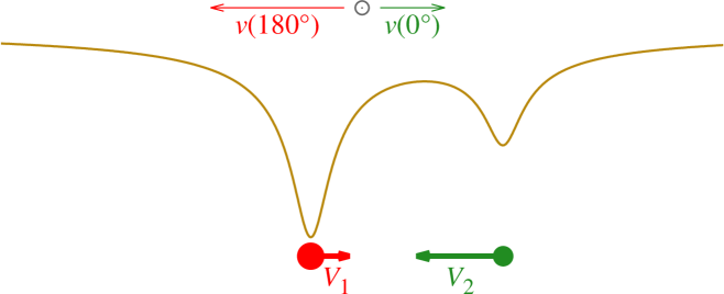
Figure 5: Sketch of the asymmetric average momentum sharing between the photoelectron (empty circle) and the nuclei (full circles) during the photoionization/early contraction of molecule $\mathcal{B}$. For the sake of clarity, the velocity asymmetries have been exagerated compared to the ones obtained in the actual simulations.

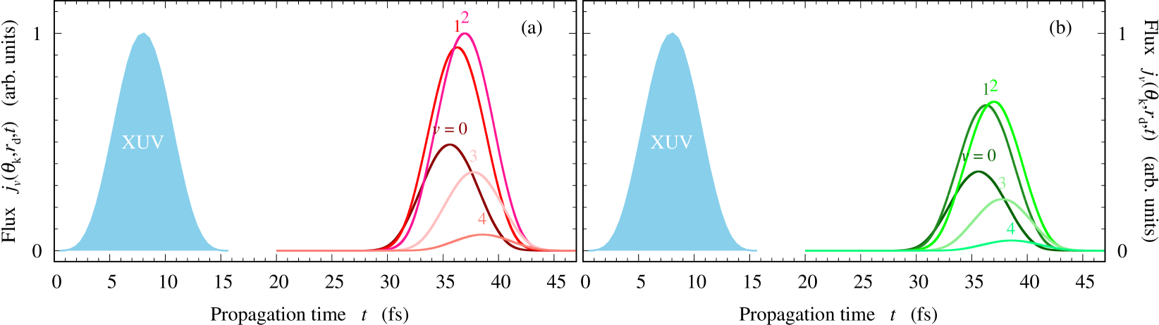
Figure 6: Vibrationally resolved outgoing electron flux $j_{v}(\theta_{\mbox{\tiny k}},r_{\text{\tiny d}},t)$ computed, in the fully correlated simulations, at $r_{\text{\tiny d}}=800$ a.u. on the left [$\theta_{\mbox{\tiny k}}=180\degree$, frame (a)] and right [$\theta_{\mbox{\tiny k}}=0\degree$, frame (b)] sides of molecule $\mathcal{B}$ ionized by $\omega_{\text{\small xuv}}=35.67$ eV pulse, as a function of propagation time $t$, for the 5 first dominant channels. Each curve is labelled according to its corresponding channel ($v=0-4$). The flux are normalized to 1 at the overall maximum reached in the $v=2$ channel, on the left side. The temporal envelop of the ionizing pulse is represented by the blue filled curve.

Properly accounting for this momentum sharing hence requires giving up global characterization and rather considering vibrationnally-resolved observables. In the present context, they are derived from the channel-resolved wave-packets

$$\varphi_{v}(x,t)=\int\limits_{0}^{\infty}\,\chi_{v}(R)\Phi(x,R,t)\,{d}R$$ (17)

in the vibronic TDSE simulations. In Eq. (17), $\chi_{v}(R)$ are the vibrational eigenstates of the molecular ionic core hamiltonian $H_{\text{\tiny N}}$ [see Eq. (1)]. The individual channel functions are relevant as soon as they are uncoupled from each other, i.e., in the asymptotic $x$ region where $V_{\text{\tiny N-e}}$ no longer depends significantly on $R$ (typically beyond few 100 a.u.). Each channel is assigned a specific ionization potential

$$E_{\text{{I}}}(v) = \mathcal{E}^{(+)}_{v}-\mathcal{E}^{(0)}_{0},$$ (18)

where $\mathcal{E}^{(+)}_{v}$ is the energy of the corresponding ionization threshold (in the BO framework, that is the eigenvalue of $H_{\text{\tiny N}}$ associated with $\chi_{v}$) and $\mathcal{E}^{(0)}_{0}$ the vibronic ground energy of the neutral molecule.

The key time-dependent observable becomes the vibrationally-resolved electron flux

$$j_{v}(\theta_{\mbox{\tiny k}},r_{\text{\tiny d}},t) = \cos\theta_{\mbox{\tiny k}}\times$$

$$\mathfrak{Im}\left\{\varphi^{\star}_{v}(r_{\text{\tiny d}}\cos\theta_{\mbox{\tiny k}},t)\varphi^{\prime}_{v}(r_{\text{\tiny d}}\cos\theta_{\mbox{\tiny k}},t)\right\}$$

computed at a distance $r_{\text{\tiny d}}$ on each side of the molecule. Vibrationnally-resolved anisotropic yields and delays can be computed out of the flux $j_{v}(\theta_{\mbox{\tiny k}},r_{\text{\tiny d}},t)$ in a similar fashion than in the integrated case, see Section III.

The flux computed at the distance $r_{\text{\tiny d}}=800$ a.u. on the left (a) and right (b) sides of the $\mathcal{B}$ molecule submitted to a $\omega_{\text{\small xuv}}=35.67$ eV pulse are shown in Fig. 6, for the first few popupated channels. The flux maxima of the different channels are time-shifted from each other, which is a manifestation of the energy conservation law

$$\varepsilon=\omega_{\text{\small xuv}}-E_{\text{{I}}}(v).$$ (20)

The larger $E_{\text{{I}}}(v)$, the lower the photoelectron energy $\varepsilon$ and the larger the time needed to reach the detector. As for molecule $\mathcal{A}$, the asymmetry of molecule $\mathcal{B}$ results in anisotropic ionization yields, visible when comparing the flux magnitudes on the left and on the right. Similar results were obtained with molecule $\mathcal{C}$ (not shown).

To get a better insight on the vibrational distributions upon ionization, we display in Fig. 7, column i, the Franck-Condon (FC) factors for molecules $\mathcal{B}$ (frame a) and $\mathcal{C}$ (frame b), defined as

$$F(v) = \left|\int\limits_{0}^{\infty}\,\chi_{v}(R)\xi_{0}(R)\,{d}R\right|^{2},$$ (21)

where $\xi_{0}(R)$ is the ground vibrational wave-function of the neutral molecule treated in the BO framework. The FC factors peak at $v=1$ for both model molecules, and extend significantly up to $v=4$ and $8$ for molecules $\mathcal{B}$ and $\mathcal{C}$, respectively. They qualitatively reproduce the actual $v$-resolved yields

$$\mathcal{Y}(v;\theta_{\mbox{\tiny k}}) = \int\,j_{v}(\theta_{\mbox{\tiny k}},r_{\text{\tiny d}},t)\,{d}t,$$ (22)

computed on the left (columns ii) and right (columns iii) sides of the molecules ionized by the illustrative $\omega_{\text{\small xuv}}=35.67$ eV pulse. For the sake of comparison, the displayed data are normalized such that each set sums up to 1.

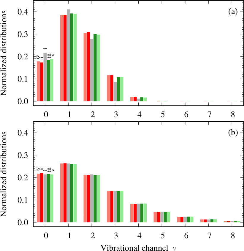
Figure 7: Vibrational distribution of photoemission from molecules $\mathcal{B}$ (a) and $\mathcal{C}$ (b) with a $\omega_{\text{\small xuv}}=35.67$ eV pulse. (i): Franck-Condon factors $F(v)$ [Eq. (21)] ; (ii) and (iii): normalized yields computed in the fully correlated simulations, resp. $\mathcal{Y}(v;180\degree)$ and $\mathcal{Y}(v;0\degree)$ [Eq. (22)]; (iv) and (v): normalized yields computed in the BO framework at the optimal internuclear distances $R_{\text{\tiny opt}}(v)$, resp. $\tilde{}\mathcal{Y}(v;180\degree)$ and $\tilde{}\mathcal{Y}(v;0\degree)$ [Eq. (26)]. The displayed data are normalized such that each set sums up to 1, for comparison purpose.

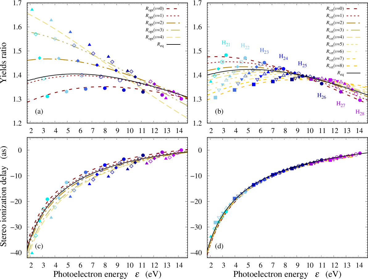
Figure 8: Vibrationnally resolved anisotropic photoemission from molecule $\mathcal{B}$ (left) and $\mathcal{C}$ (right). All data are plotted as functions of the photoelectron energy $\varepsilon$. Left/right yields ratio (top) computed in the fully correlated simulations and in the BO framework, resp. $\mathcal{R}(v)$ (symbols) and $\tilde{}\mathcal{R}(v)$ (lines); stereo delays (bottom) computed in the fully correlated simulations and in the BO framework, resp. $\Delta\tau(v)$ (symbols) and $\Delta\tau_{\mbox{\tiny\sc w}}(v)$ (lines). In all frames, the vibronic data are displayed for the first few significant vibrational channels: $v=0$ (full circles), $1$ (empty circles), $2$ (full diamonds), $3$ (empty diamonds), $4$ (full triangles up), $5$ (empty triangles up), $6$ (full triangles down), $7$ (empty triangles down) and $8$ (full squares). As specified by the inset key, the displayed BO data were computed at a set of $v$-dependent optimal distances [$R_{\text{\tiny opt}}(v)$] for molecule $\mathcal{B}$, and of ‘vertical’ distances [$R_{\text{\tiny vrt}}(v)$] for molecule $\mathcal{C}$ (see text and Tab. 2). The BO data computed at the equilibrium distance ($R_{\text{\tiny eq}}$) are also shown for both molecules.

A feature that cannot be included in the FC factors alone is obviously the orientation dependency. In particular for molecule $\mathcal{B}$, the vibrational distributions of the yields in Fig. 7(a) display slight yet significant differences on the left and right emission sides. In spite of being small, these discrepancies are sufficient to result in different average photoelectron velocities, and to the above-mentioned $r_{\text{\tiny d}}$ dependance of the integrated left-right delay $\Delta\tau$. We emphasize that the data in Fig. 7 are normalized to highlight the orientation-resolved vibrational distributions, and therefore discards the vibrationally-resolved magnitude of the ionization probability on each side of the molecules.

IV.1.2 Photoemission yields and delays

A finer insight on the $v$-resolved photoemission anisotropy is provided in Fig. 8 which shows, for molecules $\mathcal{B}$ [frame (a)] and $\mathcal{C}$ [frame (b)], the yields ratio

$$\mathcal{R}(v) = \frac{\mathcal{Y}(v;180\degree)}{\mathcal{Y}(v;0\degree)}$$ (23)

obtained with several values of $\omega_{\text{\small xuv}}$ in the ‘complete’ simulations (symbols), as a function of the photoelectron energy $\varepsilon$. Their values, comprised between $\sim 1.2$ and $\sim 1.7$, follow for each $v$ the global trend observed with molecule $\mathcal{A}$, see Fig. 3(a). However, they display a clear additional $v$-dependency for both molecules $\mathcal{B}$ and $\mathcal{C}$.

We characterized the dynamics revealed in these simulations consistently with the unresolved case, see Eq. (11). Here, the channel-resolved stereo delays are defined as

$$\Delta\tau(v) = \tau(v;180\degree)-\tau(v;0\degree)-2\frac{\langle x\rangle_{0}}{\sqrt{2\varepsilon}}$$ (24)

where the numerical TOF towards the virtual detector

$$\tau(v;\theta_{\mbox{\tiny k}}) = \frac{\int\limits\,t\times j_{v}(\theta_{\mbox{\tiny k}},r_{\text{\tiny d}},t)\,{d}t}{\int\limits\,j_{v}(\theta_{\mbox{\tiny k}},r_{\text{\tiny d}},t)\,{d}t},$$ (25)

is now computed in each $v$-channel. In Eq. (24), one should keep in mind that $\varepsilon$ implicitly depends on $v$ through Eq. (20), for a given $\omega_{\text{\small xuv}}$. We have notably checked that the vibrationally resolved stereo delays $\Delta\tau(v)$ do not depend on $r_{\text{\tiny d}}$, in contrast with the $v$-integrated data commented before for molecule $\mathcal{B}$ (Table 1). Indeed, for each vibrational channel, energy conservation ensures a symmetric asymptotic electron velocity.

$v$
$E_{\text{{I}}}$ (eV)
$R_{\text{\tiny vrt}}$ (Å)
$R_{\text{\tiny opt}}$ (Å)

(a)
0	1	2	3	4
29.17	29.48	29.78	30.10	30.41
1.076	1.106	1.145	1.201	1.319
1.084	1.113	1.146	1.203	1.248

(b)
0	1	2	3	4	5	6	7	8
29.30	29.61	29.92	30.23	30.53	30.83	31.13	31.42	31.71
1.160	1.135	1.115	1.098	1.082	1.066	1.055	1.041	1.031
1.174	1.148	1.124	1.105	1.091	1.079	1.069	1.055	1.038

Table 2: Channel-dependent ionization energy $E_{\text{{I}}}$ [Eq. (18)] and representative internuclear distances $R_{\text{\tiny vrt}}$ and $R_{\text{\tiny opt}}$ [see text and Eq. (27)] for molecules $\mathcal{B}$ (a) and $\mathcal{C}$ (b) in the main vibrational ionization channels $v$.

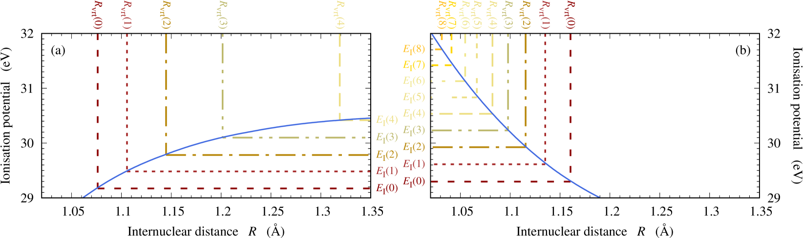
Figure 9: Vertical ionization potential $\tilde{}E_{\text{{I}}}(R)$ of molecules $\mathcal{B}$ (a) and $\mathcal{C}$ (b) as a function of $R$ (blue full curve), used to identify the internuclear distances $R_{\text{\tiny vrt}}(v)$ fulfilling Eq. (27) out of the $v$-dependent ionization potentials $E_{\text{{I}}}(v)$.

The obtained $v$-dependent stereo delays are plotted as symbols in Fig. 8 for molecules $\mathcal{B}$ [frame (c)] and $\mathcal{C}$ [frame (d)]. We first note that they globally behave like the stereo delays reported for molecule $\mathcal{A}$ in Fig. 3(b), with a comparable order of magnitude which decays smoothly towards 0 when the photoelectron energy $\varepsilon$ increases. Besides, a marked $v$-dependency is observed in molecule $\mathcal{B}$, reminiscent of the behavior of the corresponding yields ratios [frame (a)]. In molecule $\mathcal{C}$ however, the values of $\Delta\tau(v)$ appear to depend mostly on $\varepsilon$ regardless of the vibrationnal channel, since all of them follow a common spectral evolution. This is consistent with the normalized vibrational distributions displayed in Fig. 7(b), which are almost identical in the two directions, as pointed out before.

IV.2 Simulations at fixed internuclear distances

In this section, we investigate the possibilities to retrieve the orientation-dependent data, including their $v$-dependencies, by analyzing electronic continuum wave-functions obtained in simulations with fixed nuclei.

The yields ratio and delays computed for both molecules in the BO framework at $R_{\text{\tiny eq}}$ according to Eq. (14) are displayed as a full black lines in Fig. 8. They lie near the data obtained for the dominant channels in the full TDSE simulations (between $v=1$ and $2$), and very close to the equivalent results obtained with $\mathcal{A}$ [see Fig. 3(a)]. Nevertheless, and quite obviously, simulations performed at a single fixed internuclar distance cannot reproduce the non-trivial $v$-dependency observed in the full simulations for the yields ratio and stereo delays of molecule $\mathcal{B}$, and for the yields ratio of molecule $\mathcal{C}$.

Below, we use the simulations performed on molecule $\mathcal{B}$ to identify and interprete $v$-dependent geometries that allow reproducing the results of the vibronic simulations with the fixed nuclei approach. We then assess our interpretation by applying it to fixed nuclei simulations on molecule $\mathcal{C}$.

IV.2.1 Optimal conformations for molecule $\mathcal{B}$

By scanning through the support of the initial vibrational state $\xi_{0}(R)$ of molecule $\mathcal{B}$ ($R\sim 1.0-1.3$ Å), we identified empirically a set of channel-specific optimal distances $R_{\text{\tiny opt}}(v)$ for which both the yields ratio and the stereo delays in the BO approach reproduce the ones of the complete vibronic simulations. The values of $R_{\text{\tiny opt}}(v)$ obtained are reported in Tab. 2(a). The orientation- and channel-resolved yields, now computed in the BO framework at a given optimal conformation for each channel,

$$\tilde{}\mathcal{Y}(v;\theta_{\mbox{\tiny k}}) = |A(R_{\text{\tiny opt}}(v);\theta_{\mbox{\tiny k}})|^{2}\times F(v),$$ (26)

are displayed for the left and right sides in columns iv and v of Fig. 7(a), respectively. They reproduce very well the asymmetric $v$-dependency of the actual yields $\mathcal{Y}(v;\theta_{\mbox{\tiny k}})$ (columns ii and iii). The corresponding yields ratio $\tilde{}\mathcal{R}(v)$ and stereo delays $\Delta\tau_{\mbox{\tiny\sc w}}(v)$, extracted from the SCWF computed at the optimal conformation for each $v$ are displayed as full lines in frames (a) and (c) of Fig. 8. They are in excellent agreement with the $v$-dependent data obtained in the fully correlated simulations for both molecules, apart from the $v=4$, as will be discussed below.

IV.2.2 Physical interpretation

The optimal molecular conformations can be interpreted by looking at the $R$-dependent ionization potential $\tilde{}E_{\text{{I}}}(R)$ [Eq. (4)], which for molecule $\mathcal{B}$ increases monotonically with $R$ within the support of $\xi_{0}(R)$, see Fig. 9(a). On the same figure, we indicate the internuclear distances $R_{\text{\tiny vrt}}(v)$ at which $\tilde{}E_{\text{{I}}}$ matches the $v$-dependent ionization potential [Eq. (18)],

$$\tilde{}E_{\text{{I}}}[R_{\text{\tiny vrt}}(v)] = E_{\text{{I}}}(v).$$ (27)

These “vertical” internuclear distances are reported in Table 2(a), for comparison with the optimal distances found empirically. It turns out that $R_{\text{\tiny opt}}$ matches $R_{\text{\tiny vrt}}$ within $\sim 1\%$ in all the considered channels, except $v=4$ ($\sim 5\%$).

We repeated the same procedure for molecule $\mathcal{C}$. The optimal internuclear distances, $R_{\text{\tiny opt}}(v)$, that we found empirically are reported in Table 2(b), together with the ‘vertical’ ones, $R_{\text{\tiny vrt}}(v)$, extracted from the ionization potential displayed in Fig. 9(b). It is here also a monotonic function of $R$, with opposite variations than for molecule $\mathcal{B}$ (as mentioned earlier, molecule $\mathcal{B}$ expands upon ionization, while molecule $\mathcal{C}$ contracts upon ionization). The BO data displayed as lines in Fig. 8(b) and (d) for molecule $\mathcal{C}$ were directly obtained with $R_{\text{\tiny vrt}}(v)$, for each channel. The differences with the data obtained using $R_{\text{\tiny opt}}(v)$, not shown, would be hardly discernible on that figure. The agreement between the ‘complete’ simulations and the fixed-nuclei approach is here excellent in all considered channels – including the ionization ratios [frame (b)] which follow spectral trends that significantly depend on $v$.

These results provide a simple physical criterion for selecting a priori a set of optimal conformations which allow reproducing, in a fixed-nuclei framework, the details of $v$-dependent molecular photoionization dynamics. It is nevertheless predictable that these specific distances can be representative of the $v$-dependent photoemission dynamics only when $\tilde{}E_{\text{{I}}}(R)$ varies monotonically with $R$. In particular for molecule $\mathcal{B}$ the $\tilde{}E_{\text{{I}}}(R)$ variations are less pronounced as $R$ grows towards the $R_{\text{\tiny vrt}}$ of the highest channels, within the studied range. Consistently, the data computed in the BO framework for molecule $\mathcal{B}$ turned out to be less sensitive to small $R$ variations beyond $R_{\text{\tiny opt}}(v=3)$ – to the extent that we could not find an optimal distance for the $v=4$ channel with the same accuracy as for other channels. This is particularly visible on the yields ratio [Fig. 8(a)], where the BO data never reach the ‘exact’ ones obtained for the highest ($v=4$) channel, the displayed BO data corresponding to $R_{\text{\tiny opt}}(v=4)$ being the closest one could get. This however concerns a minor channel [see Fig. 7(a)]. For molecule $\mathcal{C}$, the narrower dispersions of the data can be directly related to the sharp monotonic decay of $\tilde{}E_{\text{{I}}}$ when $R$ is increased, which implies a narrow dispersion of $R_{\text{\tiny vrt}}(v)$.

IV.3 Illustrative applications of the optimal conformations

In this last section, we address the relevance of the optimal conformations beyond the context in which they were identified. We investigate their relevance first in simulations of interferometric RABBIT measurements, and then to include electron-ion coherences during broadband 1-photon ionization

The RABBIT scheme, together with the attosecond streaking approach, provide indirect ways to access photoemission dynamics, the direct time domain approaches used in our simulations having no experimental equivalent with attosecond resolution (eg magnetic bottles have typical deadtimes of few 10 ns [56] and time-to-digit convertor resolutions in the 100 ps range [57]).

These are interferometric techniques, where the time domain information is extracted from the spectral variations of measured phases. Coherence is thus an essential issue in the design and exploitation of these approaches, the purpose of which is to reveal the fundamental dynamics of essentially quantum processes.

IV.3.1 Intra-channel coherences: RABBIT interferometry

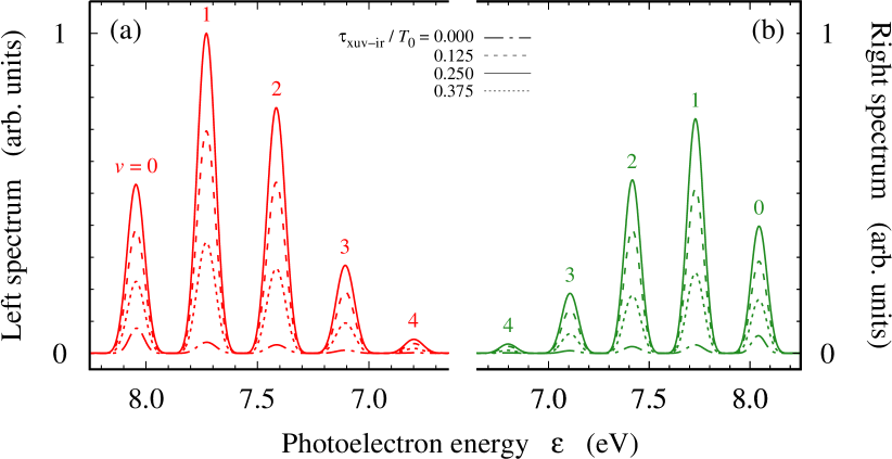
Figure 10: Photoelectron spectra recorded in RABBIT simulations, on the left (a) and right (b) sides of molecule $\mathcal{B}$. The spectral range is focused on sideband 24, and each peak is associated with a specific ionization channel $v=0-4$ (see peak labels). The different spectra were obtained with different values of the pump-probe delay $\tau_{\text{\small xuv-ir}}$ (see inset keys, where $T_{0}=2\times\pi/\omega_{0}$ is the laser period).

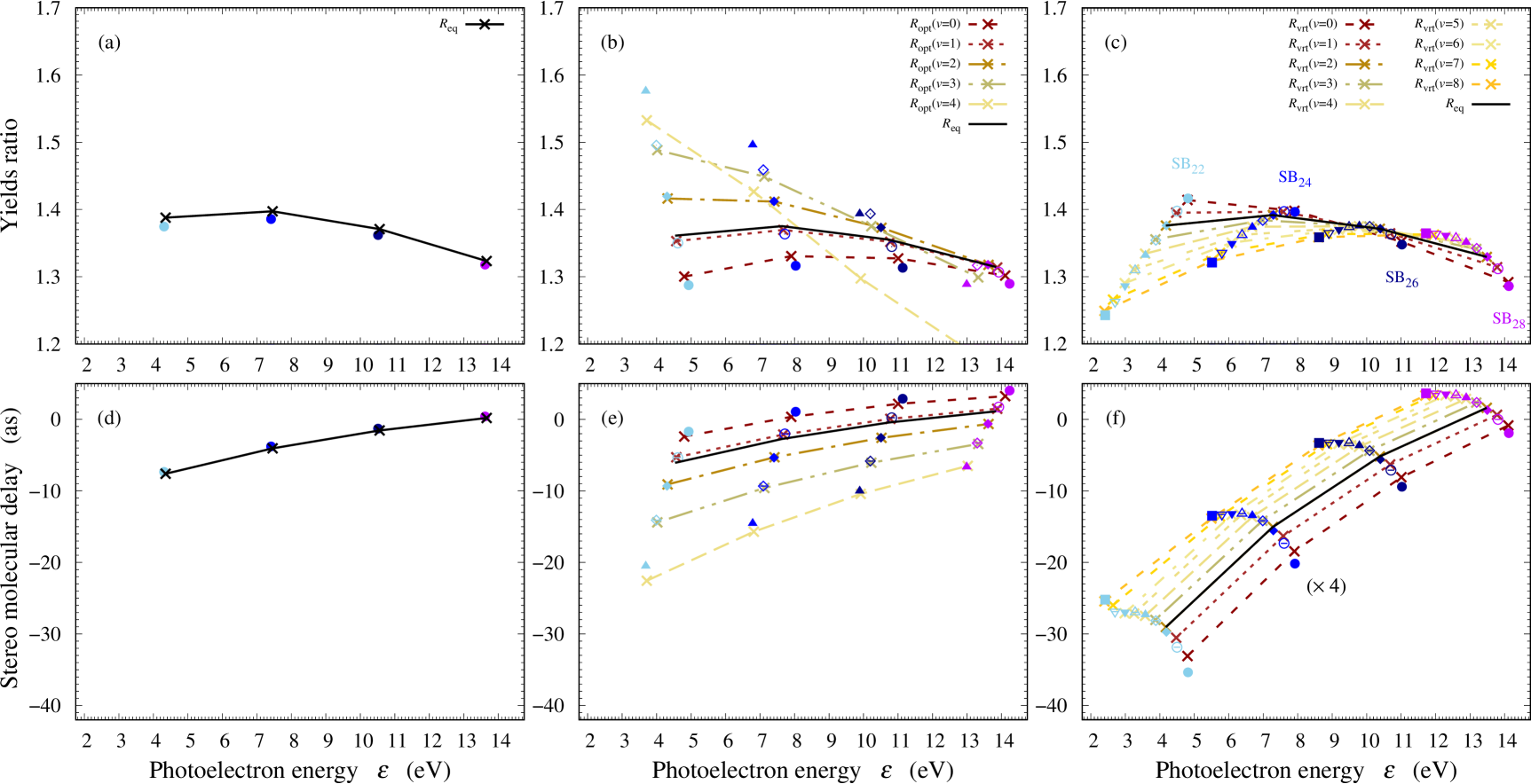
Figure 11: Vibrationnally resolved anisotropic RABBIT simulations in molecule $\mathcal{A}$ (left), $\mathcal{B}$ (center) and $\mathcal{C}$ (right). Data derived from the analysis of sidebands 22 to 28 (right to left) plotted as functions of the photoelectron energy $\varepsilon$. Left-right yields ratio (top) computed in the fully correlated simulations and in the BO framework, resp. $\mathcal{R}_{\text{\tiny rab}}(v)$ (symbols) and $\tilde{\mathcal{R}}_{\text{\tiny rab}}(v)$ (crosses+guidelines); stereo molecular delays (bottom) computed in the fully correlated simulations and in the BO framework, resp. $\Delta\tau_{\mbox{\tiny mol}}(v)$ (symbols) and $\Delta\tilde{\tau}_{\mbox{\tiny mol}}(v)$ (crosses+guideline). In each frame, the data are displayed for the first few significant vibrational channels: $v=0$ (full circles), $1$ (empty circles), $2$ (full diamonds), $3$ (empty diamonds), $4$ (full triangles up), $5$ (empty triangles up), $6$ (full triangles down), $7$ (empty triangles down) and $8$ (full squares). Consistently with the results shown in Fig. 8, the displayed BO data were obtained with the set of $v$-dependent optimal distances [$R_{\text{\tiny opt}}(v)$] identified in 1-photon simulations for molecule $\mathcal{B}$, and of ‘vertical’ distances [$R_{\text{\tiny vrt}}(v)$] for molecule $\mathcal{C}$ (see text and Tab. 2). They were also computed at the equilibrium distance ($R_{\text{\tiny eq}}$) for all molecules. The data displayed in frame (f) are all multiplied by 4 for a better readability.

Following a standard 800-nm RABBIT scheme [8, 14], we simulated photoemission from the three model molecules in presence of the fundamental IR field and a comb of its odd harmonics $\mbox{HA}_{q}$ in the XUV domain (orders $q$ from $21$ to $29$), with an adjustable pump-probe delay $\tau_{\text{\small xuv-ir}}$. We computed vibrationally- and orientation-resolved photoelectron spectra

$$\sigma(v;\varepsilon,\theta_{\mbox{\tiny k}}) = |a(v;\varepsilon,\theta_{\mbox{\tiny k}})|^{2}$$ (28)

out of the final amplitudes corresponding to the ionized molecule, $a(v;\varepsilon,\theta_{\mbox{\tiny k}})$. The latter were obtained in the time-dependent simulations through a position-to-momentum Fourier transform of the channel wave packets $\varphi_{v}(x,t)$ accumulated in the asymptotic region at each time $t$ of the propagation (see Appendix C of [58]).

As expected, we obtained sideband (SB) peaks (orders $22$ to $28$) resulting from 2-photon ${\text{{XUV}}}\pm{\text{{IR}}}$ transitions, the intensities of which oscillate when $\tau_{\text{\small xuv-ir}}$ is tuned [59]. We used long enough pulses (80 fs for the XUV and for the IR) to resolve the vibrational channels in each sideband. This is illustrated in Fig. 10, which shows the vibrationally-structured, orientation and delay-dependent $\mbox{SB}_{24}$ obtained with molecule $\mathcal{B}$. Similarly to the 1-photon case, the relative peak intensities evidence a significantly larger photoemission probability towards the left (a) than towards the right (b). Note however that the orientation-dependency of the SB oscillations are too subtle to be resolved visually in this figure. This is consistent with the ultrashort timescale of the simulated non-resonant photoemission processes [27].

We thus performed a RABBIT analysis consisting in fitting the generic function given in Eq. 8 of [27] to the $\tau_{\text{\small xuv-ir}}$ evolution of each sideband peak associated with a given vibrational channel $v$, and a given direction $\theta_{\mbox{\tiny k}}$. The fitting procedure gives access to the orientation and channel-resolved phases of the peak oscillations $\vartheta(v;\theta_{\mbox{\tiny k}})$, as well as to the $\tau_{\text{\small xuv-ir}}$-averaged photoelectron yields $P(v;\theta_{\mbox{\tiny k}})$. Since the XUV components in our simulations were all synchronized (i.e., they carry no attochirp), $\vartheta(v;\theta_{\mbox{\tiny k}})$ directly corresponds to the so-called “molecular phase”, see [27] and references therein.

We performed simulations both in the fully correlated approach, and in the BO framework. The main results are shown in Fig. 11, for $\mbox{SB}_{22}$ to $\mbox{SB}_{28}$ in molecules $\mathcal{A}$ (left), $\mathcal{B}$ (center) and $\mathcal{C}$ (right). The disconnected symbols in the upper and lower frames respectively correspond to the ratio of the $\tau_{\text{\small xuv-ir}}$-averaged yields,

$$\mathcal{R}_{\text{\tiny rab}}(v) = \frac{P(v;180\degree)}{P(v;0\degree)}$$ (29)

and the “stereo molecular delay” [12, 19]

$$\Delta\tau_{\mbox{\tiny mol}}(v) = \frac{\vartheta(v;180\degree)}{2\times\omega_{0}}-\frac{\vartheta(v;0\degree)}{2\times\omega_{0}}$$ (30)

obtained in the fully correlated approach for the main $v$ channels. As in the 1-photon case, these quantities follow standard general trends which can be summarized by looking at the single-channel results of molecule $\mathcal{A}$. Its yields ratio $\mathcal{R}_{\text{\tiny rab}}(0)$ decays slowly, from $\sim 1.4$ down to $\sim 1.3$ over the covered energy range, which is reminiscent of the 1-photon counterpart shown in Fig. 3(a). The stereo molecular delay $\Delta\tau_{\mbox{\tiny mol}}(0)$ decays in magnitude, from $-10$ as at $\mbox{SB}_{22}$ down to near $0$ as at $\mbox{SB}_{28}$. The relationship between the latter and the 1-photon ionization delay is the subject of the companion paper [27] and will not be further discussed here. Beyond the trends commented above, the results for molecule $\mathcal{B}$ and $\mathcal{C}$ displays clear $v$-dependencies, both in the yields ratios and in the stereo molecular delays, that are somehow more pronounced than in the 1-photon case.

The crosses with linear guidelines correspond to the equivalent quantities, resp. $\tilde{\mathcal{R}}_{\text{\tiny rab}}(v)$ and $\Delta\tilde{\tau}_{\mbox{\tiny mol}}(v)$, obtained in time-dependent simulations at fixed internuclear distances. For molecule $\mathcal{A}$, we used again the equilibrium distance $R_{\text{\tiny eq}}$, which unsurprislingly perfectly reproduces the results of the ‘complete’ simulations. Note that these fixed nuclei data appear in Fig. 6 of  [27]. For molecule $\mathcal{B}$, we additionally show the BO results obtained with the $v$-dependent optimal distances $R_{\text{\tiny opt}}$ identified in the 1-photon simulations (see Table 2), while for molecule $\mathcal{C}$ we used the vertical internuclear distances $R_{\text{\tiny vrt}}(v)$. The data obtained at $R_{\text{\tiny eq}}$ both with molecules $\mathcal{B}$ and $\mathcal{C}$ are similar to the ones obtained with molecule $\mathcal{A}$. Regarding the results provided at optimal conformations, one clearly sees that the BO framework fails to reproduce the yields ratio for molecule $\mathcal{B}$ in the minority $v=4$ channel [frame (b)], already discussed in the 1-photon case. Apart from this, the data obtained in the BO framework, including the stereo molecular delays in all channels for both molecules are in excellent agreement with the ones obtained in the ‘complete’ simulations. This illustrates the capacities of BO approaches with appropriate internuclear distances to simulate vibrationnally-resolved RABBIT measurements with high fidelity.

IV.3.2 Inter-channel coherences: broadband photoemission

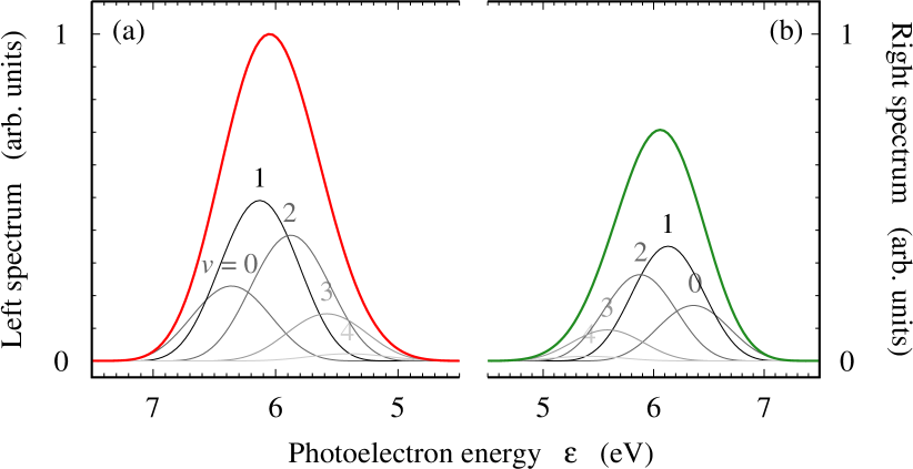
Figure 12: Photoelectron spectrum recorded on the left (a) and right (b) sides of molecule $\mathcal{B}$, upon single-photon ionization with a 40 fs light pulse of $37.23$ eV central frequency ($\mbox{HA}_{24}$ of a 800 nm field). Thin gray lines: $v$-resolved spectra ($v=0-4$, see peak labels); thick coloured lines: $v$-integrated spectra.

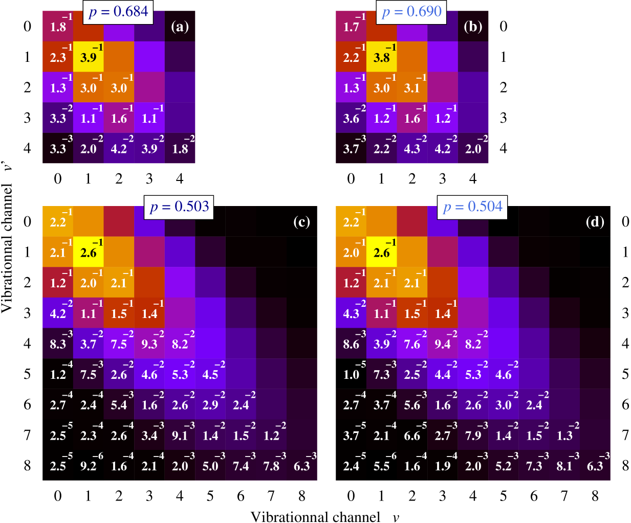
Figure 13: Photoionization of molecule $\mathcal{B}$ (top) and $\mathcal{C}$ (bottom) with a broadband XUV pulse (same simulations as Fig. 12). Modulus of the final ion’s reduced density matrix $\rho_{\text{\tiny ion}}(v,v^{\prime})$ [Eq. (LABEL:eqn:rhoion)] in the complete simulations (left) and in simulations at fixed conformations $R_{\text{\tiny vrt}}(v)$ (right). The values of the matrix elements’ modulii are provided in the lower triangles (the powers of ten are given in superscript). The matrices are displayed for the main open channels. Each one is normalized to have a trace equal to 1, consistently with the data displayed in Fig. 7. The value of the purity $p$ [Eq. (32)] is indicated at the top of each matrix.

As a last case, we now highlight the capacities of fixed-nuclei approaches to keep track of inter-channel coherences, when reconstructing the complete vibronic wave-packet out of a set of simulations performed at the $v$-dependent optimal conformations. To this end, we simulated the photoionization of molecules $\mathcal{B}$ and $\mathcal{C}$ with a broad XUV pulse of central frequency $\omega_{\text{\small xuv}}=37.23$ eV ($\mbox{HA}_{24}$ of a $800$ nm laser) and a duration of $8$ fs FWHM (3 fundamental IR cycles), in the 1-photon perturbative regime. The bandwidth of this pulse overlaps few vibrationnal channels in the photoelectron spectra, as shown in Fig. 12 for molecule $\mathcal{B}$. One therefore partially looses the vibrationnal resolution when looking at the $v$-integrated spectra, in contrast to the results obtained with narrower pulses, see for instance Fig. 10.

From the final channel-selective amplitudes in the continuum $a(v;\varepsilon,\theta_{\mbox{\tiny k}})$, we computed the reduced density matrix (RDM) of the ion in the final state as

$$\rho_{\text{\tiny ion}}(v,v^{\prime}) = \sum\limits_{\theta_{\mbox{\tiny k}}=0\degree,180\degree}\int\limits_{\Delta}\,d\varepsilon\,\left[a(v;\varepsilon,\theta_{\mbox{\tiny k}})\right]^{\star}a(v^{\prime};\varepsilon,\theta_{\mbox{\tiny k}})$$

where $[\ ]^{\star}$ denotes the complex conjugate and the spectral integration range $\Delta$ is restricted to the overall support of the photoelectron spectrum. The modulus of the RDM computed in the complete simulations for molecules $\mathcal{B}$ and $\mathcal{C}$ in the main vibrationnal channels are respectively shown in frames (a) and (c) of Fig. 13. For both molecules, we observe non vanishing off-diagonal elements which are signatures of coherences between overlapping channels ($|v^{\prime}-v|\lesssim 3$).

In the fixed nuclei simulations, we reconstructed the final RDM of the ion out of the amplitudes $\tilde{}a(R_{\text{\tiny opt}}(v);\varepsilon,\theta_{\mbox{\tiny k}})$ obtained in time-dependent simulations using the $v$-dependent vertical internuclear distances $R_{\text{\tiny vrt}}(v)$ for both molecules. The results are shown in frames (b) and (d) of Fig. 13 for molecules $\mathcal{B}$ and $\mathcal{C}$ respectively. The overall agreement with the complete simulations is excellent both for the populations (diagonal elements) and the coherences. To further evaluate the quality of these reconstructed vibrational RDM, we computed in each simulation the purity of the final state

$$p=\frac{\mbox{tr}(\rho_{\text{\tiny ion}}^{2})}{\mbox{tr}(\rho_{\text{\tiny ion}})^{2}},$$ (32)

where $\mbox{tr}()$ denotes the trace application. The purity values are indicated in Fig. 13 at the top of each matrix. The purity in fixed-nuclei results accurately match the ‘exact’ ones, within less than $1\%$, for both molecules. It is worth noting that, when using the $R_{\text{\tiny opt}}(v)$ conformations rather than the $R_{\text{\tiny vrt}}(v)$ ones, the fixed-nuclei simulations agree with the ‘exact’ ones with a $\sim 10\%$ accuracy only (results not shown). On the one hand, this underlines the sensitivity of the computed purity with respect to the conformations used in the fixed nuclei approach. On the other hand, it emphasizes the remarkable efficiency of the combined vertical conformations to reproduce the exact interchannel coherent dynamics.

V Summary and conclusion

We studied numerically how nuclear motion affects the dynamics of orientation-resolved photoemission in asymmetric diatomic model molecules presenting minimal vibronic couplings. We considered near-threshold photoemission in absence of any resonance, where the so-called stereo Wigner delays amount to few tens of attoseconds or less.

We have shown that the intrinsic molecular asymmetry results in an anisotropic electron-ion momentum sharing which, as slight as it may be, may prevent us from assigning unambiguously a stereo Wigner delay to the channel-averaged photoemission process. Indeed, a small asymmetry in the average photoelectron energy leads to stereo delay values that diverge when the (virtual) detection distance increases. This is circumvented by considering vibrationnally-resolved photoemission. However, on the theory side, comprehensive time-dependent vibronic simulations of molecules interacting with external fields are restricted to smaller molecules such as H₂ with a limited range of physical and numerical parameters, or to simplified low dimensional model molecules such as the ones used in the present work.

Therefore, we investigated ways of retrieving the vibrationnally-resolved photoemission dynamics revealed by the ‘complete’ vibronic simulations, out of more standard and broadly applicable time-independent approaches with fixed nuclei. We found empirically that each vibrationnal channel could be assigned an effective internuclear distance that reproduces the channel-resolved orientation-dependent photoemission yields and delays with a good accuracy. Furthermore, we identified a physical criterion, relying on the molecule’s ionization energies, that allows selecting a priori the $v$-dependent effective internuclear distances: It corresponds to the distance for which the vertical ionization potential matches the exact channel-dependent ionization potential. Identifying such unique effective molecular conformations is expected to work efficiently as long as the vertical ionization potential varies significantly when the molecular conformation is changed. Retrieving photoemission dynamics with vibrational resolution out of fixed nuclei simulation is also expected to work as long as photoemission takes place with little vibronic correlation, typically in smooth continua with sufficiently separated ionic vibrational levels.

Eventually, we assessed the relevence of the fixed-nuclei approach beyond the context in which we identified the effective internuclear distances. We first showed that it could be used to accurately simulate anisotropic vibrationnally-resolved RABBIT interferometry, both in terms of phase and amplitudes. Then, we investigated the fixed nuclei approach capacities to account for interchannel coherences in broadband photoionization of our model molecules, where the different channels significantly overlap. We showed that the fixed-nuclei approach could satisfactorily reproduce both the ion’s reduced density matrix and purity in the final state. This approach is thus of particular interest to model attosecond resolved photoemission dynamics in benchmark molecules without the need to resort to fully-fledged vibronic approaches. It could be applied to simulate attosecond time-resolved interferometry, highly non-linear processes such as strong field ionization [60] or molecular high-order harmonic generation [46, 61, 62, 63, 64], and to investigate ultrafast decoherence processes in molecule [35, 38, 44] of crucial importance in attochemistry.