Spectrum Coexistence of Satellite-borne Passive Radiometry and Terrestrial Next-G Networks

Abstract

Spectrum coexistence between terrestrial Next-G cellular networks and space-borne remote sensing (RS) is now gaining attention. One major question is how this would impact RS equipment. In this study, we develop a framework based on stochastic geometry to evaluate the statistical characteristics of radio frequency interference (RFI) originating from a large-scale terrestrial Next-G network operating in the same frequency band as an RS satellite. For illustration, we consider a network operating in the restricted L-band (1400-1427 MHz) with NASA’s Soil Moisture Active Passive (SMAP) satellite, which is one of the latest RS satellites active in this band. We use the Thomas Cluster Process (TCP) to model RFI from clusters of cellular base stations on SMAP’s antenna’s main- and side-lobes. We show that a large number of active clusters can operate in the restricted L-band without compromising SMAP’s mission if they avoid interfering with the main-lobe of its antenna. This is possible thanks to SMAP’s extremely low side-lobe antenna gains.

I Introduction

The spectrum crunch has fostered extensive research on the coexistence of different wireless technologies within the same spectrum. One case that has been gaining attention in recent years involves the use of passive Radio Frequency (RF) bands, which are solely devoted to passive sensing applications such as remote sensing and radio astronomy, for active wireless communications. Specifically, the coexistence of terrestrial active wireless communications and Earth Exploration Satellite Services (EESS) is becoming a central topic of discussion [1]. A major question that needs to be answered is how and to what extent Radio Frequency Interference (RFI) would impact such EESS satellites.

While current research primarily examines spectrum sharing between terrestrial cellular networks and terrestrial passive sensing technologies, such as the Radio Dynamic Zones (RDZ) proposed by [2] and the Shared Spectrum Access Zones (SSAZ) for the coexistence of cellular wireless communications and terrestrial radio astronomy systems proposed by [3], in this study, we develop a mathematical framework to model the RFI originating from a large-scale terrestrial cellular network and its impact on an EESS satellite. Specifically, we imagine clusters of cellular base stations exposed to an EESS satellite, where each cluster has a number of base stations active in the same frequency band as the satellite. To account for the randomness of the position of the clusters on Earth and the number of active cells within a cluster, we use the Thomas Cluster Process (TCP) from stochastic geometry [4].

For illustration, we develop our model based on the National Aeronautics and Space Administration (NASA) Soil Moisture Active Satellite (SMAP) [5], which is one of the latest RS satellites active in the restricted L-band ($1400-1427$ MHz). We develop the characteristic function of RFI at both the main- and side-lobes of SMAP’s antenna. Using the characteristic function, we then derive the statistical properties of the RFI, namely, its average, variance, and higher central moments We also demonstrate that, due to the very low side-lobe gains of SMAP’s antenna, a large number of terrestrial clusters can be active while exposed to SMAP’s side-lobe without compromising the accuracy of SMAP’s measurements.

The paper is organized as follows. In Section II we introduce SMAP’s measurement mechanism, our methodology for RFI analysis, and other preliminaries. Section III is the main RFI analysis section. Section IV is the simulations and results section. Section V is the conclusion section.

II Preliminaries

II-A SMAP & Brightness Temperature

As depicted in Figure 1, SMAP has a 6-meter-wide conically-scanning golden mesh reflector with a 3-dB antenna beam-width of $2.4{\degree}$ that projects a footprint of roughly $40\times 40$ km² with an incident angle of $40^{\degree}$ at an altitude of $685$ $km$. An Ortho-Mode Transducer (OMT) feedhorn collects the reflected radiations from the mesh reflector and duplexes them separately into vertical and horizontal polarizations. Figure 2 shows a 2-dimensional cut of SMAP’s antenna gain for the vertical polarization. Through sectorization, which is a common method in stochastic geometry, we represent SMAP’s antenna gain for each polarization $(p)$ as:

$$g=\left\{\begin{array}[]{ll}g_{(ml)},&\mbox{if }|d|\leq 1.2{\degree},\\ g_{(sl)},&\mbox{if }|d|>1.2{\degree},\end{array}\right.$$ (1)

where $(ml)$ and $(sl)$ stand for main-lobe and side-lobe, respectively, and $|d|$ is the deviation from the main-lobe axis. For each polarization $(p)$, SMAP separately captures the brightness temperature of soil, $t_{soil}^{(p)}$ (in Kelvin), from the antenna footprint by capturing the soil’s natural passive thermal radiations. These brightness temperature measurements can be translated to soil moisture content using models like the Tau-Omega mode [5]. We use the Nyquist noise formula [6] to convert electromagnetic power to brightness temperature as:

$$t^{(p)}=\frac{\mathrm{p}^{(p)}}{k_{b}\beta},$$ (2)

where $\mathrm{p}^{(p)}$ is the electromagnetic power received by polarization $(p)$, $k_{b}$ is the Boltzmann constant, and $\beta$ is the radio frequency bandwidth.

Note 1.

Due to the symmetrical nature of SMAP’s antenna gain for both polarizations, as well as the symmetry in the RFI scenario, we assume identical RFI characteristics for both of SMAP’s polarizations. Thus, the discussions that follow hold true for SMAP’s measurements in both polarizations.

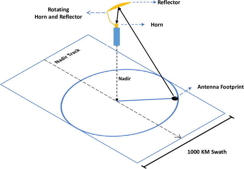
Figure 1: Horn and reflector rotation, beam footprint of the reflector, and SMAP’s nadir track.

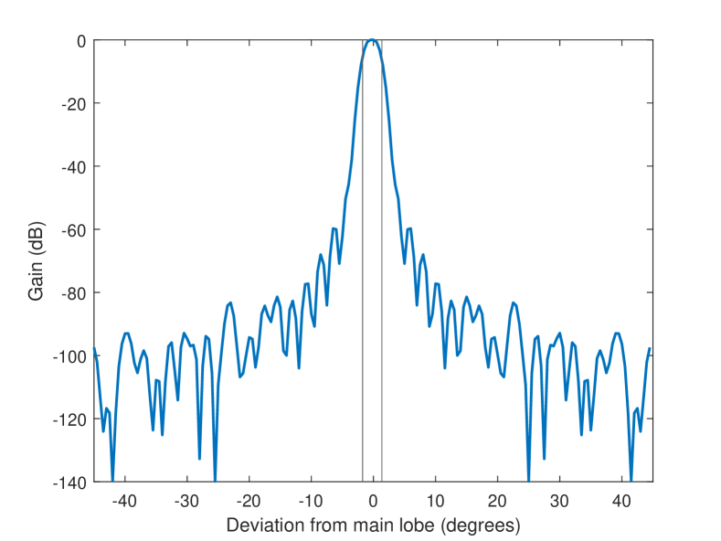
Figure 2: A 2-dimensional cut of SMAP’s conical antenna gain for the vertical polarization. The gain for the horizontal polarization is similar. The two vertical lines show the $2.4^{\degree}$ antenna beam-width.

II-B Methodology for RFI Analysis

In this section, we provide a concise explanation of the underlying logic guiding our analysis of RFI on SMAP. SMAP’s measurements for each polarization can be seen as:

$$t_{meas}=t_{soil}+T_{RFI},$$ (3)

where $T_{RFI}$ denotes the RFI temperature at SMAP. Since $T_{RFI}$ is a random variable, it causes uncertainty in SMAP’s measurements. According to SMAP’s documentation, uncertainties below threshold value $\tau=1.3K$ are acceptable for SMAP’s measurements [5]. To model $T_{RFI}$ from a large terrestrial network, we imagine a set of $\{i\}$ Base Station (BS) clusters on the Earth-cut exposed to SMAP, where each cluster $i$ comprises a set of $\{j\}_{i}$ BSs, each BS_ij has a (maximum) total electromagnetic transmission power $p_{tx}$, and $P_{ij}$ is the amount of power received by SMAP from BS_ij. Clusters $\{i\}_{(ml)}\subset\{i\}$ are located on SMAP’s main-lobe antenna footprint and clusters $\{i\}_{(sl)}\subset\{i\}$ are exposed to SMAP’s side-lobe. Accordingly, $T_{RFI}$ in (3), can be decomposed into its main- and side-lobe components as:

$$T_{RFI}=T_{(ml)}+T_{(sl)},$$ (4)

where

$$T_{(l)}=\sum\nolimits_{\{i\}_{(l)}}\sum\nolimits_{\{j\}_{i}}T_{ij}$$ (5)

with $$T_{ij}=\frac{P_{ij}}{k_{b}\beta}$$ (6)

where $(l)$ is either $(ml)$ or $(sl)$. Assessing each $P_{ij}$ would be a complicated function of BS_ij antenna angles, obstructions in the environment, and SMAP’s elevation angle relative to BS_ij. However, based on Free Space Path Loss (FSPL), we note that:

$$P_{ij}\in\left[0,\;g\left(\frac{c}{4\pi fd_{ij}}\right)^{\alpha}p_{tx}\right]$$ (7)

and therefore, according to (6),

$$T_{ij}\in\left[0,\;g\eta\omega^{\alpha}d_{ij}^{-\alpha}\right],$$ (8)

where $\eta=\frac{p_{tx}}{k_{b}\beta}$, $\omega=\left(\frac{c}{4\pi f}\right)$, $g$ is the gain of SMAP’s antenna (based on (1), $g=g_{(ml)}$ if $i\in\{i\}_{(ml)}$, and $g=g_{(sl)}$ if $i\in\{i\}_{(sl)}$), $c$ is the speed of light, $f$ is the frequency, $d_{ij}$ is the distance of BS_ij to SMAP, and $\alpha>2$ is the path loss exponent. In (7), we ignore atmospheric loss since it is proven to have a negligible effect in the L-band [5]; however, this means that our model slightly overestimates the RFI.

We acknowledge that transient phenomena like fading and shadowing can cause temporary spikes in electromagnetic power. SMAP’s documentation indicates a full-band integration time of $300\leavevmode\nobreak\ \micro s$ and a sub-band integration time of approximately $1.2\leavevmode\nobreak\ ms$, emphasizing the need to address fast-fading effects. While fast-fading models could establish an upper limit for $P_{ij}$ with confidence, we have opted to omit this in our current study for future research. Instead, for assessing maximum RFI on SMAP, we use $T_{ij}:=g\eta\omega^{\alpha}d_{ij}^{-\alpha}$ in (5). This is akin to assuming the worst-case scenario, where all the transmission power from a single base station is directed solely towards the satellite.

II-C Geometric Assumptions

As depicted in Figure 3, the Earth’s center is the origin $(0,0,0)$ and SMAP is located at the point $\mathtt{h}=(0,0,h)$, where $h$ is the distance of SMAP from the Earth’s center.

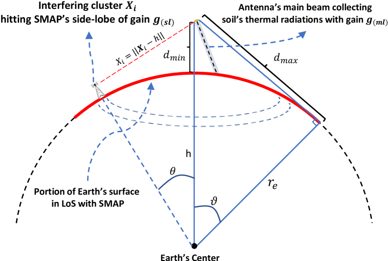
Figure 3: 2-dimensional representation of the Earth-cut exposed to the satellite. The red curve represents the maximum extent of the Earth-cut exposed.

The area exposed to the satellite, shown with the red cap and encircled in $\theta\in[0,\vartheta]$ in Figure 3, is defined with the Borel-set $\mathcal{B}=\left\{\lVert\mathtt{x}\lVert=r_{e},\;\frac{\mathtt{x}\cdot\mathtt{h}}{\lVert\mathtt{x}\lVert\lVert\mathtt{h}\lVert}\geq\cos{(\vartheta)}\right\}$ in $\mathbb{R}^{3}$ measure space, where $r_{e}$ is the Earth radius, $\lVert\cdot\lVert$ is the Euclidean norm, and $\cos{(\vartheta)}=\frac{r_{e}}{h}$. We define $\mathcal{B}_{(ml)}\subset\mathcal{B}$ as SMAP’s antenna footprint projected on Earth and $\mathcal{B}_{(sl)}=\mathcal{B}\big{\backslash}\mathcal{B}_{(ml)}$ as the set of area exposed to the side-lobe of SMAP’s antenna.

Let $\Psi=\{\mathbb{X}_{i},i\in\mathbb{N}\}\subset\mathcal{B}$ denote a parent Poisson Point Process (PPP) with intensity measure $\Lambda(d\mathtt{x})$, where $\mathbb{X}_{i}$ denotes a cluster center. For simplicity we use a homogeneous PPP such that $\Lambda(d\mathtt{x})=\lambda_{c}$. According to Figure 3, the minimum distance of a cluster center to SMAP is $d_{min}=h-r$, while the maximum distance is $d_{max}=\sqrt{h^{2}-r_{e}^{2}}$. With $\psi=\{\mathtt{x}_{i}\}$ defined as a realization of $\Psi$, for each point $\mathtt{x}\in\psi$, we associate an independent and identically distributed (i.i.d) offspring PPP $\Xi_{\mathtt{x}}$. Each cluster $\Xi_{\mathtt{x}}$ consists of $N$ i.i.d random points (BSs) where, according to a Thomas Cluster Process (TCP), $N\sim\textsf{Pois}{(\lambda_{BS})}$. We define $\Phi\sim\mathcal{P}(\lambda_{c},\lambda_{BS})$, where

$$\Phi=\bigcup\nolimits_{\mathbb{x}\in\Psi}\left(\mathbb{x}+\Xi_{\mathbb{x}}\right).$$ (9)

Accordingly, the cluster centers located in SMAP’s main- and side-lobes are respectively $\Psi_{(ml)}=\Psi(\mathcal{B}_{(ml)})$ and $\Psi_{(sl)}=\Psi\big{\backslash}\Psi_{(ml)}$, and their respective clusters are $\Phi_{(ml)}$ and $\Phi_{(sl)}$.

Note 2.

Defining $X_{i}=\lVert\mathbb{X}_{i}-\mathtt{h}\lVert$ as the distance of terrestrial cluster center $\mathbb{X_{i}}$ to SMAP and $x_{i}$ as its realization, we assume that the cluster’s dispersion $\ll x_{i}$, since an urban area is on the order of a few kilometers, while the cluster distance to SMAP is more than $d_{min}=685$ km. Thus, for simplicity, we assume that the off-spring (BSs) within each cluster are equidistant (with distance $x_{i}$) to SMAP.

III RFI Analysis

To assess the RFI brightness temperature $T_{RFI}$ on SMAP as defined in (4), we analyze the statistical properties of RFI on SMAP’s main- and side-lobes, i.e., its average, variance, and higher central moments (skewness and kurtosis). For this purpose, we use the concepts of Cumulants and Cumulant Generating Functions (CGFs).

Definition 1.

The CGF of random variable $X$ is defined as:

$$K(t)=\log\mathds{E}[e^{tX}],$$ (10)

which is the $\log$ of the Moment Generating Function (MGF) $M(t)=\mathds{E}[e^{tX}]$ of random variable $X$. Accordingly the $n$th cumulant of $X$ is as follows:

$$k_{n}=K^{n}(0),$$ (11)

where $K^{n}(t)$ denotes the $n$th derivative of $K(t)$.

Remark 1.

For random variable $X$, $k_{1}=\mu_{0}$, where $\mu_{0}$ is the first moment of $X$, i.e., $\mathds{E}[X]$. For $n\in\{2,3\}$, $k_{n}=\mu_{n}$, where $\mu_{n}$ is the $n$th central moment of $X$. Consequently, the variance of $X$ is its $2$nd central moment, i.e., $k_{2}=\mu_{2}$. Lastly, higher order central moments $\mu_{n}$ for $n>3$ can be acquired by a combination of cumulants of $X$. For example, $\mu_{4}=k_{4}+3(k_{2})^{2}$.

Based on Definition 1 and Remark 1, we shift our focus on finding the MGF of $T_{(ml)}$ and $T_{(sl)}$ defined in (4). For this purpose, we start with the MGF of RFI brightness temperature of one cluster of BSs.

III-A MGF for one Cluster

One key quantity that can help us determine the total RFI brightness temperature at SMAP is the maximum RFI brightness temperature contributed by one cluster. Assuming the cluster is located at point $\mathtt{x}\in\psi$ and comprises $N$ BSs that are equidistant to SMAP, we have:

$$T_{cluster}(\mathtt{x})=g\eta\omega^{\alpha}\lVert\mathtt{x}-\mathtt{{\color[rgb]{0,0,0}{h}}}\lVert^{-\alpha}N.$$ (12)

Lemma 1.

For a cluster located at point $\mathtt{x}\in\psi$ with $N\sim\textsf{Pois}(\lambda_{BS})$ equidistant BSs (with distance $x=\lVert\mathtt{x}-\mathtt{h}\lVert$) to the satellite, the MGF of (12) is as follows:

$$M_{cluster}(t;\;x,\;g)=\\ \exp\left(\lambda_{BS}\left(-1+\exp\left(g\eta\omega^{\alpha}x^{-\alpha}t\right)\right)\right).$$ (13)

Proof.

Since $N$ is a Poisson random variable, the MGF of $N$ is $M_{N}(t)=\exp\left(\lambda_{BS}(e^{t}-1)\right)$. By setting $t:=g\eta\omega^{\alpha}x^{-\alpha}t$, we acquire (13). ∎

$T_{\text{cluster}}(\mathtt{x})$ in (12) is the fundamental unit of RFI brightness temperature in our model. We obtain its series expansion to facilitate the calculation of RFI brightness temperature cumulants later on.

Lemma 2.

The series expansion of (13) is as follows:

$$M_{cluster}(t;\;x,\;g)=\sum_{n=0}^{\infty}p_{n}(\lambda_{BS})\left(g\eta\omega^{\alpha}x^{-\alpha}\right)^{n}\frac{t^{n}}{n!},\vspace{-2mm}$$ (14)

with:

$$p_{n}(\lambda_{BS})=\sum\nolimits_{i=0}^{n}S(n,i)\lambda_{BS}^{i},$$ (15)

where $S(n,i)$ is the Stirling number of the second kind.

Proof.

From [7], we know that:

$$\exp\left(v(e^{t}-1)\right)=\sum_{n=0}^{\infty}B_{n}(v)\frac{t^{n}}{n!},$$ (16)

where $B_{n}(v)$ is the Bell polynomial of order $n$, and can be expanded as:

$$B_{n}(v)=\sum\nolimits_{i=0}^{n}S(n,i)v^{i}.$$ (17)

By setting $t:=g\eta\omega^{\alpha}x^{-\alpha}t$ and $v=\lambda_{BS}$ in (16), we acquire (14). ∎

III-B MGF on SMAP’s Main- and Side-lobes

III-B1 SMAP’s main-lobe

The RFI brightness temperature $T_{(ml)}$ on SMAP’s main-lobe is caused by all the clusters $\mathtt{x}\in\psi_{(ml)}$ in SMAP’s main-lobe antenna footprint: i.e.,

$$T_{(ml)}=\sum\nolimits_{\mathbb{X}_{i}\in\psi_{(ml)}}T_{cluster}(\mathbb{X}_{i}).$$ (18)

Note 3.

Given that SMAP’s antenna footprint is relatively small compared to the distance to the satellite, we assume a uniform distribution, envisioning that all cluster centers within the main-lobe antenna footprint ($\mathtt{x}\in\psi^{(ml)}$) are approximately equidistant from the satellite. Under this assumption, the distance to the satellite for the clusters in the main-lobe is:

$$d_{(ml)}=h\cos{(40{\degree})}-\sqrt{r_{e}^{2}-h^{2}\sin^{2}{(40{\degree})}}.$$ (19)

Lemma 3.

With the assumption of $M\sim\textsf{Pois}(\Lambda)$ equidistant $d_{(ml)}$ clusters from the satellite located in SMAP’s main-lobe antenna footprint $\mathcal{B}_{(ml)}$, where $\Lambda=\lambda_{c}\text{v}^{2}(\mathcal{B}_{(ml)})$ and $\text{v}^{2}(\cdot)$ is a Lebesgue measure in $\mathbb{R}^{2}$, the MGF of $T_{(ml)}$ defined in (18) is as follows:

$$M_{(ml)}(t)=\\ \exp\left(40^{2}\lambda_{c}\left(-1+M_{cluster}(t;\;d_{(ml)},\;g_{(ml)})\right)\right),$$ (20)

where $M_{cluster}(t;\;x,\;g)$ is defined in (13).

Proof.

Refer to Appendix A. ∎

III-B2 SMAP’s side-lobe

In this section, we investigate the maximum RFI brightness temperature $T_{(sl)}$ on SMAP’s side-lobe defined in (4), which we can rewrite as:

$$T_{(sl)}=\sum\nolimits_{\mathbb{X}_{i}\in\Psi_{(sl)}}T_{cluster}(\mathbb{X}_{i}),$$ (21)

where $T_{cluster}(\mathbb{X}_{i})$ is defined in (12).

Lemma 4.

The MGF of (21) is as:

$$M_{(sl)}(t)=$$

$$\exp{\left(-2\pi\left(\frac{r_{e}}{h}\right)\lambda_{c}\int_{d_{min}}^{d_{max}}\left(1-M_{cluster}(t;\;x,\;g_{(sl)})\right)x\,dx\right)}$$ (22)

where $M_{cluster}(t;\;x,\;g)$ is defined in (13), and $d_{min}=h-r_{e}$ and $d_{max}=\sqrt{h^{2}-r^{2}_{e}}$.

Proof.

Refer to Appendix B. ∎

III-C Cumulants of RFI Brightness Temperature on SMAP’s Main- and Side- Lobes

Now that we have the MGFs of $T_{(ml)}$ and $T_{(sl)}$, we are able to acquire their cumulants.

Lemma 5.

The $n$th cumulant of RFI brightness temperature $T_{(ml)}$ on SMAP’s main-lobe, defined in (18), is as follows:

$$k_{n}^{(ml)}=40^{2}g_{(ml)}^{n}\eta^{n}\omega^{n\alpha}\lambda_{c}p_{n}(\lambda_{BS})d_{(ml)}^{-n\alpha},$$ (23)

where $p_{n}(\lambda_{BS})$ is defined in (15).

Proof.

The cumulants of $T_{(ml)}$ can be acquired using its MGF as defined in (20) and definition 1. ∎

Corollary 1.

The expected value of $T_{(ml)}$ defined in (18) is:

$$\mathds{E}[T_{(ml)}]=40^{2}g_{(ml)}\eta\omega^{\alpha}\lambda_{c}\lambda_{BS}d_{(ml)}^{-\alpha}.$$ (24)

Proof.

Based on remark 1, the expected value of $T_{ml}$ is its first cumulant defined in (23). ∎

Corollary 2.

The variance of $T_{(ml)}$ defined in (18) is as:

$$Var[T_{(ml)}]=40^{2}g_{(ml)}^{2}\eta^{2}\omega^{2\alpha}\lambda_{c}(\lambda_{BS}^{2}+\lambda_{BS})d_{(ml)}^{-2\alpha}.$$ (25)

Proof.

Based on remark 1, the variance of $T_{(ml)}$ is its second cumulant defined in (23). ∎

Lemma 6.

The $n$th cumulants of the RFI brightness temperature $T_{(sl)}$ on SMAP’s side-lobe, defined in (21), is as follows:

$$k_{n}^{(sl)}=\\ \frac{2\pi}{2-n\alpha}\left(\frac{r_{e}}{h}\right)g_{(sl)}^{n}\eta^{n}\omega^{n\alpha}\lambda_{c}p_{n}(\lambda_{BS})\left(d_{max}^{2-n\alpha}-d_{min}^{2-n\alpha}\right),$$ (26)

where $p_{n}(\lambda_{BS}$) is defined in (15).

Proof.

The cumulants of $T_{(sl)}$ can be acquired using its MGF as defined in (22) and definition 1. ∎

Corollary 3.

The expected value of $T_{(sl)}$ defined in (21) is:

$$\mathds{E}[T_{(sl)}]=\\ \frac{2\pi}{2-\alpha}\left(\frac{r_{e}}{h}\right)g_{(sl)}\eta\omega^{\alpha}\lambda_{c}\lambda_{BS}\left(d_{max}^{2-\alpha}-d_{min}^{2-\alpha}\right).$$ (27)

Proof.

Based on remark 1, the expected value of $T_{(sl)}$ is its first cumulant defined in (26). ∎

Corollary 4.

The variance of $T_{(ml)}$ defined in (18) is:

$$Var[T_{(sl)}]=\\ \frac{2\pi}{2-2\alpha}\left(\frac{r_{e}}{h}\right)g_{(sl)}^{2}\eta^{2}\omega^{2\alpha}\lambda_{c}(\lambda_{BS}^{2}+\lambda_{BS})\left(d_{max}^{2-2\alpha}-d_{min}^{2-2\alpha}\right).$$ (28)

Proof.

Based on remark 1, the variance of $T_{(sl)}$ is its second cumulant defined in (26). ∎

IV Numerical Results

In this section, we evaluate the RFI brightness temperature statistics at both SMAP’s main- and side-lobes based on the analysis in the previous sections. The simulation parameters are given in Table I. Based on this table, an average of one cluster exists in every $10000$ $km^{2}$ and, on average, $2500$ BS clusters exist in the area exposed to the satellite. We also set SMAP’s side-lobe gain to a conservative $-55$ dB.

Table I: LIST OF CONFIGURATION PARAMETERS FOR PERFORMANCE EVALUATION

Element	Value
Intensity of clusters ($\lambda_{C}$)	$1$ cluster (large city) every $10000$ $km^{2}$
Intensity of active BS ($\lambda_{BS}$)	$50$, $100$, $200$ BSs per cluster
Path loss exponent ($\alpha$)	(2 , 2.2]
BS transmission power ($p_{tx}$)	$3.5$ Watts per BS
Boltzmann’s constant ($k_{b}$)	$1.380649\times 10^{-23}$ m2kg s-2K-1
Light speed ($c$)	$300,000$ $km$ $s^{-1}$
SMAP’s main-lobe antenna gain ($g_{(ml)}$)	$0$ dB
SMAP’s side-lobe antenna gain ($g_{(sl)}$)	$-55$ dB
Central Carrier frequency of BS ($f$)	$1.413$ GHz
BS transmission bandwidth ($\beta$)	$24$ MHz
Earth radius ($r_{e}$)	$6371$ km
SMAP’s distance to Earth’s center ($h$)	$7056$ km
Min. possible distance to SMAP ($d_{\min}$)	$h-r=685$ km
Max. possible distance to SMAP ($d_{\max}$)	$\sqrt{h^{2}-r^{2}}=3032.7$ km

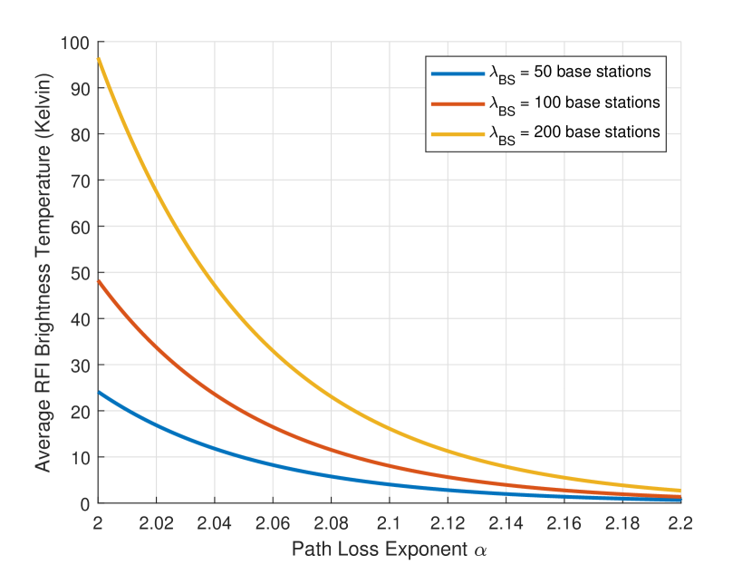
(a) Main-lobe average RFI brightness temperature.

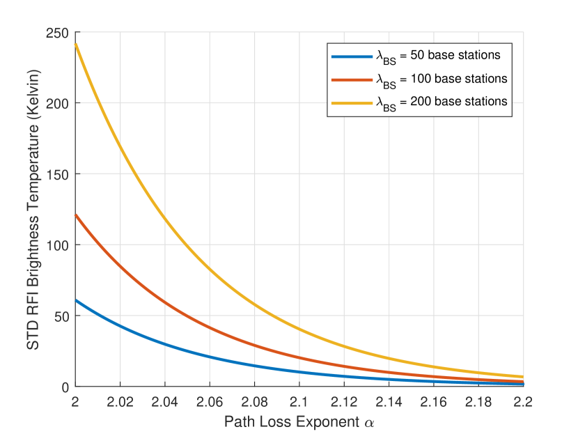
(b) Main-lobe STD of RFI brightness temperature.

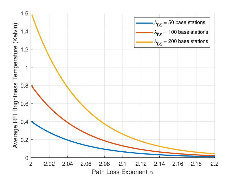
(c) Side-lobe average RFI brightness temperature

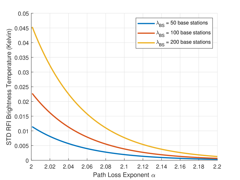
(d) Side-lobe STD of RFI brightness temperature.

Figure 4: Average and Standard Deviation of RFI brightness temperature on SMAP’s main- and side-lobes for average $\lambda_{BS}=50,\;100,\;200$ active BSs in a cluster. On average $125,\;250$ and $500$ thousand base stations are exposed to SMAP’s side-lobe, while only, on average, $7,\;14$ and $28$ base stations are exposed to SMAP’s main-lobe.

Due to space limitations, we only assess the average and standard deviation (STD) of RFI brightness temperature at SMAP’s main- and side-lobes. We use these metrics to determine if the values fall within an acceptable error range. Figure 4 illustrates the findings. In Figure 4(a), the average RFI brightness temperature at SMAP’s main-lobe exceeds the acceptable threshold $\tau=1.3K$, ranging from $20$ to $100$ Kelvin. Figure 4(b) shows a high standard deviation in the range of hundreds, indicating extreme uncertainty in RFI. Notably, $7$ to $28$ base stations, on average, contribute to these RFI characteristics.

Now we focus on RFI brightness temperature on SMAP’s side-lobe depicted in Figures 4(c) and 4(d). As observable in figure 4(c), for clusters with an average of $50$ and $100$ active BSs, the average RFI brightness temperature falls within the acceptable threshold of $1.3K$, while for clusters of average $200$ active BSs, the average RFI brightness temperature slightly exceeds the limit. Also, from Figure 4(d), we see extremely low STD values for RFI brightness on SMAP’s side-lobe, which is an indicator of extremely low uncertainty in RFI.

V Conclusion

In this paper, we introduced an innovative method using cluster processes in stochastic geometry to evaluate RFI brightness temperature on passive remote sensing satellites. Our model is tailored to NASA’s SMAP satellite, passively operating in the restricted L-band $1400$ to $1427$ MHz. Interestingly, our findings show that , while avoiding active base stations in main-lobe antenna footprint through satellite positioning, SMAP’s antenna’s remarkably low side-lobe gains allow for numerous active co-channel cellular base stations without compromising measurement precision.

Appendix A Proof to Lemma 3

Since SMAP’s main-lobe antenna footprint is roughly $40^{2}$ $km^{2}$, we note that $\Lambda=40^{2}\lambda_{c}$. Thus, conditioned on $M$ we note that:

$$M_{(ml)}(t)=\mathds{E}_{M}\left[\mathds{E}\left[\exp\left(t\sum\nolimits_{M}T_{cluster}(\mathtt{x})\right)\right]\right].$$ (29)

The inner $\mathds{E}[\cdot]$ is the MGF of the sum of $M$ clusters defined in (12), and based on (13), can be expressed as:

$$\mathds{E}\left[\exp\left(t\sum\nolimits_{m}T_{cluster}(\mathtt{x})\right)\right]=\\ \left(M_{cluster}(t;\;d_{(ml)},\;g_{(ml)})\right)^{m}.$$ (30)

Accordingly, (29) can be expanded as:

$$M_{(ml)}(t)=\sum_{m=0}^{\infty}\frac{e^{-\Lambda}\Lambda^{m}}{m!}\left(M_{cluster}(t;\;d_{(ml)},\;g_{(ml)})\right)^{m},$$ (31)

which is equivalent to (20).

Appendix B Proof to Lemma 4

For ease of notation, in (21) we define $T_{\mathbb{X}_{i}}:=T_{cluster}(\mathbb{X}_{i})$. Accordingly, the MGF of (21) is as:

$$M_{(sl)}(t) =\mathds{E}\left[e^{tT_{(sl)}}\right]$$

$$=\mathds{E}_{\Psi,\{T_{\mathbb{X}_{i}}\}}\left[\prod\nolimits_{\mathbb{X}_{i}\in\Psi^{(sl)}}e^{tT_{\mathbb{X}_{i}}}\right].$$ (32)

Due to the initial assumption of the independence of clusters, we move the expectation with respect to $\{T_{\mathbb{X}_{i}}\}$ inside the product as:

$$\mathds{E}_{\Psi_{(sl)}}\left[\prod\nolimits_{\mathbb{X}_{i}\in\Psi_{(sl)}}\mathds{E}\left[e^{tT_{\mathbb{X}_{i}}}\right]\right],$$ (33)

which is the Probability Generating Functional (PGFL) [8] of $g(\mathtt{x})=\mathds{E}\left[e^{tT_{\mathtt{x}}}\right]$ over the set $\mathcal{B}_{(sl)}$ and can be written as:

$$\small\mathcal{P}_{\Psi_{(sl)}}(g)=\mathds{E}_{\Psi_{(sl)}}\left[\prod_{\mathrm{X}_{i}\in\Psi_{(sl)}}g(\mathrm{X}_{i})\right]\\ =\exp\left(-\int_{\mathcal{B}_{(sl)}}\left(1-g(\mathtt{x})\right)\,\Lambda(d\mathtt{x})\right),$$ (34)

where, based on Fig. (3), in spherical coordinates for equidistant points to SMAP for a PPP with intensity $\lambda_{c}$:

$$\Lambda\left(d\mathtt{x}\right)=2\pi r^{2}\lambda_{c}\sin(\theta)\;d\theta.$$ (35)

We note that $g(\mathtt{x})$ is the MGF of RFI brightness temperature of a cluster at point $\mathtt{x}\in\mathcal{B}_{(sl)}$ as in (13), which we note here with $g(\mathtt{x})=M_{cluster}(t;\;\lVert\mathtt{x}-\mathtt{h}\lVert,\;g_{(sl)})$, where $x=\lVert\mathtt{x}-\mathtt{h}\lVert$ is the distance to SMAP. From Fig. (3), and using the law of cosines, we note that:

$$x=\left(r_{e}^{2}+h^{2}-2hr_{e}\cos(\theta)\right)^{\frac{1}{2}},$$ (36)

with:

$$dx=hr_{e}\sin(\theta)\left(r_{e}^{2}+h^{2}-2hr_{e}\cos(\theta)\right)^{-\frac{1}{2}}\;d\theta$$

$$\Rightarrow x\; dx=hr_{e}\sin(\theta)\;d\mathtt{\theta}.$$ (37)

Comparing (35) and (37), we note that:

$$\Lambda\left(d\mathtt{x}\right)=2\pi\left(\frac{r_{e}}{h}\right)\lambda_{c}x\;dx,$$ (38)

where $x$ is in the range of $d_{max}$ and $d_{min}$. By substituting (38) in (34), we will have (22).

References

- [1] M. Polese, X. Cantos-Roman, A. Singh, M. J. Marcus, T. J. Maccarone, T. Melodia, and J. M. Jornet, “Coexistence and spectrum sharing above 100 ghz,” arXiv preprint arXiv:2110.15187, 2021.
- [2] M. Zheleva, C. R. Anderson, M. Aksoy, J. T. Johnson, H. Affinnih, and C. G. DePree, “Radio dynamic zones: Motivations, challenges, and opportunities to catalyze spectrum coexistence,” IEEE Communications Magazine, 2023.
- [3] Y. R. Ramadan, H. Minn, and Y. Dai, “A new paradigm for spectrum sharing between cellular wireless communications and radio astronomy systems,” IEEE Transactions on communications, vol. 65, no. 9, pp. 3985–3999, 2017.
- [4] M. Afshang, H. S. Dhillon, and P. H. J. Chong, “Modeling and performance analysis of clustered device-to-device networks,” IEEE Transactions on Wireless Communications, vol. 15, no. 7, pp. 4957–4972, 2016.
- [5] D. Entekhabi, S. Yueh, P. E. O’Neill, K. H. Kellogg, A. Allen, R. Bindlish, M. Brown, S. Chan, A. Colliander, W. T. Crow et al., “Smap handbook–soil moisture active passive: Mapping soil moisture and freeze/thaw from space,” 2014.
- [6] C. S. Turner, “Johnson-nyquist noise,” url: http://www. claysturner. com/dsp/Johnson-NyquistNoise, 2012.
- [7] K.-W. Hwang, C. S. Ryoo, and N. S. Jung, “Differential equations arising from the generating function of the (r, )-bell polynomials and distribution of zeros of equations,” Mathematics, vol. 7, no. 8, p. 736, 2019.
- [8] F. Baccelli and B. Błaszczyszyn, “Stochastic geometry and wireless networks: Volume i theory,” Foundations and Trends® in Networking, vol. 3, no. 3–4, pp. 249–449, 2010. [Online]. Available: http://dx.doi.org/10.1561/1300000006