Relaxation of weakly collisional plasma: continuous spectra, Landau eigenmodes, and transition from the collisionless to the fluid limit

Abstract

The relaxation of a weakly collisional plasma, which is of fundamental interest to laboratory and fusion plasmas as well as astrophysical plasmas, is described by the self-consistent Boltzmann-Poisson equations with the Lenard-Bernstein collision operator. We perform a perturbative analysis of the Boltzmann-Poisson equations, and obtain, for the first time, exact analytic solutions which enable definitive resolutions to some long-standing controversies regarding the impact of weak collisions on the continuous spectra and Landau eigenmodes. Unlike some previous studies, we retain both damping and diffusion terms in the collision operator. We find that the linear response is a temporal convolution of two types of contribution: a continuum that depends on the continuous velocities of particles, and another, consisting of discrete normal modes that are coherent modes of oscillation of the entire system. The normal modes are exponentially damped over time due to collective effects or wave-particle interactions (Landau damping), as well as collisional dissipation. The continuum is also damped by collisions, but somewhat differently than the normal modes. Up to a collision time, which is the inverse of the collision frequency $\nu_{\rm c}$, the continuum decay is driven by the diffusion of particle velocities and is super-exponential, occurring over a timescale $\sim\nu^{-1/3}_{\rm c}$. After a collision time, however, the continuum decay is driven by the collisional damping of particle velocities and diffusion of their positions, and occurs exponentially over a timescale $\sim\nu_{\rm c}$. This hitherto unknown, slow exponential decay causes perturbations to damp the most on scales comparable to the mean free path, but very slowly on larger scales. This leads to the establishment of local thermal equilibrium (LTE), which is the essence of the fluid limit. The long-term decay of the plasma response is driven by the normal modes on scales smaller than the mean free path, but, on larger scales, is governed by a combination of the slowly decaying continuum and the least damped normal mode. Our analysis of the relaxation of weakly collisional plasmas firmly establishes a long-sought connection between the collisionless and fluid limits.

I Introduction

The relaxation of plasma is a complicated many-body problem with rich phenomenology. Many astrophysical and space plasmas are nearly collisionless and are often described by the collisionless Boltzmann (also known as the Vlasov) equation, widely discussed in textbooks. However, no matter how infrequent the collisions, no plasma in nature or a terrestrial laboratory is strictly collisionless, so in practical terms one may also treat a collisionless plasma as the zero-collision limit of a weakly collisional plasma. Furthermore, if the collision operator is of the Fokker-Planck type, the collision frequency typically multiplies the highest velocity derivative in the kinetic equation. Taking the limit of zero collisions is then a subtle problem, requiring the use of singular perturbation theory. It should then not be surprising if the results obtained in the zero-collision limit of the weakly collisional problem differ qualitatively from those obtained by solving the collisionless problem. The physical effect of weak collisions tends to regulate extreme filamentation in phase space, much in the same way as viscosity tends to regulate near-singular vortex structures in fluids governed by the Navier-Stokes equation.

These considerations have deep implications for the thermodynamics of many-body systems. It is well known that the Vlasov equation does not possess an H-theorem, but the Boltzmann equation does. The Vlasov equation has a denumerably infinite number of Casimirs (invariants). How many of them (if any) survive in the weakly collisional limit? And how do they influence the turbulent relaxation of a weakly collisional plasma? The Vlasov equation, despite the occurrence of Landau damping, is time-reversible, as demonstrated by the phenomenon of plasma echoes. How do weak collisions affect the time-evolution of echoes? Answering some of these questions requires a detailed investigation of the nonlinear relaxation of weakly collisional plasmas. However, before solving the nonlinear problem, we must properly understand the perturbative regime of relaxation. This paper addresses some of the open issues in the perturbative relaxation of weakly collisional plasmas.

The questions posed above do not just belong to the realm of abstract theory but are germane to a variety of weakly collisional astrophysical and space plasma phenomena involving magnetic reconnection, shocks, turbulence, and the dynamo effect, which can be described using kinetic theory. They have significant consequences for the interpretation of observations pertaining to, for example, solar wind heating and acceleration [1, 2, 3], reconnection in a nearly collisionless magnetosphere [4], formation of coherent structures such as electron holes in phase space [5], or particle heating near a black hole [6].

Understanding the normal modes of a weakly collisional plasma is critical to the development of a statistical description of the system (be it in equilibrium or non-equilibrium). Recently, there has been a resurgence of interest in the long-time behavior of weakly collisional kinetic plasmas. A rigorous linear theory of weakly collisional plasmas [7, 8, 9], which builds on the seminal work of [10], demonstrated that a plasma governed by the Lenard-Bernstein (LB) collision operator (a special case of the Fokker-Planck operator) oscillates in the singular limit of zero collisions as a complete set of discrete normal modes that include the Landau modes as eigenmodes. Moreover, it was shown that the Case-van Kampen modes, which are known to be a complete set of normal modes for a purely collisionless plasma, vanish when weak collisions are introduced into the system. The normal modes of a weakly collisional plasma undergo an exponential decay, similar to the Landau modes of a collisionless plasma. On the other hand, [11] showed in a classic paper that the continuum part of the linear response to perturbations decays super-exponentially due to collisional diffusion. This implies that the plasma echo, which arises (non-linearly) from the continuum part of the linear response, would rapidly decay due to electron-ion collisions. The [11] prediction for the temporal behaviour of the continuum response is, however, much more rapid than the exponential decay of the normal modes, identified by [7, 8]. [12] revisited the [11] result from a boundary-layer analysis of the problem, reaffirming that result.

It thus appears that the relaxation of weakly collisional plasmas has produced somewhat conflicting results: the super-exponential decay of the response according to [11] and the exponential decay of the normal modes according to [10, 7, 8, 13, 9]. This naturally raises the following questions. Which of these results is correct? And, if both are correct, are these results simply different limits of the same response? This paper addresses these very questions. We show that the exact solution to the problem of complete linear relaxation of a weakly collisional plasma, obtained for the first time in this paper, indeed yields the above results as different asymptotic limits in time. We show that including the damping (also known as dynamical friction/drag [14]) term in the collision operator modifies the [11] prediction of super-exponential decay of the continuum response to an exponential decay at late times. In fact, we find that the [11] prediction only holds for short times, i.e., $t<1/\nu_{\rm c}$, where $\nu_{\rm c}$ is the collision frequency. At long time, the response damps much slower, at a rate similar to that predicted by [7, 8]. The damping is most pronounced for $\nu_{\rm c}\sim k\sigma$ ($\sigma$ is the velocity dispersion), i.e., for $\lambda\sim\lambda_{\rm c}$, where $\lambda_{\rm c}=\sigma/\nu_{\rm c}$ is the mean free path. The response, however, damps slowly for $\nu_{\rm c}>k\sigma$ or $\lambda>\lambda_{\rm c}$. This slow decay outside the mean free path implies that the distribution function (DF) approaches the equilibrium Maxwellian form only within the mean free path; this is consistent with the assumption of the establishment of a local thermodynamic equilibrium (LTE) in the fluid approximation (large $\nu_{\rm c}$). Hence, we recover the fluid limit from a rigorous theory of weakly collisional plasmas. Our theory of perturbative relaxation draws the long-sought connection between the collisionless and fluid limits of plasmas for the first time.

We organize the paper as follows. In section II, we discuss the perturbative response theory of a weakly collisional plasma. In section III, we briefly sketch the solution of the linearized Boltzmann-Poisson equations assuming an LB collision operator. Section IV describes the detailed behaviour of the continuum response along with a complementary analysis using the Langevin formalism. We also discuss the impact of weak collisions on the observability of the plasma echo using a second order response theory. In section V, we describe the normal mode response, and discuss the damping rates and oscillation frequencies of the various modes. In section VI, we compute the complete linear response of a weakly collisional plasma, which is a temporal convolution of the continuum response and the normal mode response. We summarize our findings and its possible implications for a variety of applications in section VII.

II Perturbative response theory for weakly collisional plasma

A plasma is characterized by the DF or phase space (${\bf x},{\bf v}$) density of charged particles, $f({\bf x},{\bf v},t)$. Typically, the electrons are much less massive and thus more mobile than the ions, and are the dominant drivers of plasma oscillations. Hence, we shall restrict ourselves to the study of the evolution of the electron DF. The general equations governing the evolution of a (non-magnetized) electrostatic plasma are the Boltzmann-Poisson equations. The Boltzmann equation,

$$\frac{\partial f}{\partial t}+{\bf v}\cdot{\bf\nabla}f+\frac{e}{m}{\bf\nabla}_{\bf v}f\cdot{\bf\nabla}\left(\Phi+\Phi_{\rm P}\right)=C\left[f\right],$$ (1)

is a conservation equation for the DF. Here, $e$ is the magnitude of electric charge and $m$ is the electron mass. $C[f]$ denotes the collision operator, $\Phi_{\rm P}$ is the electrostatic potential of an external perturber, and $\Phi$ is the self-potential of the plasma, which is sourced by the electron DF via the Poisson equation:

$$\nabla^{2}\Phi=\frac{e}{\epsilon_{0}}\int d^{3}v\,f.$$ (2)

If the strength of the perturber potential, $\Phi_{\rm P}$, is smaller than $\sigma^{2}$, where $\sigma$ is the velocity dispersion of the unperturbed equilibrium plasma (typically characterized by a Maxwellian DF), then the perturbation in $f$ can be expanded as a power series in the perturbation parameter, $\varepsilon\sim\left|\Phi_{\rm P}\right|/\sigma^{2}$, i.e., $f=f_{0}+\varepsilon f_{1}+\varepsilon^{2}f_{2}+...\,$. The evolution equations for the linear order perturbation in the DF, $f_{1}$ (which we shall henceforth refer to as the linear response), and that in the plasma potential, $\Phi_{1}$, are given by the following linearized form of the Boltzmann-Poisson equations:

$$\frac{\partial f_{1}}{\partial t}+{\bf v}\cdot{\bf\nabla}f_{1}=-\frac{e}{m}{\bf\nabla}_{{\bf v}}f_{0}\cdot{\bf\nabla}\left(\Phi_{\rm P}+\Phi_{1}\right)+C\left[f_{1}\right],$$

$$\nabla^{2}\Phi_{1}=\frac{e}{\epsilon_{0}}\int d^{3}vf_{1}.$$ (3)

Similarly, the evolution equations for the second order perturbations, $f_{2}$ and $\Phi_{2}$, are given by

$$\frac{\partial f_{2}}{\partial t}+{\bf v}\cdot{\bf\nabla}f_{2}=-\frac{e}{m}{\bf\nabla}_{{\bf v}}f_{1}\cdot{\bf\nabla}\left(\Phi_{\rm P}+\Phi_{1}\right)-\frac{e}{m}{\bf\nabla}_{{\bf v}}f_{0}\cdot{\bf\nabla}\Phi_{2}$$

$$\hskip 54.06006pt+C\left[f_{2}\right],$$

$$\nabla^{2}\Phi_{2}=\frac{e}{\epsilon_{0}}\int d^{3}vf_{2}.$$ (4)

We shall mainly discuss the evolution of the linear response in this paper. We shall discuss the second order response in section IV.3 in the context of the plasma echo phenomenon.

We assume that the collisional scattering of electrons is predominantly driven by weak encounters with other electrons and ions, i.e., collisions only cause small deflections from the unperturbed collisionless orbits. Under this assumption, the collision operator, $C[f_{1}]$, can be approximated as the following Fokker-Planck operator:

$$C[f_{1}]\approx\frac{1}{2}\frac{\partial}{\partial\chi_{i}}\left(D_{ij}\frac{\partial f_{1}}{\partial\chi_{j}}\right),$$ (5)

where ${\mathbb{\chi}}=\left({{\bf x},{\bf v}}\right)$ denotes the canonical phase space coordinates, and $D_{ij}$ denote the diffusion tensor ($i,j=1(1)3$).

III Solving the linearized equations

We solve the aforementioned linearized problem (equations [3]) under a set of simplifying assumptions. First, we assume that the unperturbed system is homogeneous and characterized by an equilibrium DF, $f_{0}(v)$. Second, we restrict ourselves to $1$D perturbations. Third, we assume that the majority of collisions are weak, i.e., only cause slight deflections of the electrons from their orbits. This entails that the collision operator can be simplified into the Fokker Planck form. One such operator that gives rise to a Maxwellian DF in equilibrium, given by

$$f_{0}(v)=\frac{n_{e}}{\sqrt{2\pi}\sigma}\exp{\left[-\frac{v^{2}}{2\sigma^{2}}\right]},$$ (6)

is attributed to Lenard and Bernstein (LB) [10], and is given by

$$C\left[f\right]=\nu_{\rm c}\frac{\partial}{\partial v}\left(vf+\sigma^{2}\frac{\partial f}{\partial v}\right),$$ (7)

where $\nu_{\rm c}$ is the collision frequency and $\sigma$ is the velocity dispersion of the system when it is in equilibrium. The fundamental assumption behind this form of the collision operator is that the collisions are sufficiently short-range and random. The LB operator conserves the particle number but not the linear momentum and kinetic energy during collisions. This shortcoming is well-known in the plasma literature [10, 7, 8, 9]. Despite this shortcoming, we expect the scaling behaviours of different aspects of plasma relaxation to be qualitatively robust (see section IV.2 for details).

Under the above assumptions, the linearized Boltzmann equation given by the first of equations (3) becomes the Lenard-Bernstein (LB) equation in $1$D, and can be written as

$$\frac{\partial f_{1}}{\partial t}+v\frac{\partial f_{1}}{\partial x}=-\frac{e}{m}\frac{\partial f_{0}}{\partial v}\frac{\partial}{\partial x}\left(\Phi_{1}+\Phi_{\rm P}\right)+\nu_{\rm c}\frac{\partial}{\partial v}\left(vf_{1}+\sigma^{2}\frac{\partial f_{1}}{\partial v}\right).$$ (8)

To solve this equation simultaneously with the Poisson equation, we take the Fourier transform of both sides in $x$ and the Laplace transform in $t$. We perform a Laplace transform (and not a Fourier transform) in time because we are interested in the initial-value problem. We then obtain

$$\left({\gamma+ikv}\right)\tilde{f}_{1k} =f_{1k}(0)-ik\left(\tilde{\Phi}_{1k}+\tilde{\Phi}_{k}\right)\frac{e}{m}\frac{\partial f_{0}}{\partial v}$$

$$+\nu_{\rm c}\frac{\partial}{\partial v}\left(v\tilde{f}_{1k}+\sigma^{2}\frac{\partial\tilde{f}_{1k}}{\partial v}\right).$$ (9)

Here, $\tilde{f}_{1k}$, $\tilde{\Phi}_{1k}$ and $\tilde{\Phi}_{k}$ are the Fourier-Laplace transforms of $f_{1}$, $\Phi_{1}$ and $\Phi_{\rm P}$ respectively, i.e.,

$$Q(x,t)=\frac{1}{2\pi i}\int_{c-i\infty}^{c+i\infty}{\rm d}\gamma\int_{-\infty}^{\infty}{\rm d}k\,\tilde{Q}_{k}(\gamma)\exp{\left[ikx+\gamma t\right]},$$ (10)

where $Q$ refers to each of $f_{1}$, $\Phi_{1}$ and $\Phi_{\rm P}$, while $\tilde{Q}_{k}$ refers to each of $\tilde{f}_{1k}$, $\tilde{\Phi}_{1k}$ and $\tilde{\Phi}_{k}$. Here, $c$ is a real number such that the $\gamma$ integral is performed within its region of convergence. $\tilde{\Phi}_{1k}$ is related to $\tilde{f}_{1k}$ through the Poisson equation,

$$\tilde{\Phi}_{1k}=-\frac{e}{\epsilon_{0}\,k^{2}}\int{\rm d}v\,\tilde{f}_{1k}.$$ (11)

Let us now non-dimensionalize the LB and Poisson equations (equations [9] and [11]) before proceeding further. Defining $\kappa=k\sigma/\nu_{\rm c}$, $\eta=\gamma/\nu_{\rm c}$, $u=v/\sigma$, $\tilde{g}_{1\kappa}=\tilde{f}_{1k}(\sigma\nu_{\rm c}/n_{e})$, $g_{0}=f_{0}(\sigma/n_{e})$, $h_{\kappa}=f_{1k}(0)(\sigma/n_{e})$, $A_{\kappa}(\eta)=-(\nu_{\rm c}e/m\sigma^{2})\,\tilde{\Phi}_{k}(\eta)$, and the plasma frequency, $\omega_{\rm P}=\sqrt{n_{e}e^{2}/m\epsilon_{0}}$, we have the following non-dimensional form of the linearized LB and Poisson equations:

$$\left({\eta+i\kappa u}\right)\tilde{g}_{1\kappa} =h_{\kappa}+i\kappa A_{\kappa}(\eta)\frac{\partial g_{0}}{\partial u}+\frac{i}{\kappa}\,{\left(\frac{\omega_{\rm P}}{\nu_{\rm c}}\right)}^{2}\frac{\partial g_{0}}{\partial u}\int{\rm d}u\,\tilde{g}_{1\kappa}$$

$$+\frac{\partial}{\partial u}\left(u\tilde{g}_{1\kappa}+\frac{\partial\tilde{g}_{1\kappa}}{\partial u}\right).$$ (12)

The above is an integro-differential equation and thus further simplification is required before a solution is attempted. This crucial simplifying step involves taking the velocity Fourier transform of $\tilde{g}_{1\kappa}$, $h_{\kappa}$ and $g_{0}$ (assuming that these tend to zero sufficiently fast as $u$ tends to $\pm\infty$), i.e., expanding these as

$$\tilde{g}_{1\kappa}(u) =\int_{-\infty}^{\infty}{\rm d}w\,\exp{\left[iwu\right]}\,\tilde{G}_{1\kappa}(w),$$

$$h_{\kappa}(u) =\int_{-\infty}^{\infty}{\rm d}w\,\exp{\left[iwu\right]}\,H_{\kappa}(w),$$

$$g_{0}(u) =\int_{-\infty}^{\infty}{\rm d}w\,\exp{\left[iwu\right]}\,G_{0}(w).$$ (13)

This implies that $\int{\rm d}u\,\tilde{g}_{1\kappa}(u)=2\pi\tilde{G}_{1\kappa}(0)$. This reduces the integro-differential equation (12) to the following first order ordinary differential equation in $w$:

$$(w-\kappa)\,\frac{\partial\tilde{G}_{1\kappa}}{\partial w}+(w^{2}+\eta)\,\tilde{G}_{1\kappa}$$

$$=H_{\kappa}(w)-\left[\frac{2\pi}{\kappa}{\left(\frac{\omega_{\rm P}}{\nu_{\rm c}}\right)}^{2}\tilde{G}_{1\kappa}(0)+\kappa A_{\kappa}(\eta)\right]w\,G_{0}(w).$$ (14)

This can be integrated using the method of integrating factor [10] to yield the following solution for $\tilde{G}_{1\kappa}(w)$:

$$\tilde{G}_{1\kappa}(w) =\exp{\left[-\frac{w^{2}}{2}-\kappa w\right]}\;\;{\left(w-\kappa\right)}^{-\left(\eta+\kappa^{2}\right)}$$

$$\times\int_{\kappa}^{w}{\rm d}w^{\prime}\,\exp{\left[\frac{w^{\prime 2}}{2}+\kappa w^{\prime}\right]}\;\;{\left(w^{\prime}-\kappa\right)}^{\,\eta+\kappa^{2}-1}$$

$$\times\left[H_{\kappa}(w^{\prime})-\left(\frac{2\pi}{\kappa}{\left(\frac{\omega_{\rm P}}{\nu_{\rm c}}\right)}^{2}\tilde{G}_{1\kappa}(0)+\kappa A_{\kappa}(\eta)\right)w^{\prime}G_{0}(w^{\prime})\right].$$ (15)

Substituting $w=0$ in the above, we get the following expression for $\tilde{G}_{1\kappa}(0)$:

$$\tilde{G}_{1\kappa}(0)=\frac{N(\kappa,\eta)}{D(\kappa,\eta)}.$$ (16)

Here,

$$N(\kappa,\eta) ={\left(-\kappa\right)}^{-\left(\eta+\kappa^{2}\right)}\int_{\kappa}^{0}{\rm d}w^{\prime}\,\exp{\left[\frac{w^{\prime 2}}{2}+\kappa w^{\prime}\right]}$$

$$\times{\left(w^{\prime}-\kappa\right)}^{\,\eta+\kappa^{2}-1}\left[H_{\kappa}(w^{\prime})-\kappa A_{\kappa}(\eta)w^{\prime}G_{0}(w^{\prime})\right],$$

$$D(\kappa,\eta) =1+\frac{2\pi}{\kappa}{\left(\frac{\omega_{\rm P}}{\nu_{\rm c}}\right)}^{2}{\left(-\kappa\right)}^{-\left(\eta+\kappa^{2}\right)}$$

$$\times\int_{\kappa}^{0}{\rm d}w^{\prime}\,\exp{\left[\frac{w^{\prime 2}}{2}+\kappa w^{\prime}\right]}\;\;{\left(w^{\prime}-\kappa\right)}^{\,\eta+\kappa^{2}-1}w^{\prime}G_{0}(w^{\prime})$$

$$=1+{\left(\frac{\omega_{\rm P}}{\kappa\nu_{\rm c}}\right)}^{2}\left[\,1-\left(a-\zeta\right)\zeta^{-a}\exp{\left[\zeta\right]}\,\gamma\left(a,\zeta\right)\,\right],$$ (17)

where $a=\eta+\kappa^{2}$, $\zeta=\kappa^{2}$, and $\gamma(a,\zeta)=\int_{0}^{\zeta}{\rm d}z\,z^{a-1}\exp{\left[-z\right]}$ is the lower incomplete gamma function. We have assumed that the unperturbed DF, $g_{0}$, is of Maxwellian form, i.e., $g_{0}(u)=\exp{\left[-u^{2}/2\right]}\Big{/}\sqrt{2\pi}$, whose velocity Fourier transform is given by

$$G_{0}(w)=\frac{1}{2\pi}\int_{-\infty}^{\infty}{\rm d}u\,\exp{\left[-iwu\right]}\,g_{0}(u)=\frac{1}{2\pi}\exp{\left[-w^{2}/2\right]}.$$ (18)

Note that the time-dependent potential response of the system is nothing but $\Phi_{1k}=-(2\pi n_{e}e/\epsilon_{0})(G_{1\kappa}(0)/k^{2})$, where $G_{1\kappa}(0)$ is the inverse Laplace transform of $\tilde{G}_{1\kappa}(0)$. We shall compute this in section VI.

IV Temporal response: Continuum

Computing the total response, $g_{1\kappa}(u,t)$, requires us to take the inverse Fourier transform in $u$ and the inverse Laplace transform in $t$ of equation (15). As detailed in Appendix A, first we substitute $\tilde{G}_{1\kappa}(0)$ from equation (16) in the expression for $\tilde{G}_{1\kappa}(w)$ given in equation (15), and then write it as a sum of three terms, $\tilde{G}_{1\kappa}^{(1)}(w)$, $\tilde{G}_{1\kappa}^{(2)}(w)$ and $\tilde{G}_{1\kappa}^{(3)}(w)$. Performing the inverse Laplace transform of $\tilde{G}_{1\kappa}(w)$ thus yields $g_{1\kappa}(u,t)$, which can be written as a sum of three terms that are the inverse Laplace transforms of $\tilde{G}_{1\kappa}^{(1)}(w)$, $\tilde{G}_{1\kappa}^{(2)}(w)$ and $\tilde{G}_{1\kappa}^{(3)}(w)$ respectively: a continuum response, a normal mode response (temporally convoluted with the continuum response), and a direct response to the perturber, also known as the ‘wake’ (temporally convoluted with the normal modes and the continuum). The continuum response depends on the continuous velocities of the particles, hence the name. The normal mode response consists of coherent oscillations (normal modes) of the entire system. These oscillations occur at discrete frequencies, $\eta_{n}$ ($n=0,1,2,...$), which satisfy the dispersion relation, $D(\kappa,\eta_{n})=0$. The wake response has a temporal dependence that is similar to that of the external perturber.

Let us first compute the continuum part of the response, $g_{1\kappa}^{\rm cont}(u,t)$, which amounts to computing the inverse Laplace transform of $\tilde{G}_{1\kappa}^{(1)}(w)$ (first of equations [58]). Assuming that the unperturbed DF is Maxwellian, this yields (see Appendix A for details):

$$g_{1\kappa}^{\rm cont}(u,t) =\sqrt{\frac{2}{1-e^{-2\nu_{\rm c}t}}}\exp{\left[-\frac{u^{2}}{2\left(1-e^{-2\nu_{\rm c}t}\right)}\right]}$$

$$\times\exp{\left[-\kappa^{2}\left(\nu_{\rm c}t-2\tanh{\frac{\nu_{\rm c}t}{2}}\right)\right]}$$

$$\times\exp{\left[-i\kappa u\tanh{\frac{\nu_{\rm c}t}{2}}\right]}\times{\cal F}(\kappa,\nu_{\rm c}t),$$ (19)

where

$${\cal F}(\kappa,\nu_{\rm c}t)$$

$$=\int_{-\infty}^{\infty}{\rm d}z\,\exp{\left[-{\left\{z+\left(\sqrt{2\tanh{\frac{\nu_{\rm c}t}{2}}}\kappa-i\frac{u}{\sqrt{2\left(1-e^{-2\nu_{\rm c}t}\right)}}\right)\right\}}^{2}\right]}$$

$$\times H_{\kappa}\left(\kappa+ze^{-\nu_{\rm c}t}\right).$$ (20)

Here, $H_{\kappa}$ is the velocity Fourier transform of the initial DF perturbation, $h_{\kappa}$.

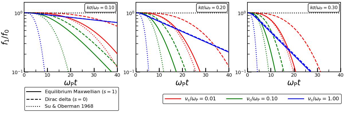
Figure 1: The continuum response of a weakly collisional plasma as a function of time for three different values of $\nu_{\rm c}$ indicated by the red, green and blue lines, and three different values of $k\sigma$ in the three panels. The solid lines indicate the response when the initial perturbation in the DF is of the equilibrium Maxwellian form ($s=\sigma_{0}/\sigma=1$). The dashed lines denote the response for an initial perturbation that is Dirac delta in the velocities ($s=0$). The dotted lines indicate the continuum response predicted by [11]. Note that the $s=1$ and $s=0$ cases are very similar for $\nu_{\rm c}>k\sigma$, but different, albeit with the same temporal scaling, otherwise. The continuum response decays as $\sim\exp{\left[-{\left(k\sigma\right)}^{2}\nu_{\rm c}t^{3}/3\right]}$ for the $s=1$ case and $\sim\exp{\left[-{\left(k\sigma\right)}^{2}\nu_{\rm c}t^{3}/12\right]}$ for the $s=0$ case at $t<1/\nu_{\rm c}$, but switches over to a much slower $\sim\exp{\left[-\left({\left(k\sigma\right)}^{2}/\nu_{\rm c}\right)t\right]}$ decay at $t>1/\nu_{\rm c}$, unlike [11] who only predict the former super-exponential decay. Note that the collisional damping is most pronounced for $\nu_{\rm c}\sim k\sigma$, or in other words, when the perturbation scale, $\lambda\sim 1/k$, is comparable to the mean free path of collisions, $\lambda_{\rm c}=\sigma/\nu_{\rm c}$.

IV.1 Different models for $h_{\kappa}(u)$

Evidently, the temporal behaviour of the continuum response depends on the functional form of the initial perturbation, $h_{\kappa}(u)$. We compute the response for a few specific models of $h_{\kappa}(u)$.

IV.1.1 Gaussian pulse

Let us consider the case of an initial perturbation in the DF that is Gaussian or Maxwellian in velocities, but with a velocity dispersion different from the equilibrium velocity dispersion $\sigma$:

$$h_{\kappa}(u)=\frac{h_{\kappa 0}}{\sqrt{2\pi s^{2}}}\exp{\left[-\frac{{\left(u-u_{0}\right)}^{2}}{2s^{2}}\right]}.$$ (21)

Here, $u_{0}$ is the drift velocity of the initial pulse, and $\sigma_{0}$ is its velocity dispersion, with $s=\sigma_{0}/\sigma$. The velocity Fourier transform of $h_{\kappa}(u)$ is given by

$$H_{\kappa}(w)=\frac{h_{\kappa 0}}{2\pi}\exp{\left[-\frac{s^{2}w^{2}}{2}-iu_{0}w\right]}.$$ (22)

In this case, the continuum response in equation (19) becomes

$$g_{1\kappa}^{\rm cont}(u,t) =\frac{h_{\kappa 0}}{\sqrt{2\pi\delta^{2}_{u}(t)}}\exp{\left[-\frac{{\left(u-u_{0}e^{-\nu_{\rm c}t}\right)}^{2}}{2\delta^{2}_{u}(t)}\right]}$$

$$\times\exp{\left[-\kappa^{2}\delta^{2}_{x}(t)\right]}\times\exp{\left[-i\kappa\left(\zeta^{(1)}_{x}(t)u+\zeta^{(2)}_{x}(t)u_{0}\right)\right]},$$ (23)

where

$$\zeta_{x}^{(1)}(t)=\frac{\left(1-e^{-\nu_{\rm c}t}\right)\left(1-\left(1-s^{2}\right)e^{-\nu_{\rm c}t}\right)}{1-\left(1-s^{2}\right)e^{-2\nu_{\rm c}t}},$$

$$\zeta_{x}^{(2)}(t)=\frac{{\left(1-e^{-\nu_{\rm c}t}\right)}^{2}}{1-\left(1-s^{2}\right)e^{-2\nu_{\rm c}t}},$$

$$\delta^{2}_{u}(t)=1-\left(1-s^{2}\right)e^{-2\nu_{\rm c}t},$$

$$\delta^{2}_{x}(t)=\nu_{\rm c}t-\frac{1-e^{-\nu_{\rm c}t}}{2}\frac{3-e^{-\nu_{\rm c}t}+\left(1-s^{2}\right)\left(1-3e^{-\nu_{\rm c}t}\right)}{1-\left(1-s^{2}\right)e^{-2\nu_{\rm c}t}}.$$ (24)

Let us analyze separately the key features of the above response. The first factor in equation (23) denotes the damping and broadening of the initial perturbation in the velocity space due to the collisional diffusion of particle velocities. The perturbation starts out being a Gaussian (in $u$) with a velocity dispersion $s$ (in units of $\sigma$), then gradually damps away and spreads out to attain the equilibrium Maxwellian form with velocity dispersion $\sigma$.

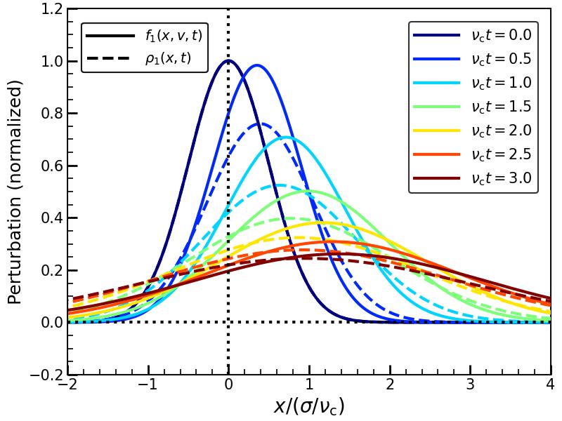
Figure 2: The continuum response of a weakly collisional plasma as a function of $x$ (in units of $\sigma/\nu_{\rm c}$). The solid lines denote $f_{1}(x,v,t)$ (computed using equation [26] and normalized by its maximum value at $t=0$) at seven different values of $\nu_{\rm c}t$ as indicated, while the dashed lines denote $\rho_{1}(x,t)$ (computed using equation [27] and normalized by its maximum value at $t=0$). We adopt $\sigma_{x,0}=0.5\sigma/\nu_{\rm c}$, $v=0.5\sigma$, $v_{0}=\sigma$ and $s=\sigma_{0}/\sigma=0.9$, i.e., the initial DF perturbation is close to the equilibrium Maxwellian form. Both quantities have been normalized by their maximum value at $t=0$. Note that both perturbations decay, broaden and slow down in $x$ due to collisional diffusion followed by damping, but the density perturbation decays faster due to the additional effect of phase-mixing.

The second factor in equation (23) indicates the damping of the response (in $\kappa$) due to collisions. The extent of damping depends on the wave-number $k$ of the perturbation. The asymptotic temporal behaviour of this damping factor for the $s\neq 0$ case (we shall discuss the $s=0$ case, which corresponds to an initial Dirac delta pulse, separately) is as follows:

$$\exp{\left[-\kappa^{2}\delta^{2}_{x}(t)\right]}\approx\begin{cases}\exp{\left[-\kappa^{2}{\left(\nu_{\rm c}t\right)}^{3}/3\right]}=\exp{\left[-{\left(k\sigma\right)}^{2}\nu_{\rm c}t^{3}/3\right]},\;\;\;\;\;\;\;\,\nu_{\rm c}t\ll 1,\\ \exp{\left[-\kappa^{2}\nu_{\rm c}t\right]}=\exp{\left[-\left({\left(k\sigma\right)}^{2}/\nu_{\rm c}\right)t\right]},\;\;\;\;\;\;\;\;\;\;\;\;\;\;\nu_{\rm c}t\gg 1.\end{cases}$$ (25)

The small time ($t\ll 1/\nu_{\rm c}$) behaviour of the above collisional damping factor is similar to the classic [11] result. This damping occurs super-exponentially over a timescale, $\tau_{{\rm d},1}={\left(3/\nu_{\rm c}{\left(k\sigma\right)}^{2}\right)}^{1/3}$. However, the long time ($t\gg 1/\nu_{\rm c}$) damping occurs exponentially, much slower than the [11] prediction. The timescale of this late time decay is $\tau_{{\rm d},2}=\nu_{\rm c}/{\left(k\sigma\right)}^{2}$. When $\nu_{\rm c}\sim k\sigma$, or in other words the scale of the perturbation, $\lambda\sim 1/k$, is comparable to the mean free path, $\lambda_{\rm c}=\sigma/\nu_{\rm c}$, $\tau_{{\rm d},1}$ is comparable to $\tau_{{\rm d},2}$, and the corresponding response damps the most. This is evident in Fig. 1, which plots the amplitude of the continuum response as a function of time for six different values of $\nu_{\rm c}$ and three different values of $k\sigma$ as indicated. Our result, computed using equation [23], is shown by the solid and dashed lines for the $s=1$ and $0$ cases respectively, and the corresponding [11] prediction is shown by dotted lines. The remarkable difference between our prediction and that of [11] is a consequence of the fact that they neglected the damping/drag term in the LB operator, i.e., the first term on the RHS of equation (8). This approximation is justified only for $t\lesssim 1/\nu_{\rm c}$, when collisions cause the particle velocities to diffuse/disperse rather than damp on an average. This is the diffusive regime of collisions. However, collisions not only disperse the velocities of the particles but also damp out their individual mean velocities over time. This damping regime, which takes over at $t\gtrsim 1/\nu_{\rm c}$, is described by the first term on the RHS of equation (8), the very term that [11] neglect. By neglecting the damping term, [11] have limited themselves to the diffusive regime of collisions, and therefore missed out on the crucial switchover of the decay to a slow exponential one in the long time damping regime. To obtain more physical insight into this, we shall discuss the collisional dynamics in the diffusive and damping regimes in detail, in section IV.2, using a stochastic analysis with the Langevin equation, which is complementary to the Fokker-Planck approach taken so far.

The third factor in equation (23) is a phase factor that denotes the free streaming of the particles. It can be seen that at small time ($\nu_{\rm c}t\ll 1$), this factor evolves as $\exp{\left[-i\kappa u\nu_{\rm c}t\right]}=\exp{\left[-ikvt\right]}$. This behaviour is the same as that in the collisionless ($\nu_{\rm c}\to 0$) case. At large time ($\nu_{\rm c}t\gg 1$), the phase factor becomes $\exp{\left[-i\kappa\left(u+u_{0}\right)\right]}$, and therefore time-independent. This implies that the pulse comes to a halt after roughly the collision time, $1/\nu_{\rm c}$, owing to the constant drainage of linear momentum from a particle via collisions. This is a generic feature of collisional damping in Fokker-Planck dynamics.

So far we have seen that each $k$ mode of the continuum response damps away and decelerates due to collisional diffusion and damping. The spatial response is an integrated response of all $k$ modes. Since each $k$ mode damps away at a rate that depends non-linearly on $k$, the spatial response, which is the sum of all $k$ modes, will deviate from its initial functional form over time, i.e., the weakly collisional plasma acts as a dispersive medium. We shall demonstrate this by computing the spatial response for a given spatial distribution of the initial perturbation, i.e., a given $h_{\kappa 0}$. Since the response for each $k$ mode is Gaussian in $k$, as evident from equation (23) (for a Gaussian velocity distribution of the initial perturbation as we consider here), the integration over $k$ is straightforward for a Gaussian (in $k$) functional form of $h_{\kappa 0}$, i.e., a Gaussian (in $x$) functional form of the initial perturbation. The spatial response can be obtained by taking the inverse spatial Fourier transform of equation (23). For an initial Gaussian pulse with spatial dispersion $\sigma_{x,0}$, i.e., $g_{1}(x,u,0)=\left(F/{\sqrt{2\pi}}\right)\exp{\left[-x^{2}/2\sigma^{2}_{x,0}\right]}\,\exp{\left[-{\left(u-u_{0}\right)}^{2}/2s^{2}\right]}$, for which $h_{\kappa 0}=\left(F/2\pi\right)\exp{\left[-k^{2}\sigma^{2}_{x,0}/2\right]}\,\exp{\left[-{\left(u-u_{0}\right)}^{2}/2s^{2}\right]}$, we take the inverse Fourier transform of equation (23) and re-establish the dimensions to obtain the following form for the response:

$$f_{1}^{\rm cont}(x,v,t)=\frac{n_{e}}{\sigma}\int_{-\infty}^{\infty}{\rm d}k\,\exp{\left[ikx\right]}\,g_{1\kappa}^{\rm cont}(u,t)$$

$$=\frac{n_{e}F}{\sqrt{2\pi\sigma^{2}\delta^{2}_{u}(t)}}\exp{\left[-\frac{{\left(v-v_{0}e^{-\nu_{\rm c}t}\right)}^{2}}{2\sigma^{2}\delta^{2}_{u}(t)}\right]}\times\frac{1}{\sqrt{2\pi\left(\sigma^{2}_{x,0}+2{\left(\sigma/\nu_{\rm c}\right)}^{2}\delta^{2}_{x}(t)\right)}}\exp{\left[-\frac{{\left[x-\frac{1}{\nu_{\rm c}}\left(\zeta_{x}^{(1)}(t)v+\zeta_{x}^{(2)}(t)v_{0}\right)\right]}^{2}}{{2\left(\sigma^{2}_{x,0}+2\left(\sigma/\nu_{\rm c}\right)^{2}\delta^{2}_{x}(t)\right)}}\right]}.$$ (26)

Conservation of particle number ensures that the pulse damps out as well as broadens due to collisions, as manifested by both $x$ and $v$ parts of the above response. The spatial broadening of the pulse occurs as $\sim\left(2\sigma^{2}/3\nu_{\rm c}^{2}\right){\left(\nu_{\rm c}t\right)}^{3}$ for $t\lesssim 1/\nu_{\rm c}$, and as $\sim\left(2\sigma^{2}/\nu_{\rm c}^{2}\right)\nu_{\rm c}t$ for $t\gtrsim 1/\nu_{\rm c}$, while the spatial damping occurs as the inverse of this. If the width of the initial pulse is small, i.e., $\sigma_{x,0}\ll\sigma/\nu_{\rm c}$, it damps and broadens in the former way for a long time, i.e., we are in the diffusive regime. The typical damping timescale in this regime is $\sim{\left(3\sigma^{2}_{x,0}/2\sigma^{2}\nu_{\rm c}\right)}^{1/3}$. On the other hand, a well-extended initial pulse with $\sigma_{x,0}\gg\sigma/\nu_{\rm c}$, falls in the damping regime, i.e., it quickly transitions to the latter phase of exponential damping and broadening, which occurs over a relatively long timescale of $\sim\left(\sigma^{2}_{x,0}/2\sigma^{2}\right)\nu_{\rm c}$. Since both timescales increase with $\sigma_{x,0}$ (for fixed $\nu_{\rm c}$ and $\sigma$), we see that small scale perturbations collisionally damp away faster than large scale ones. Moreover, since the former timescale decreases with $\nu_{\rm c}$ (for fixed $\sigma_{x,0}$ and $\sigma$) and the latter increases, perturbations damp slowly in both small and large $\nu_{\rm c}$ limits. The damping and broadening of the pulse due to collisions is visible in Fig. 2, which plots $f_{1}$ (solid lines) as a function of $x$ at different points of time as indicated. Note that the pulse slows down over time due to collisional damping. The three key features of Fokker-Planck collisional dynamics are the damping, broadening and deceleration of a pulse, all three of which are manifest in Fig. 2.

Let us now study the evolution of the density perturbation, $\rho_{1}^{\rm cont}(x,t)=\int{\rm d}v\,f_{1}^{\rm cont}(x,v,t)$. Upon integrating equation (26) over velocity, we obtain

$$\rho_{1}^{\rm cont}(x,t)$$

$$=\frac{n_{e}F}{\sqrt{2\pi\left[\sigma^{2}_{x,0}+{\left(\frac{\sigma}{\nu_{\rm c}}\right)}^{2}\left\{2\delta^{2}_{x}(t)+{\zeta^{(1)}_{x}}^{2}(t)\,\delta^{2}_{u}(t)\right\}\right]}}$$

$$\times\exp{\left[-\frac{{\left(x-\frac{v_{0}}{\nu_{\rm c}}\left(1-e^{-\nu_{\rm c}t}\right)\right)}^{2}}{2\left[\sigma^{2}_{x,0}+{\left(\frac{\sigma}{\nu_{\rm c}}\right)}^{2}\left\{2\delta^{2}_{x}(t)+{\zeta^{(1)}_{x}}^{2}(t)\,\delta^{2}_{u}(t)\right\}\right]}\right]}.$$ (27)

The density perturbation initially propagates at velocity $v_{0}$ and comes to a halt after $t\sim 1/\nu_{\rm c}$. At the same time, it damps and spreads out. This is not only due to collisional damping but also phase-mixing, as long as the initial perturbation has some finite spread in velocities, or in other words particles are initially perturbed over a finite velocity range. The width of the Gaussian scales as $\sim\sqrt{\sigma^{2}_{x,0}+\sigma^{2}t^{2}}$ at small $t$, due to phase-mixing. At intermediate time, the width scales as $\sim\sqrt{\sigma^{2}_{x,0}+\sigma^{2}\nu_{\rm c}t^{3}/3}$, which is an outcome of the collisional diffusion of particle velocities. At late time, it scales as $\sim\sqrt{\sigma^{2}_{x,0}+2\left(\sigma^{2}/\nu_{\rm c}\right)t}$, due to collisional damping. Due to the additional contribution of phase-mixing to the damping besides collisions, the density perturbation $\rho^{\rm cont}_{1}$ damps away faster than the fine-grained DF $f^{\rm cont}_{1}$, as manifest in Fig. 2 that plots $f^{\rm cont}_{1}$ (solid lines) and $\rho^{\rm cont}_{1}$ (dashed lines) as functions of $x$.

IV.1.2 Dirac delta pulse

We now evaluate the response in the $s\to 0$ limit of the initial Gaussian pulse. This corresponds to an initial pulse that is Dirac delta in the particle velocities, i.e., $h_{\kappa}(u)=h_{\kappa 0}\delta(u-u_{0})$, whose Fourier transform is $H_{\kappa}(w)=h_{\kappa 0}\exp{\left[-iu_{0}w\right]}/(2\pi)$. In this case, the response is given by equation (23), with

$$\zeta_{x}^{(1)}(t)=\zeta_{x}^{(2)}(t)=\tanh{\frac{\nu_{\rm c}t}{2}},$$

$$\delta^{2}_{u}(t)=1-e^{-2\nu_{\rm c}t},$$

$$\delta^{2}_{x}(t)=\nu_{\rm c}t-2\tanh{\frac{\nu_{\rm c}t}{2}}.$$ (28)

The asymptotic temporal behaviour of the collisional damping factor is:

$$\exp{\left[-\kappa^{2}\delta^{2}_{x}(t)\right]}\approx\begin{cases}\exp{\left[-\kappa^{2}{\left(\nu_{\rm c}t\right)}^{3}/12\right]}=\exp{\left[-{\left(k\sigma\right)}^{2}\nu_{\rm c}t^{3}/12\right]},\;\;\;\nu_{\rm c}t\ll 1\\ \exp{\left[-\kappa^{2}\nu_{\rm c}t\right]}=\exp{\left[-\left({\left(k\sigma\right)}^{2}/\nu_{\rm c}\right)t\right]},\;\;\;\;\;\;\;\;\;\;\;\;\;\nu_{\rm c}t\gg 1.\end{cases}$$ (29)

Note that the small time behaviour of the damping is the same as that in the general case given by equation (25), expect for the numerical factor of the exponent. The long time behaviour is exactly the same as equation (25).

The phase factor, $\exp{\left[-i\kappa(\zeta^{(1)})_{x}(t)u+\zeta^{(2)})_{x}(t)u_{0}\right]}$, scales as $\sim\exp{\left[-i\kappa(u+u_{0})t/2\right]}=\exp{\left[-ik(v+v_{0})t/2\right]}$ for $\nu_{\rm c}t\to 0$. In this limit, the velocity part of the response tends to $\delta(v-v_{0})$, and thus the phase-factor goes to $\exp{\left[-ikvt\right]}$. This reproduces the form of the continuum response in the collisionless limit.

IV.1.3 Equilibrium Gaussian pulse

In the $s\to 1$ limit, the initial perturbation, $h_{\kappa}(u)$, is of the equilibrium Maxwellian form, i.e., $h_{\kappa}(u)=h_{\kappa 0}\exp{\left[-{\left(u-u_{0}\right)}^{2}/2\right]}/\sqrt{2\pi}$, and its Fourier transform is equal to $H_{\kappa}(w)=h_{\kappa 0}\exp{\left[-w^{2}/2-iu_{0}w\right]}/(2\pi)$. In this case, the response is given by equation (23), with

$$\zeta_{x}^{(1)}(t)=1-e^{-\nu_{\rm c}t},$$

$$\zeta_{x}^{(2)}(t)={\left(1-e^{-\nu_{\rm c}t}\right)}^{2},$$

$$\delta_{u}(t)=1,$$

$$\delta^{2}_{x}(t)=\nu_{\rm c}t-\frac{\left(1-e^{-\nu_{\rm c}t}\right)\left(3-e^{-\nu_{\rm c}t}\right)}{2}.$$ (30)

The phase factor is $\exp{\left[-ik\left(1-e^{-\nu_{\rm c}t}\right)\left(v+v_{0}\left(1-e^{-\nu_{\rm c}t}\right)\right)\right]}$, which scales as $\exp{\left[-ikvt\right]}$ in the $\nu_{\rm c}t\to 0$ limit. This recovers the form of the continuum response in the limit of zero collisions. The perturbation is initially of the equilibrium Maxwellian form and therefore remains so throughout, since the Maxwellian DF is an equilibrium solution of the Boltzmann-Poisson equations with the LB collision operator. The amplitude of the response, however, damps away due to collisional diffusion and damping. The damping factor has the same asymptotic behaviour as in the general case given by equation (25), i.e., the response damps away super-exponentially till $t\sim 1/\nu_{\rm c}$ and transitions to a slower exponential decay afterwards.

IV.2 Langevin approach: diffusive and friction regimes

So far, we have seen that the collisional relaxation of a plasma occurs in two distinct regimes: the diffusive and friction regimes. The nature of relaxation in these two regimes is very different. These distinct behaviours of plasma relaxation can be understood by taking a closer look at the stochastic dynamics of collisions. We assume that the collisions are typically short-range random encounters, and therefore mimic a stochastic process that changes the phase space coordinates of the particles. If the collisions are random enough, they erase the dynamical memory (initial conditions) of the colliding particles over time, i.e., the collisional scatterings can be thought of as Markovian random walks of the particles in phase space. A key consequence of this random (or chaotic) nature of collisions is the phenomenon of molecular chaos, which refers to the fact that the momenta of two colliding particles, despite being correlated immediately after a collision, become uncorrelated soon enough due to their encounters with other particles. This justifies the use of the Boltzmann equation as the governing kinetic equation. This also ensures that the collisions are approximately uncorrelated in time and can be modelled by a stochastic acceleration with a white noise power spectrum. Hence, in the same spirit as that of modeling Brownian motion [15, 16], we can model the collisional dynamics in a plasma using the Langevin equation, which is nothing but Newton’s equation of motion with damping and stochastic forces:

$$\frac{{\rm d}^{2}x}{{\rm d}t^{2}}+\nu_{\rm c}\frac{{\rm d}x}{{\rm d}t}=\xi(t).$$ (31)

Here, $-\nu_{\rm c}{\rm d}x/{\rm d}t$ is the collisional damping/deceleration, also known as friction, and $\xi(t)$ is the stochastic acceleration due to collisions. We assume that $\xi(t)$ has a zero ensemble average and a white noise or uncorrelated power spectrum, i.e.,

$$\left<\xi(t)\right>=0,$$

$$\left<\xi(t)\,\xi(t^{\prime})\right>={\cal D}\,\delta(t-t^{\prime}),$$ (32)

where ${\cal D}$ is a constant with the dimensions of velocity squared per unit time.

The Langevin equation is a stochastic differential equation which evolves the trajectory of each individual particle. The ensemble averages of the evolving phase space quantities and their dispersions, obtained by solving the Langevin equation, are the same as the first and second moments of these quantities, obtained with respect to the DF that evolves via the Fokker-Planck equation, as long as the initial DF perturbation is sufficiently close to the equilibrium Maxwellian form. In fact the Fokker-Planck collision operator corresponding to the Langevin equation given in equation (31) is the LB operator. The correspondence between the Langevin and Fokker-Planck equations therefore justifies that the results obtained in this section are an alternative way to obtain the various scalings of the response that are computed using the Fokker-Planck (LB) equation in the previous sections.

Before solving the Langevin equation in its full glory, let us first take a careful look at the applicability of this equation in modeling plasma collisions. The key assumption is that the collisions can be modelled as short-range random encounters, despite the fact that Coulomb interactions between charged particles are long-range. The impact parameter of effective collisions is typically the Debye length, making the collisions functionally short-range. Hence, as long as collisional relaxation is dominated by scales larger than the Debye length ($\omega_{\rm P}\gtrsim k\sigma$), as is typically the case for a weakly collisional plasma, the collisions can be modelled as short-range stochastic encounters, and the Langevin (equivalently, the Fokker-Planck) description in this paper should properly capture the essential physics of plasma collisions.

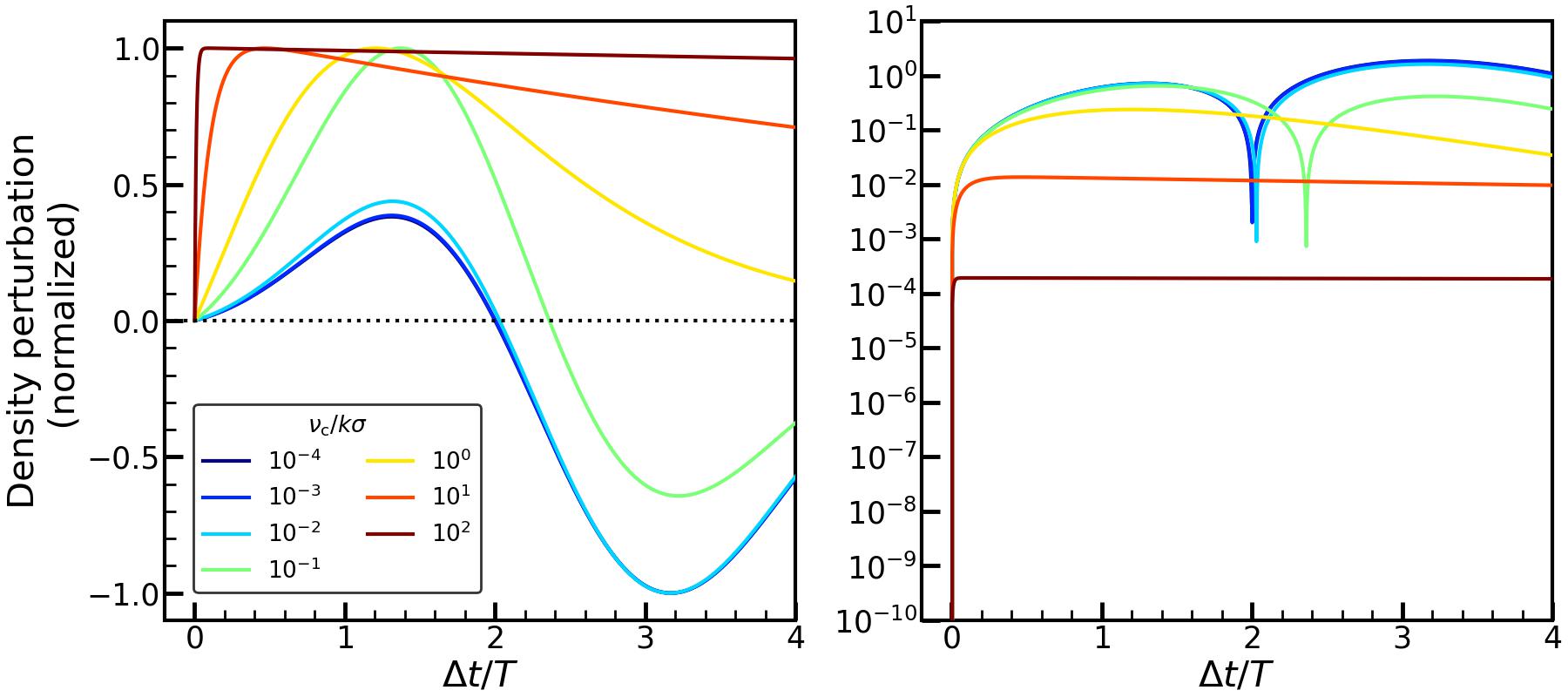
(a) $k\sigma T=1$

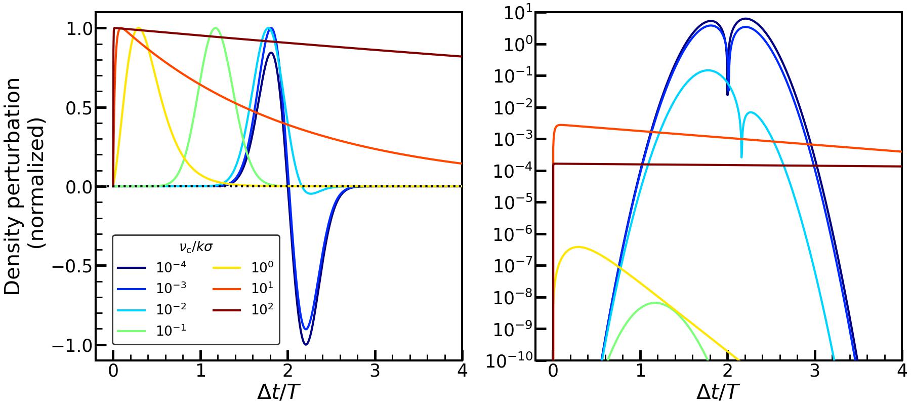
(b) $k\sigma T=5$

Figure 3: Plasma echo: Second order density perturbation of the $k=\left(k_{1}-k_{2}\right)$ mode as a function of $\Delta t/T$, with $\Delta t=t-T$ the time elapsed since the second pulse is introduced at $T$ (see Appendix C and section IV.3 for details). The first and second pulses have wavenumbers $k_{1}$ and $k_{2}$ respectively. Here we have adopted $k_{1}\sigma/\nu_{\rm c}=3$ and $k_{2}\sigma/\nu_{\rm c}=2$. The top and bottom panels correspond to $k\sigma T=1$ and $5$ respectively. The left panel indicates the density perturbation, $r_{2\kappa}$, normalized by its maximum absolute value, and the right panel indicates $r_{2\kappa}/\left(ab\left(k_{1}\sigma t_{\rm P}\right)\left(k_{2}\sigma t_{\rm P}\right)\right)$, where $a$ and $b$ are the dimensionless strengths of the first and second potential pulses respectively, and $t_{\rm P}$ is the temporal pulsewidth that goes to zero, keeping $at_{\rm P}$ and $bt_{\rm P}$ finite. The spikes in the density perturbation indicate the echos. These occur at $\Delta t/T\approx k_{2}/\left(k_{1}-k_{2}\right)=2$ in the collisionless limit. The echo time approaches $T$ with increasing $\nu_{\rm c}$. Note that the echoes are detectable even for $\nu_{\rm c}/k\sigma\sim 1$, as long as $k\sigma T$ is small, i.e., the initial response has not sufficiently decayed via phase-mixing.

With the aforementioned assumptions, let us now solve the Langevin equation to evaluate the mean trajectories of particles and the position and velocity dispersions around them. Integrating equation (31) once with respect to $t$, with the initial condition, $v(0)=v_{0}$, we obtain the following form for the velocity:

$$v(t)=\frac{{\rm d}x}{{\rm d}t}=v_{0}\,e^{-\nu_{\rm c}t}+\int_{0}^{t}{\rm d}t^{\prime}\,e^{-\nu_{\rm c}(t-t^{\prime})}\xi(t^{\prime}).$$ (33)

Since the ensemble average of $\xi(t)$ is zero, the ensemble averaged or mean velocity is equal to

$$\left<v(t)\right>=v_{0}\,e^{-\nu_{\rm c}t}.$$ (34)

The exponential decay of the mean velocity manifests damping or friction: the constant drainage of momentum from each particle due to collisions.

The velocity dispersion is given by (see Appendix B for detailed derivation)

$$\sigma^{2}(t) =\left<\left(v(t)-v_{0}\,e^{-\nu_{\rm c}t}\right)^{2}\right>$$

$$=\frac{{\cal D}}{\nu_{\rm c}}\left(1-e^{-2\nu_{\rm c}t}\right),$$ (35)

where we have used the uncorrelated nature of the stochastic force, i.e., the second of equations (32). Note that the velocity dispersion initially increases linearly with time, i.e., $\sigma^{2}(t)\sim 2{\cal D}\,t$. This is the essence of velocity diffusion or particle random walk in the velocity space, and is caused by the stochastic acceleration, $\xi(t)$. The late-time dynamics, which sets in after $t\sim 1/\nu_{\rm c}$, is governed by the frictional deceleration, $-\nu_{\rm c}{\rm d}x/{\rm d}t$. This friction/damping drives $\sigma^{2}$ towards the equilibrium value, $\lim_{t\to\infty}\sigma^{2}(t)=\sigma^{2}$. Thus, from the above equation, we infer that ${\cal D}=\nu_{\rm c}\sigma^{2}$. This is nothing but the celebrated Einstein relation. ${\cal D}$ is the velocity diffusion coefficient, which is related to the damping coefficient or collision frequency, $\nu_{\rm c}$, by the proportionality factor, $\sigma^{2}$. Therefore, friction and diffusion go hand-in-hand during collisions, and one cannot exist without the other. Consequently, neglecting the friction term in the collision operator [11, 12, etc.] is bound to provide an incomplete description of collisional dynamics, which may lead to erroneous conclusions about the long time decay of the response in weakly collisional plasmas.

Let us now evaluate the time dependence of the particle position. Integrating equation (33) with respect to $t$, with the initial condition that $x(0)=0$, we obtain

$$x(t) =\frac{v_{0}}{\nu_{\rm c}}\left(1-e^{-\nu_{\rm c}t}\right)+\int_{0}^{t}{\rm d}t^{\prime}\int_{0}^{t^{\prime}}{\rm d}t^{\prime\prime}\,e^{-\nu_{\rm c}\left(t^{\prime}-t^{\prime\prime}\right)}\xi(t^{\prime\prime}).$$ (36)

Recalling that $\left<\xi(t)\right>=0$, we see that the mean position is equal to

$$\left<x(t)\right>=\frac{v_{0}}{\nu_{\rm c}}\left(1-e^{-\nu_{\rm c}t}\right),$$ (37)

i.e., the particle gradually slows down and traverses an overall distance of $v_{0}/\nu_{\rm c}$. The mean-squared position is given by (see Appendix B for detailed derivation)

$$\sigma^{2}_{x}(t) =\left<{\left[x(t)-\frac{v_{0}}{\nu_{\rm c}}\left(1-e^{-\nu_{\rm c}t}\right)\right]}^{2}\right>$$

$$={\left(\frac{\sigma}{\nu_{\rm c}}\right)}^{2}\left[\nu_{\rm c}t-\frac{\left(1-e^{-\nu_{\rm c}t}\right)\left(3-e^{-\nu_{\rm c}t}\right)}{2}\right],$$ (38)

where we have used the second of equations (32), i.e., $\xi(t)$ is a white noise source. Initially, in the diffusive regime, where the dynamics is predominantly driven by the stochastic acceleration $\xi(t)$, the mean-squared position scales as $\sigma^{2}_{x}(t)\sim\nu_{\rm c}\sigma^{2}t^{3}/3$. This is a consequence of the fact that the velocity dispersion, $\sigma^{2}\approx{\rm d}^{2}\sigma^{2}_{x}/{\rm d}t^{2}$, scales as $\sim 2{\cal D}\,t=2\sigma^{2}\nu_{\rm c}t$ in this regime. Finally, after $t\sim 1/\nu_{\rm c}$, the mean-squared position scales as $\sigma^{2}_{x}(t)\sim(\sigma^{2}/\nu_{\rm c})\,t$. This owes to the fact that the velocity dispersion, $\sigma^{2}(t)\approx\nu_{\rm c}\,{\rm d}\sigma^{2}_{x}/{\rm d}t$, attains a nearly constant value, $\sigma^{2}$, due to friction. In this late-time friction-dominated regime, the velocity evolution is governed by the frictional deceleration, but the evolution of the mean-squared position is still driven by the stochastic acceleration, $\xi(t)$.

The temporal dependence of the mean and mean squared velocity and position obtained from the above analysis is very similar to what shows up in our analysis of plasma relaxation using the LB operator in the previous sections. The exponentially decaying drift velocity obtained from the Langevin analysis (equation [34]), is the same as the drift velocity of the pulse obtained using the LB analysis (see equations [23] and 26). The slowing drift of the mean position is manifest in both the Langevin (equation [37]) and LB (equation [27]) analyses. The time-dependence of the velocity dispersion is also the same; compare $\sigma^{2}(t)$ in equation (35) with $\sigma^{2}\delta^{2}_{u}(t)$ in equation (26), where $\delta^{2}_{u}(t)$ is given by the second of equations (28). And the mean squared position, computed using the Langevin equation (equation [38]) is the same as the spatial width of the response computed using the LB analysis (note $\delta^{2}_{x}(t)$ in equation [30]). The prefactors of the above quantities slightly differ between the LB and Langevin analyses when the initial perturbation in the DF is very different from the equilibrium Maxwellian form. This is because the diffusion coefficients of the LB operator rely on the Einstein relation, and are therefore dictated by the equilibrium Maxwellian DF. The correspondence is exact only when the initial pulse is of the equilibrium Maxwellian form in velocities. Still, the asymptotic temporal behaviour of $\left<x\right>$, $\left<v\right>$, $\sigma^{2}_{x}$ and $\sigma^{2}$ obtained using the Langevin analysis is the same as that obtained using the LB analysis in all cases. This proves that the LB operator, despite being only an approximate description of collisional dynamics, properly captures the essential physics of collisions, particularly in the small and large time limits. Put differently, the diffusive and friction regimes of collisional relaxation predicted by the LB operator in section IV.1 are not merely artefacts of the form of the collision operator chosen, but are qualitatively robust phenomena in a system governed by weak collisions.

IV.3 Implications for the plasma echo

The key features of the continuum response in a weakly collisional plasma are: (i) it decays super-exponentially with time for $\lambda<\lambda_{\rm c}$ but exponentially for $\lambda>\lambda_{\rm c}$, and gets damped the most for $\lambda\sim\lambda_{\rm c}$, and (ii) an externally imposed pulse slows down over time due to the collisional damping of particle velocities over a collision time, $1/\nu_{\rm c}$. These behaviors not only impact the linear regime of plasma relaxation, but also have implications for the survival and persistence of coherent structures and non-linear phenomena. One such non-linear phenomenon is the plasma echo [17, 11, 18, 19], which attests to the time-reversibility of the Vlasov equation and arises from the continuum response. The fine-grained continuum response to a perturbation gives rise to a macroscopic disturbance, when a second perturbation is introduced into the system sometime after the first perturbation and interferes with the response to it.

Let us analyze the echo problem in some detail, and understand the impact of collisionality on this phenomenon. This requires us to evaluate the second order response of the plasma to an external perturbation. Since we are interested in the echo phenomenon, which is caused by the continuum response, we ignore the self-potentials $\Phi_{1}$ and $\Phi_{2}$ in this section. We assume that the plasma is excited at $t=0$ by an impulsive kick of sinusoidal electric field with wavenumber $k_{1}$. The plasma is impulsively kicked for a second time at $t=T$ by another sinusoidal electric field with wavenumber $k_{2}$. The corresponding $k$ Fourier mode of the potential is given by (see Appendix C for details)

$$\tilde{\Phi}_{k}(\gamma)=t_{\rm P}\left[A\,\delta\left(k-k_{1}\right)\delta(t)+B\left(k+k_{2}\right)\delta(t-T)\right],$$ (39)

where $A$ and $B$ are constants, and $t_{\rm P}$ is the temporal pulsewidth that goes to zero, keeping $At_{\rm P}$ and $Bt_{\rm P}$ finite. The resulting second order response, $g_{2\kappa}=\left(\sigma/n_{e}\right)f_{2k}$ (derived in detail in Appendix C), is given by equations (86) and (85). The third term in equation (86) is the relevant term for the plasma echo. It denotes a response at the wavenumber, $k=k_{1}-k_{2}$, which manifests the echo born out of the interference between the first and second pulses. The phase-factor in this term scales as $\sim\exp{\left[-i\frac{v}{\nu_{\rm c}}\left(\left(k_{1}-k_{2}\right)\left(1-e^{-\nu_{\rm c}\left(t-T\right)}\right)-k_{2}e^{-\nu_{\rm c}\left(t-T\right)}\left(1-e^{-\nu_{\rm c}T}\right)\right)\right]}$, which becomes independent of $v$ when the argument is zero. This corresponds to a bunching of particles and an enhancement in the macroscopic density perturbation: the echo. It occurs at

$$t=t_{\rm echo}\approx T+\frac{1}{\nu_{\rm c}}\ln\left|1+\frac{k_{2}}{k_{1}-k_{2}}\left(1-e^{-\nu_{\rm c}T}\right)\right|.$$ (40)

The approximation improves in accuracy for large $\left(k_{1}-k_{2}\right)\sigma T$. In the collisionless ($\nu_{\rm c}T\to 0$) limit, the phase-factor scales as $\sim\exp{\left[-iv\left(\left(k_{1}-k_{2}\right)t-k_{1}T\right)\right]}$. Accordingly, the echo occurs at $t_{\rm echo}\approx k_{1}T/\left(k_{1}-k_{2}\right)$, which is also the $\nu_{\rm c}T\to 0$ limit of equation (40). This is the classic result for echo formation in a collisionless plasma [17]. In the strong collision ($\nu_{\rm c}T\to\infty$) limit, $t_{\rm echo}\approx T+\frac{1}{\nu_{\rm c}}\ln{\left|k_{1}/\left(k_{1}-k_{2}\right)\right|}$. Hence, the echo forms closer to $T$, the time of the second pulse, and becomes increasingly difficult to detect with increasing $\nu_{\rm c}$.

The echo involves the continuum response becoming independent of $v$, and therefore corresponds to a macroscopic disturbance in the plasma density. Keeping this in mind, the $\left(k_{1}-k_{2}\right)$ mode of the second order density perturbation, $r_{2\kappa}=\rho_{2k}/\rho_{0}$, is computed in Appendix C by integrating the cross term of the second order response, $g_{2\kappa}$ (given in equation [86), over $u$, and is given by equation (88). The left panels of Fig. 3 plot $r_{2\kappa}$, divided by its maximum absolute value, as a function of $\Delta t/T=\left(t-T\right)/T$. The right panels plot the absolute value of $r_{2\kappa}/\left(ab\left(k_{1}\sigma t_{\rm P}\right)\left(k_{2}\sigma t_{\rm P}\right)\right)$ as a function of $\Delta t/T$. Here $a$ and $b$ are the dimensionless strengths of the first and second potential pulses respectively (see Appendix C for details). The top and bottom panels correspond to $\left(k_{1}-k_{2}\right)\sigma T=1$ and $5$ respectively. We adopt $k_{1}\sigma/\nu_{\rm c}=3$ and $k_{2}\sigma/\nu_{\rm c}=2$. The spikes in the density perturbation are the echoes. In the collisionless limit, the echoes occur at times close to $\Delta t/T\approx k_{2}/\left(k_{1}-k_{2}\right)=2$. The time of the echo approaches $T$ with increasing $\nu_{\rm c}$, which is also evident from equation (40), and becomes indistinguishable from $T$ in the $\nu_{\rm c}T\to\infty$ limit. The right panels of Fig. 3 show that the response gets weaker with increasing $\nu_{\rm c}$, decaying as $\sim k_{1}k_{2}\sigma^{2}/\nu^{2}_{\rm c}$ in the $\nu_{\rm c}T\to\infty$ limit. The echoes become more pulse-like or localized in time for larger $T$. For large $\left(k_{1}-k_{2}\right)\sigma T$, the linear response prior to $t=T$, and consequently the echo, are heavily suppressed on scales comparable to the mean free path, i.e., for $\nu_{\rm c}\sim\left(k_{1}-k_{2}\right)\sigma$. This is because the damping timescale is shorter than the time of occurrence of the echo in this case. However, as long as $\left(k_{1}-k_{2}\right)\sigma T$ is small, echoes are detectable in a weakly collisional plasma even when $\nu_{\rm c}/\left(k_{1}-k_{2}\right)\sigma\sim 1$, i.e., on scales comparable to the mean free path (see the top panels of Fig. 3). This is because, in this case, the initial response has not phase-mixed and collisionally damped away before the second pulse is introduced.

V Temporal response: Normal modes

So far, we have studied the first part of the plasma response, the continuum, which encapsulates the collisionally damped streaming of particles. The second part of the response on the other hand consists of normal modes that are collective coherent oscillations of the system. It can be computed by taking the inverse Laplace transform of $\tilde{G}_{1\kappa}^{(2)}(\omega)$ in equation (58). The resulting response involves a convolution of the continuum and normal mode responses. We defer the computation of the combined response until the next section, and only discuss the behaviour of the normal modes in this section. The normal modes oscillate at discrete frequencies that follow the dispersion relation,

$$D(\kappa,\eta) =1+{\left(\frac{\omega_{\rm P}}{\kappa\nu_{\rm c}}\right)}^{2}\left[\,1-\left(a-\zeta\right)\zeta^{-a}\exp{\left[\zeta\right]}\,\gamma\left(a,\zeta\right)\,\right]=0,$$ (41)

where $a=\eta+\kappa^{2}$, $\zeta=\kappa^{2}$, and $\gamma(a,\zeta)=\int_{0}^{\zeta}{\rm d}z\,z^{a-1}\exp{\left[-z\right]}$ is the lower incomplete gamma function. These frequencies are in general complex. The numerical computation of these frequencies is quite involved and the standard root-finding algorithms are found to be computationally expensive and imprecise. Therefore, we develop a novel root-finding algorithm to accomplish this. We rewrite the above dispersion relation as the following equations:

$$\exp{\left[\zeta\right]}\;{\rm Re}\left[\left(a-\zeta\right)\zeta^{-a}\,\gamma\left(a,\zeta\right)\right]=1+{\left(\frac{\kappa\nu_{\rm c}}{\omega_{\rm P}}\right)}^{2},$$

$$\exp{\left[\zeta\right]}\;{\rm Im}\left[\left(a-\zeta\right)\zeta^{-a}\,\gamma\left(a,\zeta\right)\right]=0,$$ (42)

where ${\rm Re}$ and ${\rm Im}$ denote real and imaginary parts respectively. These equations are non-linear in ${\rm Re}(a)$ and ${\rm Im}(a)$, i.e., in ${\rm Re}(\eta)$ and ${\rm Im}(\eta)$. We simultaneously solve these non-linear equations in the following way. For each $\kappa$ and $\omega_{\rm P}/\nu_{\rm c}$, we compute two sets of contours in the ${\rm Re}(\eta)-{\rm Im}(\eta)$ plane. The first set of contours corresponds to those values of ${\rm Re}(\eta)$ and ${\rm Im}(\eta)$ that satisfy the first of the above equations. The second set corresponds to those values of ${\rm Re}(\eta)$ and ${\rm Im}(\eta)$ that satisfy the second equation. Now, we compute the intersection points of the first and second sets of contours, which are nothing but the simultaneous solutions of the above equations in the ${\rm Re}(\eta)$-${\rm Im}(\eta)$ space. The $\eta$ thus obtained, follow the dispersion relation given by equation (41), and are therefore the normal mode frequencies.

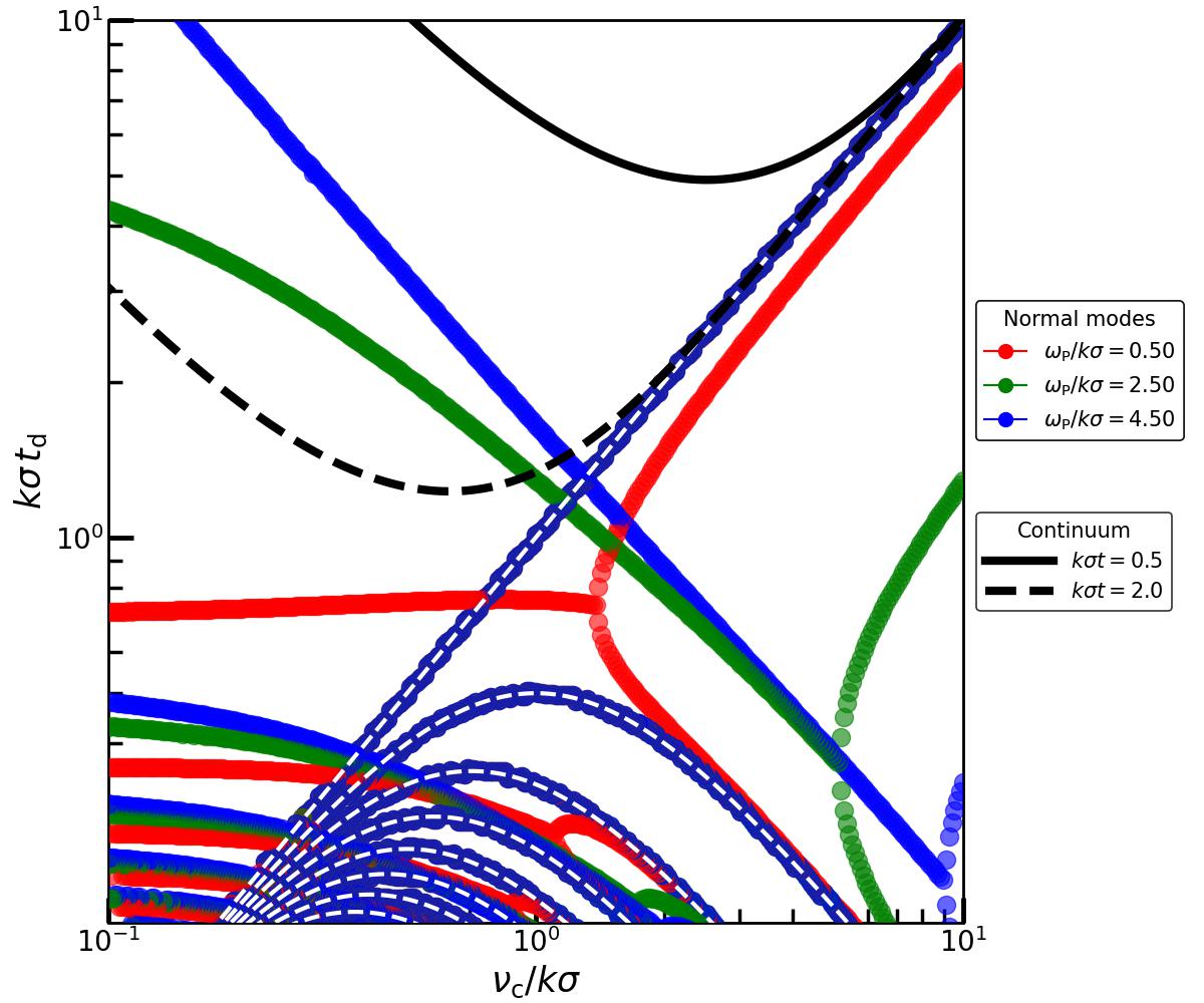
Figure 4: The damping time, $t_{\rm d}$ (in units of $1/k\sigma$), of the normal modes and the continuum as a function of $\nu_{\rm c}/k\sigma$. The red, green and blue dots indicate the normal modes for three different values of $\omega_{\rm P}/k\sigma$ as indicated. The white dashed lines denote the normal modes of the Lenard-Bernstein (LB) branch. The rest belong to the Landau branch. The solid and dashed lines denote the damping time of the continuum response at $t=0.5$ and $2/k\sigma$ respectively. Note that at small time ($t\lesssim 1/\nu_{\rm c}$), the continuum response damps slower than the normal modes. At later times, the normal modes damp slower than the continuum for $\nu_{\rm c}<k\sigma$. For $\nu_{\rm c}>k\sigma$, the continuum response damps at the same rate as the zero-th order LB mode. The normal modes of the Landau branch smoothly tend to the Landau modes in the $\nu_{\rm c}/k\sigma\to 0$ limit. At $\nu_{\rm c}\approx 2\omega_{\rm P}$, the Landau branch modes bifurcate and transition from being oscillatory (for $\nu_{\rm c}\lesssim 2\omega_{\rm P}$) to non-oscillatory (for $\nu_{\rm c}\gtrsim 2\omega_{\rm P}$).

The normal mode spectrum of a weakly collisional plasma has a rich structure. As shown by [20, 10, etc.], all modes in a plasma that is perturbed around an $f_{0}$ with $\partial f_{0}/\partial v<0$ (e.g., the Maxwellian DF) are damped, i.e., have ${\rm Re}(\gamma)<0$. The damping time is given by $t_{\rm d}=1/\left|{\rm Re}(\gamma)\right|$. Fig. 4 plots this damping time (in units of $1/k\sigma$), as a function of $\nu_{\rm c}/k\sigma$. The different colors denote different values of $\omega_{\rm P}/k\sigma$ as indicated. The white dashed lines trace out a particular family of modes called the Lenard-Bernstein or LB modes, which are non-oscillating (discussed in detail in section V.2). The black solid and dashed lines indicate the damping time of the continuum response, defined as ${\left|\partial\ln{g_{1\kappa}^{\rm cont}}/\partial t\right|}^{-1}$, at $t=0.5$ and $2$ times $1/k\sigma$, respectively. Since the continuum response scales as $\sim\exp{\left[-{(k\sigma)}^{2}\nu_{\rm c}t^{3}/3\right]}$ at small time, and the modal response scales as $\sim\exp{\left[-\gamma t\right]}$ throughout, the continuum response dominates over the normal modes at short times. At long times, the normal modes dominate on scales smaller than the mean free path ($k>\nu_{\rm c}/\sigma$). However, on scales larger than the mean free path ($k<\nu_{\rm c}/\sigma$), the dominant modes are the continuum as well as the least damped normal mode, which is one of the non-oscillating LB modes (see section V.2 for details).

The normal modes in a weakly collisional plasma are diverse in nature and deserve a systematic categorization. We identify two distinct classes of normal modes: (i) the Landau branch, which analytically continues to the Landau modes in the collisionless limit ($\nu_{\rm c}\ll k\sigma$), and (ii) the Lenard-Bernstein (LB) branch, which consists of an extra set of modes that appear in addition to the Landau-like modes for non-zero $\nu_{\rm c}$. We now discuss these two families of normal modes in detail.

V.1 Landau branch

The modes belonging to the Landau branch analytically continue to the Landau modes in the collisionless ($\nu_{\rm c}/k\sigma\to 0$) limit. As evident from Fig. 4, the damping timescales of the Landau branch modes tend towards the Landau values in the $\nu_{\rm c}/k\sigma\to 0$ limit, unlike the LB branch modes, indicated by the white dashed lines, whose damping times tend to zero. The analytic continuation to the Landau values can also be seen by rewriting the dispersion relation given in equation (41) in the following form [10]:

$$D(k,\gamma) =1+\frac{\omega^{2}_{\rm P}}{\nu_{\rm c}}\int_{0}^{\infty}{\rm d}s\,\left(1-\exp{\left[-\nu_{\rm c}s\right]}\right)$$

$$\times\exp{\left[-\left(\gamma+\frac{k^{2}\sigma^{2}}{\nu_{\rm c}}\right)s+\frac{k^{2}\sigma^{2}}{\nu_{\rm c}^{2}}\left(1-e^{-\nu_{\rm c}s}\right)\right]}=0.$$ (43)

In the $\nu_{\rm c}/k\sigma\to 0$ limit, this reduces to the Landau dispersion relation [20],

$$D(k,\gamma)=1+\omega^{2}_{\rm P}\int_{0}^{\infty}{\rm d}s\,s\exp{\left[-\left(\gamma s+\frac{k^{2}\sigma^{2}s^{2}}{2}\right)\right]}=0.$$ (44)

The solutions of this equation are the Landau modes, $\gamma_{0}$, which are complex. For each $k$, there are infinitely many discrete modes. Of these, the least damped modes have the following asymptotic form [20]:

$$\gamma_{0} =-2k\sigma\sqrt{\ln{\left({k\sigma}/{\omega_{\rm P}}\right)}}\pm\frac{i\pi}{2}\frac{k\sigma}{\sqrt{\ln{\left({k\sigma}/{\omega_{\rm P}}\right)}}},\qquad\qquad\qquad\qquad\;\,k\sigma\gg\omega_{\rm P},$$

$$=-\sqrt{\frac{\pi}{8}}\,k\sigma\,{\left(\frac{\omega_{\rm P}}{k\sigma}\right)}^{4}\exp{\left[-\frac{1}{2}{\left(\frac{\omega_{\rm P}}{k\sigma}\right)}^{2}\right]}\pm i\omega_{\rm P}\left[1+\frac{3}{2}{\left(\frac{k\sigma}{\omega_{\rm P}}\right)}^{2}\right],\qquad\,k\sigma\ll\omega_{\rm P}.$$ (45)

The above form shows that, in the collisionless limit, the modes are oscillatory and very weakly damped on scales much larger than the Debye scale ($k\ll k_{\rm D}=\omega_{\rm P}/\sigma$). These are also known as Langmuir modes. On scales smaller than the Debye scale ($k\gg k_{\rm D}$), the modes are oscillatory but strongly damped. Hence, oscillations in a collisionless plasma are damped by collective excitations only within the Debye scale.

The Landau modes are modified in presence of collisions, i.e., for non-zero $\nu_{\rm c}$. Let us compute the leading order correction to $\gamma$ in presence of collisions, using linear perturbation theory in the neighborhood of the Landau modes, $\gamma_{0}$ (taking $\nu_{\rm c}\ll\min{\left[\gamma_{0},k\sigma\right]}$). We expand $\gamma$ about $\gamma_{0}$ as $\gamma=\gamma_{0}+\nu_{\rm c}\,\delta_{1}$. Then, we rewrite the dispersion relation given in equation (43) by only retaining terms that are zero-th and linear order in $\nu_{\rm c}$, as follows:

$$D(k,\gamma_{0}+\nu_{\rm c}\delta_{1})$$

$$=1+\omega^{2}_{\rm P}\int_{0}^{\infty}{\rm d}s\,\left[s-\nu_{\rm c}s^{2}\left(\delta_{1}+\frac{1}{2}-\frac{k^{2}\sigma^{2}s^{2}}{6}\right)\right]$$

$$\times\exp{\left[-\left(\gamma_{0}s+\frac{k^{2}\sigma^{2}s^{2}}{2}\right)\right]}=0.$$ (46)

Using that $\gamma_{0}$ follow the Landau dispersion relation (equation [44]), and performing the $s$ integrals, we obtain:

$$\delta_{1}=\frac{\gamma-\gamma_{0}}{\nu_{\rm c}}=-\frac{1}{2}+\frac{1}{6}\frac{P(\gamma_{0}/k\sigma)}{Q(\gamma_{0}/k\sigma)},$$ (47)

where

$$P\left(\frac{\gamma_{0}}{k\sigma}\right)=\left[{\left(\frac{\gamma_{0}}{k\sigma}\right)}^{3}+4\frac{\gamma_{0}}{k\sigma}\right]$$

$$+\,\left[{\left(\frac{\gamma_{0}}{k\sigma}\right)}^{4}+6{\left(\frac{\gamma_{0}}{k\sigma}\right)}^{2}+3\right]\sqrt{\frac{\pi}{2}}\left[1+{\rm erf}\left(\frac{\gamma_{0}}{k\sigma}\right)\right]\exp{\left[\frac{1}{2}{\left(\frac{\gamma_{0}}{k\sigma}\right)}^{2}\right]},$$

$$Q\left(\frac{\gamma_{0}}{k\sigma}\right)=\frac{\gamma_{0}}{k\sigma}$$

$$+\,\left[{\left(\frac{\gamma_{0}}{k\sigma}\right)}^{2}+1\right]\sqrt{\frac{\pi}{2}}\left[1+{\rm erf}\left(\frac{\gamma_{0}}{k\sigma}\right)\right]\exp{\left[\frac{1}{2}{\left(\frac{\gamma_{0}}{k\sigma}\right)}^{2}\right]}.$$ (48)

On scales much larger than the Debye length ($k\sigma\ll\omega_{\rm P}$), $\gamma_{0}/k\sigma\to 0$, and therefore, $P/Q\to 0$. This implies that $\delta_{1}\to-\frac{1}{2}$, and therefore

$$\gamma\approx\gamma_{0}-\frac{\nu_{\rm c}}{2}$$ (49)

on large scales. In Fig. 4, this is evident from the linear decrease with $\nu_{\rm c}$ (at large $\nu_{\rm c}$) of the damping time of the most weakly damped modes for the $\omega_{\rm P}/k\sigma=4.5$ and $2.5$ cases, indicated by the blue and green lines respectively.

Let us now investigate the case of frequent collisions, i.e., when $\nu_{\rm c}\gtrsim k\sigma$. As evident from Fig. 4, the modes remain oscillatory but become more strongly damped with increasing $\nu_{\rm c}$, until a bifurcation occurs and they become non-oscillatory. At bifurcation, the complex frequencies of the modes become purely real and negative. The bifurcation occurs when $\nu_{\rm c}\sim 2\omega_{\rm P}$, i.e., when the mean free path, $\lambda_{\rm c}=\sigma/\nu_{\rm c}$, is roughly half the Debye length, $\lambda_{\rm D}=\sigma/\omega_{\rm P}$. Each bifurcation results in a less damped upper branch and a more damped lower branch. For the zeroth order modes (which analytically continue to the least damped Landau modes in the $\nu_{\rm c}/k\sigma\to 0$ limit), the damping timescale of the upper branch scales as $t_{\rm d}\sim\nu_{\rm c}$ while that of the lower branch scales as $t_{\rm d}\sim 1/\nu_{\rm c}$ in the $\nu_{\rm c}\gg 2\omega_{\rm P}$ limit. Hence, the zero-th order Landau branch mode is very weakly damped, albeit non-oscillatory for $\nu_{\rm c}\gg 2\omega_{\rm P}$. For the higher order modes, the damping timescales of both branches scale as $t_{\rm d}\sim 1/\nu_{\rm c}$, i.e., these modes are strongly damped as well as non-oscillatory in the $\nu_{\rm c}\gg 2\omega_{\rm P}$ limit.

The above behaviour of the modes at large $\nu_{\rm c}/2\omega_{\rm P}$ can be readily seen by analyzing the dispersion relation in the $\nu_{\rm c}/k\sigma\to\infty$ limit. We follow [10] to obtain the following form for the dispersion relation (for the zero-th order mode) in this limit:

$$D(k,\gamma)=1+{\left(\frac{\omega_{\rm P}}{\nu_{\rm c}}\right)}^{2}\int_{0}^{\infty}{\rm d}x\,x^{\gamma/\nu_{\rm c}-1}(1-x)=0,$$ (50)

which can be integrated to yield

$$1+{\left(\frac{\omega_{\rm P}}{\nu_{\rm c}}\right)}^{2}\left[\frac{1}{\gamma/\nu_{\rm c}}-\frac{1}{\gamma/\nu_{\rm c}+1}\right]=0.$$ (51)

This is a quadratic equation in $\gamma/\nu_{\rm c}$ and has the following solutions:

$$\frac{\gamma}{\nu_{\rm c}}=-\frac{1}{2}\left[1\pm\sqrt{1-{\left(\frac{2\omega_{\rm P}}{\nu_{\rm c}}\right)}^{2}}\right].$$ (52)

The frequencies are complex conjugate, i.e., the zero-th order modes are damped but oscillating for $\omega_{\rm P}>\nu_{\rm c}/2$. At $\omega_{\rm P}=\nu_{\rm c}/2$, a bifurcation occurs and the frequencies become negative real, i.e., the modes become non-oscillatory and damped. For $\nu_{\rm c}\gg 2\omega_{\rm P}$, the upper branch mode has $\gamma\approx-\omega^{2}_{\rm P}/\nu_{\rm c}$ and is weakly damped, while the lower branch one has $\gamma\approx-\nu_{\rm c}$ and is strongly damped.

From Fig. 4 as well as the above analysis, we see that the normal modes are more strongly damped than the Landau modes of the collisionless limit when $\nu_{\rm c}<2\omega_{\rm P}$. At $\nu_{\rm c}\approx 2\omega_{\rm P}$, each of these modes bifurcates into two non-oscillatory modes, one of which is less damped than the other. The less damped mode eventually becomes more weakly damped than the corresponding Landau mode at $\nu_{\rm c}\gg 2\omega_{\rm P}$. Therefore, collisions facilitate the collective, Landau-like damping of plasma perturbations for $\nu_{\rm c}<2\omega_{\rm P}$, i.e., when the mean free path, $\lambda_{\rm c}=\sigma/\nu_{\rm c}$, exceeds half the Debye length, $\lambda_{\rm D}=\sigma/\omega_{\rm P}$. On the other hand, for $\nu_{\rm c}\gg 2\omega_{\rm P}$, i.e., $\lambda_{\rm c}\ll\lambda_{\rm D}/2$, collisions oppose Landau damping, but make the modes non-oscillating. Since the mean free path is smaller than the Debye length in this case, collisional scatterings destroy the coherence of the collective oscillations.

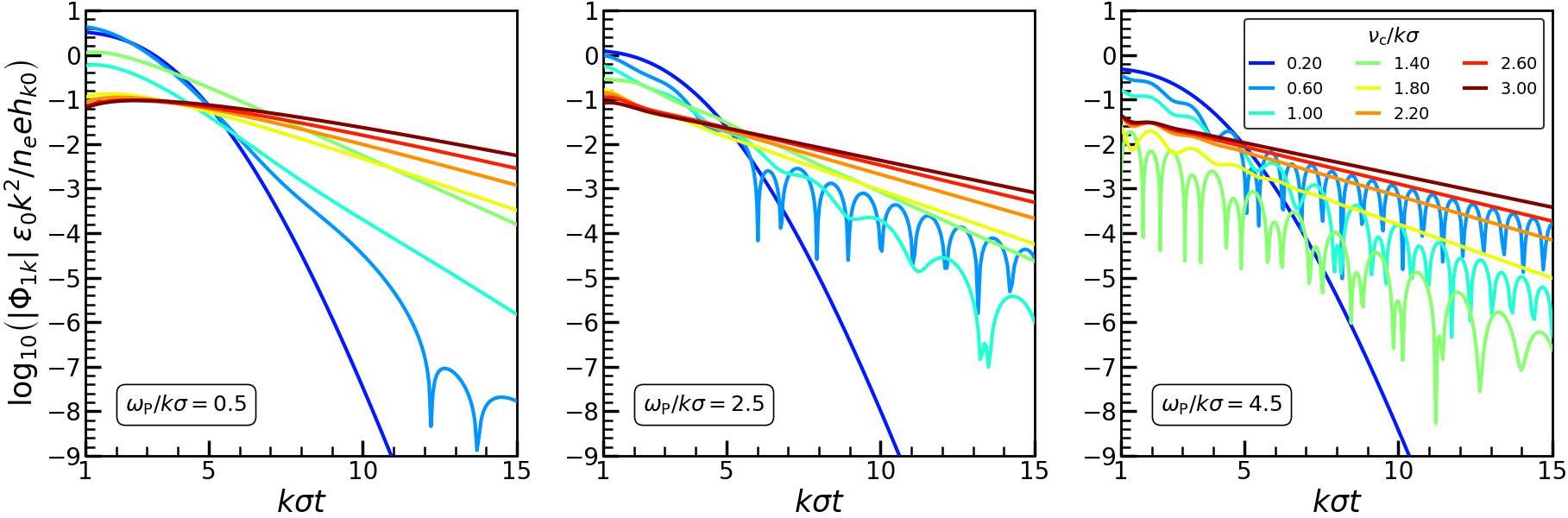
Figure 5: The combined temporal response of a weakly collisional plasma, including both the continuum and the normal modes, in terms of $\left|\Phi_{1k}\right|$ vs $t$ (in units of $1/k\sigma$). The initial perturbation in the DF is taken to be a Dirac delta function in $v$ ($s=\sigma_{0}/\sigma=0$). Different colors indicate the response for different values of $\nu_{\rm c}/k\sigma$, and different panels correspond to different values of $\omega_{\rm P}/k\sigma$ as indicated. The initial phase of the decay, up to $t\sim 1/\nu_{\rm c}$, is driven by the continuum. For $\nu_{\rm c}<k\sigma$, the latter phase of the decay is driven by the normal modes, while for $\nu_{\rm c}>k\sigma$, the long term decay is governed by the continuum and the zero-th order LB mode, which is a non-oscillatory mode.

V.2 Lenard-Bernstein Branch

The collision operator in the Boltzmann equation involves the highest velocity derivative and is therefore a singular perturbation to the collisionless Boltzmann equation. This implies that the normal mode spectrum for the weakly collisional case is qualitatively different from the collisionless case. Therefore, in addition to the Landau branch modes discussed above, the LB operator introduces an additional set of modes, which we term Lenard-Bernstein or LB modes. We indicate these using white dashed lines in Fig. 4. Unlike the Landau branch modes, the LB modes do not analytically continue to the Landau modes in the collisionless limit. Moreover, the LB modes are damped and non-oscillatory. As also found by [10], the frequencies of these modes are given by

$$\frac{\gamma}{\nu_{\rm c}}=-{\left(\frac{k\sigma}{\nu_{\rm c}}\right)}^{2}-n,$$ (53)

where $n=0,1,2,...\,$. These modes are independent of the plasma frequency and therefore completely decoupled from the mean electrostatic field. These solely depend on $\nu_{\rm c}$, and are thus pure manifestations of short range collisional scatterings in the plasma. The $n\neq 0$ modes are heavily damped, especially in large and small $\nu_{\rm c}/k\sigma$ limits, since $\gamma\approx-n\nu_{\rm c}$ for $\nu_{\rm c}\gg k\sigma$ and $\gamma\approx-{\left(k\sigma\right)}^{2}/\nu_{\rm c}$ for $\nu_{\rm c}\ll k\sigma$. On the other hand, the $n=0$ mode is heavily damped for small $\nu_{\rm c}/k\sigma$ but very weakly damped in the large $\nu_{\rm c}/k\sigma$ limit, since $\gamma=-{\left(k\sigma\right)}^{2}/\nu_{\rm c}$ throughout.

The LB modes play a crucial role in plasma relaxation in the large $\nu_{\rm c}/k\sigma$ limit. The damping timescale of the LB modes scales with $\nu_{\rm c}$ in the same way as that of the Landau branch modes in this limit. Also, in this limit, the damping time of the continuum response is the same as that of the $n=0$ LB mode. Hence, it is the LB modes that dictate the relaxation of plasmas in the limit of frequent collisions, or equivalently on scales larger than the mean free path.

VI Combined temporal response

In the above sections, we separately computed the continuum and normal mode parts of the response. The combined response of a plasma is a temporal convolution of the two. This can be readily seen by studying the evolution of the potential perturbation, $\Phi_{1k}(t)$. Note that $\Phi_{1k}=-(2\pi n_{e}e/\epsilon_{0})(G_{1\kappa}(0)/k^{2})$, where $G_{1\kappa}(0)$ is the inverse Laplace transform of $\tilde{G}_{1\kappa}(0)$, given in equation (16). To compute the inverse Laplace transform, we make use of the identity,

$${\cal L}^{-1}\left(\tilde{f}(\gamma)\tilde{g}(\gamma)\right) =\frac{1}{2\pi i}\int_{c-i\infty}^{c+i\infty}{\rm d}\gamma\,\tilde{f}(\gamma)\tilde{g}(\gamma)\exp{\left[\gamma t\right]}$$

$$=\int_{0}^{t}{\rm d}\tau\,f(\tau)\,g(t-\tau),$$ (54)

where $f$ and $g$ are the inverse Laplace transforms of $\tilde{f}$ and $\tilde{g}$ respectively. For our problem, $\tilde{f}$ and $\tilde{g}$ correspond to $N$ and $1/D$ respectively, with $N$ and $D$ given by equations (17).

For an initial Gaussian pulse, $h_{\kappa}(u)$, given by equation (21), we find that, for $t\gtrsim 1/k\sigma$, the potential response is given by

$$\Phi_{1k}(t)=-\frac{n_{e}e}{\epsilon_{0}}\frac{h_{\kappa 0}}{k^{2}}\sum_{n}\frac{\exp{\left[\gamma_{n}t\right]}}{D^{\prime}\left(\kappa,\gamma_{n}\right)}\int_{0}^{k\sigma t}{\rm d}z\,\exp{\left[-\left(\frac{\gamma_{n}}{k\sigma}+\kappa\right)z+\frac{\kappa^{2}}{2}\left(1-e^{-z/\kappa}\right)\left\{\left(1-s^{2}\right)\left(1-e^{-z/\kappa}\right)+2\right\}-i\kappa u_{0}\left(1-e^{-z/\kappa}\right)\right]},$$ (55)

where $\kappa=k\sigma/\nu_{\rm c}$, $s=\sigma_{0}/\sigma$, and $u_{0}=v_{0}/\sigma$ with $v_{0}$ the drift velocity and $\sigma_{0}$ the velocity dispersion of the initial Gaussian (in $v$) pulse. $\gamma_{n}$ are the frequencies of the normal modes that follow the dispersion relation, $D\left(\kappa,\gamma_{n}\right)=0$, given in equation (41). $D^{\prime}$ refers to the derivative of $D$ with respect to $\gamma_{n}/k\sigma$ and is given by

$$D^{\prime}\left(\kappa,\gamma_{n}\right) =-\frac{\omega^{2}_{\rm P}}{k\sigma\nu_{\rm c}}e^{\zeta}\left[\zeta^{-a_{n}}\gamma(a_{n},\zeta)\right.$$

$$\left.-\Gamma^{2}(a_{n})(a_{n}-\zeta)\,{}_{2}F_{2}(a_{n},a_{n};a_{n}+1,a_{n}+1;-\zeta)\right],$$ (56)

where $a_{n}=\gamma_{n}/\nu_{\rm c}+\kappa^{2}$, $\zeta=\kappa^{2}$, and ${}_{2}F_{2}$ refers to the confluent hypergeometric function of the second kind.

Let us investigate the temporal behaviour of $\Phi_{1k}$ in some detail. Fig. 5 plots $\Phi_{1k}$ in units of $n_{e}eh_{\kappa 0}/\epsilon_{0}k^{2}$ as a function of time (in units of $1/k\sigma$) for $s=0$, i.e., an initial Dirac delta pulse in $v$, for eight different values of $\nu_{\rm c}/k\sigma$ as indicated and for three different values of $\omega_{\rm P}/k\sigma$ in three different panels. There are several key features of the response. It decays as $\sim\exp{\left[-{\left(k\sigma\right)}^{2}\nu_{\rm c}t^{3}/3\right]}$ at small time and transitions to an exponential decay at large time. The long time exponential decay rate is given by $\min{\left[{\rm Re}\left(\gamma_{0}\right),{\left(k\sigma\right)}^{2}/\nu_{\rm c}\right]}$, where $\gamma_{0}$ is the frequency of the least damped normal mode. For $\nu_{\rm c}\gtrsim 2\omega_{\rm P}$, i.e., when the mean free path is somewhat smaller than the Debye length, this decay rate is $\sim{\left(k\sigma\right)}^{2}/\nu_{\rm c}$. The transition from the initial super-exponential decay to the late time exponential decay is more pronounced on scales comparable to the mean free path ($\nu_{\rm c}\sim k\sigma$). On scales much smaller than the mean free path ($\nu_{\rm c}\ll k\sigma$), the small time super-exponential decay is governed by the continuum while the long time exponential decay is governed by the least damped normal mode (as evident from the temporal oscillations of the long time response). On scales larger than the mean free path ($\nu_{\rm c}\gg k\sigma$), the response undergoes a slow exponential decay, guided by the weakly damped continuum and the least damped normal mode (the zero-th order non-oscillatory LB mode), over a timescale $\sim\nu_{\rm c}/{\left(k\sigma\right)}^{2}$. For $\omega_{\rm P}\leq\nu_{\rm c}/2$, the response becomes non-oscillatory, as evident from the absence of oscillations in the response for larger values of $\nu_{\rm c}$. All in all, Fig. 5 illustrates the smooth changeover from the super-exponential decay of the response on scales smaller than the mean free path ($\nu_{\rm c}<k\sigma$) and/or in the diffusive regime ($t<1/\nu_{\rm c}$), to the exponential decay on scales larger than the mean free path ($\nu_{\rm c}>k\sigma$) and/or in the friction regime ($t>1/\nu_{\rm c}$).

If the initial DF perturbation is of the Maxwellian form in $v$, the response is given by equation (55), with $s=1$. The response in this case is similar to the Dirac delta case, except that the small time decay now occurs not only due to collisional diffusion but also due to phase-mixing between particles with different velocities. The initial DF perturbation, $f_{1}(0,v)$, has a finite spread in velocities, and the continuum DF response in each $v$ scales as $\sim f_{1}(0,v)\exp{\left[-ikvt\right]}$. When marginalized over $v$, the initial response undergoes phase-mixing and damps away as $\exp{\left[-k^{2}\sigma^{2}t^{2}/2\right]}$. Over long time, however, the response decays exponentially at the rate of $\min{\left[{\rm Re}\left(\gamma_{0}\right),{\left(k\sigma\right)}^{2}/\nu_{\rm c}\right]}$, under the combined action of collective effects (normal modes) and collisional damping, just as in the Dirac delta case.

VII Discussion and summary

We have, for the first time, provided a general formalism for the relaxation of a weakly collisional plasma in the perturbative (linear and second order) regime. Following the seminal work of [10], we compute the response of a weakly collisional plasma using the perturbed Boltzmann-Poisson equations, and demonstrate that the [11] continuum response and the normal modes [10, 7, 8, 9] are nothing but different limits of a general form of the response. Moreover, we show that previous studies had missed out on a crucial limit of the continuum response: at late times and on large scales, the continuum response undergoes a much slower decay than what [11] predicts. This finding has important implications for a number of phenomena such as the collisional damping of the plasma echo, dissipation in astrophysical shocks, etc., and provides a rigorous justification for the establishment of local thermal equilibrium in the fluid limit. This hitherto unknown limit of the continuum response is crucial for drawing a bridge between the collisionless and fluid limits of plasma relaxation.

We describe a weakly collisional plasma using a perturbative analysis of the Boltzmann-Poisson equations. We assume that collisional relaxation is dominated by weak deflections of electrons from their orbits, and therefore model collisions using a collision operator of the Fokker-Planck type, called the Lenard-Bernstein (LB) operator [10], given by equation (7). The collision frequency, $\nu_{\rm c}$, parametrizes the rate of collisions. The collision operator consists of two terms: a diffusion term proportional to $\sigma^{2}\partial^{2}f/\partial v^{2}$ and a damping/friction term proportional to $\partial(vf)/\partial v$. Although one considers both terms to obtain the normal mode spectrum in the standard theory [10], the analysis of the continuum spectrum has so far only been performed using the diffusion term [11, 12]. This approximation simplifies the calculations but is inconsistent with the fluctuation-dissipation theorem. It is only valid in a limited spatio-temporal domain: at times smaller than the collision time and on scales smaller than the mean free path, i.e., only within the boundary layer. We include both the diffusion and friction terms in the collision operator, and obtain the full response, which is a combination of the continuum response and the normal modes. In fact, we find that the total response is a temporal convolution of the two. The continuum dominates the initial part of the response, while the long time response has contribution from both normal modes and the continuum.

Collisions affect the normal modes and the continuum in different ways. The normal mode response exponentially damps away due to a combination of collective Landau damping and collisional effects; the frequencies and damping rates of the normal modes get shifted from the Landau values in presence of collisions. When $\nu_{\rm c}<2\omega_{\rm P}$, collisions enhance the damping rate of the normal modes above the Landau damping rate of collisionless plasma. For $\nu_{\rm c}\gtrsim 2\omega_{\rm P}$, collisions make the modes non-oscillatory and purely damped. For $\nu_{\rm c}\gg 2\omega_{\rm P}$, the damping rates of the modes become weaker than the corresponding Landau damping rates. Therefore, collisions facilitate the collective damping of the response when they are rare, but oppose damping when they are very frequent.

The continuum part of the response evolves differently with time than the normal modes. At times smaller than the collision time, $1/\nu_{\rm c}$, the continuum decays as $\sim\exp{\left[-{\left(t/t_{{\rm d},1}\right)}^{3}\right]}$ over a damping timescale of $t_{{\rm d},1}\sim\nu_{\rm c}^{-1/3}{\left(k\sigma\right)}^{-2/3}$, similar to the prediction by [11]. At $t>1/\nu_{\rm c}$, however, it goes over to an exponential decay over a timescale of $t_{{\rm d},2}\sim\nu_{\rm c}/{\left(k\sigma\right)}^{2}$. The response damps away the most on scales comparable to the mean free path, i.e., for $\nu_{\rm c}\sim k\sigma$. On smaller scales the decay is super-exponential, as predicted by [11], but on scales larger than the mean free path, the decay is exponential and gets slower with increasing $\nu_{\rm c}$. The pronounced damping of the response for $\nu_{\rm c}\sim k\sigma$ is also seen by [21] in their simulations, who note that the collision frequency suitable for preventing the numerical recurrence of initial conditions (echo) is a function of the wavenumber of the perturbation. Our analysis shows that this wavenumber is nothing but $\sim\nu_{\rm c}/\sigma$, the inverse of the mean free path. We supplement the Fokker-Planck analysis of the continuum response with a complementary analysis of stochastic collisional scattering using the Langevin equation, in the same spirit as the study of Brownian motion [15, 16]. We model the effect of collisional diffusion by a stochastic acceleration term corresponding to white noise, and that of collisional damping by a friction term. The resulting velocity dispersion increases linearly with time and then saturates to the equilibrium value, $\sigma^{2}$, after $t\sim 1/\nu_{\rm c}$. Meanwhile, the dispersion in position increases as $\sim t^{3}$ for $t\lesssim 1/\nu_{\rm c}$ and as $\sim t$ for $t\gtrsim 1/\nu_{\rm c}$. This is a classic feature of random walk or diffusion in the velocity space, followed by damping or friction in the velocity space and diffusion in the position space. The cubic exponential decay of the continuum response for $t<1/\nu_{\rm c}$, followed by an exponential decay for $t>1/\nu_{\rm c}$, is a consequence of collisional diffusion followed by damping. We infer that the temporal nature of continuum decay obtained in this paper is not particularly sensitive to the Lenard-Bernstein form of the collision operator, but is a robust phenomenon (at least qualitatively) in any system governed by short range random/chaotic collisions.

The general treatment of plasma relaxation discussed in this paper shows that the [11] scaling of continuum decay is only valid for small time and on scales smaller than the mean free path. This is expected since the [11] calculation neglects the damping term in the LB operator, and entirely relies on a boundary-layer analysis, as also demonstrated by [12]. Therefore, one should be cautious about the limited range of validity of the [11] result when addressing phenomena pertaining to collisional diffusion in plasmas. One such phenomenon is the non-linear effect of plasma echo, a macroscopic disturbance that occurs due to the interference of the (continuum) responses to two subsequent pulses (with wavenumber $k_{1}$ and $k_{2}$) of electric field. We infer that, with increasing $\nu_{\rm c}$, the echo time approaches the time of initiation of the second pulse, and becomes harder, albeit possible, to detect. Contrary to what [11] predict, we infer that the echo is detectable even for $\nu_{\rm c}$ as large as $\sim\left(k_{1}-k_{2}\right)\sigma$, as long as the second pulse is introduced within a few phase-mixing timescales after the first pulse.

The essential features of plasma relaxation described in this paper can be understood by comparing the plasma frequency, $\omega_{\rm P}$, the collision frequency, $\nu_{\rm c}$, and the phase-mixing frequency, $k\sigma$, or alternatively by comparing three different length scales: the Debye length, $\lambda_{\rm D}=\sigma/\omega_{\rm P}$, the mean free path, $\lambda_{\rm c}=\sigma/\nu_{\rm c}$, and the perturbation scale, $\lambda\sim 1/k$. The self-limiting nature of collisions is manifest in the stagnated damping of both the normal modes and the continuum beyond certain scales. The damping of the normal modes occurs efficiently for $\nu_{\rm c}\lesssim 2\omega_{\rm P}$, but gets stagnated for $\nu_{\rm c}\gtrsim 2\omega_{\rm P}$. In other words, collisions facilitate the collective Landau-like damping of the normal modes when the mean free path, $\lambda_{\rm c}=\sigma/\nu_{\rm c}$, is larger than half the Debye length, $\lambda_{\rm D}=\sigma/\omega_{\rm P}$, and oppose collective damping when $\lambda_{\rm c}\lesssim\lambda_{\rm D}/2$. The normal modes, however, become non-oscillating for $\lambda_{\rm c}\lesssim\lambda_{\rm D}/2$, since multiple collisional scatterings within the Debye scale destroy the coherence of the collective plasma oscillations. The collisional damping of the continuum response occurs rapidly for $\nu_{\rm c}\sim k\sigma$ or $\lambda\sim\lambda_{\rm c}$, but is arrested for $\nu_{\rm c}>k\sigma$ or $\lambda>\lambda_{\rm c}$. This transition of the damping rate at $\lambda\sim\lambda_{\rm c}$ owes to the fact that the collisional diffusion of particle velocities is restricted within the mean free path. This means that a local thermal equilibrium (LTE) is established only within the mean free path since the DF approaches the Maxwellian form locally (within $\lambda_{\rm c}$ around a point), after a collision time, $1/\nu_{\rm c}$. As a result, a local equation of state can be adopted and a fluid formalism implemented to study the evolution of plasma perturbations on scales above the mean free path. An ideal fluid description is, however, only valid as long as $\nu_{\rm c}\ll 2\omega_{\rm P}$, or the mean free path, $\lambda_{\rm c}$, is substantially larger than $\lambda_{\rm D}/2$. When $\nu_{\rm c}\gtrsim 2\omega_{\rm P}$, or $\lambda_{\rm c}\lesssim\lambda_{\rm D}/2$, the normal modes are rendered non-oscillatory by collisions. Therefore, an ideal fluid description becomes questionable in this regime. To properly study the long time relaxation of plasmas in this regime, one should either use a collisional kinetic theory formalism as described in this paper, or incorporate viscous dissipation in the corresponding fluid formalism.

The temporal behaviour of plasma response computed in this paper relies on the crucial assumption that collisions are weak, in the sense that they cause small deflections of electrons from their unperturbed orbits, such that the collision operator can be modelled as a Fokker-Planck type operator. Following [10, 7, 8, 9], we have adopted a special form of the Fokker-Planck collision operator, the LB operator, which relies on the assumption that the collisions are not only weak but also sufficiently short range and random/chaotic (so that the collisional dynamics can be modelled as a Markovian random walk). This simplifies the computation of the normal mode spectrum. Despite its simplicity, the LB operator captures the essential physics of weak collisions. We believe that the qualitative features of the perturbative relaxation of a weakly collisional plasma are independent of the exact form of the collision operator. Of course, this needs to be verified using a more realistic collision operator such as the Landau operator or the Balescu-Lenard operator, which we leave for future investigation.

We have developed a general formalism for the perturbative (linear and second order) relaxation of weakly collisional plasmas in this paper. It would be interesting to investigate the effect of weak collisions also on the non-linear relaxation of plasmas. The crucial role of collisional damping or friction in breaking the symmetry of wave-particle resonances (shifting and splitting of resonance lines) during the quasilinear relaxation of plasmas has been noted by [22]. Their analysis is, however, restricted to the domain where the collision frequency significantly exceeds the libration/bounce frequency of charged particles in the trapped region of the phase space. In future work, we intend to investigate quasilinear relaxation when these two frequencies are comparable. In particular, we would like to address the following questions. How does weak collisionality affect the trapping of ions and electrons in the non-linear Bernstein-Green-Kruskal or BGK [23] modes? Is the BGK mode stable in presence of collisions? Do collisions untrap the otherwise trapped particles, and if so, how fast? How do collisions impact the so-called sideband instability [24] of BGK modes? We envision developing a theory for phase space cascade and turbulence in a weakly collisional plasma, similar to that advocated by [25], but including certain key elements that they neglect. We plan to extend the formalism presented in this paper to the study of the impact of weak collisions on self-gravitating systems, since such systems are governed by the Boltzmann-Poisson equations just like plasmas (with the crucial difference that the right-hand-side of the Poisson equation carries the opposite sign relative to the plasma case). This formalism can be applied to the evolution of various astrophysical systems such as globular clusters and self-interacting dark matter halos, where collisions play an important role.

Appendix A Calculation of the linear response

The linear response of a weakly collisional plasma is computed by simultaneously solving the linearized Boltzmann and Poisson equations, which amounts to solving equation (12) for $\tilde{g}_{1\kappa}(u)$. Upon taking the Fourier transform in $u$, this becomes equation (14), which needs to be solved for $\tilde{G}_{1\kappa}(w)$, the Fourier transform of $\tilde{g}_{1\kappa}(u)$. The solution for $\tilde{G}_{1\kappa}(w)$ is given by equation (15), which involves $\tilde{G}_{1\kappa}(0)$. Therefore, substituting $w=0$ in equation (15), we obtain the expression for $\tilde{G}_{1\kappa}(0)$ given in equations (16) and (17). Re-substituting the expression for $\tilde{G}_{1\kappa}(0)$ in equation (15) now yields the following expression for $\tilde{G}_{1\kappa}(w)$:

$$\tilde{G}_{1\kappa}(w) =\tilde{G}^{(1)}_{1\kappa}(w)+\tilde{G}^{(2)}_{1\kappa}(w)+\tilde{G}^{(3)}_{1\kappa}(w),$$ (57)

where

$$\tilde{G}_{1\kappa}^{(1)}(w) =\exp{\left[-\frac{w^{2}}{2}-\kappa w\right]}\;\;{\left(w-\kappa\right)}^{-\left(\eta+\kappa^{2}\right)}\int_{\kappa}^{w}{\rm d}w^{\prime}\,\exp{\left[\frac{w^{\prime 2}}{2}+\kappa w^{\prime}\right]}\;\;{\left(w^{\prime}-\kappa\right)}^{\,\eta+\kappa^{2}-1}H_{\kappa}(w^{\prime}),$$

$$\tilde{G}_{1\kappa}^{(2)}(w) =-\frac{2\pi}{\kappa}{\left(\frac{\omega_{\rm P}}{\nu_{\rm c}}\right)}^{2}\frac{N^{(2)}(\kappa,\eta)}{D(k,\eta)}\times\exp{\left[-\frac{w^{2}}{2}-\kappa w\right]}\;\;{\left(w-\kappa\right)}^{-\left(\eta+\kappa^{2}\right)}\int_{\kappa}^{w}{\rm d}w^{\prime}\,\exp{\left[\frac{w^{\prime 2}}{2}+\kappa w^{\prime}\right]}\;\;{\left(w^{\prime}-\kappa\right)}^{\,\eta+\kappa^{2}-1}w^{\prime}G_{0}(w^{\prime}),$$

$$\tilde{G}_{1\kappa}^{(3)}(w) =-\frac{\kappa A_{\kappa}(\eta)}{D(k,\eta)}\times\exp{\left[-\frac{w^{2}}{2}-\kappa w\right]}\;\;{\left(w-\kappa\right)}^{-\left(\eta+\kappa^{2}\right)}\int_{\kappa}^{w}{\rm d}w^{\prime}\,\exp{\left[\frac{w^{\prime 2}}{2}+\kappa w^{\prime}\right]}\;\;{\left(w^{\prime}-\kappa\right)}^{\,\eta+\kappa^{2}-1}w^{\prime}G_{0}(w^{\prime}).$$ (58)

Here,

$$N^{(2)}(\kappa,\eta) ={\left(-k\right)}^{-\left(\eta+\kappa^{2}\right)}$$

$$\times\int_{\kappa}^{0}{\rm d}w^{\prime}\,\exp{\left[\frac{w^{\prime 2}}{2}+\kappa w^{\prime}\right]}\;\;{\left(w^{\prime}-\kappa\right)}^{\,\eta+\kappa^{2}-1}H_{\kappa}(w^{\prime}),$$ (59)

and

$$D(\kappa,\eta) =1+\frac{2\pi}{\kappa}{\left(\frac{\omega_{\rm P}}{\nu_{\rm c}}\right)}^{2}{\left(-\kappa\right)}^{-\left(\eta+\kappa^{2}\right)}$$

$$\times\int_{\kappa}^{0}{\rm d}w^{\prime}\,\exp{\left[\frac{w^{\prime 2}}{2}+\kappa w^{\prime}\right]}\;\;{\left(w^{\prime}-\kappa\right)}^{\,\eta+\kappa^{2}-1}w^{\prime}G_{0}(w^{\prime})$$

$$=1+{\left(\frac{\omega_{\rm P}}{\kappa\nu_{\rm c}}\right)}^{2}\left[\,1-\left(a-\zeta\right)\zeta^{-a}\exp{\left[\zeta\right]}\,\gamma\left(a,\zeta\right)\,\right],$$ (60)

where $a=\eta+\kappa^{2}$, $\zeta=\kappa^{2}$, and $\gamma(a,\zeta)=\int_{0}^{\zeta}{\rm d}z\,z^{a-1}\exp{\left[-z\right]}$ is the lower incomplete gamma function. We have assumed that the unperturbed DF, $g_{0}$, is of Maxwellian form, i.e., $g_{0}(u)=\exp{\left[-u^{2}/2\right]}\Big{/}\sqrt{2\pi}$, whose velocity Fourier transform is given by

$$G_{0}(w)=\frac{1}{2\pi}\int_{-\infty}^{\infty}{\rm d}u\,\exp{\left[-iwu\right]}\,g_{0}(u)=\frac{1}{2\pi}\exp{\left[-w^{2}/2\right]}.$$ (61)

The temporal response can be computed by taking the inverse Laplace transform and inverse Fourier transform of $\tilde{G}_{1\kappa}(w)$. The three different terms in the expression for $\tilde{G}_{1\kappa}(w)$ given in equation (57) then respectively correspond to three different parts of the response: $\tilde{G}_{1\kappa}^{(1)}$ corresponds to the continuum response, $\tilde{G}_{1\kappa}^{(2)}$ corresponds to the normal modes temporally convoluted with the continuum, and $\tilde{G}_{1\kappa}^{(3)}$ corresponds to the direct response to the perturber or ‘wake’, temporally convoluted with the continuum and the normal modes.

Computation of the continuum part of the response amounts to taking the inverse Laplace transform and inverse Fourier transform (in $u$) of $\tilde{G}_{1\kappa}^{(1)}$ in equation (58). The inverse Laplace transform of ${\left(w-k\right)}^{-\left(\eta+\kappa^{2}\right)}{\left(w^{\prime}-k\right)}^{\left(\eta+\kappa^{2}-1\right)}$ (recall that $\gamma=\nu_{\rm c}\eta$) yields

$${\cal L}^{-1}\left[{\left(w-\kappa\right)}^{-\left(\eta+\kappa^{2}\right)}{\left(w^{\prime}-\kappa\right)}^{\left(\eta+\kappa^{2}-1\right)}\right]$$

$$=\frac{1}{2\pi i}\int_{c-i\infty}^{c+i\infty}{\rm d}\eta\,{\left(w-\kappa\right)}^{-\left(\eta+\kappa^{2}\right)}{\left(w^{\prime}-\kappa\right)}^{\left(\eta+\kappa^{2}-1\right)}\exp{\left[\eta\nu_{\rm c}t\right]}$$

$$=\exp{\left[-\kappa^{2}\nu_{\rm c}t\right]}\;\delta\left[w^{\prime}-\left(we^{-\nu_{\rm c}t}+\kappa\left(1-e^{-\nu_{\rm c}t}\right)\right)\right].$$ (62)

Next, we integrate the inverse Laplace transform of $\tilde{G}_{1\kappa}^{(1)}$ over $w^{\prime}$ and take the inverse Fourier transform in $u$ of the result to obtain the following expression for the continuum response:

$$g_{1\kappa}^{\rm cont}(u,t) =\int_{-\infty}^{\infty}{\rm d}w\,\exp{\left[iwu\right]}\frac{1}{2\pi i}\int_{c-i\infty}^{c+i\infty}{\rm d}\eta\,\exp{\left[\eta\nu_{\rm c}t\right]}\,\tilde{G}_{1\kappa}^{(1)}(w,\eta)$$ (63)

$$=\exp{\left[-\kappa^{2}\nu_{\rm c}t\right]}\int_{-\infty}^{\infty}{\rm d}w\,\exp{\left[iwu\right]}\exp{\left[-\frac{w^{2}}{2}-\kappa w\right]}\int_{\kappa}^{w}{\rm d}w^{\prime}\exp{\left[\frac{w^{\prime 2}}{2}+\kappa w^{\prime}\right]}\delta\left[w^{\prime}-\left(we^{-\nu_{\rm c}t}+\kappa\left(1-e^{-\nu_{\rm c}t}\right)\right)\right]\,H_{\kappa}(w^{\prime})$$

$$=\sqrt{\frac{2}{1-e^{-2\nu_{\rm c}t}}}\exp{\left[-\frac{u^{2}}{2\left(1-e^{-2\nu_{\rm c}t}\right)}\right]}\exp{\left[-\kappa^{2}\left(\nu_{\rm c}t-2\tanh{\frac{\nu_{\rm c}t}{2}}\right)\right]}\exp{\left[-i\kappa u\,\tanh{\frac{\nu_{\rm c}t}{2}}\right]}\,{\cal F}(\kappa,\nu_{\rm c}t),$$ (64)

where

$${\cal F}(w,\kappa,\nu_{\rm c}t)$$

$$=\int_{-\infty}^{\infty}{\rm d}z\,\exp{\left[-{\left\{z+\left(\sqrt{2\tanh{\frac{\nu_{\rm c}t}{2}}}\kappa-i\frac{u}{\sqrt{2\left(1-e^{-2\nu_{\rm c}t}\right)}}\right)\right\}}^{2}\right]}$$

$$\times H_{\kappa}\left(\kappa+ze^{-\nu_{\rm c}t}\right).$$ (65)

In going from the second to third line of equation (64), we have made the substitution, $z=w-\kappa$. The continuum response is evaluated in section IV.1 for different models of $h_{k}(u)$, whose velocity Fourier transform is $H_{k}(w)$.

Appendix B Calculation of velocity and position dispersions in the Langevin formalism

In section IV.2, we gain physical insight into the workings of collisional damping and diffusion by studying the evolution of the first and second moments of the continuum DF response, rather than that of the continuum response itself, which we study in section IV.1. To achieve this, we solve the stochastic Langevin equation, given in equation (31), assuming a collisional friction proportional to $-v$ and a white noise power spectrum for the stochastic acceleration due to collisions. Here we solve this equation to derive the velocity dispersion, $\sigma^{2}(t)$, and the position dispersion, $\sigma^{2}_{x}(t)$.

The Langevin equation (31) can be integrated once with respect to time to yield the following expression for the velocity of a particle:

$$v(t)=\frac{{\rm d}x}{{\rm d}t}=v_{0}\,e^{-\nu_{\rm c}t}+\int_{0}^{t}{\rm d}t^{\prime}\,e^{-\nu_{\rm c}(t-t^{\prime})}\xi(t^{\prime}).$$ (66)

The velocity dispersion, $\sigma(t)$, can now be computed as follows:

$$\sigma^{2}(t) =\left<\left(v(t)-v_{0}\,e^{-\nu_{\rm c}t}\right)^{2}\right>$$

$$=\int_{0}^{t}{\rm d}t^{\prime}\,e^{-\nu_{\rm c}(t-t^{\prime})}\int_{0}^{t}{\rm d}t^{\prime\prime}\,e^{-\nu_{\rm c}(t-t^{\prime\prime})}\left<\xi(t^{\prime})\,\xi(t^{\prime\prime})\right>$$

$$={\cal D}\int_{0}^{t}{\rm d}t^{\prime}\,e^{-\nu_{\rm c}(t-t^{\prime})}\int_{0}^{t}{\rm d}t^{\prime\prime}\,e^{-\nu_{\rm c}(t-t^{\prime\prime})}\delta\left(t^{\prime}-t^{\prime\prime}\right)$$

$$={\cal D}\int_{0}^{t}{\rm d}t^{\prime}e^{-2\nu_{\rm c}t^{\prime}}$$

$$=\sigma^{2}\left(1-e^{-2\nu_{\rm c}t}\right).$$ (67)

In going from the second to the third line, we have used the assumption of a white noise power spectrum for $\xi(t)$, i.e., $\left<\xi(t)\xi(t^{\prime})\right>={\cal D}\delta(t-t^{\prime})$, and in going from the fourth to the fifth line, we have used the Einstein relation that ${\cal D}=\nu_{\rm c}\sigma^{2}$.

Equation (66) can be integrated one more time with respect to time to yield the position of a particle:

$$x(t) =\frac{v_{0}}{\nu_{\rm c}}\left(1-e^{-\nu_{\rm c}t}\right)+\int_{0}^{t}{\rm d}t^{\prime}\int_{0}^{t^{\prime}}{\rm d}t^{\prime\prime}\,e^{-\nu_{\rm c}\left(t^{\prime}-t^{\prime\prime}\right)}\xi(t^{\prime\prime}).$$ (68)

The dispersion in the position, $\sigma_{x}(t)$, is computed as follows:

$$\sigma^{2}_{x}(t) =\left<{\left[x(t)-\frac{v_{0}}{\nu_{\rm c}}\left(1-e^{-\nu_{\rm c}t}\right)\right]}^{2}\right>$$

$$=\int_{0}^{t}{\rm d}t_{1}\int_{0}^{t_{1}}{\rm d}t_{2}\,e^{-\nu_{\rm c}\left(t_{1}-t_{2}\right)}\int_{0}^{t}{\rm d}t_{3}\int_{0}^{t_{3}}{\rm d}t_{4}\,e^{-\nu_{\rm c}\left(t_{3}-t_{4}\right)}\left<\xi(t_{2})\xi(t_{4})\right>$$

$$={\cal D}\int_{0}^{t}{\rm d}t_{1}\int_{0}^{t_{1}}{\rm d}t_{2}\,e^{-\nu_{\rm c}\left(t_{1}-t_{2}\right)}\int_{0}^{t}{\rm d}t_{3}\int_{0}^{t_{3}}{\rm d}t_{4}\,e^{-\nu_{\rm c}\left(t_{3}-t_{4}\right)}\,\delta\left(t_{4}-t_{2}\right),$$ (69)

where, in going from the second to the third line, we have used the assumption that $\left<\xi(t)\xi(t^{\prime})\right>={\cal D}\delta(t-t^{\prime})$. Noting that the integral over $t_{4}$ is non-zero only when $t_{2}\leq t_{3}$, and using the Einstein relation, ${\cal D}=\nu_{\rm c}\sigma^{2}$, we perform the integral over $t_{4}$ to obtain

$$\sigma^{2}_{x}(t) =\nu_{\rm c}\sigma^{2}\int_{0}^{t}{\rm d}t_{1}\,e^{-\nu_{\rm c}t_{1}}\int_{0}^{t_{1}}{\rm d}t_{2}\,e^{2\nu_{\rm c}t_{2}}\int_{t_{2}}^{t}{\rm d}t_{3}\,e^{-\nu_{\rm c}t_{3}}.$$ (70)

Performing the integral over $t_{3}$ yields

$$\sigma^{2}_{x}(t) =\sigma^{2}\int_{0}^{t}{\rm d}t_{1}\,e^{-\nu_{\rm c}t_{1}}\int_{0}^{t_{1}}{\rm d}t_{2}\,\left(e^{\nu_{\rm c}t_{2}}-e^{\nu_{\rm c}\left(2t_{2}-t\right)}\right),$$ (71)

and performing the $t_{2}$ integral yields

$$\sigma^{2}_{x}(t)=\frac{\sigma^{2}}{\nu_{\rm c}}\int_{0}^{t}{\rm d}t_{1}\,\left[1-\frac{3}{2}e^{-\nu_{\rm c}t_{1}}+\frac{1}{2}e^{-\nu_{\rm c}\left(t+t_{1}\right)}\right].$$ (72)

Finally, performing the above $t_{1}$ integral yields the following expression for $\sigma^{2}_{x}(t)$:

$$\sigma^{2}_{x}(t) ={\left(\frac{\sigma}{\nu_{\rm c}}\right)}^{2}\left[\nu_{\rm c}t-\frac{\left(1-e^{-\nu_{\rm c}t}\right)\left(3-e^{-\nu_{\rm c}t}\right)}{2}\right].$$ (73)

Appendix C Calculation of the second order response and the plasma echo

The linear response of a plasma consists of a free streaming continuum and damped normal modes. When marginalized over the velocities, the continuum response phase-mixes away. The non-linear response is, however, fundamentally different in that the continuum response manifests a bunching of particles in the phase space at specific times, leading to macroscopic disturbances in the density. This phenomenon is known as the plasma echo, and can be readily seen at second order in perturbation.

The evolution of the second order response, $f_{2}$, is governed by the following equation:

$$\frac{\partial f_{2}}{\partial t}+v\frac{\partial f_{2}}{\partial x}=-\frac{e}{m}\frac{\partial f_{1}}{\partial v}\frac{\partial\Phi_{\rm P}}{\partial x}+\nu_{\rm c}\frac{\partial}{\partial v}\left(vf_{2}+\sigma^{2}\frac{\partial f_{2}}{\partial v}\right).$$ (74)

Since the echo phenomenon is caused by the continuum response, we ignore the self-potential $\Phi_{1}$ of the plasma that leads to normal modes. Non-dimensionalizing the above equation, then taking the Fourier transform in $x$ and $u=v/\sigma$ and the Laplace transform in $t$ as detailed in section III, we obtain the following differential equation for $\tilde{G}_{2k}(w)$, the Fourier-Laplace mode of $f_{2}$:

$$(w-\kappa)\,\frac{\partial\tilde{G}_{2\kappa}}{\partial w}+(w^{2}+\eta)\,\tilde{G}_{2\kappa}(w,\eta)$$

$$=-w\int{\rm d}\kappa^{\prime}\,\left(\kappa-\kappa^{\prime}\right)\int{\rm d}\eta^{\prime}A_{\kappa-\kappa^{\prime}}(\eta-\eta^{\prime})\,\tilde{G}_{1\kappa^{\prime}}(w,\eta^{\prime}).$$ (75)

Here, we have assumed that $f_{2}(t=0)=0$. The above differential equation can be integrated using the method of integrating factor to yield the following solution for $\tilde{G}_{2\kappa}$:

$$\tilde{G}_{2\kappa}(w,\eta) =-\exp{\left[-\frac{w^{2}}{2}-\kappa w\right]}\;\;{\left(w-\kappa\right)}^{-\left(\eta+\kappa^{2}\right)}\int_{\kappa}^{w}{\rm d}w^{\prime}\,\exp{\left[\frac{w^{\prime 2}}{2}+\kappa w^{\prime}\right]}\;\;{\left(w^{\prime}-\kappa\right)}^{\,\eta+\kappa^{2}-1}w^{\prime}$$

$$\times\int{\rm d}\kappa^{\prime}\,\left(\kappa-\kappa^{\prime}\right)\int{\rm d}\eta^{\prime}A_{\kappa-\kappa^{\prime}}(\eta-\eta^{\prime})\,\tilde{G}_{1\kappa^{\prime}}(w^{\prime},\eta^{\prime}).$$ (76)

The solution for $\tilde{G}_{1\kappa}$ is given by

$$\tilde{G}_{1\kappa}(w,\eta) =-\kappa A_{\kappa}(\eta)\,\exp{\left[-\frac{w^{2}}{2}-\kappa w\right]}\;\;{\left(w-\kappa\right)}^{-\left(\eta+\kappa^{2}\right)}\int_{\kappa}^{w}{\rm d}w^{\prime}\,\exp{\left[\frac{w^{\prime 2}}{2}+\kappa w^{\prime}\right]}\;\;{\left(w^{\prime}-\kappa\right)}^{\,\eta+\kappa^{2}-1}w^{\prime}G_{0}(w^{\prime}),$$ (77)

where we have assumed that $H_{\kappa}(w)=0$, i.e., $f_{1}(t=0)=0$.

For simplicity, we assume hereon that the perturbing potential is impulsive in time. Let the perturbing potential be a combination of two impulses, one at $t=0$ and the other at $t=T$. This implies that

$$\Phi_{k}(t)=t_{\rm P}\left[N_{k}^{(1)}\delta(t)+N_{k}^{(2)}\delta(t-T)\right].$$ (78)

Here, $N_{k}^{(1)}$ and $N_{k}^{(2)}$ are the spatial Fourier transforms of the first and second pulses respectively, and $t_{\rm P}$ is the temporal width of each pulse, which tends towards zero, keeping $N_{k}^{(1)}t_{\rm P}$ and $N_{k}^{(2)}t_{\rm P}$ finite. The Laplace transform of this, for $t>T$, is given by

$$\tilde{\Phi}_{k}(\gamma)=t_{\rm P}\left[N_{k}^{(1)}+N_{k}^{(2)}e^{-\gamma T}\Theta(t-T)\right].$$ (79)

In non-dimensional form, we have

$$A_{\kappa}(\eta)=\frac{\nu_{\rm c}e}{m\sigma^{2}}\tilde{\Phi}_{k}(\gamma)=\nu_{\rm c}t_{\rm P}\left[{\cal A}_{\kappa}+{\cal B}_{\kappa}e^{-\eta\nu_{\rm c}T}\Theta(t-T)\right],$$ (80)

where ${\cal A}_{\kappa}=(e/m\sigma^{2})N_{k}^{(1)}$ and ${\cal B}_{\kappa}=(e/m\sigma^{2})N_{k}^{(2)}$.

Let us first evaluate the linear response, $G_{1\kappa}(w,t)$, which is an essential ingredient of the second order response. Using the result for inverse Laplace transform from equation (62), we get that

$$G_{1\kappa}(w,t) =-\kappa\nu_{\rm c}t_{\rm P}\exp{\left[-\frac{w^{2}}{2}\right]}$$

$$\times\left[{\cal A}_{\kappa}{\cal L}_{\kappa}(w,t)+{\cal B}_{\kappa}{\cal L}_{\kappa}(w,t-T)\,\Theta(t-T)\right],$$ (81)

where

$${\cal L}_{\kappa}(w,t) =\left(we^{-\nu_{\rm c}t}+\kappa\left(1-e^{-\nu_{\rm c}t}\right)\right)$$

$$\times\exp{\left[-\kappa\left(w-\kappa\right)\left(1-e^{-\nu_{\rm c}t}\right)-\kappa^{2}\nu_{\rm c}t\right]}.$$ (82)

Now, let us evaluate the second order response. We inverse Laplace transform equation (76) to obtain

$$G_{2\kappa}(w,t) =-\nu_{\rm c}t_{\rm P}\exp{\left[-\frac{w^{2}}{2}-\kappa w\right]}\int_{\kappa}^{w}{\rm d}w^{\prime}\,\exp{\left[\frac{w^{\prime 2}}{2}+\kappa w^{\prime}\right]}\,w^{\prime}\int{\rm d}\kappa^{\prime}\left(\kappa-\kappa^{\prime}\right)$$

$$\times\left[{\cal A}_{\kappa-\kappa^{\prime}}\exp{\left[-\kappa^{2}\nu_{\rm c}t\right]}\,\delta\left[w^{\prime}-\left(we^{-\nu_{\rm c}t}+\kappa\left(1-e^{-\nu_{\rm c}t}\right)\right)\right]G_{1\kappa^{\prime}}(w^{\prime},0)\right.$$

$$+\left.\Theta\left(t-T\right){\cal B}_{\kappa-\kappa^{\prime}}\exp{\left[-\kappa^{2}\nu_{\rm c}\left(t-T\right)\right]}\,\delta\left[w^{\prime}-\left(we^{-\nu_{\rm c}\left(t-T\right)}+\kappa\left(1-e^{-\nu_{\rm c}\left(t-T\right)}\right)\right)\right]G_{1\kappa^{\prime}}(w^{\prime},T)\right].$$ (83)

Performing the $w^{\prime}$ integral and the velocity Fourier transform of the above, we obtain the second order response as follows:

$$g_{2\kappa}(u,t) =\frac{1}{\sqrt{2\pi}}\exp{\left[-\frac{u^{2}}{2}\right]}\,{\left(\nu_{\rm c}t_{\rm P}\right)}^{2}\int{\rm d}\kappa^{\prime}\kappa^{\prime}\left(\kappa-\kappa^{\prime}\right)\Bigg{[}\,{\cal A}_{\kappa-\kappa^{\prime}}{\cal A}_{\kappa^{\prime}}{\cal I}_{\kappa}(t)+\Theta\left(t-T\right){\cal B}_{\kappa-\kappa^{\prime}}\Big{(}{\cal B}_{\kappa^{\prime}}{\cal I}_{\kappa}(t-T)+{\cal A}_{\kappa^{\prime}}{\cal J}_{\kappa,\kappa^{\prime}}(t,T)\Big{)}\,\Bigg{]},$$ (84)

where

$${\cal I}_{\kappa}(t)=\left[e^{-2\nu_{\rm c}t}+{\left(iue^{-\nu_{\rm c}t}+\kappa\,{\left(1-e^{-\nu_{\rm c}t}\right)}^{2}\right)}^{2}\right]\exp{\left[-\kappa^{2}\left(\nu_{\rm c}t-\frac{\left(1-e^{-\nu_{\rm c}t}\right)\left(3-e^{-\nu_{\rm c}t}\right)}{2}\right)\right]}\exp{\left[-i\kappa u\left(1-e^{-\nu_{\rm c}t}\right)\right]},$$

$${\cal J}_{\kappa,\kappa^{\prime}}(t,T)$$

$$=\left[e^{-\nu_{\rm c}\left(2t-T\right)}\right.$$

$$\left.+\left[iue^{-\nu_{\rm c}\left(t-T\right)}+\kappa{\left(1-e^{-\nu_{\rm c}\left(t-T\right)}\right)}^{2}-\kappa^{\prime}e^{-2\nu_{\rm c}\left(t-T\right)}\left(1-e^{-\nu_{\rm c}T}\right)\right]\left[iue^{-\nu_{\rm c}t}+\kappa e^{-\nu_{\rm c}T}{\left(1-e^{-\nu_{\rm c}\left(t-T\right)}\right)}^{2}+\kappa^{\prime}\left(1-e^{-\nu_{\rm c}T}\right)\left(1-e^{-\nu_{\rm c}\left(2t-T\right)}\right)\right]\right]$$

$$\times\exp{\left[-\kappa^{2}\left(\nu_{\rm c}\left(t-T\right)-\frac{\left(1-e^{-\nu_{\rm c}\left(t-T\right)}\right)\left(3-e^{-\nu_{\rm c}\left(t-T\right)}\right)}{2}\right)\right]}\exp{\left[-{\kappa^{\prime}}^{2}\left(\nu_{\rm c}T-\frac{\left(1-e^{-\nu_{\rm c}T}\right)\left(2+e^{-2\nu_{\rm c}\left(t-T\right)}\left(1-e^{-\nu_{\rm c}T}\right)\right)}{2}\right)\right]}$$

$$\times\exp{\left[-\kappa\kappa^{\prime}\left(1-e^{-\nu_{\rm c}T}\right){\left(1-e^{-\nu_{\rm c}\left(t-T\right)}\right)}^{2}\right]}$$

$$\times\exp{\left[-iu\left(\kappa\left(1-e^{-\nu_{\rm c}\left(t-T\right)}\right)+\kappa^{\prime}e^{-\nu_{\rm c}\left(t-T\right)}\left(1-e^{-\nu_{\rm c}T}\right)\right)\right]}.$$ (85)

Note that ${\cal I}_{\kappa}(t)={\cal J}_{\kappa,\kappa^{\prime}=0}(t,T=0)$.

The above response is a convolution over $k$, and can be simplified if we adopt a perturber potential that is sinusoidal in $x$. Assuming that $\Phi_{\rm P}\sim\exp{\left[ik_{1}x\right]}$ at $t=0$ and $\Phi_{\rm P}\sim\exp{\left[-ik_{2}x\right]}$ at time $T$, we have that ${\cal A}_{\kappa}=a\,\delta(k-k_{1})$ and ${\cal B}_{\kappa}=b\,\delta(k+k_{2})$. Substituting these in equation (84) and performing the integration over $\kappa^{\prime}$ yields the following form for the second order response:

$$g_{2\kappa}(u,t)=\frac{1}{\sqrt{2\pi}}\exp{\left[-\frac{u^{2}}{2}\right]}$$

$$\times\Bigg{[}a^{2}{\left(k_{1}\sigma t_{\rm P}\right)}^{2}\delta\left(k-2k_{1}\right){\cal I}_{\kappa}(t)$$

$$+b^{2}{\left(k_{2}\sigma t_{\rm P}\right)}^{2}\delta\left(k+2k_{2}\right)\Theta(t-T)\,{\cal I}_{\kappa}(t-T)$$

$$-ab\left(k_{1}\sigma t_{\rm P}\right)\left(k_{2}\sigma t_{\rm P}\right)\delta\left(k-\left(k_{1}-k_{2}\right)\right)\Theta(t-T)\,{\cal J}_{\kappa,-\kappa_{2}}(t,T)\Bigg{]}.$$ (86)

The first and second terms denote parts of the response with wavenumbers $2k_{1}$ and $-2k_{2}$ respectively. The third term is a cross-term between the $k_{1}$ and $k_{2}$ modes and manifests an echo of wavenumber $k_{1}-k_{2}$ that occurs slightly after $t=T$. The phase factor in this cross-term becomes independent of $v$, or in other words, phase space bunching occurs at

$$t=t_{\rm echo}\approx T+\frac{1}{\nu_{\rm c}}\ln\left|1+\frac{k_{2}}{k_{1}-k_{2}}\left(1-e^{-\nu_{\rm c}T}\right)\right|.$$ (87)

In the collisionless ($\kappa=k\sigma/\nu_{\rm c}\to\infty$, $\kappa_{2}=k_{2}\sigma/\nu_{\rm c}\to\infty$) limit, the phase factor scales as $\sim\exp{\left[-iv\left(\left(k_{1}-k_{2}\right)t-k_{1}T\right)\right]}$. Accordingly, the $\nu_{\rm c}T\to 0$ limit of equation 87 implies $t_{\rm echo}\approx\left[1+k_{2}/\left(k_{1}-k_{2}\right)\right]T=k_{1}T/\left(k_{1}-k_{2}\right)$. In the strong collision or $\nu_{\rm c}T\to\infty$ limit, $t_{\rm echo}-T\approx\frac{1}{\nu_{\rm c}}\ln{\left|k_{1}/\left(k_{1}-k_{2}\right)\right|}$. Hence, it becomes increasingly difficult to observe the echo with increasing $\nu_{\rm c}$.

The echo is a manifestation of the bunching of particles in the phase space. This implies that the macroscopic density perturbation of the $\left(k_{1}-k_{2}\right)$ mode (obtained by integrating the cross term in $g_{2\kappa}$ from equation [86] over $u$), given by

$$r_{2\kappa}=\frac{\rho_{2k}}{\rho_{0}} =-ab\left(k_{1}\sigma t_{\rm P}\right)\left(k_{2}\sigma t_{\rm P}\right)\delta\left(k-\left(k_{1}-k_{2}\right)\right)\Theta(t-T)$$

$$\times\kappa\left(1-e^{-\nu_{\rm c}(t-T)}\right)\left[\kappa e^{-\nu_{\rm c}T}\left(1-e^{-\nu_{\rm c}(t-T)}\right)-\kappa_{2}\left(1-e^{-\nu_{\rm c}T}\right)\right]$$

$$\times\exp{\left[-\kappa^{2}\left[\nu_{\rm c}\left(t-T\right)-\left(1-e^{-\nu_{\rm c}\left(t-T\right)}\right)\right]-\kappa^{2}_{2}\left[\nu_{\rm c}T-\left(1-e^{-\nu_{\rm c}T}\right)\right]+\kappa\kappa_{2}\left(1-e^{-\nu_{\rm c}\left(t-T\right)}\right)\left(1-e^{-\nu_{\rm c}T}\right)\right]}$$ (88)

peaks around $t=t_{\rm echo}$ (see Fig. 3).

References

- Bruno and Carbone [2005] R. Bruno and V. Carbone, The Solar Wind as a Turbulence Laboratory, Living Reviews in Solar Physics 2, 4 (2005).
- Marsch [2006] E. Marsch, Kinetic Physics of the Solar Corona and Solar Wind, Living Reviews in Solar Physics 3, 1 (2006).
- Howes [2017] G. G. Howes, A prospectus on kinetic heliophysics, Physics of Plasmas 24, 055907 (2017), arXiv:1705.07840 [physics.plasm-ph] .
- Burch et al. [2016] J. L. Burch, T. E. Moore, R. B. Torbert, and B. L. Giles, Magnetospheric Multiscale Overview and Science Objectives, Space Science Reviews 199, 5 (2016).
- Hutchinson [2017] I. H. Hutchinson, Electron holes in phase space: What they are and why they matter, Physics of Plasmas 24, 055601 (2017).
- Chael et al. [2018] A. Chael, M. Rowan, R. Narayan, M. Johnson, and L. Sironi, The role of electron heating physics in images and variability of the Galactic Centre black hole Sagittarius A*, MNRAS 478, 5209 (2018), arXiv:1804.06416 [astro-ph.HE] .
- Ng et al. [1999] C. S. Ng, A. Bhattacharjee, and F. Skiff, Kinetic Eigenmodes and Discrete Spectrum of Langmuir Oscillations in a Weakly Collisional Plasma, in APS Division of Plasma Physics Meeting Abstracts, APS Meeting Abstracts, Vol. 41 (1999) p. CP1.36.
- Ng et al. [2004] C. S. Ng, A. Bhattacharjee, and F. Skiff, Complete Spectrum of Kinetic Eigenmodes for Plasma Oscillations in a Weakly Collisional Plasma, Phys. Rev. Lett. 92, 065002 (2004).
- Ng and Bhattacharjee [2021] C. S. Ng and A. Bhattacharjee, Landau Modes are Eigenmodes of Stellar Systems in the Limit of Zero Collisions, Astrophys. J. 923, 271 (2021), arXiv:2109.07806 [astro-ph.GA] .
- Lenard and Bernstein [1958] A. Lenard and I. B. Bernstein, Plasma Oscillations with Diffusion in Velocity Space, Physical Review 112, 1456 (1958).
- Su and Oberman [1968] C. H. Su and C. Oberman, Collisional Damping of a Plasma Echo, Phys. Rev. Lett. 20, 427 (1968).
- Short and Simon [2002] R. W. Short and A. Simon, Damping of perturbations in weakly collisional plasmas, Physics of Plasmas 9, 3245 (2002).
- Black et al. [2013] C. Black, K. Germaschewski, A. Bhattacharjee, and C. S. Ng, Discrete kinetic eigenmode spectra of electron plasma oscillations in weakly collisional plasma: A numerical study, Physics of Plasmas 20, 012125 (2013), https://pubs.aip.org/aip/pop/article-pdf/doi/10.1063/1.4789882/13427281/012125_1_online.pdf .
- Chandrasekhar [1943] S. Chandrasekhar, Dynamical Friction. I. General Considerations: the Coefficient of Dynamical Friction., Astrophys. J. 97, 255 (1943).
- Einstein [1905] A. Einstein, Über die von der molekularkinetischen Theorie der Wärme geforderte Bewegung von in ruhenden Flüssigkeiten suspendierten Teilchen, Annalen der Physik 322, 549 (1905).
- Lemons and Gythiel [1997] D. S. Lemons and A. Gythiel, Paul Langevin’s 1908 paper “On the Theory of Brownian Motion“ [“Sur la théorie du mouvement brownien,” C. R. Acad. Sci. (Paris) 146, 530-533 (1908)], American Journal of Physics 65, 1079 (1997).
- Gould et al. [1967] R. W. Gould, T. M. O’Neil, and J. H. Malmberg, Plasma Wave Echo, Phys. Rev. Lett. 19, 219 (1967).
- Pavlenko [1983] V. N. Pavlenko, Echo phenomena in plasmas, Soviet Physics Uspekhi 26, 931 (1983).
- Spentzouris et al. [1996] L. K. Spentzouris, J.-F. Ostiguy, and P. L. Colestock, Direct measurement of diffusion rates in high energy synchrotrons using longitudinal beam echoes, Phys. Rev. Lett. 76, 620 (1996).
- Landau [1946] L. D. Landau, On the vibrations of the electronic plasma, J. Phys. (USSR) 10, 25 (1946).
- Pezzi et al. [2016] O. Pezzi, E. Camporeale, and F. Valentini, Collisional effects on the numerical recurrence in Vlasov-Poisson simulations, Physics of Plasmas 23, 022103 (2016), arXiv:1601.05240 [physics.plasm-ph] .
- Duarte et al. [2023] V. N. Duarte, J. B. Lestz, N. N. Gorelenkov, and R. B. White, Shifting and splitting of resonance lines due to dynamical friction in plasmas, Phys. Rev. Lett. 130, 105101 (2023).
- Bernstein et al. [1957] I. B. Bernstein, J. M. Greene, and M. D. Kruskal, Exact Nonlinear Plasma Oscillations, Physical Review 108, 546 (1957).
- Wharton et al. [1968] C. B. Wharton, J. H. Malmberg, and T. M. O’Neil, Nonlinear Effects of Large-Amplitude Plasma Waves, Physics of Fluids 11, 1761 (1968).
- Nastac et al. [2023] M. L. Nastac, R. J. Ewart, W. Sengupta, A. A. Schekochihin, M. Barnes, and W. D. Dorland, Phase-space entropy cascade and irreversibility of stochastic heating in nearly collisionless plasma turbulence, arXiv e-prints , arXiv:2310.18211 (2023), arXiv:2310.18211 [physics.plasm-ph] .