Hybrid acousto-optical swing-up preparation of exciton and biexciton states in a quantum dot

Abstract

Recent years brought the idea of hybrid systems, in which quantum degrees of freedom, due to controlled couplings, allow the transfer of quantum information and may lead to the emergence of new generation devices. Due to the universal coupling with all solid-state systems and compatibility with miniaturization, acoustic fields will play an important role in interfacing such components. Optically active quantum dots (QDs) are at the forefront of systems for applications in quantum technologies and their multiple available interfaces make them a great component of hybrid systems. QDs generate polarization-entangled photon pairs, however deterministic and high-fidelity preparation of the state is needed. All resonant schemes need filtering to distinguish emitted photons from the excitation pulse, which limits the photon yield significantly. Thus, non-resonant excitation methods are needed like the recently proposed and successful swing-up scheme. Here, we propose a hybrid acousto-optical version of this non-resonant scheme to prepare exciton and biexciton states. We show that using acoustic modulation allows selectively exciting either exciton or biexciton states with just one mode of vibration and one optical pulse or vice versa: acoustic pulse during detuned optical driving. Thus, either of the fields can act as a trigger controlling the evolution. Further, we evaluate the impact of phonon decoherence at finite temperatures for two types of application-relevant QDs, InAs/GaAs and GaAs/AlGaAs, and find that for GaAs QDs exciton preparation can be almost decoherence-free even at liquid nitrogen temperatures already with currently available acoustic modulation frequencies. This approach may pave the way for generating entanglement between an emitter and a quantum acoustic mode when using the acoustic mode as a trigger for the transitions.

I Introduction

In recent years, there has been a growing interest in quantum hybrid systems [1, 2, 3, 4, 5, 6]. They involve combining different quantum degrees of freedom through controlled couplings, enabling the transfer of quantum information and the potential development of advanced multicomponent devices. A hybrid system can include specialized ingredients for quantum information processing, storage, and transmission, each exploiting different degrees of freedom. Also the rapidly evolving field of quantum-enhanced detection [7, 8, 9], can benefit from the use of entangled subsystems of different types. Thus, in addition to developing individual promising solid-state quantum systems, it becomes even more important to explore the possibilities for short- and long-distance coupling and state transmission between different types of them. For long-haul quantum transmission and communication, flying qubits in the form of photons and their entangled pairs are a natural choice, so light-matter coupling and photon generation by optically active systems are of interest. Whereas for in-place data processing, quantum-enhanced sensing, quantum memories and repeaters, and many other applications, a common coupling that will connect all the involved systems is essential. Material deformations provide such universal coupling for solid-state systems. Moreover, acoustic waves should be compatible with future on-chip solutions due to their short wavelength.

Optically active quantum dots (QDs) are a mature system, still at the forefront of platforms for quantum-technological applications. They offer extensive tunability of optical properties and cover a wide range of energy scales related to charge and spin qubits defined on QD-confined states. Researchers have already recognized their potential as a fundamental element for quantum communication, metrology, and information processing [10, 11]. Above all, QDs can operate as very efficient and high-quality quantum emitters [12, 13, 14]. High-quality QDs can also integrate seamlessly with highly uniform nuclear spin ensembles [15], facilitating quantum information transfer. Consequently, due to their compatibility with light, microwaves, nuclear spins, and mechanical waves, QDs represent an excellent choice as a component in hybrid systems.

Among many applications, QDs can create polarization-entangled photon pairs [16, 17, 18, 19] by leveraging indistinguishable emission paths within the biexciton-exciton recombination cascade for a dot prepared in a state with two electron-hole pairs with their consecutive recombination. For this, achieving a deterministic and high-fidelity preparation of the biexciton state is crucial. Various methods, such as resonant excitation [20, 21, 22, 23, 24, 25], phonon-assisted schemes [26, 27], adiabatic rapid passage [23, 28, 29], or schemes using resonant component frequencies [30, 31] have been proposed and realized. However, each method comes with specific limitations. In resonant schemes, one has to distinguish the emitted photons from the resonant excitation pulse. The cross-polarization filtering used for this significantly reduces the photon yield [32, 33]. In schemes with average resonant frequencies, one needs spectral filtering techniques [30, 31]. Tuning the laser above the resonance transition one can populate the desired state thanks to phonon-induced relaxation [34, 35], but this scheme strongly relies on an incoherent relaxation path. Therefore, there is a demand for new state preparation methods using a detuned laser free of these issues and providing full population inversion.

Recently, an alternative approach to state preparation has emerged [36, 37, 38]. In the basic idea, it involves effectively switching between two detunings. The proposed and experimentally realized implementation [39, 40] requires precise timing of two red-detuned pulses and results in an evolution described as swinging up to the north pole on the Bloch sphere. The method is innovative and promising, as it combines the convenience of non-resonant excitation with unmatched quality of the state preparation experimentally shown to even surpass the $s$-shell resonant excitation [39]. However, the main difficulty is the requirement for precise control of the two pulses, as the evolution strongly depends on their envelopes and relative timing. Therefore, it is desirable to replace the double-pulse scheme with a direct modulation of the detuning.

We thus propose here to directly modulate the detuning by exploiting the deformation-potential coupling of the QD-confined carriers with an acoustic wave. We theoretically describe such a hybrid swing-up scheme, in which either of the fields, optical or acoustic, can be treated as the one that controls the evolution. By directly calculating the system evolution, we show how both the exciton and biexciton states can be deterministically prepared. For flat-top pulses, we give analytic expressions for the needed acoustic field parameters, while for realistic Gaussian pulses, we show how to optimize the protocol to achieve full occupation inversion. Finally, we estimate the phonon-induced decoherence for two relevant types of epitaxial QDs: standard self-assembled InAs/GaAs dots and GaAs/AlGaAs QDs grown by droplet etching epitaxy [41]. The latter, thanks to higher volume and thus weaker phonon response with lower cutoff frequency, should allow for high-fidelity state preparation ($>98\%$ for the exciton and >$95\%$ for the biexciton) even at elevated temperatures.

The proposed hybrid scheme provides a new variation of the off-resonant swing-up excitation method. More importantly, it also enables acoustic state control when using the acoustic field as a trigger during a longer period of optical driving. In the longer term, this opens a path to producing entanglement between the emitter and a quantum acoustic mode and further to state transfer via an acoustic bus.

The paper is organized as follows. In Sec. II, we define the system and the model. Next, in Sec. III, we work in a simplified model to gain some understanding and find approximate conditions for the acoustic field needed to prepare the exciton. Sec. IV deals with biexciton preparation in the full model. In Sec. V, we evaluate the fidelity of prepared states. Finally, Sec. VI. We relegate some additional derivations to Appendices.

II System and model

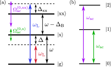
Figure 1: Energy structure of the studied three-level system with external fields. (a) Ground $\lvert\mathrm{g}\rangle$ and two excited levels, $\lvert\mathrm{x}\rangle$ and $\lvert\mathrm{xx}\rangle$, corresponding to the exciton and biexciton in a QD. Acoustic modulation of the excited states is marked with green and violet. Two optical driving cases are marked: $\lvert\mathrm{x}\rangle$ preparation (red arrow) and $\lvert\mathrm{xx}\rangle$ preparation (blue arrow); (b) Dressed-states picture with acoustic field frequencies tuned for $\lvert\mathrm{g}\rangle$–$\lvert\mathrm{x}\rangle$ (green arrow) and $\lvert\mathrm{g}\rangle$–$\lvert\mathrm{xx}\rangle$ (violet arrow) transitions.

We start our considerations by introducing the model of a quantum emitter driven off resonantly by monochromatic laser light with frequency $\omega_{\mathrm{L}}$ and modulated by an acoustic field. We will use two- and three-level system models, where the simpler one will provide us with some intuitive insight, while the quantitative result will come from the three-level model. Fig. 1(a) shows a scheme of considered energy levels. Let us start with two-level systems, where $\lvert\mathrm{g}\rangle$ and $\lvert\mathrm{x}\rangle$ are the ground and excited states (corresponding to no carriers, and an exciton for a QD system) separated by $\hbar\omega$ and coupled by the optical field marked with a red arrow. The acoustic field couples to the excited state, the modulation of which is marked with a green arrow. The Hamiltonian can be written as

$$H(t)=\hbar\omega\rvert\mathrm{x}\rangle\!\langle\mathrm{x}\lvert+\hbar\Omega_{\mathrm{ac}}(t)\rvert\mathrm{x}\rangle\!\langle\mathrm{x}\lvert+\bm{d}\cdot\bm{E}(t),$$ (1)

where $\textit{{E}}(t)=\textit{{E}}_{0}(t)\cos(\omega_{\mathrm{L}}t)$ is the classical optical field, $\bm{d}$ is the dipole moment operator describing the coupling to light. We assume $\langle\mathrm{g}\rvert\bm{d}\lvert\mathrm{g}\rangle=\langle\mathrm{x}\rvert\bm{d}\lvert\mathrm{x}\rangle=0$. Further, $\Omega_{\mathrm{ac}}(t)=\Omega_{\mathrm{ac}}^{(0)}(t)\cos(\omega_{\mathrm{ac}}t)$ is the acoustic field. This Hamiltonian in the rotating wave approximation (RWA) and rotating frame (see Appendix A for derivation) takes the form

$$\begin{split}H(t)&=-\hbar\Delta\rvert\mathrm{x}\rangle\!\langle\mathrm{x}\lvert+\hbar\Omega_{\mathrm{ac}}(t)\rvert\mathrm{x}\rangle\!\langle\mathrm{x}\lvert+\frac{1}{2}\hbar\Omega_{\mathrm{L}}^{(0)}(t)\left(\rvert\mathrm{g}\rangle\!\langle\mathrm{x}\lvert+\rvert\mathrm{x}\rangle\!\langle\mathrm{g}\lvert\right)\\ &=H_{0}+H_{\mathrm{ac}}(t)+H_{\mathrm{L}}(t),\end{split}$$ (2)

where $\Delta=\omega_{\mathrm{L}}-\omega$ is the laser detuning.

For a three-level system with an additional excited state $\lvert\mathrm{xx}\rangle$, see Fig. 1(a) again, we assume that the acoustic field modulates both excited states with different amplitudes due to different coupling strengths. Modulation of the $\lvert\mathrm{xx}\rangle$ state is marked with a violet arrow. We consider no direct optical coupling between the $\lvert\mathrm{g}\rangle$ and $\lvert\mathrm{xx}\rangle$ states. Such a description corresponds to optically active QDs, where $\lvert\mathrm{xx}\rangle$ corresponds to the biexciton state and can be approximately described as a pair of excitons, i.e., a product of orbitally identical exciton states, $\lvert\mathrm{xx}\rangle\approx\lvert\mathrm{x}\rangle\otimes\lvert\mathrm{x}\rangle$. Due to interactions, the biexciton energy is lower than twice the exciton energy by the binding energy $\Delta_{\mathrm{B}}$, for which we choose a typical value of 4 meV. The blue arrow marks the laser, this time detuned by $\Delta_{\mathrm{B}}$ from the $\lvert\mathrm{g}\rangle$–$\lvert\mathrm{xx}\rangle$ transition. The three-level system Hamiltonian in the RWA (see Appendix A for derivation) can be written in the form

$$\begin{split}\!\!\!H(t)=&-\hbar\Delta\rvert\mathrm{x}\rangle\!\langle\mathrm{x}\lvert-\hbar\Delta_{\mathrm{xx}}\rvert\mathrm{xx}\rangle\!\langle\mathrm{xx}\lvert\\ &+\frac{1}{2}\hbar\Omega_{\mathrm{L}}^{(0)}(t)(\rvert\mathrm{x}\rangle\!\langle\mathrm{g}\lvert+\rvert\mathrm{xx}\rangle\!\langle\mathrm{x}\lvert+\mathrm{H.c.})\\ &+\hbar\cos(\omega_{\mathrm{ac}}t)\left(\Omega_{\mathrm{ac}}^{(0,\mathrm{x})}(t)\rvert\mathrm{x}\rangle\!\langle\mathrm{x}\lvert+\Omega_{\mathrm{ac}}^{(0,\mathrm{xx})}(t)\rvert\mathrm{xx}\rangle\!\langle\mathrm{xx}\lvert\right),\end{split}$$ (3)

where $\Omega_{\mathrm{ac}}^{(0,\mathrm{x})}(t)$ and $\Omega_{\mathrm{ac}}^{(0,\mathrm{xx})}(t)$ are the acoustic coupling amplitudes for the two excited states, and $\Delta_{\mathrm{xx}}=2\Delta+\Delta_{\mathrm{B}}$.

We aim to obtain the evolution leading to the full occupation of the $\lvert\mathrm{x}\rangle$ [laser marked with the red arrow in Fig. 1(a)] or $\lvert\mathrm{xx}\rangle$ (blue arrow) state under non-resonant laser driving and with appropriately tuned acoustic modulation. Thanks to sinusoidally varying detunings due to acoustic modulation of excited states’ energies, we should obtain the swing-up behavior when the acoustic frequency matches the respective Rabi frequencies for the system driven by the laser alone, in analogy to the original swing-up concept [36]. The corresponding dressed states, i.e., the new eigenstates of the laser-driven system are schematically shown in Fig. 1(b). The two arrows show the acoustic frequencies that will lead to the occupation of the $\lvert\mathrm{x}\rangle$ (green arrow) and $\lvert\mathrm{xx}\rangle$ (violet) states.

We will study the evolution of the closed system by directly solving the Liouville-von Neumann equation

$$\dot{\rho}(t)=-\frac{i}{\hbar}\left[H(t),\rho(t)\right],$$ (4)

where $\rho(t)$ is the density matrix, for a pure state $\lvert\psi(t)\rangle$ of a closed system defined as $\rho(t)=\rvert\psi(t)\rangle\!\langle\psi(t)\lvert$, with the initial condition given by $\rho(t_{0})=\rvert\mathrm{g}\rangle\!\langle\mathrm{g}\lvert$, i.e., the system initially is prepared in the ground state. The numerical solution of Eq. (4) gives us the exact evolution of a closed system. Further, in Sec. V, we will include the destructive processes, i.e., decoherence due to phonon reaction to the evolution of the system, which will give us achievable fidelity values for states prepared with the acousto-optical scheme.

III Two-level system: exciton preparation

While our final evaluation of state preparation fidelity will be carried out in a three-level system for both $\lvert\mathrm{x}\rangle$ and $\lvert\mathrm{xx}\rangle$ states to keep it realistic, we begin the analysis with a two-level system to provide some intuition and analytical estimates for the needed acoustic field characteristics.

III.1 Tuning the acoustic field

In the case of a two-level system described with Hamiltonian (2), we can find the conditions leading to the desired evolution analytically. To find out, how to choose the acoustic field parameters, we first diagonalize the Hamiltonian $H_{0}+H_{\mathrm{L}}$, i.e., of the system coupled to the laser only. For slowly varying laser pulse envelopes, the transformation is performed at each time point, and yields

$$H_{0}+H_{\mathrm{L}}(t)=E_{+}(t)\rvert+\rangle\!\langle+\lvert+E_{-}(t)\rvert-\rangle\!\langle-\lvert,$$ (5)

where the time-dependent energy difference

$$E_{+}(t)-E_{-}(t)=\hbar\sqrt{\Delta^{2}+\left[\Omega_{\mathrm{L}}^{(0)}(t)\right]^{2}}\equiv\hbar\Omega_{\mathrm{R}}(t)$$ (6)

is now the Rabi frequency of the system described in the basis of states that are dressed by the light,

$$\begin{split}\lvert+(t)\rangle&=\sin\frac{\theta(t)}{2}\lvert\mathrm{g}\rangle+\cos\frac{\theta(t)}{2}\lvert\mathrm{x}\rangle,\\ \lvert-(t)\rangle&=\cos\frac{\theta(t)}{2}\lvert\mathrm{g}\rangle-\sin\frac{\theta(t)}{2}\lvert\mathrm{x}\rangle,\end{split}$$ (7)

where the time-dependent mixing angle $\theta(t)$ is given by

$$\theta(t)=\tan^{-1}\left(\frac{\Omega_{\mathrm{L}}^{(0)}(t)}{\Delta}\right).$$ (8)

The acoustic field Hamiltonian now takes the form

$$\begin{split}H_{\mathrm{ac}}(t)=&\ \hbar\Omega_{\mathrm{ac}}(t)\left(\sin^{2}\frac{\theta(t)}{2}\rvert+\rangle\!\langle+\lvert+\cos^{2}\frac{\theta(t)}{2}\rvert-\rangle\!\langle-\lvert\right)\\ &+\frac{1}{2}\hbar\Omega_{\mathrm{ac}}(t)\sin\theta(t)\left(\rvert+\rangle\!\langle-\lvert+\rvert-\rangle\!\langle+\lvert\right).\end{split}$$ (9)

Having both diagonal and off-diagonal elements, $H_{\mathrm{ac}}$ leads to energy shifts

$$E_{+}(t)\rightarrow E_{+,\mathrm{ac}}(t) =E_{+}(t)+\hbar\Omega_{\mathrm{ac}}(t)\sin^{2}\frac{\theta(t)}{2}$$ (10a)

$$E_{-}(t)\rightarrow E_{-,\mathrm{ac}}(t) =E_{-}(t)+\hbar\Omega_{\mathrm{ac}}(t)\cos^{2}\frac{\theta(t)}{2}$$ (10b)

and, more importantly, transitions between the dressed states. The evolution is thus driven by the off-diagonal terms $\propto\Omega_{\mathrm{ac}}(t)\propto\exp(\pm i\omega_{\mathrm{ac}}t)$. To obtain the resonance condition the frequency $\omega_{\mathrm{ac}}$ has to correspond to the energy difference between the dressed states. Then, we obtain a transition that involves exchanging an energy quantum with the acoustic field,

$$E_{+,\mathrm{ac}}(t)-E_{-,\mathrm{ac}}(t)\pm\hbar\omega_{\mathrm{ac}}=0.$$ (11)

However, the energy difference of the dressed states depends on both time and $\omega_{\mathrm{ac}}$ itself, which leads to a generally nontrivial criterion,

$$\omega_{\mathrm{ac}}(t)=\Omega_{\mathrm{R}}(t)+\Omega_{\mathrm{ac}}(t)\cos\theta(t).$$ (12)

To find a practically feasible condition, we neglect fast oscillations of the dressed states energies and take their mean energy difference as in the original, all-optical swing-up protocol [38]. The resonance condition is then given by

$$\omega_{\mathrm{ac}}(t)=\Omega_{\mathrm{R}}(t).$$ (13)

This condition will hold exactly for flat-top pulses when $\Omega_{\mathrm{R}}$ is constant during the pulse plateau, while some additional optimization around this point will be needed for realistic Gaussian pulses.

III.2 Flat-top pulses

We may carry out fully analytic reasoning for the case of flat-top pulses with the acoustic pulse shorter than the optical one. This situation also corresponds to quasi-continuous optical driving with acoustic pulse triggering the evolution. So, to a case with far-reaching application potential, which may allow the transfer of a quantum state via an acoustic bus. We model flat-top pulses with

$$\Omega_{\eta}^{(0)}(t)=\frac{1}{2}A_{\eta}\left[1-\operatorname{erf}\left(\frac{t-\sigma_{\eta}}{\kappa_{\eta}}\right)\operatorname{erf}\left(\frac{t+\sigma_{\eta}}{\kappa_{\eta}}\right)\right]$$ (14)

for both optical ($\eta=\mathrm{L}$) and acoustic ($\eta=\mathrm{ac}$) fields. Such a pulse has a plateau of duration $\sim\sigma_{\eta}$, and the switching rate is controlled by the $\kappa$ parameter.

The parameter space to explore is large. We choose to fix the laser amplitude equal to detuning so that we do not fall into a regime with Rabi frequency dominated by one of these, i.e., we avoid negligible detunings and situations corresponding to trivial addition of laser and acoustic frequencies. Let $\hbar\Delta=1.75$ meV which is a typical value providing enough spectral separation between the laser and the transition in a QD. For such a case, the needed acoustic field frequency $\hbar\omega_{\mathrm{ac}}\sim 2.3$ meV is almost in the range that is currently experimentally available [42, 43, 44]. In this scenario, we want the optical pulse to be long enough for the acoustic one to operate during the optical plateau. We then have a fixed criterion for the acoustic frequency, $\omega_{\mathrm{ac}}=\Omega_{\mathrm{R}}=\sqrt{\Delta^{2}+A_{\mathrm{L}}^{2}}$. For the protocol to work properly, the acoustic pulse should be long enough for the energy of the oscillating states to average out, i.e., at least a few periods of the acoustic oscillation (we keep it $\gtrsim 5\tau$). Lastly, the optical dressing and undressing of states must be performed quasi-adiabatically. We choose $\sigma_{\mathrm{ac}}=5\tau$, $\kappa_{\mathrm{L}}=2\tau$, $\kappa_{\mathrm{ac}}=\tau$ and $\sigma_{\mathrm{L}}=7\tau$, where $\tau=2\pi/\Omega_{\mathrm{R}}$. The corresponding pulse envelopes are shown in Fig. 2(b).

Now we can fix the amplitude of the acoustic pulse. We want it to cause a $\pi$ rotation in the dressed-state basis, from the $\lvert+\rangle$ to the $\lvert-\rangle$ state. If the entire acoustic pulse occurs during the optical field envelope plateau, we may find the needed acoustic pulse amplitude analytically. In such a situation, the mixing angle $\theta$ Eq. (9) is time-independent, and the effective driving amplitude is $\hbar A_{\mathrm{ac}}\sin\theta/2$ [cf. Eq. (14)]. Thus, for a $\pi$ rotation we need

$$A_{\mathrm{ac}}=\frac{\pi}{\sigma_{\mathrm{ac}}\sin\theta}=\frac{\pi}{\sigma_{\mathrm{ac}}}\sqrt{1+\frac{\Delta^{2}}{A_{\mathrm{L}}^{2}}},$$ (15)

which for our choice of $A_{\mathrm{L}}=\Delta$ gives $\sqrt{2}\pi/\sigma_{\mathrm{ac}}$.

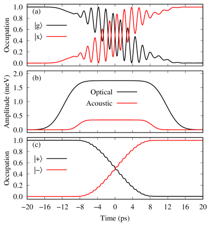
Figure 2: Exciton preparation with flat-top optical coupling pulse and acoustic $\pi$-rotation control pulse: (a) bare states occupations, (b) envelopes of acoustic and optical pulses, (c) occupations of the dressed states. Parameters used: $\hbar\Delta=1.75$ meV, $\hbar A_{\mathrm{L}}=1.75$ meV, $\sigma_{\mathrm{L}}=11.7$ ps, $\hbar A_{\mathrm{ac}}=0.35$ meV, $\sigma_{\mathrm{ac}}=8.36$ ps, $\hbar\omega_{\mathrm{ac}}=2.474$ meV, $\kappa_{\mathrm{L}}=3.34$ ps, and $\kappa_{\mathrm{ac}}=1.67$ ps.

We show the effect of such a pulse in Fig. 2(a) where the system initially prepared in the $\lvert\mathrm{g}\rangle$ state is completely transferred into the $\lvert\mathrm{x}\rangle$ state. As mentioned, the acoustic field envelope satisfies the condition (15) and it is on only during the optical pulse plateau. Thus, it acts only on the states that are already dressed by light, modulating the rotation axis of the qubit periodically. Fig. 2(c) additionally presents the occupation of the dressed states during the evolution. As predicted, the transition is triggered only by the acoustic pulse, which completely transfers the occupation. During switching off the optical field, the state $\lvert-\rangle$ quasi-adiabatically undresses to the excited state.

III.3 Gaussian pulses

For a more realistic simulation, and to explore the case with the reversed role of the fields (optical as a trigger), we now choose a continuous wave acoustic field and a Gaussian optical pulse,

$$\Omega_{\mathrm{ac}}^{(0)}=A_{\mathrm{ac}},\quad\Omega_{\mathrm{L}}^{(0)}(t)=A_{\mathrm{L}}\exp\left(-\frac{t^{2}}{2\sigma_{\mathrm{L}}^{2}}\right).$$ (16)

One should remember that the dressing and undressing procedure has to be adiabatic to fully invert the system occupation, thus the laser pulse cannot be too short. We keep the parameters the same as in the previous subsection.

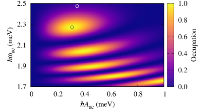
Figure 3: Occupation of the exciton state $\lvert\mathrm{x}\rangle$ as a function of acoustic field parameters for a Gaussian optical pulse ($\hbar\Delta=1.75$ meV, $\hbar A_{\mathrm{L}}=1.75$ meV, $\sigma_{\mathrm{L}}=11.7$ ps) and constant envelope of acoustic driving. We mark a point corresponding to the maximum occupation (black circle), and a point given by analytical prediction [Eq. (13) and Eq. (15)] for flat-top pulses (white circle).

The evolution in this scenario is more complex and some corrections to our analytical predictions from Eq. (13) and Eq. (15) are needed. Thus, we resort to numerical simulations in which we vary $\omega_{\mathrm{ac}}$ and $A_{\mathrm{ac}}$. We again choose $\sigma_{\mathrm{L}}=11.7$ ps, to obtain approximately the same time of the protocol duration. Fig. 3 shows the map of the resultant $\lvert\mathrm{x}\rangle$ state occupation. We achieve full $\pi$-rotation for $\hbar\omega_{\mathrm{ac}}\approx 2.272$ meV and $\hbar A_{\mathrm{ac}}\approx 0.311$ meV, which are close those from Eq. (13) and Eq. (15) for flat-top pulses. The small differences are mainly due to the overlap of the acoustic field with the periods of dressing and the undressing of the states with the optical field when the Gaussian optical pulse does not produce well-defined energy splitting between dressed states. Plugging envelopes from Eq. (16) to the condition in Eq. (12) gives

$$\omega_{\mathrm{ac}}(t)=\Omega_{\mathrm{R}}(t)+A_{\mathrm{ac}}\Delta\frac{\cos(\omega_{\mathrm{ac}}t)}{\Omega_{\mathrm{R}}(t)},$$ (17)

which still averages to $\Omega_{\mathrm{R}}(t)$ over the acoustic oscillation. However, the right-hand side also shows that the effect of acoustic modulation is weaker when $\Omega_{\mathrm{R}}(t)$ is higher [also visible in the driving term in Eq. (9)], which amplifies the contribution of optical pulse tails with lower $\Omega_{\mathrm{R}}(t)$ to the averaged effective $\omega_{\mathrm{ac}}$ needed.

The other visible maxima in Fig. 3 correspond to $3\pi$, $5\pi$, etc. rotations. The shift in the energy is once again caused by the impact of optical pulse tails overlapping with the acoustic field, which is more pronounced for stronger acoustic fields.

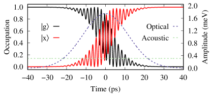
Figure 4: Evolution of bare states occupation in the two-level system during the optical Gaussian pulse coupling and continuous-wave acoustic modulation (left axis) as well as the external field amplitudes (right axis). Acoustic field parameters correspond to the black circle in Fig. 3.

IV Three-level system and biexciton preparation

We now switch to a more realistic three-level model and focus on the biexciton preparation. We start with Eq. (3), where $\Delta_{\mathrm{xx}}=2\Delta+\Delta_{\mathrm{B}}$ is the detuning of twice the laser photon energy from the $\lvert\mathrm{g}\rangle$–$\lvert\mathrm{xx}\rangle$ energy difference. Although there are no direct optical transitions between the ground and biexciton states, we can construct an acousto-optical protocol that allows such transition, again with an analogy with the all-optical swing-up scheme [38]. As previously, we diagonalize the Hamiltonian without the acoustic field, which gives

$$H(t)=E_{0}(t)\rvert 0\rangle\!\langle 0\lvert+E_{1}(t)\rvert 1\rangle\!\langle 1\lvert+E_{2}(t)\rvert 2\rangle\!\langle 2\lvert.$$ (18)

written in the time-dependant dressed states

$$\lvert n(t)\rangle=\!\!\!\sum_{k\in\{\mathrm{g},\mathrm{x},\mathrm{xx}\}}\!\!\!a_{n,k}(t)\lvert k\rangle,$$ (19)

with time-dependent coefficients $a_{n,k}(t)$ dependent on the optical field amplitude and the detuning.

Following the procedure from Sec. III, we add the acoustic field Hamiltonian $H_{\mathrm{ac}}$, which modulates also the biexciton state. We can estimate the strength of this coupling by assuming the biexciton state to be simply a product of exciton states. Then, we have

$$\langle\mathrm{xx}\rvert H_{\mathrm{ac}}\lvert\mathrm{xx}\rangle\approx 2\langle\mathrm{x}\rvert H_{\mathrm{ac}}\lvert\mathrm{x}\rangle,$$ (20)

i.e., the biexciton state is modulated approximately two times stronger than the exciton. Writing $H_{\mathrm{ac}}$ in the $\lvert n(t)\rangle$ basis results again in energy shifts and driving due to the $\propto\rvert n(t)\rangle\!\langle m(t)\lvert$ off-diagonal elements. The resonance condition leading to oscillations between a pair of dressed states is given by

$$\hbar\omega_{\mathrm{ac}}^{(m\leftrightarrow n)}(t)=E_{n}(t)-E_{m}(t).$$ (21)

The new eigenstates of the three-level system are not easy to handle analytically, thus we find the acoustic field parameters needed for the $\pi$-rotation, $\omega_{\mathrm{ac}}$ and $A_{\mathrm{ac}}$, via numerical optimization.

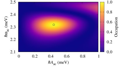
Figure 5: Occupation of the biexciton as a function of acoustic field parameters for a Gaussian optical pulse with ($\hbar\Delta_{\mathrm{xx}}=-2.5$ meV, $\hbar A_{\mathrm{L}}=1.5$ meV, $\sigma_{\mathrm{L}}=11.7$ ps) and constant envelope of acoustic driving. The black circle marks the optimal parameters.

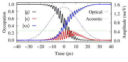
Figure 6: Evolution of state occupations during biexction preparation in the three-level system (left axis) and external field amplitudes (right). The system is driven by an optical Gaussian pulse and continuous-wave acoustic modulation. Acoustic field parameters correspond to the black circle in Fig. 5.

We again consider a non-resonant Gaussian optical pulse during a constant acoustic driving [Eq. (16)]. In Fig. 5, we scan the acoustic field frequency and amplitude to find the optimal parameters. The higher, $(2n+1)\pi$ rotations this time occur for significantly larger acoustic field amplitudes than in the exciton occupation protocol and we do not show them here. The optimal parameters are $\hbar\omega_{\mathrm{ac}}=2.318$ meV, and $\hbar A_{\mathrm{ac}}=0.443$ meV. We choose $\Delta_{\mathrm{xx}}=-2.5$ meV, and $\hbar A_{\mathrm{L}}=1.5$ meV, which do not fully correspond to the parameters studied for the two-level system, but the frequency of the acoustic field remains similar as in the previous section. In this case, the acoustic field amplitude matches the one we needed to prepare the exciton state, but the energy scale is different. No optical coupling between ground and biexciton states and coupling of both these states to $\lvert\mathrm{x}\rangle$ results in lower splitting of the corresponding dressed states and thus lower Rabi frequency.

V Phonon-induced decoherence

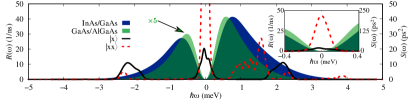
Figure 7: Spectral functions calculated for $T=20$ K. The solid black line and dotted red line are nonlinear spectral characteristics $S(\omega)$ calculated for exciton and biexciton preparation respectively. Blue- and green-shaded areas show spectral densities for InAs/GaAs and GaAs/AlGaAs QDs, respectively. Values for GaAs QDs are low and are scaled $5\times$ for visibility. Note that the central peak in $S(\omega)$ extends beyond the right $y$-axis range, which is chosen narrow to better show the lower side peaks, while the inset repeats the central part of the graph to show those peaks around $\omega=0$.

The evolution of a real system differs from the idealized one studied above. First, there is the obvious impact of the radiative recombination from the exciton and biexciton states, which forces one to prepare the state in a period much shorter than the recombination time. A more subtle effect arises due to the presence of a phonon environment. As both exciton and biexciton states couple to deformations, phonons can dynamically react to the evolution of charge states in a QD [45]. This reaction results in the creation of system-bath entanglement and, in turn, in the decoherence of QD states. This process is non-Markovian and requires careful treatment. Below, we work in the second-order Born approximation to estimate the fidelity $F$ of the prepared states by calculating the post-protocol difference of density matrices from unperturbed evolution and the one including phonon response. For this, we follow the approach from Ref. [45], which we also outline in Appendix B.

$T$ (K)	Prepared state	Fidelity (%)
		GaAs/AlGaAs QDs	InAs/GaAs QDs
4		99.70	96.41
10		99.50	95.27
20	$\lvert\mathrm{x}\rangle$	99.11	92.18
77		96.68	68.29
300		86.40
4		98.07	83.80
10		97.25	78.01
20	$\lvert\mathrm{xx}\rangle$	95.59	63.61
77		84.94
300

Table 1: Fidelity of the exciton $\lvert\text{x}\rangle$ and biexciton $\lvert\text{xx}\rangle$ states prepared with Gaussian optical pulses and continuous-wave acoustic modulation, calculated for InAs/GaAs and GaAs/AlGaAs QDs at different temperatures. In all cases, calculations are done within the three-level model.

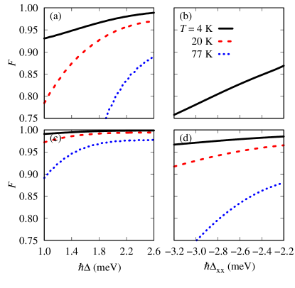
Figure 8: Achievable fidelity as a function of the laser detuning. The top row corresponds to InAs/GaAs QDs and the bottom row to GaAs/AlGaAs QDs. The left column stands for the exciton preparation and the right column for the biexciton case.

To relate our study to existing and application-relevant platforms, we consider two types of semiconductor QDs: standard self-assembled InAs/GaAs QDs and GaAs/Al_0.4Ga_0.6As QDs grown by droplet etching epitaxy. Details of the calculation and QD modeling are given in Appendix C. We calculate the fidelity for the cases of exciton and biexciton preparation with Gaussian optical pulses during continuous-wave acoustic modulation (and not vice-versa), which is the one more prone to be non-ideal due to temporal overlaps of acoustic modulation with (un)dressing of states with light. We show the fidelity values in Table 1. In all cases, we find high quality of the prepared states at low temperatures. For InAs/GaAs QDs, we may notice a deterioration with increasing temperature due to a significant increase in phonon occupations. GaAs/AlGaAs QDs show excellent fidelity values at cryogenic temperatures for both exciton and biexciton preparation and even fidelity exceeding $85\%$ at room temperature for exciton preparation. However, this result takes into account only the evolution of the three-level system and the resultant phonon impact. We thus show the room temperature results in gray to underline their limited reliability, as, especially in large-volume GaAs QDs, thermal excitations to higher orbital states play a role in the evolution at such elevated temperatures [46]. Nonetheless, for appropriately selected detuning the protocol itself proves to be almost decoherence-free in terms of dynamical phonon-induced effects, in agreement with recent findings for the all-optical implementation [37, 47].

The decoherence strength can be understood based on its physical origin due to the dynamical phonon response to the evolution of charges (polaron formation), entangling the system with the environment. One can decompose this evolution into contributions with different frequencies, which is described by the nonlinear spectral function $S(\omega)$ (see Appendix B for definition). Phonons can respond only at a limited range of frequencies, and their frequency-dependent response strength is described with spectral density $R(\omega)$ (see Appendix B again), which depends also on the geometry of confined charge states. The loss of fidelity is given by the overlap between those two spectral functions. We presented them in Fig. 7. The spectral densities for the two kinds of QDs are plotted for $T=20$ K, and $S(\omega)$ is shown for both exciton (solid black line) and biexciton (dotted red line) preparation. Solid and dotted lines show the nonlinear spectral functions for preparation of $\lvert\mathrm{x}\rangle$ and $\lvert\mathrm{xx}\rangle$, respectively. One may notice multiple peaks over a wide range of frequencies (energy), with a much richer $S(\omega)$ spectrum for the biexciton preparation protocol. The multiple peaks in the range from $0.75$ meV to $2$ meV correspond to the transitions between exciton and biexciton states during the evolution. Phonon spectral densities are shown with filled curves. They strongly depend on the QD geometry and $R(\omega)$ is much wider and higher for small InAs/GaAs QDs compared to the large-volume GaAs/AlGaAs QDs. Thus, it catches a larger set of frequencies present in the system evolution, lowering the value of the fidelity. The rest of the visible peaks can be assigned to the unitary evolution of the states and the acoustic field frequency.

Finally, we can study the dependence of achievable fidelity on laser detuning with the results for three selected temperatures shown in Fig. 8. The top row of panels corresponds to GaAs QDs and the bottom one is for the InAs QDs, while columns show results for different prepared states in the protocol. The fidelity of preparing the exciton state behaves as one could predict. While increasing the detuning, the overlap between spectral functions becomes smaller, because the evolution is driven by higher frequencies for which the phonon response is weaker, thus the fidelity increases. The temperature increases the number of phonons that entangle with the qubit, increasing the error of the protocol. In the case of the biexciton preparation, one of the main frequencies in the evolution is the one between exciton and biexciton. Thus, increasing the absolute value of the detuning causes this transition energy to decrease, increasing the overlap between spectral functions. On the other hand, decreasing the absolute value of this detuning below $2.2$ meV causes difficulties due to the mixing of the exciton and biexciton states.

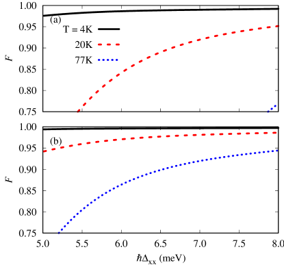
Figure 9: Achievable fidelity of the biexciton state preparation as a function of the laser detuning. The top row corresponds to InAs/GaAs QDs and the bottom row to GaAs/AlGaAs QDs. The range of needed acoustic field energies is from $5.8$ meV to $8.2$ meV.

As can be noticed in Fig. 8, the fidelity of the biexciton state preparation is significantly lower than for the exciton case for currently achievable sub-THz phonon frequencies. We perform additional simulations to show that our biexciton state preparation can achieve very high fidelity even at the liquid nitrogen temperature when terahertz acoustic frequencies become available. In Fig. 9, we show the fidelity for larger detunings corresponding to driving with acoustic fields with the phonon energy in the $5.8$–$8.2$ meV range. In this case, we predict a significant increase in the fidelity for both types of QDs. For InAs QDs (Fig. 9(a)) it exceeds $95\%$ at $T=20$ K, and $75\%$ at $T=77$ K (fidelity can be further increased, increasing the detuning), while at lower detunings [Fig. 8] the phonon impact was even beyond the perturbative regime. For GaAs QDs [Fig. 9(b)] we observe a qualitatively similar behavior of fidelity as previously, but with even higher values. At $T=4$ K the biexciton preparation is almost decoherence-free ($F>99.7\%$), and at higher temperatures, we also find significantly improved fidelity compared to the sub-THz acoustic modulation.

VI Conclusions

We have proposed a new hybrid acousto-optical method for the preparation of exciton and biexciton states in quantum emitters including semiconductor QDs. The method is based on the recently introduced swing-up scheme, which had an all-optical implementation. Here, we propose to use the acoustic field to modulate the detuning in resonance with the Rabi frequency under off-resonant optical driving. This leads to the periodic oscillations of the qubit rotation axis enabling the swing-up behavior of the system. Our scheme is adequate for both positive and negative detunings, with the only limitation caused by the availability of needed acoustic field frequencies. In agreement with similar evaluations for the all-optical implementation, we have found the scheme to be almost phonon decoherence-free even at elevated temperatures. The direct acoustic modulation of the detuning eliminates the need for precise control of two optical pulses present in the original all-optical swing-up implementation. More importantly, the scheme can use the acoustic pulse as a trigger for the transition and hence may pave the way for generating entanglement between the emitter and a quantum acoustic mode, leading to subsequent state transfer via an acoustic bus.

Appendix A Rotating wave approximation

We consider a three-level atomic-like system with the ground level $\lvert\mathrm{g}\rangle$ and two excited states $\lvert\mathrm{x}\rangle$ and $\lvert\mathrm{xx}\rangle$. In a QD, those states stand for an empty QD, the exciton state, and the biexciton state respectively. Let the $\hbar\omega$ be the transition energy between $\lvert\mathrm{g}\rangle$ and $\lvert\mathrm{x}\rangle$ states, and $\hbar\omega-\hbar\Delta_{\mathrm{B}}$ between the $\lvert\mathrm{x}\rangle$ and $\lvert\mathrm{xx}\rangle$. Then, the Hamiltonian can be written as

$$H_{0}=\hbar\omega\rvert\mathrm{x}\rangle\!\langle\mathrm{x}\lvert+\hbar(2\omega-\Delta_{\mathrm{B}})\rvert\mathrm{xx}\rangle\!\langle\mathrm{xx}\lvert.$$ (22)

Let the QD interact with an external optical field with frequency $\omega_{\mathrm{L}}$. In the dipole approximation the interaction Hamiltonian can be expressed as

$$H_{\mathrm{int}}(t)=\bm{d}\cdot\bm{E}(t),$$ (23)

where $\bm{d}$ is the dipole moment operator. Assuming no diagonal coupling between laser and QD states, and appropriate linear polarization of the optical field, we can write the full Hamiltonian $H_{0}+H_{\mathrm{int}}$ in the form

$$\begin{split}H(t)=&\ \hbar\omega\rvert\mathrm{x}\rangle\!\langle\mathrm{x}\lvert+\hbar\left(2\omega-\Delta_{\mathrm{B}}\right)\rvert\mathrm{xx}\rangle\!\langle\mathrm{xx}\lvert\\ &+\hbar\Omega_{\mathrm{L}}(t)\left(\rvert\mathrm{x}\rangle\!\langle\mathrm{g}\lvert+\rvert\mathrm{x}\rangle\!\langle\mathrm{xx}\lvert+\mathrm{H.c.}\right),\end{split}$$ (24)

where $\Omega_{\mathrm{L}}(t)=\Omega_{\mathrm{L}}^{(0)}(t)\cos(\omega_{\mathrm{L}}t)$ is a classical optical field. Next, we perform a unitary transformation to a rotating frame with $U(t)=e^{S(t)}$ given by

$$S(t)=i\omega t\rvert\mathrm{x}\rangle\!\langle\mathrm{x}\lvert+2i\omega t\rvert\mathrm{xx}\rangle\!\langle\mathrm{xx}\lvert.$$ (25)

The transformed Hamiltonian is

$$\widetilde{H}(t)=U(t)H(t)U^{\dagger}(t)+i\hbar\dot{U}(t)U^{\dagger}(t),$$ (26)

which gives us

$$\begin{split}\widetilde{H}(t)=&\ \hbar\left(\omega-\omega_{\mathrm{L}}\right)\rvert\mathrm{x}\rangle\!\langle\mathrm{x}\lvert+\hbar\left(2\omega-2\omega_{\mathrm{L}}-\Delta_{\mathrm{B}}\right)\rvert\mathrm{xx}\rangle\!\langle\mathrm{xx}\lvert\\ &+\frac{1}{2}\hbar\Omega_{\mathrm{L}}^{(0)}(t)\left(e^{i\omega_{\mathrm{L}}t}+e^{-i\omega_{\mathrm{L}}t}\right)\\ &\phantom{+~{}}\times\left(e^{i\omega_{\mathrm{L}}t}\rvert\mathrm{x}\rangle\!\langle\mathrm{g}\lvert+e^{-i\omega_{\mathrm{L}}t}\rvert\mathrm{x}\rangle\!\langle\mathrm{xx}\lvert+\mathrm{H.c.}\right).\end{split}$$ (27)

The terms $\propto\exp{(\pm 2i\omega_{\mathrm{L}}t)}$ can be neglected due to fast oscillating behavior. This step is called the rotating wave approximation. The difference $\omega_{\mathrm{L}}-\omega=\Delta$ is the detuning of the optical field from the $\lvert\mathrm{g}\rangle-\lvert\mathrm{x}\rangle$ transition. Finally, the Hamiltonian in the dipole and RWA approximations reads

$$\begin{split}\widetilde{H}(t)=&\ -\hbar\Delta\rvert\mathrm{x}\rangle\!\langle\mathrm{x}\lvert-\hbar(2\Delta+\Delta_{\mathrm{B}})\rvert\mathrm{xx}\rangle\!\langle\mathrm{xx}\lvert\\ &+\frac{1}{2}\hbar\Omega_{\mathrm{L}}^{(0)}(t)(\rvert\mathrm{x}\rangle\!\langle\mathrm{g}\lvert+\rvert\mathrm{x}\rangle\!\langle\mathrm{xx}\lvert+\mathrm{H.c.}).\end{split}$$ (28)

Appendix B Fidelity calculation

Let the isolated carrier subsystem be described by Hamiltonian $H_{\mathrm{S}}=\sum_{i}E_{i}\rvert i\rangle\!\langle i\lvert$. In the non-perturbed case, the unitary evolution of the entire system composed of the studied subsystem and its phonon bath is given by

$$U_{0}(t)=U(t)\otimes e^{-iH_{\mathrm{ph}}t/\hbar},$$ (29)

where $U(t)=\exp({-iH_{\mathrm{S}}t/\hbar})$ is the unitary evolution operator of the carrier subsystem in the absence of the carrier-phonon interaction, and the $H_{\mathrm{ph}}$ is the free phonon Hamiltonian. The interaction between carriers and phonons can always be written in the general form

$$V=\sum_{nm}S_{nm}\otimes R_{nm},$$ (30)

where $S_{nm}=\rvert n\rangle\!\langle m\lvert$ acts in the Hilbert space of the carrier subsystem and

$$R_{nm}=\sum_{\bm{k}}F_{nm}(\bm{k})(b_{\bm{k}}+b_{-\bm{k}}^{\dagger})$$ (31)

acts only on the phonon environment. Here $b_{\bm{k}}$ and $b_{\bm{k}}^{\dagger}$ are the annihilation and creation operators for phonons in a mode labeled by $\bm{k}$.

We assume that the carrier system is initially in a product state

$$\varrho(t_{0})=\rho_{0}\otimes\rho_{\mathrm{R}}$$ (32)

where $\rho_{0}=\rvert\psi_{0}\rangle\!\langle\psi_{0}\lvert$ is the initial system density matrix and $\rho_{\mathrm{R}}$ is the phonon density matrix in the thermal equilibrium.

The evolution of the full density matrix $\varrho(t)$ is given by the Liouville-von Neumann equation

$$\dot{\varrho}(t)=-\frac{i}{\hbar}[H_{\mathrm{S}}+H_{\mathrm{ph}}+V,\varrho(t)].$$ (33)

We are interested in the evolution of the reduced density matrix of the carrier subsystem, $\rho(t)=\mathrm{Tr}_{\mathrm{R}}\varrho(t)$, where $\mathrm{Tr}_{\mathrm{R}}$ is the trace over the environmental degrees of freedom. We assume that the influence of the environment is weak so that the reduced density matrix has the form

$$\rho(t)=\rho^{(0)}(t)+\Delta\rho(t),$$ (34)

where $\Delta\rho(t)$ is the phonon-induced correction to the unperturbed evolution $\rho^{(0)}(t)=U(t)\rho_{0}U^{\dagger}(t)$. To quantify the quality of preparation of the given carrier state, we use fidelity, which is a measure of the overlap between final ($t\to\infty$) states with and without perturbation. It is given by

$$\begin{split}F^{2}&=\langle\psi_{0}\rvert U_{0}^{\dagger}(\infty)\rho(\infty)U_{0}(\infty)\lvert\psi_{0}\rangle\\ &=1+\langle\psi_{0}\rvert\Delta\tilde{\rho}(\infty)\lvert\psi_{0}\rangle,\end{split}$$ (35)

where $\Delta\tilde{\rho}(\infty)$ is the perturbation in the interaction picture at the end of the protocol and it is calculated in the second-order Born approximation,

$$\Delta\tilde{\rho}(t)=-\frac{1}{\hbar^{2}}\int_{t_{0}}^{t}\mathrm{d}\tau\int_{t_{0}}^{\tau}\mathrm{d}\tau^{\prime}\mathrm{Tr}_{\mathrm{R}}[\tilde{V}(\tau),[\tilde{V}(\tau^{\prime}),\varrho(t_{0})]],$$ (36)

where $\tilde{V}(\tau)$ is $V$ written in the interaction picture. At this stage, it is convenient to introduce two types of spectral functions. The first is the spectral density of the reservoir

$$R_{ijkl}(\omega)=\frac{1}{2\pi}\int\mathrm{d}t\langle R_{ij}(t)R_{kl}\rangle e^{i\omega t},$$ (37)

where the operator $R_{ij}(t)$ is transformed into the interaction picture. The second spectral function is the nonlinear spectral characteristic, defined as

$$S_{ijkl}(\omega)=\sum_{n}\langle\psi_{0}\rvert Y^{\dagger}_{ij}(\omega)\rvert\psi_{n}\rangle\!\langle\psi_{n}\lvert Y_{kl}(\omega)\lvert\psi_{0}\rangle,$$ (38)

where the set of vectors $\lvert\psi_{n}\rangle$ spans the space orthogonal to the initial state. The functions $Y_{ij}(\omega)$ are defined as

$$Y_{ij}(\omega)=\int_{t_{0}}^{t}\mathrm{d}\tau S_{ij}(\tau)e^{-i\omega\tau},$$ (39)

where $S_{ij}(t)=U_{0}^{\dagger}(t)S_{ij}U_{0}(t)$. Using the above equations the fidelity can be written in the form

$$F^{2}=1-\sum_{ijkl}\int\mathrm{d}\omega R_{ijkl}(\omega)S_{ijkl}(\omega).$$ (40)

Appendix C Phonon induced decoherence in the three-level model of a QD

To simplify Eq. (40) in our system, we can introduce the interaction with phonons in the form

$$V=(\rvert\mathrm{x}\rangle\!\langle\mathrm{x}\lvert+2\rvert\mathrm{xx}\rangle\!\langle\mathrm{xx}\lvert)\otimes R_{\mathrm{xx}},$$ (41)

where we use the fact that the biexciton-phonon coupling is approximately two times stronger than for the exciton. Thanks to this, we reduce the number of spectral densities to one, and this allows us to omit summations in Eq. (40). The corresponding spectral density $R(\omega)$ is given by

$$R(\omega)=\frac{\mathcal{V}|n(\omega)+1|}{(2\pi)^{3}\hbar^{2}}\sum_{\lambda}\int_{\mathbb{R}^{3}}\mathrm{d}^{3}\bm{k}\left|g_{\bm{k,\lambda}}\right|^{2}\delta(|\omega|-\omega_{\bm{k},\lambda}),$$ (42)

where $\mathcal{V}$ is the phonon mode normalization volume, $n(\omega)$ is the Bose-Einstein distribution, and the coupling $g_{\bm{k,\lambda}}$ between phonons and an electron-hole pair

$$g_{\bm{k,\lambda}}=g_{\bm{k,\lambda}}^{(\mathrm{e,DP})}+g_{\bm{k,\lambda}}^{(\mathrm{e,PE})}+g_{\bm{k,\lambda}}^{(\mathrm{h,DP})}+g_{\bm{k,\lambda}}^{(\mathrm{h,PE})}$$ (43)

contains couplings by piezoelectric effect (PE) and deformation potential (DP). From now on we also replace the generic $\bm{k}$ labeling phonon modes with the proper phonon wave vector $\bm{k}$ and branch (polarization) $\lambda$ with three values, LA, TA1, TA2 corresponding to longitudinal, and two transverse acoustic branches. We also assume linear phonon dispersion $\omega_{\bm{k},\lambda}=c_{\lambda}k$, where $c_{\lambda}$ is the sound velocity in the material. The coupling constants can be written as

$$g_{\bm{k,\lambda}}^{(\mathrm{e/h,DP})}=a_{c/v}\sqrt{\frac{\hbar k}{2d\mathcal{V}c_{\mathrm{\lambda}}}}\mathcal{F}_{\mathrm{e/h}}(\bm{k})\delta_{\lambda,\mathrm{LA}},$$ (44a)

$$g_{\bm{k,\lambda}}^{(\mathrm{e/h,PE})}=\pm i\frac{ee_{14}}{\varepsilon_{0}\varepsilon_{r}}\sqrt{\frac{\hbar}{2d\mathcal{V}\omega_{\bm{k},\lambda}}}M_{\lambda}(\bm{k})\mathcal{F}_{\mathrm{e/h}}(\bm{k}),$$ (44b)

where

$$\mathcal{F}_{\mathrm{e/h}}(\bm{k})=\int_{\mathbb{R}^{3}}\mathrm{d}^{3}\bm{r}\,\varPsi^{*}_{\mathrm{e/h}}(\bm{r})\varPsi_{\mathrm{e/h}}(\bm{r})e^{i\bm{k}\cdot\bm{r}}$$ (45)

is the form factor that contains all information about the system via the electron/hole ground-state wave functions $\varPsi_{\mathrm{e/h}}(\bm{r})$, and $M_{\lambda}(\bm{k})$ is a function that depends on the orientation of the phonon wave vector [48] and in the spherical coordinates takes the form

$$\begin{split}M_{\mathrm{LA}}&=\frac{3}{2}\sin 2\vartheta\cos\vartheta\sin 2\phi,\\ M_{\mathrm{T}1}&=\sin 2\vartheta\cos 2\phi,\\ M_{\mathrm{T}2}&=(3\sin^{2}\vartheta-1)\cos\vartheta\sin 2\phi.\end{split}$$ (46)

For a QD we assume standard Gaussian shapes of the wave functions $\varPsi_{\mathrm{e/h}}(\bm{r})$ are given by product $\varPsi_{\mathrm{e/h}}(\bm{r})=\Pi_{i}\psi_{i}^{(\mathrm{e/h})}(x_{i})$, where

$$\psi_{i}^{(\mathrm{e})}(x_{i})=\frac{1}{\sqrt{2\pi}l_{i}}e^{\frac{-x_{i}^{2}}{2l_{i}^{2}}}$$ (47)

is the wave function of the carrier in the direction $x_{i}$ with the extension given by $l_{i}$. We assume stronger hole localization compared to the electron, i.e., $l_{i}^{(\mathrm{h})}=0.8l_{i}^{(\mathrm{e})}$.

	InAs/GaAs	GaAs/AlGaAs
$a_{c}$ (eV)	-7.17	-6.558
$a_{v}$ (eV)	-1.16	-0.292
$d$ (kg/$\mathrm{m}^{3}$)	5350	4698
$c_{\mathrm{LA}}$ (m/s)	4730	5530
$e_{14}$ mC/$(\mathrm{m}^{2})$	-160	-145
$\varepsilon_{r}$	12.9	11.42
Wave-function extension $l$:
in-plane (nm)	6	9
$z$-axis (nm)	2	3

Table 2: Material parameters used to calculate spectral densities taken from Refs. 49, 50, 51. The parameters of AlGaAs were calculated using a linear interpolation between the AlAs and GaAs parameters. Material parameters refer to the barrier materials, as we consider bulk phonons.

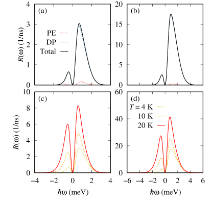
Figure 10: Phonon spectral densities: (a) Contribution of piezoelectric effect (PE), deformation potential (DP), and total spectral density for GaAs/AlGaAs QDs calculated at $T=4$ K, (b) the same as (a) but for InAs/GaAs QDs, (c) Temperature dependence for GaAs/AlGaAs QDs, (d) Temperature dependence for InAs/GaAs QDs.

The material parameters used to calculate phonon spectral densities are shown in Table 2. Spectral densities for the two types of studied QDs and the contributions of PE and DP couplings at a low temperature of 4 K are shown in Fig. 10(a) and Fig. 10(b). The temperature dependence is presented in Fig. 10(c) and Fig. 10(d).

References

- Kurizki et al. [2015] G. Kurizki, P. Bertet, Y. Kubo, K. Mølmer, D. Petrosyan, P. Rabl, and J. Schmiedmayer, Proc. Natl. Acad. Sci. 112, 3866 (2015).
- Morton and Lovett [2011] J. J. Morton and B. W. Lovett, Annu. Rev. Conden. Ma. P. 2, 189 (2011).
- Wallquist et al. [2009] M. Wallquist, K. Hammerer, P. Rabl, M. Lukin, and P. Zoller, Phys. Scripta 2009, 014001 (2009).
- Xiang et al. [2013] Z.-L. Xiang, S. Ashhab, J. Q. You, and F. Nori, Rev. Mod. Phys. 85, 623 (2013).
- Daniilidis et al. [2013] N. Daniilidis, D. J. Gorman, L. Tian, and H. Häffner, New J. Phys. 15, 073017 (2013).
- Aspelmeyer et al. [2014] M. Aspelmeyer, T. J. Kippenberg, and F. Marquardt, Rev. Mod. Phys. 86, 1391 (2014).
- Helstrom [1969] C. W. Helstrom, J. Stat. Phys. 1, 231 (1969).
- Tucker and Feldman [1985] J. R. Tucker and M. J. Feldman, Rev. Mod. Phys. 57, 1055 (1985).
- Pezzè [2021] L. Pezzè, Nat. Photonics 15, 74 (2021).
- Langbein and Patton [2006] W. Langbein and B. Patton, Opt. Lett. 31, 1151 (2006).
- Unitt et al. [2005] D. C. Unitt, A. J. Bennett, P. Atkinson, K. Cooper, P. See, D. Gevaux, M. B. Ward, R. M. Stevenson, D. A. Ritchie, and A. J. Shields, J. Opt. B 7, S129 (2005).
- Michler et al. [2000] P. Michler, A. Kiraz, C. Becher, W. V. Schoenfeld, P. M. Petroff, L. Zhang, E. Hu, and A. Imamoglu, Science 290, 2282 (2000).
- Santori et al. [2001] C. Santori, M. Pelton, G. Solomon, Y. Dale, and Y. Yamamoto, Phys. Rev. Lett. 86, 1502 (2001).
- Ding et al. [2016] X. Ding, Y. He, Z.-C. Duan, N. Gregersen, M.-C. Chen, S. Unsleber, S. Maier, C. Schneider, M. Kamp, S. Höfling, C.-Y. Lu, and J.-W. Pan, Phys. Rev. Lett. 116, 020401 (2016).
- Chekhovich et al. [2020] E. A. Chekhovich, S. F. C. da Silva, and A. Rastelli, Nat. Nanotech. 15, 999 (2020).
- Vajner et al. [2022] D. A. Vajner, L. Rickert, T. Gao, K. Kaymazlar, and T. Heindel, Adv. Quantum Technol. 5, 2100116 (2022).
- Schimpf et al. [2021] C. Schimpf, M. Reindl, D. Huber, B. Lehner, S. F. C. D. Silva, S. Manna, M. Vyvlecka, P. Walther, and A. Rastelli, Sci. Adv. 7, eabe8905 (2021).
- Hafenbrak et al. [2007] R. Hafenbrak, S. M. Ulrich, P. Michler, L. Wang, A. Rastelli, and O. G. Schmidt, New J. Phys. 9, 315 (2007).
- Huber et al. [2018] D. Huber, M. Reindl, J. Aberl, A. Rastelli, and R. Trotta, J. Opt. 20, 073002 (2018).
- Stievater et al. [2001] T. H. Stievater, X. Li, D. G. Steel, D. Gammon, D. S. Katzer, D. Park, C. Piermarocchi, and L. J. Sham, Phys. Rev. Lett. 87, 133603 (2001).
- Kamada et al. [2001] H. Kamada, H. Gotoh, J. Temmyo, T. Takagahara, and H. Ando, Phys. Rev. Lett. 87, 246401 (2001).
- Ramsay [2010] A. J. Ramsay, Semicond. Sci. Tech. 25, 103001 (2010).
- Simon et al. [2011] C.-M. Simon, T. Belhadj, B. Chatel, T. Amand, P. Renucci, A. Lemaitre, O. Krebs, P. A. Dalgarno, R. J. Warburton, X. Marie, and B. Urbaszek, Phys. Rev. Lett. 106, 166801 (2011).
- Wu et al. [2011] Y. Wu, I. M. Piper, M. Ediger, P. Brereton, E. R. Schmidgall, P. R. Eastham, M. Hugues, M. Hopkinson, and R. T. Phillips, Phys. Rev. Lett. 106, 067401 (2011).
- Lüker and Reiter [2019] S. Lüker and D. E. Reiter, Semicond. Sci. Tech. 34, 063002 (2019).
- Thomas et al. [2021] S. E. Thomas, M. Billard, N. Coste, S. C. Wein, Priya, H. Ollivier, O. Krebs, L. Tazaïrt, A. Harouri, A. Lemaitre, I. Sagnes, C. Anton, L. Lanco, N. Somaschi, J. C. Loredo, and P. Senellart, Phys. Rev. Lett. 126, 233601 (2021).
- Vyvlecka et al. [2023] M. Vyvlecka, L. Jehle, C. Nawrath, F. Giorgino, M. Bozzio, R. Sittig, M. Jetter, S. L. Portalupi, P. Michler, and P. Walther, Appl. Phys. Lett. 123, 174001 (2023).
- Kaldewey et al. [2017] T. Kaldewey, S. Lüker, A. V. Kuhlmann, S. R. Valentin, J.-M. Chauveau, A. Ludwig, A. D. Wieck, D. E. Reiter, T. Kuhn, and R. J. Warburton, Phys. Rev. B 95, 241306 (2017).
- Mathew et al. [2014] R. Mathew, E. Dilcher, A. Gamouras, A. Ramachandran, H. Y. S. Yang, S. Freisem, D. Deppe, and K. C. Hall, Phys. Rev. B 90, 035316 (2014).
- He et al. [2019] Y.-M. He, H. Wang, C. Wang, M.-C. Chen, X. Ding, J. Qin, Z.-C. Duan, S. Chen, J.-P. Li, R.-Z. Liu, C. Schneider, M. Atatüre, S. Höfling, C.-Y. Lu, and J.-W. Pan, Nat. Phys. 15, 941 (2019).
- Koong et al. [2021] Z. X. Koong, E. Scerri, M. Rambach, M. Cygorek, M. Brotons-Gisbert, R. Picard, Y. Ma, S. I. Park, J. D. Song, E. M. Gauger, and B. D. Gerardot, Phys. Rev. Lett. 126, 047403 (2021).
- Matthiesen et al. [2012] C. Matthiesen, A. N. Vamivakas, and M. Atatüre, Phys. Rev. Lett. 108, 093602 (2012).
- Kuhlmann et al. [2013] A. V. Kuhlmann, J. Houel, D. Brunner, A. Ludwig, D. Reuter, A. D. Wieck, and R. J. Warburton, Rev. Sci. Instrum. 84, 073905 (2013).
- Ardelt et al. [2014] P.-L. Ardelt, L. Hanschke, K. A. Fischer, K. Müller, A. Kleinkauf, M. Koller, A. Bechtold, T. Simmet, J. Wierzbowski, H. Riedl, G. Abstreiter, and J. J. Finley, Phys. Rev. B 90, 241404 (2014).
- Barth et al. [2016] A. M. Barth, S. Lüker, A. Vagov, D. E. Reiter, T. Kuhn, and V. M. Axt, Phys. Rev. B 94, 045306 (2016).
- Bracht et al. [2021] T. K. Bracht, M. Cosacchi, T. Seidelmann, M. Cygorek, A. Vagov, V. M. Axt, T. Heindel, and D. E. Reiter, PRX Quantum 2, 040354 (2021).
- Bracht et al. [2022] T. K. Bracht, T. Seidelmann, T. Kuhn, V. M. Axt, and D. E. Reiter, Phys. Status Solidi B 259, 2100649 (2022).
- Bracht et al. [2023a] T. K. Bracht, T. Seidelmann, Y. Karli, F. Kappe, V. Remesh, G. Weihs, V. M. Axt, and D. E. Reiter, Phys. Rev. B 107, 035425 (2023a).
- Karli et al. [2022] Y. Karli, F. Kappe, V. Remesh, T. K. Bracht, J. Münzberg, S. Covre da Silva, T. Seidelmann, V. M. Axt, A. Rastelli, D. E. Reiter, and G. Weihs, Nano Lett. 22, 6567 (2022).
- Boos et al. [2022] K. Boos, F. Sbresny, S. K. Kim, M. Kremser, H. Riedl, F. W. Bopp, W. Rauhaus, B. Scaparra, K. D. Jöns, J. J. Finley, K. Müller, and L. Hanschke, Coherent dynamics of the swing-up excitation technique (2022), arXiv:2211.14289 [quant-ph] .
- da Silva et al. [2021] S. F. C. da Silva, G. Undeutsch, B. Lehner, S. Manna, T. M. Krieger, M. Reindl, C. Schimpf, R. Trotta, and A. Rastelli, Appl. Phys. Lett. 119, 120502 (2021).
- Poyser et al. [2015] C. L. Poyser, A. V. Akimov, R. P. Campion, and A. J. Kent, Scientific Reports 5, 8279 (2015).
- Akimov et al. [2015] A. Akimov, A. Scherbakov, D. Yakovlev, and M. Bayer, Ultrasonics 56, 122 (2015).
- Ruello and Gusev [2015] P. Ruello and V. E. Gusev, Ultrasonics 56, 21 (2015).
- Roszak et al. [2005] K. Roszak, A. Grodecka, P. Machnikowski, and T. Kuhn, Phys. Rev. B 71, 195333 (2005).
- Lehner et al. [2023] B. U. Lehner, T. Seidelmann, G. Undeutsch, C. Schimpf, S. Manna, M. Gawełczyk, S. F. Covre da Silva, X. Yuan, S. Stroj, D. E. Reiter, V. M. Axt, and A. Rastelli, Nano Lett. 23, 1409 (2023).
- Bracht et al. [2023b] T. K. Bracht, M. Cygorek, T. Seidelmann, V. M. Axt, and D. E. Reiter, Optica Quantum 1, 103 (2023b).
- Mahan [2000] G. D. Mahan, Many-Particle Physics (Physics of Solids and Liquids) (Springer, Berlin, 2000).
- Tse et al. [2013] G. Tse, J. Pal, U. Monteverde, R. Garg, V. Haxha, M. A. Migliorato, and S. Tomić, J. Appl. Phys. 114, 073515 (2013).
- Levinshtein et al. [1999] M. Levinshtein, S. Rumyantsev, M. Shur, and W. Scientific, Handbook Series on Semiconductor Parameters: Ternary and quaternary III-V compounds, EBL-Schweitzer (World Scientific Publishing Company, 1999).
- Vurgaftman et al. [2001] I. Vurgaftman, J. R. Meyer, and L. R. Ram-Mohan, J. Appl. Phys. 89, 5815 (2001).