Equivalence of cost concentration and gradient vanishing for quantum circuits: an elementary proof in the Riemannian formulation

Abstract

The optimization of quantum circuits can be hampered by a decay of average gradient amplitudes with the system size. When the decay is exponential, this is called the barren plateau problem. Considering explicit circuit parametrizations (in terms of rotation angles), it has been shown in Arrasmith et al., Quantum Sci. Technol. 7, 045015 (2022) that barren plateaus are equivalent to an exponential decay of the cost-function variance. We show that the issue becomes particularly simple in the (parametrization-free) Riemannian formulation of such optimization problems. An elementary derivation shows that the single-gate variance of the cost function is strictly equal to half the variance of the Riemannian single-gate gradient, where we sample variable gates according to the uniform Haar measure. The total variances of the cost function and its gradient are both bounded from above by the sum of single-gate variances and, conversely, bound single-gate variances from above. So, decays of gradients and cost-function variations go hand in hand, and barren plateau problems cannot be resolved by avoiding gradient-based in favor of gradient-free optimization methods.

I Introduction

Recent rapid advancements in quantum computing hardware enable the implementation of large and deep quantum circuits, reaching regimes beyond the simulation capabilities of classical computers. A promising scheme to harness this potential before the advent of practical fault-tolerance are variational quantum algorithms (VQA) Cerezo2021-3 : Quantum circuits are executed on quantum computers and the parameters of the quantum gates are optimized through a classical backend to minimize a given cost function. A critical challenge in such hybrid quantum-classical optimizations consists in the probabilistic nature of quantum measurements. In generic variational quantum circuits, average gradient amplitudes tend to decrease exponentially in the system size (number of qudits). This phenomenon is known as barren plateaus McClean2018-9 ; Cerezo2021-12 . Unless one already has a very good guess for the optimal circuit, the barren plateau problem implies that we would need an exponential number of measurement shots for a sufficiently accurate determination of cost-function gradients, prohibiting the application for large problem sizes. Numerous works investigate how to avoid an exponential decay of gradient amplitudes Grant2019-3 ; Zhang2022_03 ; Mele2022_06 ; Kulshrestha2022_04 ; Dborin2022-7 ; Skolik2021-3 ; Slattery2022-4 ; Haug2021_04 ; Sack2022-3 ; Rad2022_03 ; Tao2022_05 ; Wang2023_02 ; Miao2023_04 ; Barthel2023_03 .

The quantum circuits in VQA can comprise fixed unitary gates $\{\hat{W}_{1},\hat{W}_{2},\dotsc\}$ and variable unitary gates $\{\hat{U}_{1},\hat{U}_{2},\dotsc,\hat{U}_{K}\}$. For example, the former could be CNOT gates and the latter single-qubit gates. The variable gates are typically parametrized by rotation angles, $\hat{U}_{i}=\hat{U}_{i}({\bm{\theta}}_{i})\in\operatorname{U}(N_{i})$, and the optimization is based on the Euclidean metric in the angle space $\{{\bm{\theta}}_{i}\}$. Using this framework and assuming that the variables gates are composed of rotations $\mathrm{e}^{-\mathrm{i}\mkern 1.0mu\theta_{i,k}\hat{\sigma}_{k}}$ with involutory generators $\hat{\sigma}_{k}=\hat{\sigma}_{k}^{\dagger}=\hat{\sigma}_{k}^{-1}$, Arrasmith et al. established the equivalence of barren plateaus and an exponential decay of the cost-function variance with respect to increasing system size Arrasmith2022-7 .

Alternatively, one can formulate the circuit optimization problem directly over the manifold

$$\mathcal{M}=\operatorname{U}(N_{1})\times\operatorname{U}(N_{2})\times\dots\times\operatorname{U}(N_{K})$$ (1)

formed by the direct product of the gates’ unitary groups in a representation-free form. In this Riemannian approach Smith1994-3 ; Huang2015-25 , gradients are elements of the tangent space of $\mathcal{M}$, and one can implement line searches and Riemannian quasi-Newton methods through retractions and vector transport on $\mathcal{M}$ as discussed in recent works Miao2021_08 ; Wiersema2023-107 . Riemannian optimization has some advantages over the Euclidean optimization of parametrized quantum circuits. For example, it avoids cost-function saddle points that are usually introduced when employing a global parametrization $\{{\bm{\theta}}_{i}\}$ of the manifold $\mathcal{M}$ (consider, e.g., sitting at the north pole of a sphere and rotating around the $z$ axis). Furthermore, the Riemannian formulation can simplify analytical considerations, e.g., concerning the average gradient amplitudes Miao2023_04 ; Barthel2023_03 and cost-function variances as discussed in the following.

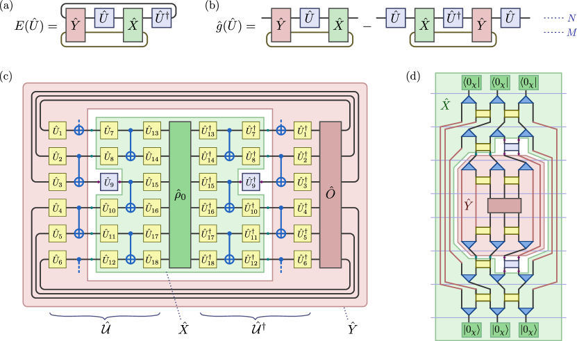
Figure 1: Diagrammatic representations for (a) cost function $E(\hat{U})$ and (b) Riemannian gradient $\hat{g}(\hat{U})$, where we consider the dependence on a single gate $\hat{U}\in\operatorname{U}(N)$ from the variable gates $\{\hat{U}_{i}\in\operatorname{U}(N_{i})\}$ that compose the quantum circuit $\hat{\mathcal{U}}$; cf. Eqs. (3) and (4). Cost functions of this form arise in various applications like quantum machine learning and variational quantum algorithms for the investigation of many-body ground states. Panel (c) shows how a cost function (2) for a quantum circuit consisting of single-qubit and CNOT gates attains the form (3). Panel (d) shows an example for the variational optimization of a multiscale entanglement renormalization ansatz (MERA) Vidal-2005-12 ; Vidal2006 – a hierarchical tensor network state that features unitary disentanglers (yellow squares) and isometries (blue triangles). See Refs. Miao2021_08 ; Miao2023_04 ; Barthel2023_03 for more context.

In this report, we establish a direct connection between cost-function concentration and the decay of Riemannian gradient amplitudes in the optimization of quantum circuits. The proof in the Riemannian formulation is surprisingly simple. We will show that when the gates are sampled according to the uniform Haar measure, the single-gate cost-function variance is exactly half the single-gate variance of the Riemannian gradient. The corresponding total variances, where all gates are varied simultaneously, are both bounded from above by sums of the single-gate variances. Furthermore, the total variances bound all individual single-gate variances. As a consequence, the barren plateau problem can be equivalently diagnosed through the analysis of cost function concentration and cannot be resolved by switching from gradient-based optimization to a gradient-free optimization Arrasmith2022-7 ; Arrasmith2021-5 .

II Cost function and Riemannian gradient

Consider a generic quantum circuit $\hat{\mathcal{U}}$ composed of some fixed unitary gates $\{\hat{W}_{1},\hat{W}_{2},\dotsc\}$ and variable unitary gates $\{\hat{U}_{1},\hat{U}_{2},\dotsc\}$ over which we optimize. Starting from a reference state ${\hat{\rho}}_{0}$, the circuit prepares the state ${\hat{\rho}}=\hat{\mathcal{U}}{\hat{\rho}}_{0}\,\hat{\mathcal{U}}^{\dagger}$. With an observable $\hat{O}$, the cost function takes the form

$$E(\{\hat{U}_{i}\})=\operatorname{Tr}\left(\hat{\mathcal{U}}{\hat{\rho}}_{0}\,\hat{\mathcal{U}}^{\dagger}\hat{O}\right)$$ (2)

With ${\hat{\rho}}_{0}=\sum_{s=1}^{S}{\hat{\rho}}_{s}\otimes|s\rangle\langle s|$ and $\hat{O}=\sum_{s=1}^{S}\hat{O}_{s}\otimes|s\rangle\langle s|$, this setup also covers the more general case $E(\{\hat{U}_{i}\})=\sum_{s=1}^{S}\operatorname{Tr}\left(\hat{\mathcal{U}}{\hat{\rho}}_{s}\,\hat{\mathcal{U}}^{\dagger}\hat{O}_{s}\right)$ with a training set $\{({\hat{\rho}}_{s},\hat{O}_{s})\}$ of $S$ initial states ${\hat{\rho}}_{s}$ and associated measurement operators $\hat{O}_{s}$ Arrasmith2022-7 .

Considering the dependence on one of the variable gates, $\hat{U}\in\operatorname{U}(N)$, we can write the cost function in the compact form

$$E(\hat{U})=\operatorname{Tr}(\hat{Y}\tilde{U}\hat{X}\tilde{U}^{\dagger})\quad\text{with}\quad\tilde{U}:=\hat{U}\otimes\mathbbm{1}_{M}\quad\text{and}\quad\hat{X},\hat{Y}\in\operatorname{End}(\mathbb{C}^{N}\otimes\mathbb{C}^{M}),$$ (3)

where the Hermitian operator $\hat{X}$ comprises ${\hat{\rho}}_{0}$, $\hat{Y}$ comprises $\hat{O}$ and both comprise further circuit gates except $\hat{U}$. See Fig. 1c for an example. As discussed in Refs. Miao2023_04 ; Barthel2023_03 , expectation values $\langle\Psi|\hat{H}|\Psi\rangle$ of a Hamiltonian $\hat{H}$ with respect to isometric tensor network states (TNS) $|\Psi\rangle=\hat{\mathcal{U}}|0\rangle$ can also be written in the form (3). In this case the TNS are generated from a pure reference state $|0\rangle$ by application of a quantum circuit, and $\hat{U}$ corresponds to one tensor of the TNS. The example of a multiscale entanglement renormalization ansatz (MERA) Vidal-2005-12 ; Vidal2006 is illustrated in Fig. 1d.

Here and in Sec. III, we consider variation of one specific unitary gate $\hat{U}$ such that the Riemannian manifold is just $\operatorname{U}(N)$; this is referred to as a “single-gate” variation. The extension to variation of all gates (“total” variation) on the full manifold (1) will be discussed in Sec. IV. The Riemannian gradient of the cost function (3) at $\hat{U}$ is

$$\hat{g}(\hat{U})=\operatorname{Tr}_{M}(\hat{Y}\tilde{U}\hat{X}-\tilde{U}\hat{X}\tilde{U}^{\dagger}\hat{Y}\tilde{U}),$$ (4)

which can be efficiently measured on quantum computers Miao2021_08 ; Wiersema2023-107 . Here and in the following, $\operatorname{Tr}_{N}$ and $\operatorname{Tr}_{M}$ denote the partial traces over the first and second components of $\mathbb{C}^{N}\otimes\mathbb{C}^{M}$, respectively.

Let us summarize the derivation of Eq. (4): The $N\times N$ unitary gates are embedded in the $2N^{2}$ real Euclidean space $\mathcal{E}=\operatorname{End}(\mathbb{C}^{N})\simeq\mathbb{R}^{2N^{2}}$. The gradient in this embedding space is $\hat{d}=\partial_{\hat{U}}E(\hat{U})=2\operatorname{Tr}_{M}(\hat{Y}\tilde{U}\hat{X})$. Using the (Euclidean) metric $(\hat{U},\hat{U}^{\prime}):=\operatorname{Re}\operatorname{Tr}(\hat{U}^{\dagger}\hat{U}^{\prime})$ for the embedding space $\mathcal{E}$, $\hat{d}$ fulfills $\partial_{\varepsilon}E(\hat{U}+\varepsilon\hat{V})|_{\varepsilon=0}=(\hat{d},\hat{V})$ for all $\hat{V}$. For Riemannian optimization algorithms, one needs to project $\hat{d}$ onto the tangent space $\mathcal{T}_{\hat{U}}$ of $\operatorname{U}(N)$ at $\hat{U}$, and then construct retractions for line search, and vector transport to form linear combinations of gradient vectors from different points on the manifold Smith1994-3 ; Huang2015-25 ; Miao2021_08 . An element $\hat{V}$ of the tangent space $\mathcal{T}_{\hat{U}}$ needs to obey $(\hat{U}+\varepsilon\hat{V})^{\dagger}(\hat{U}+\varepsilon\hat{V})=\mathbbm{1}+\mathcal{O}(\varepsilon^{2})$ such that

$$\mathcal{T}_{\hat{U}}=\{\mathrm{i}\mkern 1.0mu\hat{U}\hat{\eta}\,|\,\hat{\eta}=\hat{\eta}^{\dagger}\in\operatorname{End}(\mathbb{C}^{N})\}.$$ (5)

The projection $\hat{g}$ of $\hat{d}$ onto this tangent space obeys $(\hat{V},\hat{g})=(\hat{V},\hat{d})$ for all $\hat{V}\in\mathcal{T}_{\hat{U}}$. This gives the Riemannian gradient $\hat{g}=(\hat{d}-\hat{U}\hat{d}^{\dagger}\hat{U})/2$ which results in Eq. (4).

III Single-gate Haar-measure variances

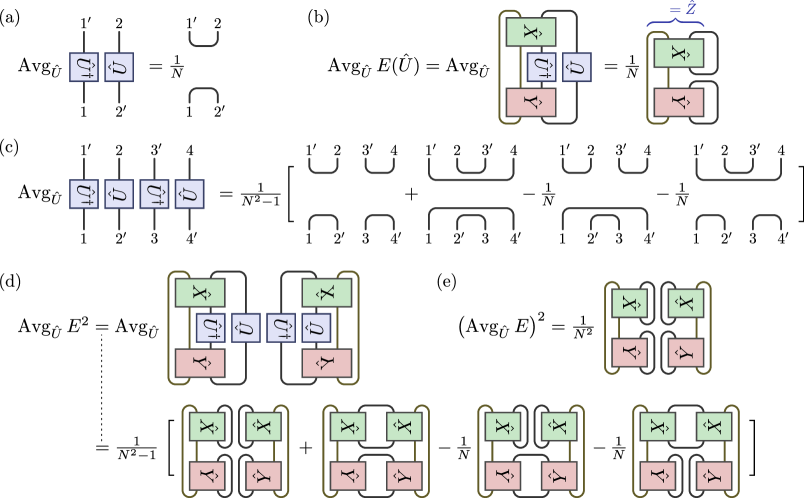
Figure 2: (a) Diagrammatic representation for the first-moment Haar-measure integral (7a) over the unitary group $\operatorname{U}(N)$. (b) The single-gate Haar average (8) of the cost function (3). (c) Second-moment Haar-measure integral (7b) over the unitary group $\operatorname{U}(N)$. (d) Average (10) of the squared cost function. (e) The single-gate Haar variance (11) is obtained by subtracting the squared cost-function average.

To evaluate averages and variances over $\operatorname{U}(N)$ (or, more generally the manifold $\mathcal{M}$), we employ Haar-measure integrals. The average of the Riemannian gradient (4) is zero,

$$\operatorname{Avg}_{\hat{U}}\hat{g}:=\int_{\operatorname{U}(N)}\mathrm{d}U\,\hat{g}(\hat{U})=\frac{1}{2}\int_{\operatorname{U}(N)}\mathrm{d}U\,[\hat{g}(\hat{U})+\hat{g}(-\hat{U})]=0,$$ (6)

because $\hat{g}$ is an odd function in $\hat{U}$. For the evaluation of $\operatorname{Avg}_{\hat{U}}E$ and the variances, we only need the first and second-moment Haar-measure integrals over the unitary group. From the Weingarten formulas Weingarten1978-19 ; Collins2006-264 , one obtains Barthel2023_03

$$\textstyle\operatorname{Avg}_{\hat{U}}\hat{U}^{\dagger}\otimes\hat{U}=\frac{1}{N}\operatorname{Swap}\quad\text{and}$$ (7a)

$$\textstyle\operatorname{Avg}_{\hat{U}}\hat{U}^{\dagger}\otimes\hat{U}\otimes\hat{U}^{\dagger}\otimes\hat{U}=\frac{1}{N^{2}-1}\left(1-\frac{1}{N}\operatorname{Swap}_{2,4}\right)\left(\operatorname{Swap}_{1,2}\operatorname{Swap}_{3,4}+\operatorname{Swap}_{1,4}\operatorname{Swap}_{2,3}\right)$$ (7b)

with $\operatorname{Swap}=\sum_{i,j=1}^{N}|i,j\rangle\langle j,i|$ and $\operatorname{Swap}_{k,\ell}$ swaps the $k^{\text{th}}$ and $\ell^{\text{th}}$ components of $\mathbb{C}^{N}\otimes\mathbb{C}^{N}\otimes\mathbb{C}^{N}\otimes\mathbb{C}^{N}$. The two equations are illustrated in Fig. 2.

Consequently, the cost-function average is

$$\operatorname{Avg}_{\hat{U}}E\stackrel{{\scriptstyle\eqref{eq:G1}}}{{=}}\frac{1}{N}\operatorname{Tr}\left(\operatorname{Tr}_{N}(\hat{X})\operatorname{Tr}_{N}(\hat{Y})\right)=\frac{1}{N}\operatorname{Tr}\hat{Z}$$ (8)

as illustrated in Fig. 2b, where $\hat{Z}\in\operatorname{End}(\mathbb{C}^{N}\otimes\mathbb{C}^{N})$ with

$$\langle i_{1},i_{2}|\hat{Z}|j_{1},j_{2}\rangle=\sum_{m,m^{\prime}=1}^{M}\langle i_{1},m|\hat{X}|j_{1},m^{\prime}\rangle\langle i_{2},m^{\prime}|\hat{Y}|j_{2},m\rangle.$$ (9)

For the cost-function variance $\operatorname{Var}_{\hat{U}}E=\operatorname{Avg}_{\hat{U}}E^{2}-(\operatorname{Avg}_{\hat{U}}E)^{2}$ over $\operatorname{U}(N)$, we have

$$\operatorname{Avg}_{\hat{U}}E^{2}\stackrel{{\scriptstyle\eqref{eq:G2}}}{{=}}\frac{1}{N^{2}-1}\left((\operatorname{Tr}\hat{Z})^{2}-\frac{\operatorname{Tr}\big{(}(\operatorname{Tr}_{1}\hat{Z})^{2}+(\operatorname{Tr}_{2}\hat{Z})^{2}\big{)}}{N}+\operatorname{Tr}\hat{Z}^{2}\right),$$ (10)

where $\operatorname{Tr}_{1}\hat{Z}$ and $\operatorname{Tr}_{2}\hat{Z}$ denote the partial traces of $\hat{Z}$ over the first and second components of $\mathbb{C}^{N}\otimes\mathbb{C}^{N}$, respectively. See Fig. 2d. Hence,

$$\operatorname{Var}_{\hat{U}}E\stackrel{{\scriptstyle\eqref{eq:Eavg},\eqref{eq:E2avg}}}{{=}}\frac{1}{N^{2}-1}\left(\frac{(\operatorname{Tr}\hat{Z})^{2}}{N^{2}}-\frac{\operatorname{Tr}\big{(}(\operatorname{Tr}_{1}\hat{Z})^{2}+(\operatorname{Tr}_{2}\hat{Z})^{2}\big{)}}{N}+\operatorname{Tr}\hat{Z}^{2}\right).$$ (11)

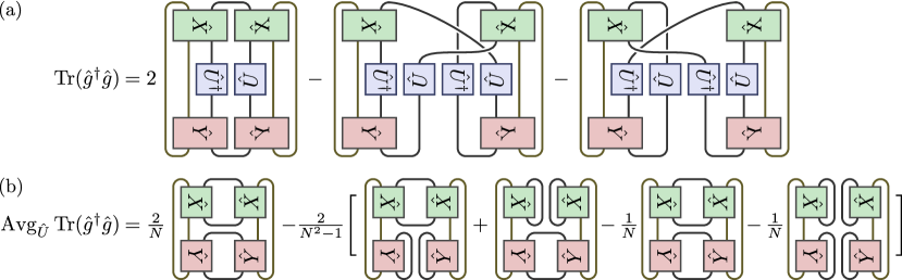
Figure 3: (a) Diagrammatic representation of the central quantity $\operatorname{Tr}(\hat{g}^{\dagger}\hat{g})$ in the definition (12) of the Riemannian gradient variance. (b) The single-gate variance (13) of the Riemannian gradient, obtained by applying the second-moment Weingarten formula (7b) as illustrated in Fig. 2c.

With the average gradient being zero [Eq. (6)], we can quantify the gradient variance by

$$\operatorname{Var}_{\hat{U}}\hat{g}:=\operatorname{Avg}_{\hat{U}}\frac{1}{N}\operatorname{Tr}(\hat{g}^{\dagger}\hat{g}).$$ (12)

As discussed in Ref. Barthel2023_03 and shown diagrammatically in Fig. 3, it evaluates to

$$\operatorname{Var}_{\hat{U}}\hat{g}\stackrel{{\scriptstyle\eqref{eq:Riem_grad},\eqref{eq:G}}}{{=}}\frac{2}{N^{2}-1}\left(\frac{(\operatorname{Tr}\hat{Z})^{2}}{N^{2}}-\frac{\operatorname{Tr}\big{(}(\operatorname{Tr}_{1}\hat{Z})^{2}+(\operatorname{Tr}_{2}\hat{Z})^{2}\big{)}}{N}+\operatorname{Tr}\hat{Z}^{2}\right)$$ (13)

So, the cost-function variance (11) is exactly half of the Riemannian gradient variance (13).

The definition (12) can be motivated as follows Barthel2023_03 : As any element of the tangent space (5), the gradient $\hat{g}$ can be expanded in an orthonormal basis of involutory Hermitian operators $\{\hat{\sigma}_{k}\,|\,\hat{\sigma}_{k}=\hat{\sigma}^{\dagger}_{k}=\hat{\sigma}^{-1}_{k}\}$ for $\operatorname{End}(\mathbb{C}^{N})$ with $\operatorname{Tr}(\hat{\sigma}_{k}\hat{\sigma}_{k^{\prime}})=N\delta_{k,k^{\prime}}$. This gives the gradient in the form $\hat{g}=\mathrm{i}\mkern 1.0mu\hat{U}\sum_{k=1}^{N^{2}}\alpha_{k}\hat{\sigma}_{k}/N$, where each $\alpha_{k}$ corresponds to the derivative of one rotation angle. Hence, $\operatorname{Tr}(\hat{g}^{\dagger}\hat{g})/N=\sum_{k}\alpha_{k}^{2}/N^{2}$, i.e., Eq. (12) is the average variance of the rotation-angle derivatives .

Equations (11) and (13) give the central result of this section.

Theorem 1 (Exact equivalence of single-gate cost-function and gradient variances).

In the Riemannian formulation, the variance of the cost function (2) is exactly half the variance of the Riemannian gradient (4) when considering the dependence on one of the unitary gates of the quantum circuit ($\hat{U}_{j\neq i}$ fixed), i.e.,

$$\operatorname{Var}_{\hat{U}_{i}}E(\{\hat{U}_{j}\})=\frac{1}{2}\operatorname{Var}_{\hat{U}_{i}}\hat{g}_{i}(\{\hat{U}_{j}\})\qquad\forall\ \{\hat{U}_{j\neq i}\}.$$ (14)

Of course, the proportionality of these conditional single-gate variances translates directly into a proportionality of the averaged single-gate variances,

$$V_{i}:=\operatorname{Avg}_{\{\hat{U}_{j\neq i}\}}\operatorname{Var}_{\hat{U}_{i}}E(\{\hat{U}_{j}\})=\frac{1}{2}\operatorname{Avg}_{\{\hat{U}_{j\neq i}\}}\operatorname{Var}_{\hat{U}_{i}}\hat{g}_{i}(\{\hat{U}_{j}\}).$$ (15)

IV Total Haar-measure variances

In Sec. III, we only considered the dependence of the cost function (2) on one of the unitary gates ($\hat{U}$) in the circuit as well as the single-gate gradient 4. In this section, we consider the dependence on all variable unitary gates $(\hat{U}_{1},\hat{U}_{2},\dotsc,\hat{U}_{K})\in\mathcal{M}$ with $\hat{U}_{i}\in\operatorname{U}(N_{i})$ and the corresponding total variances like $\operatorname{Var}_{\{\hat{U}_{j}\}}E\equiv\operatorname{Avg}_{\{\hat{U}_{j}\}}(E^{2})-(\operatorname{Avg}_{\{\hat{U}_{j}\}}E)^{2}$ for the cost function.

For the following, we denote the Riemannian gradient (4) of the cost function with respect to gate $\hat{U}_{i}$ as

$$\hat{g}_{i}\equiv\hat{g}_{i}(\{\hat{U}_{j}\})=\operatorname{Tr}_{M_{i}}(\hat{Y}_{i}\tilde{U}_{i}\hat{X}_{i}-\tilde{U}_{i}\hat{X}_{i}\tilde{U}_{i}^{\dagger}\hat{Y}_{i}\tilde{U}_{i})\quad\text{with}\quad\tilde{U}_{i}:=\hat{U}_{i}\otimes\mathbbm{1}_{M_{i}},$$ (16)

where $\hat{X}_{i}$ and $\hat{Y}_{i}$ depend on the remaining gates of the circuit, ${\hat{\rho}}_{0}$, and $\hat{O}$ as in Eq. (3). The full Riemannian gradient of the cost function (2) with respect to all variable gates is simply the direct sum of the individual gradients, i.e.,

$$\hat{g}_{\text{full}}=\hat{g}_{1}\oplus\hat{g}_{2}\oplus\dotsb\oplus\hat{g}_{K}.$$ (17)

In extension of Eq. (12), we define the total variance of $\hat{g}_{\text{full}}$ as

$$\operatorname{Var}_{\{\hat{U}_{j}\}}\hat{g}_{\text{full}}:=\frac{1}{K}\sum_{i=1}^{K}\operatorname{Avg}_{\{\hat{U}_{j}\}}\frac{1}{N_{i}}\operatorname{Tr}(\hat{g}_{i}^{\dagger}\hat{g}_{i}^{\phantom{{\dagger}}})\stackrel{{\scriptstyle\eqref{eq:gVarDef}}}{{=}}\frac{1}{K}\sum_{i=1}^{K}\operatorname{Avg}_{\{\hat{U}_{j\neq i}\}}\operatorname{Var}_{\hat{U}_{i}}\hat{g}_{i}.$$ (18)

Theorem 2 (Equivalence of circuit cost-function concentration and gradient vanishing).

When averaging over the variable unitaries $\{\hat{U}_{i}\}$ of the quantum circuit $\hat{\mathcal{U}}$ according to the Haar measure, the total variance of the cost function (2) and the total variance of the full Riemannian gradient (18) are both bounded from below by single-gate variances $V_{i}$ [Eqs. (15) and (LABEL:eq:gVarTot)], and they are bounded from above by or proportional to the sum $\sum_{i}V_{i}$,

$$V_{j} \leq \operatorname{Var}_{\hat{U}_{1},\dotsc,\hat{U}_{K}} E(\hat{U}_{1},\dotsc,\hat{U}_{K}) \leq\sum_{i=1}^{K}V_{i}\quad \forall\ j\quad\text{and}$$ (19a)

$$V_{j} \stackrel{{\scriptstyle\eqref{eq:gVarFullDef}}}{{\leq}} \frac{K}{2}\operatorname{Var}_{\hat{U}_{1},\dotsc,\hat{U}_{K}} \hat{g}_{\text{full}}(\hat{U}_{1},\dotsc,\hat{U}_{K}) \stackrel{{\scriptstyle\eqref{eq:gVarFullDef}}}{{=}}\sum_{i=1}^{K}V_{i}\quad \forall\ j.$$ (19b)

In particular, if all single-gate variances $V_{i}$ of polynomial-depth circuits ($K=\operatorname{poly}n$) decay exponentially in the system size (number of qudits) $n$, then both total variances (19) decay exponentially in $n$. Conversely, if one of the total variances decays exponentially in $n$, then all single-gate variances also decay exponentially. So, the barren-plateau problem and exponential cost-function concentration always appear simultaneously.

Proof.

(a) Let us first consider a circuit with only two variable unitaries $\hat{U}_{1}$ and $\hat{U}_{2}$. In this case, the cost function (2) can be written in the form

$$E=E(\hat{U}_{1},\hat{U}_{2})=\sum_{a}f_{a}(\hat{U}_{1})g_{a}(\hat{U}_{2}),$$ (20)

where $f_{a}$ and $g_{a}$ are continuous functions which only depend on $\hat{U}_{1}$ and $\hat{U}_{2}$, respectively: Analogously to Fig. 1c, we can always bipartition the the tensor network for $E(\hat{U}_{1},\hat{U}_{2})$ into two parts $f$ and $g$ with $f$ containing $\hat{U}_{1}^{\phantom{{\dagger}}},\hat{U}_{1}^{\dagger}$ and $g$ containing $\hat{U}_{2}^{\phantom{{\dagger}}},\hat{U}_{2}^{\dagger}$. The contraction of the two parts (operator products and trace to obtain the scalar $E$) then corresponds to the sum over $a$ in Eq. (20).

The single-gate cost variance for $\hat{U}_{1}$ at fixed $\hat{U}_{2}$ then is ($\operatorname{Avg}_{i}\equiv\operatorname{Avg}_{\hat{U}_{i}}$ and $\operatorname{Var}_{i}\equiv\operatorname{Var}_{\hat{U}_{i}}$)

$$\operatorname{Var}_{1}E(\hat{U}_{1},\hat{U}_{2}) =\operatorname{Avg}_{1}(E^{2})-(\operatorname{Avg}_{1}E)^{2}$$

$$=\sum_{a,b}\underbrace{\left[\operatorname{Avg}_{1}(f_{a}f_{b})-\operatorname{Avg}_{1}(f_{a})\operatorname{Avg}_{1}(f_{b})\right]}_{\equiv\operatorname{Cov}(f_{a},f_{b})}g_{a}g_{b}$$ (21)

and, similarly $\operatorname{Var}_{2}E=\sum_{a,b}f_{a}f_{b}\operatorname{Cov}(g_{a},g_{b})$.

Using that $\operatorname{Avg}_{1,2}(f_{a}f_{b}g_{a}g_{b})=\operatorname{Avg}_{1}(f_{a}f_{b})\operatorname{Avg}_{2}(g_{a}g_{b})$ due to the independence of $\hat{U}_{1}$ and $\hat{U}_{2}$ in the Haar-measure average, the global cost-function variance is ($\operatorname{Avg}_{1,2}\equiv\operatorname{Avg}_{\hat{U}_{1},\hat{U}_{2}}\equiv\operatorname{Avg}_{\hat{U}_{1}}\operatorname{Avg}_{\hat{U}_{2}}$)

$$\operatorname{Var}_{1,2}E =\operatorname{Avg}_{1,2}(E^{2})-(\operatorname{Avg}_{1,2}E)^{2}$$

$$=\sum_{a,b}\left[\operatorname{Avg}_{1}(f_{a}f_{b})\operatorname{Avg}_{2}(g_{a}g_{b})-\operatorname{Avg}_{1}(f_{a})\operatorname{Avg}_{1}(f_{b})\operatorname{Avg}_{2}(g_{a})\operatorname{Avg}_{2}(g_{b})\right]$$

$$=\operatorname{Avg}_{2}\operatorname{Var}_{1}E+\operatorname{Avg}_{1}\operatorname{Var}_{2}E-\sum_{a,b}\operatorname{Cov}(f_{a},f_{b})\operatorname{Cov}(g_{a},g_{b})$$

$$\leq\operatorname{Avg}_{2}\operatorname{Var}_{1}E+\operatorname{Avg}_{1}\operatorname{Var}_{2}E$$ (22)

This is the right inequality in Eq. (19a) for the case of two variable unitaries. In the last step, we have used that the covariance matrices

$$\operatorname{Cov}(f_{a},f_{b})=\operatorname{Avg}(f_{a}f_{b})-\operatorname{Avg}(f_{a})\operatorname{Avg}(f_{b})=\operatorname{Avg}\left([f_{a}-\operatorname{Avg}f_{a}][f_{b}-\operatorname{Avg}f_{b}]\right)$$ (23)

and $\operatorname{Cov}(g_{a},g_{b})$ are positive semidefinite such that the trace $\sum_{a,b}\operatorname{Cov}(f_{a},f_{b})\operatorname{Cov}(g_{a},g_{b})$ of their product is non-negative.

(b) The generalization to a circuit with $K$ variable unitaries follows by iterating Eq. (22). Decomposing the tensor network as before into $K$ parts, each containing only one of the variable unitaries and its adjoint, we can write the cost function in the form

$$E=E(\hat{U}_{1},\hat{U}_{2},\dotsc,\hat{U}_{K})=\sum_{a}f^{(1)}_{a}(\hat{U}_{1})f^{(2)}_{a}(\hat{U}_{2})\dotsb f^{(K)}_{a}(\hat{U}_{K}).$$ (24)

Now, iterating Eq. (22), we find

$$\operatorname{Var}_{1,2,\dotsc,K}E \leq\operatorname{Avg}_{2,\dotsc,K}\operatorname{Var}_{1}E+\operatorname{Avg}_{1}\operatorname{Var}_{2,\dotsc,K}E$$

$$\leq\operatorname{Avg}_{2,\dotsc,K}\operatorname{Var}_{1}E+\operatorname{Avg}_{1}\left(\operatorname{Avg}_{3,\dotsc,K}\operatorname{Var}_{2}E+\operatorname{Avg}_{2}\operatorname{Var}_{3,\dotsc,K}E\right)$$

$$\leq\dots\leq\sum_{i}\operatorname{Avg}_{\{j\neq i\}}\operatorname{Var}_{i}E\equiv\sum_{i}V_{i},$$

where $\operatorname{Avg}_{i_{1},\dotsc,i_{n}}h\equiv\operatorname{Avg}_{i_{1}}\dots\operatorname{Avg}_{i_{n}}h$ and $\operatorname{Var}_{i_{1},\dots,i_{n}}h\equiv\operatorname{Avg}_{i_{1},\dotsc,i_{n}}h^{2}-(\operatorname{Avg}_{i_{1},\dotsc,i_{n}}h)^{2}$.

(c) The right inequality in Eq. (19a) follows by applying the law of total variance,

$$\operatorname{Var}_{1,2,\dotsc,K}E=\operatorname{Avg}_{\{j\neq i\}}\operatorname{Var}_{i}E+\operatorname{Var}_{\{j\neq i\}}\operatorname{Avg}_{i}E\geq\operatorname{Avg}_{\{j\neq i\}}\operatorname{Var}_{i}E\stackrel{{\scriptstyle\eqref{eq:singleGateVar}}}{{\equiv}}V_{i},$$ (25)

which holds for all $i$. ∎

Note that the conclusions below Eq. (19b) remain valid if we choose a different weighting in the definition of the full gradient variance (18). For example, we could also define it as $\frac{1}{\sum_{i=1}^{K}N_{i}^{2}}\sum_{i=1}^{K}N_{i}\operatorname{Avg}_{\{\hat{U}_{j}\}}\operatorname{Tr}(\hat{g}_{i}^{\dagger}\hat{g}_{i}^{\phantom{{\dagger}}})$, corresponding to an equal weighting of all rotation-angle derivatives in the parametrization discussed below Eq. (13).

V Discussion

Given the equivalence of cost-function concentration and gradient vanishing on both the single-gate as well as circuit levels (Theorems 1 and 2, respectively), we can assess gradient vanishing and, especially, barren plateaus more easily through the scalar cost function. In fact, this route has already been pursued in recent analytic works on the trainability of variational quantum algorithms Thanasilp2022_08 ; Rudolph2023_05 ; Ragone2023_09 ; Diaz2023_10 ; Cerezo2023_12 ; Xiong2023_12 .

Inspired by the work of Arrasmith et al. Arrasmith2022-7 on the parametrized circuits and Euclidean gradients, we studied the question in the Riemannian formulation which makes the proofs rather simple and yields additional insights: (a) The single-gate variances of gradients and of the cost function turn out to be strictly proportional. (b) In the Euclidean formulation, Arrasmith et al. obtained results for the variance of cost-function differences like $\operatorname{Var}_{{\bm{\theta}}}\left(E({\bm{\theta}}^{\prime})-E({\bm{\theta}})\right)\leq K^{2}V(n)$, where ${\bm{\theta}}^{\prime}$ is another random reference point and $V(n)$ is a common upper bound for all $V_{i}(n)$ as a function of the system size $n$. This difference construction turned out to be unnecessary in the Riemannian formulation and we could access $\operatorname{Var}_{\hat{U}_{1},\dotsc,\hat{U}_{K}}E$ directly. (c) Furthermore, we obtained the tighter bound $\operatorname{Var}_{\hat{U}_{1},\dotsc,\hat{U}_{K}}E\leq KV(n)$. This result aligns with our experience in numerical simulations and could probably be further tightened.

- (1) M. Cerezo, A. Arrasmith, R. Babbush, S. C. Benjamin, S. Endo, K. Fujii, J. R. McClean, K. Mitarai, X. Yuan, L. Cincio, and P. J. Coles, Variational quantum algorithms, Nat. Rev. Phys. 3, 625 (2021).
- (2) J. R. McClean, S. Boixo, V. N. Smelyanskiy, R. Babbush, and H. Neven, Barren plateaus in quantum neural network training landscapes, Nat. Commun. 9, 4812 (2018).
- (3) M. Cerezo, A. Sone, T. Volkoff, L. Cincio, and P. J. Coles, Cost function dependent barren plateaus in shallow parametrized quantum circuits, Nat. Commun. 12, 1791 (2021).
- (4) E. Grant, L. Wossnig, M. Ostaszewski, and M. Benedetti, An initialization strategy for addressing barren plateaus in parametrized quantum circuits, Quantum 3, 214 (2019).
- (5) K. Zhang, M.-H. Hsieh, L. Liu, and D. Tao, Gaussian initializations help deep variational quantum circuits escape from the barren plateau, arXiv:2203.09376 (2022).
- (6) A. A. Mele, G. B. Mbeng, G. E. Santoro, M. Collura, and P. Torta, Avoiding barren plateaus via transferability of smooth solutions in Hamiltonian Variational Ansatz, arXiv:2206.01982 (2022).
- (7) A. Kulshrestha and I. Safro, BEINIT: Avoiding barren plateaus in variational quantum algorithms, arXiv:2204.13751 (2022).
- (8) J. Dborin, F. Barratt, V. Wimalaweera, L. Wright, and A. G. Green, Matrix product state pre-training for quantum machine learning, Quant. Sci. Tech. 7, 035014 (2022).
- (9) A. Skolik, J. R. McClean, M. Mohseni, P. van der Smagt, and M. Leib, Layerwise learning for quantum neural networks, Quantum Mach. Intell. 3, 5 (2021).
- (10) L. Slattery, B. Villalonga, and B. K. Clark, Unitary block optimization for variational quantum algorithms, Phys. Rev. Research 4, 023072 (2022).
- (11) T. Haug and M. Kim, Optimal training of variational quantum algorithms without barren plateaus, arXiv:2104.14543 (2021).
- (12) S. H. Sack, R. A. Medina, A. A. Michailidis, R. Kueng, and M. Serbyn, Avoiding barren plateaus using classical shadows, PRX Quantum 3, 020365 (2022).
- (13) A. Rad, A. Seif, and N. M. Linke, Surviving the barren plateau in variational quantum circuits with Bayesian learning initialization, arXiv:2203.02464 (2022).
- (14) Z. Tao, J. Wu, Q. Xia, and Q. Li, LAWS: Look around and warm-start natural gradient descent for quantum neural networks, arXiv:2205.02666 (2022).
- (15) Y. Wang, B. Qi, C. Ferrie, and D. Dong, Trainability enhancement of parameterized quantum circuits via reduced-domain parameter initialization, arXiv:2302.06858 (2023).
- (16) Q. Miao and T. Barthel, Isometric tensor network optimization for extensive Hamiltonians is free of barren plateaus, arXiv:2304.14320 (2023).
- (17) T. Barthel and Q. Miao, Absence of barren plateaus and scaling of gradients in the energy optimization of isometric tensor network states, arXiv:2304.00161 (2023).
- (18) A. Arrasmith, Z. Holmes, M. Cerezo, and P. J. Coles, Equivalence of quantum barren plateaus to cost concentration and narrow gorges, Quantum Sci. Technol. 7, 045015 (2022).
- (19) S. T. Smith, in Hamiltonian and Gradient Flows, Algorithms, and Control, Vol. 3 of Fields Institute Communications (AMS, Providence, RI, 1994), Chap. Optimization techniques on Riemannian manifolds, p. 113.
- (20) W. Huang, K. A. Gallivan, and P.-A. Absil, A Broyden class of quasi-Newton methods for Riemannian optimization, SIAM Journal on Optimization 25, 1660 (2015).
- (21) Q. Miao and T. Barthel, Quantum-classical eigensolver using multiscale entanglement renormalization, Phys. Rev. Research 5, 033141 (2023).
- (22) R. Wiersema and N. Killoran, Optimizing quantum circuits with Riemannian gradient flow, Phys. Rev. A 107, 062421 (2023).
- (23) G. Vidal, Entanglement renormalization, Phys. Rev. Lett. 99, 220405 (2007).
- (24) G. Vidal, Class of quantum many-body states that can be efficiently simulated, Phys. Rev. Lett. 101, 110501 (2008).
- (25) A. Arrasmith, M. Cerezo, P. Czarnik, L. Cincio, and P. J. Coles, Effect of barren plateaus on gradient-free optimization, Quantum 5, 558 (2021).
- (26) D. Weingarten, Asymptotic behavior of group integrals in the limit of infinite rank, J. Math. Phys. 19, 999 (1978).
- (27) B. Collins and P. Śniady, Integration with respect to the Haar measure on unitary, orthogonal and symplectic group, Commun. in Math. Phys. 264, 773 (2006).
- (28) We ignore the heterogeneity of for different of a single gate, because the gate Hilbert-space dimension is usually system-size independent.
- (29) S. Thanasilp, S. Wang, M. Cerezo, and Z. Holmes, Exponential concentration and untrainability in quantum kernel methods, arXiv:2208.11060 (2022).
- (30) M. S. Rudolph, S. Lerch, S. Thanasilp, O. Kiss, S. Vallecorsa, M. Grossi, and Z. Holmes, Trainability barriers and opportunities in quantum generative modeling, arXiv:2305.02881 (2023).
- (31) M. Ragone, B. N. Bakalov, F. Sauvage, A. F. Kemper, C. O. Marrero, M. Larocca, and M. Cerezo, A unified theory of barren plateaus for deep parametrized quantum circuits, arXiv:2309.09342 (2023).
- (32) N. L. Diaz, D. García-Martín, S. Kazi, M. Larocca, and M. Cerezo, Showcasing a barren plateau theory beyond the dynamical Lie algebra, arXiv:2310.11505 (2023).
- (33) M. Cerezo, M. Larocca, D. García-Martín, N. L. Diaz, P. Braccia, E. Fontana, M. S. Rudolph, P. Bermejo, A. Ijaz, S. Thanasilp, E. R. Anschuetz, and Z. Holmes, Does provable absence of barren plateaus imply classical simulability? Or, why we need to rethink variational quantum computing, arXiv:2312.09121 (2023).
- (34) W. Xiong, G. Facelli, M. Sahebi, O. Agnel, T. Chotibut, S. Thanasilp, and Z. Holmes, On fundamental aspects of quantum extreme learning machines, arXiv:2312.15124 (2023).