Implicit Bias of Policy Gradient in Linear Quadratic Control:
Extrapolation to Unseen Initial States

Abstract

In modern machine learning, models can often fit training data in numerous ways, some of which perform well on unseen (test) data, while others do not. Remarkably, in such cases gradient descent frequently exhibits an implicit bias that leads to excellent performance on unseen data. This implicit bias was extensively studied in supervised learning, but is far less understood in optimal control (reinforcement learning). There, learning a controller applied to a system via gradient descent is known as policy gradient, and a question of prime importance is the extent to which a learned controller extrapolates to unseen initial states. This paper theoretically studies the implicit bias of policy gradient in terms of extrapolation to unseen initial states. Focusing on the fundamental Linear Quadratic Regulator (LQR) problem, we establish that the extent of extrapolation depends on the degree of exploration induced by the system when commencing from initial states included in training. Experiments corroborate our theory, and demonstrate its conclusions on problems beyond LQR, where systems are non-linear and controllers are neural networks. We hypothesize that real-world optimal control may be greatly improved by developing methods for informed selection of initial states to train on.

1 Introduction

The ability to generalize from training data to unseen test data is a core aspect of machine learning. Broadly speaking, there are two types of generalization one may hope for: (i) in-distribution generalization, where test data is drawn from the same distribution as training data; and (ii) out-of-distribution generalization, also known as extrapolation, where test data is drawn from a different distribution than that of the training data. In modern regimes the training objective is often underdetermined — i.e. it admits multiple solutions (parameter assignments fitting training data) that differ in their performance on test data — and the extent to which a learned solution generalizes is determined by an implicit bias of the training algorithm (Neyshabur, 2017; Vardi, 2023). Remarkably, variants of gradient descent frequently converge to solutions with excellent in-distribution generalization (see Zhang et al. (2017)), which in some cases extends to out-of-distribution generalization (cf. Miller et al. (2021)). The implicit bias of gradient descent has accordingly attracted vast theoretical interest, with existing analyses focusing primarily on the basic framework of supervised learning (see, e.g., Neyshabur et al. (2014); Gunasekar et al. (2017); Soudry et al. (2018); Arora et al. (2019); Ji & Telgarsky (2019a, b); Woodworth et al. (2020); Razin & Cohen (2020); Lyu & Li (2020); Lyu et al. (2021); Pesme et al. (2021); Razin et al. (2021, 2022); Frei et al. (2023b, a); Abbe et al. (2023)).

As opposed to supervised learning, little is known about the implicit bias of gradient descent in the challenging framework of optimal control (see overview of related work in Section 2). In optimal control — which in its broadest form is equivalent to reinforcement learning — the goal is to learn a controller (also known as policy) that will steer a given system (also known as environment) such that a given cost is minimized (or equivalently, a given reward is maximized) (Sontag, 2013). Algorithms that learn a controller by directly parameterizing it and setting its parameters through gradient descent are known as policy gradient methods. For implementing such methods, gradients with respect to controller parameters are either estimated via sampling (Williams, 1992), or, in cases where differentiable forms for the system and cost are at hand, the gradients may be computed through analytic differentiation (see, e.g., Hu et al. (2019); Qiao et al. (2020); Clavera et al. (2020); Mora et al. (2021); Gillen & Byl (2022); Howell et al. (2022); Xu et al. (2022); Wiedemann et al. (2023)).

An issue of prime importance in optimal control (and reinforcement learning) is the extent to which a learned controller extrapolates to initial states unseen in training. Indeed, in real-world settings training is often limited to few initial states, and a deployed controller is likely to encounter initial states that go well beyond what it has seen in training (Zhu et al., 2020; Dulac-Arnold et al., 2021). The ability of the controller to handle such initial states is imperative, particularly in safety-critical applications (e.g. robotics, industrial manufacturing, or autonomous driving).

The current paper seeks to take first steps towards theoretically addressing the following question.

To what extent does the implicit bias of policy gradient lead to extrapolation to initial states unseen in training?

As a testbed for theoretical study, we consider the fundamental Linear Quadratic Regulator (LQR) problem (Anderson & Moore, 2007). There, systems are linear, costs are quadratic, and it is known that optimal controllers are linear (Anderson & Moore, 2007). Learning linear controllers in LQR via policy gradient has been the subject of various theoretical analyses (e.g., Fazel et al. (2018); Malik et al. (2019); Bhandari & Russo (2019); Mohammadi et al. (2019, 2021); Bu et al. (2019, 2020); Jin et al. (2020); Gravell et al. (2020); Hambly et al. (2021); Hu et al. (2023)). However, these analyses do not treat underdetermined training objectives, thus leave open our question on the effect of implicit bias on extrapolation. To facilitate its study, we focus on LQR training objectives that are underdetermined.

Our theoretical analysis reveals that in underdetermined LQR problems, the extent to which linear controllers learned via policy gradient extrapolate to initial states unseen in training, depends on the interplay between the system and the initial states that were seen in training. In particular, it depends on the degree of exploration induced by the system when commencing from initial states seen in training. We prove that if this exploration is insufficient, extrapolation does not take place. On the other hand, we construct a setting that encourages exploration, and show that under it extrapolation can be perfect. We then consider a typical setting, i.e. one in which systems are generated randomly and initial states seen in training are arbitrary. In this setting, we prove that the degree of exploration suffices for there to be non-trivial extrapolation — in expectation, and with high probability if the state space dimension is sufficiently large.

Two attributes of our analysis may be of independent interest. First, are advanced tools we employ from the intersection of random matrix theory and topology. Second, is a result by which the implicit bias of policy gradient over a linear controller does not minimize the Euclidean norm, in stark contrast to the implicit bias of gradient descent over linear predictors in supervised learning (cf. Zhang et al. (2017)).

We corroborate our theory through experiments, demonstrating that the interplay between a linear system and initial states seen in training can lead a linear controller (learned via policy gradient) to extrapolate to initial states unseen in training. Moreover, we show empirically that the phenomenon extends to non-linear systems and (non-linear) neural network controllers.

In real-world optimal control (and reinforcement learning), contemporary learning algorithms often extrapolate poorly to initial states unseen in training (Rajeswaran et al., 2017; Zhang et al., 2018, 2019; Fujimoto et al., 2019; Witty et al., 2021). Our results lead us to believe that this extrapolation may be greatly improved by developing methods for informed selection of initial states to train on. We hope that our work will encourage research along this line.

Paper organization. The remainder of the paper is organized as follows. Section 2 reviews related work. Section 3 establishes preliminaries. Section 4 delivers our theoretical analysis — a characterization of extrapolation to unseen initial states for linear controllers trained via policy gradient in underdetermined LQR problems. Section 5 presents experiments with the analyzed LQR problems, as well as with non-linear systems and (non-linear) neural network controllers. Lastly, Section 6 concludes.

2 Related Work

Most theoretical analyses of the implicit bias of gradient descent (or variants thereof) focus on the basic framework of supervised learning. Such analyses traditionally aim to establish in-distribution generalization, or to characterize solutions found in training without explicit reference to test data (see, e.g., Neyshabur et al. (2014); Gunasekar et al. (2017); Soudry et al. (2018); Arora et al. (2019); Ji & Telgarsky (2019a, b); Woodworth et al. (2020); Razin & Cohen (2020); Lyu & Li (2020); Lyu et al. (2021); Azulay et al. (2021); Pesme et al. (2021); Razin et al. (2021, 2022); Andriushchenko et al. (2023); Frei et al. (2023b, a); Marcotte et al. (2023); Chou et al. (2023, 2024)). Among recent analyses are also ones centering on out-of-distribution generalization, i.e. on extrapolation (see Xu et al. (2021); Abbe et al. (2022, 2023); Cohen-Karlik et al. (2022, 2023); Zhou et al. (2023)). These are motivated by the fact that in many real-world scenarios, training and test data are drawn from different distributions (Shen et al., 2021). Our work is similar in that it also centers on extrapolation, and is also motivated by real-world scenarios (see Section 1). It differs in that it studies the challenging framework of optimal control.

In optimal control, theoretical analyses of the implicit bias of gradient descent are relatively scarce. For reinforcement learning, which in a broad sense is equivalent to optimal control: Hu et al. (2021) characterized a tendency towards high-entropy solutions with softmax parameterized policies; and Kumar et al. (2021, 2022) revealed detrimental effects of implicit bias with value-based methods. More relevant to our work are Zhang et al. (2020, 2021); Zhao et al. (2023), which for different LQR problems, establish that policy gradient implicitly enforces certain constraints on the parameters of a controller throughout optimization. These analyses, however, do not treat underdetermined training objectives (they pertain to settings where there is a unique controller minimizing the training objective), thus leave open our question on the effect of implicit bias on extrapolation. To the best of our knowledge, the current paper provides the first analysis of the implicit bias of policy gradient for underdetermined LQR problems. Moreover, for optimal control problems in general, it provides the first analysis of the extent to which the implicit bias of policy gradient leads to extrapolation to initial states unseen in training.

Aside from Zhang et al. (2020, 2021); Zhao et al. (2023), existing theoretical analyses of policy gradient for LQR problems largely fall into two categories. First, are those proving convergence rates to the minimal cost, typically under assumptions ensuring a unique solution (Fazel et al., 2018; Malik et al., 2019; Bhandari & Russo, 2019; Mohammadi et al., 2019, 2021; Bu et al., 2019, 2020; Jin et al., 2020; Gravell et al., 2020; Hambly et al., 2021; Hu et al., 2023). Second, are those establishing sub-linear regret in online learning (Cohen et al., 2018; Agarwal et al., 2019a, b; Cassel & Koren, 2021; Hazan & Singh, 2022; Chen et al., 2023). Both lines of work do not address the topic of implicit bias, which we focus on.

Finally, an empirical observation related to our work is that in real-world optimal control (and reinforcement learning), contemporary learning algorithms often extrapolate poorly to initial states unseen in training (Rajeswaran et al., 2017; Zhang et al., 2018, 2019; Fujimoto et al., 2019; Witty et al., 2021). This observation motivated our work, and our results suggest approaches for alleviating the limitation it reveals (see Section 6).

3 Preliminaries

Notation. We use $\norm{\cdot}$ to denote the Euclidean norm of a vector or matrix, $[N]$ to denote the set $\{1,\ldots,N\}$, where $N\in{\mathbb{N}}$, and $\%$ to denote the modulo operator. We let ${\mathbf{e}}_{1},\ldots,{\mathbf{e}}_{D}\in{\mathbb{R}}^{D}$ be the standard basis vectors. Lastly, the subspace orthogonal to ${\mathcal{X}}\subset{\mathbb{R}}^{D}$ is denoted by ${\mathcal{X}}^{\perp}$, i.e. ${\mathcal{X}}^{\perp}:=\brk[c]{{\mathbf{v}}\in{\mathbb{R}}^{D}:{\mathbf{v}}\perp{\mathbf{x}}~{},~{}\forall{\mathbf{x}}\in{\mathcal{X}}}$.

3.1 Policy Gradient in Linear Quadratic Control

We consider a linear system, in which an initial state ${\mathbf{x}}_{0}\in{\mathbb{R}}^{D}$ evolves according to:

$${\mathbf{x}}_{h}={\mathbf{A}}{\mathbf{x}}_{h-1}+{\mathbf{B}}{\mathbf{u}}_{h-1}~{}~{},~{}\forall h\in{\mathbb{N}}\text{\,,}$$

where ${\mathbf{A}}\in{\mathbb{R}}^{D\times D}$ and ${\mathbf{B}}^{D\times M}$ are matrices that define the system, and ${\mathbf{u}}_{h-1}\in{\mathbb{R}}^{M}$ is the control at time ${h-1}$. An LQR problem of horizon $H\in{\mathbb{N}}$ over this system amounts to searching for controls ${\mathbf{u}}_{0},\ldots,{\mathbf{u}}_{H}$ that minimize the following quadratic cost:

$$\sum\nolimits_{h=0}^{H}{\mathbf{x}}_{h}^{\top}{\mathbf{Q}}{\mathbf{x}}_{h}+{\mathbf{u}}_{h}^{\top}{\mathbf{R}}{\mathbf{u}}_{h}\text{\,,}$$

where ${\mathbf{Q}}\in{\mathbb{R}}^{D\times D}$ and ${\mathbf{R}}\in{\mathbb{R}}^{M\times M}$ are positive semidefinite matrices that define the cost. It is known that for this problem, optimal controls are attained by a (state-feedback) linear controller (Anderson & Moore, 2007), i.e. by setting each control ${\mathbf{u}}_{h}$ to be a certain linear function of the corresponding state ${\mathbf{x}}_{h}$. Accordingly, and in line with prior work (e.g., Fazel et al. (2018); Bu et al. (2019); Malik et al. (2019)), we consider learning a linear controller parameterized by ${\mathbf{K}}\in{\mathbb{R}}^{M\times D}$, which at time $h\in\{0\}\cup[H]$ assigns the control ${\mathbf{u}}_{h}={\mathbf{K}}{\mathbf{x}}_{h}$. The cost attained by ${\mathbf{K}}$ with respect to a finite set ${\mathcal{X}}\subset{\mathbb{R}}^{D}$ of initial states is:

$$J({\mathbf{K}};{\mathcal{X}})\!:=\!\frac{1}{\abs{{\mathcal{X}}}}\!\sum\nolimits_{{\mathbf{x}}_{0}\in{\mathcal{X}}}\sum\nolimits_{h=0}^{H}{\mathbf{x}}_{h}^{\top}{\mathbf{Q}}{\mathbf{x}}_{h}+{\mathbf{x}}_{h}^{\top}{\mathbf{K}}^{\top}{\mathbf{R}}{\mathbf{K}}{\mathbf{x}}_{h}\text{\,,}$$ (1)

where, for each ${\mathbf{x}}_{0}\in{\mathcal{X}}$, the states ${\mathbf{x}}_{1},\ldots,{\mathbf{x}}_{H}$ satisfy:

$${\mathbf{x}}_{h}={\mathbf{A}}{\mathbf{x}}_{h-1}+{\mathbf{B}}{\mathbf{K}}{\mathbf{x}}_{h-1}=({\mathbf{A}}+{\mathbf{B}}{\mathbf{K}})^{h}{\mathbf{x}}_{0}\text{\,.}$$ (2)

Given a (finite) set ${\mathcal{S}}\subset{\mathbb{R}}^{D}$ of initial states seen in training, the controller ${\mathbf{K}}$ is learned by minimizing the training cost $J(\cdot\,;{\mathcal{S}})$. Learning via policy gradient amounts to iteratively updating the controller as follows:

$${\mathbf{K}}^{(t+1)}={\mathbf{K}}^{(t)}-\eta\cdot\nabla J\brk{{\mathbf{K}}^{(t)};{\mathcal{S}}}~{}~{},~{}\forall t\in{\mathbb{N}}\text{\,,}$$ (3)

where $\eta>0$ is a predetermined learning rate, and we assume throughout that ${\mathbf{K}}^{(1)}={\mathbf{0}}$.

3.2 Underdetermined Linear Quadratic Control

Existing analyses of policy gradient for learning linear controllers in LQR (e.g., Fazel et al. (2018); Malik et al. (2019); Bu et al. (2019, 2020); Mohammadi et al. (2019, 2021); Bhandari & Russo (2019); Hambly et al. (2021)) typically assume that ${\mathbf{R}}$ is positive definite, meaning that controls are regularized, and that the set ${\mathcal{S}}$ of initial states seen in training spans ${\mathbb{R}}^{D}$ (or similarly, when training over a distribution of initial states, that the support of the distribution spans ${\mathbb{R}}^{D}$). Under these assumptions, the training cost $J(\cdot\,;{\mathcal{S}})$ is not underdetermined — it entails a single global minimizer, which produces optimal controls from any initial state. Thus, our question on the effect of implicit bias on extrapolation (see Section 1) is not applicable.

To facilitate a study of the foregoing question, we focus on underdetermined problems (ones in which the training cost entails multiple global minimizers), obtained through the following assumptions: (i) ${\mathbf{R}}={\mathbf{0}}$, meaning that controls are unregularized; (ii) $M=D$ and ${\mathbf{B}}\in{\mathbb{R}}^{D\times D}$ has full rank, implying that the controller’s ability to affect the state is not limited; and (iii) the set ${\mathcal{S}}$ of initial states seen in training does not span ${\mathbb{R}}^{D}$ (note that this implies $D\geq 2$). For conciseness, in the main text we fix ${\mathbf{Q}}$ to be an identity matrix, and assume that ${\mathbf{B}}$ is an orthogonal matrix. Extensions of our results to more general ${\mathbf{Q}}$ and ${\mathbf{B}}$ are discussed throughout.

In our setting of interest, the cost attained by a controller ${\mathbf{K}}$ with respect to an arbitrary (finite) set ${\mathcal{X}}\subset{\mathbb{R}}^{D}$ of initial states (Equation 1) simplifies to:

$$J({\mathbf{K}};{\mathcal{X}})=\frac{1}{\abs{{\mathcal{X}}}}\sum\nolimits_{{\mathbf{x}}_{0}\in{\mathcal{X}}}\sum\nolimits_{h=0}^{H}\norm*{({\mathbf{A}}+{\mathbf{B}}{\mathbf{K}})^{h}{\mathbf{x}}_{0}}^{2}\text{,}$$ (4)

with the global minimum of this cost being:

$$J^{*}({\mathcal{X}}):=\min\nolimits_{{\mathbf{K}}\in{\mathbb{R}}^{D\times D}}J({\mathbf{K}};{\mathcal{X}})=\frac{1}{\abs{{\mathcal{X}}}}\sum\nolimits_{{\mathbf{x}}_{0}\in{\mathcal{X}}}\norm{{\mathbf{x}}_{0}}^{2}\text{\,.}$$

A controller ${\mathbf{K}}\in{\mathbb{R}}^{D\times D}$ attains this global minimum if and only if ${\mathbf{K}}{\mathbf{x}}_{0}=-{\mathbf{B}}^{-1}{\mathbf{A}}{\mathbf{x}}_{0}$ for all ${\mathbf{x}}_{0}\in{\mathcal{X}}$, or equivalently:

$$\norm*{({\mathbf{A}}+{\mathbf{B}}{\mathbf{K}}){\mathbf{x}}_{0}}^{2}=0~{}~{},~{}\forall{\mathbf{x}}_{0}\in{\mathcal{X}}\text{\,,}$$ (5)

i.e. every ${\mathbf{x}}_{0}\in{\mathcal{X}}$ is mapped to zero by the state dynamics that ${\mathbf{K}}$ induces.

To see that in our setting the training cost $J(\cdot\,;{\mathcal{S}})$ is indeed underdetermined, notice that, since the set ${\mathcal{S}}$ of initial states seen in training does not span ${\mathbb{R}}^{D}$, there exist infinitely many controllers ${\mathbf{K}}$ satisfying:

$${\mathbf{K}}{\mathbf{x}}_{0}=-{\mathbf{B}}^{-1}{\mathbf{A}}{\mathbf{x}}_{0}~{}~{},~{}\forall{\mathbf{x}}_{0}\in{\mathcal{S}}\text{\,.}$$ (6)

That is, there are infinitely many controllers minimizing the training cost. We denote by ${\mathcal{K}}_{\mathcal{S}}$ the (infinite) set comprising these controllers, i.e.:

$${\mathcal{K}}_{\mathcal{S}}:=\brk[c]*{{\mathbf{K}}\in{\mathbb{R}}^{D\times D}:J({\mathbf{K}};{\mathcal{S}})=J^{*}({\mathcal{S}})}\text{\,.}$$ (7)

3.3 Quantifying Extrapolation

Let ${\mathcal{U}}$ be an (arbitrary) orthonormal basis for ${\mathcal{S}}^{\perp}$ (subspace orthogonal to the initial states seen in training). A controller ${\mathbf{K}}$ is fully determined by the controls it assigns to states in ${\mathcal{S}}$ and ${\mathcal{U}}$. The controllers in ${\mathcal{K}}_{\mathcal{S}}$ (Equation 7), i.e. the controllers minimizing the training cost, all satisfy Equation 6, and in particular agree on the controls they assign to states in ${\mathcal{S}}$. However, they differ arbitrarily in the controls they assign to states in ${\mathcal{U}}$. The performance of a controller ${\mathbf{K}}$ on states in ${\mathcal{U}}$ will quantify extrapolation of ${\mathbf{K}}$ to initial states unseen in training. Two measures will facilitate this quantification. The first, referred to as the optimality measure, is based on the optimality condition in Equation 5. Namely, it measures extrapolation by how close $\norm{({\mathbf{A}}+{\mathbf{B}}{\mathbf{K}}){\mathbf{x}}_{0}}^{2}$ is to zero for every ${\mathbf{x}}_{0}\in{\mathcal{U}}$.

Definition 1.

The optimality measure of extrapolation for a controller ${\mathbf{K}}^{D\times D}$ is:

$${\mathcal{E}}_{\mathrm{opt}}({\mathbf{K}}):=\frac{1}{\abs{{\mathcal{U}}}}\sum\nolimits_{{\mathbf{x}}_{0}\in{\mathcal{U}}}\norm*{({\mathbf{A}}+{\mathbf{B}}{\mathbf{K}}){\mathbf{x}}_{0}}^{2}\text{\,.}$$

The second measure of extrapolation, referred to as the cost measure, is the suboptimality of the cost attained by ${\mathbf{K}}$ with respect to ${\mathcal{U}}$.

Definition 2.

The cost measure of extrapolation for a controller ${\mathbf{K}}^{D\times D}$ is:

$${\mathcal{E}}_{\mathrm{cost}}({\mathbf{K}}):=J({\mathbf{K}};{\mathcal{U}})-J^{*}({\mathcal{U}})\text{\,.}$$

The optimality and cost measures are complementary: the former disentangles the impact of a controller on initial states from its impact on subsequent states, whereas the latter considers the impact on both initial states and subsequent states in a trajectory. Both measures are non-negative, with lower values indicating better extrapolation. Their minimal value is zero, and the unique member of ${\mathcal{K}}_{\mathcal{S}}$ attaining this value is the perfectly extrapolating controller ${\mathbf{K}}_{\mathrm{ext}}\in{\mathcal{K}}_{\mathcal{S}}$ defined by:

$${\mathbf{K}}_{\mathrm{ext}}{\mathbf{x}}_{0}=-{\mathbf{B}}^{-1}{\mathbf{A}}{\mathbf{x}}_{0}~{}~{},~{}\forall{\mathbf{x}}_{0}\in{\mathcal{U}}\text{\,.}$$ (8)

More generally, an arbitrary controller has zero optimality measure if and only if it has zero cost measure. We note that, as shown in Appendix A, the optimality and cost measures are both invariant to the choice of ${\mathcal{U}}$, hence we omit it from their notation.

Throughout our analysis, we shall consider as a baseline the controller ${\mathbf{K}}_{\mathrm{no\text{-}ext}}\in{\mathcal{K}}_{\mathcal{S}}$, defined by:

$${\mathbf{K}}_{\mathrm{no\text{-}ext}}{\mathbf{x}}_{0}={\mathbf{0}}~{}~{},~{}\forall{\mathbf{x}}_{0}\in{\mathcal{U}}\text{\,,}$$ (9)

which minimizes the training cost while assigning null controls to states in ${\mathcal{U}}$. Aside from degenerate cases, the optimality and cost measures of ${\mathbf{K}}_{\mathrm{no\text{-}ext}}$ are both positive. When quantifying extrapolation for a controller ${\mathbf{K}}_{\mathrm{pg}}$ learned via policy gradient (Equation 3), we will compare its optimality and cost measures to those of ${\mathbf{K}}_{\mathrm{no\text{-}ext}}$. Namely, we will examine the ratios ${\mathcal{E}}_{\mathrm{opt}}({\mathbf{K}}_{\mathrm{pg}})/{\mathcal{E}}_{\mathrm{opt}}({\mathbf{K}}_{\mathrm{no\text{-}ext}})$ and ${\mathcal{E}}_{\mathrm{cost}}({\mathbf{K}}_{\mathrm{pg}})/{\mathcal{E}}_{\mathrm{cost}}({\mathbf{K}}_{\mathrm{no\text{-}ext}})$, where a value of one corresponds to trivial extrapolation and a value of zero corresponds to perfect extrapolation.

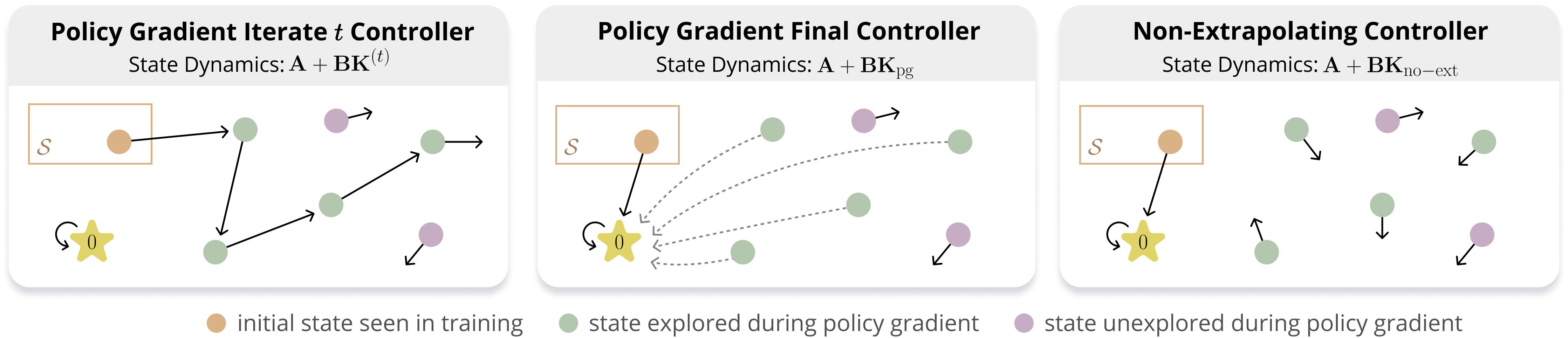
Figure 1: Intuition behind our theoretical analysis: in underdetermined LQR problems (Section 3.2), the extent to which a controller learned via policy gradient extrapolates to initial states unseen in training, depends on the degree of exploration induced by the system when commencing from initial states that were seen in training. Illustrated are the state dynamics induced by the $t$’th iterate of policy gradient ${\mathbf{K}}^{(t)}$ (left), by the final policy gradient controller ${\mathbf{K}}_{\mathrm{pg}}$ (middle), and by the non-extrapolating controller ${\mathbf{K}}_{\mathrm{no\text{-}ext}}$ defined in Section 3.3 (right). An arbitrary controller ${\mathbf{K}}$ extrapolates to initial states unseen in training if $\norm{({\mathbf{A}}+{\mathbf{B}}{\mathbf{K}}){\mathbf{x}}}^{2}$ is small for ${\mathbf{x}}\in{\mathcal{S}}^{\perp}$, i.e. if the dynamics induced by ${\mathbf{K}}$ send towards zero states that are orthogonal to the set ${\mathcal{S}}$ of initial states seen in training (see Section 3.3). Due to the structure of training cost gradients, the dynamics induced by the final policy gradient controller ${\mathbf{K}}_{\mathrm{pg}}$ send towards zero every state encountered in training. Accordingly, the extent to which ${\mathbf{K}}_{\mathrm{pg}}$ extrapolates depends on the degree of exploration — the overlap of states encountered in training with directions orthogonal to ${\mathcal{S}}$. On the other hand, the controller ${\mathbf{K}}_{\mathrm{no\text{-}ext}}$ ensures that states in ${\mathcal{S}}$ are sent to zero (thereby minimizing the training cost), but does not handle states in ${\mathcal{S}}^{\perp}$. It thus does not extrapolate.

4 Analysis of Implicit Bias

This section theoretically analyzes the extent to which policy gradient leads linear controllers in underdetermined LQR problems to extrapolate to initial states unseen in training.

4.1 Intuition: Extrapolation Depends on Exploration

Our analysis will reveal that the extent of extrapolation to initial states unseen in training depends on the degree of exploration induced by the system when commencing from initial states that were seen in training. Before going into the formal results, we provide intuition behind this dependence.

Per Equations 4 and 2, the training cost attained by a controller ${\mathbf{K}}$ can be written as follows:

$$J({\mathbf{K}};{\mathcal{S}})=c+\frac{1}{\abs{{\mathcal{S}}}}\sum\nolimits_{{\mathbf{x}}_{0}\in{\mathcal{S}}}\sum\nolimits_{h=1}^{H}\norm*{({\mathbf{A}}+{\mathbf{B}}{\mathbf{K}}){\mathbf{x}}_{h-1}}^{2}\text{\,,}$$

where $c>0$ does not depend on ${\mathbf{K}}$, and for each ${\mathbf{x}}_{0}\in{\mathcal{S}}$, the states ${\mathbf{x}}_{1},\ldots,{\mathbf{x}}_{H-1}$ are produced by the system when commencing from ${\mathbf{x}}_{0}$ and steered by ${\mathbf{K}}$.² Thus, minimizing the training cost amounts to finding a controller ${\mathbf{K}}$ such that $\norm{({\mathbf{A}}+{\mathbf{B}}{\mathbf{K}}){\mathbf{x}}}^{2}=0$ for every ${\mathbf{x}}$ belonging to a trajectory emanating from ${\mathcal{S}}$. Notice that it is possible to do so by simply ensuring that $\norm{({\mathbf{A}}+{\mathbf{B}}{\mathbf{K}}){\mathbf{x}}}^{2}=0$ for every ${\mathbf{x}}\in{\mathcal{S}}$. This is because, if $({\mathbf{A}}+{\mathbf{B}}{\mathbf{K}}){\mathbf{x}}={\mathbf{0}}$ for some ${\mathbf{x}}\in{\mathcal{S}}$, then all subsequent states in a trajectory emanating from ${\mathbf{x}}$ are zero.

As discussed in Section 3.3, for ${\mathbf{K}}$ to extrapolate to initial states unseen in training, we would like $\norm*{({\mathbf{A}}+{\mathbf{B}}{\mathbf{K}}){\mathbf{x}}}^{2}$ to be small for every ${\mathbf{x}}\in{\mathcal{U}}$, where ${\mathcal{U}}$ is an orthonormal basis for ${\mathcal{S}}^{\perp}$ (subspace orthogonal to the set ${\mathcal{S}}$ of initial states seen in training). We have seen in Section 3.3 that merely minimizing $\norm*{({\mathbf{A}}+{\mathbf{B}}{\mathbf{K}}){\mathbf{x}}}^{2}$ for every ${\mathbf{x}}\in{\mathcal{S}}$ implies nothing about the magnitude of this term for ${\mathbf{x}}\in{\mathcal{U}}$. In other words, it implies nothing about extrapolation.

Fortunately, it can be shown that the structure of $\nabla J(\cdot\,;{\mathcal{S}})$ is such that at every iteration $t\in{\mathbb{N}}$ of policy gradient (Equation 3), the iterates ${\mathbf{K}}^{(t)}$ and ${\mathbf{K}}^{(t+1)}$ tend to satisfy $\norm{({\mathbf{A}}+{\mathbf{B}}{\mathbf{K}}^{(t+1)}){\mathbf{x}}\big{\|}^{2}<\big{\|}({\mathbf{A}}+{\mathbf{B}}{\mathbf{K}}^{(t)}){\mathbf{x}}}^{2}$ for every state ${\mathbf{x}}$ along trajectories emanating from ${\mathcal{S}}$ that were encountered in the iteration, i.e. that have been steered by ${\mathbf{K}}^{(t)}$. Consequently, with ${\mathbf{K}}_{\mathrm{pg}}$ being a controller trained by policy gradient, $\norm*{({\mathbf{A}}+{\mathbf{B}}{\mathbf{K}}_{\mathrm{pg}}){\mathbf{x}}}^{2}$ is relatively small for every state ${\mathbf{x}}$ encountered in training (i.e. for every ${\mathbf{x}}$ belonging to a trajectory that was produced during training). The extent to which ${\mathbf{K}}_{\mathrm{pg}}$ extrapolates therefore depends on the degree of exploration — the overlap of states encountered in training with ${\mathcal{U}}$, i.e. with directions orthogonal to ${\mathcal{S}}$.

The above intuition is illustrated in Figure 1. The remainder of the section is devoted to its formalization.

4.2 Extrapolation Requires Exploration

The current subsection proves that in the absence of sufficient exploration, extrapolation to initial states unseen in training does not take place.

Recall from Section 3 that we consider a linear system defined by matrices ${\mathbf{A}}$ and ${\mathbf{B}}$, a set ${\mathcal{S}}$ of initial states seen in training, and a linear controller learned via policy gradient, whose iterates are denoted by ${\mathbf{K}}^{(t)}$ for $t\in{\mathbb{N}}$. Let ${\mathcal{X}}_{\mathrm{{pg}}}$ be the set of states encountered in training. More precisely, ${\mathcal{X}}_{\mathrm{{pg}}}$ is the union over ${\mathbf{x}}_{0}\in{\mathcal{S}}$ and $t\in{\mathbb{N}}$, of the states in the length $H$ trajectory emanating from ${\mathbf{x}}_{0}$ and steered by ${\mathbf{K}}^{(t)}$:

$${\mathcal{X}}_{\mathrm{{pg}}}:=$$ (10)

$$\brk[c]2{\!({\mathbf{A}}+{\mathbf{B}}{\mathbf{K}}^{(t)})^{h}{\mathbf{x}}_{0}:{\mathbf{x}}_{0}\in{\mathcal{S}},h\in\{0\}\cup[H-1],t\in{\mathbb{N}}}\text{.}$$

Proposition 1 below establishes that the learned controller can only extrapolate to initial states spanned by ${\mathcal{X}}_{\mathrm{{pg}}}$. More precisely, for any $t\in{\mathbb{N}}$ and ${\mathbf{x}}\in{\mathcal{X}}_{\mathrm{{pg}}}^{\perp}$, the controller ${\mathbf{K}}^{(t)}$ assigns to ${\mathbf{x}}$ a trivial control of zero. This implies that if ${\mathcal{X}}_{\mathrm{{pg}}}\subseteq\mathrm{span}({\mathcal{S}})$, meaning no state outside $\mathrm{span}({\mathcal{S}})$ is encountered in training, then the optimality extrapolation measure of ${\mathbf{K}}^{(t)}$ is trivial, i.e. equal to that of ${\mathbf{K}}_{\mathrm{no\text{-}ext}}$ (see Section 3.3). Proposition 1 further shows that such non-exploratory settings exist — there exist systems (matrices ${\mathbf{A}}$ and ${\mathbf{B}}$) with which, for any choice of ${\mathcal{S}}$, it holds that ${\mathcal{X}}_{\mathrm{{pg}}}\subseteq\mathrm{span}({\mathcal{S}})$. In the exemplified settings, similarly to the optimality extrapolation measure, the cost extrapolation measure of ${\mathbf{K}}^{(t)}$ is trivial (and greater than zero).

Proposition 1.

For any iteration $t\in{\mathbb{N}}$ of policy gradient, the following hold.

• (Exploration is necessary for extrapolation) For any ${\mathbf{x}}\in{\mathcal{X}}_{\mathrm{{pg}}}^{\perp}$ it holds that ${\mathbf{K}}^{(t)}{\mathbf{x}}={\mathbf{0}}$. Consequently, if ${\mathcal{X}}_{\mathrm{{pg}}}\subseteq\mathrm{span}({\mathcal{S}})$ then ${\mathcal{E}}_{\mathrm{opt}}({\mathbf{K}}^{(t)})={\mathcal{E}}_{\mathrm{opt}}({\mathbf{K}}_{\mathrm{no\text{-}ext}})$.

• (Existence of non-exploratory settings) There exist system matrices ${\mathbf{A}}$ and ${\mathbf{B}}$ such that, for any set ${\mathcal{S}}$ of initial states seen in training: ${\mathcal{X}}_{\mathrm{{pg}}}\subseteq\mathrm{span}({\mathcal{S}})$; and:

  $$\begin{split}{\mathcal{E}}_{\mathrm{opt}}({\mathbf{K}}^{(t)})&={\mathcal{E}}_{\mathrm{opt}}({\mathbf{K}}_{\mathrm{no\text{-}ext}})=1\text{\,,}\\[3.00003pt] {\mathcal{E}}_{\mathrm{cost}}({\mathbf{K}}^{(t)})&={\mathcal{E}}_{\mathrm{cost}}({\mathbf{K}}_{\mathrm{no\text{-}ext}})=H\text{\,,}\end{split}$$

  where recall $H$ is the horizon.

Proof sketch (proof in Section D.2).

We establish that for any ${\mathbf{K}}\in{\mathbb{R}}^{D\times D}$, the rows of $\nabla J({\mathbf{K}};{\mathcal{S}})$ are spanned by states in the trajectories that emanate from ${\mathcal{S}}$ and are steered by ${\mathbf{K}}$. Since ${\mathbf{K}}^{(1)}={\mathbf{0}}$, it follows that for any $t\in{\mathbb{N}}$, the rows of ${\mathbf{K}}^{(t)}$ are spanned by ${\mathcal{X}}_{\mathrm{{pg}}}$, and so ${\mathbf{K}}^{(t)}{\mathbf{x}}={\mathbf{0}}$ for any ${\mathbf{x}}\in{\mathcal{X}}_{\mathrm{{pg}}}^{\perp}$. If ${\mathcal{X}}_{\mathrm{{pg}}}\subseteq\mathrm{span}({\mathcal{S}})$ then this immediately implies that the optimality measure attained by ${\mathbf{K}}^{(t)}$ is equal to that of ${\mathbf{K}}_{\mathrm{no\text{-}ext}}$.

As for existence of non-exploratory settings, suppose that ${\mathbf{A}}={\mathbf{B}}={\mathbf{I}}$, where ${\mathbf{I}}$ is the identity matrix. With arbitrary ${\mathcal{S}}$, we prove that ${\mathcal{X}}_{\mathrm{{pg}}}\subseteq\mathrm{span}({\mathcal{S}})$ by showing that the state dynamics induced by ${\mathbf{A}},{\mathbf{B}},$ and ${\mathbf{K}}^{(t)}$ are invariant to $\mathrm{span}({\mathcal{S}})$, i.e. $({\mathbf{A}}+{\mathbf{B}}{\mathbf{K}}^{(t)}){\mathbf{x}}\in\mathrm{span}({\mathcal{S}})$ if ${\mathbf{x}}\in\mathrm{span}({\mathcal{S}})$. Then, by the first part of the proposition, ${\mathcal{X}}_{\mathrm{{pg}}}\subseteq\mathrm{span}({\mathcal{S}})$ implies that ${\mathbf{K}}^{(t)}{\mathbf{x}}={\mathbf{0}}$ for any ${\mathbf{x}}\in{\mathcal{U}}$. The same is true for ${\mathbf{K}}_{\mathrm{no\text{-}ext}}$. Hence, ${\mathbf{A}}+{\mathbf{B}}{\mathbf{K}}^{(t)}$ and ${\mathbf{A}}+{\mathbf{B}}{\mathbf{K}}_{\mathrm{no\text{-}ext}}$ both map any ${\mathbf{x}}\in{\mathcal{U}}$ back to itself. Using this observation, the optimality and cost measures of extrapolation attained by ${\mathbf{K}}^{(t)}$ and ${\mathbf{K}}_{\mathrm{no\text{-}ext}}$ are readily computed. ∎

Remark 1.

The first part of Proposition 1 (exploration is necessary for extrapolation) extends to the setting where ${\mathbf{B}}\in{\mathbb{R}}^{D\times D}$ is arbitrary and ${\mathbf{Q}}\in{\mathbb{R}}^{D\times D}$ is any positive semidefinite matrix. The proof in Section D.2 accounts for this more general setting.

4.3 Extrapolation in Exploration-Inducing Setting

Section 4.2 proved that, in the absence of sufficient exploration, extrapolation to initial states unseen in training does not take place. We now show that with sufficient exploration, extrapolation can take place. Namely, we construct a system that encourages exploration when commencing from a given initial state, and show that with this system and initial state, training via policy gradient leads to extrapolation, which — depending on characteristics of the cost — varies between partial and perfect.

Suppose that we are given an initial state seen in training, which, without loss of generality, is the standard basis vector ${\mathbf{e}}_{1}\in{\mathbb{R}}^{D}$. Assume for simplicity that the horizon $H$ is divisible by the state space dimension $D$. When commencing from ${\mathbf{e}}_{1}$ and steered by the first iterate of policy gradient, i.e. by ${\mathbf{K}}^{(1)}={\mathbf{0}}$, the system produces the length $H$ trajectory $\mathcal{T}:=({\mathbf{e}}_{1},{\mathbf{A}}{\mathbf{e}}_{1},\ldots,{\mathbf{A}}^{H-1}{\mathbf{e}}_{1})$. In light of Section 4.2, for encouraging exploration we would like the states in $\mathcal{T}$ to span the entire state space. A simple choice that ensures this is ${\mathbf{A}}={\mathbf{A}}_{\mathrm{shift}}:=\sum\nolimits_{d=1}^{D}{\mathbf{e}}_{d\%D+1}{\mathbf{e}}_{d}^{\top}$. Under this choice, $\mathcal{T}$ cyclically traverses through the standard basis vectors ${\mathbf{e}}_{1},\ldots,{\mathbf{e}}_{D}$.

Proposition 2 below establishes that, in the setting under consideration, the implicit bias of policy gradient leads to extrapolation. Specifically, the learned controller attains optimality and cost measures of extrapolation that are substantially less than those of ${\mathbf{K}}_{\mathrm{no\text{-}ext}}$ (see Section 3.3). This phenomenon is more potent the longer the horizon $H$ is, with perfect extrapolation attained in the limit $H\to\infty$.

Proposition 2.

Assume that ${\mathcal{S}}=\brk[c]{{\mathbf{e}}_{1}}$, ${\mathbf{A}}={\mathbf{A}}_{\mathrm{shift}}$, and $H$ is divisible by $D$. Then, policy gradient with learning rate $\eta=\brk 1{H^{2}/D+H}^{-1}$ converges to a controller ${\mathbf{K}}_{\mathrm{pg}}$ that: (i) minimizes the training cost, i.e. $J({\mathbf{K}}_{\mathrm{pg}};{\mathcal{S}})=J^{*}({\mathcal{S}})$; and (ii) satisfies:

$$\begin{split}\frac{{\mathcal{E}}_{\mathrm{opt}}\brk 1{{\mathbf{K}}_{\mathrm{pg}}}}{{\mathcal{E}}_{\mathrm{opt}}\brk*{{\mathbf{K}}_{\mathrm{no\text{-}ext}}}}&\leq\frac{4(D-1)^{2}}{(H+D)^{2}}\text{\,,}\\[5.0pt] \frac{{\mathcal{E}}_{\mathrm{cost}}({\mathbf{K}}_{\mathrm{pg}})}{{\mathcal{E}}_{\mathrm{cost}}({\mathbf{K}}_{\mathrm{no\text{-}ext}})}&\leq\frac{4(D-1)^{2}}{(H+D)^{2}}\text{\,.}\end{split}$$

Proof sketch (proof in Section D.3).

The analysis follows from first principles, building on a particularly lucid form that $\nabla J({\mathbf{K}}^{(1)};{\mathcal{S}})$ takes. Specifically, we derive an explicit expression for ${\mathbf{K}}^{(2)}$, and show that it minimizes the training cost via the optimality condition of Equation 5. This implies that policy gradient converges to ${\mathbf{K}}_{\mathrm{pg}}={\mathbf{K}}^{(2)}$. Extrapolation in terms of the optimality and cost measures then follows from the derived expression for ${\mathbf{K}}^{(2)}$. ∎

Remark 2.

Appendix B generalizes Proposition 2 to the setting where ${\mathbf{Q}}$ is any diagonal positive semidefinite matrix. The generalized analysis sheds light on how ${\mathbf{Q}}$ impacts extrapolation. In particular, it shows that for certain values of ${\mathbf{Q}}$, extrapolation can be perfect even with a finite horizon $H$.

4.3.1 Implicit Bias in Optimal Control $\neq$ Euclidean Norm Minimization

A widely known fact is that in supervised learning, when labels are continuous (regression) and the training objective is underdetermined, gradient descent over linear predictors implicitly minimizes the Euclidean norm. That is, among all predictors minimizing the training objective, gradient descent converges to the one whose Euclidean norm is minimal (cf. Zhang et al. (2017)). A perhaps surprising implication of Proposition 2, formalized by Lemmas 1 and 1 below, is that an analogous phenomenon does not take place in optimal control. In fact, the (unique) minimal Euclidean norm controller, among those minimizing the training cost, is the non-extrapolating ${\mathbf{K}}_{\mathrm{no\text{-}ext}}$. Thus, the extrapolation guarantee of Proposition 2 implies that policy gradient over a linear controller does not implicitly minimize the Euclidean norm. This finding highlights that conventional wisdom regarding implicit bias in supervised learning cannot be blindly applied to optimal control. We hope it will encourage further research dedicated to implicit bias in optimal control.

Lemma 1.

Of all controllers minimizing the training cost, i.e. all ${\mathbf{K}}\in{\mathcal{K}}_{\mathcal{S}}$ (Equation 7), the non-extrapolating ${\mathbf{K}}_{\mathrm{no\text{-}ext}}$ is the unique one with minimal Euclidean norm.

Proof sketch (proof in Section D.4).

Through the method of Lagrange multipliers, we show that if the rows of some ${\mathbf{K}}\in{\mathcal{K}}_{\mathcal{S}}$ are in $\mathrm{span}({\mathcal{S}})$, then ${\mathbf{K}}$ is the unique member of ${\mathcal{K}}_{\mathcal{S}}$ whose Euclidean norm is minimal. We then show that the rows of ${\mathbf{K}}_{\mathrm{no\text{-}ext}}$ necessarily reside in $\mathrm{span}({\mathcal{S}})$. ∎

Corollary 1.

In the setting of Proposition 2, ${\mathbf{K}}_{\mathrm{pg}}$ — the controller to which policy gradient converges, and which minimizes the training cost — satisfies:

$$\norm*{{\mathbf{K}}_{\mathrm{pg}}}^{2}-\min\nolimits_{{\mathbf{K}}\in{\mathcal{K}}_{\mathcal{S}}}\norm{{\mathbf{K}}}^{2}=\sum\nolimits_{d=2}^{D}\brk*{1-\frac{2(d-1)}{H+D}}^{2}\text{,}$$

where note that the right hand side is $\Omega(D)$.

Proof sketch (proof in Section D.5).

We derive an expression for ${\mathbf{K}}_{\mathrm{no\text{-}ext}}$ to compute its squared Euclidean norm, which by Lemma 1 is equal to $\min\nolimits_{{\mathbf{K}}\in{\mathcal{K}}_{\mathcal{S}}}\norm{{\mathbf{K}}}^{2}$. Then, an expression for ${\mathbf{K}}_{\mathrm{pg}}$, established as a lemma in the proof of Proposition 2, yields the desired result. ∎

4.4 Extrapolation in Typical Setting

Sections 4.2 and 4.3 presented two ends of a spectrum. On one end, Section 4.2 proved that, in the absence of sufficient exploration, extrapolation to initial states unseen in training does not take place. On the other end, Section 4.3 constructed an exploration-inducing setting (namely, a system for a given initial state seen in training), and showed that it leads to extrapolation, which — depending on characteristics of the cost — varies between partial and perfect. A natural question is what extrapolation may be expected in a typical setting.

We address the foregoing question by considering an arbitrary (non-zero) initial state seen in training ${\mathbf{x}}_{0}\in{\mathbb{R}}^{D}$ — which without loss of generality is assumed to have unit norm  — and a randomly generated system matrix ${\mathbf{A}}$. For the randomness of ${\mathbf{A}}$, we draw entries independently from a Gaussian distribution with mean zero and standard deviation $1/\sqrt{D}$. This choice of standard deviation is common in the literature on random matrix theory (Anderson et al., 2010), and ensures that with high probability, the spectral norm of ${\mathbf{A}}$ is roughly constant, i.e. independent of the state space dimension $D$ (cf. Theorem 4.4.5 in Vershynin (2020)). When commencing from ${\mathbf{x}}_{0}$ and steered by the first iterate of policy gradient, i.e. by ${\mathbf{K}}^{(1)}={\mathbf{0}}$, the system produces the length $D$ trajectory $({\mathbf{x}}_{0},{\mathbf{A}}{\mathbf{x}}_{0},\ldots,{\mathbf{A}}^{D-1}{\mathbf{x}}_{0})$. Since ${\mathbf{x}}_{0}$ is a cyclic vector of ${\mathbf{A}}$ almost surely (see Appendix C for a proof of this fact), the latter trajectory spans the entire state space almost surely. The necessary condition for extrapolation put forth in Section 4.2 is thus supported, implying that extrapolation could take place.

Theorem 1 below establishes that a single iteration of policy gradient already leads — in expectation, and with high probability if the state space dimension is large — to non-trivial extrapolation, as quantified by the optimality measure. The theorem overcomes considerable technical challenges (arising from the complexity of random systems) via advanced tools from the intersection of random matrix theory and topology. These tools may be of independent interest.

Theorem 1.

Let ${\mathbf{x}}_{0}\in{\mathbb{R}}^{D}$ be an arbitrary unit vector. Assume that the set ${\mathcal{S}}$ of initial states seen in training consists of ${\mathbf{x}}_{0}$ (i.e. ${\mathcal{S}}=\brk[c]{{\mathbf{x}}_{0}}$), that the entries of ${\mathbf{A}}$ are drawn independently from a Gaussian distribution with mean zero and standard deviation $1/\sqrt{D}$, and that the horizon $H$ is greater than one. Then, with learning rate $\eta\leq\frac{1}{4DH(H-1)(4H-1)!!}$, where $N!!:=N(N-2)(N-4)\cdots 3$ is the double factorial of an odd $N\in{\mathbb{N}}$, the second iterate of policy gradient, i.e. ${\mathbf{K}}^{(2)}$, satisfies:

$$\frac{\mathop{\mathbb{E}}_{{\mathbf{A}}}\brk[s]*{{\mathcal{E}}_{\mathrm{opt}}\brk*{{\mathbf{K}}^{(2)}}}}{\mathop{\mathbb{E}}_{{\mathbf{A}}}\brk[s]*{{\mathcal{E}}_{\mathrm{opt}}\brk*{{\mathbf{K}}_{\mathrm{no\text{-}ext}}}}}\leq 1-\eta\cdot\frac{H(H-1)}{D}\text{\,,}$$

where ${\mathbf{K}}_{\mathrm{no\text{-}ext}}$ is the non-extrapolating controller defined in Section 3.3. Moreover, for any $\delta\in(0,1)$, if $D\geq\abs{{\mathcal{S}}}+\frac{6\abs{{\mathcal{S}}}H(H-1)(4H-1)!!}{\delta}$ and $\eta\leq\frac{1}{8D^{2}H(H-1)(4H-1)!!}$, then with probability at least $1-\delta$ over the choice of ${\mathbf{A}}$:

$$\frac{{\mathcal{E}}_{\mathrm{opt}}\brk*{{\mathbf{K}}^{(2)}}}{{\mathcal{E}}_{\mathrm{opt}}\brk*{{\mathbf{K}}_{\mathrm{no\text{-}ext}}}}\leq 1-\eta\cdot\frac{H(H-1)}{4D}\text{\,.}$$

Lastly, the above results hold even if we replace ${\mathcal{S}}$ by an arbitrary set of orthonormal vectors.

Proof sketch (proof in Section D.8).

The intuition behind the proof (valid for $H\geq D$) is as follows. As stated in the discussion regarding exploration at the opening of this subsection, almost surely, the length $D$ trajectory steered by the first iterate of policy gradient, i.e. by ${\mathbf{K}}^{(1)}$, spans the entire state space. Therefore, almost surely, states encountered in training overlap with ${\mathcal{U}}$, i.e. with directions orthogonal to ${\mathcal{S}}$ (see Section 3.3). The intuitive arguments in Section 4.1 thus suggest that extrapolation will take place.

Converting the above intuition into a formal proof entails considerable technical challenges. We address these challenges by employing advanced tools from the intersection of random matrix theory and topology. Specifically, we employ a method from Redelmeier (2014) for computing expectations of traces of random matrix products, through the topological concept of genus expansion. For the convenience of the reader, a detailed outline of the proof is provided in Section D.8. ∎

Limitations. Despite overcoming considerable technical challenges, Theorem 1 remains limited in three ways: (i) the requirement from the learning rate $\eta$, and the requirement from the state space dimension $D$ in the second (high probability) result, depend on $(4H-1)!!$, which grows super exponentially with the horizon $H$; (ii) extrapolation guarantees are provided only for the first iteration of policy gradient; and (iii) in contrast to the analyses of Sections 4.2 and 4.3, extrapolation results apply only to the optimality measure, not to the cost measure. Experiments reported in Section 5.1 suggest that all three limitations above may be alleviated. Doing so is regarded as a valuable direction for future work.

5 Experiments

In this section, we corroborate our theory (Section 4) via experiments, demonstrating how the interplay between a system and initial states seen in training affects the extent to which a controller learned via policy gradient extrapolates to initial states unseen in training. Section 5.1 presents experiments with the analyzed underdetermined LQR problems, after which Section 5.2 considers non-linear systems and (non-linear) neural network controllers. For conciseness, we defer some experiments and implementation details to Appendix E. Code for reproducing our experiments is available at https://github.com/noamrazin/imp_bias_control.

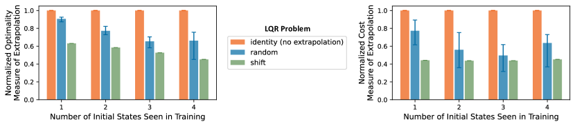
Figure 2: In underdetermined LQR problems (Section 3.2), the extent to which linear controllers learned via policy gradient extrapolate to initial states unseen in training, depends on the degree of exploration that the system induces from initial states that were seen in training. We evaluated LQR problems with state space dimension $D=5$, horizon $H=5$, and three different linear systems: (i) an “identity” system with ${\mathbf{A}}={\mathbf{I}}\in{\mathbb{R}}^{D\times D}$ (analyzed in Section 4.2); (ii) a “shift” system with ${\mathbf{A}}=\sum\nolimits_{d=1}^{D}{\mathbf{e}}_{d\%D+1}{\mathbf{e}}_{d}^{\top}$ (analyzed in Section 4.3); and (iii) a random system, where the entries of ${\mathbf{A}}$ are sampled independently from a zero-mean Gaussian with standard deviation $1/\sqrt{D}$ (analyzed in Section 4.4). Reported are the optimality (Definition 1) and cost (Definition 2) measures of extrapolation, normalized by the respective quantities attained by the non-extrapolating controller ${\mathbf{K}}_{\mathrm{no\text{-}ext}}$ (see Section 3.3). A value of one corresponds to trivial (no) extrapolation and a value of zero corresponds to perfect extrapolation. Bar heights stand for median values over $20$ runs differing in random seed, and error bars span the interquartile range ($25$’th to $75$’th percentiles). Results: In agreement with our theory (Sections 4.2, 4.3, and 4.4), no extrapolation takes place under the “identity” system, since it does not induce exploration from initial states seen in training. On the other hand, substantial, yet far from perfect extrapolation is achieved under the “shift” and random systems, which induce exploration. Note that this accords with the results of Section 4.3, as they indicate that extrapolation is usually not perfect.

5.1 Linear Quadratic Control

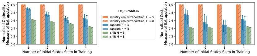
Figure 4: In underdetermined LQR problems (Section 3.2), the extent to which linear controllers learned via policy gradient extrapolate to initial states unseen in training, depends on the degree of exploration that the system induces from initial states that were seen in training. This figure supplements Figure 2 by including results for analogous experiments over systems with a longer time horizon $H=8$ (instead of $H=5$). Results: The increase in time horizon improved extrapolation to unseen initial states, in accordance with the analysis of Section 4.3. A drawback of increasing the time horizon, however, is that it can lead to instabilities during training (cf. Metz et al. (2021)). Indeed, we were unable to consistently train controllers when the time horizon was substantially longer than $H=8$. Thus, techniques enabling stable training with long time horizons may be a promising tool for improving extrapolation.

Our theoretical analysis considered underdetermined LQR problems in three settings, respectively comprising: (i) systems that do not induce exploration from any initial states (Section 4.2); (ii) systems with a “shift” transition matrix ${\mathbf{A}}$, which induce exploration from certain initial states (Section 4.3); and (iii) systems with a randomly generated ${\mathbf{A}}$, which induce exploration from any initial states (Section 4.4). According to our analysis, with systems that do not induce exploration from initial states seen in training, controllers trained via policy gradient do not extrapolate. On the other hand, non-trivial extrapolation occurs under “shift” and random systems. Figure 2 demonstrates these findings empirically, showcasing the relation between the system and extrapolation to initial states unseen in training. Figures 4 and 5 in Section E.1 provide additional experiments in settings with, respectively: (i) a longer time horizon; and (ii) random ${\mathbf{B}}$ and ${\mathbf{Q}}$ matrices.

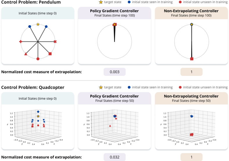
Figure 3: In the pendulum and quadcopter control problems (see Section 5.2), a (non-linear) neural network controller trained via policy gradient often extrapolates to initial states unseen in training, despite the existence of non-extrapolating controllers. Left: Initial states seen in training (blue) and initial states unseen in training that are used for evaluating extrapolation (red). Middle: States at the final time step when controlling the system using a (state-feedback) controller learned via policy gradient. The controller is parameterized as a fully-connected neural network with ReLU activation. We carried out five training runs with different random seeds, and chose to display the controller that attained the median cost measure of extrapolation. Right: States at the final time step when controlling the system using a non-extrapolating controller, i.e. a controller that minimizes the cost for initial states seen in training while performing poorly on initial states unseen in training. We obtained such a controller by employing a modified training objective that encourages steering unseen initial states to a state different than the target state. Results: Since an uncontrolled pendulum or quadcopter falls downwards from a given initial state, the systems qualitatively induce exploration of states with lower height. Complying with our theory for LQR problems (Section 4), policy gradient yields near-perfect extrapolation to unseen initial states lower that those used for training. In particular, the cost measure of extrapolation, normalized by that attained by the non-extrapolating controller, is near the minimal value of zero (a value of one stands for no extrapolation). Further details in Appendix E: Tables 1 and 2 fully specify the initial and final states depicted above, and Figures 6 and 7 present the evolution of states through time under the policy gradient and non-extrapolating controllers.

5.2 Non-Linear Systems and Neural Network Controllers

The LQR problem is of central theoretical and practical importance in optimal control (Anderson & Moore, 2007). For example, it supports controlling non-linear systems via iterative linearizations (Li & Todorov, 2004). An alternative approach to controlling non-linear systems is to train (non-linear) neural network controllers via policy gradient. This approach is largely motivated by the success of neural networks in supervised learning, and has gained significant interest in recent years (see, e.g., Hu et al. (2019); Qiao et al. (2020); Clavera et al. (2020); Mora et al. (2021); Gillen & Byl (2022); Howell et al. (2022); Xu et al. (2022); Wiedemann et al. (2023)).

Our analysis of underdetermined LQR problems (Section 4) implies that, when a linear system induces exploration from initial states seen in training, a linear controller trained via policy gradient typically extrapolates to initial states unseen in training. The current subsection empirically demonstrates that this phenomenon extends to non-linear systems and neural network controllers. Experiments include two non-linear control problems, in which the goal is to steer either a pendulum or quadcopter towards a target state.

The pendulum control problem. A classic non-linear control problem is that of stabilizing a (simulated) pendulum at an upright position (cf. Hazan & Singh (2022)). At time step $h$, the two-dimensional state of the system is described by the vertical angle of the pendulum $\theta_{h}\in{\mathbb{R}}$ and its angular velocity $\dot{\theta}_{h}\in{\mathbb{R}}$. The controller applies a torque $u_{h}\in{\mathbb{R}}$, with the goal of making the pendulum reach and stay at the target state $(\pi,0)$. Accordingly, the cost at each time step is the squared Euclidean distance between the current and target states. See Section E.3.2 for explicit equations defining the state dynamics and cost.

The quadcopter control problem. Another common non-linear control problem is that of controlling a (simulated) quadcopter (cf. Panerati et al. (2021)). At time step $h$, the state of the system ${\mathbf{x}}_{h}\in{\mathbb{R}}^{12}$ comprises the quadcopter’s position $(x_{h},y_{h},z_{h})\in{\mathbb{R}}^{3}$, tilt angles $(\phi_{h},\theta_{h},\psi_{h})\in{\mathbb{R}}^{3}$ (i.e. roll, pitch, and yaw), and their respective velocities. The controller determines the revolutions per minute (RPM) for each of the four motors by choosing ${\mathbf{u}}_{h}\in[0,\text{MAX\_RPM}]^{4}$, where MAX_RPM stands for the maximal supported RPM. We consider the goal of making the quadcopter reach and stay at the target state ${\mathbf{x}}^{*}=(0,0,1,0,\ldots,0)$. This is expressed by taking the cost at each time step to be a weighted squared Euclidean distance between the current and target states. See Section E.3.3 for explicit equations defining the state dynamics and cost.

Results. For both the pendulum and quadcopter control problems, we train via policy gradient a (state-feedback) controller, parameterized as a fully-connected neural network with ReLU activation. The controls produced by a randomly initialized neural network are usually near zero. Hence, during the first iterations of policy gradient, both the pendulum and quadcopter fall downwards from their respective initial states, qualitatively leading to exploration. Figure 3 shows that, in accordance with our theory for LQR problems, in both the pendulum and quadcopter problems, when training with initial states of some height, the controller can extrapolate near-perfectly to unseen initial states of lower height. The extrapolation is observed qualitatively, in terms of the final states in a trajectory being near the target state, and quantitatively, as evaluated by the cost measure compared to a non-extrapolating controller. Moreover, for the quadcopter control problem, Figures 8 and 10 in Section E.2 demonstrate that, respectively: (i) the extent of extrapolation varies depending on the distance from initial states seen in training; and (ii) extrapolation also applies to unseen initial states with horizontal distance from the initial states seen in training.

6 Conclusion

The implicit bias of gradient descent is a cornerstone of modern machine learning. While extensively studied in supervised learning, it is far less understood in optimal control (reinforcement learning). There, learning a controller applied to a system via gradient descent is known as policy gradient, and a question of prime importance (particularly for safety-critical applications, e.g. robotics, industrial manufacturing, or autonomous driving) is the extent to which a learned controller extrapolates to initial states unseen in training. In this paper we theoretically studied the implicit bias of policy gradient in terms of extrapolation to initial states unseen in training. Focusing on the fundamental LQR problem, we established that the extent of extrapolation depends on the degree of exploration induced by the system when commencing from initial states included in training. Experiments corroborated our theory, and demonstrated its conclusions on problems beyond LQR, where systems are non-linear and controllers are neural networks.

Future work includes extending our theory in three ways. First, is to alleviate the technical limitations specified in Section 4.4. Second, is to account for non-linear systems and neural network controllers such as those evaluated in our experiments. Third, is to address settings where systems are unknown or non-differentiable, and gradients with respect to controller parameters are estimated via sampling.

An additional direction for future research, which we hope our work will inspire, is the development of practical methods for selecting initial states whose inclusion in training enhances extrapolation to initial states unseen in training. In real-world optimal control (and reinforcement learning), with contemporary learning algorithms, extrapolation to initial states unseen in training is often poor (Rajeswaran et al., 2017; Zhang et al., 2018, 2019; Fujimoto et al., 2019; Witty et al., 2021). We believe methods as described bear potential to greatly improve it.

References

Appendix A Extrapolation Measures Are Invariant to the Choice of Orthonormal Basis

This appendix establishes that the optimality and cost measures of extrapolation (Definitions 1 and 2 in Section 3.3, respectively) are invariant to the choice of orthonormal basis ${\mathcal{U}}$ for ${\mathcal{S}}^{\perp}$, where ${\mathcal{S}}^{\perp}$ is the subspace orthogonal to the set ${\mathcal{S}}$ of initial states seen in training. That is, for any two such orthonormal bases ${\mathcal{U}}$ and ${\mathcal{U}}^{\prime}$, the respective values of the optimality and cost measures are the same.

Lemma 2.

For any controller ${\mathbf{K}}\in{\mathbb{R}}^{D\times D}$, the optimality and cost measures of extrapolation are invariant to the choice of orthonormal basis ${\mathcal{U}}$ for ${\mathcal{S}}^{\perp}$.

Proof.

Let ${\mathcal{U}}$ be an orthonormal basis of ${\mathcal{S}}^{\perp}$, and denote by ${\mathbf{V}}\in{\mathbb{R}}^{D\times\abs{{\mathcal{U}}}}$ the matrix whose columns are the initial states in ${\mathcal{U}}$. Furthermore, let ${\mathbf{Z}}\in{\mathbb{R}}^{D\times\dim(\mathrm{span}({\mathcal{S}}))}$ be a matrix whose columns form an orthonormal basis for $\mathrm{span}({\mathcal{S}})$. Notice that the concatenated matrix $[{\mathbf{V}},{\mathbf{Z}}]\in{\mathbb{R}}^{D\times D}$ is an orthogonal matrix.

Now, for ${\mathbf{K}}\in{\mathbb{R}}^{D\times D}$, the optimality measure of extrapolation can be written in a matricized form as follows:

$${\mathcal{E}}_{\mathrm{opt}}({\mathbf{K}})=\frac{1}{\abs{{\mathcal{U}}}}\norm*{({\mathbf{A}}+{\mathbf{B}}{\mathbf{K}}){\mathbf{V}}}^{2}=\frac{1}{\abs{{\mathcal{U}}}}\brk*{\norm*{({\mathbf{A}}+{\mathbf{B}}{\mathbf{K}})[{\mathbf{V}},{\mathbf{Z}}]}^{2}-\norm*{({\mathbf{A}}+{\mathbf{B}}{\mathbf{K}}){\mathbf{Z}}}^{2}}\text{\,.}$$

Since the Euclidean norm is orthogonally invariant, we get that:

$${\mathcal{E}}_{\mathrm{opt}}({\mathbf{K}})=\frac{1}{\abs{{\mathcal{U}}}}\brk*{\norm*{{\mathbf{A}}+{\mathbf{B}}{\mathbf{K}}}^{2}-\norm*{({\mathbf{A}}+{\mathbf{B}}{\mathbf{K}}){\mathbf{Z}}}^{2}}\text{\,.}$$

As can be seen in the expression above, the optimality measure of extrapolation does not depend on the choice of ${\mathcal{U}}$.

Similarly, for ${\mathbf{K}}\in{\mathbb{R}}^{D\times D}$, the cost measure of extrapolation can be written in a matricized form as follows:

$$\begin{split}{\mathcal{E}}_{\mathrm{cost}}({\mathbf{K}})&=J({\mathbf{K}};{\mathcal{U}})-J^{*}({\mathcal{U}})\\ &=\frac{1}{\abs{{\mathcal{U}}}}\sum\nolimits_{h=0}^{H}\norm*{({\mathbf{A}}+{\mathbf{B}}{\mathbf{K}})^{h}{\mathbf{V}}}^{2}-1\\ &=\frac{1}{\abs{{\mathcal{U}}}}\sum\nolimits_{h=1}^{H}\norm*{({\mathbf{A}}+{\mathbf{B}}{\mathbf{K}})^{h}{\mathbf{V}}}^{2}\\ &=\frac{1}{\abs{{\mathcal{U}}}}\sum\nolimits_{h=1}^{H}\brk*{\norm*{({\mathbf{A}}+{\mathbf{B}}{\mathbf{K}})^{h}[{\mathbf{V}},{\mathbf{Z}}]}^{2}-\norm*{({\mathbf{A}}+{\mathbf{B}}{\mathbf{K}})^{h}{\mathbf{Z}}}^{2}}\text{\,,}\end{split}$$

where we used the fact that $J^{*}({\mathcal{X}})=1$ for any finite set of unit norm initial states ${\mathcal{X}}\subset{\mathbb{R}}^{D}$. Again, since the Euclidean norm is orthogonally invariant, we get an expression for ${\mathcal{E}}_{\mathrm{cost}}({\mathbf{K}})$ that does not depend on the choice of ${\mathcal{U}}$:

$${\mathcal{E}}_{\mathrm{cost}}({\mathbf{K}})=\frac{1}{\abs{{\mathcal{U}}}}\sum\nolimits_{h=1}^{H}\brk*{\norm*{({\mathbf{A}}+{\mathbf{B}}{\mathbf{K}})^{h}}^{2}-\norm*{({\mathbf{A}}+{\mathbf{B}}{\mathbf{K}})^{h}{\mathbf{Z}}}^{2}}\text{\,.}$$

∎

Appendix B Extension of Analysis for Exploration-Inducing Setting to Diagonal ${\mathbf{Q}}$

In this appendix, we generalize the analysis of the exploration-inducing setting from Section 4.3 to the case where ${\mathbf{Q}}$ is a general diagonal positive semidefinite matrix (not necessarily the identity matrix ${\mathbf{I}}$). The generalized analysis sheds light on how ${\mathbf{Q}}$ impacts extrapolation. In particular, it shows that for certain values of ${\mathbf{Q}}$ extrapolation can be perfect even for a finite horizon $H$ (recall that, as shown in Section 4.3, when ${\mathbf{Q}}={\mathbf{I}}$ perfect extrapolation in the setting considered therein is attained only when $H\to\infty$).

Let ${\mathbf{Q}}\in{\mathbb{R}}^{D\times D}$ be a diagonal positive semidefinite matrix with diagonal entries $q_{1},\ldots,q_{D}\geq 0$, and assume that $q_{j}>0$ for at least some $j\in[D]$ (otherwise, the problem is trivial — the cost for any controller and initial state is zero). For such ${\mathbf{Q}}$, the cost in an underdetermined LQR problem (Equation 4), attained by a controller ${\mathbf{K}}\in{\mathbb{R}}^{D\times D}$ over a finite set ${\mathcal{X}}\subset{\mathbb{R}}^{D}$ of initial states, can be written as:

$$J({\mathbf{K}};{\mathcal{X}})=\frac{1}{\abs{{\mathcal{X}}}}\sum\nolimits_{{\mathbf{x}}_{0}{\mathcal{X}}}\sum\nolimits_{h=0}^{H}\norm*{({\mathbf{A}}+{\mathbf{B}}{\mathbf{K}})^{h}{\mathbf{x}}_{0}}_{\mathbf{Q}}^{2}\text{\,,}$$ (11)

where $\norm{{\mathbf{v}}}_{{\mathbf{Q}}}:=\sqrt{{\mathbf{v}}^{\top}{\mathbf{Q}}{\mathbf{v}}}$ for ${\mathbf{v}}\in{\mathbb{R}}^{D}$. The global minimum of this cost is:

$$J^{*}({\mathcal{X}}):=\min\nolimits_{{\mathbf{K}}\in{\mathbb{R}}^{D\times D}}J({\mathbf{K}};{\mathcal{X}})=\frac{1}{\abs{{\mathcal{X}}}}\sum\nolimits_{{\mathbf{x}}_{0}\in{\mathcal{X}}}\norm{{\mathbf{x}}_{0}}_{\mathbf{Q}}^{2}\text{\,,}$$

and a controller ${\mathbf{K}}$ attains this global minimum if and only if:

$$\norm*{({\mathbf{A}}+{\mathbf{B}}{\mathbf{K}}){\mathbf{x}}_{0}}_{\mathbf{Q}}^{2}=0~{}~{},~{}\forall{\mathbf{x}}_{0}\in{\mathcal{X}}\text{\,.}$$ (12)

Note that this optimality condition generalizes that of Equation 5.

Let ${\mathcal{S}}\subset{\mathbb{R}}^{D}$ be a finite set of initial states seen in training and ${\mathcal{U}}$ be an (arbitrary) orthonormal basis for ${\mathcal{S}}^{\perp}$. In our analysis of underdetermined LQR problems with ${\mathbf{Q}}={\mathbf{I}}$, we quantified extrapolation to initial states unseen in training via the optimality and cost measures over ${\mathcal{U}}$ (Definitions 1 and 2, respectively). Definitions 3 and 4 extend the optimality and cost measures to the case of a non-identity ${\mathbf{Q}}$ matrix. As shown in the subsequent Lemma 3, similarly to the the case of ${\mathbf{Q}}={\mathbf{I}}$, the generalized measures are invariant to the choice of ${\mathcal{U}}$.

Definition 3.

Let ${\mathbf{Q}}\in{\mathbb{R}}^{D\times D}$ be a positive semidefinite matrix. The ${\mathbf{Q}}$-optimality measure of extrapolation for a controller ${\mathbf{K}}\in{\mathbb{R}}^{D\times D}$ is:

$${\mathcal{E}}_{\mathrm{opt}}^{\mathbf{Q}}({\mathbf{K}}):=\frac{1}{\abs{{\mathcal{U}}}}\sum\nolimits_{{\mathbf{x}}_{0}\in{\mathcal{U}}}\norm*{({\mathbf{A}}+{\mathbf{B}}{\mathbf{K}}){\mathbf{x}}_{0}}_{\mathbf{Q}}^{2}\text{\,.}$$

Definition 4.

Let ${\mathbf{Q}}\in{\mathbb{R}}^{D\times D}$ be a positive semidefinite matrix. The ${\mathbf{Q}}$-cost measure of extrapolation for a controller ${\mathbf{K}}\in{\mathbb{R}}^{D\times D}$ is:

$${\mathcal{E}}_{\mathrm{cost}}^{\mathbf{Q}}({\mathbf{K}}):=J({\mathbf{K}};{\mathcal{U}})-J^{*}({\mathcal{U}})\text{\,,}$$

where $J(\cdot\,;{\mathcal{U}})$ is as defined in Equation 11.

Lemma 3.

For any controller ${\mathbf{K}}\in{\mathbb{R}}^{D\times D}$, the ${\mathbf{Q}}$-optimality and ${\mathbf{Q}}$-cost measures of extrapolation are invariant to the choice of orthonormal basis ${\mathcal{U}}$ for ${\mathcal{S}}^{\perp}$.

Proof sketch (proof in Section D.6).

The proof follows by arguments similar to those used for proving Lemma 2. ∎

With the generalized measures of extrapolation in hand, Proposition 3 below generalizes Proposition 2 from Section 4.3. Namely, for ${\mathbf{A}}={\mathbf{A}}_{\mathrm{shift}}:=\sum\nolimits_{d=1}^{D}{\mathbf{e}}_{d\%D+1}{\mathbf{e}}_{d}^{\top}$ and set ${\mathcal{S}}=\{{\mathbf{e}}_{1}\}$ of initial states seen in training, Proposition 3 characterizes how the extent to which policy gradient extrapolates depends on the entries of ${\mathbf{Q}}$. As was the case for ${\mathbf{Q}}={\mathbf{I}}$ (cf. Section 4.3), the learned controller attains ${\mathbf{Q}}$-optimality and ${\mathbf{Q}}$-cost measures of extrapolation that are substantially less than those attained by ${\mathbf{K}}_{\mathrm{no\text{-}ext}}$ (Section 3.3). This phenomenon is more potent the longer the horizon $H$ is, with perfect extrapolation attained in the limit $H\to\infty$.

An interesting consequence of considering a diagonal ${\mathbf{Q}}$, not necessarily equal to the identity matrix, is that it brings about another setting under which perfect extrapolation is achieved. Specifically, if $q_{2}=\cdots=q_{D}=0$ and $q_{1}>0$, then for any $H$ divisible by $D$, the learned controller achieves zero ${\mathbf{Q}}$-optimality and cost measures. The fact that such ${\mathbf{Q}}$ matrices lead to perfect extrapolation can be intuitively attributed to a “credit assignment” mechanism of a policy gradient iteration. Namely, due to the structure of ${\mathbf{A}}$, the trajectory of states induced by ${\mathbf{K}}^{(1)}={\mathbf{0}}$ when commencing from ${\mathbf{e}}_{1}$ consists of $H/D$ repetitions of the cycle ${\mathbf{e}}_{1},{\mathbf{e}}_{2},\ldots,{\mathbf{e}}_{D},{\mathbf{e}}_{1}$. A cost is incurred along this trajectory only at at the start of each cycle. Thus, the components of $\nabla J({\mathbf{K}}^{(1)};{\mathcal{S}})$, which exactly align with those of ${\mathbf{A}}$, will be of the same magnitude, i.e. $\nabla J({\mathbf{K}}^{(1)};{\mathcal{S}})=\sum\nolimits_{d=1}^{D}\beta\cdot{\mathbf{e}}_{d\%D+1}{\mathbf{e}}_{d}^{\top}$ for some $\beta>0$. Reducing the cost for ${\mathbf{e}}_{1}$ via a policy gradient iteration will therefore reduce the cost for initial states in ${\mathcal{U}}$ by the same amount. This is in contrast to the case of ${\mathbf{Q}}={\mathbf{I}}$, where the components of $\nabla J({\mathbf{K}}^{(1)};{\mathcal{S}})$ also aligned with those of ${\mathbf{A}}$, but have different magnitudes, thereby resulting in varying degrees of extrapolation to initial states in ${\mathcal{U}}$.

Proposition 3.

Assume that ${\mathcal{S}}=\{{\mathbf{e}}_{1}\}$, ${\mathbf{A}}={\mathbf{A}}_{\mathrm{shift}}$, $H$ is divisible by $D$, and the cost matrix ${\mathbf{Q}}\in{\mathbb{R}}^{D\times D}$ has diagonal entries $q_{1},\ldots,q_{D}\geq 0$, where $q_{j}>0$ for at least some $j\in[D]$. Furthermore, let $\alpha_{d}:=\brk 1{2\sum\nolimits_{j=2}^{d}q_{j}}/\brk 1{\brk 1{\frac{H}{D}+1}\sum\nolimits_{j=1}^{D}q_{j}}\in[0,1)$ for $d\in[D]$. Then, policy gradient with learning rate $\eta=\brk 1{\frac{H}{D}\brk 1{\frac{H}{D}+1}\sum\nolimits_{j=1}^{D}q_{j}}^{-1}$ converges to a controller ${\mathbf{K}}_{\mathrm{pg}}$ that: (i) minimizes the training cost, i.e. $J({\mathbf{K}}_{\mathrm{pg}};{\mathcal{S}})=J^{*}({\mathcal{S}})$; and (ii) satisfies:

$$\begin{split}{\mathcal{E}}_{\mathrm{opt}}^{\mathbf{Q}}\brk 1{{\mathbf{K}}_{\mathrm{pg}}}&=\frac{\sum\nolimits_{d=2}^{D}q_{d\%D+1}\cdot\alpha_{d}^{2}}{\sum\nolimits_{d=2}^{D}q_{d\%D+1}}\cdot{\mathcal{E}}_{\mathrm{opt}}^{\mathbf{Q}}\brk 1{{\mathbf{K}}_{\mathrm{no\text{-}ext}}}\text{\,,}\\[5.0pt] {\mathcal{E}}_{\mathrm{cost}}^{\mathbf{Q}}({\mathbf{K}}_{\mathrm{pg}})&=\frac{\sum\nolimits_{d=2}^{D}\sum\nolimits_{h=1}^{D-d+1}q_{(h+d-1)\%D+1}\cdot\prod\nolimits_{d^{\prime}=d}^{h+d-1}\alpha^{2}_{d^{\prime}}}{\sum\nolimits_{d=2}^{D}\sum\nolimits_{h=1}^{D-d+1}q_{(h+d-1)\%D+1}}\cdot{\mathcal{E}}_{\mathrm{cost}}({\mathbf{K}}_{\mathrm{no\text{-}ext}})\text{\,,}\end{split}$$

where by convention if $\sum\nolimits_{d=2}^{D}q_{d\%D+1}=0$ then the right hand sides of both equations above are zero as well.

Proof sketch (full proof in Section D.7).

The proof follows a line identical to that of Proposition 2, generalizing it to account for a diagonal positive semidefinite ${\mathbf{Q}}$ (as opposed to ${\mathbf{Q}}={\mathbf{I}}$). ∎

Appendix C Random Systems Generically Induce Exploration

Below, we formally state and prove the claim made in Section 4.4 regarding random transition matrices generically inducing exploration.

Lemma 4.

Given a non-zero ${\mathbf{x}}\in{\mathbb{R}}^{D}$, suppose that ${\mathbf{A}}\in{\mathbb{R}}^{D\times D}$ is generated randomly from a continuous distribution whose support is ${\mathbb{R}}^{D\times D}$. Then, ${\mathbf{x}},{\mathbf{A}}{\mathbf{x}},\ldots{\mathbf{A}}^{D-1}{\mathbf{x}}$ form a basis of ${\mathbb{R}}^{D}$ almost surely (i.e. ${\mathbf{x}}$ is a cyclic vector of ${\mathbf{A}}$ almost surely).

Proof.

Denote by ${\mathbf{Y}}\in{\mathbb{R}}^{D\times D}$ the matrix whose columns are ${\mathbf{x}},{\mathbf{A}}{\mathbf{x}},\ldots,{\mathbf{A}}^{D-1}{\mathbf{x}}$. Note that ${\mathbf{x}}$ is a cyclic vector of ${\mathbf{A}}$ if and only if the determinant of ${\mathbf{Y}}$, which is polynomial in the entries of ${\mathbf{A}}$, is non-zero. The zero set of a polynomial is either the entire space or a set of Lebesgue measure zero (Caron & Traynor, 2005). Hence, it suffices to show that there exists an ${\mathbf{A}}$ such that the determinant of ${\mathbf{Y}}$ is non-zero, since that implies the set of matrices for which ${\mathbf{x}}$ is not a cyclic vector has probability zero. To see that such ${\mathbf{A}}$ exists, let ${\mathbf{z}}_{1},\ldots,{\mathbf{z}}_{D-1}\in{\mathbb{R}}^{D}$ be vectors completing ${\mathbf{x}}$ into a basis of ${\mathbb{R}}^{D}$. We can take ${\mathbf{A}}$ to be a matrix satisfying ${\mathbf{z}}_{1}={\mathbf{A}}{\mathbf{x}}$ and ${\mathbf{z}}_{d+1}={\mathbf{A}}{\mathbf{z}}_{d}$ for $d\in[D-2]$ (the way ${\mathbf{A}}$ transforms ${\mathbf{z}}_{D-1}$ can be chosen arbitrarily). Under this choice of ${\mathbf{A}}$, the columns of ${\mathbf{Y}}$, i.e. ${\mathbf{x}},{\mathbf{A}}{\mathbf{x}},\ldots,{\mathbf{A}}^{D-1}{\mathbf{x}}$, are respectively equal to ${\mathbf{x}},{\mathbf{z}}_{1},\ldots,{\mathbf{z}}_{D-1}$. Thus, ${\mathbf{Y}}$ is full rank and its determinant is non-zero. ∎

Appendix D Deferred Proofs

In this appendix, we provide full proofs for our theoretical results.

Additional notation. Throughout the proofs, we use $\operatorname{Tr}({\mathbf{C}})$ to denote the trace of a matrix ${\mathbf{C}}$.

D.1 Gradient of the Cost in an LQR Problem

Throughout, we make use of the following expression for the gradient of the cost in an underdetermined LQR problem.

Lemma 5.

Consider an underdetermined LQR problem defined by ${\mathbf{A}},{\mathbf{B}}\in{\mathbb{R}}^{D\times D}$, and a positive semidefinite ${\mathbf{Q}}\in{\mathbb{R}}^{D\times D}$ (Section 3.2). For any finite set of initial states ${\mathcal{X}}\subset{\mathbb{R}}^{D}$, the gradient of the cost $J(\cdot\,;{\mathcal{X}})$ (Equation 4) at ${\mathbf{K}}\in{\mathbb{R}}^{D\times D}$ is given by:

$$\nabla J({\mathbf{K}};{\mathcal{X}})=2{\mathbf{B}}^{\top}\sum\nolimits_{h=0}^{H-1}\brk 2{\sum\nolimits_{s=1}^{H-h}\brk[s]{({\mathbf{A}}+{\mathbf{B}}{\mathbf{K}})^{s-1}}^{\top}{\mathbf{Q}}({\mathbf{A}}+{\mathbf{B}}{\mathbf{K}})^{s}}{\mathbf{\Sigma}}_{{\mathcal{X}},h}\text{\,,}$$

with ${\mathbf{\Sigma}}_{{\mathcal{X}},h}:=\frac{1}{\abs{{\mathcal{X}}}}\sum\nolimits_{{\mathbf{x}}_{0}\in{\mathcal{X}}}{\mathbf{x}}_{h}{\mathbf{x}}_{h}^{\top}=\frac{1}{\abs{{\mathcal{X}}}}\sum\nolimits_{{\mathbf{x}}_{0}\in{\mathcal{X}}}({\mathbf{A}}+{\mathbf{B}}{\mathbf{K}})^{h}{\mathbf{x}}_{0}\brk[s]{({\mathbf{A}}+{\mathbf{B}}{\mathbf{K}})^{h}{\mathbf{x}}_{0}}^{\top}$ for $h\in\{0\}\cup[H-1]$.

Proof.

Notice that $J({\mathbf{K}};{\mathcal{X}})$ can be written as:

$$J({\mathbf{K}};{\mathcal{X}})=\Big{\langle}{\sum\nolimits_{h=0}^{H}[({\mathbf{A}}+{\mathbf{B}}{\mathbf{K}})^{h}]^{\top}{\mathbf{Q}}({\mathbf{A}}+{\mathbf{B}}{\mathbf{K}})^{h}},{{\mathbf{\Sigma}}_{{\mathcal{X}},0}}\Big{\rangle}\text{\,.}$$

A straightforward computation shows that for any $\Delta\in{\mathbb{R}}^{D\times D}$:

$$\begin{split}J({\mathbf{K}}+\Delta;{\mathcal{X}})&=J({\mathbf{K}};{\mathcal{X}})\\ &\hskip 8.53581pt+\underbrace{\Big{\langle}{\sum\nolimits_{h=1}^{H}\sum\nolimits_{s=0}^{h-1}[({\mathbf{A}}+{\mathbf{B}}{\mathbf{K}})^{s}{\mathbf{B}}\Delta({\mathbf{A}}+{\mathbf{B}}{\mathbf{K}})^{h-s-1}]^{\top}{\mathbf{Q}}({\mathbf{A}}+{\mathbf{B}}{\mathbf{K}})^{h}},{{\mathbf{\Sigma}}_{{\mathcal{X}},0}}\Big{\rangle}}_{(I)}\\ &\hskip 8.53581pt+\underbrace{\Big{\langle}{\sum\nolimits_{h=1}^{H}\sum\nolimits_{s=0}^{h-1}[({\mathbf{A}}+{\mathbf{B}}{\mathbf{K}})^{h}]^{\top}{\mathbf{Q}}({\mathbf{A}}+{\mathbf{B}}{\mathbf{K}})^{h-s-1}{\mathbf{B}}\Delta({\mathbf{A}}+{\mathbf{B}}{\mathbf{K}})^{s}},{{\mathbf{\Sigma}}_{{\mathcal{X}},0}}\Big{\rangle}}_{(II)}\\ &\hskip 8.53581pt+o(\norm{\Delta})\text{\,.}\end{split}$$

Then, the identity $\operatorname{Tr}({\mathbf{X}}^{\top}{\mathbf{Y}})=\operatorname{Tr}({\mathbf{X}}{\mathbf{Y}}^{\top})=\left\langle{{\mathbf{X}}},{{\mathbf{Y}}}\right\rangle$ for any matrices ${\mathbf{X}},{\mathbf{Y}}$ of the same dimensions, along with the cyclic property of the trace, leads to:

$$(I)=(II)=\Big{\langle}{\sum\nolimits_{h=1}^{H}\sum\nolimits_{s=0}^{h-1}{\mathbf{B}}^{\top}\brk[s]1{({\mathbf{A}}+{\mathbf{B}}{\mathbf{K}})^{h-s-1}}^{\top}{\mathbf{Q}}({\mathbf{A}}+{\mathbf{B}}{\mathbf{K}})^{h-s}{\mathbf{\Sigma}}_{{\mathcal{X}},s}},{\Delta}\Big{\rangle}\text{\,,}$$

from which we get:

$$J({\mathbf{K}}+\Delta;{\mathcal{X}})=J({\mathbf{K}};{\mathcal{X}})+2\Big{\langle}{\sum\nolimits_{h=1}^{H}\sum\nolimits_{s=0}^{h-1}{\mathbf{B}}^{\top}\brk[s]1{({\mathbf{A}}+{\mathbf{B}}{\mathbf{K}})^{h-s-1}}^{\top}{\mathbf{Q}}({\mathbf{A}}+{\mathbf{B}}{\mathbf{K}})^{h-s}{\mathbf{\Sigma}}_{{\mathcal{X}},s}},{\Delta}\Big{\rangle}+o(\norm{\Delta})\text{\,.}$$

Since $\nabla J({\mathbf{K}};{\mathcal{X}})$ is the unique linear approximation of $J(\cdot\,;{\mathcal{X}})$ at ${\mathbf{K}}$, it follows that:

$$\begin{split}\nabla J({\mathbf{K}};{\mathcal{X}})&=2\sum\nolimits_{h=1}^{H}\sum\nolimits_{s=0}^{h-1}{\mathbf{B}}^{\top}\brk[s]1{({\mathbf{A}}+{\mathbf{B}}{\mathbf{K}})^{h-s-1}}^{\top}{\mathbf{Q}}({\mathbf{A}}+{\mathbf{B}}{\mathbf{K}})^{h-s}{\mathbf{\Sigma}}_{{\mathcal{X}},s}\\ &=2{\mathbf{B}}^{\top}\sum\nolimits_{h=1}^{H}\sum\nolimits_{s=0}^{h-1}\brk[s]1{({\mathbf{A}}+{\mathbf{B}}{\mathbf{K}})^{h-s-1}}^{\top}{\mathbf{Q}}({\mathbf{A}}+{\mathbf{B}}{\mathbf{K}})^{h-s}{\mathbf{\Sigma}}_{{\mathcal{X}},s}\text{\,.}\end{split}$$

The proof concludes by grouping terms with ${\mathbf{\Sigma}}_{{\mathcal{X}},h}$, for each $h\in\{0\}\cup[H-1]$. ∎

D.2 Proof of Proposition 1

Exploration is necessary for extrapolation. From Lemma 5, the gradient of $J(\cdot\,;{\mathcal{S}})$ at any ${\mathbf{K}}\in{\mathbb{R}}^{D\times D}$ takes on the following form:

$$\nabla J({\mathbf{K}};{\mathcal{S}})=2{\mathbf{B}}^{\top}\sum\nolimits_{h=0}^{H-1}\brk 2{\sum\nolimits_{s=1}^{H-h}\brk[s]{({\mathbf{A}}+{\mathbf{B}}{\mathbf{K}})^{s-1}}^{\top}{\mathbf{Q}}({\mathbf{A}}+{\mathbf{B}}{\mathbf{K}})^{s}}{\mathbf{\Sigma}}_{{\mathcal{S}},h}\text{\,,}$$

where ${\mathbf{\Sigma}}_{{\mathcal{S}},h}:=\frac{1}{\abs{{\mathcal{S}}}}\sum\nolimits_{{\mathbf{x}}_{0}\in{\mathcal{S}}}({\mathbf{A}}+{\mathbf{B}}{\mathbf{K}})^{h}{\mathbf{x}}_{0}\brk[s]{({\mathbf{A}}+{\mathbf{B}}{\mathbf{K}})^{h}{\mathbf{x}}_{0}}^{\top}$ for $h\in\{0\}\cup[H-1]$. Thus, at every policy gradient iteration $t\in{\mathbb{N}}$, the rows of $\nabla J({\mathbf{K}}^{(t)};{\mathcal{S}})$ are in the span of $\brk[c]{({\mathbf{A}}+{\mathbf{B}}{\mathbf{K}}^{(t)})^{h}{\mathbf{x}}_{0}:{\mathbf{x}}_{0}\in{\mathcal{S}},h\in\{0\}\cup[H-1]}$, i.e. in the span of the states encountered when starting from initial states in ${\mathcal{S}}$ and using the controller ${\mathbf{K}}^{(t)}$. Since ${\mathbf{K}}^{(1)}={\mathbf{0}}$, at every iteration $t\in{\mathbb{N}}$, the rows of ${\mathbf{K}}^{(t)}=-\eta\sum\nolimits_{i=1}^{t-1}\nabla J({\mathbf{K}}^{(i)};{\mathcal{S}})$ are in the span of ${\mathcal{X}}_{\mathrm{{pg}}}$. Consequently, for any initial state ${\mathbf{v}}_{0}\in{\mathcal{X}}_{\mathrm{{pg}}}^{\perp}$ and $t\in{\mathbb{N}}$ we have that ${\mathbf{K}}^{(t)}{\mathbf{v}}_{0}={\mathbf{0}}$. On the other hand, for the non-extrapolating controller ${\mathbf{K}}_{\mathrm{no\text{-}ext}}$ (defined in Equation 9) it also holds that ${\mathbf{K}}_{\mathrm{no\text{-}ext}}{\mathbf{v}}_{0}={\mathbf{0}}$ for any ${\mathbf{v}}_{0}\in{\mathcal{X}}_{\mathrm{{pg}}}^{\perp}$, as ${\mathcal{X}}_{\mathrm{{pg}}}^{\perp}\subseteq{\mathcal{S}}^{\perp}$. Thus, if ${\mathcal{X}}_{\mathrm{{pg}}}\subseteq\mathrm{span}({\mathcal{S}})$, then ${\mathbf{K}}^{(t)}{\mathbf{v}}_{0}={\mathbf{K}}_{\mathrm{no\text{-}ext}}{\mathbf{v}}_{0}={\mathbf{0}}$ for any ${\mathbf{v}}_{0}\in{\mathcal{U}}$, and:

$${\mathcal{E}}_{\mathrm{opt}}({\mathbf{K}}^{(t)})=\frac{1}{\abs{{\mathcal{U}}}}\sum\nolimits_{{\mathbf{v}}_{0}\in{\mathcal{U}}}\norm*{({\mathbf{A}}+{\mathbf{B}}{\mathbf{K}}^{(t)}){\mathbf{v}}_{0}}^{2}=\frac{1}{\abs{{\mathcal{U}}}}\sum\nolimits_{{\mathbf{v}}_{0}\in{\mathcal{U}}}\norm*{{\mathbf{A}}{\mathbf{v}}_{0}}^{2}={\mathcal{E}}_{\mathrm{opt}}({\mathbf{K}}_{\mathrm{no\text{-}ext}})\text{\,.}$$

Existence of non-exploratory systems. Let ${\mathbf{A}}={\mathbf{B}}={\mathbf{I}}\in{\mathbb{R}}^{D\times D}$, where ${\mathbf{I}}$ is the identity matrix.

We first prove that ${\mathcal{X}}_{\mathrm{{pg}}}\subseteq\mathrm{span}({\mathcal{S}})$. To do so, it suffices to prove that for all $t\in{\mathbb{N}}$ the rows and columns of ${\mathbf{K}}^{(t)}$ are spanned by the set ${\mathcal{S}}$ of initial states seen in training. Indeed, in such a case ${\mathbf{A}}+{\mathbf{B}}{\mathbf{K}}^{(t)}={\mathbf{I}}+{\mathbf{K}}^{(t)}$ is invariant to $\mathrm{span}({\mathcal{S}})$, i.e. for any ${\mathbf{x}}\in\mathrm{span}({\mathcal{S}})$ it holds that $({\mathbf{I}}+{\mathbf{K}}^{(t)}){\mathbf{x}}={\mathbf{x}}+{\mathbf{K}}^{(t)}{\mathbf{x}}\in\mathrm{span}({\mathcal{S}})$, from which it readily follows that ${\mathcal{X}}_{\mathrm{{pg}}}=\brk[c]{({\mathbf{I}}+{\mathbf{K}}^{(t)})^{h}{\mathbf{x}}_{0}:{\mathbf{x}}_{0}\in{\mathcal{S}},h\in\{0\}\cup[H],t\in{\mathbb{N}}}\subseteq\mathrm{span}({\mathcal{S}})$.

We prove that the rows and columns of ${\mathbf{K}}^{(t)}$ are spanned by ${\mathcal{S}}$ by induction over $t\in{\mathbb{N}}$. The base case of $t=1$ is trivial since ${\mathbf{K}}^{(1)}={\mathbf{0}}$. Assuming that the inductive claim holds for $t-1\in{\mathbb{N}}$, we show that it holds for $t$ as well. According to Lemma 5:

$$\nabla J({\mathbf{K}}^{(t-1)};{\mathcal{S}})=2\sum\nolimits_{h=0}^{H-1}\brk 2{\sum\nolimits_{s=1}^{H-h}\brk[s]{({\mathbf{I}}+{\mathbf{K}}^{(t-1)})^{s-1}}^{\top}({\mathbf{I}}+{\mathbf{K}}^{(t-1)})^{s}}{\mathbf{\Sigma}}^{(t-1)}_{{\mathcal{S}},h}\text{\,,}$$

where ${\mathbf{\Sigma}}^{(t-1)}_{{\mathcal{S}},h}:=\frac{1}{\abs{{\mathcal{S}}}}\sum\nolimits_{{\mathbf{x}}_{0}\in{\mathcal{S}}}({\mathbf{I}}+{\mathbf{K}}^{(t-1)})^{h}{\mathbf{x}}_{0}\brk[s]{({\mathbf{I}}+{\mathbf{K}}^{(t-1)})^{h}{\mathbf{x}}_{0}}^{\top}$ for $h\in\{0\}\cup[H-1]$. By the inductive assumption, the rows and columns of ${\mathbf{K}}^{(t-1)}$ are in $\mathrm{span}({\mathcal{S}})$. Hence, both ${\mathbf{I}}+{\mathbf{K}}^{(t-1)}$ and $({\mathbf{I}}+{\mathbf{K}}^{(t-1)})^{\top}$ are invariant to $\mathrm{span}({\mathcal{S}})$. This implies that $({\mathbf{I}}+{\mathbf{K}}^{(t-1)})^{h}{\mathbf{x}}_{0}\in\mathrm{span}({\mathcal{S}})$ and $[({\mathbf{I}}+{\mathbf{K}}^{(t-1)})^{s-1}]^{\top}({\mathbf{I}}+{\mathbf{K}}^{(t-1)})^{h+s}{\mathbf{x}}_{0}\in\mathrm{span}({\mathcal{S}})$ for all ${\mathbf{x}}_{0}\in{\mathcal{S}},h\in\{0\}\cup[H-1],$ and $s\in[H-h]$. Consequently, $\nabla J({\mathbf{K}}^{(t-1)};{\mathcal{S}})$ is a sum of outer products between vectors that reside in $\mathrm{span}({\mathcal{S}})$, and so its rows and columns are in $\mathrm{span}({\mathcal{S}})$. Along with the inductive assumption, we thus conclude that the rows and columns of ${\mathbf{K}}^{(t)}={\mathbf{K}}^{(t-1)}-\eta\cdot\nabla J({\mathbf{K}}^{(t-1)};{\mathcal{S}})$ are in $\mathrm{span}({\mathcal{S}})$ as well.

We now turn to prove that:

$$\begin{split}&{\mathcal{E}}_{\mathrm{opt}}({\mathbf{K}}^{(t)})={\mathcal{E}}_{\mathrm{opt}}({\mathbf{K}}_{\mathrm{no\text{-}ext}})=1\text{\,,}\\[3.00003pt] &{\mathcal{E}}_{\mathrm{cost}}({\mathbf{K}}^{(t)})={\mathcal{E}}_{\mathrm{cost}}({\mathbf{K}}_{\mathrm{no\text{-}ext}})=H\text{\,.}\end{split}$$

As shown above, ${\mathcal{X}}_{\mathrm{{pg}}}\subseteq\mathrm{span}({\mathcal{S}})$, and so, by the first part of the proof, ${\mathbf{K}}^{(t)}{\mathbf{v}}_{0}={\mathbf{K}}_{\mathrm{no\text{-}ext}}{\mathbf{v}}_{0}={\mathbf{0}}$ for any ${\mathbf{v}}_{0}\in{\mathcal{U}}\subseteq{\mathcal{X}}_{\mathrm{{pg}}}^{\perp}$. This implies that $({\mathbf{I}}+{\mathbf{K}}^{(t)}){\mathbf{v}}_{0}={\mathbf{v}}_{0}$ for any ${\mathbf{v}}_{0}\in{\mathcal{U}}$, from which it follows that:

$${\mathcal{E}}_{\mathrm{opt}}({\mathbf{K}}^{(t)})=\frac{1}{\abs{{\mathcal{U}}}}\sum\nolimits_{{\mathbf{v}}_{0}\in{\mathcal{U}}}\norm*{({\mathbf{I}}+{\mathbf{K}}^{(t)}){\mathbf{v}}_{0}}^{2}=\frac{1}{\abs{{\mathcal{U}}}}\sum\nolimits_{{\mathbf{v}}_{0}\in{\mathcal{U}}}\norm*{{\mathbf{v}}_{0}}^{2}=1\text{\,.}$$

Noticing that $J^{*}({\mathcal{U}})=1$ (e.g., this minimal cost is attained by ${\mathbf{K}}_{\mathrm{ext}}$, defined in Equation 8), we similarly get:

$${\mathcal{E}}_{\mathrm{cost}}({\mathbf{K}}^{(t)})=\frac{1}{\abs{{\mathcal{U}}}}\sum\nolimits_{{\mathbf{v}}_{0}\in{\mathcal{U}}}\sum\nolimits_{h=0}^{H}\norm*{({\mathbf{I}}+{\mathbf{K}}^{(t-1)})^{h}{\mathbf{v}}_{0}}^{2}-1=\frac{1}{\abs{{\mathcal{U}}}}\sum\nolimits_{{\mathbf{v}}_{0}\in{\mathcal{U}}}\sum\nolimits_{h=0}^{H}\norm*{{\mathbf{v}}_{0}}^{2}-1=H\text{\,.}$$

Additionally, by the definition of ${\mathbf{K}}_{\mathrm{no\text{-}ext}}$ (Equation 9), we know that $({\mathbf{I}}+{\mathbf{K}}_{\mathrm{no\text{-}ext}}){\mathbf{v}}_{0}={\mathbf{v}}_{0}$ for any ${\mathbf{v}}_{0}\in{\mathcal{U}}$. By the same computation made above for ${\mathbf{K}}^{(t)}$, we thus get that the optimality and cost measures of extrapolation attained by ${\mathbf{K}}_{\mathrm{no\text{-}ext}}$ over ${\mathcal{U}}$ are equal to those attained by ${\mathbf{K}}^{(t)}$. ∎

D.3 Proof of Proposition 2

We begin by deriving an explicit formula for ${\mathbf{K}}^{(2)}$ in Lemma 6, from which it follows that policy gradient converges in a single iteration to ${\mathbf{K}}_{\mathrm{pg}}={\mathbf{K}}^{(2)}$.

Lemma 6.

Policy gradient converges in a single iteration to:

$${\mathbf{K}}_{\mathrm{pg}}={\mathbf{K}}^{(2)}=-{\mathbf{B}}^{\top}\sum\nolimits_{d=1}^{D}\brk*{1-\frac{2(d-1)}{H+D}}\cdot{\mathbf{e}}_{d\%D+1}{\mathbf{e}}_{d}^{\top}\text{\,,}$$

which minimizes the training cost, i.e. $J({\mathbf{K}}_{\mathrm{pg}};{\mathcal{S}})=J({\mathbf{K}}^{(2)};{\mathcal{S}})=J^{*}({\mathcal{S}})$.

Proof.

For ${\mathcal{S}}=\{{\mathbf{e}}_{1}\}$, by Lemma 5, the gradient of the training cost at ${\mathbf{K}}^{(1)}={\mathbf{0}}$ is given by:

$$\nabla J({\mathbf{0}};{\mathbf{e}}_{1})=2{\mathbf{B}}^{\top}\sum\nolimits_{h=0}^{H-1}\brk 2{\sum\nolimits_{s=1}^{H-h}\brk[s]{{\mathbf{A}}_{\mathrm{shift}}^{s-1}}^{\top}{\mathbf{A}}_{\mathrm{shift}}^{s}}{\mathbf{\Sigma}}_{{\mathbf{e}}_{1},h}\text{\,,}$$

where ${\mathbf{A}}_{\mathrm{shift}}=\sum\nolimits_{d=1}^{D}{\mathbf{e}}_{d\%D+1}{\mathbf{e}}_{d}^{\top}$ and ${\mathbf{\Sigma}}_{{\mathbf{e}}_{1},h}:={\mathbf{A}}_{\mathrm{shift}}^{h}{\mathbf{e}}_{1}\brk[s]{{\mathbf{A}}_{\mathrm{shift}}^{h}{\mathbf{e}}_{1}}^{\top}={\mathbf{e}}_{h\%D+1}{\mathbf{e}}_{h\%D+1}^{\top}$ for $h\in\{0\}\cup[H-1]$. Notice that ${\mathbf{A}}_{\mathrm{shift}}{\mathbf{A}}_{\mathrm{shift}}^{\top}={\mathbf{I}}$, i.e. ${\mathbf{A}}_{\mathrm{shift}}$ is an orthogonal matrix. Hence, $\brk[s]{{\mathbf{A}}_{\mathrm{shift}}^{s-1}}^{\top}{\mathbf{A}}_{\mathrm{shift}}^{s}={\mathbf{A}}_{\mathrm{shift}}$ for all $s\in[H]$ and:

$$\begin{split}\nabla J({\mathbf{0}};{\mathbf{e}}_{1})&=2{\mathbf{B}}^{\top}\sum\nolimits_{h=0}^{H-1}\sum\nolimits_{s=1}^{H-h}{\mathbf{A}}_{\mathrm{shift}}{\mathbf{e}}_{h\%D+1}{\mathbf{e}}_{h\%D+1}^{\top}\\ &=2{\mathbf{B}}^{\top}\sum\nolimits_{h=0}^{H-1}\sum\nolimits_{s=1}^{H-h}{\mathbf{e}}_{(h+1)\%D+1}{\mathbf{e}}_{h\%D+1}^{\top}\\ &=2{\mathbf{B}}^{\top}\sum\nolimits_{h=0}^{H-1}(H-h)\cdot{\mathbf{e}}_{(h+1)\%D+1}{\mathbf{e}}_{h\%D+1}^{\top}\text{\,.}\end{split}$$

Recalling that $H=D\cdot L$ for some $L\in{\mathbb{N}}$, there are exactly $L=\frac{H}{D}$ terms in the sum corresponding to ${\mathbf{e}}_{d\%D+1}{\mathbf{e}}_{d}^{\top}$, for each $d\in[D]$. Focusing on elements $h\in\{0,D,2D,\ldots,H-D\}$ in the sum, which satisfy $h\%D+1=1$, the sum of coefficients for ${\mathbf{e}}_{2}{\mathbf{e}}_{1}^{\top}$ is given by $H+(H-D)+\cdots+D=(\frac{H^{2}}{D}+H)\cdot 2^{-1}$. More generally, for $d\in[D]$, the sum of coefficients for ${\mathbf{e}}_{d\%D+1}{\mathbf{e}}_{d}^{\top}$ is $(H-d+1)+(H-D-d+1)+\cdots+(D-d+1)=(\frac{H^{2}}{D}+H)\cdot 2^{-1}-(d-1)\frac{H}{D}$. Thus, we may write:

$$\nabla J({\mathbf{0}};{\mathbf{e}}_{1})={\mathbf{B}}^{\top}\sum\nolimits_{d=1}^{D}\brk*{\brk*{\frac{H^{2}}{D}+H}-\frac{2(d-1)H}{D}}\cdot{\mathbf{e}}_{d\%D+1}{\mathbf{e}}_{d}^{\top}\text{\,,}$$

which, combined with ${\mathbf{K}}^{(1)}={\mathbf{0}}$ and $\eta=(H^{2}/D+H)^{-1}$, leads to the sought-after expression for ${\mathbf{K}}^{(2)}$:

$${\mathbf{K}}^{(2)}={\mathbf{K}}^{(1)}-\eta\cdot\nabla J({\mathbf{K}}^{(1)};{\mathbf{e}}_{1})=-{\mathbf{B}}^{\top}\sum\nolimits_{d=1}^{D}\brk*{1-\frac{2(d-1)}{H+D}}\cdot{\mathbf{e}}_{d\%D+1}{\mathbf{e}}_{d}^{\top}\text{\,.}$$

To see that ${\mathbf{K}}^{(2)}$ minimizes the training cost, notice that:

$$({\mathbf{A}}_{\mathrm{shift}}+{\mathbf{B}}{\mathbf{K}}^{(2)}){\mathbf{e}}_{1}={\mathbf{A}}_{\mathrm{shift}}{\mathbf{e}}_{1}-{\mathbf{B}}{\mathbf{B}}^{\top}\sum\nolimits_{d=1}^{D}\brk*{1-\frac{2(d-1)}{H+D}}\cdot{\mathbf{e}}_{d\%D+1}{\mathbf{e}}_{d}^{\top}{\mathbf{e}}_{1}={\mathbf{e}}_{2}-{\mathbf{e}}_{2}={\mathbf{0}}\text{\,,}$$

where the second equality is due to ${\mathbf{B}}{\mathbf{B}}^{\top}={\mathbf{I}}$ and ${\mathbf{e}}_{d}^{\top}{\mathbf{e}}_{1}=0$ for $d\in\{2,\ldots,D\}$. Consequently, $J({\mathbf{K}}^{(2)};{\mathcal{S}})=\sum\nolimits_{h=0}^{H}\norm{({\mathbf{A}}_{\mathrm{shift}}+{\mathbf{B}}{\mathbf{K}}^{(2)})^{h}{\mathbf{e}}_{1}}^{2}=\norm{{\mathbf{e}}_{1}}^{2}=1$, which is the minimal training cost $J^{*}({\mathcal{S}})$ since for any ${\mathbf{K}}\in{\mathbb{R}}^{D\times D}$ the cost is a sum of $H+1$ non-negative terms, with the one corresponding to $h=0$ being equal to $\norm{{\mathbf{e}}_{1}}^{2}=1$. ∎

Extrapolation in terms of the optimality measure. Next, we characterize the extent to which ${\mathbf{K}}_{\mathrm{pg}}={\mathbf{K}}^{(2)}$ extrapolates, as measured by the optimality measure. As shown by Lemma 2 in Appendix A, the optimality measure is invariant to the choice of orthonormal basis ${\mathcal{U}}$ for ${\mathcal{S}}^{\perp}$. Thus, because ${\mathcal{S}}=\{{\mathbf{e}}_{1}\}$ we may assume without loss of generality that ${\mathcal{U}}=\{{\mathbf{e}}_{2},\ldots,{\mathbf{e}}_{D}\}$.

For any ${\mathbf{e}}_{d}\in{\mathcal{U}}$, by the definition of ${\mathbf{K}}_{\mathrm{no\text{-}ext}}$ (Equation 9) we have that $({\mathbf{A}}_{\mathrm{shift}}+{\mathbf{B}}{\mathbf{K}}_{\mathrm{no\text{-}ext}}){\mathbf{e}}_{d}={\mathbf{A}}_{\mathrm{shift}}{\mathbf{e}}_{d}={\mathbf{e}}_{d\%D+1}$. Hence:

$${\mathcal{E}}_{\mathrm{opt}}({\mathbf{K}}_{\mathrm{no\text{-}ext}})=\frac{1}{D-1}\sum\nolimits_{d=2}^{D}\norm*{({\mathbf{A}}_{\mathrm{shift}}+{\mathbf{B}}{\mathbf{K}}_{\mathrm{no\text{-}ext}}){\mathbf{e}}_{d}}^{2}=\frac{1}{D-1}\sum\nolimits_{d=2}^{D}\norm*{{\mathbf{e}}_{d\%D+1}}^{2}=1\text{\,.}$$ (13)

On the other hand, by Lemma 6 for any ${\mathbf{e}}_{d}\in{\mathcal{U}}$:

$$\begin{split}({\mathbf{A}}_{\mathrm{shift}}+{\mathbf{B}}{\mathbf{K}}_{\mathrm{pg}}){\mathbf{e}}_{d}&={\mathbf{e}}_{d\%D+1}-{\mathbf{B}}{\mathbf{B}}^{\top}\sum\nolimits_{d^{\prime}=1}^{D}\brk*{1-\frac{2(d^{\prime}-1)}{H+D}}\cdot{\mathbf{e}}_{d^{\prime}\%D+1}{\mathbf{e}}_{d^{\prime}}^{\top}{\mathbf{e}}_{d}\\ &={\mathbf{e}}_{d\%D+1}-\brk*{1-\frac{2(d-1)}{H+D}}\cdot{\mathbf{e}}_{d\%D+1}\\ &=\frac{2(d-1)}{H+D}\cdot{\mathbf{e}}_{d\%D+1}\text{\,,}\end{split}$$

and so:

$${\mathcal{E}}_{\mathrm{opt}}\brk*{{\mathbf{K}}_{\mathrm{pg}}}=\frac{1}{D-1}\sum\nolimits_{d=2}^{D}\norm*{({\mathbf{A}}_{\mathrm{shift}}+{\mathbf{B}}{\mathbf{K}}_{\mathrm{pg}}){\mathbf{e}}_{d}}^{2}=\frac{4\sum\nolimits_{d=2}^{D}(d-1)^{2}}{(D-1)(H+D)^{2}}$$ (14)

The desired guarantee on extrapolation in terms of the optimality measure follows from Equations 13 and 14:

$$\frac{{\mathcal{E}}_{\mathrm{opt}}\brk 1{{\mathbf{K}}_{\mathrm{pg}}}}{{\mathcal{E}}_{\mathrm{opt}}\brk*{{\mathbf{K}}_{\mathrm{no\text{-}ext}}}}=\frac{4\sum\nolimits_{d=2}^{D}(d-1)^{2}}{(D-1)(H+D)^{2}}\leq\frac{4(D-1)^{2}}{(H+D)^{2}}\text{\,.}$$

Extrapolation in terms of the cost measure. Lastly, we characterize the extent to which ${\mathbf{K}}_{\mathrm{pg}}={\mathbf{K}}^{(2)}$ extrapolates, as quantified by the cost measure. As done above for proving extrapolation in terms of the optimality measure, by Lemma 2 in Appendix A we may assume without loss of generality that ${\mathcal{U}}=\{{\mathbf{e}}_{2},\ldots,{\mathbf{e}}_{D}\}$.

Fix some ${\mathbf{e}}_{d}\in{\mathcal{U}}$. We use the fact that ${\mathbf{K}}_{\mathrm{pg}}={\mathbf{K}}^{(2)}=-{\mathbf{B}}^{\top}\sum\nolimits_{d=1}^{D}(1-\frac{d-1}{H+D})\cdot{\mathbf{e}}_{d\%D+1}{\mathbf{e}}_{d}^{\top}$ (Lemma 6) to straightforwardly compute ${\mathcal{E}}_{\mathrm{cost}}({\mathbf{K}}_{\mathrm{pg}})$. Specifically, recalling that ${\mathbf{B}}{\mathbf{B}}^{\top}={\mathbf{I}}$, we have that ${\mathbf{A}}_{\mathrm{shift}}+{\mathbf{B}}{\mathbf{K}}_{\mathrm{pg}}=\sum\nolimits_{d^{\prime}=2}^{D}\frac{2(d^{\prime}-1)}{H+D}\cdot{\mathbf{e}}_{d^{\prime}\%D+1}{\mathbf{e}}_{d^{\prime}}^{\top}$. Now, for any $h\in[H]$:

$$\begin{split}({\mathbf{A}}_{\mathrm{shift}}+{\mathbf{B}}{\mathbf{K}}_{\mathrm{pg}})^{h}{\mathbf{e}}_{d}&=({\mathbf{A}}_{\mathrm{shift}}+{\mathbf{B}}{\mathbf{K}}_{\mathrm{pg}})^{h-1}\sum\nolimits_{d^{\prime}=2}^{D}\frac{2(d^{\prime}-1)}{H+D}\cdot{\mathbf{e}}_{d^{\prime}\%D+1}{\mathbf{e}}_{d^{\prime}}^{\top}{\mathbf{e}}_{d}\\ &=\frac{2(d-1)}{H+D}\cdot({\mathbf{A}}_{\mathrm{shift}}+{\mathbf{B}}{\mathbf{K}}_{\mathrm{pg}})^{h-1}{\mathbf{e}}_{d\%D+1}\text{\,.}\end{split}$$

If $h\leq D-d+1$, unraveling the recursion from $h-1$ to $0$ leads to:

$$({\mathbf{A}}_{\mathrm{shift}}+{\mathbf{B}}{\mathbf{K}}_{\mathrm{pg}})^{h}{\mathbf{e}}_{d}=\brk*{\prod\nolimits_{d^{\prime}=d}^{h+d-1}\frac{2(d^{\prime}-1)}{H+D}}\cdot{\mathbf{e}}_{(h+d-1)\%D+1}\text{\,.}$$

On the other hand, if $h>D-d+1$, then $({\mathbf{A}}_{\mathrm{shift}}+{\mathbf{B}}{\mathbf{K}}_{\mathrm{pg}})^{h}{\mathbf{e}}_{d}={\mathbf{0}}$ since:

$$\begin{split}({\mathbf{A}}_{\mathrm{shift}}+{\mathbf{B}}{\mathbf{K}}_{\mathrm{pg}})^{h}{\mathbf{e}}_{d}&=({\mathbf{A}}_{\mathrm{shift}}+{\mathbf{B}}{\mathbf{K}}_{\mathrm{pg}})^{h-(D-d+1)}({\mathbf{A}}_{\mathrm{shift}}+{\mathbf{B}}{\mathbf{K}}_{\mathrm{pg}})^{D-d+1}{\mathbf{e}}_{d}\\ &=\brk*{\prod\nolimits_{d^{\prime}=d}^{D}\frac{2(d^{\prime}-1)}{H+D}}\cdot({\mathbf{A}}_{\mathrm{shift}}+{\mathbf{B}}{\mathbf{K}}_{\mathrm{pg}})^{h-(D-d+1)}{\mathbf{e}}_{1}\text{\,,}\end{split}$$

and $({\mathbf{A}}_{\mathrm{shift}}+{\mathbf{B}}{\mathbf{K}}_{\mathrm{pg}}){\mathbf{e}}_{1}=\sum\nolimits_{d^{\prime}=2}^{D}\frac{2(d^{\prime}-1)}{H+D}\cdot{\mathbf{e}}_{d^{\prime}\%D+1}{\mathbf{e}}_{d^{\prime}}^{\top}{\mathbf{e}}_{1}={\mathbf{0}}$. Altogether, we get:

$$J({\mathbf{K}}_{\mathrm{pg}};\{{\mathbf{e}}_{d}\})=\sum\nolimits_{h=0}^{H}\norm*{({\mathbf{A}}_{\mathrm{shift}}+{\mathbf{B}}{\mathbf{K}}_{\mathrm{pg}})^{h}{\mathbf{e}}_{d}}^{2}=\sum\nolimits_{h=0}^{D-d+1}\prod\nolimits_{d^{\prime}=d}^{h+d-1}\frac{4(d^{\prime}-1)^{2}}{(H+D)^{2}}\text{\,,}$$

and so:

$$J({\mathbf{K}}_{\mathrm{pg}};{\mathcal{U}})=\frac{1}{D-1}\sum\nolimits_{d=2}^{D}\sum\nolimits_{h=0}^{D-d+1}\prod\nolimits_{d^{\prime}=d}^{h+d-1}\frac{4(d^{\prime}-1)^{2}}{(H+D)^{2}}\text{\,.}$$ (15)

As for the cost attained by ${\mathbf{K}}_{\mathrm{no\text{-}ext}}$, let ${\mathbf{e}}_{d}\in{\mathcal{U}}$. By the definition of ${\mathbf{K}}_{\mathrm{no\text{-}ext}}$ (Equation 9), for ${\mathbf{e}}_{d^{\prime}}\in{\mathcal{U}}$ we have that $({\mathbf{A}}_{\mathrm{shift}}+{\mathbf{B}}{\mathbf{K}}_{\mathrm{no\text{-}ext}}){\mathbf{e}}_{d^{\prime}}={\mathbf{A}}_{\mathrm{shift}}{\mathbf{e}}_{d^{\prime}}={\mathbf{e}}_{d^{\prime}\%D+1}$ while $({\mathbf{A}}_{\mathrm{shift}}+{\mathbf{B}}{\mathbf{K}}_{\mathrm{no\text{-}ext}}){\mathbf{e}}_{1}={\mathbf{0}}$. Thus, $({\mathbf{A}}_{\mathrm{shift}}+{\mathbf{B}}{\mathbf{K}}_{\mathrm{no\text{-}ext}})^{h}{\mathbf{e}}_{d}={\mathbf{e}}_{(h+d-1)\%D+1}$ for $h\leq D-d+1$ and $({\mathbf{A}}_{\mathrm{shift}}+{\mathbf{B}}{\mathbf{K}}_{\mathrm{no\text{-}ext}})^{h}{\mathbf{e}}_{d}={\mathbf{0}}$ for $h>D-d+1$. This implies that:

$$J({\mathbf{K}}_{\mathrm{no\text{-}ext}};\{{\mathbf{e}}_{d}\})=\sum\nolimits_{h=0}^{H}\norm*{({\mathbf{A}}_{\mathrm{shift}}+{\mathbf{B}}{\mathbf{K}}_{\mathrm{no\text{-}ext}})^{h}{\mathbf{e}}_{d}}^{2}=D-d+2\text{\,,}$$

and so:

$$J({\mathbf{K}}_{\mathrm{no\text{-}ext}};{\mathcal{U}})=\frac{1}{D-1}\sum\nolimits_{d=2}^{D}\brk{D-d+2}\text{\,.}$$ (16)

Finally, noticing that $J^{*}({\mathcal{U}})=1$ (e.g., this minimal cost is attained by ${\mathbf{K}}_{\mathrm{ext}}$, defined in Equation 8), by Equations 15 and 16 we get:

$$\begin{split}\frac{{\mathcal{E}}_{\mathrm{cost}}({\mathbf{K}}_{\mathrm{pg}})}{{\mathcal{E}}_{\mathrm{cost}}({\mathbf{K}}_{\mathrm{no\text{-}ext}})}&=\frac{J({\mathbf{K}}_{\mathrm{pg}};{\mathcal{U}})-J^{*}({\mathcal{U}})}{J({\mathbf{K}}_{\mathrm{no\text{-}ext}};{\mathcal{U}})-J^{*}({\mathcal{U}})}\\ &=\frac{\frac{1}{D-1}\sum\nolimits_{d=2}^{D}\sum\nolimits_{h=0}^{D-d+1}\prod\nolimits_{d^{\prime}=d}^{h+d-1}\frac{4(d^{\prime}-1)^{2}}{(H+D)^{2}}-1}{\frac{1}{D-1}\sum\nolimits_{d=2}^{D}\brk{D-d+2}-1}\\ &=\frac{\sum\nolimits_{d=2}^{D}\sum\nolimits_{h=1}^{D-d+1}\prod\nolimits_{d^{\prime}=d}^{h+d-1}\frac{4(d^{\prime}-1)^{2}}{(H+D)^{2}}}{\sum\nolimits_{d=2}^{D}\brk{D-d+1}}\text{\,.}\end{split}$$

Since we can upper bound the nominator as follows:

$$\sum\nolimits_{d=2}^{D}\sum\nolimits_{h=1}^{D-d+1}\prod\nolimits_{d^{\prime}=d}^{h+d-1}\frac{4(d^{\prime}-1)^{2}}{(H+D)^{2}}\leq\frac{4(D-1)^{2}}{(H+D)^{2}}\sum\nolimits_{d=2}^{D}\sum\nolimits_{h=1}^{D-d+1}1=\frac{4(D-1)^{2}}{(H+D)^{2}}\sum\nolimits_{d=2}^{D}(D-d+1)\text{\,,}$$

we may conclude:

$$\frac{{\mathcal{E}}_{\mathrm{cost}}({\mathbf{K}}_{\mathrm{pg}})}{{\mathcal{E}}_{\mathrm{cost}}({\mathbf{K}}_{\mathrm{no\text{-}ext}})}=\frac{\sum\nolimits_{d=2}^{D}\sum\nolimits_{1=0}^{D-d+1}\prod\nolimits_{d^{\prime}=d}^{h+d-1}\frac{4(d^{\prime}-1)^{2}}{(H+D)^{2}}}{\sum\nolimits_{d=2}^{D}\brk{D-d+1}}\leq\frac{4(D-1)^{2}}{(H+D)^{2}}\text{\,.}$$

∎

D.4 Proof of Lemma 1

Consider minimizing the squared Euclidean norm over the set of controllers with minimal training cost, i.e. over ${\mathcal{K}}_{\mathcal{S}}:=\{{\mathbf{K}}\in{\mathbb{R}}^{D\times D}:J({\mathbf{K}};{\mathcal{S}})=J^{*}({\mathcal{S}})\}$:

$$\min\nolimits_{{\mathbf{K}}\in{\mathcal{K}}_{\mathcal{S}}}\norm{{\mathbf{K}}}^{2}\text{\,.}$$ (17)

In an underdetermined LQR problem (Section 3.2), the minimal training cost $J^{*}({\mathcal{S}})$ is attained by a controller ${\mathbf{K}}$ if and only if ${\mathbf{K}}{\mathbf{x}}_{0}=-{\mathbf{B}}^{-1}{\mathbf{A}}{\mathbf{x}}_{0}$ for all initial states ${\mathbf{x}}_{0}\in{\mathcal{S}}$. Let ${\mathbf{u}}_{1},\ldots,{\mathbf{u}}_{R}\in{\mathbb{R}}^{D}$ be a basis of $\mathrm{span}({\mathcal{S}})$, where $R\in[\abs{{\mathcal{S}}}]$. Requiring that ${\mathbf{K}}{\mathbf{x}}_{0}=-{\mathbf{B}}^{-1}{\mathbf{A}}{\mathbf{x}}_{0}$ for all ${\mathbf{x}}_{0}\in{\mathcal{S}}$ is equivalent to requiring the equality holds for the basis ${\mathbf{u}}_{1},\ldots,{\mathbf{u}}_{R}$. Thus, the objective in Equation 17 is equivalent to:

$$\min\nolimits_{{\mathbf{K}}\in{\mathbb{R}}^{D\times D}}\,\norm{{\mathbf{K}}}^{2}\text{ s.t. }{\mathbf{K}}{\mathbf{u}}_{r}=-{\mathbf{B}}^{-1}{\mathbf{A}}{\mathbf{u}}_{r}~{}~{},~{}\forall r\in[R]\text{\,,}$$ (18)

which entails minimizing a strongly convex function over a finite set of linear constraints. Since the feasible set is non-empty, e.g., it contains ${\mathbf{K}}_{\mathrm{no\text{-}ext}}$ (see its definition in Equation 9), there exists a unique (optimal) solution, i.e. a unique controller that has minimal squared Euclidean norm among those minimizing the training cost. We now prove that this unique solution is ${\mathbf{K}}_{\mathrm{no\text{-}ext}}$.

Denote the $d$’th row of a matrix ${\mathbf{C}}\in{\mathbb{R}}^{D\times D}$ by ${\mathbf{C}}[d,:]\in{\mathbb{R}}^{D}$, for $d\in[D]$. We can write the linear constraints in Equation 18 as $R\cdot D$ constraints on the rows of ${\mathbf{K}}$:

$$\left\langle{{\mathbf{K}}[d,:]},{{\mathbf{u}}_{r}}\right\rangle=-\big{\langle}{{\mathbf{B}}^{-1}[d,:]},{{\mathbf{A}}{\mathbf{u}}_{r}}\big{\rangle}~{}~{},~{}\forall d\in[D],r\in[R]\text{\,.}$$

Since ${\mathbf{K}}_{\mathrm{no\text{-}ext}}$ satisfies these constraints, by the method of Lagrange multipliers, to prove that ${\mathbf{K}}_{\mathrm{no\text{-}ext}}$ is the unique solution of Equation 18 we need only show that there exist $\{\lambda_{d,r}\in{\mathbb{R}}\}_{d\in[D],r\in[R]}$ for which:

$${\mathbf{K}}_{\mathrm{no\text{-}ext}}[d,:]=\sum\nolimits_{r=1}^{R}\lambda_{d,r}\cdot{\mathbf{u}}_{r}~{}~{},~{}\forall d\in[D]\text{\,.}$$

That is, it suffices to show that the rows of ${\mathbf{K}}_{\mathrm{no\text{-}ext}}$ are in $\mathrm{span}({\mathbf{u}}_{1},\ldots,{\mathbf{u}}_{R})=\mathrm{span}({\mathcal{S}})$. To see that this is indeed the case, recall that by the definition of ${\mathbf{K}}_{\mathrm{no\text{-}ext}}$ (Equation 9) it satisfies ${\mathbf{K}}_{\mathrm{no\text{-}ext}}{\mathbf{v}}_{0}={\mathbf{0}}$ for all ${\mathbf{v}}_{0}\in{\mathcal{S}}^{\perp}$. This implies that the rows of ${\mathbf{K}}_{\mathrm{no\text{-}ext}}$ necessarily reside in $\mathrm{span}({\mathcal{S}})$, concluding the proof. ∎

D.5 Proof of Corollary 1

By Lemma 1, ${\mathbf{K}}_{\mathrm{no\text{-}ext}}=\operatorname*{argmin}_{{\mathbf{K}}\in{\mathcal{K}}_{\mathcal{S}}}\norm{{\mathbf{K}}}^{2}$. We claim that in the considered setting ${\mathbf{K}}_{\mathrm{no\text{-}ext}}=-{\mathbf{B}}^{-1}{\mathbf{e}}_{2}{\mathbf{e}}_{1}^{\top}$. Indeed, $({\mathbf{A}}_{\mathrm{shift}}+{\mathbf{B}}(-{\mathbf{B}}^{-1}{\mathbf{e}}_{2}{\mathbf{e}}_{1}^{\top})){\mathbf{e}}_{1}={\mathbf{e}}_{2}-{\mathbf{e}}_{2}={\mathbf{0}}$, meaning $-{\mathbf{B}}^{-1}{\mathbf{e}}_{2}{\mathbf{e}}_{1}^{\top}$ satisfies the optimality condition in Equation 5. Furthermore, for any ${\mathbf{v}}_{0}\in{\mathcal{U}}$ it holds that $-{\mathbf{B}}^{-1}{\mathbf{e}}_{2}{\mathbf{e}}_{1}^{\top}{\mathbf{v}}_{0}={\mathbf{0}}$ since ${\mathbf{v}}_{0}$ is orthogonal to ${\mathbf{e}}_{1}$, meaning $-{\mathbf{B}}^{-1}{\mathbf{e}}_{2}{\mathbf{e}}_{1}^{\top}$ satisfies Equation 9. Thus, ${\mathbf{K}}_{\mathrm{no\text{-}ext}}=-{\mathbf{B}}^{-1}{\mathbf{e}}_{2}{\mathbf{e}}_{1}^{\top}$ and $\norm{{\mathbf{K}}_{\mathrm{no\text{-}ext}}}^{2}=\min_{{\mathbf{K}}\in{\mathcal{K}}_{\mathcal{S}}}\norm{{\mathbf{K}}}^{2}=1$ (recall ${\mathbf{B}}$ is orthogonal). On the other hand, as established by Lemma 6 in the proof of Proposition 2, ${\mathbf{K}}_{\mathrm{pg}}=-{\mathbf{B}}^{\top}\sum\nolimits_{d=1}^{D}(1-\frac{2(d-1)}{H+D})\cdot{\mathbf{e}}_{d\%D+1}{\mathbf{e}}_{d}^{\top}$. Consequently:

$$\norm{{\mathbf{K}}_{\mathrm{pg}}}^{2}=1+\sum\nolimits_{d=2}^{D}\brk 2{1-\frac{2(d-1)}{H+D}}^{2}=\operatorname*{argmin}\nolimits_{{\mathbf{K}}\in{\mathcal{K}}_{\mathcal{S}}}\norm{{\mathbf{K}}}^{2}+\sum\nolimits_{d=2}^{D}\brk 2{1-\frac{2(d-1)}{H+D}}^{2}\text{\,.}$$

Since $H\geq D\geq 2$ it holds that:

$$\sum\nolimits_{d=2}^{D}\brk 2{1-\frac{2(d-1)}{H+D}}^{2}\geq\sum\nolimits_{d=2}^{D}\brk 2{1-\frac{(d-1)}{D}}^{2}\geq\sum\nolimits_{d=2}^{\lceil D/2\rceil}\frac{1}{4}=\frac{\lceil D/2\rceil-1}{4}\text{\,,}$$

and so:

$$\norm{{\mathbf{K}}_{\mathrm{pg}}}^{2}-\operatorname*{argmin}\nolimits_{{\mathbf{K}}\in{\mathcal{K}}_{\mathcal{S}}}\norm{{\mathbf{K}}}^{2}=\sum\nolimits_{d=2}^{D}\brk 2{1-\frac{2(d-1)}{H+D}}^{2}=\Omega(D)\text{\,.}$$

∎

D.6 Proof of Lemma 3

Let ${\mathcal{U}}$ be an orthonormal basis of ${\mathcal{S}}^{\perp}$, and ${\mathcal{B}}$ be an orthonormal basis of $\mathrm{span}({\mathcal{S}})$.

Now, for ${\mathbf{K}}\in{\mathbb{R}}^{D\times D}$, the ${\mathbf{Q}}$-optimality measure of extrapolation can be written as follows:

$$\begin{split}{\mathcal{E}}_{\mathrm{opt}}^{\mathbf{Q}}({\mathbf{K}})&=\frac{1}{\abs{{\mathcal{U}}}}\sum\nolimits_{{\mathbf{v}}_{0}\in{\mathcal{U}}}\norm*{({\mathbf{A}}+{\mathbf{B}}{\mathbf{K}}){\mathbf{v}}_{0}}_{\mathbf{Q}}^{2}\\ &=\frac{1}{\abs{{\mathcal{U}}}}\sum\nolimits_{{\mathbf{v}}_{0}\in{\mathcal{U}}}{\mathbf{v}}_{0}^{\top}({\mathbf{A}}+{\mathbf{B}}{\mathbf{K}})^{\top}{\mathbf{Q}}({\mathbf{A}}+{\mathbf{B}}{\mathbf{K}}){\mathbf{v}}_{0}^{\top}\\ &=\frac{1}{\abs{{\mathcal{U}}}}\left\langle{({\mathbf{A}}+{\mathbf{B}}{\mathbf{K}})^{\top}{\mathbf{Q}}({\mathbf{A}}+{\mathbf{B}}{\mathbf{K}})},{\sum\nolimits_{{\mathbf{v}}_{0}\in{\mathcal{U}}}{\mathbf{v}}_{0}^{\top}{\mathbf{v}}_{0}^{\top}}\right\rangle\text{\,.}\end{split}$$

Adding and subtracting

$$\frac{1}{\abs{{\mathcal{U}}}}\left\langle{({\mathbf{A}}+{\mathbf{B}}{\mathbf{K}})^{\top}{\mathbf{Q}}({\mathbf{A}}+{\mathbf{B}}{\mathbf{K}})},{\sum\nolimits_{{\mathbf{v}}_{0}\in{\mathcal{B}}}{\mathbf{v}}_{0}^{\top}{\mathbf{v}}_{0}^{\top}}\right\rangle$$

to the right hand side of the equation above, we have that:

$${\mathcal{E}}_{\mathrm{opt}}^{\mathbf{Q}}({\mathbf{K}})=\frac{1}{\abs{{\mathcal{U}}}}\left\langle{({\mathbf{A}}+{\mathbf{B}}{\mathbf{K}})^{\top}{\mathbf{Q}}({\mathbf{A}}+{\mathbf{B}}{\mathbf{K}})},{\sum\nolimits_{{\mathbf{v}}\in{\mathcal{U}}\cup{\mathcal{B}}}{\mathbf{v}}_{0}{\mathbf{v}}_{0}^{\top}}\right\rangle-\frac{1}{\abs{{\mathcal{U}}}}\left\langle{({\mathbf{A}}+{\mathbf{B}}{\mathbf{K}})^{\top}{\mathbf{Q}}({\mathbf{A}}+{\mathbf{B}}{\mathbf{K}})},{\sum\nolimits_{{\mathbf{v}}\in{\mathcal{B}}}{\mathbf{v}}_{0}{\mathbf{v}}_{0}^{\top}}\right\rangle\text{\,.}$$

Notice that since $\sum\nolimits_{{\mathbf{v}}_{0}\in{\mathcal{U}}\cup{\mathcal{B}}}{\mathbf{v}}_{0}{\mathbf{v}}_{0}^{\top}={\mathbf{I}}$, where ${\mathbf{I}}$ stands for the identity matrix, since ${\mathcal{U}}\cup{\mathcal{B}}$ is an orthonormal basis of ${\mathbb{R}}^{D}$. Thus:

$${\mathcal{E}}_{\mathrm{opt}}^{\mathbf{Q}}({\mathbf{K}})=\frac{1}{\abs{{\mathcal{U}}}}\left\langle{({\mathbf{A}}+{\mathbf{B}}{\mathbf{K}})^{\top}{\mathbf{Q}}({\mathbf{A}}+{\mathbf{B}}{\mathbf{K}})},{{\mathbf{I}}}\right\rangle-\frac{1}{\abs{{\mathcal{U}}}}\left\langle{({\mathbf{A}}+{\mathbf{B}}{\mathbf{K}})^{\top}{\mathbf{Q}}({\mathbf{A}}+{\mathbf{B}}{\mathbf{K}})},{\sum\nolimits_{{\mathbf{v}}\in{\mathcal{B}}}{\mathbf{v}}_{0}{\mathbf{v}}_{0}^{\top}}\right\rangle\text{\,.}$$

As can be seen in the expression above, the ${\mathbf{Q}}$-optimality measure of extrapolation does not depend on the choice of ${\mathcal{U}}$.

Similarly, for ${\mathbf{K}}\in{\mathbb{R}}^{D\times D}$, the ${\mathbf{Q}}$-cost measure of extrapolation can be written as follows:

$$\begin{split}{\mathcal{E}}_{\mathrm{cost}}^{\mathbf{Q}}({\mathbf{K}})&=J({\mathbf{K}};{\mathcal{U}})-J^{*}({\mathcal{U}})\\ &=\frac{1}{\abs{{\mathcal{U}}}}\sum\nolimits_{{\mathbf{v}}_{0}\in{\mathcal{U}}}\brk*{\sum\nolimits_{h=0}^{H}\norm*{({\mathbf{A}}+{\mathbf{B}}{\mathbf{K}})^{h}{\mathbf{v}}_{0}}_{\mathbf{Q}}^{2}-\norm{{\mathbf{v}}_{0}}_{\mathbf{Q}}^{2}}\\ &=\frac{1}{\abs{{\mathcal{U}}}}\sum\nolimits_{{\mathbf{v}}_{0}\in{\mathcal{U}}}\sum\nolimits_{h=1}^{H}\norm*{({\mathbf{A}}+{\mathbf{B}}{\mathbf{K}})^{h}{\mathbf{v}}_{0}}_{\mathbf{Q}}^{2}\\ &=\frac{1}{\abs{{\mathcal{U}}}}\sum\nolimits_{h=1}^{H}\left\langle{\brk[s]*{({\mathbf{A}}+{\mathbf{B}}{\mathbf{K}})^{h}}^{\top}{\mathbf{Q}}({\mathbf{A}}+{\mathbf{B}}{\mathbf{K}})^{h}},{\sum\nolimits_{{\mathbf{v}}_{0}\in{\mathcal{U}}}{\mathbf{v}}_{0}{\mathbf{v}}_{0}^{\top}}\right\rangle\text{\,,}\end{split}$$

where we used the fact that $J^{*}({\mathcal{X}})=\frac{1}{\abs{{\mathcal{X}}}}\sum\nolimits_{{\mathbf{x}}_{0}\in{\mathcal{X}}}\norm{{\mathbf{x}}_{0}}_{\mathbf{Q}}^{2}$ for any finite set of initial states ${\mathcal{X}}\subset{\mathbb{R}}^{D}$. Adding and subtracting for each summand $h\in[H]$ on the right hand side the term

$$\left\langle{\brk[s]*{({\mathbf{A}}+{\mathbf{B}}{\mathbf{K}})^{h}}^{\top}{\mathbf{Q}}({\mathbf{A}}+{\mathbf{B}}{\mathbf{K}})^{h}},{\sum\nolimits_{{\mathbf{v}}_{0}\in{\mathcal{B}}}{\mathbf{v}}_{0}{\mathbf{v}}_{0}^{\top}}\right\rangle\text{\,,}$$

we have that:

$$\begin{split}{\mathcal{E}}_{\mathrm{cost}}^{\mathbf{Q}}({\mathbf{K}})&=\frac{1}{\abs{{\mathcal{U}}}}\sum\nolimits_{h=1}^{H}\Big{(}\left\langle{\brk[s]*{({\mathbf{A}}+{\mathbf{B}}{\mathbf{K}})^{h}}^{\top}{\mathbf{Q}}({\mathbf{A}}+{\mathbf{B}}{\mathbf{K}})^{h}},{\sum\nolimits_{{\mathbf{v}}_{0}\in{\mathcal{U}}\cup{\mathcal{B}}}{\mathbf{v}}_{0}{\mathbf{v}}_{0}^{\top}}\right\rangle\\ &\hskip 68.2866pt-\left\langle{\brk[s]*{({\mathbf{A}}+{\mathbf{B}}{\mathbf{K}})^{h}}^{\top}{\mathbf{Q}}({\mathbf{A}}+{\mathbf{B}}{\mathbf{K}})^{h}},{\sum\nolimits_{{\mathbf{v}}_{0}\in{\mathcal{B}}}{\mathbf{v}}_{0}{\mathbf{v}}_{0}^{\top}}\right\rangle\Big{)}\\ &=\frac{1}{\abs{{\mathcal{U}}}}\sum\nolimits_{h=1}^{H}\Big{(}\left\langle{\brk[s]*{({\mathbf{A}}+{\mathbf{B}}{\mathbf{K}})^{h}}^{\top}{\mathbf{Q}}({\mathbf{A}}+{\mathbf{B}}{\mathbf{K}})^{h}},{{\mathbf{I}}}\right\rangle\\ &\hskip 68.2866pt-\left\langle{\brk[s]*{({\mathbf{A}}+{\mathbf{B}}{\mathbf{K}})^{h}}^{\top}{\mathbf{Q}}({\mathbf{A}}+{\mathbf{B}}{\mathbf{K}})^{h}},{\sum\nolimits_{{\mathbf{v}}_{0}\in{\mathcal{B}}}{\mathbf{v}}_{0}{\mathbf{v}}_{0}^{\top}}\right\rangle\Big{)}\text{\,,}\end{split}$$

where we again used the fact that $\sum\nolimits_{{\mathbf{v}}_{0}\in{\mathcal{U}}\cup{\mathcal{B}}}{\mathbf{v}}_{0}{\mathbf{v}}_{0}^{\top}={\mathbf{I}}$ since ${\mathcal{U}}\cup{\mathcal{B}}$ is an orthonormal basis of ${\mathbb{R}}^{D}$. As can be seen from the expression above, the ${\mathbf{Q}}$-cost measure of extrapolation does not depend on the choice of ${\mathcal{U}}$. ∎

D.7 Proof of Proposition 3

The proof follows a line identical to that of Proposition 2 (Section D.3), generalizing it to account for a diagonal ${\mathbf{Q}}$ with entries $q_{1},\ldots,q_{D}\geq 0$ (as opposed to ${\mathbf{Q}}={\mathbf{I}}$), where $q_{j}>0$ for at least some $j\in[D]$.

We first prove that ${\mathbf{K}}_{\mathrm{pg}}={\mathbf{K}}^{(2)}=-{\mathbf{B}}^{\top}\sum\nolimits_{d=1}^{D}(1-\alpha_{d})\cdot{\mathbf{e}}_{d\%D+1}{\mathbf{e}}_{d}^{\top}$. That is, policy gradient converges in a single iteration to the controller $-{\mathbf{B}}^{\top}\sum\nolimits_{d=1}^{D}(1-\alpha_{d})\cdot{\mathbf{e}}_{d\%D+1}{\mathbf{e}}_{d}^{\top}$, which minimizes the training cost. For ${\mathcal{S}}=\{{\mathbf{e}}_{1}\}$, by Lemma 5 the gradient of the training cost at ${\mathbf{K}}^{(1)}={\mathbf{0}}$ is given by:

$$\nabla J({\mathbf{0}};{\mathbf{e}}_{1})=2{\mathbf{B}}^{\top}\sum\nolimits_{h=0}^{H-1}\brk 2{\sum\nolimits_{s=1}^{H-h}\brk[s]{{\mathbf{A}}_{\mathrm{shift}}^{s-1}}^{\top}{\mathbf{Q}}{\mathbf{A}}_{\mathrm{shift}}^{s}}{\mathbf{\Sigma}}_{{\mathbf{e}}_{1},h}\text{\,,}$$

where ${\mathbf{A}}_{\mathrm{shift}}=\sum\nolimits_{d=1}^{D}{\mathbf{e}}_{d\%D+1}{\mathbf{e}}_{d}^{\top}$ and ${\mathbf{\Sigma}}_{{\mathbf{e}}_{1},h}:={\mathbf{A}}_{\mathrm{shift}}^{h}{\mathbf{e}}_{1}\brk[s]{{\mathbf{A}}_{\mathrm{shift}}^{h}{\mathbf{e}}_{1}}^{\top}={\mathbf{e}}_{h\%D+1}{\mathbf{e}}_{h\%D+1}^{\top}$ for $h\in\{0\}\cup[H-1]$. Notice that ${\mathbf{Q}}{\mathbf{A}}_{\mathrm{shift}}^{s}=\sum\nolimits_{d=1}^{D}q_{(s+d-1)\%D+1}\cdot{\mathbf{e}}_{(s+d-1)\%D+1}{\mathbf{e}}_{d}^{\top}$ and $\brk[s]{{\mathbf{A}}_{\mathrm{shift}}^{s-1}}^{\top}{\mathbf{Q}}{\mathbf{A}}_{\mathrm{shift}}^{s}=\sum\nolimits_{d=1}^{D}q_{(s+d-1)\%D+1}\cdot{\mathbf{e}}_{d\%D+1}{\mathbf{e}}_{d}^{\top}$, for all $s\in[H]$. Hence:

$$\begin{split}\nabla J({\mathbf{0}};{\mathbf{e}}_{1})&=2{\mathbf{B}}^{\top}\sum\nolimits_{h=0}^{H-1}\sum\nolimits_{s=1}^{H-h}\brk 2{\sum\nolimits_{d=1}^{D}q_{(s+d-1)\%D+1}\cdot{\mathbf{e}}_{d\%D+1}{\mathbf{e}}_{d}^{\top}}{\mathbf{e}}_{h\%D+1}{\mathbf{e}}_{h\%D+1}^{\top}\\ &=2{\mathbf{B}}^{\top}\sum\nolimits_{h=0}^{H-1}\brk 2{\sum\nolimits_{s=1}^{H-h}q_{(h+s)\%D+1}}\cdot{\mathbf{e}}_{(h+1)\%D+1}{\mathbf{e}}_{h\%D+1}^{\top}\\ &=2{\mathbf{B}}^{\top}\sum\nolimits_{h=0}^{H-1}\brk 2{\sum\nolimits_{s=h+1}^{H}q_{s\%D+1}}\cdot{\mathbf{e}}_{(h+1)\%D+1}{\mathbf{e}}_{h\%D+1}^{\top}\text{\,.}\end{split}$$

Recalling that $H=D\cdot L$ for some $L\in{\mathbb{N}}$, there are exactly $L=\frac{H}{D}$ terms in the sum corresponding to ${\mathbf{e}}_{d\%D+1}{\mathbf{e}}_{d}^{\top}$, for each $d\in[D]$. Focusing on elements $h\in\{0,D,2D,\ldots,H-D\}$ in the sum, which satisfy $h\%D+1=1$, the sum of coefficients for ${\mathbf{e}}_{2}{\mathbf{e}}_{1}^{\top}$ is given by $\frac{H}{D}\sum\nolimits_{j=1}^{D}q_{j}+(\frac{H}{D}-1)\sum\nolimits_{j=1}^{D}q_{j}+\cdots+\sum\nolimits_{j=1}^{D}q_{j}=\frac{H}{2D}\brk{\frac{H}{D}+1}\sum\nolimits_{j=1}^{D}q_{j}$. More generally, for $d\in[D]$, the relevant coefficients are those corresponding to $h\in\{d-1,D+d-1,2D+d-1,\ldots,H-D+d-1\}$. Since for every $l\in[\frac{H}{D}]$ it holds that $\sum\nolimits_{s=(l\cdot D+d-1)+1}^{H}q_{s\%D+1}=\sum\nolimits_{s=l\cdot D+1}^{H}q_{s\%D+1}-\sum\nolimits_{j=2}^{d}q_{j}$, the sum of coefficients for ${\mathbf{e}}_{d\%D+1}{\mathbf{e}}_{d}^{\top}$ is obtained by subtracting $\frac{H}{D}\sum\nolimits_{j=2}^{d}q_{j}$ from the sum of coefficients for ${\mathbf{e}}_{2}{\mathbf{e}}_{1}^{\top}$, i.e. it is equal to $\frac{H}{2D}\brk{\frac{H}{D}+1}\sum\nolimits_{j=1}^{D}q_{j}-\frac{H}{D}\sum\nolimits_{j=2}^{d}q_{j}$. We may therefore write:

$$\nabla J({\mathbf{0}};{\mathbf{e}}_{1})={\mathbf{B}}^{\top}\sum\nolimits_{d=1}^{D}\brk*{\frac{H}{D}\brk*{\frac{H}{D}+1}\sum\nolimits_{j=1}^{D}q_{j}-2\frac{H}{D}\sum\nolimits_{j=2}^{d}q_{j}}\cdot{\mathbf{e}}_{d\%D+1}{\mathbf{e}}_{d}^{\top}\text{\,,}$$

which, combined with ${\mathbf{K}}^{(1)}={\mathbf{0}}$ and $\eta=\brk 1{\frac{H}{D}(\frac{H}{D}+1)\sum\nolimits_{j=1}^{D}q_{j}}^{-1}$, leads to the sought-after expression for ${\mathbf{K}}^{(2)}$:

$$\begin{split}{\mathbf{K}}^{(2)}&={\mathbf{K}}^{(1)}-\eta\cdot\nabla J({\mathbf{K}}^{(1)};{\mathbf{e}}_{1})\\ &=-{\mathbf{B}}^{\top}\sum\nolimits_{d=1}^{D}\brk 3{1-\frac{2\sum\nolimits_{j=2}^{d}q_{j}}{\brk 1{\frac{H}{D}+1}\sum\nolimits_{j=1}^{D}q_{j}}}\cdot{\mathbf{e}}_{d\%D+1}{\mathbf{e}}_{d}^{\top}\\ &=-{\mathbf{B}}^{\top}\sum\nolimits_{d=1}^{D}\brk*{1-\alpha_{d}}\cdot{\mathbf{e}}_{d\%D+1}{\mathbf{e}}_{d}^{\top}\text{\,,}\end{split}$$

where $\alpha_{d}:=\frac{2\sum\nolimits_{j=2}^{d}q_{j}}{(\frac{H}{D}+1)\sum\nolimits_{j=1}^{D}q_{j}}\in[0,1]$ for $d\in[D]$. To see that ${\mathbf{K}}^{(2)}$ minimizes the training cost, notice that:

$$({\mathbf{A}}_{\mathrm{shift}}+{\mathbf{B}}{\mathbf{K}}^{(2)}){\mathbf{e}}_{1}={\mathbf{A}}_{\mathrm{shift}}{\mathbf{e}}_{1}-{\mathbf{B}}{\mathbf{B}}^{\top}\sum\nolimits_{d=1}^{D}\brk*{1-\alpha_{d}}\cdot{\mathbf{e}}_{d\%D+1}{\mathbf{e}}_{d}^{\top}{\mathbf{e}}_{1}={\mathbf{e}}_{2}-{\mathbf{e}}_{2}={\mathbf{0}}\text{\,,}$$

where the second equality is by ${\mathbf{B}}{\mathbf{B}}^{\top}={\mathbf{I}}$, ${\mathbf{e}}_{d}^{\top}{\mathbf{e}}_{1}=0$ for $d\in\{2,\ldots,D\}$, and $\alpha_{1}=0$. Consequently, $J({\mathbf{K}}^{(2)};{\mathbf{e}}_{1})=\sum\nolimits_{h=0}^{H}\norm{({\mathbf{A}}_{\mathrm{shift}}+{\mathbf{B}}{\mathbf{K}}^{(2)})^{h}{\mathbf{e}}_{1}}_{\mathbf{Q}}^{2}=\norm{{\mathbf{e}}_{1}}^{2}_{\mathbf{Q}}$, which is the minimal training cost $J^{*}({\mathbf{e}}_{1})$ since for any ${\mathbf{K}}\in{\mathbb{R}}^{D\times D}$ the cost is a sum of $H+1$ non-negative terms, with the one corresponding to $h=0$ being equal to $\norm{{\mathbf{e}}_{1}}^{2}_{\mathbf{Q}}$.

Extrapolation in terms of the ${\mathbf{Q}}$-optimality measure. Next, we characterize the extent to which ${\mathbf{K}}_{\mathrm{pg}}={\mathbf{K}}^{(2)}$ extrapolates, as measured by the ${\mathbf{Q}}$-optimality measure. As shown by Lemma 3 in Appendix B, the ${\mathbf{Q}}$-optimality measure is invariant to the choice of orthonormal basis ${\mathcal{U}}$ for ${\mathcal{S}}^{\perp}$. Thus, because ${\mathcal{S}}=\{{\mathbf{e}}_{1}\}$ we may assume without loss of generality that ${\mathcal{U}}=\{{\mathbf{e}}_{2},\ldots,{\mathbf{e}}_{D}\}$.

For any ${\mathbf{e}}_{d}\in{\mathcal{U}}$, by the definition of ${\mathbf{K}}_{\mathrm{no\text{-}ext}}$ (Equation 9) we have that $({\mathbf{A}}_{\mathrm{shift}}+{\mathbf{B}}{\mathbf{K}}_{\mathrm{no\text{-}ext}}){\mathbf{e}}_{d}={\mathbf{A}}_{\mathrm{shift}}{\mathbf{e}}_{d}={\mathbf{e}}_{d\%D+1}$. Thus:

$${\mathcal{E}}_{\mathrm{opt}}^{\mathbf{Q}}\brk 1{{\mathbf{K}}_{\mathrm{no\text{-}ext}}}=\frac{1}{D-1}\sum\nolimits_{d=2}^{D}\norm*{({\mathbf{A}}_{\mathrm{shift}}+{\mathbf{B}}{\mathbf{K}}_{\mathrm{no\text{-}ext}}){\mathbf{e}}_{d}}_{\mathbf{Q}}^{2}=\frac{1}{D-1}\sum\nolimits_{d=2}^{D}\norm*{{\mathbf{e}}_{d\%D+1}}_{\mathbf{Q}}^{2}=\frac{1}{D-1}\sum\nolimits_{d=2}^{D}q_{d\%D+1}\text{\,.}$$ (19)

On the other hand:

$$\begin{split}({\mathbf{A}}_{\mathrm{shift}}+{\mathbf{B}}{\mathbf{K}}_{\mathrm{pg}}){\mathbf{e}}_{d}&={\mathbf{e}}_{d\%D+1}-{\mathbf{B}}{\mathbf{B}}^{\top}\sum\nolimits_{d^{\prime}=1}^{D}\brk*{1-\alpha_{d^{\prime}}}\cdot{\mathbf{e}}_{d^{\prime}\%D+1}{\mathbf{e}}_{d^{\prime}}^{\top}{\mathbf{e}}_{d}\\ &={\mathbf{e}}_{d\%D+1}-\brk*{1-\alpha_{d}}\cdot{\mathbf{e}}_{d\%D+1}\\ &=\alpha_{d}\cdot{\mathbf{e}}_{d\%D+1}\text{\,,}\end{split}$$

and so:

$$\begin{split}{\mathcal{E}}_{\mathrm{opt}}^{\mathbf{Q}}\brk*{{\mathbf{K}}_{\mathrm{pg}}}&=\frac{1}{D-1}\sum\nolimits_{d=2}^{D}\norm*{({\mathbf{A}}_{\mathrm{shift}}+{\mathbf{B}}{\mathbf{K}}_{\mathrm{pg}}){\mathbf{e}}_{d}}_{\mathbf{Q}}^{2}\\ &=\frac{1}{D-1}\sum\nolimits_{d=2}^{D}\alpha_{d}^{2}\cdot\norm*{{\mathbf{e}}_{d\%D+1}}_{\mathbf{Q}}^{2}\\ &=\frac{1}{D-1}\sum\nolimits_{d=2}^{D}\alpha_{d}^{2}\cdot q_{d\%D+1}\text{\,.}\end{split}$$ (20)

The desired guarantee on extrapolation in terms of the ${\mathbf{Q}}$-optimality measure follows from Equations 19 and 20.

Extrapolation in terms of the ${\mathbf{Q}}$-cost measure. Lastly, we characterize the extent to which ${\mathbf{K}}_{\mathrm{pg}}={\mathbf{K}}^{(2)}$ extrapolates, as quantified by the ${\mathbf{Q}}$-cost measure. As done above for proving extrapolation in terms of the ${\mathbf{Q}}$-optimality measure, by Lemma 3 in Appendix B we may assume without loss of generality that ${\mathcal{U}}=\{{\mathbf{e}}_{2},\ldots,{\mathbf{e}}_{D}\}$.

Fix some ${\mathbf{e}}_{d}\in{\mathcal{U}}$. We use the fact that ${\mathbf{K}}_{\mathrm{pg}}={\mathbf{K}}^{(2)}=-{\mathbf{B}}^{\top}\sum\nolimits_{d=1}^{D}(1-\alpha_{d})\cdot{\mathbf{e}}_{d\%D+1}{\mathbf{e}}_{d}^{\top}$, established in the beginning of the proof, to straightforwardly compute ${\mathcal{E}}_{\mathrm{cost}}^{\mathbf{Q}}({\mathbf{K}}_{\mathrm{pg}})$. Specifically, recalling that ${\mathbf{B}}{\mathbf{B}}^{\top}={\mathbf{I}}$, we have that ${\mathbf{A}}_{\mathrm{shift}}+{\mathbf{B}}{\mathbf{K}}_{\mathrm{pg}}=\sum\nolimits_{d^{\prime}=1}^{D}\alpha_{d^{\prime}}\cdot{\mathbf{e}}_{d^{\prime}\%D+1}{\mathbf{e}}_{d^{\prime}}^{\top}=\sum\nolimits_{d^{\prime}=2}^{D}\alpha_{d^{\prime}}\cdot{\mathbf{e}}_{d^{\prime}\%D+1}{\mathbf{e}}_{d^{\prime}}^{\top}$, where the second equality is by noticing that $\alpha_{1}=0$. Now, for any $h\in[H]$:

$$\begin{split}({\mathbf{A}}_{\mathrm{shift}}+{\mathbf{B}}{\mathbf{K}}_{\mathrm{pg}})^{h}{\mathbf{e}}_{d}&=({\mathbf{A}}_{\mathrm{shift}}+{\mathbf{B}}{\mathbf{K}}_{\mathrm{pg}})^{h-1}\sum\nolimits_{d^{\prime}=2}^{D}\alpha_{d^{\prime}}\cdot{\mathbf{e}}_{d^{\prime}\%D+1}{\mathbf{e}}_{d^{\prime}}^{\top}{\mathbf{e}}_{d}\\ &=\alpha_{d}\cdot({\mathbf{A}}_{\mathrm{shift}}+{\mathbf{B}}{\mathbf{K}}_{\mathrm{pg}})^{h-1}{\mathbf{e}}_{d\%D+1}\text{\,.}\end{split}$$

If $h\leq D-d+1$, unraveling the recursion from $h-1$ to $0$ leads to:

$$({\mathbf{A}}_{\mathrm{shift}}+{\mathbf{B}}{\mathbf{K}}_{\mathrm{pg}})^{h}{\mathbf{e}}_{d}=\brk 2{\prod\nolimits_{d^{\prime}=d}^{h+d-1}\alpha_{d^{\prime}}}\cdot{\mathbf{e}}_{(h+d-1)\%D+1}\text{\,.}$$

On the other hand, if $h>D-d+1$, then $({\mathbf{A}}_{\mathrm{shift}}+{\mathbf{B}}{\mathbf{K}}_{\mathrm{pg}})^{h}{\mathbf{e}}_{d}={\mathbf{0}}$ since:

$$\begin{split}({\mathbf{A}}_{\mathrm{shift}}+{\mathbf{B}}{\mathbf{K}}^{(2)})^{h}{\mathbf{e}}_{d}&=({\mathbf{A}}_{\mathrm{shift}}+{\mathbf{B}}{\mathbf{K}}_{\mathrm{pg}})^{h-(D-d+1)}({\mathbf{A}}_{\mathrm{shift}}+{\mathbf{B}}{\mathbf{K}}_{\mathrm{pg}})^{D-d+1}{\mathbf{e}}_{d}\\ &=\brk 2{\prod\nolimits_{d^{\prime}=d}^{D}\alpha_{d^{\prime}}}\cdot({\mathbf{A}}_{\mathrm{shift}}+{\mathbf{B}}{\mathbf{K}}_{\mathrm{pg}})^{h-(D-d+1)}{\mathbf{e}}_{1}\text{\,,}\end{split}$$

and $({\mathbf{A}}_{\mathrm{shift}}+{\mathbf{B}}{\mathbf{K}}_{\mathrm{pg}}){\mathbf{e}}_{1}=\sum\nolimits_{d^{\prime}=2}^{D}\alpha_{d^{\prime}}\cdot{\mathbf{e}}_{d^{\prime}\%D+1}{\mathbf{e}}_{d^{\prime}}^{\top}{\mathbf{e}}_{1}={\mathbf{0}}$. Altogether, we get:

$$\begin{split}J({\mathbf{K}}_{\mathrm{pg}};\{{\mathbf{e}}_{d}\})&=\sum\nolimits_{h=0}^{H}\norm*{({\mathbf{A}}_{\mathrm{shift}}+{\mathbf{B}}{\mathbf{K}}_{\mathrm{pg}})^{h}{\mathbf{e}}_{d}}_{\mathbf{Q}}^{2}\\ &=\sum\nolimits_{h=0}^{D-d+1}\norm*{\brk 2{\prod\nolimits_{d^{\prime}=d}^{h+d-1}\alpha_{d^{\prime}}}\cdot{\mathbf{e}}_{(h+d-1)\%D+1}}_{\mathbf{Q}}^{2}\\ &=\sum\nolimits_{h=0}^{D-d+1}q_{(h+d-1)\%D+1}\cdot\prod\nolimits_{d^{\prime}=d}^{h+d-1}\alpha_{d^{\prime}}^{2}\text{\,,}\end{split}$$

and so:

$$J({\mathbf{K}}_{\mathrm{pg}};{\mathcal{U}})=\frac{1}{D-1}\sum\nolimits_{d=2}^{D}\sum\nolimits_{h=0}^{D-d+1}q_{(h+d-1)\%D+1}\cdot\prod\nolimits_{d^{\prime}=d}^{h+d-1}\alpha_{d^{\prime}}^{2}\text{\,.}$$ (21)

As for the cost attained by ${\mathbf{K}}_{\mathrm{no\text{-}ext}}$, let ${\mathbf{e}}_{d}\in{\mathcal{U}}$. By the definition of ${\mathbf{K}}_{\mathrm{no\text{-}ext}}$ (Equation 9), for ${\mathbf{e}}_{d^{\prime}}\in{\mathcal{U}}$ we have that $({\mathbf{A}}_{\mathrm{shift}}+{\mathbf{B}}{\mathbf{K}}_{\mathrm{no\text{-}ext}}){\mathbf{e}}_{d^{\prime}}={\mathbf{A}}_{\mathrm{shift}}{\mathbf{e}}_{d^{\prime}}={\mathbf{e}}_{d^{\prime}\%D+1}$ while $({\mathbf{A}}_{\mathrm{shift}}+{\mathbf{B}}{\mathbf{K}}_{\mathrm{no\text{-}ext}}){\mathbf{e}}_{1}={\mathbf{0}}$. Thus, $({\mathbf{A}}_{\mathrm{shift}}+{\mathbf{B}}{\mathbf{K}}_{\mathrm{no\text{-}ext}})^{h}{\mathbf{e}}_{d}={\mathbf{e}}_{(h+d-1)\%D+1}$ for $h\leq D-d+1$ and $({\mathbf{A}}_{\mathrm{shift}}+{\mathbf{B}}{\mathbf{K}}_{\mathrm{no\text{-}ext}})^{h}{\mathbf{e}}_{d}={\mathbf{0}}$ for $h>D-d+1$. This implies that:

$$J({\mathbf{K}}_{\mathrm{no\text{-}ext}};\{{\mathbf{e}}_{d}\})=\sum\nolimits_{h=0}^{H}\norm*{({\mathbf{A}}_{\mathrm{shift}}+{\mathbf{B}}{\mathbf{K}}_{\mathrm{no\text{-}ext}})^{h}{\mathbf{e}}_{d}}_{\mathbf{Q}}^{2}=\sum\nolimits_{h=0}^{D-d+1}\norm*{{\mathbf{e}}_{(h+d-1)\%D+1}}_{\mathbf{Q}}^{2}=\sum\nolimits_{h=0}^{D-d+1}q_{(h+d-1)\%D+1}\text{\,,}$$

and so:

$$J({\mathbf{K}}_{\mathrm{no\text{-}ext}};{\mathcal{U}})=\frac{1}{D-1}\sum\nolimits_{d=2}^{D}\sum\nolimits_{h=0}^{D-d+1}q_{(h+d-1)\%D+1}$$ (22)

Finally, noticing that $J^{*}({\mathcal{U}})=\frac{1}{D-1}\sum\nolimits_{d=2}^{D}\norm{{\mathbf{e}}_{d}}_{\mathbf{Q}}^{2}=\frac{1}{D-1}\sum\nolimits_{d=2}^{D}q_{d}$ (e.g.,this minimal cost is attained by ${\mathbf{K}}_{\mathrm{ext}}$, defined in Equation 8), by Equations 21 and 22 we get:

$$\begin{split}{\mathcal{E}}_{\mathrm{cost}}^{\mathbf{Q}}({\mathbf{K}}_{\mathrm{pg}})&=J({\mathbf{K}}_{\mathrm{pg}};{\mathcal{U}})-J^{*}({\mathcal{U}})\\ &=\frac{1}{D-1}\sum\nolimits_{d=2}^{D}\sum\nolimits_{h=0}^{D-d+1}q_{(h+d-1)\%D+1}\cdot\prod\nolimits_{d^{\prime}=d}^{h+d-1}\alpha_{d^{\prime}}^{2}-\frac{1}{D-1}\sum\nolimits_{d=2}^{D}q_{d}\\ &=\frac{1}{D-1}\sum\nolimits_{d=2}^{D}\sum\nolimits_{h=1}^{D-d+1}q_{(h+d-1)\%D+1}\cdot\prod\nolimits_{d^{\prime}=d}^{h+d-1}\alpha_{d^{\prime}}^{2}\text{\,,}\end{split}$$

and:

$$\begin{split}{\mathcal{E}}_{\mathrm{cost}}^{\mathbf{Q}}({\mathbf{K}}_{\mathrm{no\text{-}ext}})&=J({\mathbf{K}}_{\mathrm{no\text{-}ext}};{\mathcal{U}})-J^{*}({\mathcal{U}})\\ &=\frac{1}{D-1}\sum\nolimits_{d=2}^{D}\sum\nolimits_{h=0}^{D-d+1}q_{(h+d-1)\%D+1}-\frac{1}{D-1}\sum\nolimits_{d=2}^{D}q_{d}\\ &=\frac{1}{D-1}\sum\nolimits_{d=2}^{D}\sum\nolimits_{h=1}^{D-d+1}q_{(h+d-1)\%D+1}\text{\,.}\end{split}$$

The desired result readily follows from the expressions above for ${\mathcal{E}}_{\mathrm{cost}}^{\mathbf{Q}}({\mathbf{K}}_{\mathrm{pg}})$ and ${\mathcal{E}}_{\mathrm{cost}}^{\mathbf{Q}}({\mathbf{K}}_{\mathrm{no\text{-}ext}})$. ∎

D.8 Proof of Theorem 1

In the proof below, we treat the more general case where ${\mathcal{S}}$ is an arbitrary set of orthonormal initial states seen in training, which includes the special case of ${\mathcal{S}}=\{{\mathbf{x}}_{0}\}$ for a unit norm ${\mathbf{x}}_{0}\in{\mathbb{R}}^{D}$. Furthermore, it will be useful to consider the optimality measure of extrapolation for individual states in ${\mathcal{U}}$, as defined below.

Definition 5.

The optimality measure of extrapolation for a controller ${\mathbf{K}}\in{\mathbb{R}}^{D\times D}$ and initial state ${\mathbf{x}}_{0}\in{\mathcal{U}}$ is:

$${\mathcal{E}}_{\mathrm{opt}}({\mathbf{K}};{\mathbf{x}}_{0}):=\norm{({\mathbf{A}}+{\mathbf{B}}{\mathbf{K}}){\mathbf{x}}_{0}}^{2}\text{\,.}$$

D.8.1 Proof Outline

We begin with several preliminary lemmas in Section D.8.2. Then, towards establishing that an iteration of policy gradient leads to extrapolation in terms of the optimality measure, we examine $\big{\langle}{\nabla{\mathcal{E}}_{\mathrm{opt}}({\mathbf{K}}^{(1)})},{\nabla J({\mathbf{K}}^{(1)};{\mathcal{S}})}\big{\rangle}$. This inner product can be represented as a sum of matrix traces, where each matrix is a product of powers of ${\mathbf{A}}$ and matrices that depend only on ${\mathbf{v}}_{0}$ and initial states in ${\mathcal{S}}$. In Section D.8.3, we show that $\mathop{\mathbb{E}}_{\mathbf{A}}\brk[s]1{\big{\langle}{\nabla{\mathcal{E}}_{\mathrm{opt}}({\mathbf{K}}^{(1)})},{\nabla J({\mathbf{K}}^{(1)};{\mathcal{S}})}\big{\rangle}}\geq 2H(H-1)/D$ via basic properties of Gaussian random variables.

The remainder of the proof converts the lower bound on $\mathop{\mathbb{E}}_{\mathbf{A}}\brk[s]1{\big{\langle}{\nabla{\mathcal{E}}_{\mathrm{opt}}({\mathbf{K}}^{(1)})},{\nabla J({\mathbf{K}}^{(1)};{\mathcal{S}})}\big{\rangle}}$ into guarantees on the optimality measure attained by ${\mathbf{K}}^{(2)}={\mathbf{K}}^{(1)}-\eta\cdot\nabla J({\mathbf{K}}^{(1)};{\mathcal{S}})$. To do so, we employ tools lying at the intersection of random matrix theory and topology. Namely, at the heart of our analysis lies a method from Redelmeier (2014) for computing the expectation for traces of random matrix products, based on the topological concept of genus expansion. Section D.8.6 provides a self-contained introduction to this method, for the interested reader.

In Section D.8.4, we employ the method of Redelmeier (2014) for establishing extrapolation in terms of expected optimality measure. Specifically, the method facilitates upper bounding $\mathop{\mathbb{E}}_{\mathbf{A}}\brk[s]1{\norm{\nabla J({\mathbf{K}}^{(1)};{\mathcal{S}})}^{2}}$. Along with the fact that ${\mathcal{E}}_{\mathrm{opt}}(\cdot)$ is $2$-smooth and the lower bound on $\mathop{\mathbb{E}}_{\mathbf{A}}\brk[s]1{\big{\langle}{\nabla{\mathcal{E}}_{\mathrm{opt}}({\mathbf{K}}^{(1)})},{\nabla J({\mathbf{K}}^{(1)};{\mathcal{S}})}\big{\rangle}}$, this guarantees a reduction in optimality measure compared to ${\mathbf{K}}^{(1)}$ through an argument analogous to the fundamental descent lemma. Noticing that the optimality measure attained by ${\mathbf{K}}^{(1)}$ and ${\mathbf{K}}_{\mathrm{no\text{-}ext}}$ are equal, concludes this part of the proof.

In Section D.8.5, to establish extrapolation occurs with high probability for systems with sufficiently large state space dimension, we decompose $\big{\langle}{\nabla{\mathcal{E}}_{\mathrm{opt}}({\mathbf{K}}^{(1)})},{\nabla J({\mathbf{K}}^{(1)};{\mathcal{S}})}\big{\rangle}$ into a sum of random variables, whose variances we upper bound by again employing the method of Redelmeier (2014). Chebyshev’s inequality then implies that with high probability $\big{\langle}{\nabla{\mathcal{E}}_{\mathrm{opt}}({\mathbf{K}}^{(1)})},{\nabla J({\mathbf{K}}^{(1)};{\mathcal{S}})}\big{\rangle}\geq H(H-1)/D$. Lastly, following arguments analogous to those used for establishing reduction of optimality measure in expectation leads to the high probability guarantee.

D.8.2 Preliminary Lemmas

Lemma 7.

Let $Z_{1},\ldots,Z_{K}$ be $D$-dimensional independent Gaussian random variables, such that $Z_{k}\sim{\mathcal{N}}\brk 1{{\mathbf{0}},\frac{1}{D}{\mathbf{I}}}$ for $k\in[K]$. Then:

$$\Pr\brk*{\frac{\sum_{k=1}^{K}\norm{Z_{k}}^{2}}{K}\geq 2}\leq\frac{2}{KD}\text{\,.}$$

Proof.

For all $k\in[K]$, we have that $\mathop{\mathbb{E}}\brk[s]1{\norm{Z_{k}}^{2}}=1$. Furthermore, let $z$ denote some entry of $Z_{k}$. Then:

$$\operatorname*{Var}\left(\norm{Z_{k}}^{2}\right)=D\cdot\operatorname*{Var}\left(z^{2}\right)=D\left(\mathop{\mathbb{E}}\brk[s]*{z^{4}}-\mathop{\mathbb{E}}\brk[s]*{z^{2}}^{2}\right)=D\left(\frac{3}{D^{2}}-\frac{1}{D^{2}}\right)=\frac{2}{D}\text{\,,}$$

where the third equality is by the fact that, for a univariate Gaussian random variable $y\sim{\mathcal{N}}(0,1)$, we have $\mathop{\mathbb{E}}\brk[s]{y^{4}}=3$. Since $Z_{1},\ldots,Z_{K}$ are independent:

$$\operatorname*{Var}\left(\frac{\sum_{k=1}^{K}\norm{Z_{k}}^{2}}{K}\right)=\frac{2}{KD}\text{\,,}$$

and so by Chebyshev’s inequality we get:

$$\Pr\brk*{\frac{\sum_{k=1}^{K}\norm{Z_{k}}^{2}}{K}\geq 2}\leq\Pr\brk*{\abs*{\frac{\sum\nolimits_{k=1}^{K}\norm{Z_{k}}^{2}}{K}-1}\geq 1}\leq\frac{2}{KD}\text{\,.}$$

∎

Lemma 8.

For any ${\mathbf{v}}_{0}\in{\mathcal{U}}$ and ${\mathbf{x}}_{0}\in{\mathcal{S}}$ it holds that:

$$\left\langle{\nabla{\mathcal{E}}_{\mathrm{opt}}({\mathbf{K}}^{(1)};{\mathbf{v}}_{0})},{\nabla J({\mathbf{K}}^{(1)};{\mathbf{x}}_{0})}\right\rangle=4\sum\nolimits_{n=0}^{H-1}\sum\nolimits_{k=0}^{H-n-1}\left\langle{{\mathbf{v}}_{0}},{{\mathbf{A}}^{n}{\mathbf{x}}_{0}}\right\rangle\cdot\operatorname{Tr}\brk*{{\mathbf{v}}_{0}({\mathbf{A}}^{n}{\mathbf{x}}_{0})^{\top}({\mathbf{A}}^{k+1})^{\top}{\mathbf{A}}^{k+1}}\text{\,.}$$

Proof.

For a controller ${\mathbf{K}}\in{\mathbb{R}}^{D\times D}$, let $J_{1}({\mathbf{K}};\{{\mathbf{v}}_{0}\}):=\norm{{\mathbf{v}}_{0}}^{2}+\norm{({\mathbf{A}}+{\mathbf{B}}{\mathbf{K}}){\mathbf{v}}_{0}}^{2}$ denote the cost (Equation 4) that it attains over ${\mathbf{v}}_{0}$ for a time horizon $H=1$. Notice that ${\mathcal{E}}_{\mathrm{opt}}({\mathbf{K}};{\mathbf{v}}_{0})=J_{1}({\mathbf{K}};\{{\mathbf{v}}_{0}\})-1$, and so $\nabla{\mathcal{E}}_{\mathrm{opt}}({\mathbf{K}};{\mathbf{v}}_{0})=\nabla J_{1}({\mathbf{K}};\{{\mathbf{v}}_{0}\})$. Thus, applying the cost gradient formula of Lemma 5, for both $\nabla{\mathcal{E}}_{\mathrm{opt}}({\mathbf{K}}^{(1)};{\mathbf{v}}_{0})$ and $\nabla J({\mathbf{K}}^{(1)};{\mathbf{x}}_{0})$, while recalling that ${\mathbf{Q}}={\mathbf{I}}$ and ${\mathbf{K}}^{(1)}={\mathbf{0}}$, we obtain:

$$\left\langle{\nabla{\mathcal{E}}_{\mathrm{opt}}({\mathbf{K}}^{(1)};{\mathbf{v}}_{0})},{\nabla J({\mathbf{K}}^{(1)};{\mathbf{x}}_{0})}\right\rangle=\left\langle{2{\mathbf{B}}^{\top}{\mathbf{A}}{\mathbf{v}}_{0}{\mathbf{v}}_{0}^{\top}},{2{\mathbf{B}}^{\top}\sum\nolimits_{h=0}^{H-1}\brk 2{\sum\nolimits_{s=1}^{H-h}\brk{{\mathbf{A}}^{s-1}}^{\top}{\mathbf{A}}^{s}}{\mathbf{\Sigma}}_{{\mathbf{x}}_{0},h}}\right\rangle\text{\,,}$$

with ${\mathbf{\Sigma}}_{{\mathbf{x}}_{0},h}:=\frac{1}{\abs{{\mathcal{X}}}}\sum\nolimits_{{\mathbf{x}}_{0}\in{\mathcal{X}}}{\mathbf{x}}_{h}{\mathbf{x}}_{h}^{\top}=\frac{1}{\abs{{\mathcal{X}}}}\sum\nolimits_{{\mathbf{x}}_{0}\in{\mathcal{X}}}{\mathbf{A}}^{h}{\mathbf{x}}_{0}\brk[s]{{\mathbf{A}}^{h}{\mathbf{x}}_{0}}^{\top}$ for $h\in\{0\}\cup[H-1]$. Since ${\mathbf{B}}$ is an orthogonal matrix, by the identity $\operatorname{Tr}({\mathbf{X}}^{\top}{\mathbf{Y}})=\operatorname{Tr}({\mathbf{X}}{\mathbf{Y}}^{\top})=\left\langle{{\mathbf{X}}},{{\mathbf{Y}}}\right\rangle$ for matrices ${\mathbf{X}},{\mathbf{Y}}$ of the same dimensions, and the cyclic property of the trace, we get:

$$\begin{split}\left\langle{\nabla{\mathcal{E}}_{\mathrm{opt}}({\mathbf{K}}^{(1)};{\mathbf{v}}_{0})},{\nabla J({\mathbf{K}}^{(1)};{\mathbf{x}}_{0})}\right\rangle&=4\operatorname{Tr}\brk*{{\mathbf{v}}_{0}{\mathbf{v}}_{0}^{\top}{\mathbf{A}}^{\top}\sum\nolimits_{h=0}^{H-1}\sum\nolimits_{s=1}^{H-h}\brk{{\mathbf{A}}^{s-1}}^{\top}{\mathbf{A}}^{s}{\mathbf{\Sigma}}_{{\mathbf{x}}_{0},h}}\\ &=4\sum\nolimits_{h=0}^{H-1}\sum\nolimits_{s=1}^{H-h}\operatorname{Tr}\brk*{{\mathbf{v}}_{0}{\mathbf{v}}_{0}^{\top}\brk{{\mathbf{A}}^{s}}^{\top}{\mathbf{A}}^{s}{\mathbf{\Sigma}}_{{\mathbf{x}}_{0},h}}\\ &=4\sum\nolimits_{h=0}^{H-1}\sum\nolimits_{s=1}^{H-h}\operatorname{Tr}\brk*{{\mathbf{\Sigma}}_{{\mathbf{x}}_{0},h}{\mathbf{v}}_{0}{\mathbf{v}}_{0}^{\top}\brk{{\mathbf{A}}^{s}}^{\top}{\mathbf{A}}^{s}}\\ &=4\sum\nolimits_{h=0}^{H-1}\sum\nolimits_{s=1}^{H-h}\operatorname{Tr}\brk*{{\mathbf{A}}^{h}{\mathbf{x}}_{0}{\mathbf{x}}_{0}^{\top}({\mathbf{A}}^{h})^{\top}{\mathbf{v}}_{0}{\mathbf{v}}_{0}^{\top}\brk{{\mathbf{A}}^{s}}^{\top}{\mathbf{A}}^{s}}\\ &=4\sum\nolimits_{h=0}^{H-1}\sum\nolimits_{s=1}^{H-h}\left\langle{{\mathbf{v}}_{0}},{{\mathbf{A}}^{h}{\mathbf{x}}_{0}}\right\rangle\cdot\operatorname{Tr}\brk*{{\mathbf{A}}^{h}{\mathbf{x}}_{0}{\mathbf{v}}_{0}^{\top}\brk{{\mathbf{A}}^{s}}^{\top}{\mathbf{A}}^{s}}\text{\,.}\end{split}$$

The trace of a matrix and its transpose are equal. Hence, $\operatorname{Tr}\brk 1{{\mathbf{A}}^{h}{\mathbf{x}}_{0}{\mathbf{v}}_{0}^{\top}\brk{{\mathbf{A}}^{s}}^{\top}{\mathbf{A}}^{s}}=\operatorname{Tr}\brk 1{\brk{{\mathbf{A}}^{s}}^{\top}{\mathbf{A}}^{s}{\mathbf{v}}_{0}\brk{{\mathbf{A}}^{h}{\mathbf{x}}_{0}}^{\top}}$. Applying the cyclic property of the trace once more, and introducing the indices $n=h$ and $k=s-1$, concludes:

$$\begin{split}\left\langle{\nabla{\mathcal{E}}_{\mathrm{opt}}({\mathbf{K}}^{(1)};{\mathbf{v}}_{0})},{\nabla J({\mathbf{K}}^{(1)};{\mathbf{x}}_{0})}\right\rangle&=4\sum\nolimits_{h=0}^{H-1}\sum\nolimits_{s=1}^{H-h}\left\langle{{\mathbf{v}}_{0}},{{\mathbf{A}}^{h}{\mathbf{x}}_{0}}\right\rangle\cdot\operatorname{Tr}\brk*{{\mathbf{A}}^{h}{\mathbf{x}}_{0}{\mathbf{v}}_{0}^{\top}\brk{{\mathbf{A}}^{s}}^{\top}{\mathbf{A}}^{s}}\\ &=4\sum\nolimits_{n=0}^{H-1}\sum\nolimits_{k=0}^{H-n-1}\left\langle{{\mathbf{v}}_{0}},{{\mathbf{A}}^{n}{\mathbf{x}}_{0}}\right\rangle\cdot\operatorname{Tr}\brk*{{\mathbf{v}}_{0}({\mathbf{A}}^{n}{\mathbf{x}}_{0})^{\top}({\mathbf{A}}^{k+1})^{\top}{\mathbf{A}}^{k+1}}\text{\,.}\end{split}$$

∎

Lemma 9.

The function ${\mathcal{E}}_{\mathrm{opt}}(\cdot)$ is $2$-smooth. That is, for any ${\mathbf{K}},{\mathbf{K}}^{\prime}\in{\mathbb{R}}^{D\times D}$ it holds that $\norm{\nabla{\mathcal{E}}_{\mathrm{opt}}({\mathbf{K}})-\nabla{\mathcal{E}}_{\mathrm{opt}}({\mathbf{K}}^{\prime})}\leq 2\norm{{\mathbf{K}}-{\mathbf{K}}^{\prime}}$.

Proof.

For a controller ${\mathbf{K}}\in{\mathbb{R}}^{D\times D}$ and ${\mathbf{v}}_{0}\in{\mathcal{U}}$, let $J_{1}({\mathbf{K}};\{{\mathbf{v}}_{0}\}):=\norm{{\mathbf{v}}_{0}}^{2}+\norm{({\mathbf{A}}+{\mathbf{B}}{\mathbf{K}}){\mathbf{v}}_{0}}^{2}$ denote the cost (Equation 4) that it attains over ${\mathbf{v}}_{0}$ for a time horizon $H=1$. Notice that ${\mathcal{E}}_{\mathrm{opt}}({\mathbf{K}};{\mathbf{v}}_{0})=J_{1}({\mathbf{K}};\{{\mathbf{v}}_{0}\})-1$, and so $\nabla{\mathcal{E}}_{\mathrm{opt}}({\mathbf{K}};{\mathbf{v}}_{0})=\nabla J_{1}({\mathbf{K}};\{{\mathbf{v}}_{0}\})$. Thus, applying the cost gradient formula of Lemma 5, we obtain:

$$\nabla{\mathcal{E}}_{\mathrm{opt}}({\mathbf{K}};{\mathbf{v}}_{0})=2{\mathbf{B}}^{\top}({\mathbf{A}}+{\mathbf{B}}{\mathbf{K}}){\mathbf{v}}_{0}{\mathbf{v}}_{0}^{\top}\text{\,.}$$

For any ${\mathbf{K}}^{\prime}\in{\mathbb{R}}^{D\times D}$ the above formula gives:

$$\begin{split}\norm*{\nabla{\mathcal{E}}_{\mathrm{opt}}({\mathbf{K}};{\mathbf{v}}_{0})-\nabla{\mathcal{E}}_{\mathrm{opt}}({\mathbf{K}}^{\prime};{\mathbf{v}}_{0})}&=\norm*{2{\mathbf{B}}^{\top}{\mathbf{B}}({\mathbf{K}}-{\mathbf{K}}^{\prime}){\mathbf{v}}_{0}{\mathbf{v}}_{0}^{\top}}\\ &=\norm*{2({\mathbf{K}}-{\mathbf{K}}^{\prime}){\mathbf{v}}_{0}{\mathbf{v}}_{0}^{\top}}\text{\,,}\end{split}$$

where the second equality is by recalling that ${\mathbf{B}}^{\top}{\mathbf{B}}={\mathbf{I}}$. By sub-multiplicativity of the matrix Euclidean norm, we get that:

$$\norm*{\nabla{\mathcal{E}}_{\mathrm{opt}}({\mathbf{K}};{\mathbf{v}}_{0})-\nabla{\mathcal{E}}_{\mathrm{opt}}({\mathbf{K}}^{\prime};{\mathbf{v}}_{0})}\leq 2\norm*{{\mathbf{v}}_{0}{\mathbf{v}}_{0}^{\top}}\cdot\norm{{\mathbf{K}}-{\mathbf{K}}^{\prime}}=2\norm*{{\mathbf{K}}-{\mathbf{K}}^{\prime}}\text{\,.}$$

where the last equality is due to ${\mathbf{v}}_{0}$ being of unit norm. Finally, we have:

$${\mathcal{E}}_{\mathrm{opt}}({\mathbf{K}})=\frac{1}{\abs{{\mathcal{U}}}}\sum\nolimits_{{\mathbf{v}}_{0}\in{\mathcal{U}}}{\mathcal{E}}_{\mathrm{opt}}({\mathbf{K}};{\mathbf{v}}_{0})\text{\,,}$$

and therefore ${\mathcal{E}}_{\mathrm{opt}}(\cdot)$ is $2$-smooth, being an average of $2$-smooth functions. ∎

D.8.3 Lower Bound on $\mathop{\mathbb{E}}_{\mathbf{A}}\brk[s]1{\big{\langle}{\nabla{\mathcal{E}}_{\mathrm{opt}}({\mathbf{K}}^{(1)})},{\nabla J({\mathbf{K}}^{(1)};{\mathcal{S}})}\big{\rangle}}$

In this part of the proof, we establish that:

$$\mathop{\mathbb{E}}\nolimits_{\mathbf{A}}\brk[s]*{\big{\langle}{\nabla{\mathcal{E}}_{\mathrm{opt}}({\mathbf{K}}^{(1)})},{\nabla J({\mathbf{K}}^{(1)};{\mathcal{S}})}\big{\rangle}}\geq\frac{2H(H-1)}{D}\text{\,.}$$

To do so, it suffices to show that for all ${\mathbf{v}}_{0}\in{\mathcal{U}}$ it holds that $\mathop{\mathbb{E}}_{\mathbf{A}}\brk[s]1{\big{\langle}{\nabla{\mathcal{E}}_{\mathrm{opt}}({\mathbf{K}}^{(1)};{\mathbf{v}}_{0})},{\nabla J({\mathbf{K}}^{(1)};{\mathcal{S}})}\big{\rangle}}\geq\frac{2H(H-1)}{D}$. Indeed, since ${\mathcal{E}}_{\mathrm{opt}}({\mathbf{K}}^{(1)})=\frac{1}{\abs{{\mathcal{U}}}}\sum\nolimits_{{\mathbf{v}}_{0}\in{\mathcal{U}}}{\mathcal{E}}_{\mathrm{opt}}({\mathbf{K}}^{(1)};{\mathbf{v}}_{0})$, linearity of the gradient and expectation then yield the desired lower bound.

We begin by proving that the expected inner product does not depend on the choice of orthonormal initial states in ${\mathcal{S}}$ and ${\mathcal{U}}$.

Lemma 10.

For any ${\mathbf{v}}_{0}\in{\mathcal{U}}$, ${\mathbf{x}}_{0}\in{\mathcal{S}}$, and any two different standard basis vectors ${\mathbf{e}}_{i},{\mathbf{e}}_{j}\in{\mathbb{R}}^{D}$:

$$\mathop{\mathbb{E}}\nolimits_{{\mathbf{A}}}\brk[s]*{\left\langle{\nabla{\mathcal{E}}_{\mathrm{opt}}({\mathbf{K}}^{(1)};{\mathbf{v}}_{0})},{\nabla J({\mathbf{K}}^{(1)};{\mathbf{x}}_{0})}\right\rangle}=\mathop{\mathbb{E}}\nolimits_{{\mathbf{A}}}\brk[s]*{\left\langle{\nabla{\mathcal{E}}_{\mathrm{opt}}({\mathbf{K}}^{(1)};{\mathbf{e}}_{i})},{\nabla J({\mathbf{K}}^{(1)};{\mathbf{e}}_{j})}\right\rangle}\text{\,,}$$

and, in particular, for any $n\in\{0\}\cup[H-1]$ and $k\in\{0\}\cup[H-n-1]$:

$$\mathop{\mathbb{E}}\nolimits_{{\mathbf{A}}}\brk[s]*{\left\langle{{\mathbf{v}}_{0}},{{\mathbf{A}}^{n}{\mathbf{x}}_{0}}\right\rangle\cdot\operatorname{Tr}\brk*{{\mathbf{v}}_{0}({\mathbf{A}}^{n}{\mathbf{x}}_{0})^{\top}({\mathbf{A}}^{k+1})^{\top}{\mathbf{A}}^{k+1}}}=\mathop{\mathbb{E}}\nolimits_{{\mathbf{A}}}\brk[s]*{\left\langle{{\mathbf{e}}_{i}},{{\mathbf{A}}^{n}{\mathbf{e}}_{j}}\right\rangle\cdot\operatorname{Tr}\brk*{{\mathbf{e}}_{i}({\mathbf{A}}^{n}{\mathbf{e}}_{j})^{\top}({\mathbf{A}}^{k+1})^{\top}{\mathbf{A}}^{k+1}}}\text{\,.}$$

Proof.

By Lemma 8:

$$\left\langle{\nabla{\mathcal{E}}_{\mathrm{opt}}({\mathbf{K}}^{(1)};{\mathbf{v}}_{0})},{\nabla J({\mathbf{K}}^{(1)};{\mathbf{x}}_{0})}\right\rangle=4\sum\nolimits_{n=0}^{H-1}\sum\nolimits_{k=0}^{H-n-1}\left\langle{{\mathbf{v}}_{0}},{{\mathbf{A}}^{n}{\mathbf{x}}_{0}}\right\rangle\cdot\operatorname{Tr}\brk*{{\mathbf{v}}_{0}({\mathbf{A}}^{n}{\mathbf{x}}_{0})^{\top}({\mathbf{A}}^{k+1})^{\top}{\mathbf{A}}^{k+1}}\text{\,.}$$

It suffices to show that, for all $n\in\{0\}\cup[H-1]$ and $k\in\{0\}\cup[H-n-1]$, the random variable

$$\left\langle{{\mathbf{v}}_{0}},{{\mathbf{A}}^{n}{\mathbf{x}}_{0}}\right\rangle\cdot\operatorname{Tr}\brk*{{\mathbf{v}}_{0}({\mathbf{A}}^{n}{\mathbf{x}}_{0})^{\top}({\mathbf{A}}^{k+1})^{\top}{\mathbf{A}}^{k+1}}$$

is distributed identically as the random variable

$$\left\langle{{\mathbf{e}}_{i}},{{\mathbf{A}}^{n}{\mathbf{e}}_{j}}\right\rangle\cdot\operatorname{Tr}\brk*{{\mathbf{e}}_{i}({\mathbf{A}}^{n}{\mathbf{e}}_{j})^{\top}({\mathbf{A}}^{k+1})^{\top}{\mathbf{A}}^{k+1}}\text{\,.}$$

Indeed, this implies that, for all $n\in\{0\}\cup[H-1]$ and $k\in\{0\}\cup[H-n-1]$:

$$\mathop{\mathbb{E}}\nolimits_{{\mathbf{A}}}\brk[s]*{\left\langle{{\mathbf{v}}_{0}},{{\mathbf{A}}^{n}{\mathbf{x}}_{0}}\right\rangle\cdot\operatorname{Tr}\brk*{{\mathbf{v}}_{0}({\mathbf{A}}^{n}{\mathbf{x}}_{0})^{\top}({\mathbf{A}}^{k+1})^{\top}{\mathbf{A}}^{k+1}}}=\mathop{\mathbb{E}}\nolimits_{{\mathbf{A}}}\brk[s]^{\left\langle{{\mathbf{e}}_{i}},{{\mathbf{A}}^{n}{\mathbf{e}}_{j}}\right\rangle\cdot\operatorname{Tr}\brk*{{\mathbf{e}}_{i}({\mathbf{A}}^{n}{\mathbf{e}}_{j})^{\top}({\mathbf{A}}^{k+1})^{\top}{\mathbf{A}}^{k+1}}}\text{\,,}$$

and so from linearity of the expectation:

$$\begin{split}\mathop{\mathbb{E}}\nolimits_{{\mathbf{A}}}\brk[s]*{\left\langle{\nabla{\mathcal{E}}_{\mathrm{opt}}({\mathbf{K}}^{(1)};{\mathbf{v}}_{0})},{\nabla J({\mathbf{K}}^{(1)};{\mathbf{x}}_{0})}\right\rangle}&=\mathop{\mathbb{E}}\nolimits_{{\mathbf{A}}}\brk[s]*{4\sum\nolimits_{n=0}^{H-1}\sum\nolimits_{k=0}^{H-n-1}\left\langle{{\mathbf{v}}_{0}},{{\mathbf{A}}^{n}{\mathbf{x}}_{0}}\right\rangle\cdot\operatorname{Tr}\brk*{{\mathbf{v}}_{0}({\mathbf{A}}^{n}{\mathbf{x}}_{0})^{\top}({\mathbf{A}}^{k+1})^{\top}{\mathbf{A}}^{k+1}}}\\ &=\mathop{\mathbb{E}}\nolimits_{{\mathbf{A}}}\brk[s]*{4\sum\nolimits_{n=0}^{H-1}\sum\nolimits_{k=0}^{H-n-1}\left\langle{{\mathbf{e}}_{i}},{{\mathbf{A}}^{n}{\mathbf{e}}_{j}}\right\rangle\cdot\operatorname{Tr}\brk*{{\mathbf{e}}_{i}({\mathbf{A}}^{n}{\mathbf{e}}_{j})^{\top}({\mathbf{A}}^{k+1})^{\top}{\mathbf{A}}^{k+1}}}\\ &=\mathop{\mathbb{E}}\nolimits_{{\mathbf{A}}}\brk[s]*{\left\langle{\nabla{\mathcal{E}}_{\mathrm{opt}}({\mathbf{K}}^{(1)};{\mathbf{e}}_{i})},{\nabla J({\mathbf{K}}^{(1)};{\mathbf{e}}_{j})}\right\rangle}\text{\,.}\end{split}$$

Now, fix some $n\in\{0\}\cup[H-1]$ and $k\in\{0\}\cup[H-n-1]$. Let ${\mathbf{U}}\in{\mathbb{R}}^{D\times D}$ be an orthogonal matrix satisfying ${\mathbf{U}}{\mathbf{e}}_{i}={\mathbf{v}}_{0}$ and ${\mathbf{U}}{\mathbf{e}}_{j}={\mathbf{x}}_{0}$, and let ${\mathbf{M}}:={\mathbf{U}}^{\top}{\mathbf{A}}{\mathbf{U}}\in{\mathbb{R}}^{D\times D}$. Consider the random variable

$$\left\langle{{\mathbf{e}}_{i}},{{\mathbf{M}}^{n}{\mathbf{e}}_{j}}\right\rangle\cdot\operatorname{Tr}\brk*{{\mathbf{e}}_{i}({\mathbf{M}}^{n}{\mathbf{e}}_{j})^{\top}({\mathbf{M}}^{k+1})^{\top}{\mathbf{M}}^{k+1}}\text{\,.}$$

By the definitions of ${\mathbf{U}}$ and ${\mathbf{M}}$ we have that $\left\langle{{\mathbf{e}}_{i}},{{\mathbf{M}}^{n}{\mathbf{e}}_{j}}\right\rangle={\mathbf{e}}_{i}^{\top}{\mathbf{M}}^{n}{\mathbf{e}}_{j}={\mathbf{e}}_{i}^{\top}{\mathbf{U}}^{\top}{\mathbf{A}}^{n}{\mathbf{U}}{\mathbf{e}}_{j}={\mathbf{v}}_{0}^{\top}{\mathbf{A}}^{n}{\mathbf{x}}_{0}$ and:

$$\begin{split}\operatorname{Tr}\brk*{{\mathbf{e}}_{i}({\mathbf{M}}^{n}{\mathbf{e}}_{j})^{\top}({\mathbf{M}}^{k+1})^{\top}{\mathbf{M}}^{k+1}}&=\operatorname{Tr}\brk*{{\mathbf{U}}^{\top}{\mathbf{v}}_{0}({\mathbf{A}}^{n}{\mathbf{x}}_{0})^{\top}{\mathbf{U}}({\mathbf{M}}^{k+1})^{\top}{\mathbf{M}}^{k+1}}\\ &=\operatorname{Tr}\brk*{{\mathbf{v}}_{0}({\mathbf{A}}^{n}{\mathbf{x}}_{0})^{\top}{\mathbf{U}}({\mathbf{M}}^{k+1})^{\top}{\mathbf{M}}^{k+1}{\mathbf{U}}^{\top}}\\ &=\operatorname{Tr}\brk*{{\mathbf{v}}_{0}({\mathbf{A}}^{n}{\mathbf{x}}_{0})^{\top}{\mathbf{U}}{\mathbf{U}}^{\top}({\mathbf{A}}^{k+1})^{\top}{\mathbf{U}}{\mathbf{U}}^{\top}{\mathbf{A}}^{k+1}{\mathbf{U}}{\mathbf{U}}^{\top}}\\ &=\operatorname{Tr}\brk*{{\mathbf{v}}_{0}({\mathbf{A}}^{n}{\mathbf{x}}_{0})^{\top}({\mathbf{A}}^{k+1})^{\top}{\mathbf{A}}^{k+1}}\text{\,,}\end{split}$$

where the second equality is by the cyclic property of the trace. Thus:

$$\left\langle{{\mathbf{e}}_{i}},{{\mathbf{M}}^{n}{\mathbf{e}}_{j}}\right\rangle\cdot\operatorname{Tr}\brk*{{\mathbf{e}}_{i}({\mathbf{M}}^{n}{\mathbf{e}}_{j})^{\top}({\mathbf{M}}^{k+1})^{\top}{\mathbf{M}}^{k+1}}=\left\langle{{\mathbf{v}}_{0}},{{\mathbf{A}}^{n}{\mathbf{x}}_{0}}\right\rangle\cdot\operatorname{Tr}\brk*{{\mathbf{v}}_{0}({\mathbf{A}}^{n}{\mathbf{x}}_{0})^{\top}({\mathbf{A}}^{k+1})^{\top}{\mathbf{A}}^{k+1}}\text{\,.}$$

Notice that the orthogonality of ${\mathbf{U}}$ implies that the entries of ${\mathbf{M}}$ are independent Gaussian random variables with mean zero and standard deviation $1/\sqrt{D}$. That is, the entries of ${\mathbf{M}}$ and ${\mathbf{A}}$ are identically distributed. Combined with the equality above, we conclude that $\left\langle{{\mathbf{v}}_{0}},{{\mathbf{A}}^{n}{\mathbf{x}}_{0}}\right\rangle\cdot\operatorname{Tr}\brk*{{\mathbf{v}}_{0}({\mathbf{A}}^{n}{\mathbf{x}}_{0})^{\top}({\mathbf{A}}^{k+1})^{\top}{\mathbf{A}}^{k+1}}$ and $\left\langle{{\mathbf{e}}_{i}},{{\mathbf{A}}^{n}{\mathbf{e}}_{j}}\right\rangle\cdot\operatorname{Tr}\brk*{{\mathbf{e}}_{i}({\mathbf{A}}^{n}{\mathbf{e}}_{j})^{\top}({\mathbf{A}}^{k+1})^{\top}{\mathbf{A}}^{k+1}}$ are identically distributed. ∎

With Lemma 10 in place, we now lower bound the expected inner product between $\nabla{\mathcal{E}}_{\mathrm{opt}}({\mathbf{K}}^{(1)};{\mathbf{v}}_{0})$ and $\nabla J({\mathbf{K}}^{(1)};{\mathcal{S}})$, for any ${\mathbf{v}}_{0}\in{\mathcal{U}}$ as necessary.

Let ${\mathbf{v}}_{0}\in{\mathcal{U}}$. By Lemma 8:

$$\left\langle{\nabla{\mathcal{E}}_{\mathrm{opt}}({\mathbf{K}}^{(1)};{\mathbf{v}}_{0})},{\nabla J({\mathbf{K}}^{(1)};{\mathcal{S}})}\right\rangle=\frac{4}{\abs{{\mathcal{S}}}}\sum_{{\mathbf{x}}_{0}\in{\mathcal{S}}}\sum_{n=0}^{H-1}\sum_{k=0}^{H-n-1}\left\langle{{\mathbf{v}}_{0}},{{\mathbf{A}}^{n}{\mathbf{x}}_{0}}\right\rangle\cdot\operatorname{Tr}\brk*{{\mathbf{v}}_{0}({\mathbf{A}}^{n}{\mathbf{x}}_{0})^{\top}({\mathbf{A}}^{k+1})^{\top}{\mathbf{A}}^{k+1}}\text{\,.}$$

Taking the expectation with respect to ${\mathbf{A}}$, we get:

$$\mathop{\mathbb{E}}\nolimits_{{\mathbf{A}}}\brk[s]*{\left\langle{\nabla{\mathcal{E}}_{\mathrm{opt}}({\mathbf{K}}^{(1)};{\mathbf{v}}_{0})},{\nabla J({\mathbf{K}}^{(1)};{\mathcal{S}})}\right\rangle}=\frac{4}{\abs{{\mathcal{S}}}}\sum_{{\mathbf{x}}_{0}\in{\mathcal{S}}}\sum_{n=0}^{H-1}\sum_{k=0}^{H-n-1}\mathop{\mathbb{E}}\nolimits_{{\mathbf{A}}}\brk[s]*{\left\langle{{\mathbf{v}}_{0}},{{\mathbf{A}}^{n}{\mathbf{x}}_{0}}\right\rangle\cdot\operatorname{Tr}\brk*{{\mathbf{v}}_{0}({\mathbf{A}}^{n}{\mathbf{x}}_{0})^{\top}({\mathbf{A}}^{k+1})^{\top}{\mathbf{A}}^{k+1}}}\text{\,.}$$ (23)

The sought-after result will readily follow from the lemma below.

Lemma 11.

For any ${\mathbf{x}}_{0}\in{\mathcal{S}},{\mathbf{v}}_{0}\in{\mathcal{U}},n\in[H-1]$, and $k\in\{0\}\cup[H-n-1]$ it holds that:

$$\mathop{\mathbb{E}}\nolimits_{{\mathbf{A}}}\brk[s]*{\left\langle{{\mathbf{v}}_{0}},{{\mathbf{A}}^{n}{\mathbf{x}}_{0}}\right\rangle\cdot\operatorname{Tr}\brk*{{\mathbf{v}}_{0}({\mathbf{A}}^{n}{\mathbf{x}}_{0})^{\top}({\mathbf{A}}^{k+1})^{\top}{\mathbf{A}}^{k+1}}}\geq\frac{1}{D}\text{\,.}$$ (24)

Proof.

According to Lemma 10, we may replace ${\mathbf{x}}_{0}$ and ${\mathbf{v}}_{0}$ with any two different standard basis vectors ${\mathbf{e}}_{j}\in{\mathbb{R}}^{D}$ and ${\mathbf{e}}_{i}\in{\mathbb{R}}^{D}$, respectively, since:

$$\mathop{\mathbb{E}}\nolimits_{{\mathbf{A}}}\brk[s]*{\left\langle{{\mathbf{v}}_{0}},{{\mathbf{A}}^{n}{\mathbf{x}}_{0}}\right\rangle\cdot\operatorname{Tr}\brk*{{\mathbf{v}}_{0}({\mathbf{A}}^{n}{\mathbf{x}}_{0})^{\top}({\mathbf{A}}^{k+1})^{\top}{\mathbf{A}}^{k+1}}}=\mathop{\mathbb{E}}\nolimits_{{\mathbf{A}}}\brk[s]*{\left\langle{{\mathbf{e}}_{i}},{{\mathbf{A}}^{n}{\mathbf{e}}_{j}}\right\rangle\cdot\operatorname{Tr}\brk*{{\mathbf{e}}_{i}({\mathbf{A}}^{n}{\mathbf{e}}_{j})^{\top}({\mathbf{A}}^{k+1})^{\top}{\mathbf{A}}^{k+1}}}\text{\,.}$$

Thus, in what follows we show that:

$$\mathop{\mathbb{E}}\nolimits_{{\mathbf{A}}}\brk[s]*{\left\langle{{\mathbf{e}}_{i}},{{\mathbf{A}}^{n}{\mathbf{e}}_{j}}\right\rangle\cdot\operatorname{Tr}\brk*{{\mathbf{e}}_{i}({\mathbf{A}}^{n}{\mathbf{e}}_{j})^{\top}({\mathbf{A}}^{k+1})^{\top}{\mathbf{A}}^{k+1}}}\geq\frac{1}{D}\text{\,.}$$

First, let us consider the case of $k=0$. Note that in this case, by the cyclic property of the trace:

$$\left\langle{{\mathbf{e}}_{i}},{{\mathbf{A}}^{n}{\mathbf{e}}_{j}}\right\rangle\cdot\operatorname{Tr}\brk*{{\mathbf{e}}_{i}({\mathbf{A}}^{n}{\mathbf{e}}_{j})^{\top}({\mathbf{A}}^{k+1})^{\top}{\mathbf{A}}^{k+1}}=\left\langle{{\mathbf{e}}_{i}},{{\mathbf{A}}^{n}{\mathbf{e}}_{j}}\right\rangle\cdot\left\langle{{\mathbf{A}}{\mathbf{e}}_{i}},{{\mathbf{A}}^{n+1}{\mathbf{e}}_{j}}\right\rangle\text{\,.}$$

Denoting the $(w,z)$’th entry of ${\mathbf{A}}$ by $a_{w,z}\in{\mathbb{R}}$, for $w,z\in[D]$, the inner products on the right hand side can be written as:

$$\left\langle{{\mathbf{e}}_{i}},{{\mathbf{A}}^{n}{\mathbf{e}}_{j}}\right\rangle=\sum_{t_{1},\ldots,t_{n-1}=1}^{D}a_{i,t_{i}}a_{t_{1},t_{2}}\cdot\cdots\cdot a_{t_{n-1},j}\text{\,,}$$

and:

$$\left\langle{{\mathbf{A}}{\mathbf{e}}_{i}},{{\mathbf{A}}^{n+1}{\mathbf{e}}_{j}}\right\rangle=\sum_{l,r_{1},\ldots,r_{n}=1}^{D}a_{l,i}\cdot a_{l,r_{1}}a_{r_{1},r_{2}}\cdot\cdots\cdot a_{r_{n},j}\text{\,.}$$

Combining both equations above leads to:

$$\left\langle{{\mathbf{e}}_{i}},{{\mathbf{A}}^{n}{\mathbf{e}}_{j}}\right\rangle\cdot\left\langle{{\mathbf{A}}{\mathbf{e}}_{i}},{{\mathbf{A}}^{n+1}{\mathbf{e}}_{j}}\right\rangle=\sum_{t_{1},\ldots,t_{n-1}=1}^{D}\sum_{l,r_{1},\ldots,r_{n}=1}^{D}a_{i,t_{i}}a_{t_{1},t_{2}}\cdot\cdots\cdot a_{t_{n-1},j}\cdot a_{l,i}\cdot a_{l,r_{1}}a_{r_{1},r_{2}}\cdot\cdots\cdot a_{r_{n},j}\text{\,.}$$ (25)

Since the entries of ${\mathbf{A}}$ are independently distributed according to a zero-mean Gaussian with standard deviation $1/\sqrt{D}$, basic properties of Gaussian random variables imply that, for any $w,z\in[D]$ and $p\in{\mathbb{N}}$:

$$D^{\frac{p}{2}}\cdot\mathop{\mathbb{E}}\nolimits_{{\mathbf{A}}}\brk[s]*{a_{w,z}^{p}}=\begin{cases}(p-1)!!:=(p-1)(p-3)\cdots 3&,\text{ if $p$ is even}\\ 0&,\text{ otherwise}\end{cases}\text{\,.}$$ (26)

According to the above, the expectation of each summand on the right hand side of Equation 25 is non-negative. Moreover, for the expectation of a summand to be positive, every entry of ${\mathbf{A}}$ in it needs to have an even power (otherwise, the expectation is zero). We now describe a subset of indices for which this occurs. Consider indices $l,t_{1},\ldots,t_{n-1},r_{1},\ldots,r_{n}$ satisfying:

$$t_{1}=r_{2},t_{2}=r_{3},\ldots,r_{n-1}=r_{n}\text{\,.}$$

This implies that:

$$a_{t_{1},t_{2}}=a_{r_{2},r_{3}},\ldots,a_{t_{n-1},i}=a_{r_{n},i}\text{\,,}$$

so these terms are paired up. We are left with $a_{i,r_{2}},a_{l,i},a_{l,r_{1}},a_{r_{1},r_{2}}$. Requiring that $r_{1}=i$ pairs up these remaining terms. For all possible index assignments satisfying the specified constraints, the entries of ${\mathbf{A}}$ in the corresponding summand have even powers. As a result, by Equation 26 for such choice of indices:

$$\mathop{\mathbb{E}}\nolimits_{{\mathbf{A}}}\brk[s]*{a_{i,t_{i}}a_{t_{1},t_{2}}\cdot\cdots\cdot a_{t_{n-1},j}\cdot a_{l,i}\cdot a_{l,r_{1}}a_{r_{1},r_{2}}\cdot\cdots\cdot a_{r_{n},j}}\geq\frac{1}{D^{n+1}}\text{\,,}$$

as there are overall $2n+2$ terms in the product. It remains to count the number of index assignments, for the sums in Equation 25, that satisfy the specified constraints. We have $D$ options for each of the unconstrained indices $l,r_{2},\ldots,r_{n}$, and so there are overall $D^{n}$ relevant index assignments. Thus:

$$\mathop{\mathbb{E}}\nolimits_{{\mathbf{A}}}\brk[s]*{\left\langle{{\mathbf{e}}_{i}},{{\mathbf{A}}^{n}{\mathbf{e}}_{j}}\right\rangle\cdot\left\langle{{\mathbf{A}}{\mathbf{e}}_{i}},{{\mathbf{A}}^{n+1}{\mathbf{e}}_{j}}\right\rangle}\geq\frac{D^{n}}{D^{n+1}}=\frac{1}{D}\text{\,,}$$

i.e., we have established Equation 24 for the case of $k=0$.

Next, we show that Equation 24 holds for $k\in[H-n-1]$ by reducing this case to the case of $k=0$. Notice that the expression within the expectation from Equation 24 can be written as:

$$\left\langle{{\mathbf{e}}_{i}},{{\mathbf{A}}^{n}{\mathbf{e}}_{j}}\right\rangle\cdot\operatorname{Tr}\brk*{{\mathbf{e}}_{i}({\mathbf{A}}^{n}{\mathbf{e}}_{j})^{\top}({\mathbf{A}}^{k+1})^{\top}{\mathbf{A}}^{k+1}}=\left\langle{{\mathbf{e}}_{i}},{{\mathbf{A}}^{n}{\mathbf{e}}_{j}}\right\rangle\cdot\left\langle{({\mathbf{A}}^{k})^{\top}{\mathbf{A}}^{k}{\mathbf{A}}{\mathbf{e}}_{i}},{{\mathbf{A}}^{n+1}{\mathbf{e}}_{j}}\right\rangle\text{\,.}$$

Denoting ${\mathbf{C}}:=({\mathbf{A}}^{k})^{\top}{\mathbf{A}}^{k}$ and the $(w,z)$’th entry of ${\mathbf{C}}$ by $c_{w,z}$, we have that:

$$\begin{split}&\left\langle{{\mathbf{e}}_{i}},{{\mathbf{A}}^{n}{\mathbf{e}}_{j}}\right\rangle\cdot\operatorname{Tr}\brk*{{\mathbf{e}}_{i}({\mathbf{A}}^{n}{\mathbf{e}}_{j})^{\top}({\mathbf{A}}^{k+1})^{\top}{\mathbf{A}}^{k+1}}\\[3.99994pt] &\hskip 8.53581pt=\left\langle{{\mathbf{e}}_{i}},{{\mathbf{A}}^{n}{\mathbf{e}}_{j}}\right\rangle\cdot\left\langle{{\mathbf{C}}{\mathbf{A}}{\mathbf{e}}_{i}},{{\mathbf{A}}^{n+1}{\mathbf{e}}_{j}}\right\rangle\\ &\hskip 8.53581pt=\sum\nolimits_{w,z=1}^{D}\sum_{t_{1},\ldots,t_{n-1}=1}^{D}\sum_{l,r_{1},\ldots,r_{n}=1}^{D}a_{i,t_{i}}a_{t_{1},t_{2}}\cdot\cdots\cdot a_{t_{n-1},j}\cdot c_{w,z}\cdot a_{z,i}\cdot a_{w,r_{1}}a_{r_{1},r_{2}}\cdot\cdots\cdot a_{r_{n},j}\text{\,.}\end{split}$$ (27)

Let us focus on the contribution of ${\mathbf{C}}$ to the expression above. For $w,z\in[D]$, the $(w,z)$’th entry of ${\mathbf{C}}$ is given by:

$$c_{w,z}=\sum_{y_{1},\ldots,y_{2k-1}=1}^{D}(a_{y_{1},w}a_{y_{2},y_{1}}\cdot\cdots\cdot a_{y_{k},y_{k-1}})\cdot(a_{y_{k},y_{k+1}}a_{y_{k+1},y_{k+2}}\cdot\cdots\cdot a_{y_{2k-1},z})\text{\,.}$$

As before, we would like to pair up indices to achieve a lower bound on the number of summands in Equation 27 in which entries of ${\mathbf{A}}$ have even powers. We therefore require that:

$$y_{1}=y_{2k-1},y_{2}=y_{2k-2},\ldots,y_{k-1}=y_{k+1}\text{\,.}$$

This pairs up all but the leftmost and rightmost terms of $c_{w,z}$. Going back to Equation 27 and imposing $w=z$ on the index assignment, we have matched the terms added due to $k$ being non-zero. For the remaining indices, we can apply the same matching scheme used for the $k=0$ case. Due to $k$ being non-zero, there are $2k$ additional terms, which add to the power of $D$ when lower bounding the expectation of each summand, but they are compensated by a summation over $k$ additional unconstrained indices. ∎

Overall, going back to Equation 23 and applying Lemma 11 concludes the proof:

$$\begin{split}\mathop{\mathbb{E}}\nolimits_{{\mathbf{A}}}\brk[s]*{\left\langle{\nabla{\mathcal{E}}_{\mathrm{opt}}({\mathbf{K}}^{(1)};{\mathbf{v}}_{0})},{\nabla J({\mathbf{K}}^{(1)};{\mathcal{S}})}\right\rangle}&=\frac{4}{\abs{{\mathcal{S}}}}\sum_{{\mathbf{x}}_{0}\in{\mathcal{S}}}\sum_{n=0}^{H-1}\sum_{k=0}^{H-n-1}\mathop{\mathbb{E}}\nolimits_{{\mathbf{A}}}\brk[s]*{\left\langle{{\mathbf{v}}_{0}},{{\mathbf{A}}^{n}{\mathbf{x}}_{0}}\right\rangle\cdot\operatorname{Tr}\brk*{{\mathbf{v}}_{0}({\mathbf{A}}^{n}{\mathbf{x}}_{0})^{\top}({\mathbf{A}}^{k+1})^{\top}{\mathbf{A}}^{k+1}}}\\ &=\frac{4}{\abs{{\mathcal{S}}}}\sum_{{\mathbf{x}}_{0}\in{\mathcal{S}}}\sum_{n=1}^{H-1}\sum_{k=0}^{H-n-1}\mathop{\mathbb{E}}\nolimits_{{\mathbf{A}}}\brk[s]*{\left\langle{{\mathbf{v}}_{0}},{{\mathbf{A}}^{n}{\mathbf{x}}_{0}}\right\rangle\cdot\operatorname{Tr}\brk*{{\mathbf{v}}_{0}({\mathbf{A}}^{n}{\mathbf{x}}_{0})^{\top}({\mathbf{A}}^{k+1})^{\top}{\mathbf{A}}^{k+1}}}\\ &\geq\frac{4}{\abs{{\mathcal{S}}}}\sum_{{\mathbf{x}}_{0}\in{\mathcal{S}}}\sum_{n=1}^{H-1}\sum_{k=0}^{H-n-1}\frac{1}{D}\\ &=\frac{2H(H-1)}{D}\text{\,,}\end{split}$$

where the second equality is by noticing that for $n=0$ the expectation is zero since $\left\langle{{\mathbf{v}}_{0}},{{\mathbf{A}}^{n}{\mathbf{x}}_{0}}\right\rangle=\left\langle{{\mathbf{v}}_{0}},{{\mathbf{x}}_{0}}\right\rangle=0$.

D.8.4 Optimality Measure Decreases in Expectation

In this part of the proof, we establish that for any step size $\eta\leq\frac{1}{4DH(H-1)(4H-1)!!}$:

$$\frac{\mathop{\mathbb{E}}_{\mathbf{A}}\brk[s]*{{\mathcal{E}}_{\mathrm{opt}}\brk*{{\mathbf{K}}^{(2)}}}}{\mathop{\mathbb{E}}_{\mathbf{A}}\brk[s]*{{\mathcal{E}}_{\mathrm{opt}}\brk*{{\mathbf{K}}_{\mathrm{no\text{-}ext}}}}}\leq 1-\eta\cdot\frac{H(H-1)}{D}\text{\,.}$$

By Lemma 9, ${\mathcal{E}}_{\mathrm{opt}}(\cdot)$ is $2$-smooth. Thus:

$$\begin{split}{\mathcal{E}}_{\mathrm{opt}}({\mathbf{K}}^{(2)})&\leq{\mathcal{E}}_{\mathrm{opt}}({\mathbf{K}}^{(1)})+\big{\langle}{\nabla{\mathcal{E}}_{\mathrm{opt}}({\mathbf{K}}^{(1)})},{{\mathbf{K}}^{(2)}-{\mathbf{K}}^{(1)}}\big{\rangle}+\norm{{\mathbf{K}}^{(2)}-{\mathbf{K}}^{(1)}}^{2}\\ &={\mathcal{E}}_{\mathrm{opt}}({\mathbf{K}}^{(1)})-\eta\cdot\big{\langle}{\nabla{\mathcal{E}}_{\mathrm{opt}}({\mathbf{K}}^{(1)})},{\nabla J({\mathbf{K}}^{(1)};{\mathcal{S}})}\big{\rangle}+\eta^{2}\cdot\norm{\nabla J({\mathbf{K}}^{(1)};{\mathcal{S}})}^{2}\text{\,.}\end{split}$$ (28)

As we proved in Section D.8.3, the expected inner product between $\nabla{\mathcal{E}}_{\mathrm{opt}}({\mathbf{K}}^{(1)})$ and $\nabla J({\mathbf{K}}^{(1)};{\mathcal{S}})$ is lower bounded as follows:

$$\mathop{\mathbb{E}}\nolimits_{{\mathbf{A}}}\brk[s]*{\left\langle{\nabla{\mathcal{E}}_{\mathrm{opt}}({\mathbf{K}}^{(1)})},{\nabla J({\mathbf{K}}^{(1)};{\mathcal{S}})}\right\rangle}\geq\frac{2H(H-1)}{D}\text{\,.}$$

Taking an expectation with respect to ${\mathbf{A}}$ over both sides of Equation 28 thus leads to:

$$\begin{split}\mathop{\mathbb{E}}\nolimits_{{\mathbf{A}}}\brk[s]*{{\mathcal{E}}_{\mathrm{opt}}({\mathbf{K}}^{(2)})}&\leq\mathop{\mathbb{E}}\nolimits_{{\mathbf{A}}}\brk[s]*{{\mathcal{E}}_{\mathrm{opt}}({\mathbf{K}}^{(1)})}-\eta\cdot\mathop{\mathbb{E}}\nolimits_{{\mathbf{A}}}\brk[s]*{\big{\langle}{\nabla{\mathcal{E}}_{\mathrm{opt}}({\mathbf{K}}^{(1)})},{\nabla J({\mathbf{K}}^{(1)};{\mathcal{S}})}\big{\rangle}}+\eta^{2}\cdot\mathop{\mathbb{E}}\nolimits_{{\mathbf{A}}}\brk[s]*{\norm{\nabla J({\mathbf{K}}^{(1)};{\mathcal{S}})}^{2}}\text{\,.}\\ &\leq\mathop{\mathbb{E}}\nolimits_{{\mathbf{A}}}\brk[s]*{{\mathcal{E}}_{\mathrm{opt}}({\mathbf{K}}^{(1)})}-\eta\cdot\frac{2H(H-1)}{D}+\eta^{2}\cdot\mathop{\mathbb{E}}\nolimits_{{\mathbf{A}}}\brk[s]*{\norm{\nabla J({\mathbf{K}}^{(1)};{\mathcal{S}})}^{2}}\text{\,.}\end{split}$$

Now, in order to upper bound $\mathop{\mathbb{E}}\nolimits_{{\mathbf{A}}}\brk[s]1{\norm{\nabla J({\mathbf{K}}^{(1)};{\mathcal{S}})}^{2}}$, we employ a method from Redelmeier (2014), mentioned in the proof outline (Section D.8.1) and introduced in Section D.8.6, which facilitates computing expected traces of random matrix products through the topological concept of genus expansion. For ease of exposition, we defer the upper bound on $\mathop{\mathbb{E}}\nolimits_{{\mathbf{A}}}\brk[s]1{\norm{\nabla J({\mathbf{K}}^{(1)};{\mathcal{S}})}^{2}}$ to Lemma 12 in Appendix D.8.4.1 below. Specifically, Lemma 12 shows that:

$$\mathop{\mathbb{E}}\nolimits_{{\mathbf{A}}}\brk[s]*{\norm 1{\nabla J({\mathbf{K}}^{(1)};{\mathcal{S}})}^{2}}\leq 4H^{2}(H-1)^{2}(4H-1)!!\text{\,.}$$

Plugging this into our upper bound on $\mathop{\mathbb{E}}\nolimits_{{\mathbf{A}}}\brk[s]*{{\mathcal{E}}_{\mathrm{opt}}({\mathbf{K}}^{(2)})}$ gives:

$$\mathop{\mathbb{E}}\nolimits_{{\mathbf{A}}}\brk[s]*{{\mathcal{E}}_{\mathrm{opt}}({\mathbf{K}}^{(2)})}\leq\mathop{\mathbb{E}}\nolimits_{{\mathbf{A}}}\brk[s]*{{\mathcal{E}}_{\mathrm{opt}}({\mathbf{K}}^{(1)})}-\eta\cdot\frac{2H(H-1)}{D}+4\eta^{2}\cdot H^{2}(H-1)^{2}(4H-1)!!\text{\,.}$$

The assumption that $\eta\leq\frac{1}{4DH(H-1)(4H-1)!!}$ implies:

$$4\eta^{2}\cdot H^{2}(H-1)^{2}(4H-1)!!\leq\frac{1}{2}\eta\cdot\frac{2H(H-1)}{D}\text{\,.}$$

Hence:

$$\mathop{\mathbb{E}}\nolimits_{{\mathbf{A}}}\brk[s]*{{\mathcal{E}}_{\mathrm{opt}}({\mathbf{K}}^{(2)})}\leq\mathop{\mathbb{E}}\nolimits_{{\mathbf{A}}}\brk[s]*{{\mathcal{E}}_{\mathrm{opt}}({\mathbf{K}}^{(1)})}-\eta\cdot\frac{H(H-1)}{D}\text{\,.}$$ (29)

Note that ${\mathbf{K}}^{(1)}{\mathbf{v}}_{0}={\mathbf{0}}$ for any ${\mathbf{v}}_{0}\in{\mathcal{U}}$, since ${\mathbf{K}}^{(1)}={\mathbf{0}}$, and similarly ${\mathbf{K}}_{\mathrm{no\text{-}ext}}{\mathbf{v}}_{0}={\mathbf{0}}$ by the definition of ${\mathbf{K}}_{\mathrm{no\text{-}ext}}$ in Equation 9. Consequently, the expected optimality measures that they attain satisfy:

$$\mathop{\mathbb{E}}\nolimits_{{\mathbf{A}}}\brk[s]1{{\mathcal{E}}_{\mathrm{opt}}({\mathbf{K}}_{\mathrm{no\text{-}ext}})}=\mathop{\mathbb{E}}\nolimits_{{\mathbf{A}}}\brk[s]1{{\mathcal{E}}_{\mathrm{opt}}({\mathbf{K}}^{(1)})}=\frac{1}{\abs{{\mathcal{U}}}}\sum\nolimits_{{\mathbf{v}}_{0}\in{\mathcal{U}}}\mathop{\mathbb{E}}\nolimits_{{\mathbf{A}}}\brk[s]1{\norm{{\mathbf{A}}{\mathbf{v}}_{0}}^{2}}=1\text{\,,}$$

due to ${\mathbf{v}}_{0}\in{\mathcal{U}}$ being of unit norm and the entries of ${\mathbf{A}}$ being independent Gaussian random variables with mean zero and standard deviation $1/\sqrt{D}$. Going back to Equation 29 we may therefore conclude:

$$\frac{\mathop{\mathbb{E}}\nolimits_{{\mathbf{A}}}\brk[s]*{{\mathcal{E}}_{\mathrm{opt}}({\mathbf{K}}^{(2)})}}{\mathop{\mathbb{E}}\nolimits_{{\mathbf{A}}}\brk[s]*{{\mathcal{E}}_{\mathrm{opt}}({\mathbf{K}}_{\mathrm{no\text{-}ext}})}}\leq 1-\eta\cdot\frac{H(H-1)}{D}\text{\,.}$$

D.8.4.1 Upper Bound on $\mathop{\mathbb{E}}\nolimits_{{\mathbf{A}}}\brk[s]1{\norm{\nabla J({\mathbf{K}}^{(1)};{\mathcal{S}})}^{2}}$

Lemma 12.

It holds that:

$$\mathop{\mathbb{E}}\nolimits_{{\mathbf{A}}}\brk[s]*{\norm{\nabla J({\mathbf{K}}^{(1)};{\mathcal{S}})}^{2}}\leq 4H^{2}(H-1)^{2}(4H-1)!!\text{\,.}$$

Proof.

By Lemma 5 and the identity $\left\langle{{\mathbf{X}}},{{\mathbf{Y}}}\right\rangle=\operatorname{Tr}({\mathbf{X}}^{\top}{\mathbf{Y}})$, for matrices ${\mathbf{X}},{\mathbf{Y}}$ of suitable dimensions, we get:

$$\begin{split}&\norm 1{\nabla J({\mathbf{K}}^{(1)};{\mathcal{S}})}^{2}\\ &\hskip 8.53581pt=\big{\langle}{\nabla J({\mathbf{K}}^{(1)};{\mathcal{S}})},{\nabla J({\mathbf{K}}^{(1)};{\mathcal{S}})}\big{\rangle}\\ &\hskip 8.53581pt=\frac{4}{\abs{{\mathcal{S}}}^{2}}\left\langle{{\mathbf{B}}^{\top}\sum_{n=0}^{H-1}\sum_{k=1}^{H-h}\brk{{\mathbf{A}}^{k-1}}^{\top}{\mathbf{A}}^{k}\sum_{{\mathbf{x}}_{0}\in{\mathcal{S}}}{\mathbf{A}}^{n}{\mathbf{x}}_{0}\brk{{\mathbf{A}}^{n}{\mathbf{x}}_{0}}^{\top}},{{\mathbf{B}}^{\top}\sum_{m=0}^{H-1}\sum_{l=1}^{H-h}\brk{{\mathbf{A}}^{l-1}}^{\top}{\mathbf{A}}^{l}\sum_{{\mathbf{x}}_{0}\in{\mathcal{S}}}{\mathbf{A}}^{m}{\mathbf{y}}_{0}\brk{{\mathbf{A}}^{m}{\mathbf{y}}_{0}}^{\top}}\right\rangle\\ &\hskip 8.53581pt=\frac{4}{\abs{{\mathcal{S}}}^{2}}\sum_{{\mathbf{x}}_{0},{\mathbf{y}}_{0}\in{\mathcal{S}}}\sum_{n=0}^{H-1}\sum_{k=1}^{H-n}\sum_{m=0}^{H-1}\sum_{l=1}^{H-m}\operatorname{Tr}\brk*{{\mathbf{A}}^{n}{\mathbf{x}}_{0}\brk{{\mathbf{A}}^{n}{\mathbf{x}}_{0}}^{\top}({\mathbf{A}}^{k})^{\top}{\mathbf{A}}^{k-1}\brk{{\mathbf{A}}^{l-1}}^{\top}{\mathbf{A}}^{l}{\mathbf{A}}^{m}{\mathbf{y}}_{0}\brk{{\mathbf{A}}^{m}{\mathbf{y}}_{0}}^{\top}}\text{\,.}\end{split}$$

where recall ${\mathbf{K}}^{(1)}={\mathbf{0}}$ and ${\mathbf{B}}$ is orthogonal. For convenience, let us change the summation over $k$ to be from $0$ to $H-n-1$, as opposed to from $1$ to $H-n$, and similarly the summation over $l$ to be from $0$ to $H-m-1$. Along with the cyclic property of the trace we may write:

$$\begin{split}&\norm 1{\nabla J({\mathbf{K}}^{(1)};{\mathcal{S}})}^{2}\\ &\hskip 8.53581pt=\frac{4}{\abs{{\mathcal{S}}}^{2}}\sum_{{\mathbf{x}}_{0},{\mathbf{y}}_{0}\in{\mathcal{S}}}\sum_{n=0}^{H-1}\sum_{k=0}^{H-n-1}\sum_{m=0}^{H-1}\sum_{l=0}^{H-m-1}\operatorname{Tr}\brk*{{\mathbf{A}}^{n}{\mathbf{x}}_{0}\brk{{\mathbf{A}}^{n}{\mathbf{x}}_{0}}^{\top}({\mathbf{A}}^{k+1})^{\top}{\mathbf{A}}^{k}\brk{{\mathbf{A}}^{l}}^{\top}{\mathbf{A}}^{l+1}{\mathbf{A}}^{m}{\mathbf{y}}_{0}\brk{{\mathbf{A}}^{m}{\mathbf{y}}_{0}}^{\top}}\\ &\hskip 8.53581pt=\frac{4}{\abs{{\mathcal{S}}}^{2}}\sum_{{\mathbf{x}}_{0},{\mathbf{y}}_{0}\in{\mathcal{S}}}\sum_{n=0}^{H-1}\sum_{k=0}^{H-n-1}\sum_{m=0}^{H-1}\sum_{l=0}^{H-m-1}\operatorname{Tr}\brk*{\brk{{\mathbf{A}}^{n}{\mathbf{x}}_{0}}^{\top}({\mathbf{A}}^{k+1})^{\top}{\mathbf{A}}^{k}\brk{{\mathbf{A}}^{l}}^{\top}{\mathbf{A}}^{l+1}{\mathbf{A}}^{m}{\mathbf{y}}_{0}\brk{{\mathbf{A}}^{m}{\mathbf{y}}_{0}}^{\top}{\mathbf{A}}^{n}{\mathbf{x}}_{0}}\\ &\hskip 8.53581pt=\frac{4}{\abs{{\mathcal{S}}}^{2}}\sum_{{\mathbf{x}}_{0},{\mathbf{y}}_{0}\in{\mathcal{S}}}\sum_{n=0}^{H-1}\sum_{k=0}^{H-n-1}\sum_{m=0}^{H-1}\sum_{l=0}^{H-m-1}{\mathbf{y}}_{0}^{\top}({\mathbf{A}}^{m})^{\top}{\mathbf{A}}^{n}{\mathbf{x}}_{0}\cdot\operatorname{Tr}\brk*{\brk{{\mathbf{A}}^{n}{\mathbf{x}}_{0}}^{\top}({\mathbf{A}}^{k+1})^{\top}{\mathbf{A}}^{k}\brk{{\mathbf{A}}^{l}}^{\top}{\mathbf{A}}^{l+1}{\mathbf{A}}^{m}{\mathbf{y}}_{0}}\\ &\hskip 8.53581pt=\frac{4}{\abs{{\mathcal{S}}}^{2}}\sum_{{\mathbf{x}}_{0},{\mathbf{y}}_{0}\in{\mathcal{S}}}\sum_{n=0}^{H-1}\sum_{k=0}^{H-n-1}\sum_{m=0}^{H-1}\sum_{l=0}^{H-m-1}\operatorname{Tr}\brk*{({\mathbf{A}}^{n})^{\top}{\mathbf{A}}^{m}{\mathbf{y}}_{0}{\mathbf{x}}_{0}^{\top}}\cdot\operatorname{Tr}\brk*{\brk{{\mathbf{A}}^{n}{\mathbf{x}}_{0}}^{\top}({\mathbf{A}}^{k+1})^{\top}{\mathbf{A}}^{k}\brk{{\mathbf{A}}^{l}}^{\top}{\mathbf{A}}^{l+1}{\mathbf{A}}^{m}{\mathbf{y}}_{0}}\\ &\hskip 8.53581pt=\frac{4}{\abs{{\mathcal{S}}}^{2}}\sum_{{\mathbf{x}}_{0},{\mathbf{y}}_{0}\in{\mathcal{S}}}\sum_{n=0}^{H-1}\sum_{k=0}^{H-n-1}\sum_{m=0}^{H-1}\sum_{l=0}^{H-m-1}\operatorname{Tr}\brk*{({\mathbf{A}}^{n})^{\top}{\mathbf{A}}^{m}{\mathbf{y}}_{0}{\mathbf{x}}_{0}^{\top}}\cdot\operatorname{Tr}\brk*{({\mathbf{A}}^{n+k+1})^{\top}{\mathbf{A}}^{k}\brk{{\mathbf{A}}^{l}}^{\top}{\mathbf{A}}^{m+l+1}{\mathbf{y}}_{0}{\mathbf{x}}_{0}^{\top}}\text{\,.}\end{split}$$ (30)

Now, for each ${\mathbf{x}}_{0}$, ${\mathbf{y}}_{0}$, $n$, $k$, $m$, $l$ we will show that:

$$\mathop{\mathbb{E}}\nolimits_{{\mathbf{A}}}\brk[s]*{\operatorname{Tr}\brk*{({\mathbf{A}}^{n})^{\top}{\mathbf{A}}^{m}{\mathbf{y}}_{0}{\mathbf{x}}_{0}^{\top}}\cdot\operatorname{Tr}\brk*{({\mathbf{A}}^{n+k+1})^{\top}{\mathbf{A}}^{k}\brk{{\mathbf{A}}^{l}}^{\top}{\mathbf{A}}^{m+l+1}{\mathbf{y}}_{0}{\mathbf{x}}_{0}^{\top}}}\leq(p-1)!!\text{\,,}$$ (31)

where $p:=2(n+k+m+l+1)\leq 4H$ and $(p-1)!!:=(p-1)(p-3)\cdots 3$. To that end, we employ the method from Redelmeier (2014), which is based on the topological concept of genus expansion. For completeness, Section D.8.6 provides a self-contained introduction to the method, and Theorem 2 therein lays out the result which we will use. We assume below familiarity with the notation and concepts detailed in Section D.8.6.

For invoking Theorem 2, let us define a permutation $\gamma$ over $[p]$ via the cycle decomposition:

$$\gamma=(1,\ldots,m+n)(m+n+1,\ldots,p)\text{\,,}$$

and a mapping $\epsilon:[p]\to\{-1,1\}$ by:

$$\epsilon(1)=-1,\ldots,\epsilon(n)=-1\text{\,,}$$

$$\epsilon(n+1)=1,\ldots,\epsilon(n+m)=1\text{\,,}$$

$$\epsilon(n+m+1)=-1,\ldots,\epsilon(2n+m+k+1)=-1\text{\,,}$$

$$\epsilon(2n+m+k+2)=1,\ldots,\epsilon(2n+m+1+2k)=1\text{\,,}$$

$$\epsilon(2n+m+2k+2)=-1,\ldots,\epsilon(2n+m+2k+l+1)=-1\text{\,,}$$

$$\epsilon(2n+m+2k+l+2)=1,\ldots,\epsilon(p)=1\text{\,.}$$

Furthermore, define ${\mathbf{C}}_{1},\ldots,{\mathbf{C}}_{p}\in{\mathbb{R}}^{D\times D}$ by:

$${\mathbf{C}}_{1}={\mathbf{I}},\ldots,{\mathbf{C}}_{m+n-1}={\mathbf{I}},{\mathbf{C}}_{m+n}={\mathbf{y}}_{0}{\mathbf{x}}_{0}^{\top}\text{\,,}$$

$${\mathbf{C}}_{m+n+1}={\mathbf{I}},\ldots,{\mathbf{C}}_{p-1}={\mathbf{I}},{\mathbf{C}}_{p}={\mathbf{y}}_{0}{\mathbf{x}}_{0}^{\top}\text{\,,}$$

where ${\mathbf{I}}$ is the identity matrix. For the above choice of $\gamma,\epsilon,$ and matrices ${\mathbf{C}}_{1},\ldots,{\mathbf{C}}_{p}$ it holds that:

$$\mathop{\mathbb{E}}\nolimits_{{\mathbf{A}}}\brk[s]*{\operatorname{Tr}_{\gamma}\brk*{{\mathbf{A}}_{\epsilon(1)}{\mathbf{C}}_{1},\ldots,{\mathbf{A}}_{\epsilon(p)}{\mathbf{C}}_{p}}}=\mathop{\mathbb{E}}\nolimits_{{\mathbf{A}}}\brk[s]*{\operatorname{Tr}\brk*{({\mathbf{A}}^{n})^{\top}{\mathbf{A}}^{m}{\mathbf{y}}_{0}{\mathbf{x}}_{0}^{\top}}\cdot\operatorname{Tr}\brk*{({\mathbf{A}}^{n+k+1})^{\top}{\mathbf{A}}^{k}\brk{{\mathbf{A}}^{l}}^{\top}{\mathbf{A}}^{m+l+1}{\mathbf{y}}_{0}{\mathbf{x}}_{0}^{\top}}}\text{\,.}$$

Invoking Theorem 2, we may write Equation 39 (from Theorem 2 of Section D.8.6) as:

$$\mathop{\mathbb{E}}\nolimits_{{\mathbf{A}}}\brk[s]*{\operatorname{Tr}_{\gamma}\brk*{{\mathbf{A}}_{\epsilon(1)}{\mathbf{C}}_{1},\ldots,{\mathbf{A}}_{\epsilon(p)}{\mathbf{C}}_{p}}}=\sum_{\pi\in\{\rho\delta\rho:\rho\in{\mathcal{M}}_{p}\}}D^{\chi(\gamma,\delta_{\epsilon}\pi\delta_{\epsilon})-\abs{\gamma}}\cdot\widebar{\mathrm{Tr}}_{\frac{\gamma_{-}^{-1}\delta_{\epsilon}\pi\delta_{\epsilon}\gamma_{+}}{2}}\brk*{{\mathbf{C}}_{1},\ldots,{\mathbf{C}}_{p}}\text{\,.}$$ (32)

Notice that, due to our choice of ${\mathbf{C}}_{1},\ldots,{\mathbf{C}}_{p}$, each summand on the right hand side of Equation 32 is non-negative.

Now, suppose that ${\mathbf{x}}_{0}\neq{\mathbf{y}}_{0}$. Then, ${\mathbf{x}}_{0}$ is orthogonal to ${\mathbf{y}}_{0}$ (recall ${\mathcal{S}}$ is an orthonormal set of initial states), and so:

$$\widebar{\mathrm{Tr}}\brk*{{\mathbf{y}}_{0}{\mathbf{x}}_{0}^{\top}}=\widebar{\mathrm{Tr}}\brk*{{\mathbf{x}}_{0}{\mathbf{y}}_{0}^{\top}}=\widebar{\mathrm{Tr}}\brk*{({\mathbf{y}}_{0}{\mathbf{x}}_{0}^{\top})^{2}}=\widebar{\mathrm{Tr}}\brk*{({\mathbf{x}}_{0}{\mathbf{y}}_{0}^{\top})^{2}}=0\text{\,,}$$

while:

$$\widebar{\mathrm{Tr}}\brk*{{\mathbf{x}}_{0}{\mathbf{y}}_{0}^{\top}{\mathbf{y}}_{0}{\mathbf{x}}_{0}^{\top}}=\widebar{\mathrm{Tr}}\brk*{{\mathbf{y}}_{0}{\mathbf{x}}_{0}^{\top}{\mathbf{x}}_{0}{\mathbf{y}}_{0}^{\top}}=\frac{1}{D}\text{\,.}$$

The only way a summand on the right hand side of Equation 32, corresponding to $\pi=\rho\delta\rho$, can provide a non-zero contribution is if a cycle ${\mathcal{R}}=(1,\ldots,R)$ of $\gamma_{+}^{-1}\delta_{\epsilon}\pi\delta_{\epsilon}\gamma_{-}/2$ contains either no non-identity matrices, in which case $\widebar{\mathrm{Tr}}({\mathbf{C}}_{1}\cdot\cdots\cdot{\mathbf{C}}_{R})=1$, or if it contains two non-identity matrices appearing once transposed and once without transposition, in which case $\widebar{\mathrm{Tr}}({\mathbf{C}}_{1}\cdot\cdots\cdot{\mathbf{C}}_{R})=1/D$. Accordingly, the two non-identity matrices among ${\mathbf{C}}_{1},\ldots,{\mathbf{C}}_{p}$ must appear in a single cycle of $\gamma_{+}^{-1}\delta_{\epsilon}\pi\delta_{\epsilon}\gamma_{-}/2$ for a summand to be non-zero. It follows that the surface ${\mathcal{G}}(\gamma,\epsilon,\rho)$ (see construction in Section D.8.6) must be connected. Thus, by Proposition 6 in Section D.8.6, the Euler characteristic of such a surface satisfies $\chi({\mathcal{G}}(\gamma,\epsilon,\rho))\leq 2$. Finally, from Proposition 7 we know that $\chi({\mathcal{G}}(\gamma,\epsilon,\rho))=\chi(\gamma,\delta_{\epsilon}\pi\delta_{\epsilon})$. As a result, a non-zero summand contributes at most $D^{\chi(\gamma,\delta_{\epsilon}\pi\delta_{\epsilon})-\abs{\gamma}-1}=D^{2-2-1}=D^{-1}$.

Now, suppose that ${\mathbf{x}}_{0}={\mathbf{y}}_{0}$. In this case:

$$\widebar{\mathrm{Tr}}\brk*{{\mathbf{y}}_{0}{\mathbf{x}}_{0}^{\top}}=\widebar{\mathrm{Tr}}\brk*{{\mathbf{x}}_{0}{\mathbf{y}}_{0}^{\top}}=\widebar{\mathrm{Tr}}\brk*{({\mathbf{y}}_{0}{\mathbf{x}}_{0}^{\top})^{2}}=\widebar{\mathrm{Tr}}\brk*{({\mathbf{x}}_{0}{\mathbf{y}}_{0}^{\top})^{2}}=\widebar{\mathrm{Tr}}\brk*{{\mathbf{x}}_{0}{\mathbf{y}}_{0}^{\top}{\mathbf{y}}_{0}{\mathbf{x}}_{0}^{\top}}=\widebar{\mathrm{Tr}}\brk*{{\mathbf{y}}_{0}{\mathbf{x}}_{0}^{\top}{\mathbf{x}}_{0}{\mathbf{y}}_{0}^{\top}}=\frac{1}{D}\text{\,.}$$

If ${\mathbf{C}}_{m+n}={\mathbf{C}}_{p}={\mathbf{y}}_{0}{\mathbf{x}}_{0}^{\top}$ are in the same cycle of $\gamma_{+}^{-1}\delta_{\epsilon}\pi\delta_{\epsilon}\gamma_{-}/2$, then as in the ${\mathbf{x}}_{0}={\mathbf{y}}_{0}$ case, the surface ${\mathcal{G}}(\gamma,\epsilon,\rho)$ is connected. Thus, by Proposition 6 $\chi({\mathcal{G}}(\gamma,\epsilon,\rho))\leq 2$ and the corresponding summand contributes a factor of $D^{2-2-1}=D^{-1}$. On the other hand, If ${\mathbf{C}}_{m+n}={\mathbf{C}}_{p}={\mathbf{y}}_{0}{\mathbf{x}}_{0}^{\top}$ are not in the same cycle of $\gamma_{+}^{-1}\delta_{\epsilon}\pi\delta_{\epsilon}\gamma_{-}/2$, then the surface ${\mathcal{G}}(\gamma,\epsilon,\rho)$ can have two connected components (it cannot have more than two because $\abs{\gamma}=2$), and so $\chi({\mathcal{G}}(\gamma,\epsilon,\rho))\leq 4$ by Proposition 6. We therefore obtain a factor of $1/D^{2}$ from the trace along $\gamma_{+}^{-1}\delta_{\epsilon}\pi\delta_{\epsilon}\gamma_{-}/2$ of ${\mathbf{C}}_{1},\ldots,{\mathbf{C}}_{p}$, and the corresponding summand contributes at most $D^{4-2-2}=D^{0}=1$.

Overall, the number of summands in Equation 32 is $\abs{{\mathcal{M}}_{p}}=(p-1)!!$, i.e. the number of pairings of $[p]$, and we have seen that each summand contributes at most $1$ (for both the ${\mathbf{x}}_{0}={\mathbf{y}}_{0}$ and ${\mathbf{x}}_{0}\neq{\mathbf{y}}_{0}$ cases). Hence, from Equation 32 we get Equation 31:

$$\mathop{\mathbb{E}}\nolimits_{{\mathbf{A}}}\brk[s]*{\operatorname{Tr}\brk*{({\mathbf{A}}^{n})^{\top}{\mathbf{A}}^{m}{\mathbf{y}}_{0}{\mathbf{x}}_{0}^{\top}}\cdot\operatorname{Tr}\brk*{({\mathbf{A}}^{n+k+1})^{\top}{\mathbf{A}}^{k}\brk{{\mathbf{A}}^{l}}^{\top}{\mathbf{A}}^{m+l+1}{\mathbf{y}}_{0}{\mathbf{x}}_{0}^{\top}}}\leq(p-1)!!\leq(4H-1)!!\text{\,.}$$

Going back to Equation 30 and taking an expectation with respect to ${\mathbf{A}}$ concludes:

$$\begin{split}&\mathop{\mathbb{E}}\nolimits_{{\mathbf{A}}}\brk[s]*{\norm 1{\nabla J({\mathbf{K}}^{(1)};{\mathcal{S}})}^{2}}\\ &\hskip 8.53581pt=\frac{4}{\abs{{\mathcal{S}}}^{2}}\sum_{{\mathbf{x}}_{0},{\mathbf{y}}_{0}\in{\mathcal{S}}}\sum_{n=0}^{H-1}\sum_{k=0}^{H-n-1}\sum_{m=0}^{H-1}\sum_{l=0}^{H-m-1}\mathop{\mathbb{E}}\nolimits_{{\mathbf{A}}}\brk[s]*{\operatorname{Tr}\brk*{({\mathbf{A}}^{n})^{\top}{\mathbf{A}}^{m}{\mathbf{y}}_{0}{\mathbf{x}}_{0}^{\top}}\cdot\operatorname{Tr}\brk*{({\mathbf{A}}^{n+k+1})^{\top}{\mathbf{A}}^{k}\brk{{\mathbf{A}}^{l}}^{\top}{\mathbf{A}}^{m+l+1}{\mathbf{y}}_{0}{\mathbf{x}}_{0}^{\top}}}\\ &\hskip 8.53581pt\leq 4H^{2}(H-1)^{2}(4H-1)!!\text{\,.}\end{split}$$

∎

D.8.5 Optimality Measure Decreases With High Probability

In this part of the proof, we establish that for any $\delta\in(0,1)$, if $D\geq\abs{{\mathcal{S}}}+\frac{6\abs{{\mathcal{S}}}H(H-1)(4H-1)!!}{\delta}$ and $\eta\leq\frac{1}{8D^{2}H(H-1)(4H-1)!!}$, then with probability at least $1-\delta$ over the choice of ${\mathbf{A}}$:

$$\frac{{\mathcal{E}}_{\mathrm{opt}}\brk*{{\mathbf{K}}^{(2)}}}{{\mathcal{E}}_{\mathrm{opt}}\brk*{{\mathbf{K}}_{\mathrm{no\text{-}ext}}}}\leq 1-\eta\cdot\frac{H(H-1)}{4D}\text{\,.}$$

To that end, we begin by converting the lower bound on $\mathop{\mathbb{E}}_{\mathbf{A}}\brk[s]1{\big{\langle}{\nabla{\mathcal{E}}_{\mathrm{opt}}({\mathbf{K}}^{(1)})},{\nabla J({\mathbf{K}}^{(1)};{\mathcal{S}})}\big{\rangle}}$ from Section D.8.3 into a bound that holds with high probability. By Lemma 8:

$$\left\langle{\nabla{\mathcal{E}}_{\mathrm{opt}}({\mathbf{K}}^{(1)})},{\nabla J({\mathbf{K}}^{(1)};{\mathcal{S}})}\right\rangle=\frac{4}{\abs{{\mathcal{S}}}\abs{{\mathcal{U}}}}\sum_{{\mathbf{x}}_{0}\in{\mathcal{S}}}\sum_{{\mathbf{v}}_{0}\in{\mathcal{U}}}\sum_{n=0}^{H-1}\sum_{k=0}^{H-n-1}\left\langle{{\mathbf{v}}_{0}},{{\mathbf{A}}^{n}{\mathbf{x}}_{0}}\right\rangle\cdot\operatorname{Tr}\brk*{{\mathbf{v}}_{0}({\mathbf{A}}^{n}{\mathbf{x}}_{0})^{\top}({\mathbf{A}}^{k+1})^{\top}{\mathbf{A}}^{k+1}}\text{\,.}$$

For ${\mathbf{x}}_{0}\in{\mathcal{S}},{\mathbf{v}}_{0}\in{\mathcal{U}},n\in\{0\}\cup[H-1],k\in\{0\}\cup[H-n-1]$, introducing the random variables:

$$\begin{split}Z_{{\mathbf{v}}_{0},{\mathbf{x}}_{0},n,k}&:=\left\langle{{\mathbf{v}}_{0}},{{\mathbf{A}}^{n}{\mathbf{x}}_{0}}\right\rangle\cdot\operatorname{Tr}\brk*{{\mathbf{v}}_{0}({\mathbf{A}}^{n}{\mathbf{x}}_{0})^{\top}({\mathbf{A}}^{k+1})^{\top}{\mathbf{A}}^{k+1}}\text{\,,}\\ Y_{{\mathbf{x}}_{0},n,k}&:=\frac{1}{\abs{{\mathcal{U}}}}\sum\nolimits_{{\mathbf{v}}_{0}\in{\mathcal{U}}}Z_{{\mathbf{v}}_{0},{\mathbf{x}}_{0},n,k}\text{\,,}\end{split}$$ (33)

we may write:

$$\left\langle{\nabla{\mathcal{E}}_{\mathrm{opt}}({\mathbf{K}}^{(1)})},{\nabla J({\mathbf{K}}^{(1)};{\mathcal{S}})}\right\rangle=\frac{4}{\abs{{\mathcal{S}}}}\sum_{{\mathbf{x}}_{0}\in{\mathcal{S}}}\sum_{n=0}^{H-1}\sum_{k=0}^{H-n-1}Y_{{\mathbf{x}}_{0},n,k}=\frac{4}{\abs{{\mathcal{S}}}}\sum_{{\mathbf{x}}_{0}\in{\mathcal{S}}}\sum_{n=1}^{H-1}\sum_{k=0}^{H-n-1}Y_{{\mathbf{x}}_{0},n,k}\text{\,,}$$ (34)

where the last transition is by noticing that $Y_{{\mathbf{x}}_{0},n,k}=0$ for $n=0$ since $\left\langle{{\mathbf{v}}_{0}},{{\mathbf{A}}^{n}{\mathbf{x}}_{0}}\right\rangle=\left\langle{{\mathbf{v}}_{0}},{{\mathbf{x}}_{0}}\right\rangle=0$. Lemma 11 in Section D.8.3 has shown that $\mathop{\mathbb{E}}\brk[s]{Z_{{\mathbf{v}}_{0},{\mathbf{x}}_{0},n,k}}\geq 1/D$, and so $\mathop{\mathbb{E}}\brk[s]{Y_{{\mathbf{x}}_{0},n,k}}\geq 1/D$ as well, for all ${\mathbf{x}}_{0}\in{\mathcal{S}},{\mathbf{v}}_{0}\in{\mathcal{U}},n\in[H-1],$ and $k\in\{0\}\cup[H-n-1]$.

Now, fix some ${\mathbf{x}}_{0}\in{\mathcal{S}},n\in[H-1],$ and $k\in\{0\}\cup[H-n-1]$. For upper bounding $\operatorname*{Var}(Z_{{\mathbf{v}}_{0},{\mathbf{x}}_{0},n,k})$ and $\operatorname*{Cov}(Z_{{\mathbf{v}}_{0},{\mathbf{x}}_{0},n,k},Z_{{\mathbf{v}}_{0}^{\prime},{\mathbf{x}}_{0},n,k})$, for ${\mathbf{v}}_{0},{\mathbf{v}}_{0}^{\prime}\in{\mathcal{U}}$, we employ a method from Redelmeier (2014), mentioned in the proof outline (Section D.8.1) and introduced in Section D.8.6, which facilitates computing expected traces of random matrix products through the topological concept of genus expansion. For ease of exposition, we defer these bounds, with which we upper bound $\operatorname*{Var}(Y_{{\mathbf{x}}_{0},n,k})$, to Appendices D.8.5.1 and D.8.5.2 below. Specifically, Propositions 4 and 5 therein show that:

$$\operatorname*{Var}\brk*{Z_{{\mathbf{v}}_{0},{\mathbf{x}}_{0},n,k}}\leq\frac{(4H-1)!!}{D^{2}}~{}~{},~{}~{}\operatorname*{Cov}\brk*{Z_{{\mathbf{v}}_{0},{\mathbf{x}}_{0},n,k},Z_{{\mathbf{v}}^{\prime}_{0},{\mathbf{x}}_{0},n,k}}\leq\frac{(4H-1)!!}{D^{3}}\text{\,,}$$

for all ${\mathbf{v}}_{0}\neq{\mathbf{v}}^{\prime}_{0}\in{\mathcal{U}}$, where $N!!:=N(N-2)(N-4)\cdots 3$ is the double factorial of an odd $N\in{\mathbb{N}}$. The above imply:

$$\begin{split}\operatorname*{Var}(Y_{{\mathbf{x}}_{0},n,k})&=\frac{1}{\abs{{\mathcal{U}}}^{2}}\brk*{\sum\nolimits_{{\mathbf{v}}_{0}\in{\mathcal{U}}}\operatorname*{Var}\brk*{Z_{{\mathbf{v}}_{0},{\mathbf{x}}_{0},n,k}}+\sum\nolimits_{{\mathbf{v}}_{0}\neq{\mathbf{v}}^{\prime}_{0}\in{\mathcal{U}}}\operatorname*{Cov}\brk*{Z_{{\mathbf{v}}_{0},{\mathbf{x}}_{0},n,k},Z_{{\mathbf{v}}^{\prime}_{0},{\mathbf{x}}_{0},n,k}}}\\ &\leq\frac{1}{\abs{{\mathcal{U}}}^{2}}\brk*{\frac{\abs{{\mathcal{U}}}(4H-1)!!}{D^{2}}+\frac{\abs{{\mathcal{U}}}^{2}(4H-1)!!}{D^{3}}}\\ &\leq\frac{2(4H-1)!!}{\abs{{\mathcal{U}}}D^{2}}\text{\,.}\end{split}$$

Thus, since $\mathop{\mathbb{E}}\brk[s]{Y_{{\mathbf{x}}_{0},n,k}}\geq 1/D$, Chebyshev’s inequality gives:

$$\Pr\brk*{Y_{{\mathbf{x}}_{0},n,k}\leq\frac{1}{2D}}\leq\Pr\brk*{\abs 1{Y_{{\mathbf{x}}_{0},n,k}-\mathop{\mathbb{E}}\brk[s]{Y_{{\mathbf{x}}_{0},n,k}}}\geq\frac{1}{2D}}\leq\frac{8(4H-1)!!}{\abs{{\mathcal{U}}}}\text{\,.}$$

Applying a union bound over all $\abs{{\mathcal{S}}}H(H-1)/2$ possible options for ${\mathbf{x}}_{0}\in{\mathcal{S}},n\in[H-1],k\in\{0\}\cup[H-n-1]$ we arrive at:

$$\begin{split}\Pr\brk*{\exists{\mathbf{x}}_{0}\in{\mathcal{S}},n\in[H-1],k\in\{0\}\cup[H-n-1]:~{}Y_{{\mathbf{x}}_{0},n,k}\leq\frac{1}{2D}}\leq\frac{4\abs{{\mathcal{S}}}H(H-1)(4H-1)!!}{\abs{{\mathcal{U}}}}\text{\,.}\end{split}$$

Since $\abs{{\mathcal{U}}}=D-\abs{{\mathcal{S}}}$, combined with Equation 34 the above implies that with probability at least $1-\frac{4\abs{{\mathcal{S}}}H(H-1)(4H-1)!!}{D-\abs{{\mathcal{S}}}}$:

$$\left\langle{\nabla{\mathcal{E}}_{\mathrm{opt}}({\mathbf{K}}^{(1)})},{\nabla J({\mathbf{K}}^{(1)};{\mathcal{S}})}\right\rangle=\frac{4}{\abs{{\mathcal{S}}}}\sum_{{\mathbf{x}}_{0}\in{\mathcal{S}}}\sum_{n=1}^{H-1}\sum_{k=0}^{H-n-1}Y_{{\mathbf{x}}_{0},n,k}\geq\frac{4}{\abs{{\mathcal{S}}}}\cdot\frac{\abs{{\mathcal{S}}}H(H-1)}{2}\cdot\frac{1}{2D}=\frac{H(H-1)}{D}\text{\,.}$$ (35)

With the lower bound on $\left\langle{\nabla{\mathcal{E}}_{\mathrm{opt}}({\mathbf{K}}^{(1)})},{\nabla J({\mathbf{K}}^{(1)};{\mathcal{S}})}\right\rangle$ in place, we turn our attention to establishing that, with high probability, a policy gradient iteration reduces the optimality extrapolation measure. By Lemma 9, ${\mathcal{E}}_{\mathrm{opt}}(\cdot)$ is $2$-smooth. Thus:

$$\begin{split}{\mathcal{E}}_{\mathrm{opt}}({\mathbf{K}}^{(2)})&\leq{\mathcal{E}}_{\mathrm{opt}}({\mathbf{K}}^{(1)})+\big{\langle}{\nabla{\mathcal{E}}_{\mathrm{opt}}({\mathbf{K}}^{(1)})},{{\mathbf{K}}^{(2)}-{\mathbf{K}}^{(1)}}\big{\rangle}+\norm{{\mathbf{K}}^{(2)}-{\mathbf{K}}^{(1)}}^{2}\\ &={\mathcal{E}}_{\mathrm{opt}}({\mathbf{K}}^{(1)})-\eta\cdot\big{\langle}{\nabla{\mathcal{E}}_{\mathrm{opt}}({\mathbf{K}}^{(1)})},{\nabla J({\mathbf{K}}^{(1)};{\mathcal{S}})}\big{\rangle}+\eta^{2}\cdot\norm{\nabla J({\mathbf{K}}^{(1)};{\mathcal{S}})}^{2}\text{\,.}\end{split}$$

As can be seen from the equation above, aside from the lower bound on $\left\langle{\nabla{\mathcal{E}}_{\mathrm{opt}}({\mathbf{K}}^{(1)})},{\nabla J({\mathbf{K}}^{(1)};{\mathcal{S}})}\right\rangle$, to show that the optimality measure decreases it is necessary to upper bound $\norm{\nabla J({\mathbf{K}}^{(1)};{\mathcal{S}})}^{2}$. To do so, we can use Lemma 12 and Markov’s inequality:

$$\Pr\brk*{\norm{\nabla J({\mathbf{K}}^{(1)};{\mathcal{S}})}^{2}\leq 4DH^{2}(H-1)^{2}(4H-1)!!}\geq 1-\frac{1}{D}\text{\,.}$$

Together with Equation 35, we have that with probability at least $1-\frac{4\abs{{\mathcal{S}}}H(H-1)(4H-1)!!}{D-\abs{{\mathcal{S}}}}-\frac{1}{D}$:

$${\mathcal{E}}_{\mathrm{opt}}({\mathbf{K}}^{(2)})\leq{\mathcal{E}}_{\mathrm{opt}}({\mathbf{K}}^{(1)})-\eta\cdot\frac{H(H-1)}{D}+\eta^{2}\cdot 4DH^{2}(H-1)^{2}(4H-1)!!\text{\,.}$$

Since by assumption $\eta\leq\frac{1}{8D^{2}H(H-1)(4H-1)!!}$:

$$\eta^{2}\cdot 4DH^{2}(H-1)^{2}(4H-1)!!\leq\frac{1}{2}\eta\cdot\frac{H(H-1)}{D}\text{\,,}$$

from which it follows that, with probability at least $1-\frac{4\abs{{\mathcal{S}}}H(H-1)(4H-1)!!}{D-\abs{{\mathcal{S}}}}-\frac{1}{D}$:

$${\mathcal{E}}_{\mathrm{opt}}({\mathbf{K}}^{(2)})\leq{\mathcal{E}}_{\mathrm{opt}}({\mathbf{K}}^{(1)})-\eta\cdot\frac{H(H-1)}{2D}\text{\,.}$$ (36)

Now, recall that ${\mathbf{K}}^{(1)}={\mathbf{0}}$, and so ${\mathcal{E}}_{\mathrm{opt}}({\mathbf{K}}^{(1)})={\mathcal{E}}_{\mathrm{opt}}({\mathbf{K}}_{\mathrm{no\text{-}ext}})=\frac{1}{\abs{{\mathcal{U}}}}\sum\nolimits_{{\mathbf{v}}_{0}\in{\mathcal{U}}}\norm{{\mathbf{A}}{\mathbf{v}}_{0}}^{2}$. We claim that with high probability ${\mathcal{E}}_{\mathrm{opt}}({\mathbf{K}}_{\mathrm{no\text{-}ext}})\leq 2$. Indeed, since ${\mathcal{U}}$ is an orthonormal set of vectors, $\{{\mathbf{A}}{\mathbf{v}}_{0}:{\mathbf{v}}_{0}\in{\mathcal{U}}\}$ is a set of independent random variables. Furthermore, the entries of ${\mathbf{A}}{\mathbf{v}}_{0}$, for ${\mathbf{v}}_{0}\in{\mathcal{U}}$, are distributed independently according to a Gaussian distribution with mean zero and standard deviation $1/\sqrt{D}$. Hence, Lemma 7 implies that with probability at least $1-\frac{2}{D(D-\abs{{\mathcal{S}}})}$:

$${\mathcal{E}}_{\mathrm{opt}}({\mathbf{K}}^{(1)})={\mathcal{E}}_{\mathrm{opt}}({\mathbf{K}}_{\mathrm{no\text{-}ext}})=\frac{1}{\abs{{\mathcal{U}}}}\sum\nolimits_{{\mathbf{v}}_{0}\in{\mathcal{U}}}\norm{{\mathbf{A}}{\mathbf{v}}_{0}}^{2}\leq 2\text{\,.}$$

Dividing both sides of Equation 36 by ${\mathcal{E}}_{\mathrm{opt}}({\mathbf{K}}_{\mathrm{no\text{-}ext}})$, and applying a union bound, we get that with probability at least $1-\frac{4\abs{{\mathcal{S}}}H(H-1)(4H-1)!!}{D-\abs{{\mathcal{S}}}}-\frac{1}{D}-\frac{2}{D(D-\abs{{\mathcal{S}}})}$:

$$\frac{{\mathcal{E}}_{\mathrm{opt}}({\mathbf{K}}^{(2)})}{{\mathcal{E}}_{\mathrm{opt}}({\mathbf{K}}_{\mathrm{no\text{-}ext}})}\leq 1-\eta\cdot\frac{H(H-1)}{4D}\text{\,.}$$

Finally, notice that:

$$\begin{split}\frac{1}{D}\leq\frac{1}{D-\abs{{\mathcal{S}}}}\leq\frac{\abs{{\mathcal{S}}}H(H-1)(4H-1)!!}{D-\abs{{\mathcal{S}}}}\quad,\quad\frac{2}{D(D-\abs{{\mathcal{S}}})}\leq\frac{\abs{{\mathcal{S}}}H(H-1)(4H-1)!!}{D-\abs{{\mathcal{S}}}}\text{\,,}\end{split}$$

and therefore the upper bound above holds with probability at least $1-\frac{6\abs{{\mathcal{S}}}H(H-1)(4H-1)!!}{D-\abs{{\mathcal{S}}}}$. Restating it in terms of a fixed failure probability $\delta\in(0,1)$, we conclude that if $D\geq\abs{{\mathcal{S}}}+\frac{6\abs{{\mathcal{S}}}H(H-1)(4H-1)!!}{\delta}$, then with probability of at least $1-\delta$:

$$\frac{{\mathcal{E}}_{\mathrm{opt}}({\mathbf{K}}^{(2)})}{{\mathcal{E}}_{\mathrm{opt}}({\mathbf{K}}_{\mathrm{no\text{-}ext}})}\leq 1-\eta\cdot\frac{H(H-1)}{4D}\text{\,.}$$

∎

D.8.5.1 Upper Bound on $\operatorname*{Var}\brk{Z_{{\mathbf{v}}_{0},{\mathbf{x}}_{0},n,k}}$

Proposition 4.

For any ${\mathbf{x}}_{0}\in{\mathcal{S}},{\mathbf{v}}_{0}\in{\mathcal{U}},n\in\cup[H-1],k\in\{0\}\cup[H-n-1]$:

$$\operatorname*{Var}\brk*{Z_{{\mathbf{v}}_{0},{\mathbf{x}}_{0},n,k}}\leq\frac{(4H-1)!!}{D^{2}}\text{\,,}$$

where $Z_{{\mathbf{v}}_{0},{\mathbf{x}}_{0},n,k}$ is as defined in Equation 33.

Proof.

Since $\operatorname*{Var}\brk*{Z_{{\mathbf{v}}_{0},{\mathbf{x}}_{0},n,k}}=\mathop{\mathbb{E}}\brk[s]1{Z_{{\mathbf{v}}_{0},{\mathbf{x}}_{0},n,k}^{2}}-\mathop{\mathbb{E}}\brk[s]1{Z_{{\mathbf{v}}_{0},{\mathbf{x}}_{0},n,k}}^{2}\leq\mathop{\mathbb{E}}\brk[s]1{Z_{{\mathbf{v}}_{0},{\mathbf{x}}_{0},n,k}^{2}}$, it suffices to upper bound the second moment $\mathop{\mathbb{E}}\brk[s]1{Z_{{\mathbf{v}}_{0},{\mathbf{x}}_{0},n,k}^{2}}$, which upholds:

$$\mathop{\mathbb{E}}\brk[s]*{Z_{{\mathbf{v}}_{0},{\mathbf{x}}_{0},n,k}^{2}}=\mathop{\mathbb{E}}\nolimits_{{\mathbf{A}}}\brk[s]*{\operatorname{Tr}\brk*{({\mathbf{A}}^{n})^{\top}{\mathbf{v}}_{0}{\mathbf{x}}_{0}^{\top}}^{2}\cdot\operatorname{Tr}\brk*{({\mathbf{A}}^{n+k+1})^{\top}{\mathbf{A}}^{k+1}{\mathbf{v}}_{0}{\mathbf{x}}_{0}^{\top}}^{2}}\text{\,.}$$

Let $p:=2(n+k+1)\leq 2H$. To show that $\mathop{\mathbb{E}}\brk[s]1{Z_{{\mathbf{v}}_{0},{\mathbf{x}}_{0},n,k}^{2}}\leq\frac{(p-1)!!}{D^{2}}$ we employ the method from Redelmeier (2014), which is based on the topological concept of genus expansion. For completeness, Section D.8.6 provides a self-contained introduction to the method, and Theorem 2 therein lays out the result which we will use. We assume below familiarity with the notation and concepts detailed in Section D.8.6.

For invoking Theorem 2, let us define a permutation $\gamma$ over $[p]$ via the cycle decomposition:

$$\gamma=(1,\ldots,n)(n+1,\ldots,p)(p+1,\ldots,p+n)(p+n+1,\ldots,2p)\text{\,,}$$

and a mapping $\epsilon:[2p]\to\{-1,1\}$ by:

$$\epsilon(1)=-1,\ldots,\epsilon(2n+k+1)=-1\text{\,,}$$

$$\epsilon(2n+k+2)=1,\ldots,\epsilon(p)=1\text{\,,}$$

$$\epsilon(p+1)=-1,\ldots,\epsilon(p+2n+k+1)=-1\text{\,,}$$

$$\epsilon(p+2n+k+2)=1,\ldots,\epsilon(2p)=1\text{\,.}$$

Additionally, define ${\mathbf{C}}_{1},\ldots,{\mathbf{C}}_{2p}\in{\mathbb{R}}^{D\times D}$ as follows:

$${\mathbf{C}}_{1}={\mathbf{I}},\ldots,{\mathbf{C}}_{n-1}={\mathbf{I}},{\mathbf{C}}_{n}={\mathbf{v}}_{0}{\mathbf{x}}_{0}^{\top}\text{\,,}$$

$${\mathbf{C}}_{n+1}={\mathbf{I}},\ldots,{\mathbf{C}}_{p-1}={\mathbf{I}},{\mathbf{C}}_{p}={\mathbf{v}}_{0}{\mathbf{x}}_{0}^{\top}\text{\,,}$$

$${\mathbf{C}}_{p+1}={\mathbf{I}},\ldots,{\mathbf{C}}_{p+n-1}={\mathbf{I}},{\mathbf{C}}_{p+n}={\mathbf{v}}_{0}{\mathbf{x}}_{0}^{\top}\text{\,,}$$

$${\mathbf{C}}_{p+n+1}={\mathbf{I}},\ldots,{\mathbf{C}}_{2p-1}={\mathbf{I}},{\mathbf{C}}_{2p}={\mathbf{v}}_{0}{\mathbf{x}}_{0}^{\top}\text{\,,}$$

where ${\mathbf{I}}$ is the identity matrix. For the above choice of $\gamma,\epsilon,$ and matrices ${\mathbf{C}}_{1},\ldots,{\mathbf{C}}_{2p}$ it holds that:

$$\mathop{\mathbb{E}}\nolimits_{{\mathbf{A}}}\brk[s]*{\operatorname{Tr}_{\gamma}\brk*{{\mathbf{A}}_{\epsilon(1)}{\mathbf{C}}_{1},\ldots,{\mathbf{A}}_{\epsilon(2p)}{\mathbf{C}}_{2p}}}=\mathop{\mathbb{E}}\nolimits_{{\mathbf{A}}}\brk[s]*{\operatorname{Tr}\brk*{({\mathbf{A}}^{n})^{\top}{\mathbf{v}}_{0}{\mathbf{x}}_{0}^{\top}}^{2}\cdot\operatorname{Tr}\brk*{({\mathbf{A}}^{n+k+1})^{\top}{\mathbf{A}}^{k+1}{\mathbf{v}}_{0}{\mathbf{x}}_{0}^{\top}}^{2}}=\mathop{\mathbb{E}}\brk[s]*{Z_{{\mathbf{v}}_{0},{\mathbf{x}}_{0},n,k}^{2}}\text{\,.}$$

Invoking Theorem 2, we may write Equation 39 (from Theorem 2 of Section D.8.6) as:

$$\mathop{\mathbb{E}}\brk[s]*{Z_{{\mathbf{v}}_{0},{\mathbf{x}}_{0},n,k}^{2}}=\mathop{\mathbb{E}}\nolimits_{{\mathbf{A}}}\brk[s]*{\operatorname{Tr}_{\gamma}\brk*{{\mathbf{A}}_{\epsilon(1)}{\mathbf{C}}_{1},\ldots,{\mathbf{A}}_{\epsilon(2p)}{\mathbf{C}}_{2p}}}=\sum_{\pi\in\{\rho\delta\rho:\rho\in{\mathcal{M}}_{2p}\}}D^{\chi(\gamma,\delta_{\epsilon}\pi\delta_{\epsilon})-\abs{\gamma}}\cdot\widebar{\mathrm{Tr}}_{\frac{\gamma_{-}^{-1}\delta_{\epsilon}\pi\delta_{\epsilon}\gamma_{+}}{2}}\brk*{{\mathbf{C}}_{1},\ldots,{\mathbf{C}}_{2p}}\text{\,.}$$

Notice that, due to the choice of ${\mathbf{C}}_{1},\ldots,{\mathbf{C}}_{2p}$, each summand on the right hand side is non-negative. We claim that for a non-zero summand corresponding to $\pi$ it necessarily holds that $\chi(\gamma,\delta_{\epsilon}\pi\delta_{\epsilon})\leq 4$. Meaning:

$$\mathop{\mathbb{E}}\brk[s]*{Z_{{\mathbf{v}}_{0},{\mathbf{x}}_{0},n,k}^{2}}=\sum_{\pi\in\{\rho\delta\rho:\rho\in{\mathcal{M}}_{2p}\},\chi(\gamma,\delta_{\epsilon}\pi\delta_{\epsilon})\leq 4}D^{\chi(\gamma,\delta_{\epsilon}\pi\delta_{\epsilon})-\abs{\gamma}}\cdot\widebar{\mathrm{Tr}}_{\frac{\gamma_{-}^{-1}\delta_{\epsilon}\pi\delta_{\epsilon}\gamma_{+}}{2}}\brk*{{\mathbf{C}}_{1},\ldots,{\mathbf{C}}_{2p}}\text{\,.}$$

To see why this is the case, note that $\abs{\gamma}=4$. It follows that the corresponding surfaces described in Section D.8.6 are obtained by gluing four faces. Furthermore, because:

$$\widebar{\mathrm{Tr}}\brk*{{\mathbf{v}}_{0}{\mathbf{x}}_{0}^{\top}}=\widebar{\mathrm{Tr}}\brk*{{\mathbf{x}}_{0}{\mathbf{v}}_{0}^{\top}}=\widebar{\mathrm{Tr}}\brk*{\brk*{{\mathbf{v}}_{0}{\mathbf{x}}_{0}^{\top}}^{2}}=\widebar{\mathrm{Tr}}\brk*{\brk*{{\mathbf{x}}_{0}{\mathbf{v}}_{0}^{\top}}^{2}}=0\text{\,,}$$

$$\widebar{\mathrm{Tr}}\brk*{{\mathbf{x}}_{0}{\mathbf{v}}_{0}^{\top}{\mathbf{v}}_{0}{\mathbf{x}}_{0}^{\top}}=\widebar{\mathrm{Tr}}\brk*{{\mathbf{v}}_{0}{\mathbf{x}}_{0}^{\top}{\mathbf{x}}_{0}{\mathbf{v}}_{0}^{\top}}=\frac{1}{D}\text{\,,}$$

the only way a summand corresponding to $\pi=\rho\delta\rho$ can be non-zero is if a cycle ${\mathcal{R}}=(1,\ldots,R)$ of $\gamma_{+}^{-1}\delta_{\epsilon}\pi\delta_{\epsilon}\gamma_{-}/2$ contains either no non-identity matrices, in which case $\widebar{\mathrm{Tr}}({\mathbf{C}}_{1},\ldots,{\mathbf{C}}_{R})=1$, or if it contains two or four such matrices, with non-identity matrices appearing once transposed and once without transposition, in which case $\widebar{\mathrm{Tr}}({\mathbf{C}}_{1},\ldots,{\mathbf{C}}_{R})=1/D$. Thus, the four non-identity matrices among ${\mathbf{C}}_{1},\ldots,{\mathbf{C}}_{2p}$ must appear in either one or two different cycles. Accordingly, to get a non-zero contribution, $\delta_{\epsilon}\pi\delta_{\epsilon}$ must either connect all four faces or connect two pairs among them, i.e. the surface ${\mathcal{G}}(\gamma,\epsilon,\rho)$ must have either one or two connected components (see construction in Section D.8.6). By Proposition 6 in Section D.8.6, the Euler characteristic of such a surface satisfies $\chi({\mathcal{G}}(\gamma,\epsilon,\rho))\leq 4$.

Overall, we have established that:

$$\mathop{\mathbb{E}}\brk[s]*{Z_{{\mathbf{v}}_{0},{\mathbf{x}}_{0},n,k}^{2}}=\sum_{\pi\in\{\rho\delta\rho:\rho\in{\mathcal{M}}_{2p}\},\chi(\gamma,\delta_{\epsilon}\pi\delta_{\epsilon})\leq 4}D^{\chi(\gamma,\delta_{\epsilon}\pi\delta_{\epsilon})-\abs{\gamma}}\cdot\widebar{\mathrm{Tr}}_{\frac{\gamma_{-}^{-1}\delta_{\epsilon}\pi\delta_{\epsilon}\gamma_{+}}{2}}\brk*{{\mathbf{C}}_{1},\ldots,{\mathbf{C}}_{2p}}\text{\,.}$$

To conclude the proof, we show that each summand on the right hand side contributes at most $1/D^{2}$. Let us examine all possible cases for $\pi=\rho\delta\rho$. If all non-identity matrices are in a single cycle of $\gamma_{+}^{-1}\delta_{\epsilon}\pi\delta_{\epsilon}\gamma_{-}/2$, then:

$$\widebar{\mathrm{Tr}}_{\frac{\gamma_{-}^{-1}\delta_{\epsilon}\pi\delta_{\epsilon}\gamma_{+}}{2}}\brk*{{\mathbf{C}}_{1},\ldots,{\mathbf{C}}_{2p}}\leq\frac{1}{D}\text{\,,}$$

and the surface ${\mathcal{G}}(\gamma,\epsilon,\rho)$ is connected, so $\chi({\mathcal{G}}(\gamma,\epsilon,\rho))\leq 2$ and the summand corresponding to $\pi$ is at most $1/D^{3}$. On the other hand, if there are two cycles containing non-identity matrices, then:

$$\widebar{\mathrm{Tr}}_{\frac{\gamma_{-}^{-1}\delta_{\epsilon}\pi\delta_{\epsilon}\gamma_{+}}{2}}\brk*{{\mathbf{C}}_{1},\ldots,{\mathbf{C}}_{2p}}\leq\frac{1}{D^{2}}\text{\,,}$$

and $\chi({\mathcal{G}}(\gamma,\epsilon,\rho))\leq 4$, so the summand corresponding to $\pi$ is at most $1/D^{2}$. As we showed above, these are the only cases which give a non-zero contribution. Hence:

$$\begin{split}\mathop{\mathbb{E}}\brk[s]*{Z_{{\mathbf{v}}_{0},{\mathbf{x}}_{0},n,k}^{2}}&=\sum_{\pi\in\{\rho\delta\rho:\rho\in{\mathcal{M}}_{2p}\},\chi(\gamma,\delta_{\epsilon}\pi\delta_{\epsilon})\leq 4}D^{\chi(\gamma,\delta_{\epsilon}\pi\delta_{\epsilon})-\abs{\gamma}}\cdot\widebar{\mathrm{Tr}}_{\frac{\gamma_{-}^{-1}\delta_{\epsilon}\pi\delta_{\epsilon}\gamma_{+}}{2}}\brk*{{\mathbf{C}}_{1},\ldots,{\mathbf{C}}_{2p}}\\ &\leq\sum_{\pi\in\{\rho\delta\rho:\rho\in{\mathcal{M}}_{2p}\},\chi(\gamma,\delta_{\epsilon}\pi\delta_{\epsilon})\leq 4}\frac{1}{D^{2}}\\ &\leq\frac{(2p-1)!!}{D^{2}}\text{\,,}\end{split}$$

where the last transition is by the number of pairings of $[2p]$ being equal to $\abs{{\mathcal{M}}_{2p}}=(2p-1)!!$. The proof concludes by noticing that $2p=4(n+k+1)\leq 4H$. ∎

D.8.5.2 Upper Bound on $\operatorname*{Cov}\brk{Z_{{\mathbf{v}}_{0},{\mathbf{x}}_{0},n,k},Z_{{\mathbf{v}}_{0}^{\prime},{\mathbf{x}}_{0},n,k}}$

Proposition 5.

For any ${\mathbf{x}}_{0}\in{\mathcal{S}},{\mathbf{v}}_{0},{\mathbf{v}}^{\prime}_{0}\in{\mathcal{U}},n\in\cup[H-1],k\in\{0\}\cup[H-n-1]$ with ${\mathbf{v}}_{0}\neq{\mathbf{v}}^{\prime}_{0}$:

$$\operatorname*{Cov}\brk*{Z_{{\mathbf{v}}_{0},{\mathbf{x}}_{0},n,k},Z_{{\mathbf{v}}^{\prime}_{0},{\mathbf{x}}_{0},n,k}}\leq\frac{(4H-1)!!}{D^{3}}\text{\,,}$$

where $Z_{{\mathbf{v}}_{0},{\mathbf{x}}_{0},n,k}$ is as defined in Equation 33.

Proof.

Note that $\operatorname*{Cov}\brk 1{Z_{{\mathbf{v}}_{0},{\mathbf{x}}_{0},n,k},Z_{{\mathbf{v}}^{\prime}_{0},{\mathbf{x}}_{0},n,k}}=\mathop{\mathbb{E}}\brk[s]1{Z_{{\mathbf{v}}_{0},{\mathbf{x}}_{0},n,k}Z_{{\mathbf{v}}^{\prime}_{0},{\mathbf{x}}_{0},n,k}}-\mathop{\mathbb{E}}\brk[s]1{Z_{{\mathbf{v}}_{0},{\mathbf{x}}_{0},n,k}}\mathop{\mathbb{E}}\brk[s]1{Z_{{\mathbf{v}}^{\prime}_{0},{\mathbf{x}}_{0},n,k}}$, where:

$$\begin{split}&\mathop{\mathbb{E}}\brk[s]1{Z_{{\mathbf{v}}_{0},{\mathbf{x}}_{0},n,k},Z_{{\mathbf{v}}^{\prime}_{0},{\mathbf{x}}_{0},n,k}}\\ &\hskip 8.53581pt=\mathop{\mathbb{E}}\nolimits_{{\mathbf{A}}}\brk[s]*{\operatorname{Tr}\brk*{({\mathbf{A}}^{n})^{\top}{\mathbf{v}}_{0}{\mathbf{x}}_{0}^{\top}}\operatorname{Tr}\brk*{({\mathbf{A}}^{n+k+1})^{\top}{\mathbf{A}}^{k+1}{\mathbf{v}}_{0}{\mathbf{x}}_{0}^{\top}}\operatorname{Tr}\brk*{({\mathbf{A}}^{n})^{\top}{\mathbf{v}}^{\prime}_{0}{\mathbf{x}}_{0}^{\top}}\operatorname{Tr}\brk*{({\mathbf{A}}^{n+k+1})^{\top}{\mathbf{A}}^{k+1}{\mathbf{v}}^{\prime}_{0}{\mathbf{x}}_{0}^{\top}}}\text{\,,}\\[3.99994pt] &\mathop{\mathbb{E}}\brk[s]1{Z_{{\mathbf{v}}_{0},{\mathbf{x}}_{0},n,k}}\mathop{\mathbb{E}}\brk[s]1{Z_{{\mathbf{v}}^{\prime}_{0},{\mathbf{x}}_{0},n,k}}\\ &\hskip 8.53581pt=\mathop{\mathbb{E}}\nolimits_{{\mathbf{A}}}\brk[s]*{\operatorname{Tr}\brk*{({\mathbf{A}}^{n})^{\top}{\mathbf{v}}_{0}{\mathbf{x}}_{0}^{\top}}\operatorname{Tr}\brk*{({\mathbf{A}}^{n+k+1})^{\top}{\mathbf{A}}^{k+1}{\mathbf{v}}_{0}{\mathbf{x}}_{0}^{\top}}}\mathop{\mathbb{E}}\nolimits_{{\mathbf{A}}}\brk[s]*{\operatorname{Tr}\brk*{({\mathbf{A}}^{n})^{\top}{\mathbf{v}}^{\prime}_{0}{\mathbf{x}}_{0}^{\top}}\operatorname{Tr}\brk*{({\mathbf{A}}^{n+k+1})^{\top}{\mathbf{A}}^{k+1}{\mathbf{v}}^{\prime}_{0}{\mathbf{x}}_{0}^{\top}}}\text{\,.}\end{split}$$

Let $p:=2(n+k+1)\leq 2H$. We will show that both $\mathop{\mathbb{E}}\brk[s]1{Z_{{\mathbf{v}}_{0},{\mathbf{x}}_{0},n,k}Z_{{\mathbf{v}}^{\prime}_{0},{\mathbf{x}}_{0},n,k}}$ and $\mathop{\mathbb{E}}\brk[s]1{Z_{{\mathbf{v}}_{0},{\mathbf{x}}_{0},n,k}}\mathop{\mathbb{E}}\brk[s]1{Z_{{\mathbf{v}}^{\prime}_{0},{\mathbf{x}}_{0},n,k}}$ can be written as a sum, in which each summand is at most $1/D^{2}$ and the coefficient corresponding to $1/D^{2}$ is the same. As a result, this will lead to an upper bound on the covariance that depends on $1/D^{3}$.

We first examine $\mathop{\mathbb{E}}\brk[s]1{Z_{{\mathbf{v}}_{0},{\mathbf{x}}_{0},n,k}}$. The analysis below applies equally to $\mathop{\mathbb{E}}\brk[s]1{Z_{{\mathbf{v}}^{\prime}_{0},{\mathbf{x}}_{0},n,k}}$ as well (note that by Lemma 10 of Section D.8.3 we know that $\mathop{\mathbb{E}}\brk[s]1{Z_{{\mathbf{v}}_{0},{\mathbf{x}}_{0},n,k}}=\mathop{\mathbb{E}}\brk[s]1{Z_{{\mathbf{v}}^{\prime}_{0},{\mathbf{x}}_{0},n,k}}$). Below, we make use of the method from Redelmeier (2014), which is based on the topological concept of genus expansion. For completeness, Section D.8.6 provides a self-contained introduction to the method, and Theorem 2 therein lays out the result which we will use. We assume familiarity with the notation and concepts detailed in Section D.8.6.

For invoking Theorem 2, let us define a permutation $\gamma$ over $[p]$ via the cycle decomposition:

$$\gamma=(1,\ldots,m+n)(m+n+1,\ldots,p)\text{\,,}$$

and a mapping $\epsilon:[2p]\to\{-1,1\}$ by:

$$\epsilon(1)=-1,\ldots,\epsilon(2n+k+1)=-1\text{\,,}$$

$$\epsilon(2n+k+2)=1,\ldots,\epsilon(p)=1\text{\,.}$$

Additionally, define ${\mathbf{C}}_{1},\ldots,{\mathbf{C}}_{p}\in{\mathbb{R}}^{D\times D}$ as follows:

$${\mathbf{C}}_{1}={\mathbf{I}},\ldots,{\mathbf{C}}_{n-1}={\mathbf{I}},{\mathbf{C}}_{n}={\mathbf{v}}_{0}{\mathbf{x}}_{0}^{\top}\text{\,,}$$

$${\mathbf{C}}_{n+1}={\mathbf{I}},\ldots,{\mathbf{C}}_{p-1}={\mathbf{I}},{\mathbf{C}}_{p}={\mathbf{v}}_{0}{\mathbf{x}}_{0}^{\top}\text{\,,}$$

where ${\mathbf{I}}$ is the identity matrix. For the above choice of $\gamma,\epsilon,$ and matrices ${\mathbf{C}}_{1},\ldots,{\mathbf{C}}_{p}$ it holds that:

$$\mathop{\mathbb{E}}\nolimits_{{\mathbf{A}}}\brk[s]*{\operatorname{Tr}_{\gamma}\brk*{{\mathbf{A}}_{\epsilon(1)}{\mathbf{C}}_{1},\ldots,{\mathbf{A}}_{\epsilon(p)}{\mathbf{C}}_{p}}}=\mathop{\mathbb{E}}\nolimits_{{\mathbf{A}}}\brk[s]*{\operatorname{Tr}\brk*{({\mathbf{A}}^{n})^{\top}{\mathbf{v}}_{0}{\mathbf{x}}_{0}^{\top}}\operatorname{Tr}\brk*{({\mathbf{A}}^{n+k+1})^{\top}{\mathbf{A}}^{k+1}{\mathbf{v}}_{0}{\mathbf{x}}_{0}^{\top}}}=\mathop{\mathbb{E}}\brk[s]*{Z_{{\mathbf{v}}_{0},{\mathbf{x}}_{0},n,k}}\text{\,.}$$

Invoking Theorem 2, we may write Equation 39 (from Theorem 2 of Section D.8.6) as:

$$\mathop{\mathbb{E}}\brk[s]*{Z_{{\mathbf{v}}_{0},{\mathbf{x}}_{0},n,k}}=\mathop{\mathbb{E}}\nolimits_{{\mathbf{A}}}\brk[s]*{\operatorname{Tr}_{\gamma}\brk*{{\mathbf{A}}_{\epsilon(1)}{\mathbf{C}}_{1},\ldots,{\mathbf{A}}_{\epsilon(p)}{\mathbf{C}}_{p}}}=\sum_{\pi\in\{\rho\delta\rho:\rho\in{\mathcal{M}}_{p}\}}D^{\chi(\gamma,\delta_{\epsilon}\pi\delta_{\epsilon})-\abs{\gamma}}\cdot\widebar{\mathrm{Tr}}_{\frac{\gamma_{-}^{-1}\delta_{\epsilon}\pi\delta_{\epsilon}\gamma_{+}}{2}}\brk*{{\mathbf{C}}_{1},\ldots,{\mathbf{C}}_{p}}\text{\,.}$$ (37)

We claim that, for any $\pi$ corresponding to a summand on the right hand side of the equation above either

$$\widebar{\mathrm{Tr}}_{\frac{\gamma_{-}^{-1}\delta_{\epsilon}\pi\delta_{\epsilon}\gamma_{+}}{2}}\brk*{{\mathbf{C}}_{1},\ldots,{\mathbf{C}}_{p}}=0$$

or

$$\widebar{\mathrm{Tr}}_{\frac{\gamma_{-}^{-1}\delta_{\epsilon}\pi\delta_{\epsilon}\gamma_{+}}{2}}\brk*{{\mathbf{C}}_{1},\ldots,{\mathbf{C}}_{p}}=\frac{1}{D}\text{\,.}$$

To see it is so, notice that if $\gamma_{+}^{-1}\delta_{\epsilon}\pi\delta_{\epsilon}\gamma_{-}/2$ comprises a cycle containing the two non-identity matrices, appearing once transposed and once without transposition, then the normalized trace for that cycle is equal to $1/D$ and the normalized trace for the remaining cycle is $1$. Otherwise, one of the normalized traces for a cycle of $\gamma_{+}^{-1}\delta_{\epsilon}\pi\delta_{\epsilon}\gamma_{-}/2$ is equal to zero. Hence, for each summand on the right hand side of Equation 37 corresponding to $\pi=\rho\delta\rho$, whose contribution is non-zero, the two faces of ${\mathcal{G}}(\gamma,\epsilon,\rho)$ (see construction in Section D.8.6) induced by $\gamma$ are connected. By Proposition 6, for such $\pi$ we get $\chi(\gamma,\delta_{\epsilon}\pi\delta_{\epsilon})-\abs{\gamma}=\chi(\gamma,\delta_{\epsilon}\pi\delta_{\epsilon})-2\leq D^{0}=1$.

Overall, the above implies that each non-zero summand in the expression for $\mathop{\mathbb{E}}\brk[s]{Z_{{\mathbf{v}}_{0},{\mathbf{x}}_{0},n,k}}$, out of the $\abs{{\mathcal{M}}_{p}}=(p-1)!!$ summands, is upper bounded by $1/D$. Since, as mentioned above, the same holds for $\mathop{\mathbb{E}}\brk[s]*{Z_{{\mathbf{v}}^{\prime}_{0},{\mathbf{x}}_{0},n,k}}$, we get that $\mathop{\mathbb{E}}\brk[s]*{Z_{{\mathbf{v}}_{0},{\mathbf{x}}_{0},n,k}}\mathop{\mathbb{E}}\brk[s]*{Z_{{\mathbf{v}}^{\prime}_{0},{\mathbf{x}}_{0},n,k}}$ can be represented as a sum in which each term is upper bounded by $1/D^{3}$ or is equal to $1/D^{2}$. What remains is to show that $\mathop{\mathbb{E}}\brk[s]{Z_{{\mathbf{v}}_{0},{\mathbf{x}}_{0},n,k}Z_{{\mathbf{v}}^{\prime}_{0},{\mathbf{x}}_{0},n,k}}$ can be written as a sum of $(2p-1)!!$ terms, each upper bounded by $1/D^{3}$ or equal to $1/D^{2}$. Fortunately, we will see that terms equal to $1/D^{2}$ cancel out with those of $\mathop{\mathbb{E}}\brk[s]{Z_{{\mathbf{v}}_{0},{\mathbf{x}}_{0},n,k}}\mathop{\mathbb{E}}\brk[s]{Z_{{\mathbf{v}}^{\prime}_{0},{\mathbf{x}}_{0},n,k}}$, and as a result $\operatorname*{Cov}\brk{Z_{{\mathbf{v}}_{0},{\mathbf{x}}_{0},n,k},Z_{{\mathbf{v}}^{\prime}_{0},{\mathbf{x}}_{0},n,k}}$ is upper bounded by $(2p-1)!!/D^{3}$.

For $i\in\mathbb{Z}$, let us denote by $c_{i}\brk 1{\mathop{\mathbb{E}}\brk[s]{Z_{{\mathbf{v}}_{0},{\mathbf{x}}_{0},n,k}Z_{{\mathbf{v}}^{\prime}_{0},{\mathbf{x}}_{0},n,k}}}$ and $c_{i}\brk 1{\mathop{\mathbb{E}}\brk[s]{Z_{{\mathbf{v}}_{0},{\mathbf{x}}_{0},n,k}}\mathop{\mathbb{E}}\brk[s]{Z_{{\mathbf{v}}^{\prime}_{0},{\mathbf{x}}_{0},n,k}}}$ the coefficients of $D^{i}$ in the respective expressions. According to the discussion above, we need only show that:

$$c_{-2}\brk 1{\mathop{\mathbb{E}}\brk[s]{Z_{{\mathbf{v}}_{0},{\mathbf{x}}_{0},n,k}Z_{{\mathbf{v}}^{\prime}_{0},{\mathbf{x}}_{0},n,k}}}=c_{-2}\brk 1{\mathop{\mathbb{E}}\brk[s]{Z_{{\mathbf{v}}_{0},{\mathbf{x}}_{0},n,k}}\mathop{\mathbb{E}}\brk[s]{Z_{{\mathbf{v}}^{\prime}_{0},{\mathbf{x}}_{0},n,k}}}\text{\,,}$$

and that for all $i\geq-1$:

$$c_{i}\brk 1{\mathop{\mathbb{E}}\brk[s]{Z_{{\mathbf{v}}_{0},{\mathbf{x}}_{0},n,k}Z_{{\mathbf{v}}^{\prime}_{0},{\mathbf{x}}_{0},n,k}}}=0\text{\,.}$$

We apply again the method from Redelmeier (2014). In particular, we invoke Theorem 2 by defining the permutation $\gamma$ over $[2p]$ via the cycle decomposition:

$$\gamma=(1,\ldots,n)(n+1,\ldots,p)(p+1,\ldots,p+n)(p+n+1,\ldots,2p)\text{\,,}$$

and a mapping $\epsilon:[2p]\to\{-1,1\}$ by:

$$\epsilon(1)=-1,\ldots,\epsilon(2n+k+1)=-1\text{\,,}$$

$$\epsilon(2n+k+2)=1,\ldots,\epsilon(p)=1\text{\,,}$$

$$\epsilon(p+1)=-1,\ldots,\epsilon(p+2n+k+1)=-1\text{\,,}$$

$$\epsilon(p+2n+k+2)=1,\ldots,\epsilon(2p)=1\text{\,.}$$

Furthermore, define ${\mathbf{C}}_{1},\ldots,{\mathbf{C}}_{2p}\in{\mathbb{R}}^{D\times D}$ as follows:

$${\mathbf{C}}_{1}={\mathbf{I}},\ldots,{\mathbf{C}}_{n-1}={\mathbf{I}},{\mathbf{C}}_{n}={\mathbf{v}}_{0}{\mathbf{x}}_{0}^{\top}\text{\,,}$$

$${\mathbf{C}}_{n+1}={\mathbf{I}},\ldots,{\mathbf{C}}_{p-1}={\mathbf{I}},{\mathbf{C}}_{p}={\mathbf{v}}_{0}{\mathbf{x}}_{0}^{\top}\text{\,,}$$

$${\mathbf{C}}_{p+1}={\mathbf{I}},\ldots,{\mathbf{C}}_{p+n-1}={\mathbf{I}},{\mathbf{C}}_{p+n}={\mathbf{v}}^{\prime}_{0}{\mathbf{x}}_{0}^{\top}\text{\,,}$$

$${\mathbf{C}}_{p+n+1}={\mathbf{I}},\ldots,{\mathbf{C}}_{2p-1}={\mathbf{I}},{\mathbf{C}}_{2p}={\mathbf{v}}^{\prime}_{0}{\mathbf{x}}_{0}^{\top}\text{\,,}$$

where ${\mathbf{I}}$ is the identity matrix. For the above choice of $\gamma,\epsilon,$ and matrices ${\mathbf{C}}_{1},\ldots,{\mathbf{C}}_{2p}$ it holds that:

$$\mathop{\mathbb{E}}\nolimits_{{\mathbf{A}}}\brk[s]*{\operatorname{Tr}_{\gamma}\brk*{{\mathbf{A}}_{\epsilon(1)}{\mathbf{C}}_{1},\ldots,{\mathbf{A}}_{\epsilon(2p)}{\mathbf{C}}_{2p}}}=\mathop{\mathbb{E}}\brk[s]*{Z_{{\mathbf{v}}_{0},{\mathbf{x}}_{0},n,k}Z_{{\mathbf{v}}^{\prime}_{0},{\mathbf{x}}_{0},n,k}}\text{\,.}$$

Thus, invoking Theorem 2 leads to:

$$\mathop{\mathbb{E}}\brk[s]*{Z_{{\mathbf{v}}_{0},{\mathbf{x}}_{0},n,k}Z_{{\mathbf{v}}^{\prime}_{0},{\mathbf{x}}_{0},n,k}}=\sum_{\pi\in\{\rho\delta\rho:\rho\in{\mathcal{M}}_{2p}\}}D^{\chi(\gamma,\delta_{\epsilon}\pi\delta_{\epsilon})-\abs{\gamma}}\cdot\widebar{\mathrm{Tr}}_{\frac{\gamma_{-}^{-1}\delta_{\epsilon}\pi\delta_{\epsilon}\gamma_{+}}{2}}\brk*{{\mathbf{C}}_{1},\ldots,{\mathbf{C}}_{2p}}\text{\,.}$$ (38)

Notice that, due to the choice of ${\mathbf{C}}_{1},\ldots,{\mathbf{C}}_{2p}$, each summand on the right hand side is non-negative. Specifically, the normalized traces for different combination of the non-identity matrices among ${\mathbf{C}}_{1},\ldots,{\mathbf{C}}_{2p}$ satisfy:

$$\widebar{\mathrm{Tr}}\brk*{{\mathbf{x}}_{0}{\mathbf{v}}_{0}^{\top}}=\widebar{\mathrm{Tr}}\brk*{{\mathbf{v}}_{0}{\mathbf{x}}_{0}^{\top}}=\widebar{\mathrm{Tr}}\brk*{{\mathbf{x}}_{0}{\mathbf{v}}_{0}^{\prime\top}}=\brk*{{\mathbf{v}}^{\prime}_{0}{\mathbf{x}}_{0}^{\top}}=0\text{\,,}$$

$$\widebar{\mathrm{Tr}}\brk*{\brk*{{\mathbf{x}}_{0}{\mathbf{v}}_{0}^{\top}}^{2}}=\widebar{\mathrm{Tr}}\brk*{\brk*{{\mathbf{v}}_{0}{\mathbf{x}}_{0}^{\top}}^{2}}=\widebar{\mathrm{Tr}}\brk*{\brk*{{\mathbf{x}}_{0}{\mathbf{v}}_{0}^{\prime\top}}^{2}}=\operatorname{Tr}\brk*{\brk*{{\mathbf{v}}^{\prime}_{0}{\mathbf{x}}_{0}^{\top}}^{2}}=\widebar{\mathrm{Tr}}\brk*{{\mathbf{v}}_{0}{\mathbf{x}}_{0}^{\top}{\mathbf{x}}_{0}{\mathbf{v}}_{0}^{\prime\top}}=\operatorname{Tr}\brk*{{\mathbf{x}}_{0}{\mathbf{v}}_{0}^{\top}{\mathbf{v}}^{\prime}_{0}{\mathbf{x}}_{0}^{\top}}=0\text{\,,}$$

$$\widebar{\mathrm{Tr}}\brk*{{\mathbf{v}}_{0}{\mathbf{x}}_{0}^{\top}{\mathbf{x}}_{0}{\mathbf{v}}_{0}^{\top}}=\widebar{\mathrm{Tr}}\brk*{{\mathbf{x}}_{0}{\mathbf{v}}_{0}^{\top}{\mathbf{v}}_{0}{\mathbf{x}}_{0}^{\top}}=\widebar{\mathrm{Tr}}\brk*{{\mathbf{v}}^{\prime}_{0}{\mathbf{x}}_{0}^{\top}{\mathbf{x}}_{0}{\mathbf{v}}_{0}^{\prime\top}}=\operatorname{Tr}\brk*{{\mathbf{x}}_{0}{\mathbf{v}}_{0}^{\prime\top}{\mathbf{v}}^{\prime}_{0}{\mathbf{x}}_{0}^{\top}}=\frac{1}{D}\text{\,.}$$

Now, for $\pi=\rho\delta\rho$ corresponding to a summand on the right hand side of Equation 38, let $F_{1},F_{2},F_{3},F_{4}$ be the faces in ${\mathcal{G}}(\gamma,\epsilon,\rho)$ (see construction in Section D.8.6), ordered according to their appearance in $\gamma$. It follows that for the summand to be non-zero there are only two options: either all four faces $F_{1},F_{2},F_{3},F_{4}$ are connected, meaning all four non-identity matrices are in the same cycle of $\gamma_{+}^{-1}\delta_{\epsilon}\pi\delta_{\epsilon}\gamma_{-}/2$, or $F_{1}$ is connected to $F_{2}$ and $F_{3}$ to $F_{4}$. Any other summand will contribute zero due to the trace identities above. We claim that the first option gives a contribution of order $1/D^{3}$. Indeed, for such $\pi=\rho\delta\rho$ we have that:

$$\widebar{\mathrm{Tr}}_{\frac{\gamma_{-}^{-1}\delta_{\epsilon}\pi\delta_{\epsilon}\gamma_{+}}{2}}\brk*{{\mathbf{C}}_{1},\ldots,{\mathbf{C}}_{2p}}=\frac{1}{D}\text{\,,}$$

and $D^{\chi(\gamma,\delta_{\epsilon}\pi\delta_{\epsilon})-\abs{\gamma}}\leq D^{-2}$ by Proposition 6 (recall $\abs{\gamma}=4$). As for the second option, note that any $\sigma:=\delta_{\epsilon}\pi\delta_{\epsilon}$ that connects $F_{1}$ to $F_{2}$ and $F_{3}$ to $F_{4}$ can be factorized into $\sigma=\sigma_{1}\sigma_{2}$, where $\sigma_{1}$ and $\sigma_{2}$ are the restrictions of $\sigma$ to the elements of $F_{1}\cup F_{2}$ and $F_{3}\cup F_{4}$, respectively. We may similarly factorize $\gamma$ as $\gamma=\gamma_{1}\gamma_{2}$. It follows that the contribution of this summand factorizes as:

$$\begin{split}&D^{\chi(\gamma,\sigma)-\abs{\gamma}}\cdot\widebar{\mathrm{Tr}}_{\frac{\gamma_{-}^{-1}\sigma\gamma_{+}}{2}}\brk*{{\mathbf{C}}_{1},\ldots,{\mathbf{C}}_{2p}}\\ &\hskip 8.53581pt=\brk*{D^{\chi(\gamma_{1},\sigma_{1})-\abs{\gamma_{1}}}\cdot\widebar{\mathrm{Tr}}_{\frac{\gamma_{1,-}^{-1}\sigma_{1}\gamma_{1,+}}{2}}\brk*{{\mathbf{C}}_{1},\ldots,{\mathbf{C}}_{p}}}\brk*{D^{\chi(\gamma_{2},\sigma_{2})-\abs{\gamma_{2}}}\cdot\widebar{\mathrm{Tr}}_{\frac{\gamma_{2,-}^{-1}\sigma_{2}\gamma_{2,+}}{2}}\brk*{{\mathbf{C}}_{p+1},\ldots,{\mathbf{C}}_{2p}}}\text{\,.}\end{split}$$

This factorization corresponds precisely to a term in the expansion of $\mathop{\mathbb{E}}\brk[s]{Z_{{\mathbf{v}}_{0},{\mathbf{x}}_{0},n,k}}\mathop{\mathbb{E}}\brk[s]{Z_{{\mathbf{v}}^{\prime}_{0},{\mathbf{x}}_{0},n,k}}$, and vice-versa. Because all summands which give a contribution of $1/D^{2}$ have this form, we get that:

$$c_{-2}\brk 1{\mathop{\mathbb{E}}\brk[s]{Z_{{\mathbf{v}}_{0},{\mathbf{x}}_{0},n,k}Z_{{\mathbf{v}}^{\prime}_{0},{\mathbf{x}}_{0},n,k}}}=c_{-2}\brk 1{\mathop{\mathbb{E}}\brk[s]{Z_{{\mathbf{v}}_{0},{\mathbf{x}}_{0},n,k}}\mathop{\mathbb{E}}\brk[s]{Z_{{\mathbf{v}}^{\prime}_{0},{\mathbf{x}}_{0},n,k}}}\text{\,.}$$

To conclude, we have shown that both $\mathop{\mathbb{E}}\brk[s]{Z_{{\mathbf{v}}_{0},{\mathbf{x}}_{0},n,k}Z_{{\mathbf{v}}^{\prime}_{0},{\mathbf{x}}_{0},n,k}}$ and $\mathop{\mathbb{E}}\brk[s]{Z_{{\mathbf{v}}_{0},{\mathbf{x}}_{0},n,k}}\mathop{\mathbb{E}}\brk[s]{Z_{{\mathbf{v}}^{\prime}_{0},{\mathbf{x}}_{0},n,k}}$ can be represented as a sum of non-negative terms, each upper bounded by $1/D^{3}$ or equal to $1/D^{2}$. Furthermore, the terms equal to $1/D^{2}$ are the same, for both $\mathop{\mathbb{E}}\brk[s]{Z_{{\mathbf{v}}_{0},{\mathbf{x}}_{0},n,k}Z_{{\mathbf{v}}^{\prime}_{0},{\mathbf{x}}_{0},n,k}}$ and $\mathop{\mathbb{E}}\brk[s]{Z_{{\mathbf{v}}_{0},{\mathbf{x}}_{0},n,k}}\mathop{\mathbb{E}}\brk[s]{Z_{{\mathbf{v}}^{\prime}_{0},{\mathbf{x}}_{0},n,k}}$, and so cancel out in $\operatorname*{Cov}\brk 1{Z_{{\mathbf{v}}_{0},{\mathbf{x}}_{0},n,k},Z_{{\mathbf{v}}^{\prime}_{0},{\mathbf{x}}_{0},n,k}}$. Consequently, the covariance can be upper bounded by a sum of at most $\abs{{\mathcal{M}}_{2p}}=(2p-1)!!\leq(4H-1)!!$ terms, each upper bounded by $1/D^{3}$. Thus:

$$\operatorname*{Cov}\brk*{Z_{{\mathbf{v}}_{0},{\mathbf{x}}_{0},n,k},Z_{{\mathbf{v}}^{\prime}_{0},{\mathbf{x}}_{0},n,k}}\leq\frac{(4H-1)!!}{D^{3}}\text{\,.}$$

∎

D.8.6 Genus Expansion of Gaussian Matrices

In this appendix, we introduce the concept of a genus expansion — a proof technique from random matrix theory, whereby one expresses the traces of random matrix products as a sum over topological spaces. Specifically, we adapt a result from Redelmeier (2014) that is used for bounding certain quantities in Sections D.8.4 and D.8.5.

Additional notation. We require the following notation, which is an adaptation of that used in Redelmeier (2014). Given matrices ${\mathbf{C}}_{1},\ldots,{\mathbf{C}}_{N}\in{\mathbb{R}}^{D\times D}$, we denote ${\mathbf{C}}_{-n}:={\mathbf{C}}_{n}^{\top}$ for $n\in[N]$. For ${\mathbf{C}}\in{\mathbb{R}}^{D\times D}$, we let $\widebar{\mathrm{Tr}}({\mathbf{C}})=\frac{1}{D}\operatorname{Tr}({\mathbf{C}})$ be its normalized trace. We denote by ${\mathcal{M}}_{N}$ the set of all pairings of $[N]$, i.e. the set of all permutations which have $N/2$ cycles of length $2$ (note that if $N$ is odd then this set is empty). For a permutation $\gamma:[N]\to[N]$, we denote by $\abs{\gamma}$ the number of cycles in its cycle decomposition. Lastly, we use $\delta:\{-N,\ldots,-1,1,\ldots,N\}\to\{-N,\ldots,-1,1,\ldots,N\}$ to denote the mapping satisfying $\delta(n)=-n$.

Towards adapting the result of Redelmeier (2014), we lay out several preliminary definitions.

Definition 6.

For a subset ${\mathcal{I}}\subseteq[N]$, let $\gamma:{\mathcal{I}}\to{\mathcal{I}}$ be a permutation given by the following cycle decomposition: $\gamma=(z_{1},\ldots,z_{n_{1}})(z_{n_{1}+1},\ldots,z_{n_{2}})\cdots(z_{n_{k-1}+1},\ldots,z_{n_{k}})$, where $z_{1},\ldots,z_{n_{k}}\in{\mathcal{I}}$ denote the elements of ${\mathcal{I}}$. We define $\gamma_{+}$ to be the permutation on $\{-N,\ldots,-1,1,\ldots,N\}$ that extends $\gamma$ by acting as the identity for $i\notin{\mathcal{I}}$. Additionally, we define $\gamma_{-}:=\delta\gamma_{+}\delta$.

Note that $\gamma_{-}$ is a permutation with cycle decomposition:

$$\gamma_{-}=(-z_{1},\ldots,-z_{n_{1}})(-z_{n_{1}+1},\ldots,-z_{n_{2}})\cdots(-z_{n_{z-1}+1},\ldots,-z_{n_{k}})\text{\,.}$$

Definition 7.

For a set of non-zero integers ${\mathcal{I}}\subset\mathbb{Z}$, a permutation $\pi$ on ${\mathcal{I}}\cup-{\mathcal{I}}$, where $-{\mathcal{I}}:=\{-i:i\in{\mathcal{I}}\}$, is called a premap if $\delta\pi\delta=\pi^{-1}$ and no cycle of $\pi$ contains both $i$ and $-i$, for any $i\in{\mathcal{I}}$.

Definition 8.

For a subset ${\mathcal{I}}\subseteq\{-N,\ldots,-1,1,\ldots,N\}$, let $\gamma$ be a premap given by the cycle decomposition $\gamma=(z_{1},\ldots,z_{n_{1}})(z_{n_{1}+1},\ldots,z_{n_{2}})\cdots(z_{n_{k-1}+1},\ldots,z_{n_{k}})$. We define the permutation $\frac{\gamma}{2}$ over ${\mathcal{I}}$ as follows. For each cycle of $\gamma$, if its smallest element in absolute value is positive, then the cycle is left unchanged. Otherwise, the cycle is removed, i.e. $\frac{\gamma}{2}$ acts as the identity for the elements in the removed cycle.

Definition 9.

For a subset ${\mathcal{I}}\subseteq\{-N,\ldots,-1,1,\ldots,N\}$, let $\gamma$ be a premap given by the cycle decomposition $\gamma=(z_{1},\ldots,z_{n_{1}})(z_{n_{1}+1},\ldots,z_{n_{2}})\cdots(z_{n_{k-1}+1},\ldots,z_{n_{k}})$ and ${\mathbf{C}}_{1},\ldots,{\mathbf{C}}_{N}\in{\mathbb{R}}^{D\times D}$. We define the trace along $\gamma$ of ${\mathbf{C}}_{1},\ldots,{\mathbf{C}}_{N}$ to be:

$$\operatorname{Tr}_{\gamma}({\mathbf{C}}_{1},\ldots,{\mathbf{C}}_{N}):=\operatorname{Tr}({\mathbf{C}}_{z_{1}}\cdot\cdots\cdot{\mathbf{C}}_{z_{n_{1}}})\cdot\operatorname{Tr}({\mathbf{C}}_{z_{n_{1}+1}}\cdot\cdots\cdot{\mathbf{C}}_{z_{n_{2}}})\cdot\cdots\cdot\operatorname{Tr}({\mathbf{C}}_{z_{k-1}+1}\cdot\cdots\cdot{\mathbf{C}}_{n_{k}})\text{\,.}$$

Analogously, we define the normalized trace along $\gamma$ to be:

$$\widebar{\mathrm{Tr}}_{\gamma}({\mathbf{C}}_{1},\ldots,{\mathbf{C}}_{N}):=\widebar{\mathrm{Tr}}({\mathbf{C}}_{z_{1}}\cdot\cdots\cdot{\mathbf{C}}_{z_{n_{1}}})\cdot\widebar{\mathrm{Tr}}({\mathbf{C}}_{z_{n_{1}+1}}\cdot\cdots\cdot{\mathbf{C}}_{z_{n_{2}}})\cdot\cdots\cdot\widebar{\mathrm{Tr}}({\mathbf{C}}_{z_{k-1}+1}\cdot\cdots\cdot{\mathbf{C}}_{n_{k}})\text{\,.}$$

Definition 10.

Let ${\mathcal{I}}\subset\mathbb{Z}$ be a set of integers which does not contain both $i$ and $-i$, for any integer $i\in\mathbb{Z}$. Furthermore, let $\gamma$ be a permutation on ${\mathcal{I}}$ and $\pi$ a premap on ${\mathcal{I}}\cup-{\mathcal{I}}:=\{-i:i\in{\mathcal{I}}\}$. The Euler characteristic of $(\gamma,\pi)$ is defined by:

$$\chi(\gamma,\pi):=\abs 3{\frac{\gamma_{+}^{-1}\gamma_{-}}{2}}+\abs 3{\frac{\pi}{2}}+\abs 3{\frac{\gamma_{+}^{-1}\pi^{-1}\gamma_{-}}{2}}-\abs 3{{\mathcal{I}}}\text{\,.}$$

With the definitions above in place, we are now in a position to import the result of Redelmeier (2014), which, for random Gaussian matrices, provides a formula for the expectation of the normalized trace along a permutation $\gamma$.

Theorem 2 (Adaptation of Lemma 3.8 in Redelmeier (2014)).

Let $\gamma$ be a permutation over $[N]$, and $\epsilon:[N]\to\{-1,1\}$. Furthermore, suppose that the entries of ${\mathbf{A}}\in{\mathbb{R}}^{D\times D}$ are sampled independently from a Gaussian with mean zero and standard deviation $1/\sqrt{D}$, and ${\mathbf{C}}_{1},\ldots,{\mathbf{C}}_{N}\in{\mathbb{R}}^{D\times D}$ are some fixed (non-random) matrices. Then:

$$\mathop{\mathbb{E}}\nolimits_{{\mathbf{A}}}\brk[s]*{\widebar{\mathrm{Tr}}_{\gamma}\brk*{{\mathbf{A}}_{\epsilon(1)}{\mathbf{C}}_{1},\ldots,{\mathbf{A}}_{\epsilon(N)}{\mathbf{C}}_{N}}}=\sum_{\pi\in\{\rho\delta\rho:\rho\in{\mathcal{M}}_{N}\}}D^{\chi(\gamma,\delta_{\epsilon}\pi\delta_{\epsilon})-2\abs{\gamma}}\cdot\widebar{\mathrm{Tr}}_{\frac{\gamma_{-}^{-1}\delta_{\epsilon}\pi\delta_{\epsilon}\gamma_{+}}{2}}\brk*{{\mathbf{C}}_{1},\ldots,{\mathbf{C}}_{N}}\text{\,,}$$ (39)

where $\delta_{\epsilon}$ is a mapping on $\{-N,\ldots,-1,1,\ldots,N\}$ defined by $\delta_{\epsilon}:k\mapsto\epsilon(k)k$, and we extend $\epsilon$ to $\{-N,\ldots,-1\}$ symmetrically, i.e. by setting $\epsilon(k)=\epsilon(-k)$.

To obtain explicit bounds over expected traces along a permutation, based on Theorem 2, we need to bound the Euler characteristic $\chi$. For that purpose, Redelmeier (2014) makes use of a topological interpretation of $\chi$ via the concept of genus expansion. Specifically, as we show below, each summand on the right hand side of Equation 39 corresponds to a two-dimensional surface whose topological properties determine the size of the summand. We first give some necessary background from topology.

Definition 11.

The Euler characteristic of a surface ${\mathcal{G}}$ is defined by:

$$\chi({\mathcal{G}}):=V({\mathcal{G}})+F({\mathcal{G}})-E({\mathcal{G}})\text{\,,}$$

where $V,F,E$ are the number of vertices, faces, and edges of ${\mathcal{G}}$, respectively. Strictly speaking, $\chi({\mathcal{G}})$ is calculated by constructing a CW complex which is homeomorphic to ${\mathcal{G}}$ and determining $V({\mathcal{G}}),F({\mathcal{G}}),$ and $E({\mathcal{G}})$ through it. A basic theorem in topology shows that $V({\mathcal{G}}),F({\mathcal{G}}),$ and $E({\mathcal{G}})$ are invariant under homotopy, and so the choice of CW complex does not matter (cf. Munkres (2018)).

The following proposition establishes basic properties of the Euler characteristic of surfaces.

Proposition 6.

For a surface ${\mathcal{G}}$, the Euler charactersitic $\chi$ satisfies:

• if ${\mathcal{G}}$ has $m\in{\mathbb{N}}$ connected components ${\mathcal{G}}_{1},\ldots,{\mathcal{G}}_{m}$, then $\chi({\mathcal{G}})=\chi({\mathcal{G}}_{1})+\cdots+\chi({\mathcal{G}}_{m})$;

• and a connected surface ${\mathcal{G}}$ satisfies $\chi({\mathcal{G}})\leq 2$, with equality holding if and only if ${\mathcal{G}}$ is homeomorphic to a sphere.

Proof.

These are basic properties from the field of topology — see Munkres (2018). ∎

Now, given a permutation $\gamma$ on $[N]$, a function $\epsilon:[N]\to\{-1,1\}$, and a pairing $\rho\in{\mathcal{M}}_{N}$, we construct a surface ${\mathcal{G}}(\gamma,\epsilon,\rho)$, whose properties will then determine the corresponding term in the sum of Equation 39.

Let ${\mathcal{G}}(\gamma,\epsilon,\rho)$ be the following (perhaps disconnected) two dimensional surface. Each cycle $(z_{1},\ldots,z_{m})$ of $\gamma$ is associated with the front of an $m$-gon. The back of this $m$-gon is associated with the corresponding cycle of $\gamma_{-}$, i.e. with $(-z_{1},\ldots,-z_{m})$. The $m$-gon will serve as one of the faces of ${\mathcal{G}}(\gamma,\epsilon,\rho)$. For orienting the edges of the face defined above, if ${\mathbf{C}}_{\epsilon(z_{j})}$ is transposed, i.e. $\epsilon(z_{j})=-1$, the corresponding edge is oriented clockwise, and otherwise it is oriented counterclockwise. At each vertex of the face we place the matrix ${\mathbf{C}}_{z_{j}}$. We now connect faces defined by different cycles according to the following procedure. Let $\sigma:=\delta_{\epsilon}\rho\delta\rho\delta_{\epsilon}$, which is a pairing of $\{-N,\ldots,-1,1,\ldots,N\}$. For every pair $(n,\sigma(n))$, where $n\in\{-N,\ldots,-1,1,\ldots,N\}$, we glue edge $n$ to $\sigma(n)$ according to their respective orientations (where the signs of $(n,\sigma(n))$ determine whether we flip these orientations, i.e. glue the fronts or backs of each edge). Overall, we obtain a surface ${\mathcal{G}}(\gamma,\epsilon,\rho)$ from these glued faces.

Finally, Proposition 7 establishes that the Euler characteristic of ${\mathcal{G}}(\gamma,\epsilon,\rho)$ (Definition 11), constructed above, is equal to the Euler characteristic of $(\gamma,\delta_{\epsilon}\rho\delta\rho\delta_{\epsilon})$ (Definition 10).

Proposition 7.

Given a permutation $\gamma$ on $[N]$, a function $\epsilon:[N]\to\{-1,1\}$, and a pairing $\rho\in{\mathcal{M}}_{N}$, let $\sigma:=\delta_{\epsilon}\rho\delta\rho\delta_{\epsilon}$. For the surface ${\mathcal{G}}(\gamma,\epsilon,\rho)$ constructed as specified above, it holds that $\chi(\gamma,\sigma)=\chi({\mathcal{G}}(\gamma,\epsilon,\rho))$.

Proof.

Recall that $\chi(\gamma,\sigma)$ is given by (cf. Definition 10):

$$\abs 3{\frac{\gamma_{+}^{-1}\gamma_{-}}{2}}+\abs 3{\frac{\sigma}{2}}+\abs 3{\frac{\gamma_{+}^{-1}\sigma\gamma_{-}}{2}}-N\text{\,,}$$

and the Euler characteristic of ${\mathcal{G}}(\gamma,\epsilon,\rho)$ is given by (cf. Definition 11):

$$V({\mathcal{G}}(\gamma,\epsilon,\rho))+F({\mathcal{G}}(\gamma,\epsilon,\rho))-E({\mathcal{G}}(\gamma,\epsilon,\rho))\text{\,.}$$

Thus it suffices to show that the following hold:

$$\abs 3{\frac{\gamma_{+}^{-1}\gamma_{-}}{2}}=F({\mathcal{G}}(\gamma,\epsilon,\rho))\quad,\quad\abs 3{\frac{\sigma}{2}}-N=-E({\mathcal{G}}(\gamma,\epsilon,\rho))\quad,\quad\abs 3{\frac{\gamma_{+}^{-1}\sigma\gamma_{-}}{2}}=V({\mathcal{G}}(\gamma,\epsilon,\rho))\text{\,.}$$

The first equality (left) follows immediately from the fact that $|\frac{\gamma_{+}^{-1}\gamma_{-}}{2}|=|\gamma|$, and the construction of ${\mathcal{G}}(\gamma,\epsilon,\rho)$. As for the second equality (middle), since $\sigma$ is a premap, which is a pairing on a domain of size $2N$, we have that $|\frac{\sigma}{2}|=\frac{|\sigma|}{2}=\frac{N}{2}$. On the other hand, by construction ${\mathcal{G}}(\gamma,\epsilon,\rho)$ has $\frac{N}{2}$ edges. The third equality (right) relies on a generalization of Lemma 13.5 from Kemp (2013) to account for non-orientable gluings. Specifically, the vertices of ${\mathcal{G}}(\gamma,\epsilon,\rho)$ correspond to the cycles of $\frac{\gamma_{-1}^{-1}\sigma\gamma_{+}}{2}$, i.e. each vertex of ${\mathcal{G}}(\gamma,\epsilon,\rho)$ corresponds to the gluing of the vertices in some cycle of $\frac{\gamma_{-1}^{-1}\sigma\gamma_{+}}{2}$. Note that $\sigma$,and therefore $\gamma_{-1}^{-1}\sigma\gamma_{+}$, are premaps. Thus the division by $2$ leaves us with a permutation that acts on a set containing exactly one of $\{-n,n\}$, for each $n\in[N]$. This corresponds to the choice whether to glue each edge of the polygons from the front or the back. ∎

Appendix E Further Experiments and Implementation Details

E.1 Further Experiments With Underdetermined LQR Problems

Figures 4 and 5 supplement Figure 2 (from Section 5.1) by including analogous experiments with, respectively: (i) a longer time horizon $H=8$ (instead of $H=5$); and (ii) random ${\mathbf{B}}$ and positive semidefinite ${\mathbf{Q}}$ matrices (instead of ${\mathbf{B}}={\mathbf{Q}}={\mathbf{I}}$).

E.2 Further Experiments With Neural Network Controllers in Non-Linear Systems

For the quadcopter control problem, Figures 8 and 10 supplement Figure 3 by demonstrating that, respectively: (i) the extent of extrapolation varies depending on the distance from initial states seen in training; and (ii) extrapolation occurs to initial states unseen in training at different horizontal distances from the initial states seen in training (in addition to unseen initial states below those seen in training).

E.3 Further Implementation Details

We provide implementation details omitted from our experimental reports (Sections 5, E.1, and E.2). Source code for reproducing our results and figures, based on the PyTorch (Paszke et al., 2019) framework, can be found at https://github.com/noamrazin/imp_bias_control. The experiments with underdetermined LQR problems (Sections 5.1 and E.1) were carried out on a standard laptop, whereas for experiments with neural network controllers in non-linear systems (Sections 5.2 and E.2) we used a single Nvidia RTX 2080 Ti GPU.

E.3.1 Linear Quadratic Control (Section 5.1)

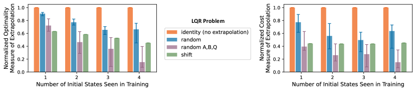
Figure 5: In underdetermined LQR problems (Section 3.2), the extent to which linear controllers learned via policy gradient extrapolate to initial states unseen in training, depends on the degree of exploration that the system induces from initial states that were seen in training. This figure supplements Figure 2 by including results for analogous experiments over an LQR problem with random ${\mathbf{A}}\in{\mathbb{R}}^{D\times D}$, ${\mathbf{B}}\in{\mathbb{R}}^{D\times D}$, and positive semidefinite ${\mathbf{Q}}\in{\mathbb{R}}^{D\times D}$ (instead of just a random ${\mathbf{A}}$). Specifically, in the “random ${\mathbf{A}},{\mathbf{B}},{\mathbf{Q}}$” system, the entries of ${\mathbf{A}}$ and ${\mathbf{B}}$ were sampled independently from a zero-mean Gaussian with standard deviation $1/\sqrt{D}$. As for ${\mathbf{Q}}$, we first sampled the entries of a matrix ${\mathbf{Z}}\in{\mathbb{R}}^{D\times D}$ independently, again from a zero-mean Gaussian with standard deviation $1/\sqrt{D}$. Then, we set ${\mathbf{Q}}={\mathbf{Z}}{\mathbf{Z}}^{\top}$. Results: Non-trivial extrapolation is achieved under the “random ${\mathbf{A}},{\mathbf{B}},{\mathbf{Q}}$” system, in accordance with the fact that random systems generically induce exploration (see discussion in Section 4.4). The extent of extrapolation is significantly better compared to systems where just ${\mathbf{A}}$ is random (referred to as “random” in the legend and analyzed in Theorem 1). Theoretical investigation of this phenomenon is left for future work.

System. In all experiments, except for those with the “random ${\mathbf{A}},{\mathbf{B}},{\mathbf{Q}}$” system (Figure 5), we set ${\mathbf{B}}={\mathbf{Q}}={\mathbf{I}}\in{\mathbb{R}}^{D\times D}$.

Initial states. We took the set of initial states seen in training to be the first $d\in[4]$ standard basis vectors, and used the remaining standard basis vectors for evaluating extrapolation.

Optimization. We ran policy gradient over a linear controller for $10^{5}$ iterations using a learning rate of $10^{-3}$. In the experiments of Figure 2, for all system types, median training cost across random seeds was within $10^{-8}$ of the minimal possible training cost. In the experiments of Figure 4, for all system types with $H=8$, median training cost was within $2\cdot 10^{-5}$ of the minimal possible training cost. Lastly, in the experiments of Figure 5, for the “random ${\mathbf{A}},{\mathbf{B}},{\mathbf{Q}}$” system type, median training cost was within $0.02$ of the minimal possible training cost.

E.3.2 The Pendulum Control Problem (Section 5.2)

System. The two-dimensional state of the system is described by the vertical angle of the pendulum $\theta\in{\mathbb{R}}$ and its angular velocity $\dot{\theta}\in{\mathbb{R}}$. At time step $h$, the controller applies a torque $u_{h}\in{\mathbb{R}}$, giving rise to the following non-linear dynamics for a unit length pendulum with a unit mass object mounted on top of it:

$$\begin{split}\theta_{h}&=\theta_{h-1}+\Delta\cdot\dot{\theta}_{h-1}\\ \dot{\theta}_{h}&=\dot{\theta}_{h-1}+\Delta\cdot\brk 1{u_{h-1}-g\cdot\sin(\theta_{h-1})}\end{split}~{}~{},~{}\forall h\in[H]\text{\,,}$$ (40)

where $\Delta=0.05$ is a time discretization resolution and $g=10$ is the gravitational acceleration constant.

Cost. The goal of the controller is to make the pendulum reach and stay at the target state $(\pi,0)$. Accordingly, the cost at each time step is the squared Euclidean distance from $(\pi,0)$. Specifically, suppose that we are given a (finite) set of initial states ${\mathcal{X}}\subset{\mathbb{R}}^{2}$. For a (state-feedback) controller $\pi_{\mathbf{w}}:{\mathbb{R}}^{2}\to{\mathbb{R}}$, parameterized by ${\mathbf{w}}\in{\mathbb{R}}^{P}$, the cost is defined by:

$$J({\mathbf{w}};{\mathcal{X}}):=\frac{1}{H\cdot\abs{{\mathcal{X}}}}\sum\nolimits_{(\theta_{0},\dot{\theta}_{0})\in{\mathcal{X}}}\sum\nolimits_{h=0}^{H}\norm*{(\theta_{h},\dot{\theta}_{h})-(\pi,0)}^{2}\text{\,,}$$ (41)

where $\theta_{h}$ and $\dot{\theta}_{h}$ evolve according to Equation 40 with $u_{h-1}=\pi_{\mathbf{w}}(\theta_{h-1},\dot{\theta}_{h-1})$, for $h\in[H]$. In all experiments, the time horizon is set to $H=100$.

Initial states. For the experiments of Figure 3, Table 1 specifies the initial states used for training and those used for evaluating extrapolation to initial states unseen in training.

Controller parameterization. We parameterized the controller as a fully-connected neural network with ReLU activation. The network was of depth $4$ and width $50$. Parameters were randomly initialized according to the default PyTorch implementation.

Non-extrapolating controller. To obtain a non-extrapolating controller for Figure 3, we trained the controller using a modified objective instead of the standard training cost. In addition to the cost over initial states seen in training, the modified objective includes an “adversarial” cost term over initial states unseen in training, for which the target state is set to be either $(0,0)$ or $(2\pi,0)$ (as opposed to the original target state $(\pi,0)$). Specifically, for a coefficient $\lambda=0.1$, the modified objective is given by:

$$J({\mathbf{w}};{\mathcal{S}})+\lambda\cdot\frac{1}{H\cdot\abs{{\mathcal{U}}}}\sum\nolimits_{(\theta_{0},\dot{\theta}_{0})\in{\mathcal{U}}}\sum\nolimits_{h=0}^{H}\norm*{(\theta_{h},\dot{\theta}_{h})-\brk*{\bar{\theta}_{\theta_{0}},0}}^{2}\text{\,,}$$

where ${\mathcal{S}}\subset{\mathbb{R}}^{2}$ is the set of initial states seen in training, ${\mathcal{U}}\subset{\mathbb{R}}^{2}\setminus{\mathcal{S}}$ is the set of initial states used for evaluating extrapolation to initial states unseen in training, $J(\cdot\,;{\mathcal{S}})$ is defined by Equation 41, $\theta_{h}$ and $\dot{\theta}_{h}$ evolve according to Equation 40 with $u_{h-1}=\pi_{\mathbf{w}}(\theta_{h-1},\dot{\theta}_{h-1})$, for $h\in[H]$, and $\bar{\theta}_{\theta_{0}}=0$ if $\theta_{0}\leq\pi$ and $\bar{\theta}_{\theta_{0}}=2\pi$ if $\theta_{0}>\pi$. We trained five controllers with this modified objective, using different random seeds, and selected for Figure 3 the one attaining the lowest training cost.

Optimization. The training cost was minimized via policy gradient with learning rate $5\cdot 10^{-4}$. For training the non-extrapolating controller over the modified objective (specified above), we found the Adam optimizer (Kingma & Ba, 2015) to be substantially more effective. Hence, for that purpose, we used Adam with default $\beta_{1},\beta_{2}$ coefficients and learning rate $3\cdot 10^{-4}$. Optimization proceeded until the training objective did not improve by at least $10^{-5}$ over $5,\!000$ consecutive iterations or $75,\!000$ iterations elapsed. The final controller in each run was taken to be that which achieved the lowest training cost across the iterations.

Computing the normalized cost measure of extrapolation. Let ${\mathbf{w}}_{\mathrm{no-ext}}\in{\mathbb{R}}^{P}$ be the parameters of the non-extrapolating controller. The normalized cost measure of extrapolation attained by ${\mathbf{w}}\in{\mathbb{R}}^{P}$ for a set of initial states unseen in training ${\mathcal{U}}\subset{\mathbb{R}}^{2}\setminus{\mathcal{S}}$ is computed as follows: $(J({\mathbf{w}};{\mathcal{U}})-\tilde{J}^{*}({\mathcal{U}}))/(J({\mathbf{w}}_{\mathrm{no-ext}};{\mathcal{U}})-\tilde{J}^{*}({\mathcal{U}}))$, where $J(\cdot\,;{\mathcal{U}})$ is defined by Equation 41 and $\tilde{J}^{*}({\mathcal{U}})$ is an estimate of the minimal possible cost over ${\mathcal{U}}$. We obtained the estimate $\tilde{J}^{*}({\mathcal{U}})$ by training a neural network controller (of the same architecture specified above) for minimizing the cost only over ${\mathcal{U}}$, i.e. for minimizing $J(\cdot\,;{\mathcal{U}})$. We carried out five such runs, differing in random seed, and took $\tilde{J}^{*}({\mathcal{U}})$ to be the minimal cost attained across the runs.

E.3.3 The Quadcopter Control Problem (Section 5.2)

System. The state of the system ${\mathbf{x}}=(x,y,z,\phi,\theta,\psi,\dot{x},\dot{y},\dot{z},\dot{\phi},\dot{\theta},\dot{\psi})\in{\mathbb{R}}^{12}$ comprises the quadcopter’s position $(x,y,z)\in{\mathbb{R}}^{3}$, tilt angles $(\phi,\theta,\psi)\in{\mathbb{R}}^{3}$ (i.e. roll, pitch, and yaw), and their respective velocities. At time step $h$, the controller chooses ${\mathbf{u}}_{h}\in[0,\text{MAX\_RPM}]^{4}$, which determines the revolutions per minute (RPM) for each of the four motors, where $\text{MAX\_RPM}=21713.71$ is the maximal supported RPM. Our implementation of the state dynamics is adapted from the torchcontrol GitHub repository, which is based on the explicit dynamics given in Panerati et al. (2021). For completeness, we lay out explicitly the evolution at time step $h\in[H]$:

$$\begin{split}\begin{pmatrix}x_{h}\\ y_{h}\\ z_{h}\end{pmatrix}&=\begin{pmatrix}x_{h-1}\\ y_{h-1}\\ z_{h-1}\end{pmatrix}+\Delta\cdot\begin{pmatrix}\dot{x}_{h-1}\\ \dot{y}_{h-1}\\ \dot{z}_{h-1}\end{pmatrix}\\[3.99994pt] \begin{pmatrix}\phi_{h}\\ \theta_{h}\\ \psi_{h}\end{pmatrix}&=\begin{pmatrix}\phi_{h-1}\\ \theta_{h-1}\\ \psi_{h-1}\end{pmatrix}+\Delta\cdot\begin{pmatrix}\dot{\phi}_{h-1}\\ \dot{\theta}_{h-1}\\ \dot{\psi}_{h-1}\end{pmatrix}\\[3.99994pt] \begin{pmatrix}\dot{x}_{h}\\ \dot{y}_{h}\\ \dot{z}_{h}\end{pmatrix}&=\begin{pmatrix}\dot{x}_{h-1}\\ \dot{y}_{h-1}\\ \dot{z}_{h-1}\end{pmatrix}+\frac{\Delta}{m}\cdot\brk*{{\mathbf{V}}_{h-1}\begin{pmatrix}0\\ 0\\ k_{f}\cdot\norm{{\mathbf{u}}_{h-1}}^{2}\end{pmatrix}-\begin{pmatrix}0\\ 0\\ g\end{pmatrix}}\\[3.99994pt] \begin{pmatrix}\dot{\phi}_{h}\\ \dot{\theta}_{h}\\ \dot{\psi}_{h}\end{pmatrix}&=\begin{pmatrix}\dot{\phi}_{h-1}\\ \dot{\theta}_{h-1}\\ \dot{\psi}_{h-1}\end{pmatrix}+\Delta\cdot{\mathbf{P}}^{-1}\brk*{\begin{pmatrix}\frac{k_{F}\cdot l}{\sqrt{2}}\cdot\brk{{\mathbf{u}}^{2}_{h-1}[1]+{\mathbf{u}}^{2}_{h-1}[2]-{\mathbf{u}}^{2}_{h-1}[3]-{\mathbf{u}}^{2}_{h-1}[4]}\\ \frac{k_{F}\cdot l}{\sqrt{2}}\cdot\brk{-{\mathbf{u}}^{2}_{h-1}[1]+{\mathbf{u}}^{2}_{h-1}[2]+{\mathbf{u}}^{2}_{h-1}[3]-{\mathbf{u}}^{2}_{h-1}[4]}\\ k_{T}\cdot\brk{-{\mathbf{u}}^{2}_{h-1}[1]+{\mathbf{u}}^{2}_{h-1}[2]-{\mathbf{u}}^{2}_{h-1}[3]+{\mathbf{u}}^{2}_{h-1}[4]}\end{pmatrix}-\begin{pmatrix}\dot{\phi}_{h-1}\\ \dot{\theta}_{h-1}\\ \dot{\psi}_{h-1}\end{pmatrix}\times{\mathbf{P}}\begin{pmatrix}\dot{\phi}_{h-1}\\ \dot{\theta}_{h-1}\\ \dot{\psi}_{h-1}\end{pmatrix}}\end{split}\text{\,,}$$ (42)

where $\times$ stands here for the cross product of two vectors, ${\mathbf{u}}_{h-1}[1],\ldots,{\mathbf{u}}_{h-1}[4]$ are the entries of ${\mathbf{u}}_{h-1}$, $\Delta=0.02$ is the time discretization resolution, $g=9.81$ is the gravitational acceleration constant, $m=0.027$ is the quadcopter’s mass, $l=0.0397$ is the quadcopter’s arm length, $k_{F}=3.16\cdot 10^{-10},K_{T}=7.94\cdot 10^{-12}$ describe physical constants related to the conversion of motor RPM to torque, and:

$$\begin{split}{\mathbf{V}}_{h-1}&=\begin{pmatrix}\cos(\theta)&\sin(\theta)\sin(\phi)&\sin(\theta)\cos(\phi)\\ \sin(\theta)\sin(\psi)&-\cos(\theta)\sin(\phi)\sin(\psi)+\cos(\phi)\cos(\psi)&-\cos(\theta)\cos(\phi)\sin(\psi)-\sin(\phi)\cos(\psi)\\ -\sin(\theta)\cos(\psi)&\cos(\theta)\sin(\phi)\cos(\psi)+J(\phi)\sin(\psi)&\cos(\theta)\cos(\phi)\cos(\psi)-\sin(\phi)\sin(\psi)\end{pmatrix}\\[3.99994pt] {\mathbf{P}}&=\begin{pmatrix}1.4\cdot 10^{-5}&0&0\\ 0&1.4\cdot 10^{-5}&0\\ 0&0&2.17\cdot 10^{-5}\end{pmatrix}\end{split}$$

are rotation and inertial matrices, respectively. For brevity of notation, we omitted the subscript $h-1$ from $\phi,\theta,\psi$ in the definition of ${\mathbf{V}}_{h-1}$.

Cost. The goal of the controller is to make the quadcopter reach and stay at the target state ${\mathbf{x}}^{*}=(0,0,1,0,\ldots,0)$. In accordance with the torchcontrol implementation, the cost at each time step is a weighted squared Euclidean distance from ${\mathbf{x}}^{*}$. Specifically, suppose that we are given a (finite) set of initial states ${\mathcal{X}}\subset{\mathbb{R}}^{12}$. For a (state-feedback) controller $\pi_{\mathbf{w}}:{\mathbb{R}}^{12}\to[0,\text{MAX\_RPM}]^{4}$, parameterized by ${\mathbf{w}}\in{\mathbb{R}}^{P}$, the cost is defined by:

$$J({\mathbf{w}};{\mathcal{X}}):=\frac{1}{H\cdot\abs{{\mathcal{X}}}}\sum\nolimits_{{\mathbf{x}}_{0}\in{\mathcal{X}}}\sum\nolimits_{h=0}^{H}\sum\nolimits_{d=1}^{12}\alpha_{d}^{2}\cdot\brk*{{\mathbf{x}}_{h}[d]-{\mathbf{x}}^{*}[d]}^{2}\text{\,,}$$ (43)

where ${\mathbf{x}}_{h}\in{\mathbb{R}}^{12}$ evolves according to Equation 42 with ${\mathbf{u}}_{h-1}=\pi_{\mathbf{w}}({\mathbf{x}}_{h-1})$, for $h\in[H]$, the cost weights are $\alpha_{1}=\alpha_{2}=\alpha_{3}=1$ and $\alpha_{4}=\cdots=\alpha_{12}=0.1$, and ${\mathbf{x}}_{h}[d],{\mathbf{x}}^{*}[d]$ denote the $d$’th entries of ${\mathbf{x}}_{h},{\mathbf{x}}^{*}$, respectively. In all experiments, the time horizon is set to $H=50$.

Initial states. For the experiments of Figures 3, 8, and 10, Tables 2, LABEL:, 3, and 4 specify the initial states used for training and those used for evaluating extrapolation to initial states unseen in training, respectively.

Controller parameterization. As in pendulum control experiments (cf. Section E.3.2), we parameterized the controller as a fully-connected neural network with ReLU activation. The network was of depth $4$ and width $50$, and its parameters were randomly initialized according to the default PyTorch implementation. To convert the network’s outputs into values within $[0,\text{MAX\_RPM}]$, we applied the hyperbolic tangent activation and linearly scaled the result. That is, denoting by ${\mathbf{z}}\in{\mathbb{R}}^{4}$ the output of the network for some state, the chosen control was ${\mathbf{u}}=(\tanh({\mathbf{z}})+{\mathbf{1}})\cdot\frac{\text{MAX\_RPM}}{2}$, where $\tanh$ is applied element-wise and ${\mathbf{1}}\in{\mathbb{R}}^{4}$ is the vector whose entries are all equal to one.

Non-extrapolating controller. Similarly to the pendulum control experiments (cf. Section E.3.2), to obtain a non-extrapolating controller baselines for Figures 3, 8, and 10, we trained controllers using a modified objective instead of the standard training cost. In addition to the cost over initial states seen in training, the modified objective includes an “adversarial” cost term over initial states unseen in training, for which the target state is set to be $\bar{{\mathbf{x}}}=(0,0,0,0,\ldots,0)$ (as opposed to the original target state ${\mathbf{x}}^{*}=(0,0,1,0,\ldots,0)$). Specifically, for a coefficient $\lambda=0.1$, the modified objective is given by:

$$J({\mathbf{w}};{\mathcal{S}})+\lambda\cdot\frac{1}{\abs{H\cdot{\mathcal{U}}}}\sum\nolimits_{{\mathbf{x}}_{0}\in{\mathcal{U}}}\sum\nolimits_{h=0}^{H}\sum\nolimits_{d=1}^{12}\alpha_{d}^{2}\cdot\brk*{{\mathbf{x}}_{h}[d]-\bar{{\mathbf{x}}}[d]}^{2}\text{\,,}$$

where ${\mathcal{S}}\subset{\mathbb{R}}^{12}$ is the set of initial states seen in training, ${\mathcal{U}}\subset{\mathbb{R}}^{12}\setminus{\mathcal{S}}$ is the set of initial states used for evaluating extrapolation to initial states unseen in training, $J(\cdot\,;{\mathcal{S}})$ is defined by Equation 43, ${\mathbf{x}}_{h}\in{\mathbb{R}}^{12}$ evolves according to Equation 42 with ${\mathbf{u}}_{h-1}=\pi_{\mathbf{w}}({\mathbf{x}}_{h-1})$, for $h\in[H]$, the cost weights are $\alpha_{1}=\alpha_{2}=\alpha_{3}=1$ and $\alpha_{4}=\cdots=\alpha_{12}=0.1$, and ${\mathbf{x}}_{h}[d],\bar{{\mathbf{x}}}[d]$ denote the $d$’th entries of ${\mathbf{x}}_{h},\bar{{\mathbf{x}}}$, respectively. For each of Figures 3, 8, and 10, we trained five controllers with this modified objective, using different random seeds, and selected the one attaining the lowest training cost.

Optimization. In all experiments, the training cost was minimized via the Adam optimizer (Kingma & Ba, 2015) with default $\beta_{1},\beta_{2}$ coefficients and learning rate $3\cdot 10^{-4}$. Optimization proceeded until the training objective did not improve by at least $10^{-5}$ over $5,\!000$ consecutive iterations or $75,\!000$ iterations elapsed. The final controller in each run was taken to be that which achieved the lowest training cost across the iterations.

Computing the normalized cost measure of extrapolation. The normalized cost measure of extrapolation was computed according to the process described in Section E.3.2 for the pendulum control experiments.

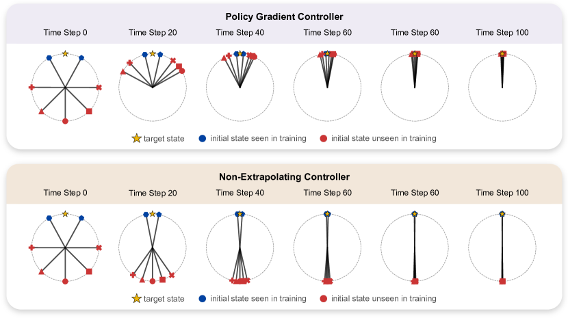
Figure 6: For the pendulum control experiments in Figure 3, presented is the evolution of states through time under the policy gradient (top) and non-extrapolating (bottom) controllers.

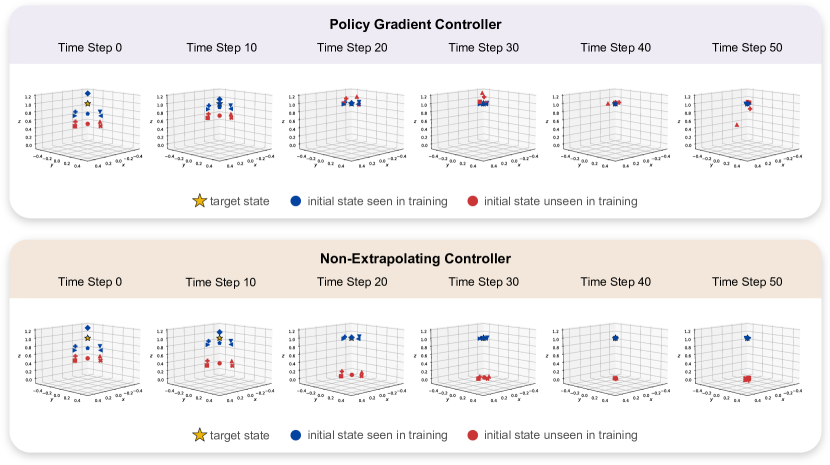
Figure 7: For the quadcopter control experiments in Figure 3, presented is the evolution of states through time under the policy gradient (top) and non-extrapolating (bottom) controllers.

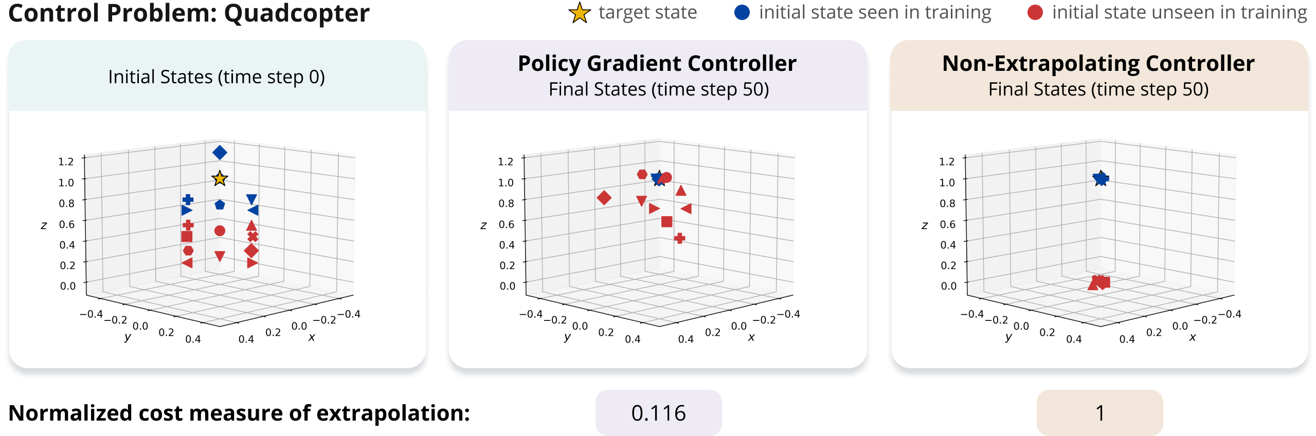
Figure 8: In the quadcopter control problem (Section 5.2), a (non-linear) neural network controller trained via policy gradient often extrapolates to initial states unseen in training, despite the existence of non-extrapolating controllers. This figure supplements Figure 3 by including the results of an identical experiment, but with additional unseen initial states that are farther away from the initial states seen in training. See caption of Figure 3 for details on the experiment. Results: As one might expect, while the extent of extrapolation is still highly non-trivial, it decays the farther away initial states unseen in training are from the initial states seen in training. Further details in Appendix E: Table 3 fully specifies the initial and final states depicted above, and Figure 9 presents the evolution of states through time under the policy gradient and non-extrapolating controllers.

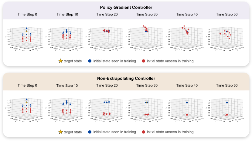
Figure 9: For the policy gradient (top) and non-extrapolating (bottom) controllers from Figure 8, presented is the evolution of states through time.

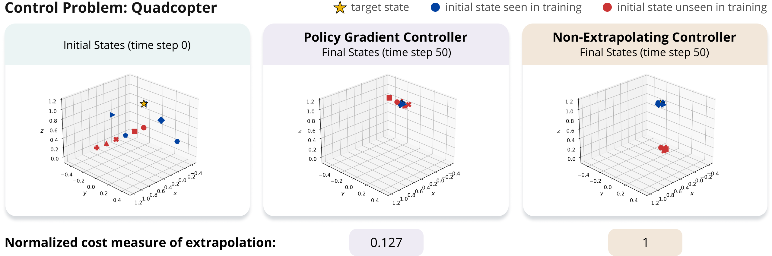
Figure 10: In the quadcopter control problem (Section 5.2), a (non-linear) neural network controller trained via policy gradient often extrapolates to initial states unseen in training (at different horizontal distances from the target state), despite the existence of non-extrapolating controllers. This figure supplements Figure 3 by including the results of an analogous experiment, where the unseen initial states are at different horizontal distances from the initial states seen in training (instead of being at a lower height). See caption of Figure 3 for details on the experiment. Results: Remarkably, the controller trained via policy gradient extrapolates well to unseen initial states at various horizontal distances from the initial states seen in training. In contrast to unseen initial states below those used for training, for which extrapolation was observed in Figure 3, an uncontrolled system does not induce exploration to states at different horizontal distances, in the naive sense of visiting the state along trajectories emanating from the initial states seen in training. Hence, the results of this experiment highlight the importance of finding a quantitative measure of exploration for non-linear systems, which may facilitate the theoretical study of extrapolation therein. Further details in Appendix E: Table 4 fully specifies the initial and final states depicted above, and Figure 11 presents the evolution of states through time under the policy gradient and non-extrapolating controllers.

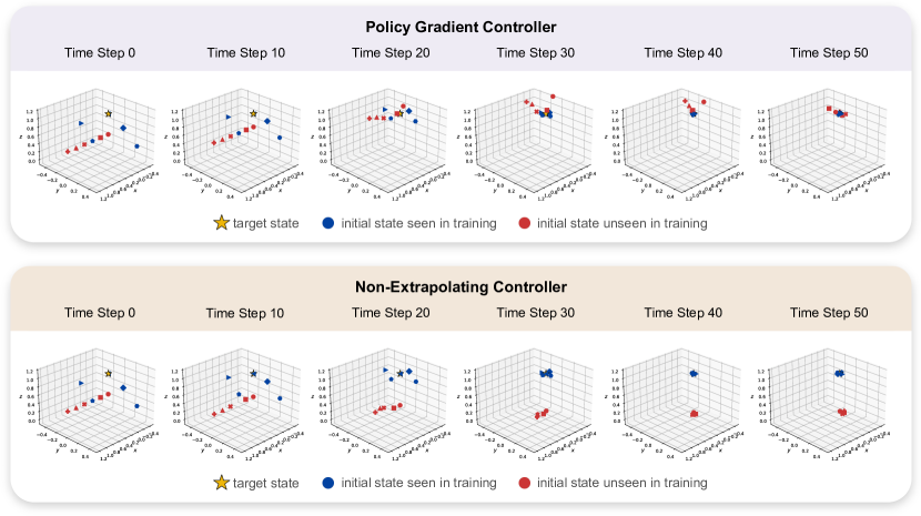
Figure 11: For the policy gradient (top) and non-extrapolating (bottom) controllers from Figure 10, presented is the evolution of states through time.

Table 1: Target, initial, and final states for the pendulum control experiments depicted in Figure 3. Each state is described by the vertical angle of the pendulum $\theta\in{\mathbb{R}}$ and its angular velocity $\dot{\theta}\in{\mathbb{R}}$.

		$\theta$	$\dot{\theta}$
	Target State	3.14	0
Training	Initial States	2.64	0.00
		3.64	0.00
	Final States for Policy Gradient Controller	3.13	0.01
		3.15	-0.01
	Final States for Non-Extrapolating Controller	3.14	0.00
		3.15	-0.00
Unseen	Initial States	0.00	0.00
		0.79	0.00
		1.57	0.00
		4.71	0.00
		5.50	0.00
	Final States for Policy Gradient Controller	3.10	0.03
		3.10	0.03
		3.11	0.02
		3.17	-0.03
		3.18	-0.04
	Final States for Non-Extrapolating Controller	-0.00	-0.00
		0.01	-0.00
		0.02	-0.01
		6.27	0.01
		6.28	0.01

Table 2: Target, initial, and final states for the quadcopter control experiments depicted in Figure 3. Each state of the system ${\mathbf{x}}=(x,y,z,\phi,\theta,\psi,\dot{x},\dot{y},\dot{z},\dot{\phi},\dot{\theta},\dot{\psi})\in{\mathbb{R}}^{12}$ comprises the quadcopter’s position $(x,y,z)$, tilt angles $(\phi,\theta,\psi)$ (i.e. roll, pitch, and yaw), and their respective velocities.

		$x$	$y$	$z$	$\phi$	$\theta$	$\psi$	$\dot{x}$	$\dot{y}$	$\dot{z}$	$\dot{\phi}$	$\dot{\theta}$	$\dot{\psi}$
	Target State	0	0	1	0	0	0	0	0	0	0	0	0
Training	Initial States	0.00	0.00	0.75	0.00	0.00	0.00	0.00	0.00	0.00	0.00	0.00	0.00
		0.00	0.00	1.00	0.00	0.00	0.00	0.00	0.00	0.00	0.00	0.00	0.00
		0.00	0.00	1.25	0.00	0.00	0.00	0.00	0.00	0.00	0.00	0.00	0.00
		0.25	0.00	0.75	0.00	0.00	0.00	0.00	0.00	0.00	0.00	0.00	0.00
		0.00	0.25	0.75	0.00	0.00	0.00	0.00	0.00	0.00	0.00	0.00	0.00
		-0.25	0.00	0.75	0.00	0.00	0.00	0.00	0.00	0.00	0.00	0.00	0.00
		0.00	-0.25	0.75	0.00	0.00	0.00	0.00	0.00	0.00	0.00	0.00	0.00
	Final States for Policy Gradient Controller	0.00	-0.00	1.00	-0.01	-0.00	0.01	-0.01	0.00	0.00	0.00	0.00	0.02
		0.00	0.00	1.00	-0.01	-0.00	0.01	0.00	-0.00	-0.01	-0.01	0.00	0.01
		-0.00	0.00	1.00	-0.01	0.00	0.01	0.00	-0.00	-0.01	-0.01	-0.00	0.01
		-0.03	-0.00	1.00	-0.01	0.07	0.01	-0.10	-0.00	-0.01	-0.02	-0.11	0.01
		-0.00	-0.02	1.00	-0.05	-0.00	-0.02	0.00	0.02	0.02	0.11	0.02	0.15
		0.03	0.00	1.00	-0.01	-0.07	0.01	0.10	0.01	-0.00	-0.00	0.09	0.02
		-0.00	0.02	1.00	0.03	-0.00	0.04	0.01	-0.01	-0.06	-0.12	-0.02	-0.12
	Final States for Non-Extrapolating Controller	0.00	-0.00	1.00	0.02	0.00	-0.02	0.00	0.01	0.01	0.02	0.00	-0.01
		0.00	-0.00	1.00	0.02	0.00	-0.02	0.01	0.01	0.01	0.02	-0.00	-0.01
		-0.00	-0.00	1.00	0.01	0.00	-0.01	0.01	-0.01	-0.00	0.00	-0.01	-0.03
		-0.03	0.00	1.00	0.03	0.09	-0.04	-0.09	0.00	-0.02	0.04	-0.12	-0.05
		-0.00	-0.02	1.00	-0.01	0.00	-0.06	-0.02	0.05	0.00	0.20	0.05	0.15
		0.03	0.00	1.01	0.00	-0.08	0.01	0.09	0.00	0.02	-0.00	0.12	0.04
		0.00	0.02	1.01	0.05	0.00	0.02	0.02	-0.04	-0.00	-0.17	-0.06	-0.18
Unseen	Initial States	0.00	0.00	0.50	0.00	0.00	0.00	0.00	0.00	0.00	0.00	0.00	0.00
		0.25	0.00	0.50	0.00	0.00	0.00	0.00	0.00	0.00	0.00	0.00	0.00
		0.00	0.25	0.50	0.00	0.00	0.00	0.00	0.00	0.00	0.00	0.00	0.00
		-0.25	0.00	0.50	0.00	0.00	0.00	0.00	0.00	0.00	0.00	0.00	0.00
		0.00	-0.25	0.50	0.00	0.00	0.00	0.00	0.00	0.00	0.00	0.00	0.00
	Final States for Policy Gradient Controller	-0.00	-0.00	1.00	-0.01	0.00	0.00	0.00	0.01	0.01	-0.00	-0.01	0.02
		-0.03	0.01	1.02	0.01	0.07	0.01	-0.08	0.02	-0.03	0.04	-0.12	0.05
		-0.01	-0.00	1.04	-0.02	-0.00	0.00	0.05	0.07	-0.06	0.12	-0.08	0.16
		0.16	-0.05	0.50	-0.07	-0.71	-0.19	-0.12	0.06	-3.19	0.70	4.80	-0.25
		-0.01	0.05	0.88	0.06	-0.01	0.03	-0.02	-0.38	-0.05	-0.68	0.93	-0.44
	Final States for Non-Extrapolating Controller	0.02	0.01	-0.01	0.09	0.02	-0.11	0.14	0.05	0.03	0.17	-0.03	-0.15
		-0.03	0.01	0.00	0.10	0.13	-0.11	-0.10	0.02	-0.39	0.02	0.15	0.33
		0.02	-0.02	0.00	0.03	0.02	-0.16	0.08	0.05	0.04	0.38	-0.03	0.06
		0.06	0.02	-0.02	0.06	-0.09	-0.06	0.31	0.07	-0.09	0.13	-0.06	-0.10
		0.02	0.04	-0.04	0.15	0.02	-0.02	0.11	0.10	-0.57	-0.17	0.04	0.08

Table 3: Target, initial, and final states for the quadcopter control experiments depicted in Figure 8. Each state of the system ${\mathbf{x}}=(x,y,z,\phi,\theta,\psi,\dot{x},\dot{y},\dot{z},\dot{\phi},\dot{\theta},\dot{\psi})\in{\mathbb{R}}^{12}$ comprises the quadcopter’s position $(x,y,z)$, tilt angles $(\phi,\theta,\psi)$ (i.e. roll, pitch, and yaw), and their respective velocities.

		$x$	$y$	$z$	$\phi$	$\theta$	$\psi$	$\dot{x}$	$\dot{y}$	$\dot{z}$	$\dot{\phi}$	$\dot{\theta}$	$\dot{\psi}$
	Target State	0	0	1	0	0	0	0	0	0	0	0	0
Training	Initial States	0.00	0.00	0.75	0.00	0.00	0.00	0.00	0.00	0.00	0.00	0.00	0.00
		0.00	0.00	1.00	0.00	0.00	0.00	0.00	0.00	0.00	0.00	0.00	0.00
		0.00	0.00	1.25	0.00	0.00	0.00	0.00	0.00	0.00	0.00	0.00	0.00
		0.25	0.00	0.75	0.00	0.00	0.00	0.00	0.00	0.00	0.00	0.00	0.00
		0.00	0.25	0.75	0.00	0.00	0.00	0.00	0.00	0.00	0.00	0.00	0.00
		-0.25	0.00	0.75	0.00	0.00	0.00	0.00	0.00	0.00	0.00	0.00	0.00
		0.00	-0.25	0.75	0.00	0.00	0.00	0.00	0.00	0.00	0.00	0.00	0.00
	Final States for Policy Gradient Controller	-0.00	0.00	1.00	0.01	0.00	-0.00	-0.01	0.01	-0.00	0.02	0.02	-0.00
		0.00	0.00	1.00	0.01	-0.00	-0.01	-0.00	-0.01	0.00	0.00	0.01	-0.01
		0.00	-0.00	1.00	0.01	-0.00	-0.02	0.00	-0.01	-0.00	-0.00	-0.00	-0.02
		-0.02	0.00	1.00	0.04	0.09	-0.04	-0.04	0.01	-0.02	0.09	-0.11	0.04
		-0.00	-0.02	1.00	-0.01	0.00	-0.07	0.01	0.03	0.01	0.21	-0.01	0.16
		0.03	-0.00	1.00	0.02	-0.09	-0.01	0.05	-0.02	0.01	-0.06	0.08	-0.03
		0.00	0.02	1.00	0.03	-0.00	0.04	0.01	-0.05	0.02	-0.17	-0.02	-0.18
	Final States for Non-Extrapolating Controller	-0.00	0.00	1.00	0.02	-0.00	-0.02	0.01	0.03	0.01	0.04	-0.01	-0.00
		-0.00	0.00	1.00	0.02	-0.00	-0.02	-0.00	0.02	0.00	0.03	0.00	-0.01
		-0.00	0.00	1.00	0.02	0.00	-0.02	-0.01	0.03	0.00	0.04	0.02	-0.01
		-0.03	-0.00	1.00	0.02	0.10	-0.01	-0.03	-0.02	-0.03	-0.02	-0.16	-0.01
		-0.00	-0.02	1.01	-0.01	-0.01	-0.07	-0.02	0.07	0.06	0.22	0.01	0.12
		0.03	0.01	1.00	0.02	-0.10	-0.04	0.05	0.05	0.04	0.03	0.08	-0.03
		-0.00	0.02	1.00	0.04	0.01	0.03	0.01	-0.04	-0.05	-0.17	-0.00	-0.15
Unseen	Initial States	0.00	0.00	0.50	0.00	0.00	0.00	0.00	0.00	0.00	0.00	0.00	0.00
		0.25	0.00	0.50	0.00	0.00	0.00	0.00	0.00	0.00	0.00	0.00	0.00
		0.00	0.25	0.50	0.00	0.00	0.00	0.00	0.00	0.00	0.00	0.00	0.00
		-0.25	0.00	0.50	0.00	0.00	0.00	0.00	0.00	0.00	0.00	0.00	0.00
		0.00	-0.25	0.50	0.00	0.00	0.00	0.00	0.00	0.00	0.00	0.00	0.00
		0.00	0.00	0.25	0.00	0.00	0.00	0.00	0.00	0.00	0.00	0.00	0.00
		0.25	0.00	0.25	0.00	0.00	0.00	0.00	0.00	0.00	0.00	0.00	0.00
		0.00	0.25	0.25	0.00	0.00	0.00	0.00	0.00	0.00	0.00	0.00	0.00
		-0.25	0.00	0.25	0.00	0.00	0.00	0.00	0.00	0.00	0.00	0.00	0.00
		0.00	-0.25	0.25	0.00	0.00	0.00	0.00	0.00	0.00	0.00	0.00	0.00
	Final States for Policy Gradient Controller	-0.01	0.05	1.02	0.01	0.02	0.03	-0.27	0.07	0.02	0.09	0.55	0.01
		0.09	0.14	0.64	0.07	0.46	0.23	1.51	0.47	0.00	1.23	-2.99	0.81
		0.01	0.02	1.01	-0.00	-0.00	-0.04	-0.15	0.00	0.00	0.15	0.23	0.09
		-0.04	0.13	0.91	0.02	0.16	0.15	-0.77	0.21	-0.03	0.10	2.32	0.15
		0.10	0.25	0.51	-0.10	0.27	0.58	0.21	0.02	-1.40	1.27	2.83	0.84
		0.24	0.11	0.85	-0.57	-0.54	0.28	0.17	0.35	-2.93	1.37	-0.08	2.25
		-0.14	0.07	0.70	-0.73	0.84	0.03	-0.10	0.59	-3.11	1.00	2.67	1.19
		0.09	0.05	0.74	-0.33	0.11	0.06	-0.15	0.66	-1.42	1.01	3.72	0.83
		0.55	0.14	0.95	-1.13	-1.16	0.17	0.89	0.52	-3.04	1.43	-0.90	3.42
		0.35	0.22	1.14	-0.74	-0.48	0.34	0.41	0.74	-2.68	0.18	-1.60	2.29
	Final States for Non-Extrapolating Controller	-0.01	-0.02	0.01	-0.00	0.01	0.01	-0.00	-0.10	0.00	-0.24	0.03	0.01
		-0.04	-0.01	-0.01	0.04	0.17	-0.02	-0.01	-0.05	-0.09	-0.01	-0.39	0.01
		0.00	-0.03	0.01	-0.03	-0.01	-0.05	-0.03	0.05	-0.02	0.32	-0.03	0.16
		0.04	-0.02	-0.02	-0.02	-0.16	-0.00	-0.09	-0.06	0.08	-0.03	0.67	-0.16
		0.00	0.02	-0.01	0.05	0.01	0.06	-0.06	-0.14	-0.13	-0.27	0.08	-0.25
		-0.01	-0.03	-0.00	0.00	0.01	-0.01	-0.01	-0.04	0.02	-0.13	-0.00	0.03
		-0.02	-0.01	-0.01	0.03	0.13	-0.02	0.03	-0.06	-0.11	-0.08	-0.42	0.08
		0.00	-0.02	0.00	-0.03	-0.02	-0.05	0.02	0.02	0.04	0.19	-0.17	0.24
		-0.02	-0.00	-0.01	-0.01	-0.08	0.00	-0.08	-0.05	0.03	0.05	0.35	-0.13
		-0.00	0.01	-0.01	0.05	0.01	0.05	0.01	-0.10	-0.16	-0.17	-0.03	-0.23

Table 4: Target, initial, and final states for the quadcopter control experiments depicted in Figure 10. Each state of the system ${\mathbf{x}}=(x,y,z,\phi,\theta,\psi,\dot{x},\dot{y},\dot{z},\dot{\phi},\dot{\theta},\dot{\psi})\in{\mathbb{R}}^{12}$ comprises the quadcopter’s position $(x,y,z)$, tilt angles $(\phi,\theta,\psi)$ (i.e. roll, pitch, and yaw), and their respective velocities.

		$x$	$y$	$z$	$\phi$	$\theta$	$\psi$	$\dot{x}$	$\dot{y}$	$\dot{z}$	$\dot{\phi}$	$\dot{\theta}$	$\dot{\psi}$
	Target State	0	0	1	0	0	0	0	0	0	0	0	0
Training	Initial States	0.50	0.00	0.50	0.00	0.00	0.00	0.00	0.00	0.00	0.00	0.00	0.00
		0.00	0.50	0.50	0.00	0.00	0.00	0.00	0.00	0.00	0.00	0.00	0.00
		-0.50	0.00	0.50	0.00	0.00	0.00	0.00	0.00	0.00	0.00	0.00	0.00
		0.00	-0.50	0.50	0.00	0.00	0.00	0.00	0.00	0.00	0.00	0.00	0.00
		0.00	0.00	1.00	0.00	0.00	0.00	0.00	0.00	0.00	0.00	0.00	0.00
	Final States for Policy Gradient Controller	-0.05	-0.02	1.00	-0.02	0.25	0.01	0.03	-0.06	-0.11	-0.02	-0.05	0.00
		-0.01	-0.03	0.99	-0.14	0.01	-0.13	-0.04	0.27	-0.07	0.14	0.06	0.10
		0.04	0.00	1.01	0.00	-0.25	-0.03	-0.09	0.04	-0.01	0.12	0.12	0.14
		-0.01	0.03	1.01	0.17	0.01	0.13	0.00	-0.32	0.06	-0.09	-0.04	-0.19
		0.00	-0.00	1.00	0.01	0.00	-0.01	0.01	0.00	-0.01	0.01	-0.01	-0.01
	Final States for Non-Extrapolating Controller	-0.06	-0.00	1.01	-0.04	0.20	0.02	-0.03	-0.03	-0.06	-0.06	-0.25	-0.07
		0.01	-0.04	1.01	-0.13	0.02	-0.09	0.02	0.19	-0.08	0.31	0.04	0.21
		0.06	-0.00	1.01	0.04	-0.20	-0.02	-0.02	0.02	0.15	0.09	0.42	0.08
		-0.01	0.04	1.00	0.15	-0.01	0.09	-0.05	-0.24	-0.28	-0.12	0.05	-0.46
		-0.00	-0.00	1.00	0.03	-0.00	-0.02	-0.02	-0.02	0.04	-0.08	0.01	-0.07
Unseen	Initial States	0.00	0.00	0.50	0.00	0.00	0.00	0.00	0.00	0.00	0.00	0.00	0.00
		0.25	0.00	0.50	0.00	0.00	0.00	0.00	0.00	0.00	0.00	0.00	0.00
		0.75	0.00	0.50	0.00	0.00	0.00	0.00	0.00	0.00	0.00	0.00	0.00
		1.00	0.00	0.50	0.00	0.00	0.00	0.00	0.00	0.00	0.00	0.00	0.00
		1.25	0.00	0.50	0.00	0.00	0.00	0.00	0.00	0.00	0.00	0.00	0.00
	Final States for Policy Gradient Controller	0.15	0.01	1.09	0.38	0.90	0.83	2.30	-2.22	-1.55	1.57	1.17	0.80
		0.10	-0.13	1.09	-0.11	0.08	-0.00	0.71	-0.55	0.01	-0.95	-0.64	-0.77
		-0.10	0.05	0.99	-0.10	0.54	-0.09	0.38	0.77	0.25	0.69	0.10	-0.62
		-0.03	0.03	0.97	-0.32	1.02	-0.23	1.72	1.46	-0.64	-0.12	0.90	-1.17
		-0.11	-0.06	0.98	-0.41	1.20	-0.12	0.92	1.11	-1.42	-0.53	2.14	-1.16
	Final States for Non-Extrapolating Controller	-0.09	-0.04	0.02	-0.01	0.04	-0.06	-0.04	0.03	0.21	-0.12	0.20	-0.24
		-0.13	0.02	0.00	0.01	0.18	0.02	-0.20	-0.05	0.20	-0.00	-0.12	-0.04
		-0.07	0.01	-0.01	-0.01	0.23	0.03	-0.34	0.02	-0.14	0.18	-0.51	-0.24
		-0.11	0.00	0.01	-0.05	0.30	-0.01	-0.18	0.08	-0.11	0.15	-0.81	-0.10
		-0.16	0.00	0.02	-0.11	0.40	0.01	-0.14	0.07	-0.05	0.21	-0.97	-0.29

References

• Abbe et al. (2022) Abbe, E., Bengio, S., Cornacchia, E., Kleinberg, J., Lotfi, A., Raghu, M., and Zhang, C. Learning to reason with neural networks: Generalization, unseen data and boolean measures. Advances in Neural Information Processing Systems, 35, 2022.
• Abbe et al. (2023) Abbe, E., Bengio, S., Lotfi, A., and Rizk, K. Generalization on the unseen, logic reasoning and degree curriculum. In International conference on machine learning. PMLR, 2023.
• Agarwal et al. (2019a) Agarwal, N., Bullins, B., Hazan, E., Kakade, S., and Singh, K. Online control with adversarial disturbances. In International Conference on Machine Learning. PMLR, 2019a.
• Agarwal et al. (2019b) Agarwal, N., Hazan, E., and Singh, K. Logarithmic regret for online control. Advances in Neural Information Processing Systems, 32, 2019b.
• Anderson & Moore (2007) Anderson, B. D. and Moore, J. B. Optimal control: linear quadratic methods. Courier Corporation, 2007.
• Anderson et al. (2010) Anderson, G. W., Guionnet, A., and Zeitouni, O. An introduction to random matrices. Number 118. Cambridge university press, 2010.
• Andriushchenko et al. (2023) Andriushchenko, M., Varre, A. V., Pillaud-Vivien, L., and Flammarion, N. Sgd with large step sizes learns sparse features. In International Conference on Machine Learning. PMLR, 2023.
• Arora et al. (2019) Arora, S., Cohen, N., Hu, W., and Luo, Y. Implicit regularization in deep matrix factorization. In Advances in Neural Information Processing Systems, 2019.
• Azulay et al. (2021) Azulay, S., Moroshko, E., Nacson, M. S., Woodworth, B. E., Srebro, N., Globerson, A., and Soudry, D. On the implicit bias of initialization shape: Beyond infinitesimal mirror descent. In International Conference on Machine Learning, 2021.
• Bhandari & Russo (2019) Bhandari, J. and Russo, D. Global optimality guarantees for policy gradient methods. arXiv preprint arXiv:1906.01786, 2019.
• Bu et al. (2019) Bu, J., Mesbahi, A., Fazel, M., and Mesbahi, M. Lqr through the lens of first order methods: Discrete-time case. arXiv preprint arXiv:1907.08921, 2019.
• Bu et al. (2020) Bu, J., Mesbahi, A., and Mesbahi, M. Policy gradient-based algorithms for continuous-time linear quadratic control. arXiv preprint arXiv:2006.09178, 2020.
• Caron & Traynor (2005) Caron, R. and Traynor, T. The zero set of a polynomial. WSMR Report, pp.  05–02, 2005.
• Cassel & Koren (2021) Cassel, A. B. and Koren, T. Online policy gradient for model free learning of linear quadratic regulators with $\sqrt{T}$ regret. In International Conference on Machine Learning. PMLR, 2021.
• Chen et al. (2023) Chen, X., Minasyan, E., Lee, J. D., and Hazan, E. Regret guarantees for online deep control. In Learning for Dynamics and Control Conference. PMLR, 2023.
• Chou et al. (2023) Chou, H.-H., Maly, J., and Rauhut, H. More is less: inducing sparsity via overparameterization. Information and Inference: A Journal of the IMA, 12(3), 2023.
• Chou et al. (2024) Chou, H.-H., Gieshoff, C., Maly, J., and Rauhut, H. Gradient descent for deep matrix factorization: Dynamics and implicit bias towards low rank. Applied and Computational Harmonic Analysis, 68:101595, 2024.
• Clavera et al. (2020) Clavera, I., Fu, V., and Abbeel, P. Model-augmented actor-critic: Backpropagating through paths. International Conference on Learning Representations, 2020.
• Cohen et al. (2018) Cohen, A., Hasidim, A., Koren, T., Lazic, N., Mansour, Y., and Talwar, K. Online linear quadratic control. In International Conference on Machine Learning. PMLR, 2018.
• Cohen-Karlik et al. (2022) Cohen-Karlik, E., David, A. B., Cohen, N., and Globerson, A. On the implicit bias of gradient descent for temporal extrapolation. In International Conference on Artificial Intelligence and Statistics. PMLR, 2022.
• Cohen-Karlik et al. (2023) Cohen-Karlik, E., Menuhin-Gruman, I., Cohen, N., Giryes, R., and Globerson, A. Learning low dimensional state spaces with overparameterized recurrent neural network. In International Conference on Learning Representations, 2023.
• Dulac-Arnold et al. (2021) Dulac-Arnold, G., Levine, N., Mankowitz, D. J., Li, J., Paduraru, C., Gowal, S., and Hester, T. Challenges of real-world reinforcement learning: definitions, benchmarks and analysis. Machine Learning, 110(9):2419–2468, 2021.
• Fazel et al. (2018) Fazel, M., Ge, R., Kakade, S., and Mesbahi, M. Global convergence of policy gradient methods for the linear quadratic regulator. In International conference on machine learning. PMLR, 2018.
• Frei et al. (2023a) Frei, S., Vardi, G., Bartlett, P., and Srebro, N. Benign overfitting in linear classifiers and leaky relu networks from kkt conditions for margin maximization. In The Thirty Sixth Annual Conference on Learning Theory. PMLR, 2023a.
• Frei et al. (2023b) Frei, S., Vardi, G., Bartlett, P. L., and Srebro, N. The double-edged sword of implicit bias: Generalization vs. robustness in relu networks. Advances in Neural Information Processing Systems, 36, 2023b.
• Fujimoto et al. (2019) Fujimoto, S., Meger, D., and Precup, D. Off-policy deep reinforcement learning without exploration. In International conference on machine learning. PMLR, 2019.
• Gillen & Byl (2022) Gillen, S. and Byl, K. Leveraging reward gradients for reinforcement learning in differentiable physics simulations. arXiv preprint arXiv:2203.02857, 2022.
• Gravell et al. (2020) Gravell, B., Esfahani, P. M., and Summers, T. Learning optimal controllers for linear systems with multiplicative noise via policy gradient. IEEE Transactions on Automatic Control, 66(11), 2020.
• Gunasekar et al. (2017) Gunasekar, S., Woodworth, B. E., Bhojanapalli, S., Neyshabur, B., and Srebro, N. Implicit regularization in matrix factorization. In Advances in Neural Information Processing Systems, 2017.
• Hambly et al. (2021) Hambly, B., Xu, R., and Yang, H. Policy gradient methods for the noisy linear quadratic regulator over a finite horizon. SIAM Journal on Control and Optimization, 59(5), 2021.
• Hazan & Singh (2022) Hazan, E. and Singh, K. Introduction to online nonstochastic control. arXiv preprint arXiv:2211.09619, 2022.
• Howell et al. (2022) Howell, T. A., Cleac’h, S. L., Brüdigam, J., Kolter, J. Z., Schwager, M., and Manchester, Z. Dojo: A differentiable physics engine for robotics. arXiv preprint arXiv:2203.00806, 2022.
• Hu et al. (2023) Hu, B., Zhang, K., Li, N., Mesbahi, M., Fazel, M., and Başar, T. Toward a theoretical foundation of policy optimization for learning control policies. Annual Review of Control, Robotics, and Autonomous Systems, 6, 2023.
• Hu et al. (2019) Hu, Y., Liu, J., Spielberg, A., Tenenbaum, J. B., Freeman, W. T., Wu, J., Rus, D., and Matusik, W. Chainqueen: A real-time differentiable physical simulator for soft robotics. In 2019 International conference on robotics and automation (ICRA), pp.  6265–6271. IEEE, 2019.
• Hu et al. (2021) Hu, Y., Ji, Z., and Telgarsky, M. Actor-critic is implicitly biased towards high entropy optimal policies. arXiv preprint arXiv:2110.11280, 2021.
• Ji & Telgarsky (2019a) Ji, Z. and Telgarsky, M. Gradient descent aligns the layers of deep linear networks. International Conference on Learning Representations, 2019a.
• Ji & Telgarsky (2019b) Ji, Z. and Telgarsky, M. The implicit bias of gradient descent on nonseparable data. In Conference on Learning Theory, 2019b.
• Jin et al. (2020) Jin, Z., Schmitt, J. M., and Wen, Z. On the analysis of model-free methods for the linear quadratic regulator. arXiv preprint arXiv:2007.03861, 2020.
• Kemp (2013) Kemp, T. Math 247a: Introduction to random matrix theory. Lecture notes, 2013.
• Kingma & Ba (2015) Kingma, D. P. and Ba, J. Adam: A method for stochastic optimization. In International Conference on Learning Representations, 2015.
• Kumar et al. (2021) Kumar, A., Agarwal, R., Ghosh, D., and Levine, S. Implicit under-parameterization inhibits data-efficient deep reinforcement learning. In International Conference on Learning Representations, 2021.
• Kumar et al. (2022) Kumar, A., Agarwal, R., Ma, T., Courville, A., Tucker, G., and Levine, S. Dr3: Value-based deep reinforcement learning requires explicit regularization. In International Conference on Learning Representations, 2022.
• Li & Todorov (2004) Li, W. and Todorov, E. Iterative linear quadratic regulator design for nonlinear biological movement systems. In First International Conference on Informatics in Control, Automation and Robotics, volume 2. SciTePress, 2004.
• Lyu & Li (2020) Lyu, K. and Li, J. Gradient descent maximizes the margin of homogeneous neural networks. International Conference on Learning Representations, 2020.
• Lyu et al. (2021) Lyu, K., Li, Z., Wang, R., and Arora, S. Gradient descent on two-layer nets: Margin maximization and simplicity bias. Advances in Neural Information Processing Systems, 34, 2021.
• Malik et al. (2019) Malik, D., Pananjady, A., Bhatia, K., Khamaru, K., Bartlett, P., and Wainwright, M. Derivative-free methods for policy optimization: Guarantees for linear quadratic systems. In The 22nd international conference on artificial intelligence and statistics. PMLR, 2019.
• Marcotte et al. (2023) Marcotte, S., Gribonval, R., and Peyré, G. Abide by the law and follow the flow: Conservation laws for gradient flows. Advances in neural information processing systems, 2023.
• Metz et al. (2021) Metz, L., Freeman, C. D., Schoenholz, S. S., and Kachman, T. Gradients are not all you need. arXiv preprint arXiv:2111.05803, 2021.
• Miller et al. (2021) Miller, J. P., Taori, R., Raghunathan, A., Sagawa, S., Koh, P. W., Shankar, V., Liang, P., Carmon, Y., and Schmidt, L. Accuracy on the line: on the strong correlation between out-of-distribution and in-distribution generalization. In International Conference on Machine Learning. PMLR, 2021.
• Mohammadi et al. (2019) Mohammadi, H., Zare, A., Soltanolkotabi, M., and Jovanović, M. R. Global exponential convergence of gradient methods over the nonconvex landscape of the linear quadratic regulator. In 2019 IEEE 58th Conference on Decision and Control (CDC). IEEE, 2019.
• Mohammadi et al. (2021) Mohammadi, H., Zare, A., Soltanolkotabi, M., and Jovanović, M. R. Convergence and sample complexity of gradient methods for the model-free linear–quadratic regulator problem. IEEE Transactions on Automatic Control, 67(5), 2021.
• Mora et al. (2021) Mora, M. A. Z., Peychev, M., Ha, S., Vechev, M., and Coros, S. Pods: Policy optimization via differentiable simulation. In International Conference on Machine Learning. PMLR, 2021.
• Munkres (2018) Munkres, J. R. Elements of algebraic topology. CRC press, 2018.
• Neyshabur (2017) Neyshabur, B. Implicit regularization in deep learning. arXiv preprint arXiv:1709.01953, 2017.
• Neyshabur et al. (2014) Neyshabur, B., Tomioka, R., and Srebro, N. In search of the real inductive bias: On the role of implicit regularization in deep learning. arXiv preprint arXiv:1412.6614, 2014.
• Panerati et al. (2021) Panerati, J., Zheng, H., Zhou, S., Xu, J., Prorok, A., and Schoellig, A. P. Learning to fly—a gym environment with pybullet physics for reinforcement learning of multi-agent quadcopter control. In 2021 IEEE/RSJ International Conference on Intelligent Robots and Systems (IROS). IEEE, 2021.
• Paszke et al. (2019) Paszke, A., Gross, S., Massa, F., Lerer, A., Bradbury, J., Chanan, G., Killeen, T., Lin, Z., Gimelshein, N., Antiga, L., et al. Pytorch: An imperative style, high-performance deep learning library. Advances in neural information processing systems, 32, 2019.
• Pesme et al. (2021) Pesme, S., Pillaud-Vivien, L., and Flammarion, N. Implicit bias of sgd for diagonal linear networks: a provable benefit of stochasticity. Advances in Neural Information Processing Systems, 34, 2021.
• Qiao et al. (2020) Qiao, Y.-L., Liang, J., Koltun, V., and Lin, M. C. Scalable differentiable physics for learning and control. In International Conference on Machine Learning. PMLR, 2020.
• Rajeswaran et al. (2017) Rajeswaran, A., Lowrey, K., Todorov, E. V., and Kakade, S. M. Towards generalization and simplicity in continuous control. Advances in Neural Information Processing Systems, 30, 2017.
• Razin & Cohen (2020) Razin, N. and Cohen, N. Implicit regularization in deep learning may not be explainable by norms. In Advances in Neural Information Processing Systems, 2020.
• Razin et al. (2021) Razin, N., Maman, A., and Cohen, N. Implicit regularization in tensor factorization. International Conference on Machine Learning, 2021.
• Razin et al. (2022) Razin, N., Maman, A., and Cohen, N. Implicit regularization in hierarchical tensor factorization and deep convolutional neural networks. International Conference on Machine Learning, 2022.
• Redelmeier (2014) Redelmeier, C. E. I. Real second-order freeness and the asymptotic real second-order freeness of several real matrix models. International Mathematics Research Notices, 2014(12):3353–3395, 2014.
• Shen et al. (2021) Shen, Z., Liu, J., He, Y., Zhang, X., Xu, R., Yu, H., and Cui, P. Towards out-of-distribution generalization: A survey. arXiv preprint arXiv:2108.13624, 2021.
• Sontag (2013) Sontag, E. D. Mathematical control theory: deterministic finite dimensional systems, volume 6. Springer Science & Business Media, 2013.
• Soudry et al. (2018) Soudry, D., Hoffer, E., Nacson, M. S., Gunasekar, S., and Srebro, N. The implicit bias of gradient descent on separable data. The Journal of Machine Learning Research, 19(1), 2018.
• Vardi (2023) Vardi, G. On the implicit bias in deep-learning algorithms. Communications of the ACM, 66(6), 2023.
• Vershynin (2020) Vershynin, R. High-dimensional probability. University of California, Irvine, 2020.
• Wiedemann et al. (2023) Wiedemann, N., Wüest, V., Loquercio, A., Müller, M., Floreano, D., and Scaramuzza, D. Training efficient controllers via analytic policy gradient. In 2023 IEEE International Conference on Robotics and Automation (ICRA). IEEE, 2023.
• Williams (1992) Williams, R. J. Simple statistical gradient-following algorithms for connectionist reinforcement learning. Machine learning, 8:229–256, 1992.
• Witty et al. (2021) Witty, S., Lee, J. K., Tosch, E., Atrey, A., Clary, K., Littman, M. L., and Jensen, D. Measuring and characterizing generalization in deep reinforcement learning. Applied AI Letters, 2(4):e45, 2021.
• Woodworth et al. (2020) Woodworth, B., Gunasekar, S., Lee, J. D., Moroshko, E., Savarese, P., Golan, I., Soudry, D., and Srebro, N. Kernel and rich regimes in overparametrized models. In Conference on Learning Theory, 2020.
• Xu et al. (2022) Xu, J., Makoviychuk, V., Narang, Y., Ramos, F., Matusik, W., Garg, A., and Macklin, M. Accelerated policy learning with parallel differentiable simulation. International Conference on Learning Representations, 2022.
• Xu et al. (2021) Xu, K., Zhang, M., Li, J., Du, S. S., Kawarabayashi, K.-i., and Jegelka, S. How neural networks extrapolate: From feedforward to graph neural networks. In International Conference on Learning Representations, 2021.
• Zhang et al. (2019) Zhang, A., Ballas, N., and Pineau, J. A dissection of overfitting and generalization in continuous reinforcement learning. In International conference on machine learning, 2019.
• Zhang et al. (2017) Zhang, C., Bengio, S., Hardt, M., Recht, B., and Vinyals, O. Understanding deep learning requires rethinking generalization. In International Conference on Learning Representations, 2017.
• Zhang et al. (2018) Zhang, C., Vinyals, O., Munos, R., and Bengio, S. A study on overfitting in deep reinforcement learning. arXiv preprint arXiv:1804.06893, 2018.
• Zhang et al. (2020) Zhang, K., Hu, B., and Basar, T. Policy optimization for $\mathcal{H}_{2}$ linear control with $\mathcal{H}_{\infty}$ robustness guarantee: Implicit regularization and global convergence. In Learning for Dynamics and Control. PMLR, 2020.
• Zhang et al. (2021) Zhang, K., Zhang, X., Hu, B., and Basar, T. Derivative-free policy optimization for linear risk-sensitive and robust control design: Implicit regularization and sample complexity. Advances in Neural Information Processing Systems, 34, 2021.
• Zhao et al. (2023) Zhao, F., Dörfler, F., and You, K. Data-enabled policy optimization for the linear quadratic regulator. arXiv preprint arXiv:2303.17958, 2023.
• Zhou et al. (2023) Zhou, H., Bradley, A., Littwin, E., Razin, N., Saremi, O., Susskind, J., Bengio, S., and Nakkiran, P. What algorithms can transformers learn? a study in length generalization. arXiv preprint arXiv:2310.16028, 2023.
• Zhu et al. (2020) Zhu, H., Yu, J., Gupta, A., Shah, D., Hartikainen, K., Singh, A., Kumar, V., and Levine, S. The ingredients of real-world robotic reinforcement learning. In International Conference on Learning Representations, 2020.