Virtual Channel Purification

Abstract

Quantum error mitigation is a key approach for extracting target state properties on state-of-the-art noisy machines and early fault-tolerant devices. Using the ideas from flag fault tolerance and virtual state purification, we develop the virtual channel purification (VCP) protocol, which consumes similar qubit and gate resources as virtual state purification but offers up to exponentially stronger error suppression with increased system size and more noisy operation copies. Furthermore, VCP removes most of the assumptions required in virtual state purification. Essentially, VCP is the first quantum error mitigation protocol that does not require specific knowledge about the noise models, the target quantum state, and the target problem while still offering rigorous performance guarantees for practical noise regimes. Further connections are made between VCP and quantum error correction to produce one of the first protocols that combine quantum error correction and quantum error mitigation beyond concatenation. We can remove all noise in the channel while paying only the same sampling cost as low-order purification, reaching beyond the standard bias-variance trade-off in quantum error mitigation. Our protocol can also be adapted to key tasks in quantum networks like channel capacity activation and entanglement distribution.

I Introduction

Despite the rapid advances in quantum hardware in recent years, there is still an extended stretch of time ahead before we can successfully implement quantum error correction (QEC) to achieve fully fault-tolerant computation. In order to reach practical quantum advantages during this time, it is essential to develop noise suppression techniques compatible with existing quantum technologies. One key method is quantum error mitigation (QEM) [1], which can extract target information from noisy quantum circuits without physically recovering the noiseless quantum state. Due to the low hardware requirement, QEM has become a prevailing tool in many of the state-of-the-art quantum computation experiments [2, 3, 4] and is expected to play a key role also in the early fault-tolerant era.

Over the years, various QEM protocols have been proposed, but each comes with its own sets of assumptions:

• Probabilistic error cancellation [5, 6] relies on detailed knowledge about the noise models and the assumption that the noise remains the same across different times and different qubits.

• Zero-noise extrapolation [5, 7] requires the ability to tune hardware noise without significantly modifying the noise model and it can only offer rigorous performance guarantee at small noise.

• Virtual state purification [8, 9] requires the ideal input and output state to be pure states and also the noiseless component to be the dominant component of the noisy output state.

• Symmetry verification [10, 11] and subspace expansion [12] require problem-specific knowledge about the symmetry or energy constraints on the output state.

In this article, we are going to introduce a QEM technique called virtual channel purification that removes all of the assumptions above, i.e. it is the first QEM protocol that imposes no requirements on specific knowledge about the gate error models, the incoming and output state, and the problem we try to solve; does not require additional hardware capability beyond gate-model computation; while still offers rigorous performance guarantee for the most practical noise regime. The only assumption it makes is that the noise in the ideal unitary operation is incoherent, which is the case for most practical scenarios [13, 14], especially with the help of Pauli twirling [15, 16, 17, 18].

Virtual channel purification (VCP) is obtained by combining ideas from virtual state purification (VSP), Choi–Jamiołkowski isomorphism, and the circuit for flag fault-tolerance [19]. Just like how VSP uses $M$ copies of a noisy state to virtually prepare a purified output state whose infidelity falls exponentially with $M$, VCP is able to use $M$ copies of a noisy channel to virtually implement a purified channel whose infidelity falls exponentially with $M$. The circuit implementation costs of VSP and VCP are similar, but VCP removes many assumptions of VSP as mentioned and provides much stronger error suppression power, extending the applicability of such methods into deeper and noisier circuits.

Due to the key roles we expect QEC and QEM to both play in practical quantum computation, there is always a strong desire to develop a framework that combines the two. So far the attempts are mostly about concatenating QEM on top of QEC [20, 21, 22]. Through further generalisation of VCP and the use of the Knill-Laflamme condition [23], we are able to obtain one of the first integrated protocols that combine QEM and QEC beyond concatenation. In this protocol, by paying the same sampling cost as channel purification using two copies, we are able to remove all noise in the noisy channel, reaching beyond the standard bias-variance trade-off limit in pure QEM [1]. A modification of VCP can also be used to physically (instead of virtually) suppress the channel errors and we will discuss its role in applications like channel capacity activation and entanglement distribution in quantum networks.

This paper is organised as follows. In Sec. II, we introduce the basic idea of VCP and the circuit for its implementation. In Sec. III, we discuss the performance of VCP, including its error suppression power, flexibility, practical implementation, and sample complexity, compared to VSP. We also use numerical simulations to validate our results. In Sec. IV, we discuss further generalisation of VCP and its combination with QEC to achieve higher error suppression at lower costs. We also compare this generalised version to prior techniques. In Sec. V, VCP is further modified to use post-selection on its measurement results and we discuss the corresponding applications, especially in quantum networks. We make our conclusion in Sec. VI by summarising our results and discussing possible future directions.

II Virtual Channel Purification

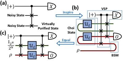
Figure 1: The logic for constructing VCP circuit, taking $M=2$ without loss of generality. (a) The circuit for VSP, consists of two copies of the noisy input state, a single control qubit initialised as $\ket{+}$, and a CSWAP gate. By measuring the control qubit in Pauli-$X$ basis, one can virtually prepare the purified state on the second register. (b) One possible circuit implementation of VCP, obtained from performing the VSP circuit in (a) on two copies of Choi states of the noisy channel. Each curved line at the input end stands for a $2N$-qubit maximally entangled state $\ket{\Phi^{+}}=\frac{1}{\sqrt{2^{N}}}\sum_{i=0}^{2^{N}-1}\ket{ii}$, which is used to prepare the Choi state of the noisy channel $\mathcal{U}_{\mathcal{E}}$. Then, the VSP circuit acts on two noisy Choi states to virtually obtain a purified Choi state. The curved line at the output end stands for Bell state measurement (BSM) post-selected on the all-zero result, which is for implementing the purified channel using the purified Choi state. (c) A circuit implementation of VCP, obtained from straightening the curved lines in green and red in (b). By measuring the control qubit in Pauli-$X$ basis, one can virtually implement the purified channel on the second register. This circuit is easily generalised to a larger value of $M$ by employing $M-1$ copies of maximally mixed state and changing SWAP to the $M$th order permutation as shown in Fig. 9(a).

We consider the case where our ideal operation is a unitary channel $\mathcal{U}$, but in practice we can only implement the noisy channel $\mathcal{U}_{\mathcal{E}}=\mathcal{E}\mathcal{U}$, which is the ideal operation $\mathcal{U}$ followed by the noise channel

$$\mathcal{E}=p_{0}\mathcal{I}+\sum_{i=1}^{4^{N}-1}p_{i}\mathcal{E}_{i}.$$ (1)

Here $N$ is the number of qubits, $\mathcal{I}$ stands for the identity channel, and $\mathcal{E}_{i}(\rho)=E_{i}\rho E_{i}^{\dagger}$ are the noise components. In line with the assumptions made in VSP [9, 8], we will assume $\mathcal{E}$ is Pauli noise with $E_{i}$ being Pauli operators and also $p_{0}>p_{i}$ for all $i$ (i.e. identity is the leading component). More general noise can be transformed into Pauli noise via Pauli twirling [18, 17] and the applicability of our method beyond Pauli noise is also discussed in Sec. E.2. Our target for VCP is consuming $M$ copies of $\mathcal{U}_{\mathcal{E}}$ to implement $\mathcal{U}_{\mathcal{E}^{(M)}}=\mathcal{E}^{(M)}\mathcal{U}$ with the purified noise channel $\mathcal{E}^{(M)}$ being

$$\mathcal{E}^{(M)}=\frac{1}{\sum_{i=0}^{4^{N}-1}p_{i}^{M}}\left(p_{0}^{M}\mathcal{I}+\sum_{i=1}^{4^{N}-1}p_{i}^{M}\mathcal{E}_{i}\right).$$ (2)

As $p_{0}$ is the leading term, the noise rate of $\mathcal{E}^{(M)}$ decays exponentially with $M$ as expected.

Based on the Choi–Jamiołkowski isomorphism, the Pauli noise channel $\mathcal{E}$ have a one-to-one correspondence to the Choi state $\rho_{\mathcal{E}}$ whose dominant eigenvector corresponds to the identity channel. It is easy to show that under Pauli noise, the Choi state of $\mathcal{E}^{(M)}$ is proportional to the $M$th power of the Choi state of $\mathcal{E}$: $\rho_{\mathcal{E}^{(M)}}=\nicefrac{{\rho_{\mathcal{E}}^{M}}}{{\Tr[\rho_{\mathcal{E}}^{M}]}}$, which can be obtained by performing state purification on $M$ copies of $\rho_{\mathcal{E}}$ [8, 9]. Similar arguments also apply to the Choi states of $\mathcal{U}_{\mathcal{E}^{(M)}}$ and $\mathcal{U}_{\mathcal{E}}$. Hence, the most straightforward way to implement $\mathcal{U}_{\mathcal{E}^{(M)}}$ is first using $M$ copies of $\mathcal{U}_{\mathcal{E}}$ to prepare $M$ copies of their Choi state; next purifying the Choi state of $\mathcal{U}_{\mathcal{E}^{(M)}}$ from them; and finally using this purified Choi state to implement the purified channel $\mathcal{U}_{\mathcal{E}^{(M)}}$.

The circuit of state purification is shown in Fig. 1(a), for which the control-qubit measurement outcome probability and the corresponding output state of the second register can be denoted as $p_{\pm}$ and $\rho_{\pm}$, respectively. As shown in Ref. [9, 8], the purified state is given as $p_{+}\rho_{+}-p_{-}\rho_{-}$, which can be virtually prepared for information extraction by simultaneously measuring the controlled qubit and the second register plus post-processing. As shown in Fig. 1(b), using the exact same circuit with the input noisy states being the Choi states of $\mathcal{U}_{\mathcal{E}}$, prepared by acting $\mathcal{U}_{\mathcal{E}}$ on one side of the maximally entangled states $\ket{\Phi^{+}}$, we can virtually obtain the Choi state of the purified channel $\mathcal{U}_{\mathcal{E}^{(M)}}$. This Choi state can be used to apply the purified channel $\mathcal{U}_{\mathcal{E}^{(M)}}$ on some input state $\rho$ using the technique of quantum teleportation. Specifically, we need to perform Bell state measurements (BSM) on input state $\rho$ and one side of the purified Choi state, post-select based on the measurement result, and measure the other side to extract the value of $\Tr[O\mathcal{U}_{\mathcal{E}^{(M)}}(\rho)]$.

Though conceptually simple, this method requires significant quantum and classical resources. It needs more than two times qubit overhead compared to VSP for preparing the Choi states. Furthermore, to transform a state into a channel through teleportation, one would require the $2N$-qubit Bell state measurement result to be all $0$, whose success probability decays exponentially with the number of qubits. As we have drawn the whole procedure using the circuit in Fig. 1(b) with tensor network notations, we notice that the circuit has some internal structures that allow us to further simplify it.

This circuit utilises $\ket{\Phi^{+}}$ multiple times including the preparation of Choi states and the BSM. In tensor network notation [24], $\ket{\Phi^{+}}$ and the BSM projector are represented by bending a straight line as shown in Fig. 1(b). In this way, by simply straightening the wires using tensor network rules, we can obtain a simplified circuit shown in Fig. 1(c), in which the first CSWAP gate goes before the action of two channels and the green open wire on the input is mapped to the maximally mixed state based on tensor network rules. This is a much more efficient circuit with the same qubit overhead as VSP with no post-selection needed. We have further proved algebraically that the circuit in Fig. 1(c) can achieve VCP and generalise it to $M$th order purification in Sec. A.1, giving rise to the first key results in VCP.

Theorem 1

Using a single input state $\rho$, a single control qubit initialised as $\ket{+}$, $M-1$ copies of maximally mixed state $\nicefrac{{\mathbb{I}_{2^{N}}}}{{2^{N}}}$, $M$ copies of the noisy channel $\mathcal{U}_{\mathcal{E}}=\mathcal{E}\mathcal{U}$, and two controlled permutation operations, the measurement result of Fig. 9(a) ($M$th order generalisation of Fig. 1(c)) gives

$$\frac{\langle X\otimes O\rangle}{\langle X\otimes\mathbb{I}_{2^{N}}\rangle}=\Tr\left[O\mathcal{E}^{(M)}\mathcal{U}(\rho)\right],$$ (3)

where $\mathcal{E}$ and $\mathcal{E}^{(M)}$ follow the relation of Eq. 1 and Eq. 2.

In the context of quantum error correction (QEC), the main part of the circuit in Fig. 1(c) shares a similar structure with flag fault-tolerance [19, 25], which detects circuit faults between the two probe operations from the control qubit. It can also be viewed as space-time checks (or detector) [26, 27] on the noisy channels using permutation symmetry. This is not surprising since the original VSP is partly inspired by the circuit for performing permutation symmetry checks on states [28, 29]. Such a pair of CSWAPs is also used in the circuit for quantum switches [30], error filtration [31], and superposed quantum error mitigation [32]. We will further discuss these connections in Sec. IV.

III Performance

III.1 Stronger error suppression in VCP

Just like VSP, the VCP protocol can suppress noise exponentially with more copies of the noisy channel, but there are also additional advantages arising from directly mitigating errors in quantum channels instead of states as outlined below.

III.1.1 Exponentially stronger error suppression for global noise

VCP offers stronger error suppression compared with VSP due to a lower error rate for each individual error component. Consider a $N$-qubit depolarising channel that has $P$ probability of mapping any input state into the maximally mixed state,

$$\mathcal{E}(\rho)=(1-P)\rho+P\frac{\mathbb{I}_{2^{N}}}{2^{N}}.$$ (4)

It contains approximately $4^{N}$ Pauli error components each with an error probability $4^{-N}P$. If the input state is a pure state, the output noisy state has approximately $2^{N}$ error components each with an error probability $2^{-N}P$. Therefore, if we perform $M$th order VCP and VSP on the channel and the output state, respectively, which use the same number of qubits and channels, the resultant error rate is suppressed by a factor of $(4^{N}/P)^{M-1}$ for the VCP and $(2^{N}/P)^{M-1}$ for the VSP. Therefore, VCP can suppress $2^{N(M-1)}$ times more errors than VSP, which is exponentially larger with the number of qubits and the order of purification.

Although we use a specific noise example here, the advantage of VCP over VSP applies to more general cases. Due to the larger dimensionality of channels compared to the corresponding states, different error components in a noise channel can be mapped into the same error component in a noisy state. Thus in general, the error probability of the leading error component in a noise channel is smaller than that of the resultant noisy state, leading to stronger error suppression when we purify the channel compared to the state. For practical quantum circuits, as we increase the depth of the circuit, the local noise will be scrambled into a form closer and closer to the global depolarising channel [14, 33], taking us closer to the improvement factor mentioned above.

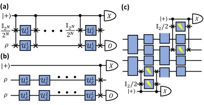
Figure 2: Comparison between VSP and VCP with $M=2$. (a) For a quantum circuit with depth $D$, VCP protocol can be applied layer-by-layer. Note that we use a single control qubit for all VCP layers here, but we can also use separate control qubits for them. (b) VSP protocol can only be performed once at the end of the quantum circuit with one control qubit and two identical copies. (c) VCP can target specific noisy gates in the quantum circuit.

III.1.2 Flexibility for applying to subsections of circuits.

With the ability to reset the maximally mixed state, VCP can be performed layer-by-layer, as shown in Fig. 2(a). On the other hand, VSP is only conducted at the end of the whole circuit as shown in Fig. 2(b), there are no existing protocols for performing VSP layer-by-layer. Such flexibility further enhances the scalability of VCP compared with VSP. For both VSP and VCP protocols to work, we need the target pure state (unitary) to be the dominant component of the noisy state (channel). Hence, for a given gate error rate, there is a maximum circuit depth beyond which VSP is not applicable as the noisy components start to dominate over the noiseless part. On the other hand, the advantages of VCP over the unmitigated circuit can be extended to any depths by simply adding more VCP layers. This is because while the full circuit error rate is high, VCP only cares about the error rate of individual layers that VCP acts on, which can be much smaller and is unchanged if we maintain the same layer depth as the circuit depth increases. As shown in the numerical experiment in Fig. 3(b), the fidelity of VSP drops to nearly zero when the circuit depth approaches the transition point. On the other hand, employing VCP layer by layer is able to maintain the fidelity at close to one over the whole range of circuit depth.

Even in the region where VSP is applicable and its dominant error component has the same error rate as that of VCP, there is still an advantage in applying layer-by-layer VCP. For simplicity, let us consider the example in which both the error channel and the corresponding noisy state have only one error component with the same error rate $P$ (more general cases are considered in Appendix C). This error component can be suppressed to $P^{M}$ using VSP. When applying VCP to the same circuit with the circuit divided into $L$ layers, the error rate of the dominant noise component in each layer is then $\sim P/L$, which can suppressed to $(P/L)^{M}$ after applying VCP to each layer. Thus the total error rate of the $L$-layer circuit after VCP is $L(P/L)^{M}$. This is $L^{M-1}$ smaller than VSP, which is exponential in $M$.

Furthermore, within each circuit layer, we can apply VCP to only a subset of qubits to purify the noisiest gate, as demonstrated in Fig. 2(c), while VSP can only mitigate incoherent noise for the entire state as a whole [9, 8, 34]. This offers great flexibility on the amount and the type of noise that we can mitigate, which can be particularly useful when the noise is concentrated only on a small number of qubits or some local gates. In such cases, applying VCP may require fewer CSWAPs and ancillary qubits compared to VSP while offering greater error suppression power.

It is worth mentioning that, if the noise channel of the circuit layer is a tensor product of local noisy channels, then applying VCP to the individual local channels will have the same effect as applying VCP to the entire circuit layers,

$$\left(\mathcal{E}_{1}\otimes\mathcal{E}_{2}\right)^{(M)}=\mathcal{E}_{1}^{(M)}\otimes\mathcal{E}_{2}^{(M)}.$$ (5)

Thus, it is possible to use one single control qubit to purify many independent quantum channels. As shown in Fig. 2(a), to purify a sequence of individual noisy gates, we can also use a single control qubit to remove the requirement for mid-circuit measurements for the VCP circuit, which can be important for many near-term quantum devices.

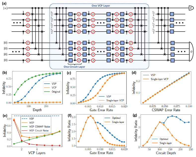
Figure 3: (a) The circuit for our numerical simulation with VCP applied. The main circuit is a four-qubit system initialised in the all-$0$ state evolving through a random circuit consisting of alternating layers of random single-qubit gates (blue boxes) and CNOT gates (two dots connected by a vertical line). The CNOT gates are affected by two single-qubit depolarising channels each with an error rate $p$ (red circles). The whole circuit is divided into $L$ VCP layers to perform the circuit shown in Fig. 2(a). In all numerical tests besides (b), every CSWAP gate is followed by three single-qubit depolarising channels each with an error rate $5p$. (b) The infidelities after VSP and VCP for different circuit depths without any CSWAP noise. The gate error rate is $p=0.005$ and the depth of each VCP layer is $20$. (c) The infidelities after VSP and single-layer VCP at different values of $p$. The circuit depth is set to be $80$. (d) The error rates caused by the CSWAP noise in VSP and single-layer VCP using the same circuit as (c), where we have removed the CNOT noise while keeping only the CSWAP noise. (e) The infidelity behaviour after VCP with different numbers of VCP layers for a circuit with a depth $240$ and a gate error rate $p=0.005$. The green and red lines represent cases without CNOT and CSWAP errors, respectively. (f) The infidelity ratios between VSP and single-layer VCP, and between VSP and VCP with the optimal number of VCP layers, at different gate noise rates with a circuit depth of $80$. (g) The infidelity ratios at different circuit depths with a fixed gate error rate of $p=0.005$.

III.2 Practical Implementation

So far we have not considered the noise in the CSWAPs needed for implementing VCP. Compared to VSP, single-layer VCP requires an additional layer of CSWAPs before the main circuit. Any noise happening after these additional CSWAPs can be absorbed into the main circuit noise and thus can be mitigated by VCP, especially when the noise is uncorrelated among the different qubits that the individual CSWAP acts on. In such cases, implementing single-layer VCP does not introduce much additional noise than VSP, but it is able to offer much stronger noise suppression as mentioned in Sec. III.1, making it almost always a preferred choice in practical implementations. We perform numerical experiments with the CSWAP error rate set to five times the two-qubit gate error rate, since we need five two-qubit gates to construct a CSWAP gate [35]. In Fig. 3(c), we see that indeed single-layer VCP can offer much stronger error suppression than VSP in the presence of CSWAP noise for the full range of gate error rate. In Fig. 3(d), we further plot the corresponding circuit error rate due to CSWAP for both single-layer VCP and VSP, which are approximately the same as expected despite the additional layer of CSWAPs in single-layer VCP.

Moving onto multi-layer VCP discussed in the last section, the error rate after VCP without CSWAP noise, denoted as $P_{\mathrm{c,cir}}(L)$, will decrease with the number of VCP layers $L$ and thus we should have as many VCP layers as possible. However, the error rate due to CSWAPs, denoted as $P_{\mathrm{c,sw}}(L)$, increases with the number of VCP layers $L$. Therefore, instead of increasing the number of layers $L$ indefinitely, we will only increase $L$ until the approximate optimal point $L^{*}$ (see Appendix C for the exact optimal point) such that

$$P_{\mathrm{c,cir}}(L^{*})\sim P_{\mathrm{c,sw}}(L^{*}).$$ (6)

Increasing VCP layers beyond this point will increase the total errors since the CSWAP errors $P_{\mathrm{c,sw}}$ start to dominate. This is illustrated in Fig. 3(e) where we have plotted how $P_{\mathrm{c,cir}}$, $P_{\mathrm{c,sw}}$ and the total error rate $P_{c,\mathrm{tot}}$ change with the number of VCP layers in a numerical experiment. We can see that the optimal number of VCP layers that minimise $P_{c,\mathrm{tot}}$ indeed occur around $P_{\mathrm{c,cir}}\sim P_{\mathrm{c,sw}}$.

In order to obtain expressions of the optimal number of VCP layers, we can zoom into each individual VCP layer whose depth is denoted as $d$. We will focus on the noise regime $dNp\ll 1$ such that the unmitigated error rate per VCP layer is well approximated by $dNp$, which can be suppressed to $P_{\mathrm{c,cir}}(L)/L\propto(dNp)^{M}$ using VCP. There are two layers of CSWAPs in each VCP layer and thus the corresponding error rate is simply proportional to the error rate of individual gate layer $P_{\mathrm{c,sw}}(L)/L\propto Np$. As mentioned above, the optimal number of layers, or equivalently, the optimal depth of each VCP layer $d^{*}$, can be reached when Eq. 6 is satisfied, which implies $P_{\mathrm{c,cir}}(L^{*})/L^{*}\sim P_{\mathrm{c,sw}}(L=L^{*})/L^{*}$ and thus:

$$(d^{*}Np)^{M}\propto Np\quad\Rightarrow\quad d^{*}\propto(Np)^{\frac{1-M}{M}}.$$ (7)

The arguments above are mainly for demonstrating the scaling of $d^{*}$ w.r.t. $p$. There is further dependence on $N$, through the number of error components, that is not shown here as discussed in Appendix C. If we denote the depth of the circuit as $D$, the optimal number of VCP layers is given as

$$L^{*}=D/d^{*}\propto D(Np)^{\frac{M-1}{M}}$$ (8)

For a fixed gate layer error rate $Np$, we have a fixed $d^{*}$ and thus the number of optimal VCP layers $L^{*}$ is linearly related to $D$. We use numerical experiments shown in Fig. 10 to validate our conclusion.

The total error rate of the circuit with the optimal number of layers is thus given as:

$$P_{c,\mathrm{tot}}(L^{*})\sim 2P_{\mathrm{c,sw}}(L^{*})=2\frac{P_{\mathrm{c,sw}}(L^{*})}{L^{*}}L^{*}\propto D(Np)^{\frac{2M-1}{M}}.$$

This error rate at the optimal number of layers is by definition smaller than that of single-layer VCP, which is in turn smaller than that of VSP in most cases as discussed above.

Now given the ideas of how VCP performs with the optimal number of layers, we can try to compare it against VSP. We will focus on the parameter regime where VSP is applicable and use $P_{\mathrm{s,cir}}$ and $P_{\mathrm{s,tot}}$ to denote the error rate after VCP without and with CSWAP noise, respectively. The ratio between the error rate achieved by VSP over that of VCP with the optimal layer number as shown in Appendix D is given as:

$$R=\frac{P_{\mathrm{s,tot}}}{P_{\mathrm{c,tot}}}\approx\frac{1}{2}{L^{*}}^{M-1}\frac{P_{\mathrm{s,cir}}}{P_{\mathrm{c,cir}}(L=1)}.$$ (9)

where $P_{\mathrm{s,cir}}/P_{\mathrm{c,cir}}(L=1)$ is simply the ratio between the error rate after VSP and single-layer VCP without any CSWAP noise. When looking at the individual factors in $R$, we see that $P_{\mathrm{s,cir}}/P_{\mathrm{c,cir}}(L=1)$ can increase exponentially with the number of qubits for global noise as discussed in Sec. III.1; while $L^{*}$ will increase linearly with the depth of the circuit $D$ and also increase with the gate error rate $p$ following Eq. 8. Since there is implicit exponential dependence on $M$ in $P_{\mathrm{s,cir}}/P_{\mathrm{c,cir}}(L=1)$ (see Appendix C), we also see that $R$ will increase exponentially with $M$.

It is worth emphasising that all the expressions in this section are mainly for gaining intuitions on the scaling behaviours of the various quantities rather than being the exact expressions. More explicit formulas and the relevant assumptions made are outlined in Appendix C. There we will also show that in some rare parameter regime, $P_{\mathrm{c,cir}}$ can increase with the increase of $L$ such that single-layer VCP is the best-performing option.

We have conducted a series of numerical experiments to see the exact factor of improvement we can obtain using VCP over VSP. As shown in Fig. 3(e) and (f), the ratio between the resultant infidelities using VSP over VCP is larger than $1$ throughout different gate error rates and different circuit depths, with the possibility of achieving up to $4$ times more error suppression in some region. Note that this is under a CSWAP noise that is $5$ times stronger than the gate error rate, which is close to the achievable experimental value [36, 37] for most of the gate error rates we explore.

Even though we have only performed $4$-qubit numerical simulations in this section ($9$-qubit if we include the control qubit and the ancillary qubits), we are performing experiments on a large enough circuit size such that the circuit fault rate (i.e. the average number of faults per circuit run) is of $\lambda\sim\order{1}$ and beyond. The circuit fault rate is the key quantity that determines the performance of QEM techniques [1] and $\lambda\sim\order{1}$ is expected to be the parameter regime that we will implement QEM in practice. Hence, our numerical experiments still provide a good indication of the performance of VCP in practice despite its small system size due to the use of a realistic circuit fault rate.

If all CSWAPs follow a similar error model, we can actually efficiently characterise the noise in the CSWAPs and try to mitigate their noise using probabilistic error cancellation [5]. In this way, we can remove almost all CSWAP noises to obtain the full benefit of VCP. Of course, we can also mitigate the CSWAP noise using zero-noise extrapolation [5, 7] which is shown to be effective in VSP [9].

Another challenge in the physical implementation is the connectivity required for the CSWAPs. This was extensively discussed in VSP [9], and the methods there are also applicable to VCP. In particular, the hardware architecture proposed in Ref. [38], which is applicable to silicon spin, trapped ions and neural atoms platforms, equips with native transversal gates between different quantum registers. Hence, in this architecture, all the CSWAPs in VCP can be applied transversely without any connectivity constraints if we use the VCP circuit variants with multiple control qubits proposed in Sec. E.1.

III.3 Sampling Overhead

As discussed, VCP is performed by measuring the observables outlined in Theorem 1. Compared to the unmitigated circuit, additional circuit runs (samples) are needed in order to obtain the VCP result since we are trying to extract useful information out of the noisy data. The factor of increase in the number of samples needed compared to the unmitigated circuit is called the sampling overhead. The sampling overhead for VCP can be obtained through the same arguments as the sampling overhead of VSP [9, 8], where the range of the effective random variable we used for expectation value estimation is increased by $P_{M}^{-1}$, with $P_{M}=\sum_{k=0}^{4^{N}-1}p_{k}^{M}$ being normalising constant of the purified channel in Eq. 2. Hence, using the Hoeffding’s inequality, the sampling overhead is given as

$$C_{\mathrm{em}}\sim P_{M}^{-2}.$$

This is similar to the sample complexity scaling obtained for VSP. A more exact expression is derived in Sec. A.3.

Analysis of the scaling of $C_{\mathrm{em}}$ follows the same arguments in Ref. [39], which gives an lower bound of $C_{\mathrm{em}}\sim P_{M}^{-2}\geq\frac{e^{M\lambda}}{1+(e^{\lambda}-1)^{M}}$ with $\lambda$ being the average number of errors in each circuit run (circuit fault rate). This bound is the same as VSP [1]. When performing layer-by-layer VCP, the sampling overhead for the whole circuit is simply the product of the sampling overhead for individual layers.

IV Generalisation and Combination with Quantum Error Correction

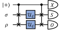
Figure 4: The VCP circuit with general ancillary input states and measurements.

IV.1 Connection to Existing Methods

For the VCP circuit in Fig. 1(c), there are other possible choices of ancillary input states beyond the maximally mixed state in order to achieve error mitigation. In fact, if the input state is a pure state $\rho=\outerproduct{\psi}{\psi}$, we can choose the ancillary input state to be the same as the main input state such that the first controlled-permutation operator acts trivially and can be removed. In this way, we have recovered the VSP circuit [9]. We have discussed in more detail how VSP fit into the general framework of VCP in Appendix F. In the context of state purification, noise can be further suppressed by measuring noisy projectors of the target state on the ancillary systems [40, 41, 42]. Adding ancillary measurements is a way to further generalise the VCP protocol.

We can consider a VCP circuit with a general ancillary input state $\sigma$ and measurement $S$ as shown in Fig. 4(a), which can also be extended to $M$ copies of the noisy channels. A particularly interesting choice of $\sigma$ and $S$ can be obtained via connections to quantum error correction.

IV.2 Merging with Quantum Error Corrections

In Sec. A.4, we have derived the expectation value of the circuit in Fig. 4. There we have shown that we can perform VCP as long as the input ancillary state $\sigma$ and ancillary measurement $S$ satisfy

$$\Tr(E_{i}U\sigma U^{\dagger}E^{\dagger}_{j}S)=\delta_{ij},$$ (10)

where $U$ is the target unitary. It is easy to verify that our earlier choice of $\sigma=\frac{\mathbb{I}_{2^{N}}}{2^{N}}$ and $S=\mathbb{I}_{2^{N}}$ indeed satisfy this condition for Pauli noise.

One particularly interesting choice of $\sigma$ and $S$ is found using the Knill-Laflamme condition for quantum error correction [23] for a Pauli channel $\mathcal{E}$ and a non-degenerate stabiliser code defined by the code space $\Pi_{C}$:

$$\Pi_{C}E^{\dagger}_{j}E_{i}\Pi_{C}=\delta_{ij}\Pi_{C}.$$ (11)

Note that being able to correct $\{E_{i}\}$ also implies that we can correct any linear combination of $\{E_{i}\}$. The identity $\mathbb{I}_{2^{N}}$ is always part of this correctable set, and we assume that $E_{0}=\mathbb{I}_{2^{N}}$ is the leading Kraus operator as discussed in Sec. II.

Let $\sigma_{C}$ be a state in the code space (i.e. $\sigma_{C}\Pi_{C}=\Pi_{C}\sigma_{C}=\sigma_{C}$), multiplying $\sigma_{C}$ on both side of Eq. 11 and taking the trace will give us:

$$\Tr(\sigma_{C}\Pi_{C}E^{\dagger}_{j}E_{i}\Pi_{C}) =\delta_{ij}\Tr(\sigma_{C}\Pi_{C})$$

$$\Tr(E_{i}\sigma_{C}E^{\dagger}_{j}) =\delta_{ij}$$ (12)

This is simply Eq. 10 with $U\sigma U^{\dagger}=\sigma_{C}$ and $S=\mathbb{I}_{2^{N}}$. In other words, if we want to mitigate the noise in some noisy operation $\mathcal{E}\mathcal{U}$, one valid choice of the ancillary state $\sigma$ is one that can be mapped by the ideal operation $\mathcal{U}$ into a code state $\sigma_{C}$ that can correct the noise $\mathcal{E}$. If instead of applying noisy operation, we want to send some state $\rho$ through a noisy channel $\mathcal{E}$. This means that we need to send a code state $\sigma_{C}$ that can correct $\mathcal{E}$ along with $\rho$ and perform the necessary VCP operations before and after the channel. In this way, we can suppress the noise in $\rho$ even though it is not in the code space. Furthermore, note that even though we are using the code state $\sigma_{C}$, we do not need to perform any stabiliser checks and corrections on it even after the noise is inflicted. No measurements need to be done on the ancillary code state $\sigma_{C}$.

If we allow for measurement on the ancillary code state, by measuring the code projector $\Pi_{C}$ on the ancillary code state at the end, we can actually remove all the noise in $\mathcal{E}$ instead of just purifying it. This is because

$$\Tr\left(E_{i}\sigma_{C}E_{j}^{\dagger}\Pi_{C}\right)=\Tr\left(\Pi_{C}E_{i}\Pi_{C}\sigma_{C}\Pi_{C}E_{j}^{\dagger}\Pi_{C}\right)=\delta_{i0}\delta_{j0},$$ (13)

which, as shown in Sec. A.4, can remove all the unwanted terms in the expectation value, leaving only the noiseless component. The measurement of the code projector $\Pi_{C}$ can be carried out through stabiliser measurement and post-selection. It can also be carried out at a lower hardware cost via single-qubit Pauli measurements and post-processing [43].

However, this additional post-selection of the ancilla stabiliser measurements will further increase the sampling cost of our protocol from $(\sum_{i}p_{i}^{2})^{-2}$ to $p_{0}^{-4}$ as shown in Sec. A.4, in line with the usual cost of quantum error mitigation [1] since we are now removing more errors. One may wonder if we can use the results of the stabiliser measurement at the end to improve the efficiency of the protocol. We have shown in Appendix B that we can indeed achieve this. After the stabiliser measurement, by applying the corresponding correction on the main register instead of on the ancillary register, we can effectively obtain the noiseless state in the main register with no additional post-selection. That is to say, using a QEC code as the ancillary register, measuring the stabiliser checks at the end and applying the corresponding correction on the main register, we can remove all the noise in the main register using the same sampling cost as 2nd order virtual purification.

IV.3 Connection to Flag Fault Tolerance

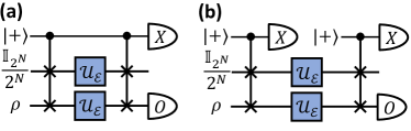
Figure 5: Circuits for measuring the SWAP-based detector. (a) Coherent SWAP detector. (b) Incoherent SWAP detector.

As mentioned before, the circuit structure we use for VCP is similar to the circuit used for flag fault-tolerance [19, 25] or spacetime checks in the recently proposed spacetime picture of viewing quantum error correction [27, 44, 26]. In VCP, we probe the noisy state before and after the noise channel using the CSWAPs operators and we measure the collective parity of these two checks using one control qubit as shown in Fig. 5(a) to see if the two probes are consistent with each other or not. A natural question to ask is whether we can perform the two checks one by one as shown in Fig. 5(b) and simply compare the check results in post-processing, which is how the conventional purely spatial codes operate. We will call the circuit in Fig. 5(a) and Fig. 5(b) as coherent and incoherent detectors, respectively.

As we have shown in Appendix G, both the coherent and incoherent detectors will remove the noise components in the detection region sandwiched between the CSWAPs. However, the incoherent detector will project the incoming state and the outgoing state into the eigensubspace of SWAP while the coherent detector will not act on the incoming states at all. As a result, VCP can only be performed using the coherent detector circuit.

It will also be very interesting to see how we can expand the application of such coherent detector circuits for symmetries beyond SWAP operations. For example, we can extend symmetry verification [10, 11] of problem-specific symmetries from the level of quantum states to channels. We can also try to find ways to apply this to the symmetry expansion and generalised subspace expansion protocols [45, 46] which are frameworks that further generalise the virtual purification scheme.

IV.4 Comparison to other techniques

We have discussed the main difference between VCP and other major QEM techniques in Sec. I and also made extensive comparisons between VCP and VSP in Sec. III. There are two other error suppression techniques in the name of error filtration (EF) [47, 31] and superposed quantum error mitigation (SQEM) [32] that also use multiple copies of the noisy channel. While in VCP we use one single control qubit to create interference between the original noise term and one other permuted noise term, EF and SQEM use a multi-qubit controlled register to create interference among multiple noise terms that correspond to all possible swappings between the main noise channel and the other noise channel copies. Then, they measure the control qubit and post-select the result, while in VCP, we keep all the results and perform post-processing. Due to these differences, EF and SQEM can only achieve suppression of noise linear in the number of copies of noisy channel $M$ instead of exponential in $M$ in VCP. Note that in SQEM [32] they also proposed incorporating active corrections to increase the efficiency of the protocol. However, they did not make the connection to QEC. Instead, they resorted to performing black-box optimisation for the selection of the input state, the measurement basis and the correction unitaries altogether. It is challenging to have a rigorous performance guarantee for such an optimisation routine and it can be very costly to implement as we increase the system size, and thus it is only suitable for small noisy gates.

Of course, rather than comparing VCP against these methods, it often makes more sense to combine the key ideas within them. We have mentioned in Sec. III about the effectiveness of using other QEM methods like probabilistic error cancellation and zero-noise extrapolation to remove the noise in the CSWAPs and the ancilla in VCP. We can also bring in ideas from EF to explore the possibility of using fewer registers for higher $M$ (at the cost of more control qubits). We can also try to apply the idea of using maximally mixed states and QEC code states as the ancillary input state from VCP to EF and SQEM, especially when applying to communication. It will also be interesting to look at VCP in other application scenarios like QRAM mentioned in Ref. [31].

V Application beyond computation

So far, we have been keeping all output states from the VCP circuit and post-processing them to virtually prepare the purified channel for recovering the measurement statistics. If we simply post-select the measurement outcome of the control qubit without further post-processing, we can physically obtain a quantum channel with higher purity from copies of noisy ones for tasks beyond expectation value estimation. As shown in Sec. A.2, by performing a post-selection on the control qubit, we have the following result.

Corollary 1

In the VCP circuit given in Fig. 9(a) without the measurement of the observable $O$. Suppose the $M-1$ ancillary registers are initialised in the maximally mixed state, and all of these $M$ registers are acted transversally by $M$ copies of the noisy channel $\mathcal{U}_{\mathcal{E}}$. After applying the quantum circuit, upon measuring $+$ on the control qubit, which occurs with probability $P_{+}=\frac{1}{2}\left(1+P_{M}\right)$, and with the ancillary system discarded, the effective channel acting on the main register is

$$\mathcal{U}_{\mathcal{E}_{+}}=\frac{1}{1+P_{M}}\left[\mathcal{U}_{\mathcal{E}}+P_{M}\mathcal{U}_{\mathcal{E}^{(M)}}\right],$$ (14)

where $P_{M}=\sum_{i=0}^{4^{N}-1}p_{i}^{M}$.

The protocol effectively mixes in some purified noise components $\mathcal{U}_{\mathcal{E}}^{(M)}$, improving the purity and the fidelity of the channel. One would notice that performing post-selection on the control qubit in this case shares a lot of similarities to performing quantum error detection using a space-time check as discussed in Appendix G.

The ability to physically purify a quantum channel can benefit applications where high-quality quantum resources are indeed necessary, such as high-fidelity entanglement distribution for quantum networks [48]. This is because the input state $\rho$ of the VCP circuit can be arbitrary states, including the subsystem of a large entangled state. In Fig. 6(a), we depict the simplest case with two users. Due to factors like platform hardware constraints and network topology, while some channel links are behaving normally, represented by the solid lines, some others may suffer from a high level of noise, represented by the dashed lines. Notably, not all the users in the network may suffer from a highly noisy channel link, such as $A_{2}$ in the figure. By applying the channel purification scheme in Corollary 1, the user $A_{1}$ can focus on the ill-behaved channel links and apply the channel purification scheme without disturbing the other user, resulting in a high-quality network for entanglement distribution. The channel purification scheme uses a single clean channel link to transmit one clean qubit for purifying arbitrarily large quantum channels. In practical situations, the clean qubit can be reasonably facilitated, such as by employing the path freedom in a linear optics system [49].

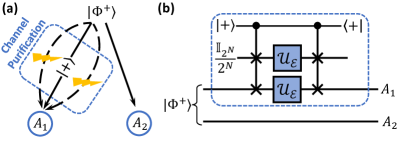
Figure 6: (a) Application of channel purification in entanglement distribution. Blue circles represent two users and $\ket{\Phi^{+}}$ is the entangled state that is distributed. In the case where only some of the quantum channels are noisy, denoted by the dashed lines with flashes, the relevant users can apply channel purification using one clean channel to obtain a purified channel. (b) The circuit for channel purification. Compared to the VCP circuit, we post-select on the measurement results of the control qubit and keep only the $\ket{+}$ outcome. The dashed blue box corresponds to the purification process in (a). From the perspective of entanglement-assisted quantum communication, $A_{2}$ corresponds to the reference system.

For high-fidelity entanglement distribution, our channel purification scheme can be advantageous compared to applying entanglement distillation after receiving multiple copies of a state. As stated above, the channel purification scheme is simply constrained to the users suffering from noisy links. On the other hand, typical entanglement distillation schemes [16], including those not restricted to local operations and classical communication [50], involve all the users over various nodes, who must collect copies of the distributed state and perform operations jointly. Moreover, in many applications, the channel links may be easily re-used, like the optical fibres in a communication network. On the contrary, preparing a highly entangled state can be costly. By purifying the channel links in advance, a high-quality entangled state can be shared among the users in every round of entanglement distribution. These features render our protocol to be resource-efficient. Moreover, the channel purification protocol permits us to activate some valuable quantum resources, such as entanglement, which is forbidden for typical entanglement distillation schemes.

We take a channel-theoretic viewpoint and quantitatively compare the channel behaviour before and after channel purification. The entanglement distribution scenario can be regarded as an entanglement-assisted quantum communication protocol [51, 52], as shown in Fig. 6(b). The entanglement source, which we call the sender in this protocol, sends a part of a maximally entangled state into the circuit, depicted as one half of $\ket{\Phi^{+}}$, and leaves the other part untouched, which we call the reference system. The two users $A_{1}$ and $A_{2}$, which we jointly call the receiver, collect the joint state of the main system and the reference system. The final joint state is the Choi state of the channel in the dashed blue box. For simplicity, we consider $\mathcal{U}_{\mathcal{E}}$ to be the depolarising channel characterized by Eq. 4, which may turn the state into the fully mixed state with probability $P$, and take $M=2$ copies of the noisy channel in the channel purification scheme. We consider a single-qubit channel ($N=1$) and a two-qubit channel ($N=2$), respectively.

We first quantify the state fidelity with respect to the maximal entangled state, $\bra{\Phi^{+}}\rho\ket{\Phi^{+}}$, with $\ket{\Phi^{+}}=\sum_{i=0}^{2^{N}-1}\ket{ii}/\sqrt{2^{N}}$ and $\rho$ being the distributed state. In Fig. 7(a), we depict the final state fidelity with respect to $P$ when it is directly transmitted through the noisy channel and transmitted through the purified channel. As can be seen from the curves in blue, after applying the channel purification, the state fidelity is boosted. In particular, in some range of $P$ where a direct state transmission breaks entanglement, the output state through a purified channel can become entangled. That is, the fidelity becomes higher than $0.5$ for $N=1$ and $0.25$ for $N=2$.

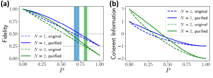
Figure 7: Channel performance before (dashed lines) and after (solid lines) channel purification. (a) The fidelity of the distributed state with respect to the maximally entangled state for different qubit numbers. Phenomena of entanglement activation are observed in ranges denoted by blue and green shadows. (b) The channel coherent information with respect to the maximally entangled state for different numbers of qubits.

From another perspective, the fact that the Choi state of the channel becomes entangled implies a nontrivial quantum channel capacity, where the Choi states of all entanglement-breaking channels are separated states [53]. As a figure of merit, we calculate the coherent information of the channels with respect to the maximally entangled state. For a channel $\mathcal{U}_{\mathcal{E}}$, the measure $I_{C}(\mathcal{U}_{\mathcal{E}},\ket{\Phi^{+}})$ is defined as

$$I_{C}(\mathcal{U}_{\mathcal{E}},\ket{\Phi^{+}})=S_{E}(\tr_{R}(\mathcal{U}_{\mathcal{E}}\otimes\mathcal{I}[\Phi^{+}]))-S_{E}(\mathcal{U}_{\mathcal{E}}\otimes\mathcal{I}[\Phi^{+}]),$$ (15)

where $\mathcal{U}_{\mathcal{E}}$ and the identity channel $\mathcal{I}$ each acts on a half of the state, $\Phi^{+}$ represents the density matrix of $\ket{\Phi^{+}}$, $S_{E}(\cdot)$ represents the von Neumann entropy, and the subscript $R$ represents the reference system. This measure can be viewed as a capacity measure for entanglement transmission and serves as a lower bound on the quantum channel capacity [54, 55, 56]. As seen from Fig. 7(b), the coherent information of the purified channel is also boosted after the purification scheme.

There are other schemes like error filtration [47, 57, 31] and coherent routing [58, 59, 60] that also use a control system to superpose channels coherently to combat the noise. However, the original error filtration scheme mainly works for communication tasks where the target channel is restricted to the identity channel. The coherent routing schemes require the knowledge of how the channel couples the transmitted state and the environment to maximize its efficacy. In contrast, our channel purification scheme works for a general target unitary. Besides, by employing a fully mixed state in the ancillary system, we can simply focus on the subsystem of interest, removing the additional requirement for a benchmark or even tomography of the channel.

VI Conclusion

In this article, we have introduced virtual channel purification (VCP), which is a way to virtually implement a purified channel using multiple copies of the noisy channels, and the infidelity of the purified channel is suppressed exponentially with more copies of the noisy channels. Compared to its state counterpart, virtual state purification (VSP), VCP can suppress global noise exponentially stronger in the number of qubits due to the larger dimensionality of channels compared to states. While VSP requires the ideal output state to be a pure state, VCP places no such restrictions as it directly purifies the noisy channel and thus can be applied to any input state. Furthermore, while VSP can only be applied to the entire quantum circuit as a whole, VCP can be applied in a layer-by-layer manner or even target specific gates in the circuits. This provides flexibility and, more importantly, removes the restriction in VSP that the noiseless component must be the dominant component for the noisy circuit output. In this way, VCP is applicable to much deeper and noisier circuits than VSP.

When considering the practical implementation of VCP, the single-layer variant only requires one additional layer of CSWAPs compared to VSP. Furthermore, the noise of this additional layer of CSWAP is naturally mitigated by VCP itself. We have seen in numerics that the errors due to CSWAPs are essentially the same for both VCP and VSP. Hence, single-layer VCP is almost always preferred over VSP due to its stronger noise suppression power at a similar implementation error cost. We can further optimise the number of VCP layers to outperform the single-layer variant. In numerical simulation across a range of circuit depths and gate error rates (with the CSWAP error rate five times stronger), optimal-layer VCP always outperform VSP and can offer up to 4 times more error suppression. The advantage is expected to be even stronger using more copies of noise channels and more qubits.

Thus far in the standard configuration of VCP, the additional copies of the noisy channels are acting on a maximally mixed input state at the ancillary registers. Using the Knill-Laflamme condition, we show that we can also perform purification using a quantum error correction (QEC) code state as the ancillary input state. Furthermore, if we are able to perform stabiliser checks on the ancillary register at the end of the circuit and post-select, we can remove all noise from the main register using just two copies of the noise channel. This comes with a higher sampling cost following the usual bias-variance trade-off in QEM. Now instead of post-selecting on the stabiliser check results of the ancillary register, if we perform correction on the main register based on these check results, we can actually remove all noise from the main register while paying only the sampling cost of the second-order VCP. This provides one of the first frameworks that seamlessly combines QEM and QEC beyond the concatenation of QEC and QEM [22, 21, 20]. Note that throughout this whole process, we are able to remove noise from the main register even though the input state of the main register is some arbitrary state that is not encoded at all.

Using the same circuit as VCP, but performing post-selection on the controlled qubit measurement results instead of post-processing, we can physically (instead of virtually) obtain a purified channel, which can then be applied to many tasks in quantum networks. For example in entanglement distribution, compared to previous works based on entanglement purification, our channel purification protocol does not require multipartite joint operations and multiple identical copies of the distributed states for local quantum noises. Furthermore, with a single clean channel to transmit a single clean qubit, our protocol can purify noisy channels with arbitrarily large dimensions and enable the activation of valuable quantum resources. The fact that our protocol is applicable to arbitrary incoming states and arbitrary incoherent noise also opens up the door for many other possible applications in communication.

Due to the presence of the controlled permutation operator at the beginning of the circuit which is coherently connected to the controlled permutation operator at the end, VCP actually lies outside the QEM frameworks presented for the discussion of the fundamental limits of QEM [61, 62, 63]. Hence, hopefully VCP can inspire a new range of QEM protocols outside these frameworks, like the combination with symmetry verification as we have mentioned in Sec. IV.3. One can also develop more general frameworks of QEM that incorporate VCP, which may have more desirable properties compared to the previous QEM framework. One promising way to do this is by finding deeper connections to QEC. One can try to generalise our arguments beyond non-degenerate codes, Pauli noise, and second-order purification or study the practical implementation of our protocol. It will also be interesting to search for other QEM methods that can be naturally merged with QEC beyond concatenation, similar to what we have done. This can be the start of a more general error suppression framework that naturally incorporates both QEM and QEC.

Appendix A VCP Protocol and its Generalisation

A.1 Validation of VCP Circuit

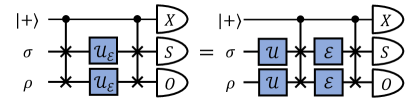
Figure 8: Under the assumption of $\mathcal{U}_{\mathcal{E}}=\mathcal{E}\mathcal{U}$, the unitary channel can be moved before the first CSWAP gate.

Here, we provide the proof for the validation of the VCP circuit, starting from the $M=2$ case. The channel of the noisy operation is $\mathcal{U}_{\mathcal{E}}=\mathcal{E}\mathcal{U}$. Since the tensor product of two identical unitaries $\mathcal{U}\otimes\mathcal{U}$ commutes with the controlled register-swap gate, we can perform our analysis of how the noise is mitigated by only analysing $\mathcal{E}$ (instead of $\mathcal{U}_{\mathcal{E}}$) while viewing the input states as $\mathcal{U}(\rho)$ and $\mathcal{U}(\sigma)$ as shown in Fig. 8.

Using a Kraus representation of the noise channel $\mathcal{E}(\rho)=\sum_{i=0}^{4^{N}-1}p_{i}E_{i}\rho E_{i}^{\dagger}$, the measurement result of Fig. 1(c) is

$$\expectationvalue{X\otimes O}$$ (16)

$$= \frac{1}{2}\sum_{i,j=0}^{4^{N}-1}\frac{p_{i}p_{j}}{2^{N}}\bigg{[}\bra{0}X\ket{0}\Tr\left(OE_{i}\rho E_{i}^{\dagger}\right)\Tr\left(E_{j}\mathbb{I}_{2^{N}}E_{j}^{\dagger}\right)$$

$$+\bra{1}X\ket{1}\Tr\left(OE_{j}\rho E_{j}^{\dagger}\right)\Tr\left(E_{i}\mathbb{I}_{2^{N}}E_{i}^{\dagger}\right)$$

$$+\bra{0}X\ket{1}\Tr\left(OE_{i}\rho E_{j}^{\dagger}\right)\Tr\left(E_{j}\mathbb{I}_{2^{N}}E_{i}^{\dagger}\right)$$

$$+\bra{1}X\ket{0}\Tr\left(OE_{j}\rho E_{i}^{\dagger}\right)\Tr\left(E_{i}\mathbb{I}_{2^{N}}E_{j}^{\dagger}\right)\bigg{]}.$$

As mentioned in the main text, we will focus on the case where $\mathcal{E}$ is a Pauli channel, thus $\frac{1}{2^{N}}\Tr\left(E_{i}E_{j}^{\dagger}\right)=\delta_{ij}$. Further using $\bra{0}X\ket{0}=\bra{1}X\ket{1}=0$ and $\bra{0}X\ket{1}=\bra{1}X\ket{0}=1$, the expectation value above becomes

$$\expectationvalue{X\otimes O}=\sum_{i=0}^{4^{N}-1}p_{i}^{2}\Tr\left(OE_{i}\rho E_{i}^{\dagger}\right)=P_{2}\Tr\left[O\mathcal{E}^{(2)}(\rho)\right].$$ (17)

By setting $O=\mathbb{I}_{2^{N}}$, we have the expectation value of the control qubit measurement as

$$\expectationvalue{X\otimes\mathbb{I}_{2^{N}}}=\sum_{i=0}^{4^{N}-1}p_{i}^{2}=P_{2}.$$ (18)

Combining Eqs. 17 and 18, we finish the proof of Theorem 1 by

$$\frac{\expectationvalue{X\otimes O}}{\expectationvalue{X\otimes\mathbb{I}_{2^{N}}}}=\frac{\sum_{i=0}^{4^{N}-1}p_{i}^{2}\Tr\left(OE_{i}\rho E_{i}^{\dagger}\right)}{\sum_{i=0}^{4^{N}-1}p_{i}^{2}}=\Tr\left[O\mathcal{E}^{(2)}(\rho)\right].$$ (19)

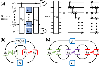
Figure 9: (a) The circuit for $M$th order VCP protocol, where $M-1$ copies of maximally mixed states and controlled $M$th order permutation gates, $D_{M}$, are employed. $D_{M}$ can be any highest-order permutation gate and thus can be constructed in many different ways. (b) and (c) The core tensor network diagram for the validation of the VCP circuit for $M=2$ and $3$. The solid black lines stand for matrix indices contraction and coloured tilde lines stand for summation over labelled indices.

As stated in the main context, by replacing the CSWAP gates with controlled $M$th order permutation gates and inputting $M-1$ copies of maximally mixed states, the VCP protocol can be generalised to a higher-order version. Following a similar derivation, one can show that the expectation value in Fig. 9(a) gives

$$\expectationvalue{X\otimes O}= \sum_{i_{1},\cdots,i_{M}=0}^{4^{N}-1}\frac{p_{i_{1}}\cdots p_{i_{M}}}{2^{N(M-1)}}\Tr\left(E_{i_{M}}\rho E_{i_{1}}^{\dagger}O\right)$$ (20)

$$\times\prod_{m=1}^{M-1}\Tr\left(E_{i_{m}}\mathbb{I}_{2^{N}}E_{i_{m+1}}^{\dagger}\right)$$

$$= \sum_{i=0}^{4^{N}-1}p_{i}^{M}\Tr\left(E_{i}\rho E_{i}^{\dagger}O\right).$$

Similarly, we have $\expectationvalue{X\otimes\mathbb{I}_{2^{N}}}=\sum_{i=0}^{4^{N}-1}p_{i}^{M}$ and $\nicefrac{{\expectationvalue{X\otimes O}}}{{\expectationvalue{X\otimes\mathbb{I}_{2^{N}}}}}=\Tr\left[O\mathcal{E}^{(M)}(\rho)\right]$.

Tensor network diagrams are introduced to illustrate the core ideas of our deviation, as shown in Fig. 9(b) and (c). To summarise, the controlled permutation gates together with the measurement of control qubit in Pauli-$X$ basis help to superpose multiple channels and extract terms where different Kraus operators of $\mathcal{E}$ act on different sides of $\rho$, such as $p_{i}p_{j}E_{i}\rho E_{j}^{\dagger}$. Then, the maximally mixed state helps to cancel the cross terms with $i\neq j$ and keep the diagonal terms with $i=j$, such that the weight of the target component can be amplified.

A.2 Post-selection

If we introduce post-selection to the VCP circuit, we can physically, instead of virtually, prepare a better quantum channel, as stated in Corollary 1. Similar to Eq. 16, if instead of measuring $X$ on the control qubit, we post-select only the $+$ result, while still measuring $O$ on the main register in Fig. 1, we then have

$$\expectationvalue{\outerproduct{+}{+}\otimes O}= \frac{1}{4}\sum_{i,j=0}^{4^{N}-1}\frac{p_{i}p_{j}}{2^{N}}\bigg{[}\Tr\left(OE_{i}\rho E_{i}^{\dagger}\right)\Tr\left(E_{j}\mathbb{I}_{2^{N}}E_{j}^{\dagger}\right)$$ (21)

$$+\Tr\left(OE_{i}\rho E_{j}^{\dagger}\right)\Tr\left(E_{j}\mathbb{I}_{2^{N}}E_{i}^{\dagger}\right)+c.c.\bigg{]}$$

which can be simplified to

$$\expectationvalue{\outerproduct{+}{+}\otimes O}= \frac{1}{2}\sum_{i=0}^{4^{N}-1}\left[p_{i}\Tr\left(OE_{i}\rho E_{i}^{\dagger}\right)+p_{i}^{2}\Tr\left(OE_{i}\rho E_{i}^{\dagger}\right)\right]$$ (22)

$$= \Tr\left[O\left(\frac{\mathcal{E}(\rho)+P_{2}\mathcal{E}^{(2)}(\rho)}{2}\right)\right].$$

And the probability of measuring $\ket{+}$ on the control qubit is

$$p_{+}= \expectationvalue{\outerproduct{+}{+}\otimes\mathbb{I}_{2^{N}}}=\frac{1}{2}(1+P_{2}).$$ (23)

We see that after post-selecting on the control qubit measurement, the main register has collapsed to a physical state

$$\rho_{+}=\frac{\mathcal{E}(\rho)+P_{2}\mathcal{E}^{(2)}(\rho)}{1+P_{2}}.$$ (24)

This result is easy to be generalized to VCP circuit with higher order $M$, as shown in Fig. 9(a). Thus, with post-selection and tracing out the ancillary systems, we can physically implement the following channel on the main register

$$\mathcal{E}^{(M)}_{+}=\frac{\mathcal{E}+P_{M}\mathcal{E}^{(M)}}{1+P_{M}}.$$ (25)

Noticing that $\mathcal{E}^{(M)}$ has the same Kraus components as $\mathcal{E}$ while with a higher weight of the target component. Thus, the noise rate of $\mathcal{E}^{+}$ is lower than $\mathcal{E}$, and we have physically acquired a better quantum channel.

A.3 Sample Complexity

Our estimator is constructed by division, $\nicefrac{{\expectationvalue{X\otimes O}}}{{\expectationvalue{X\otimes\mathbb{I}_{2^{N}}}}}=\Tr[O\mathcal{E}^{(M)}(\rho)]$. Notice that observables on the nominator and denominator commute with each other, so that we can measure both observables together in each circuit run. Suppose these two values are calculated using a number of $K$ circuit runs, then we can use the formula

$$\mathrm{Var}\left(\frac{x}{y}\right)\approx\frac{\mu_{x}^{2}}{\mu_{y}^{2}}\left(\frac{\mathrm{Var}(x)}{\mu_{x}^{2}}-2\frac{\mathrm{Cov(x,y)}}{\mu_{x}\mu_{y}}+\frac{\mathrm{Var}(y)}{\mu_{y}^{2}}\right)$$ (26)

to estimate the variance, where $x$ and $y$ stand for estimators of $\expectationvalue{X\otimes O}$ and $\expectationvalue{X\otimes\mathbb{I}_{2^{N}}}$, $\mu$ is the expectation value of the corresponding variable, and $\mathrm{Cov}$ stands for the covariance.

Starting with the simple case $M=2$, we can use the results in the last two sections to calculate $\mathrm{Var}\left(\frac{x}{y}\right)$. According to Eqs. 17 and 18, we have

$$\mu_{x}=P_{2}\Tr\left[O\mathcal{E}^{(2)}(\rho)\right]\ ,\ \mu_{y}=P_{2}.$$ (27)

According to the standard expressions for variance, we have

$$\mathrm{Var}(x)=\frac{1}{K}\left(\expectationvalue{\mathbb{I}_{2}\otimes O^{2}}-\expectationvalue{X\otimes O}^{2}\right)$$ (28)

Slightly changing the expression of Eq. 16, we have

$$\expectationvalue{\mathbb{I}_{2}\otimes O^{2}}$$ (29)

$$= \frac{1}{2}\sum_{i,j=0}^{4^{N}-1}\frac{p_{i}p_{j}}{2^{N}}[\bra{0}\mathbb{I}_{2}\ket{0}\Tr\left(O^{2}E_{i}\rho E_{i}^{\dagger}\right)\Tr\left(E_{j}\mathbb{I}_{2^{N}}E_{j}^{\dagger}\right)$$

$$+\bra{1}\mathbb{I}_{2}\ket{1}\Tr\left(O^{2}E_{j}\rho E_{j}^{\dagger}\right)\Tr\left(E_{i}\mathbb{I}_{2^{N}}E_{i}^{\dagger}\right)$$

$$+\bra{0}\mathbb{I}_{2}\ket{1}\Tr\left(O^{2}E_{i}\rho E_{j}^{\dagger}\right)\Tr\left(E_{j}\mathbb{I}_{2^{N}}E_{i}^{\dagger}\right)$$

$$+\bra{1}\mathbb{I}_{2}\ket{0}\Tr\left(O^{2}E_{j}\rho E_{i}^{\dagger}\right)\Tr\left(E_{i}\mathbb{I}_{2^{N}}E_{j}^{\dagger}\right)]$$

$$= \frac{1}{2}\sum_{i,j=0}^{4^{N}-1}\frac{p_{i}p_{j}}{2^{N}}[\Tr\left(O^{2}E_{i}\rho E_{i}^{\dagger}\right)\Tr\left(E_{j}\mathbb{I}_{2^{N}}E_{j}^{\dagger}\right)$$

$$+\Tr\left(O^{2}E_{j}\rho E_{j}^{\dagger}\right)\Tr\left(E_{i}\mathbb{I}_{2^{N}}E_{i}^{\dagger}\right)]$$

$$= \Tr\left[O^{2}\mathcal{E}(\rho)\right].$$

Substituting Eqs. 27 and 29 into Eq. 28, we have

$$\mathrm{Var}(x)=\frac{1}{K}\left\{\Tr\left[O^{2}\mathcal{E}(\rho)\right]-P_{2}^{2}\Tr\left[O\mathcal{E}^{(2)}(\rho)\right]^{2}\right\}$$ (30)

Similarly, we have

$$\mathrm{Var}(y)=\frac{1}{K}\left(\expectationvalue{\mathbb{I}_{2}\otimes\mathbb{I}_{2^{N}}}-\expectationvalue{X\otimes\mathbb{I}_{2^{N}}}^{2}\right)=\frac{1}{K}\left(1-P_{2}^{2}\right).$$ (31)

The calculation of covariance is similar to variance,

$$\mathrm{Cov}(x,y)=\frac{1}{K}\left(\expectationvalue{\mathbb{I}_{2}\otimes O}-\expectationvalue{X\otimes O}\expectationvalue{X\otimes\mathbb{I}_{2^{N}}}\right).$$ (32)

Changing the observable $O^{2}$ in Eq. 29 to $O$, we have

$$\mathrm{Cov}(x,y)=\frac{1}{K}\left\{\Tr\left[O\mathcal{E}(\rho)\right]-P_{2}^{2}\Tr\left[O\mathcal{E}^{(2)}(\rho)\right]\right\}.$$ (33)

Substituting Eqs. 27, 30, 31 and 33 into Eq. 26, we get the final expression of the variance

$$\mathrm{Var}\left(\frac{x}{y}\right)\approx \frac{1}{KP_{2}^{2}}\big{\{}\Tr\left[O^{2}\mathcal{E}^{(2)}(\rho)\right]$$ (34)

$$- 2\Tr\left[O\mathcal{E}^{(2)}(\rho)\right]\Tr\left[O\mathcal{E}(\rho)\right]+\Tr\left[O\mathcal{E}^{(2)}(\rho)\right]^{2}\big{\}}.$$

This result is easy to be generalised to any $M$ by changing $P_{2}$ and $\mathcal{E}^{(2)}$ to $P_{M}$ and $\mathcal{E}^{(M)}$, respectively. Considering that the observable has a bounded spectral norm, $\norm{O}_{\infty}\leq\mathrm{const}$, then the terms after $\frac{1}{KP_{M}^{2}}$ can also be bounded by some constant. Thus, to suppress the variance to $\epsilon^{2}$, the experiment times should scale as $K\sim\mathcal{O}\left(\frac{1}{\epsilon^{2}P_{M}^{2}}\right)$.

A.4 Circuit Generalisation

Till now, we only consider the case in which the ancillary register in Fig. 1(c) is initialised as the maximally mixed state and discarded at the end of the whole process. Now let us consider the circuit in Fig. 4, in which the ancillary system is initialised as some general state $\sigma$ and measured with the observable $S$ at the end of the circuit, the expectation value will be

$$\expectationvalue{X\otimes S\otimes O}$$ (35)

$$= \frac{1}{2}\sum_{i,j=0}^{4^{N}-1}p_{i}p_{j}[\bra{0}X\ket{0}\Tr\left(OE_{i}\rho E_{i}^{\dagger}\right)\Tr\left(SE_{j}\sigma E_{j}^{\dagger}\right)$$

$$+\bra{1}X\ket{1}\Tr\left(OE_{j}\rho E_{j}^{\dagger}\right)\Tr\left(SE_{i}\sigma E_{i}^{\dagger}\right)$$

$$+\bra{0}X\ket{1}\Tr\left(OE_{i}\rho E_{j}^{\dagger}\right)\Tr\left(SE_{j}\sigma E_{i}^{\dagger}\right)$$

$$+\bra{1}X\ket{0}\Tr\left(OE_{j}\rho E_{i}^{\dagger}\right)\Tr\left(SE_{i}\sigma E_{j}^{\dagger}\right)]$$

$$= \frac{1}{2}\sum_{i,j=0}^{4^{N}-1}p_{i}p_{j}\bigg{[}\Tr\left(OE_{i}\rho E_{j}^{\dagger}\right)\Tr\left(SE_{j}\sigma E_{i}^{\dagger}\right)+c.c.\bigg{]}.$$

Therefore, any choices of $\sigma$ and $S$ that satisfies

$$\Tr\left(SE_{i}\sigma E_{j}^{\dagger}\right)=\delta_{ij}$$ (36)

can be used to perform VCP. If one has enough knowledge of the noise, by suitably choosing the input state and/or the observable $S$, one can completely remove the noise. This is because if the state $\sigma$ and observable $S$ satisfy $\Tr(SE_{j}\sigma E_{i}^{\dagger})=\delta_{i0}\delta_{j0}$, the expectation value

$$\frac{\expectationvalue{X\otimes S\otimes O}}{\expectationvalue{X\otimes S\otimes\mathbb{I}_{2^{N}}}}=\frac{p_{0}^{2}\Tr\left(OE_{0}\rho E_{0}^{\dagger}\right)}{p_{0}^{2}}=\Tr\left(O\rho\right)$$ (37)

becomes the exact noiseless value.

Note that what we have discussed here can also be generalised to $M-1$ ancillary registers, each can come with a different input state $\sigma_{m}$ and measurement $S_{m}$ with the corresponding expectation value being:

$$\expectationvalue{X\otimes\bigotimes_{m=1}^{M-1}S_{m}\otimes O}=\sum_{i_{1},\cdots,i_{M}=0}^{4^{N}-1}\left(\prod_{m=1}^{M}p_{i_{m}}\right)$$ (38)

$$\quad\quad\quad\times\Tr\left(E_{i_{M}}\rho E_{i_{1}}^{\dagger}O\right)\prod_{m=1}^{M-1}\Tr\left(S_{m}E_{i_{m}}\sigma_{m}E_{i_{m+1}}^{\dagger}\right).$$

Appendix B Combining with Quantum Error Correction

Following the notations and arguments from Sec. A.4, but focusing on only the $M=2$ case, after measuring $X$ on the control qubit, we will virtually obtain the following state on the main and ancillary registers:

$$\sum_{i_{1},i_{2}}p_{i_{1}}p_{i_{2}}\underbrace{\left(E_{i_{2}}\rho E_{i_{1}}^{\dagger}\right)}_{\text{main}}\otimes\underbrace{\left(E_{i_{1}}\sigma_{C}E_{i_{2}}^{\dagger}\right)}_{\text{ancillary}}.$$ (39)

By performing stabiliser measurements on the ancillary register, we will project it into the $j$th syndrome subspace defined by $E_{j}\Pi_{C}E_{j}^{\dagger}$, and the resultant ancillary state will become

$$(E_{j}\Pi_{C}E_{j}^{\dagger})\left(E_{i_{1}}\sigma_{C}E_{i_{2}}^{\dagger}\right)(E_{j}\Pi_{C}E_{j}^{\dagger})$$

$$= E_{j}(\Pi_{C}E_{j}^{\dagger}E_{i_{1}}\Pi_{C})\sigma_{C}(\Pi_{C}E_{i_{2}}^{\dagger}E_{j}\Pi_{C})E_{j}^{\dagger}$$

$$= \delta_{i_{1},j}\delta_{i_{2},j}E_{j}\sigma_{C}E_{j}^{\dagger}.$$

Here we have made use of the Knill-Laflamme condition in Eq. 11. Substituting into Eq. 39, the resultant state after we perform stabiliser measurement on the ancillary state is

$$p_{j}^{2}\left(E_{j}\rho E_{j}^{\dagger}\right)\otimes\left(E_{j}\sigma_{C}E_{j}^{\dagger}\right).$$

Since we are considering a non-degenerate code that satisfies Eq. 11, the stabiliser measurement result will unambiguously tell us that the error inflicted is $E_{j}$. Hence, we can apply the corresponding correction $E_{j}$ to the main register and trace out the ancilla QEC state, giving us the state $p_{j}^{2}\rho$. The additional $p_{j}^{2}$ factor in front is due to the fact that we are measuring $X$ on the controlled qubit and thus the state is actually virtually obtained from post-processing. Averaging over all possible measurement outcome of the ancilla qubit, the effective output state is then

$$(\sum_{j}p_{j}^{2})\rho$$

The factor in front is the same as the normalising factor of 2nd-order purification. It is also the expectation value of the control qubit $X$ measurement, as discussed at the start of Sec. IV.2 where both registers are unmeasured. The inverse of this factor, $(\sum_{j}p_{j}^{2})^{-1}$, is then the increase of the range of the random variable we measure and thus $(\sum_{j}p_{j}^{2})^{-2}$ will be the sampling cost, which is the same as the usual 2nd-order purification.

Appendix C Optimal Number of Layers in VCP

C.1 Overall derivation

We will be considering a quantum circuit with $N$ qubits, depth $D$ and gate error rate $p$. The total number of gates in the whole circuit is approximately $ND$ with the circuit fault rate (average number of faults per circuit run) being $\lambda=NDp$. For the VCP considered in this section, the order of purification is denoted as $M$ and the number of VCP layers is denoted as $L$. For a large enough circuit, we can assume the errors in the circuit follow a Poisson distribution and thus the probability that the circuit is error-free is around $e^{-\lambda}$ [39]. Following similar arguments, for each VCP layer, the probability that the VCP layer is error-free is around $e^{-\lambda/L}$.

With noiseless CSWAPs, the error rate of the circuit after VCP is:

$$P_{\mathrm{c,cir}} \approx 1-\left[1-n_{c}^{1-M}\left(1-e^{-\lambda/L}\right)^{M}\right]^{L}$$ (40)

Here $n_{c}$ is the number of (dominating) error components in the channel. The discussion in Sec. III.1 focuses on the region where $\lambda\ll L$, in which $P_{\mathrm{c,cir}}\approx n_{c}L\left(\lambda/(n_{c}L)\right)^{M}$. For the expression in Eq. 40 to be accurate, we need the noiseless component to be dominating, which means $e^{-\lambda/L}\gg n_{c}^{-1}(1-e^{-\lambda/L})$ and thus $n_{c}+1\gg e^{\lambda/L}$. For global depolarising noise where $n_{c}=4^{N}$, we have $N\gg\lambda/(\ln(4)L)$ as a requirement. A similar but stronger restriction also applies to the corresponding expression for VSP in Eq. 49.

The number of CSWAPs in VCP is $2NML$ and each of them will have a gate error rate $\alpha p$, i.e. the CSWAP gate errors is $\alpha$ times stronger. As mentioned in Sec. III.2, the noise in half of these CSWAPs can be mitigated by VCP, thus the remaining average fault rate due to CSWAP after VCP is approximately $NML\alpha p=\alpha ML\lambda/D$. The corresponding error rate due to CSWAPs is then:

$$P_{\mathrm{c,sw}} \approx 1-e^{-\alpha ML\lambda/D}$$ (41)

At $L=1$ and small $M$, we usually expect $P_{\mathrm{c,cir}}(L=1)>P_{\mathrm{c,sw}}(L=1)$ since the main circuit is in general much deeper than the layers of additional CSWAPs in single-layer VCP ($D\gg M$). As we increase $L$, $P_{\mathrm{c,cir}}$ will decrease exponentially (we will discuss the case where $P_{\mathrm{c,cir}}$ is not always decreasing in Sec. C.4) while $P_{\mathrm{c,sw}}$ will increase (at first linearly). We will increase the number of layers until $P_{\mathrm{c,cir}}(L^{*})\sim P_{\mathrm{c,sw}}(L^{*})$ because beyond this point $P_{\mathrm{c,sw}}$ will dominate and the overall errors will increase with further increase in $L$. At this optimal $L^{*}$, the overall error rate after VCP

$$\begin{split}P_{\mathrm{c,tot}}(L)&=P_{\mathrm{c,cir}}(L)+P_{\mathrm{c,sw}}(L)\end{split}$$ (42)

will be minimised. The exact number of optimal layers should be obtained by taking the derivative of the total error rate and setting it to zero, which can be done numerically. In order to obtain an analytical expression, we will obtain an approximate optimal number of layers based on the arguments above by solving:

$$P_{\mathrm{c,sw}}(L^{*}) =P_{\mathrm{c,cir}}(L^{*})$$

$$e^{-\alpha ML^{*}\lambda/D} =\left[1-n_{c}^{1-M}\left(1-e^{-\lambda/L^{*}}\right)^{M}\right]^{L^{*}}$$

$$L^{*} =-\lambda/\ln(1-n_{c}^{\frac{M-1}{M}}\left(1-e^{-\alpha M\lambda/D}\right)^{\frac{1}{M}})$$ (43)

Following this assumption of $P_{\mathrm{c,sw}}(L^{*})=P_{\mathrm{c,cir}}(L^{*})$, the overall error after VCP at the optimal layer number is then given as:

$$\begin{split}P_{\mathrm{c,tot}}(L^{*})&=P_{\mathrm{c,cir}}(L^{*})+P_{\mathrm{c,sw}}(L^{*})\\ &=2P_{\mathrm{c,sw}}(L^{*})=2P_{\mathrm{c,cir}}(L^{*})\end{split}$$ (44)

which can be expressed into more explicit form by substituting Eq. 43 into Eqs. 40, 41 and 44.

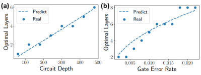
Figure 10: (a) shows the scaling of optimal layers with circuit depth, where we consider the same four-qubit random unitary circuit as in the main context with gate error rate $p=0.005$. (b) shows the scaling of optimal layers with gate error rate, with circuit depth $D=240$.

C.2 Small noise limit

An interesting limit to consider is when $n_{c}^{M-1}\alpha M\lambda/D\ll 1$ which is true for many practical cases. In this case, we have

$$L^{*}\approx\lambda\left(\frac{D}{\alpha Mn_{c}^{M-1}\lambda}\right)^{1/M}=D\left(\alpha M\right)^{-\frac{1}{M}}\left(\frac{Np}{n_{c}}\right)^{\frac{M-1}{M}}$$

For a fixed gate layer error rate $Np=\lambda/D$, we have $L^{*}$ grows linearly with $D$. On the other hand, at fixed $D$, we have $L^{*}\propto(Np)^{1/2}$ at $M=2$. We indeed see such trends in the numerical experiments in Fig. 10. The mismatch is mainly due to rounding $L^{*}$ to the nearest integer.

The optimal depth per VCP layer is given as:

$$d^{*}=D/L^{*}\approx(\alpha M)^{\frac{1}{M}}\left(\frac{n_{c}}{Np}\right)^{\frac{M-1}{M}}.$$ (45)

which is independent of $D$ and only determined by the error rate in each gate layer $Np$.

By noting that $P_{\mathrm{c,sw}}(L^{*})=P_{\mathrm{c,cir}}(L^{*})$ implies:

$$n_{c}^{1-M}\left(1-e^{-\lambda/L^{*}}\right)^{M}=1-e^{-\alpha M\lambda/D}$$

Further using the fact that $n_{c}^{M-1}\alpha M\lambda/D\ll 1$ implies $\alpha M\lambda/D\ll 1$, we can then obtain

$$n_{c}^{1-M}\left(1-e^{-\lambda/L^{*}}\right)^{M}=\alpha M\lambda/D\ll 1$$

This enable us to further simplify the expression of Eq. 40 and Eq. 41 at $L=L^{*}$ to

$$P_{\mathrm{c,cir}}(L^{*}) \approx L^{*}n_{c}^{1-M}\left(1-e^{-\lambda/L^{*}}\right)^{M}$$

$$P_{\mathrm{c,sw}}(L^{*}) \approx\alpha ML^{*}\lambda/D$$

Hence, the total error rate is

$$P_{\mathrm{c,tot}}(L^{*}) =P_{\mathrm{c,cir}}(L^{*})+P_{\mathrm{c,sw}}(L^{*})$$

$$\approx 2P_{\mathrm{c,cir}}(L^{*}) =2L^{*}n_{c}^{1-M}\left(1-e^{-\lambda/L^{*}}\right)^{M}$$ (46)

$$\approx 2P_{\mathrm{c,sw}}(L^{*}) =2\alpha ML^{*}\lambda/D$$ (47)

Using the expression of $L^{*}$, we can simplify this to

$$P_{\mathrm{c,tot}}(L^{*}) =2\alpha ML^{*}\lambda/D$$

$$=2D\left(\frac{\alpha M}{n_{c}}\right)^{\frac{M-1}{M}}\left(Np\right)^{\frac{2M-1}{M}}$$

C.3 Alternative Derivation

From Eq. 45, we see that the optimal depth of each VCP layer is solely determined by the error rate of each gate layer and is independent of the overall depth of the circuit. Deeper circuits simply mean more repetition of these VCP layers of optimal depth. Hence, unsurprisingly the optimal depth of the circuit can be derived by looking at only individual VCP layers without considering the whole circuit. Denoting the depth of the VCP layer as $d$, then the unmitigated error rate of each VCP layer is around $dNp$ in the small noise regime of $dNp<1$. In each VCP layer, there is $2MN$ CSWAPs with error rate $\alpha p$ and as mentioned before, only half of them will contribute to the CSWAP errors, thus the CSWAP error rate in each VCP layer is around $MN\alpha p$ in the small noise regime. In such a way, the total error rate per unit depth after applying VCP to the layer is

$$P_{c,\mathrm{tot}}/D=d^{-1}\left(n_{c}^{1-M}(dNp)^{M}+MN\alpha p\right)$$ (48)

Taking the derivative against $d$ and set it to $0$ we can obtain

$${d^{*}}^{-2}(MN\alpha p) =(M-1){d^{*}}^{M-2}n_{c}^{1-M}(Np)^{M}$$

$$d^{*} =\left(M-1\right)^{-\frac{1}{M}}(\alpha M)^{\frac{1}{M}}\left(\frac{n_{c}}{Np}\right)^{\frac{M-1}{M}}$$

We see that this is the same as Eq. 45 with an additional factor of $(M-1)^{-1/M}$ since we are taking the derivative rather than simply setting the two noise terms to be the same. Note that $(M-1)^{-1/M}=1$ for the most practical $M=2$ case.

C.4 Further considerations

Note that there are still some factors we have not taken into account in the above analysis. The number of channel noise components per VCP layer $n_{c}$ should be dependent on the depth per VCP layer $d$. Furthermore, we have not considered the simultaneous occurrence of errors in both the circuit and CSWAPs such that the total error rate for VCP is $P_{\mathrm{c,cir}}(L^{*})+P_{\mathrm{c,sw}}(L^{*})-P_{\mathrm{c,cir}}(L^{*})P_{\mathrm{c,sw}}(L^{*})$ and similarly for VSP. Moreover, the Poisson approximation we made for noise rate may not be fully suitable for some extreme cases. For the CSWAP noise, only the noise acting on the register that we are going to measure will have the strongest effect, at least for CSWAPs at the end of the circuit. For the parameter regime that we consider, these should not change any qualitative conclusion we draw in any significant way.

There is another assumption that we have not mentioned in the analysis above, that is, $P_{\mathrm{c,cir}}$ always decreases as $L$ increases. Or equivalently, with noiseless CSWAPs, the error rate per unit depth decreases as $d$ decreases. This is actually only true in specific parameter regimes. Let us look at the error rate per unit depth with noiseless CSWAPs without taking the small noise limit:

$$P_{\mathrm{c,cir}}/D \approx d^{-1}n_{c}^{1-M}\left(1-e^{-dNp}\right)^{M}$$

At small $d$, we have $P_{\mathrm{c,cir}}/D\approx\left(\frac{dNp}{n_{c}}\right)^{M-1}Np\propto d^{M-1}$, which increases as $d$ increase. This is the region that we have considered before. However, if we look at large $d$, we have $P_{\mathrm{c,cir}}/D\approx n_{c}^{1-M}d^{-1}$ which decreases as $d$ increase.

To find the transition point, we can differentiate $P_{\mathrm{c,cir}}/D$ against $d$:

$$\partialderivative{d}(P_{\mathrm{c,cir}}/D) \approx n_{c}^{1-M}d^{-2}\left(1-e^{-dNp}\right)^{M-1}$$

$$\quad\times\left((1+MdNp)e^{-dNp}-1\right)$$

This will be $0$ at a threshold value of $d_{th}Np<1.256$ for $M=2$. When $dNp<1.256$, we have $1+MdNp>e^{dNp}$ and thus $\partialderivative{d}(P_{\mathrm{c,cir}}/D)>0$ and $P_{\mathrm{c,cir}}/D$ increases as $d$ increases as expected. However, when $dNp>1.256$, we have $\partialderivative{d}(P_{\mathrm{c,cir}}/D)<0$ and $P_{\mathrm{c,cir}}/D$ decreases as $d$ increases.

Hence, when the circuit fault rate $\lambda=DNp<1.256$, then we naturally have $dNp<1.256$ and all of our arguments above are valid. On the other hand, if we have $\lambda=DNp>1.256$, then the optimal $d^{*}$ we found through setting the derivative of the total error to $0$ will always be on the side of $d^{*}Np<1.256$ (since only on this side we have a positive gradient cancel with a negative gradient of the CSWAP noise). On the side of $DNp<1.256$, the smallest error is always given by $d=D$ since the error decreases with the increase of $d$. Hence, all we need to do is to compare $d^{*}$ with $d=D$ to see which one is a better solution. As $M$ increases, the threshold value for $dNp$ will increase and thus the threshold value for $DNp$ will decrease.

Appendix D Comparison between VSP and VCP

D.1 Applicability of VSP and VCP

Here we follow the same notations outlined in Sec. C.1 to consider when is VSP and VCP applicable, respectively. We are applying VCP to individual VCP layers, thus we only need to look at the requirement on the individual layers. While we want to increase the layer number so that the dominant component per layer becomes the noiseless component, we also want to restrict the layer number so that the number of gates per layer is large compared to the number of CSWAPs per layer $2MN$, to minimise the damages due to CSWAP noise. We will use $n_{c}$ to denote the number of (leading) error components in the noise channel. In order for VCP to work, we need the identity component to be leading, i.e. $e^{-\lambda/L}>(1-e^{-\lambda/L})/n_{c}$, which means $\ln(n_{c}+1)>\lambda/L$. For global depolarising noise where $n_{c}+1=4^{N}$, we have $2N\ln(2)>\lambda/L$ as requirement. Using $\lambda=DNp$ we have

$$\frac{D}{L}=d<\frac{2\ln(2)}{p}$$

as the requirement, where $d=D/L$ is the depth per VCP layer. If $p=0.01$, then we can have $D/L$ up to $60$, which is much more than the depth of the CSWAPs $2M$ for $M=2$ and thus the number of gates per layer is much larger than the numbers of CSWAPs. The restriction on VSP is essentially the same with $L=1$ and $n_{c}=2^{N}$, i.e. we have

$$D_{\mathrm{vsp}}<\frac{\ln(2)}{p}$$

This places a hard bound on the depth of the circuit for a given gate error rate for VSP, while such depth bound only applies to the individual VCP layers in VCP and we can apply it to circuits of arbitrary depth by simply increasing the number of VCP layers.

D.2 Comparing Error Suppression of VSP and optimal VCP

Here we will consider the region where that noise is not so large such that VSP is still applicable, which also implies that VCP is also applicable. Following the same argument as Sec. C.1, the error rate of the circuit after $M$th order VSP without CSWAP noise and the error rate due to the CSWAPs are:

$$P_{\mathrm{s,cir}} \approx n_{s}^{1-M}\left(1-e^{-\lambda}\right)^{M}$$ (49)

$$P_{\mathrm{s,sw}} \approx 1-e^{-\alpha M\lambda/D}$$ (50)

respectively. Here $n_{s}$ is the number of (dominating) error components in the state. Note that $P_{\mathrm{s,cir/sw}}$ is the same as $P_{\mathrm{c,cir/sw}}$ with $L=1$ and $n_{c}=n_{s}$. In general we have $n_{c}\geq n_{s}$ as discussed in the main text, and thus $P_{\mathrm{c,cir}}<P_{\mathrm{s,cir}}$.

The ratio between the error rate after VSP and optimal-layer VCP is:

$$R =\frac{P_{\mathrm{s,cir}}+P_{\mathrm{s,sw}}}{P_{\mathrm{c,cir}}(L^{*})+P_{\mathrm{c,sw}}(L^{*})}\approx\frac{P_{\mathrm{s,cir}}}{2P_{\mathrm{c,cir}}(L^{*})}+\frac{P_{\mathrm{s,sw}}}{2P_{\mathrm{c,sw}}(L^{*})}$$

$$\geq\frac{P_{\mathrm{s,cir}}}{2P_{\mathrm{c,cir}}(L^{*})}$$ (51)

In another word, this is lower-bounded by the improvement of optimal-layer VCP over VSP with noiseless CSWAPs divided by $2$.

Starting from the small noise limit in Sec. C.2 where $\alpha M\lambda/D\ll 1$, this implies that $P_{\mathrm{s,sw}}\approx M\lambda/D\ll 1$. Hence, the resultant error ratio between VSP and VCP using Sec. D.2 is then

$$\frac{P_{\mathrm{s,cir}}}{2P_{\mathrm{c,cir}}(L^{*})}=\frac{1}{2L^{*}}\left(\frac{n_{c}}{n_{s}}\right)^{M-1}\left(\frac{1-e^{-\lambda}}{1-e^{-\lambda/L^{*}}}\right)^{M}$$

For small $\lambda$ such that $\lambda\ll L^{*}$ (i.e. $d^{*}Np\ll 1$), we have:

$$R\approx\frac{1}{2}{L^{*}}^{M-1}\left(\frac{n_{c}}{n_{s}}\right)^{M-1}$$

which is always larger than $1$ if $n_{c}\geq n_{s}$ and $L\geq 2$ (given that $M\geq 2$).

If we assume weak dependence of $n_{c}$ on $L$, then $(n_{c}/n_{s})^{M-1}$ is approximately the improvement of single-layer VCP over VSP with noiseless CSWAPs using Eqs. 40 and 49

$$\left(\frac{n_{c}}{n_{s}}\right)^{M-1}\approx\frac{P_{\mathrm{s,cir}}}{P_{\mathrm{c,cir}}(L=1)}.$$

Hence, the $R$ can be rewritten as:

$$R\approx\frac{1}{2}{L^{*}}^{M-1}\frac{P_{\mathrm{s,cir}}}{P_{\mathrm{c,cir}}(L=1)}.$$

Appendix E Practical Considerations

E.1 Circuit Variants with Separate Control Qubits

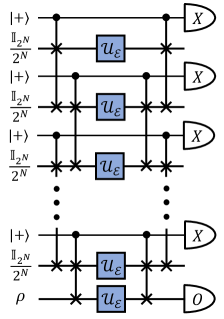
Figure 11: Circuit for virtual channel purification with separate control qubits for each CSWAP.

Instead of having one control qubit for all controlled register-swaps, we can also have a control qubit for each pair of controlled register-swaps acting between a given pair of registers. In Eq. 20 from Fig. 9(a), the right Kraus operator is a cyclic permutation of the left Kraus operator. The new output from Fig. 11 will be a superposition of different terms with the right Kraus operator being a different derangement of the left Kraus operator. The end result when we remove all the cross terms in virtual channel purification will be the same as Eq. 20. The benefit of using separable control qubits is that one can choose an optimal permutation operator $D_{M}$ in Fig. 9(a) to achieve a constant circuit depth.

The validation of Fig. 11 requires the fact that for a circuit that applies the whole set of linear nearest neighbour swaps in a random order, the whole circuit is always a derangement operation. This can be shown by realising that the qubit at position $i$ is touched by only two swaps in the entire circuit. One takes it to $i+1$ and the other takes it to $i-1$. If the first swap it meets takes it to $i+1$, then the only next possible swap that it can meet at $i+1$ is the one that goes from $i+1$ to $i+2$ since the other swap that goes from $i+1$ to $i$ is already used. Hence, in this way, the qubit can only remain at $i+1$ or increase its index to $i+2$. If the first swap it meets takes it to $i-1$, then it can only remain at $i-1$ or decrease its index to $i-2$. The qubit will never end up back in its original position $i$ and thus the circuit we show can “derange” the qubit indices.

For a given controlled register-swap, instead of just using one control qubit and performing CSWAP between all of the corresponding qubit pairs within different registers, we can assign one control qubit for each pair of the corresponding qubit and perform the CSWAP using that dedicated control qubit as shown in Fig. 12. The overall control qubit measurement outcome is simply the product of the measurement of all control qubits. This can be done because the swap operations between different qubit pairs commute with each other, and thus it does not matter whether we perform it on the left or right Kraus operators since they are all the same when we take the trace.

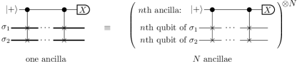
Figure 12: Circuit implementing controlled register-swaps using one control qubit can be replaced by a circuit using one control qubit for each pair of corresponding qubits. The overall control qubit measurement outcome is simply the product of the measurement of all control qubits.

E.2 Deviation from Pauli Noise Model

A given noise channel $\mathcal{E}$ acting on a $2^{N}$ dimensional Hilbert space can always be written in the normalised Kraus representation:

$$\mathcal{E}(\rho)=\sum_{i=0}^{4^{N}-1}p_{i}E_{i}\rho E_{i}^{\dagger}=\sum_{i=0}^{4^{N}-1}p_{i}\mathcal{E}_{i}(\rho)$$ (52)

with non-negative $p_{i}$ and normalised Kraus operators $\Tr(E_{i}^{\dagger}E_{i})=2^{N}$. The trace-preserving condition of the Kraus operators implies that $\sum_{i}p_{i}=1$. We have used the calligraphic font $\mathcal{E}_{i}$ to denote the channel corresponding to the operator $E_{i}$. Without loss of generality, we will assume all Kraus operators are ordered in descending order of $p_{i}$, i.e. $p_{0}\geq p_{1}\cdots p_{4^{N}-1}\geq 0$.

Just like regular Kraus representation, the normalised version in Eq. 52 is not unique for a given quantum channel. We will look at noise channels that, in at least one of their normalised Kraus representation, have their dominant Kraus operator $E_{0}$ being the identity operator $\mathbb{I}_{2^{N}}$, i.e. $p_{0}>p_{1}$ and $E_{0}=\mathbb{I}_{2^{N}}$:

$$\mathcal{E}=p_{0}\mathcal{I}+\sum_{i=1}^{4^{N}-1}p_{i}\mathcal{E}_{i}$$ (53)

We will call such a channel the identity-dominant channel, with the corresponding normalised Kraus representation being the identity-dominant Kraus representation. Note that the identity-dominant Kraus representation is not unique.

Identity-dominant channels become stochastic noise [64] when one of the identity-dominant Kraus representation coincide with the canonical Kraus representation of the channel, such that the Kraus operators in Eq. 1 are orthogonal to each other

$$\Tr(E_{i}E_{j}^{\dagger})=\delta_{ij}2^{N}.$$ (54)

Stochastic noise contains Pauli noise [65] (including dephasing and depolarising noise) that we have discussed and also more general mixed-unitary noise model that contains identity component.

Our purification scheme can be easily applied to stochastic noise channels beyond Pauli noise. For stochastic noise that satisfies Eq. 54, we can use the maximally mixed ancillary state $\sigma=\mathbb{I}_{2^{N}}/2^{N}$ to satisfy the purification condition in Eq. 10. However, in general the purified channel in the form of Eq. 2 is not properly normalised because in general $\sum_{i}p_{i}E_{i}^{\dagger}E_{i}=\mathbb{I}_{2^{N}}$ does not imply $P_{M}^{-1}\sum_{i}p_{i}^{M}E_{i}^{\dagger}E_{i}=\mathbb{I}_{2^{N}}$. In order to normalised it, we need to measure a normalising constant for a given input $\rho$ by simply setting $O=\mathbb{I}_{2^{N}}$. However, it is possible that even the unnormalised version will already give us a better output than the noisy version. This can be left for future investigation.

Similar to VCP, our method will also suffer from coherent mismatch when there is coherent noise in the target noise channel [8, 9]. Though such coherent noise is expected to be small for circuits of practical sizes [13].

E.3 Tensor Product of Channels

Given a product of two noise channels $\mathcal{E}$ and $\mathcal{F}$, their tensor product is simply

$$\mathcal{E}\otimes\mathcal{F} =\left(\sum_{i=0}^{4^{N}-1}p_{i}\mathcal{E}_{i}\right)\otimes\left(\sum_{j=0}^{4^{N}-1}q_{j}\mathcal{F}_{j}\right)$$

$$=\sum_{i,j=0}^{4^{N}-1}p_{i}q_{j}\mathcal{E}_{i}\otimes\mathcal{F}_{j}.$$

If we perform purification on $\mathcal{E}\otimes\mathcal{F}$, we have

$$\quad(\mathcal{E}\otimes\mathcal{F})^{(M)}$$

$$=\frac{1}{\sum_{i,j=0}^{4^{N}-1}(p_{i}q_{j})^{M}}\sum_{i,j=0}^{4^{N}-1}(p_{i}q_{j})^{M}\mathcal{E}_{i}\otimes\mathcal{F}_{j}$$

$$=\frac{1}{\sum_{i=0}^{4^{N}-1}p_{i}^{M}}\left(\sum_{i=0}^{4^{N}-1}p_{i}^{M}\mathcal{E}_{i}\right)\otimes\frac{1}{\sum_{i=0}^{4^{N}-1}q_{j}^{M}}\left(\sum_{j=0}^{4^{N}-1}q_{j}^{M}\mathcal{F}_{i}\right)$$

$$=\mathcal{E}^{(M)}\otimes\mathcal{F}^{(M)}$$

which is the same as performing purification on $\mathcal{E}$ and $\mathcal{F}$ separately. More generally, performing purification on a tensor product of channels will obtain a tensor product of purified channels.

Note that we may be tempted to say that the same is true for $\mathcal{E}\mathcal{F}$ instead of $\mathcal{E}\otimes\mathcal{F}$. This will be true if all $E_{i}F_{j}$ are different. However, actually some $E_{i}F_{j}$ for different $i$ and $j$ will be the same, causing the merging of terms such that the argument above is not valid. This will be obvious when considering $\mathcal{E}\mathcal{E}$ versus $\mathcal{E}\otimes\mathcal{E}$. This is why we have the advantages for layer-by-layer VCP.

The leading error terms of a tensor product of channels is approximately the sum of the leading error terms of the individual local channel. Hence, if we perform purification to a tensor product of channels, the factor of error suppression is roughly the same as the error suppression factor of the local channels. Similarly, the factor of gain of VCP over VSP (the ratio between their error suppression factors) for the tensor product of local channels is roughly the same as that of the component local channels.

Appendix F Connection to VSP

F.1 State purification

For the given input state $\rho=\outerproduct{\psi}{\psi}$, we can always choose a Kraus representation such that

$$\bra{\psi}E^{\dagger}_{j}E_{i}\ket{\psi}=\delta_{ij}$$ (55)

If under this Kraus representation, the leading Kraus operator is still $E_{0}=\mathbb{I}_{2^{N}}$, which simply means that the non-identity noise elements will take the incoming state into an orthogonal state, then choosing the ancillary state to be the same as the input state $\sigma=\rho=\outerproduct{\psi}{\psi}$ will allow us to satisfy Eq. 10, which then allow us to perform channel purification. The reason why the noise assumption in this section is likely to be valid in practice is discussed in Ref. [13].

F.2 State verification

As derived in Sec. A.4, if we add an $S$ measurement to all ancillary states, then the output of the circuit is

$$\expectationvalue{X\otimes S^{\otimes M-1}\otimes O}=\sum_{i_{1},\cdots,i_{M}=0}^{4^{N}-1}\left(\prod_{m=1}^{M}p_{i_{m}}\right)$$

$$\quad\quad\quad\times\Tr(E_{i_{M}}U\rho U^{\dagger}E^{\dagger}_{i_{1}}O)\prod_{m=1}^{M-1}\Tr(E_{i_{m}}U\sigma U^{\dagger}E^{\dagger}_{i_{m+1}}S)$$ (56)

If we are performing state purification using input state $\ket{\psi}$ and the same ancillary states, we can further suppress the noise using the state verification protocol introduced in [40]. It is performed by making noisy projective measurements of $S=\mathcal{U}_{\epsilon}(\outerproduct{\psi}{\psi})$, which can be approximately carried out by applying the noisy inverse channel and then performing projective measurement of $\outerproduct{\psi}{\psi}$ [40, 41, 42]. In such a case, we have:

$$\quad\Tr(E_{i}U\sigma U^{\dagger}E^{\dagger}_{j}S)$$

$$=\sum_{a}p_{a}\Tr(E_{i}U\outerproduct{\psi}{\psi}U^{\dagger}E^{\dagger}_{j}E_{a}U\outerproduct{\psi}{\psi}U^{\dagger}E^{\dagger}_{a})$$

$$=\sum_{a}p_{a}\bra{\psi}U^{\dagger}E^{\dagger}_{j}E_{a}U\ket{\psi}\bra{\psi}U^{\dagger}E^{\dagger}_{a}E_{i}U\ket{\psi}=p_{i}\delta_{ij}$$ (57)

where we have used Eq. 55 in the last step. Substituting into Sec. F.2 we see that this can further suppress the noise by an additional $M-1$ order.

Appendix G Coherent and incoherent detector

G.1 Spacetime check

In the recently proposed spacetime picture of viewing QEC [27, 44, 26], correction of circuit faults in conventional $D$ dimensional space codes can be viewed as correction of Pauli errors in $D+1$ dimension spacetime code. The building blocks of these spacetime codes are called “detectors”, which are a set of stabiliser checks of the corresponding $D$ dimensional space code that has a deterministic collective parity under noiseless execution, i.e. these set of checks should output results that are consistent with one another. The simplest example of a detector is a pair of consecutive checks of the same stabiliser. In the noiseless case, the result of these two checks will be the same, i.e. their collective parity should be even. In the region between these two checks, any faults that anti-commute with the check will flip the collective check parity and be detected, thus this region is called the detection region of the detector.

For the case in which our check is the SWAP operator, the circuit is simply shown in Fig. 13(a). By post-selecting on the cases in which the measurement results of the two control qubits are the same (the collective parity of the two checks are even), we can project the incoming state and the outgoing state both into the $+1$ or both into the $-1$ eigenspace of the SWAP operator. The detection region in this case is simply the region between the two SWAPs where the noise channel $\mathcal{E}\otimes\mathcal{E}$ happens. As we will show later, our detector can remove any components of $\mathcal{E}\otimes\mathcal{E}$ that are not invariant under the conjugation of SWAP.

Instead of measuring the two checks one by one and computing their parity in post-processing, we can directly measure the collective parity of these two checks using one control qubit as shown in Fig. 13(b). In this way, we essentially directly measure the stabiliser checks of the space-time code [26] instead of trying to obtain it via post-processing the check results of the corresponding spatial code. This is also the type of circuit that is used for flag fault-tolerance [25]. We will refer to this type of circuit implementation as the coherent detector check and the one in Fig. 13(a) as the incoherent detector check. As we will show later, the coherent detector checks in Fig. 13(b) can remove the noise components in the detection region that are not invariant under SWAP, just like the incoherent detector checks. However, unlike the incoherent detector check, the coherent detector check will not project the incoming state and the outgoing state into the eigensubspace of SWAP, i.e. the coherent detector check acts only on the channel in the detection region.

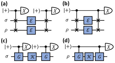
Figure 13: Different circuits for measuring the detector.

Since our channel purification protocol also only focuses on improving the channel rather than placing restrictions on the incoming and output state, it is natural for us to use the coherent detector circuit to perform channel purification as we have outlined before. If we indeed try to use the incoherent detector circuit for channel purification, the symmetrisation of the input state means that we have $\frac{1}{2}\left(\rho\otimes\sigma+\sigma\otimes\rho\right)$ as output state instead. Hence, when it comes to the measurement stage, the only way to perform $O$ measurement on $\rho$ is by performing $O$ measurement on both of the registers since they both have $\rho$ components, or by having $\sigma=\rho$. Both of these cases can be challenging in choosing the ancillary state and measurement $\sigma$ and $S$ in order to fulfil the channel purification condition in Eq. 10 as will be explained later. This is why we focus on using the coherent detector to perform channel purification in this paper.

G.2 Property of involution operators

For a given involution operator $G$ (square to $I$), we can decompose any operator $A$ into components that commute and anti-commute with $G$:

$$A=A_{+}+A_{-}$$ (58)

with

$$A_{\pm}=\frac{A\pm GAG}{2}.$$

It is easy to see that $GA_{\pm}=\pm A_{\pm}G$.

Further defining the projection operators

$$\Pi_{\pm}=\frac{\mathbb{I}\pm G}{2},$$

in this way, we can obtain the components of $A$ that are in the $\pm 1$ eigensubspace of $G$ via:

$$\begin{split}\Pi_{\pm}A\Pi_{\pm}=\Pi_{\pm}A_{+}\Pi_{\pm}=\Pi_{\pm}A_{+}=A_{+}\Pi_{\pm}\end{split}$$ (59)

Note that $\Pi_{\pm}A\Pi_{\pm}\neq A_{\pm}$. $A_{\pm}$ are components in $A$ that gain a $\pm 1$ factor when conjugated with $G$, while $\Pi_{\pm}A\Pi_{\pm}$ are components that get an $\pm 1$ factor when acted by $G$ on either side.

For the components of $A$ that connect between the $\pm 1$ eigensubspaces of $G$, we have:

$$\begin{split}\Pi_{\pm}A\Pi_{\mp}=\Pi_{\pm}A_{-}\Pi_{\mp}=\Pi_{\pm}A_{-}=A_{-}\Pi_{\mp}\end{split}$$ (60)

We can rewrite $A$ as

$$A =\underbrace{\Pi_{+}A\Pi_{+}+\Pi_{-}A\Pi_{-}}_{A_{+}}+\underbrace{\Pi_{+}A\Pi_{-}+\Pi_{-}A\Pi_{+}}_{A_{-}}$$

$$=\underbrace{\Pi_{+}A_{+}\Pi_{+}+\Pi_{-}A_{+}\Pi_{-}}_{A_{+}}+\underbrace{\Pi_{+}A_{-}\Pi_{-}+\Pi_{-}A_{-}\Pi_{+}}_{A_{-}}$$

where we see that $A_{+}$ contains the components of $A$ in both of the $\pm 1$ eigenspace, while $A_{+}$ contains the components of $A$ that represent the transition between the two eigensubspaces.

G.3 Coherent detector

For the noise channel $\mathcal{K}(\rho)=\sum_{i}K_{i}\rho K_{i}^{\dagger}$, each Kraus element can be decomposed into $K_{i}=K_{i,+}+K_{i,-}$ as discussed in Eq. 58.

When post-selecting on $\ket{\pm}$ output on the control qubit of Fig. 13(d), the output state is given as:

$$\mathcal{K}_{\mathrm{coh}}^{\pm}(\rho) =\frac{1}{4}\sum_{i}\bigg{[}\left(K_{i,+}+K_{i,-}\right)\rho\left(K_{i,+}^{\dagger}+K_{i,-}^{\dagger}\right)$$

$$\quad+\left(K_{i,+}-K_{i,-}\right)\rho\left(K_{i,+}^{\dagger}-K_{i,-}^{\dagger}\right)$$

$$\quad\pm\left(K_{i,+}+K_{i,-}\right)\rho\left(K_{i,+}^{\dagger}-K_{i,-}^{\dagger}\right)$$

$$\quad\pm\left(K_{i,+}-K_{i,-}\right)\rho\left(K_{i,+}^{\dagger}+K_{i,-}^{\dagger}\right)\bigg{]}$$

$$=\sum_{i}K_{i,\pm}\rho K_{i,\pm}^{\dagger}$$ (61)

i.e. when for $+1$ outcome, we have removed the noise components that anticommute with $G$, and for $-1$ outcome, we have removed the noise components that commute with $G$. Note that $\mathbb{I}$ commutes with $G$, thus if we want to keep the identity component, we need to keep the $+1$ outcome.

Note that the coherent detector only removes the noise components of the wrong symmetry in $\mathcal{K}$ (make it invariant under conjugation of $G$). It does not enforce symmetry on the incoming state $\rho$ and also does not enforce symmetry on the output state.

G.4 Incoherent detector

Instead of performing the detector check coherently using one control qubit, we can also perform it incoherently using Fig. 13(c) and keep only the output for which the two consecutive control qubit measurement is consistent (i.e. their collective parity is even). In this case, using Eq. 59, the output state is given as:

$$\mathcal{K}_{\mathrm{inc}}^{\mathrm{even},\pm}(\rho) =\sum_{i}\Pi_{\pm}K_{i}\Pi_{\pm}\ \rho\ \Pi_{\pm}K_{i}^{\dagger}\Pi_{\pm}$$

$$=\sum_{i}\Pi_{\pm}K_{i,+}\left(\Pi_{\pm}\rho\Pi_{\pm}\right)K_{i,+}^{\dagger}\Pi_{\pm}$$

In this case, the anticommuting components in the noise operators $K_{i}$ are removed just like in the coherent detector case. However, on top of that, the input state and the output state are restricted to the $\pm 1$ eigensubspace of $G$.

It can be further written as:

$$\quad\mathcal{K}_{\mathrm{inc}}^{\mathrm{even},\pm}(\rho)=\sum_{i}K_{i,+}\ \rho_{+}\ K_{i,+}^{\dagger}\Pi_{\pm}$$

$$=\frac{1}{4}\big{[}\mathcal{K}_{\mathrm{coh}}^{+}(\rho)+\mathcal{K}_{\mathrm{coh}}^{+}(G\rho G)\pm\left(\mathcal{K}_{\mathrm{coh}}^{+}(\rho)+\mathcal{K}_{\mathrm{coh}}^{+}(G\rho G)\right)G\big{]}$$ (62)

which we can explicitly see that the coherent detector channel is just one of its components.

Similarly, the output of a circuit in Fig. 13, with the collective parity of the two measurements being odd, is given as:

$$\mathcal{K}_{\mathrm{inc}}^{\mathrm{odd},\pm}(\rho)=\sum_{i}\Pi_{\pm}K_{i}\Pi_{\mp}\ \rho\ \Pi_{\mp}K_{i}^{\dagger}\Pi_{\pm}$$

$$=\sum_{i}\Pi_{\pm}K_{i,-}\left(\Pi_{\mp}\rho\Pi_{\mp}\right)K_{i,-}^{\dagger}\Pi_{\pm}$$

$$=\frac{1}{4}\big{[}\mathcal{K}_{\mathrm{coh}}^{-}(\rho)+\mathcal{K}_{\mathrm{coh}}^{-}(G\rho G)\pm\left(\mathcal{K}_{\mathrm{coh}}^{-}(\rho)+\mathcal{K}_{\mathrm{coh}}^{-}(G\rho G)\right)G\big{]}$$ (63)

G.5 Implication for virtual channel purification

In the case of virtual channel purification, we have:

$$G \Rightarrow\text{SWAP}$$

$$\rho \Rightarrow\sigma\otimes\rho$$

$$\mathcal{K} \Rightarrow\mathcal{E}\otimes\mathcal{E}$$

and the output state using the coherent detector using Sec. G.3 is:

$$\mathcal{K}_{\mathrm{coh}}^{\pm}(\sigma\otimes\rho) =\frac{1}{2}\sum_{i,j}\bigg{[}\left(K_{i}\otimes K_{j}\right)\left(\sigma\otimes\rho\right)\left(K_{i}^{\dagger}\otimes K_{j}^{\dagger}\right)$$

$$\quad\pm\left(K_{i}\otimes K_{j}\right)\left(\sigma\otimes\rho\right)\left(K_{j}^{\dagger}\otimes K_{i}^{\dagger}\right)\bigg{]}$$

Using the coherent detector circuit, we can obtain the state for virtual channel purification by combining the result of the $\pm$ outcome:

$$\mathcal{K}_{\mathrm{dis}}(\sigma\otimes\rho) =\mathcal{K}_{\mathrm{coh}}^{+}(\sigma\otimes\rho)-\mathcal{K}_{\mathrm{coh}}^{-}(\sigma\otimes\rho)$$

$$=\sum_{i,j}\left(K_{i}\otimes K_{j}\right)\left(\sigma\otimes\rho\right)\left(K_{j}^{\dagger}\otimes K_{i}^{\dagger}\right)$$

The output state using incoherent detector using Secs. G.4 and G.4 is:

$$\mathcal{K}_{\mathrm{inc}}^{\mathrm{even},\pm}(\sigma\otimes\rho) =\frac{1}{4}\big{(}\mathcal{K}_{\mathrm{coh}}^{+}(\sigma\otimes\rho)+\mathcal{K}_{\mathrm{coh}}^{+}(\rho\otimes\sigma)$$

$$\quad\pm\left(\mathcal{K}_{\mathrm{coh}}^{+}(\sigma\otimes\rho)+\mathcal{K}_{\mathrm{coh}}^{+}(\rho\otimes\sigma)\right)\text{SWAP}\big{)}$$

$$\mathcal{K}_{\mathrm{inc}}^{\mathrm{odd},\pm}(\sigma\otimes\rho) =\frac{1}{4}\big{(}\mathcal{K}_{\mathrm{coh}}^{-}(\sigma\otimes\rho)+\mathcal{K}_{\mathrm{coh}}^{-}(\rho\otimes\sigma)$$

$$\quad\pm\left(\mathcal{K}_{\mathrm{coh}}^{-}(\sigma\otimes\rho)+\mathcal{K}_{\mathrm{coh}}^{-}(\rho\otimes\sigma)\right)\text{SWAP}\big{)}$$

For the incoherent detector circuit, by adding the results with the same collective parity and using the even parity result to subtract the odd parity result, we have:

$$\mathcal{K}_{\mathrm{nodis}}(\sigma\otimes\rho) =\left(\mathcal{K}_{\mathrm{inc}}^{\mathrm{even},+}(\sigma\otimes\rho)+\mathcal{K}_{\mathrm{inc}}^{\mathrm{even},-}(\sigma\otimes\rho)\right)$$

$$\quad-\left(\mathcal{K}_{\mathrm{inc}}^{\mathrm{odd},-}(\sigma\otimes\rho)+\mathcal{K}_{\mathrm{inc}}^{\mathrm{odd},-}(\sigma\otimes\rho)\right)$$

$$=\frac{1}{2}\bigg{(}\mathcal{K}_{\mathrm{coh}}^{+}(\sigma\otimes\rho)+\mathcal{K}_{\mathrm{coh}}^{+}(\rho\otimes\sigma)$$

$$\quad-\mathcal{K}_{\mathrm{coh}}^{-}(\sigma\otimes\rho)-\mathcal{K}_{\mathrm{coh}}^{-}(\rho\otimes\sigma)\bigg{)}$$

$$=\frac{1}{2}\left(\mathcal{K}_{\mathrm{dis}}(\sigma\otimes\rho)+\mathcal{K}_{\mathrm{dis}}(\rho\otimes\sigma)\right)$$

This seems to be able to be used to purify the channel. However, it is a mixture of output states with $\rho$ in the main register and also $\rho$ in the ancillary register, and this mixture cannot be separated by the control qubit measurement results. Hence, if we measure $O$ on one of the qubits, part of the time, it will measure on the $\sigma$ ancillary state, which is not our targeted result.

In order to perform channel purification using the incoherent detector circuit. There are two possible solutions:

• Choose the ancillary state to be $\rho$ and try to identify an ancillary measurement that satisfy Eq. 36.

• Fixed the ancillary measurement to be $O$ and try to identify an ancillary input state that satisfy Eq. 36.

Both of these are not trivial to perform and we will leave it for future investigation.

References

- Cai et al. [2023a] Z. Cai, R. Babbush, S. C. Benjamin, S. Endo, W. J. Huggins, Y. Li, J. R. McClean, and T. E. O’Brien, Quantum error mitigation, Rev. Mod. Phys. 95, 045005 (2023a).
- Google Quantum AI and Collaborators [2020] Google Quantum AI and Collaborators, Hartree-Fock on a superconducting qubit quantum computer, Science 369, 1084 (2020).
- Google Quantum AI and Collaborators [2022] Google Quantum AI and Collaborators, Formation of robust bound states of interacting microwave photons, Nature 612, 240 (2022).
- Kim et al. [2023] Y. Kim, A. Eddins, S. Anand, K. X. Wei, E. van den Berg, S. Rosenblatt, H. Nayfeh, Y. Wu, M. Zaletel, K. Temme, and A. Kandala, Evidence for the utility of quantum computing before fault tolerance, Nature 618, 500 (2023).
- Temme et al. [2017] K. Temme, S. Bravyi, and J. M. Gambetta, Error Mitigation for Short-Depth Quantum Circuits, Phys. Rev. Lett. 119, 180509 (2017).
- Endo et al. [2018] S. Endo, S. C. Benjamin, and Y. Li, Practical Quantum Error Mitigation for Near-Future Applications, Phys. Rev. X 8, 031027 (2018).
- Li and Benjamin [2017] Y. Li and S. C. Benjamin, Efficient Variational Quantum Simulator Incorporating Active Error Minimization, Phys. Rev. X 7, 021050 (2017).
- Huggins et al. [2021a] W. J. Huggins, S. McArdle, T. E. O’Brien, J. Lee, N. C. Rubin, S. Boixo, K. B. Whaley, R. Babbush, and J. R. McClean, Virtual Distillation for Quantum Error Mitigation, Phys. Rev. X 11, 041036 (2021a).
- Koczor [2021a] B. Koczor, Exponential Error Suppression for Near-Term Quantum Devices, Phys. Rev. X 11, 031057 (2021a).
- McArdle et al. [2019] S. McArdle, X. Yuan, and S. Benjamin, Error-Mitigated Digital Quantum Simulation, Phys. Rev. Lett. 122, 180501 (2019).
- Bonet-Monroig et al. [2018] X. Bonet-Monroig, R. Sagastizabal, M. Singh, and T. E. O’Brien, Low-cost error mitigation by symmetry verification, Phys. Rev. A 98, 062339 (2018).
- McClean et al. [2017] J. R. McClean, M. E. Kimchi-Schwartz, J. Carter, and W. A. de Jong, Hybrid quantum-classical hierarchy for mitigation of decoherence and determination of excited states, Phys. Rev. A 95, 042308 (2017).
- Koczor [2021b] B. Koczor, The dominant eigenvector of a noisy quantum state, New J. Phys. 23, 123047 (2021b).
- Dalzell et al. [2021] A. M. Dalzell, N. Hunter-Jones, and F. G. S. L. Brandão, Random quantum circuits transform local noise into global white noise, arXiv:2111.14907 [quant-ph] (2021).
- Bennett et al. [1996a] C. H. Bennett, G. Brassard, S. Popescu, B. Schumacher, J. A. Smolin, and W. K. Wootters, Purification of Noisy Entanglement and Faithful Teleportation via Noisy Channels, Phys. Rev. Lett. 76, 722 (1996a).
- Bennett et al. [1996b] C. H. Bennett, D. P. DiVincenzo, J. A. Smolin, and W. K. Wootters, Mixed-state entanglement and quantum error correction, Phys. Rev. A 54, 3824 (1996b).
- Cai and Benjamin [2019] Z. Cai and S. C. Benjamin, Constructing Smaller Pauli Twirling Sets for Arbitrary Error Channels, Sci Rep 9, 1 (2019).
- Wallman and Emerson [2016] J. J. Wallman and J. Emerson, Noise tailoring for scalable quantum computation via randomized compiling, Phys. Rev. A 94, 052325 (2016).
- Chao and Reichardt [2018] R. Chao and B. W. Reichardt, Quantum Error Correction with Only Two Extra Qubits, Phys. Rev. Lett. 121, 050502 (2018).
- Suzuki et al. [2022] Y. Suzuki, S. Endo, K. Fujii, and Y. Tokunaga, Quantum Error Mitigation as a Universal Error Reduction Technique: Applications from the NISQ to the Fault-Tolerant Quantum Computing Eras, PRX Quantum 3, 010345 (2022).
- Lostaglio and Ciani [2021] M. Lostaglio and A. Ciani, Error Mitigation and Quantum-Assisted Simulation in the Error Corrected Regime, Phys. Rev. Lett. 127, 200506 (2021).
- Piveteau et al. [2021] C. Piveteau, D. Sutter, S. Bravyi, J. M. Gambetta, and K. Temme, Error Mitigation for Universal Gates on Encoded Qubits, Phys. Rev. Lett. 127, 200505 (2021).
- Knill and Laflamme [1997] E. Knill and R. Laflamme, Theory of quantum error-correcting codes, Phys. Rev. A 55, 900 (1997).
- Bridgeman and Chubb [2017] J. C. Bridgeman and C. T. Chubb, Hand-waving and interpretive dance: An introductory course on tensor networks, Journal of Physics A: Mathematical and Theoretical 50, 223001 (2017).
- Chao and Reichardt [2020] R. Chao and B. W. Reichardt, Flag Fault-Tolerant Error Correction for any Stabilizer Code, PRX Quantum 1, 010302 (2020).
- Delfosse and Paetznick [2023] N. Delfosse and A. Paetznick, Spacetime codes of Clifford circuits, arXiv:2304.05943 [quant-ph] (2023).
- McEwen et al. [2023] M. McEwen, D. Bacon, and C. Gidney, Relaxing Hardware Requirements for Surface Code Circuits using Time-dynamics, Quantum 7, 1172 (2023).
- Huggins et al. [2021b] W. J. Huggins, J. R. McClean, N. C. Rubin, Z. Jiang, N. Wiebe, K. B. Whaley, and R. Babbush, Efficient and noise resilient measurements for quantum chemistry on near-term quantum computers, npj Quantum Information 7, 23 (2021b).
- Barenco et al. [1997] A. Barenco, A. Berthiaume, D. Deutsch, A. Ekert, R. Jozsa, and C. Macchiavello, Stabilization of Quantum Computations by Symmetrization, SIAM J. Comput. 26, 1541 (1997).
- Chiribella et al. [2013] G. Chiribella, G. M. D’Ariano, P. Perinotti, and B. Valiron, Quantum computations without definite causal structure, Phys. Rev. A 88, 022318 (2013).
- Lee et al. [2023] G. Lee, C. T. Hann, S. Puri, S. M. Girvin, and L. Jiang, Error Suppression for Arbitrary-Size Black Box Quantum Operations, Phys. Rev. Lett. 131, 190601 (2023).
- Miguel-Ramiro et al. [2023] J. Miguel-Ramiro, Z. Shi, L. Dellantonio, A. Chan, C. A. Muschik, and W. Dür, Superposed Quantum Error Mitigation, Phys. Rev. Lett. 131, 230601 (2023).
- Foldager and Koczor [2023] J. Foldager and B. Koczor, Can shallow quantum circuits scramble local noise into global white noise?, J. Phys. A: Math. Theor. 57, 015306 (2023).
- Hakoshima et al. [2023] H. Hakoshima, S. Endo, K. Yamamoto, Y. Matsuzaki, and N. Yoshioka, Localized Virtual Purification, arXiv:2308.13500 [quant-ph] (2023).
- Smolin and DiVincenzo [1996] J. A. Smolin and D. P. DiVincenzo, Five two-bit quantum gates are sufficient to implement the quantum Fredkin gate, Phys. Rev. A 53, 2855 (1996).
- Kim et al. [2022] Y. Kim, A. Morvan, L. B. Nguyen, R. K. Naik, C. Jünger, L. Chen, J. M. Kreikebaum, D. I. Santiago, and I. Siddiqi, High-fidelity three-qubit iToffoli gate for fixed-frequency superconducting qubits, Nat. Phys. 18, 783 (2022).
- Chapman et al. [2023] B. J. Chapman, S. J. de Graaf, S. H. Xue, Y. Zhang, J. Teoh, J. C. Curtis, T. Tsunoda, A. Eickbusch, A. P. Read, A. Koottandavida, S. O. Mundhada, L. Frunzio, M. Devoret, S. Girvin, and R. Schoelkopf, High-On-Off-Ratio Beam-Splitter Interaction for Gates on Bosonically Encoded Qubits, PRX Quantum 4, 020355 (2023).
- Cai et al. [2023b] Z. Cai, A. Siegel, and S. Benjamin, Looped Pipelines Enabling Effective 3D Qubit Lattices in a Strictly 2D Device, PRX Quantum 4, 020345 (2023b).
- Cai [2021a] Z. Cai, A Practical Framework for Quantum Error Mitigation, arXiv:2110.05389 [quant-ph] (2021a).
- O’Brien et al. [2021] T. E. O’Brien, S. Polla, N. C. Rubin, W. J. Huggins, S. McArdle, S. Boixo, J. R. McClean, and R. Babbush, Error Mitigation via Verified Phase Estimation, PRX Quantum 2, 020317 (2021).
- Huo and Li [2022] M. Huo and Y. Li, Dual-state purification for practical quantum error mitigation, Phys. Rev. A 105, 022427 (2022).
- Cai [2021b] Z. Cai, Resource-efficient Purification-based Quantum Error Mitigation, arXiv:2107.07279 [quant-ph] (2021b).
- McClean et al. [2020] J. R. McClean, Z. Jiang, N. C. Rubin, R. Babbush, and H. Neven, Decoding quantum errors with subspace expansions, Nature Communications 11, 636 (2020).
- Gottesman [2022] D. Gottesman, Opportunities and Challenges in Fault-Tolerant Quantum Computation, arXiv:2210.15844 [quant-ph] (2022).
- Cai [2021c] Z. Cai, Quantum Error Mitigation using Symmetry Expansion, Quantum 5, 548 (2021c).
- Yoshioka et al. [2022] N. Yoshioka, H. Hakoshima, Y. Matsuzaki, Y. Tokunaga, Y. Suzuki, and S. Endo, Generalized Quantum Subspace Expansion, Phys. Rev. Lett. 129, 020502 (2022).
- Gisin et al. [2005] N. Gisin, N. Linden, S. Massar, and S. Popescu, Error filtration and entanglement purification for quantum communication, Phys. Rev. A 72, 012338 (2005).
- Azuma et al. [2021] K. Azuma, S. Bäuml, T. Coopmans, D. Elkouss, and B. Li, Tools for quantum network design, AVS Quantum Science 3, 014101 (2021).
- Ecker et al. [2021] S. Ecker, P. Sohr, L. Bulla, M. Huber, M. Bohmann, and R. Ursin, Experimental Single-Copy Entanglement Distillation, Phys. Rev. Lett. 127, 040506 (2021).
- Childs et al. [2023] A. M. Childs, H. Fu, D. Leung, Z. Li, M. Ozols, and V. Vyas, Streaming quantum state purification, arXiv:2309.16387 [quant-ph] (2023).
- Devetak et al. [2004] I. Devetak, A. W. Harrow, and A. Winter, A Family of Quantum Protocols, Phys. Rev. Lett. 93, 230504 (2004).
- Devetak et al. [2008] I. Devetak, A. W. Harrow, and A. J. Winter, A Resource Framework for Quantum Shannon Theory, IEEE Transactions on Information Theory 54, 4587 (2008).
- Horodecki et al. [2003] M. Horodecki, P. W. Shor, and M. B. Ruskai, Entanglement Breaking Channels, Rev. Math. Phys. 15, 629 (2003).
- Schumacher and Nielsen [1996] B. Schumacher and M. A. Nielsen, Quantum data processing and error correction, Phys. Rev. A 54, 2629 (1996).
- Devetak [2005] I. Devetak, The Private Classical Capacity and Quantum Capacity of a Quantum Channel, IEEE Trans. Inform. Theory 51, 44 (2005).
- Minář et al. [2008] J. Minář, H. de Riedmatten, C. Simon, H. Zbinden, and N. Gisin, Phase-noise measurements in long-fiber interferometers for quantum-repeater applications, Phys. Rev. A 77, 052325 (2008).
- Vijayan et al. [2020] M. K. Vijayan, A. P. Lund, and P. P. Rohde, A robust W-state encoding for linear quantum optics, Quantum 4, 303 (2020).
- Chiribella and Kristjánsson [2019] G. Chiribella and H. Kristjánsson, Quantum Shannon theory with superpositions of trajectories, Proceedings of the Royal Society A: Mathematical, Physical and Engineering Sciences 475, 20180903 (2019).
- Abbott et al. [2020] A. A. Abbott, J. Wechs, D. Horsman, M. Mhalla, and C. Branciard, Communication through coherent control of quantum channels, Quantum 4, 333 (2020).
- Kristjánsson et al. [2023] H. Kristjánsson, Y. Zhong, A. Munson, and G. Chiribella, Quantum networks with coherent routing of information through multiple nodes, arXiv:2208.00480 [quant-ph] (2023).
- Takagi et al. [2023] R. Takagi, H. Tajima, and M. Gu, Universal Sampling Lower Bounds for Quantum Error Mitigation, Phys. Rev. Lett. 131, 210602 (2023).
- Tsubouchi et al. [2023] K. Tsubouchi, T. Sagawa, and N. Yoshioka, Universal Cost Bound of Quantum Error Mitigation Based on Quantum Estimation Theory, Phys. Rev. Lett. 131, 210601 (2023).
- Quek et al. [2022] Y. Quek, D. S. França, S. Khatri, J. J. Meyer, and J. Eisert, Exponentially tighter bounds on limitations of quantum error mitigation, arXiv:2210.11505 [math-ph, physics:quant-ph] (2022).
- Graydon et al. [2022] M. A. Graydon, J. Skanes-Norman, and J. J. Wallman, Designing Stochastic Channels, arXiv:2201.07156 [quant-ph] (2022).
- Carignan-Dugas et al. [2019] A. Carignan-Dugas, M. Alexander, and J. Emerson, A polar decomposition for quantum channels (with applications to bounding error propagation in quantum circuits), Quantum 3, 173 (2019).