revtex4-1Repair the float
Stabilizer entropy of quantum tetrahedra
Abstract
How complex is the structure of quantum geometry? In several approaches, the spacetime atoms are obtained by the intertwiner called quantum tetrahedron. The complexity of this construction has a concrete consequence in recent efforts to simulate such models and toward experimental demonstrations of quantum gravity effects. There are, therefore, both a computational and an experimental complexity inherent to this class of models. In this paper, we study this complexity under the lens of Stabilizer Entropy (SE). We calculate the SE of the gauge-invariant basis states and its average in the gauge invariant subspace. We find that the states of definite volume are singled out by the (near) maximal SE and give precise bounds to the verification protocols for experimental demonstrations on available quantum computers.
I Introduction
Understanding whether gravity admits a quantum formulation is one of the most intriguing challenges of modern physics. In the last decade, quantum information theory has provided new conceptual and mathematical tools to investigate the structure of spacetime at the quantum scale. Entanglement entropy has been used to probe the holographic architecture of spacetime, supporting the idea of entanglement as an essential resource to the emergence of classical spacetime geometry [1, 2, 3, 4, 5]. Recently, also fostered by new perspectives in quantum gravity phenomenology, the use of quantum information tools to design and investigate experimental evidence for quantum features of the gravitational field has attracted much attention [8, 9, 10].
Within the limits of current experimental technology, the first widely available quantum computers today allow to simulate quantum gravity states, providing suggestions, predictions and setup ideas for future experiments [11, 12, 13]. In this scenario, we expect non-stabilizer resources to play a double key role. Gently speaking, non-stabilizerness is a core property of quantum states describing the complexity of the expression of their density operator in a specific operator basis (in the case of qubit systems, the Pauli operator basis), and its interplay with entanglement is known to be the essential ingredient needed to unlock quantum advantage [14, 15]. Recently, this resource has been shown to be given an entropic meaning, as Stabilizer Entropy (SE), making it both computable [16] and measurable [17]. SE directly affects the cost (in terms of classical resources) of simulating a quantum state or process: a -qubit state or circuit using a number of non-stabilizer resources can be simulated with a classical computer at a computational cost that scales as [18]. In particular, it provides bounds on the fidelity reachable in experimental realizations of quantum states [19]. Moreover, SE is involved in the onset of universal, complex patterns of entanglement [20, 21], quantum chaos [22, 23, 24, 25], complexity in the wave function of quantum many-body systems [26, 27], and decoding algorithms from black hole’s Hawking radiation [28, 29, 30, 31]. States and processes with high non-stabilizer resources are generically exponentially harder to simulate on a classical computer, and they are harder to certificate in experimental protocols. An analysis of such resources is therefore vital in order to assess the simulability of quantum gravity states. At the same time, we expect such property to provide a new tool, in addition to entanglement, to investigate the emergence of classical spacetime in quantum gravity.
In this work, we explore the novel direction of looking at the non-stabilizerness of quantum gravity states in the setting of non-perturbative theories. We consider a description of quantum geometry given in terms of spin network states, a general tool shared by lattice gauge theory [32] and several background-independent approaches to quantum gravity (like loop quantum gravity [33, 34], state sum models [35, 36], and group field theories [37, 38, 39]), where they provide a gauge-invariant basis for the field. A spin network is represented by a graph , with edges and nodes colored respectively by spin halves and intertwiner operators [34].
Each node of the network graph is dual to a quantum polyhedron geometry, with a number of faces equal to the valence of the node. We focus on a single valent node, that is an -gauge invariant state corresponding to a quantum tetrahedron [40, 41, 42, 43].
We study the non-stabilizerness of quantum tetrahedron states using Stabilizer Entropy (SE) [16]. The first result of the work is that the states that diagonalize the oriented volume operator are the ones with highest value of SE: this result provides a new lower bound for the number of preparations needed in future experimental setups of quantum gravity states. To our knowledge, at present, this bound, obtained from the calculated intertwiner states non-stabilizerness has not been fully reached yet (see e.g. the data from the experiments realized in [11]). As a second result, we show that the projection into the gauge invariant Hilbert space associated to the process of constructing the quantum tetrahedron out of a collection of four qubits inherently requires non-stabilizer resources. Such resources become an intrinsic feature of the quantum geometry state, reflecting in the computational complexity of a simulation of such processes, in a way that is ultimately dependent on the structure of the gauge invariant space itself.
The paper is organized as follows. Section II provides the basic notions of the stabilizer formalism necessary for our analysis. We recall the definition of Pauli operators, the Clifford group and construct the set of pure stabilizer states, highlighting the necessity to go beyond this set of states in order to unlock quantum advantage. Then, we introduce the definition of Stabilizer Entropy as an entropic measure of nonstabilizerness of a pure quantum state, as well as its properties. In Section III we introduce the setting of quantum gravity. We realize a quantum tetrahedron via projection into the SU gauge invariant (intertwiner) subspace of a spin network Hilbert space. We show the most general intertwiner state for any SU spin irrep and then focus on the case of . In Section IV and Section VI we compute the non-stabilizerness of the logical basis and of the volume eigenstates basis elements. Then, these numerical results provide an estimate of the upper bound of the fidelity of the experiment in [11]; we compare our estimations with the experimental fidelity obtained. In Section V we extend the analysis to non-stabilizerness of subspaces, in order to investigate the cost of projection in terms of non-stabilizer resources. To this end, we introduce the average SE gap onto a subspace, and we show that this quantity is directly dependent from the internal structure of said subspace in the form of its projector. Finally, we apply our obtained results to the intertwiner subspace and conclude that imposing the gauge invariance has an intrinsic cost in terms of non-stabilizer resources.
II Stabilizer formalism and Stabilizer Entropy
In this section, we review the stabilizer formalism and its role in the quantum computation framework.
Let a -qubit system and be the Pauli group acting on . Define the Clifford group as the normalizer of the Pauli group, namely, [44]. Hence, given a computational basis of as the common eigenbasis of the operators belonging to , one can define the set of pure stabilizer states of as the full Clifford orbit of [45], namely
| (1) |
Stabilizer states share some properties with regard to the computational complexity of simulating quantum processes using classical resources; these properties are summarized by the Gottesman-Knill theorem, which states that any quantum process that can be represented with initial stabilizer states upon which one performs (i) Clifford unitaries, (ii) measurements of Pauli operators, (iii) Clifford operations conditioned on classical randomness, can be perfectly simulated by a classical computer in polynomial time [44]. This means that stabilizer states and Clifford operators are not actually “quantum" from a computational perspective, since they do not provide any advantage over classical computers. Since the set of stabilizer states is by definition closed under Clifford operations, a certain amount of resources beyond the Clifford group is needed to prepare a generic state in the Hilbert space: this quantity is referred to as non-stabilizerness of this state, which has been proven to be a useful resource for universal quantum computation [46] and for which several measures have been proposed [47, 45]. For our analysis, we are going to use two entropic non-stabilizerness measures called 2-Stabilizer Rényi Entropy (SE) [16] and its linear counterpart. They are defined starting from the probability distribution , with and , associated to the tomography of the quantum state . Then, the -Stabilizer Rényi Entropy for pure states is defined as
| (2) |
whereas the linear SE is defined as
| (3) |
Both and are: (i) faithful, i.e. , otherwise ; (ii) invariant under Clifford operators, namely , whereas is also additive under tensor product of quantum states [16]. Both measures can also be written in a more compact form:
| (4) |
with . This construction can be generalized in a straightforward way to the Pauli group (namely, the Heisenberg-Weyl group) for qudits, that is, level systems [48], and the SE are defined exactly as in Eq.(4), see Appendix C for details.
Stabilizer entropies quantify the computational complexity of qubit states by the entropy of the distribution over the Pauli basis: states with high values of or require an exponential amount of classical resources to be simulated, and hence are those which may exhibit quantum advantage.
Moreover, a result shown in [19] establishes a bound between SE and minimum number of copies needed to achieve a certain fidelity in certification protocols: therefore, from a computational perspective, the knowledge of SE of quantum gravity states is an essential tool to optimize time and resources involved in the preparation of the states on a quantum computer, once a desired value of fidelity has been established.
III Quantum tetrahedron
Spin networks are symmetric tensor network states defined by a graphs , labeled by SU irreducible representations and intertwining operators. In loop quantum gravity, such states encode the quantum description of the 3D space manifold into purely combinatorial and algebraic variables [49, 50]. More generally, spin networks can be defined as abstract quantum many-body-like collections of fundamental quanta of space, connected by maximally entangled states to describe quantized discrete spatial geometries [39, 51, 52].
Consider a given graph . To each edge of we associate a half-integer spin variable labeling a -dimensional irreducible representation space . At the same time, each -valent node carries an intertwiner state in the -invariant Hilbert space , which is the degeneracy space associated to the recoupling of the spins meeting at the node into a singlet (gauge invariant) representation. A spin-network basis state is the triple , defined by the direct sum over of the tensor product of the gauge invariant states at all nodes:
| (5) |
Spin network states can be enriched with a geometric interpretation: each -valent node is dual to a -simplex, represented at the quantum level by the intertwiner state. Accordingly, a 4-valent intertwiner state describes the quantized geometry of a 3-simplex, namely a quantum tetrahedron [53, 54]. In the context of LQG, the presence of clearly defined geometric operators, such as the area operator and the volume operator [49, 43], further strengthens the geometric interpretation; in particular, the volume operator acting on a valent node is given by
| (6) |
and has a diagonal representation on the intertwiner basis [55]. Note that this operator is Hermitian but not positive, since it also keeps information of the space orientation [36]. The two possible signs split the degeneracy between the eigenvalues.
For the sake of our work, we focus on the case of a single 4-valent intertwiner with all spins fixed to the same value . The Hilbert space of the tensor product of the four spins recoupling into the total spin can be written as
| (7) |
where the multiplicity spaces (or degeneracy spaces) consist in the spaces of -invariant intetrtwiner states in the tensor product of the total spin Hilbert space with the individual spins .
A state can be written as the recoupling of four spins into the singlet ():
| (8) |
where is a normalization factor and are the Clebsch-Gordan coefficients involved in the intermediate recoupling of the two pairs of spins into two states with spin ; to ensure the final recoupling into a singlet state, the magnetic indices have opposite signs. We use the shorthand notation to indicate the sum running over the basis element in . In the following, we set all spins to the value (see Appendix C for a short discussion on the case ). In this case, the spin representation space reduces to , therefore, each spin, which is dual to one of the faces of the tetrahedron, is described by a qubit. The Hilbert space of the tensor product of the four -spins decomposes as
| (9) |
The -invariant subspace comes with degeneracy , hence any gauge invariant state is a one qubit state in the 2-dimensional intertwiner Hilbert space
| (10) |
where we can choose a suitable basis . We can represent a 4-valent intertwiner state both in the computational basis of the 4-qubits space and in the logical basis . In the following we will refer to a state written in the logical basis as a logical intertwiner qubit (LIQ) state [56].
In terms of the computational basis, the expression of the elements of logical basis can be found using (8). Explicitly, one finds [57, 11]:
| (11) |
A generic LIQ state is given by the following Bloch representation
| (12) |
where and are angles on the Bloch sphere. Finally, it can be shown [11] that the eigenstates of the volume operator take the following form:
| (13) | ||||
| (14) |
that means . These states represent remarkable points on the Bloch sphere, as they are placed at the equator and their angular coordinates are and .
IV Stabilizer entropy of a quantum tetrahedron
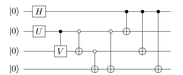
We shall investigate whether the basis states of the gauge invariant subspace possess SE. In this sense, we investigate whether the gates of the quantum circuit associated with the construction of LIQ states from the computational basis belong to the Clifford group. Without loss of generality, we can start from the reference state , and then look for unitary transformations such that and . Using the relations in Eq. 11, we can express the unitary operators and in terms of a set of unitary gates acting on a stabilizer reference state in the 4-qubit Hilbert space. Thereby, it is possible to realize the generic intertwiner state via the quantum circuit given in Fig. 1 [11] (see also [58] and [59, 60] for different descriptions of quantum spin network circuits). The only non-Clifford gates in the circuit are the two special unitary operators, and , which depend on the parameters and of the output state .
Such operators can be written as matrices [11]:
| (15) |
| (16) |
where the coefficients and are given by the following functions of and :
| (17) | ||||
| (18) |
Our first remark is that the SE of an intertwiner state seen from the full space is entirely determined by the gates and , which in general are not Clifford gates. Indeed, the calculation of the SE for the LIQ basis states (see Appendix A for full details) gives
| (19) | ||||
Hence, a generic superposition of these two basis states will not be in general a stabilizer state. We can plot the SE of all the intertwiner states in the basis of the Hilbert space as a function of the Bloch sphere representation of the gauge invariant space (Fig. 2).
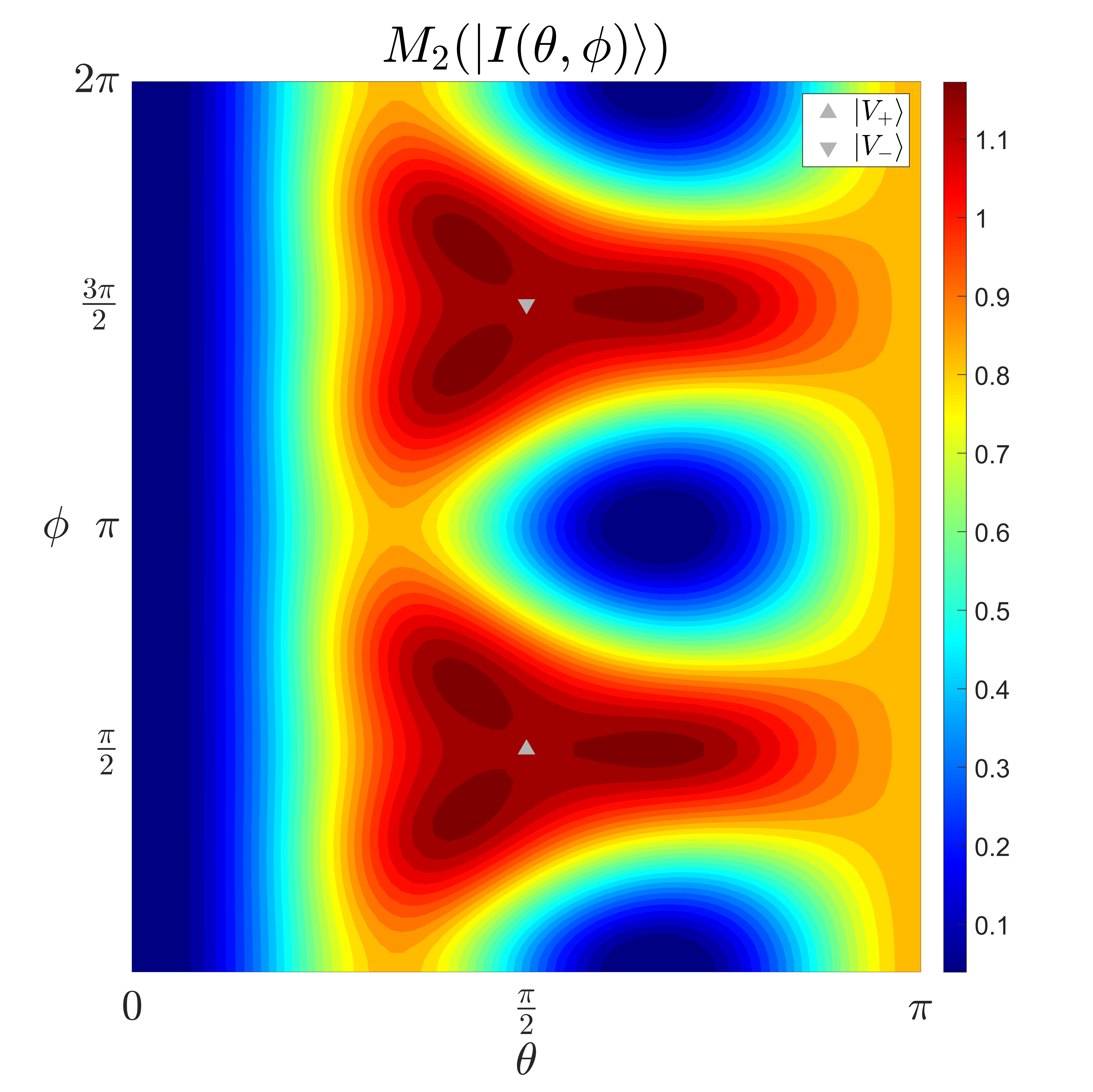
In particular, we remark the behavior of the volume eigenstates : from the SE standpoint, they are located at the center of the regions of maximal non-stabilizerness and they belong to the same Clifford orbit, having exactly the same value of SE:
| (20) |
We recall that the SE of these states is calculated with respect to the full Pauli operator basis of , namely the Pauli group of -qubits . This distinction is necessary since, as we have seen in Eq. (19), the basis states themselves are not stabilizer states in , whereas they are stabilizers in . Finally, notice that these states are also non separable in the tensor product structure associated to , as a demonstration that both entanglement and SE are necessary for the gauge structure[61, 62, 63, 64].
V Average SE of -gauge invariant subspace
The reason for having different values of SE in the two bases states, as shown in Eq. (11), is rooted in the gauge structure of the intertwiner state. We shall explore and generalize this result further. The gauge invariant intertwiner space is a subspace of the Hilbert space of four qubits . However, the SE in a particular basis state has hardly any physical meaning as any superposition of states in is allowed and SE is not constant in any given subspace. To associate SE in a meaningful way to a subspace, one is also confronted with the choice of the Pauli basis with respect to the SE must be computed. To be concrete, if one has a state , do we want to know the SE of this state as a state expressed in the computational basis of or in the computational basis of given by ?
In the construction of a quantum gauge theory, one starts with an ambient Hilbert space . The gauge constraints are expressed as local projectors and the gauge invariant subspace is the global projection over all the local gauge constraints,
| (21) |
with .
We associate to a subspace its average SE with respect to the Heisenberg-Weyl basis . In this notation, refers to the Heisenberg-Weyl basis in , while refers to the gauge invariant Hilbert space . With this notation, the linear SE is and the operator
| (22) |
is defined accordingly with the corresponding Heisenberg-Weyl (see Appendix C for details) basis. The average SE in the subspace is then defined as
| (23) | |||||
| (24) |
with denoting the unitary group average with respect to the Haar measure over , and . In order to perform the Haar average over the subspace we need the following:
Lemma 1.
Given any Hilbert space , with and , the unitary Haar average of copies of the state over the subspace is given by
| (25) |
with , , the projector onto , and .
A proof of this lemma is given in Section B.2. Based on the above lemma, we obtain the general result
| (26) |
where now denotes the Haar average over the full unitary group on .
Eq.(26) shows explicitly how the gauge structure enters the SE through the projector . When , this projector becomes the identity map and the average SE has no recollection of the gauge structure. In order to quantify the amount of SE due to this structure, we define the SE-gap as
For a general gauge structure, namely the spin intertwiner states, the projector reads (see Appendix C)
| (28) |
Let us now specialize these formulae to the case of , that is, the quantum tetrahedron. Using Lemma 1, with , , and being the projector onto the intertwiner space, (see Appendix B for details) we find
| (29) |
Now, notice that the logical states in the Pauli basis in which are obviously stabilizer states with zero stabilizer entropy. Nevertheless even according to this Pauli basis there will be a non-zero value for the average stabilizer entropy. This space is just a generic qubit from the point of view of the stabilizer entropy. The average SE in this space is thus just the average stabilizer entropy of a qubit, namely , as calculated in [16] (we also explicitly show this calculation in Appendix B).
Putting the pieces together, we are able to calculate the average SE gap, which reads
| (30) |
A value of greater than zero tells us that projecting a generic -qubit state onto this gauge invariant subspace has a cost in terms of non-stabilizer resources.
In particular, this means that the gauge structure bears a cost in terms of simulability, which is very important as one scales the system to many nodes.
VI Simulations of quantum gravity states
Very recently, quantum gravity states have been physically implemented on quantum computers [11, 12], and in particular, quantum tetrahedra states. The very first layer of difficulty that must be faced in a laboratory when attempting to conduct a quantum experiment (including one regarding simulations of quantum gravity states) is the preparation of an initial state that is faithful to the theoretical one . Typically, a large initial sample must be prepared, resulting in a mixed output from the processor. Ensuring the correct functioning of quantum devices in terms of the accuracy of the output requires a certification protocol [65]; one of the possible measures of the quality of the realization of a state is the fidelity that measures the precision of preparation. It is known that SE can provide useful indications in an experimental setting.
In this last section, we argue that the numerical results found in (19) and (20) have a direct use in the recent results on quantum gravity states simulations. Indeed, we can use the SE of these states to estimate the maximum fidelity achievable with a given number of preparations or, conversely, the minimum number of preparations needed to achieve a desired value of fidelity within a desired error [19].
In [11], the authors present a realization of the intertwiner states as of Eq. (11) as well as the volume eigenstates on a -qubit (Yorktown) and a -qubit (Melbourne) IBM superconducting quantum computer. By performing 10 rounds of 1024 quantum measurements, they obtained fidelity values of the prepared states with respect to the theoretical ones. As anticipated in Sec. II, the explicit lower bound on the number of preparations needed to achieve an accuracy , with a probability of failure , is related to the SE of the theoretical state as follows:
| (31) |
Inverting this relation, one can get an upper bound on the maximum achievable fidelity with a given number of preparations with failure probability :
| (32) |
| 0,906 | 0,005 | 0 | 0,05 | 0,973 | 835 | |
| 0,916 | 0,007 | 0,847997 | 0,05 | 0,959 | 2441 | |
| 0,918 | 0,009 | 1,16993 | 0,05 | 0,952 | 3535 | |
| 0,917 | 0,008 | 1,16993 | 0,05 | 0,952 | 3450 |
As one can see from the Table 1, the experimentally obtained data for the the fidelity is perfectly compatible with the bounds provided by the SE. However, the authors used many more copies than the minimum shown in the table. However, it is important to note that the constraints provided by Eqs. (31) and (32) are purely theoretical, hence independent of the inherent noise sources peculiar to the specific implementation protocols and hardware used in the experimental setting at hand. Nevertheless, by considering the SE of the states one wishes to prepare, the hardware resources and the number of preparations can be managed more efficiently in future experiments of quantum gravity states.
VII Discussion
In this paper, we have shown that the gauge invariant structure of quantum geometry states has a cost in terms of non-stabilizer resources. This implies that simulations of quantum geometry states can run more efficiently on a quantum computer and that preparations of future experiments can be more efficient if the non-stabilizer property of the state is taken into account. Moreover, we have seen that eigenstates of the oriented volume have near-maximal amount of SE: this begs the question of why such states possess greater quantum complexity, suggesting that a correspondence between entanglement and geometry in quantum gravity may extend at a deeper layer of quantumness. Concretely, the first step to answer this question will be to repeat this analysis for a generic spin- intertwiner and see if, also in that setting, the volume eigenstates are states with maximum SE. A further intriguing direction to explore is the role of non-stabilizer resources when taking into account the quantum state associated to an actual spin network, that is a collection of intertwiners describing a quantum simplicial complex: in that general setting, one should expect additional non-stabilizer resources coming from the graph structure, that is the adjacency matrix, describing the connectivity and the non-trivial additional geometrical degrees of freedom described by the holonomies dressing the links. In particular, in this sense, we expect that non-stabilizerness can be further used to characterise the transition amplitudes, that is the evolution, of quantum geometry states (see e.g. [12]).
In general terms, the dependence of the SE gap from the projector onto the intertwiner subspace opens to more wide-reaching questions: how does the gauge structure affect non-stabilizerness in a more general setting? Can we use this formalism to characterize the SE of other quantum gauge theories? Does abelianity (or lack thereof) of the gauge group play a role in the non-stabilizer resources of the gauge invariant subspace?
VIII acknowledgments
The authors thank L. Leone and L. Vacchiano for important discussions. AH acknowledges support from the PNRR MUR project PE0000023-NQSTI and PNRR MUR project CN -ICSC.
References
- Ryu and Takayanagi [2006] S. Ryu and T. Takayanagi, Journal of High Energy Physics 2006, 045 (2006).
- Van Raamsdonk [2010] M. Van Raamsdonk, Gen. Rel. Grav. 42, 2323 (2010).
- Maldacena and Susskind [2013a] J. Maldacena and L. Susskind, Fortschritte der Physik 61, 781 (2013a).
- Bianchi and Myers [2014] E. Bianchi and R. C. Myers, Classical and Quantum Gravity 31, 214002 (2014).
- Cao et al. [2017] C. Cao, S. M. Carroll, and S. Michalakis, Phys. Rev. D 95, 024031 (2017).
- Maldacena and Susskind [2013b] J. Maldacena and L. Susskind, Fortschritte der Physik 61, 781 (2013b) .
- Susskind [2014] L. Susskind, “Entanglement is not enough,” (2014), arXiv:1411.0690 [hep-th] .
- Westphal et al. [2021] T. Westphal, H. Hepach, J. Pfaff, and M. Aspelmeyer, “Measurement of gravitational coupling between millimeter-sized masses,” (2021), arXiv:2009.09546 [gr-qc] .
- Overstreet et al. [2023] C. Overstreet, J. Curti, M. Kim, P. Asenbaum, M. A. Kasevich, and F. Giacomini, Physical Review D 108 (2023), 10.1103/physrevd.108.084038.
- Christodoulou et al. [2023] M. Christodoulou, A. D. Biagio, R. Howl, and C. Rovelli, Classical and Quantum Gravity 40, 047001 (2023).
- Czelusta and Mielczarek [2021] G. Czelusta and J. Mielczarek, Physical Review D 103 (2021), 10.1103/physrevd.103.046001.
- van der Meer et al. [2023] R. van der Meer, Z. Huang, M. C. Anguita, D. Qu, P. Hooijschuur, H. Liu, M. Han, J. J. Renema, and L. Cohen, npj Quantum Inf. 9, 32 (2023), arXiv:2207.00557 [quant-ph] .
- Polino et al. [2022] E. Polino, B. Polacchi, D. Poderini, I. Agresti, G. Carvacho, F. Sciarrino, A. D. Biagio, C. Rovelli, and M. Christodoulou, “Photonic implementation of quantum gravity simulator,” (2022), arXiv:2207.01680 [quant-ph] .
- Campbell et al. [2017] E. T. Campbell, B. M. Terhal, and C. Vuillot, Nature 549, 172–179 (2017).
- Tirrito et al. [2023] E. Tirrito, P. S. Tarabunga, G. Lami, T. Chanda, L. Leone, S. F. E. Oliviero, M. Dalmonte, M. Collura, and A. Hamma, “Quantifying non-stabilizerness through entanglement spectrum flatness,” (2023), arXiv:2304.01175 [quant-ph] .
- Leone et al. [2022a] L. Leone, S. F. E. Oliviero, and A. Hamma, Physical Review Letters 128, 050402 (2022a).
- Oliviero et al. [2022a] S. F. E. Oliviero, L. Leone, A. Hamma, and S. Lloyd, npj Quantum Inf. 8, 148 (2022a), arXiv:2204.00015 [quant-ph] .
- Aaronson and Gottesman [2004] S. Aaronson and D. Gottesman, Physical Review A 70, 052328 (2004).
- Leone et al. [2023] L. Leone, S. F. E. Oliviero, and A. Hamma, Phys. Rev. A 107, 022429 (2023).
- Piemontese et al. [2022] S. Piemontese, T. Roscilde, and A. Hamma, “Entanglement complexity of the Rokhsar-Kivelson-sign wavefunctions,” (2022), arXiv:2211.01428 [quant-ph] .
- True and Hamma [2022] S. True and A. Hamma, Quantum 6, 818 (2022).
- Leone et al. [2021a] L. Leone, S. F. E. Oliviero, and A. Hamma, Entropy 23 (2021a), 10.3390/e23081073.
- Oliviero et al. [2021a] S. F. E. Oliviero, L. Leone, F. Caravelli, and A. Hamma, SciPost Physics 10, 76 (2021a).
- Leone et al. [2021b] L. Leone, S. F. E. Oliviero, Y. Zhou, and A. Hamma, Quantum 5, 453 (2021b).
- Oliviero et al. [2021b] S. F. E. Oliviero, L. Leone, and A. Hamma, Physics Letters A 418, 127721 (2021b).
- Oliviero et al. [2022b] S. F. E. Oliviero, L. Leone, and A. Hamma, Phys. Rev. A 106, 042426 (2022b).
- Haug and Piroli [2023] T. Haug and L. Piroli, Phys. Rev. B 107, 035148 (2023).
- Leone et al. [2022b] L. Leone, S. F. E. Oliviero, S. Piemontese, S. True, and A. Hamma, Phys. Rev. A 106, 062434 (2022b).
- Oliviero et al. [2022c] S. F. E. Oliviero, L. Leone, S. Lloyd, and A. Hamma, “Black Hole complexity, unscrambling, and stabilizer thermal machines,” (2022c), arXiv:2212.11337 [gr-qc, physics:hep-th, physics:quant-ph] .
- Leone et al. [2022c] L. Leone, S. F. E. Oliviero, S. Lloyd, and A. Hamma, “Learning efficient decoders for quasi-chaotic quantum scramblers,” (2022c), arXiv:2212.11338 [quant-ph] .
- Hayden and Preskill [2007] P. Hayden and J. Preskill, Journal of High Energy Physics 2007, 120 (2007).
- Donnelly [2014] W. Donnelly, Classical and Quantum Gravity 31, 214003 (2014).
- Thiemann [2007] T. Thiemann, “Loop quantum gravity: An inside view,” in Lecture Notes in Physics (Springer Berlin Heidelberg, 2007) p. 185–263.
- Rovelli and Vidotto [2014] C. Rovelli and F. Vidotto, Covariant Loop Quantum Gravity: An Elementary Introduction to Quantum Gravity and Spinfoam Theory (Cambridge University Press, 2014).
- H. [1992] O. H., Mod. Phys. Lett. A 07, 2799 (1992).
- Baez and Barrett [1999] J. C. Baez and J. W. Barrett, “The quantum tetrahedron in 3 and 4 dimensions,” (1999), arXiv:gr-qc/9903060 [gr-qc] .
- Oriti [2007] D. Oriti, “The group field theory approach to quantum gravity,” (2007), arXiv:gr-qc/0607032 [gr-qc] .
- Oriti [2009] D. Oriti, “The group field theory approach to quantum gravity: some recent results,” (2009), arXiv:0912.2441 [hep-th] .
- Oriti [2015] D. Oriti, “Group field theory as the 2nd quantization of loop quantum gravity,” (2015), arXiv:1310.7786 [gr-qc] .
- Ponzano and Regge [1969] G. P. Ponzano and T. E. Regge (1969).
- Regge [1961] T. Regge, Nuovo Cim. 19, 558 (1961).
- Barbieri [1998a] A. Barbieri, Nuclear Physics B 518, 714 (1998a).
- Bianchi and Haggard [2011] E. Bianchi and H. M. Haggard, Phys. Rev. Lett. 107, 011301 (2011).
- Gottesman [1998] D. Gottesman, “The heisenberg representation of quantum computers,” (1998), arXiv:quant-ph/9807006 [quant-ph] .
- Veitch et al. [2014] V. Veitch, S. A. H. Mousavian, D. Gottesman, and J. Emerson, New Journal of Physics 16, 013009 (2014).
- Bravyi and Kitaev [2005] S. Bravyi and A. Kitaev, Physical Review A 71, 022316 (2005).
- Howard and Campbell [2017] M. Howard and E. Campbell, Physical Review Letters 118, 090501 (2017).
- Wang and Li [2023] Y. Wang and Y. Li, Quantum Information Processing 22, 444 (2023).
- Rovelli and Smolin [1995a] C. Rovelli and L. Smolin, Phys. Rev. D 52, 5743 (1995a).
- Freidel and Speziale [2010] L. Freidel and S. Speziale, Phys. Rev. D 82, 084040 (2010).
- Chirco et al. [2018] G. Chirco, D. Oriti, and M. Zhang, Class. Quant. Grav. 35, 115011 (2018).
- Colafranceschi et al. [2022] E. Colafranceschi, G. Chirco, and D. Oriti, Phys. Rev. D 105, 066005 (2022).
- Barbieri [1998b] A. Barbieri, Nuclear Physics B 518, 714 (1998b).
- Bianchi et al. [2011] E. Bianchi, P. Doná, and S. Speziale, Phys. Rev. D 83, 044035 (2011).
- Rovelli and Smolin [1995b] C. Rovelli and L. Smolin, Nuclear Physics B 442, 593–619 (1995b).
- Mielczarek [2018] J. Mielczarek, “Spin networks on adiabatic quantum computer,” (2018), arXiv:1801.06017 [gr-qc] .
- Feller and Livine [2016] A. Feller and E. R. Livine, Classical and Quantum Gravity 33, 065005 (2016).
- Girelli and Livine [2005] F. Girelli and E. R. Livine, Classical and Quantum Gravity 22, 3295 (2005).
- Marzuoli and Rasetti [2002] A. Marzuoli and M. Rasetti, Physics Letters A 306, 79 (2002).
- Marzuoli and Rasetti [2017] A. Marzuoli and M. Rasetti, International Journal of Circuit Theory and Applications 45, 951 (2017).
- Hamma et al. [2005] A. Hamma, R. Ionicioiu, and P. Zanardi, Phys. Rev. A 72, 012324 (2005).
- Ghosh et al. [2015] S. Ghosh, R. M. Soni, and S. P. Trivedi, JHEP 09, 069 (2015).
- Donnelly [2008] W. Donnelly, Phys. Rev. D 77, 104006 (2008).
- Schliemann [2005] J. Schliemann, Phys. Rev. A 72, 012307 (2005).
- Eisert et al. [2020] J. Eisert, D. Hangleiter, N. Walk, I. Roth, D. Markham, R. Parekh, U. Chabaud, and E. Kashefi, Nature Reviews Physics 2, 382–390 (2020).
- Roberts and Yoshida [2017] D. A. Roberts and B. Yoshida, Journal of High Energy Physics 2017, 121 (2017).
Appendix A Calculation of the SE of the intertwiner basis states
In this section, we show the details of the calculations of the SE of the intertwiner basis state, namely the south and north poles of the Bloch sphere (i.e. and ). Recalling the circuit realization of the intertwiner states in (Fig. 1), we focus on the unitary operators , , , involved in the preparation of basis states and , which can be calculated by inserting in Eq. 17 and , respectively:
| (37) | ||||
| (42) |
Notice that, with the exception of the unitaries that we just calculated, all the gates involved in the circuit in (Fig. 1) are Clifford gates. Hence, to estimate the magic of an intertwiner state, we can focus our analysis on the reduced 2-qubit system given by the action of on , where is the controlled- gate. The reduced circuit is represented in Fig. 3.
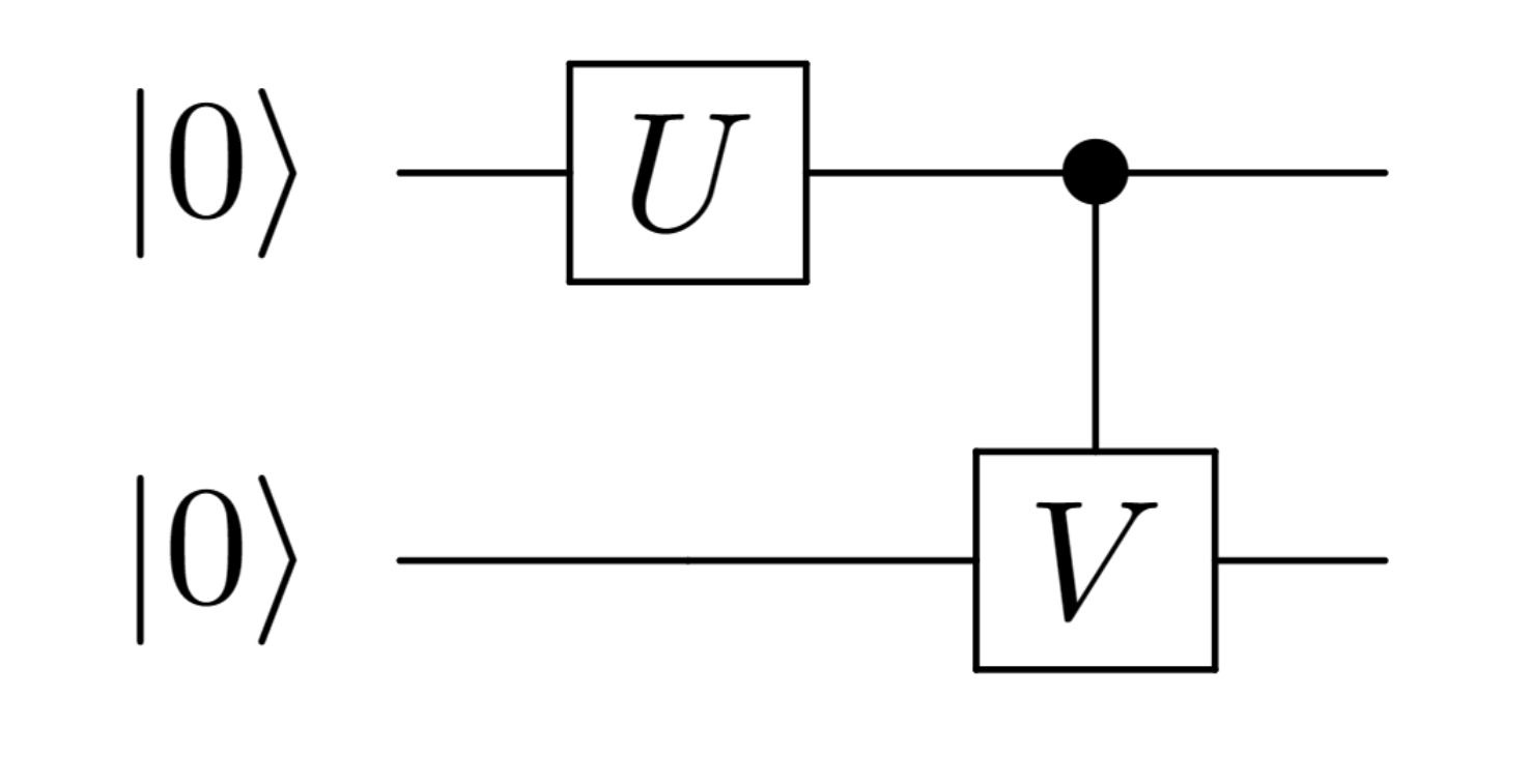
This circuit returns the realization of as a 2-qubit state:
| (43) |
In this way, we rule out all trivial contribution to the non-stabilizerness, isolating only the significant ones.
For the particular case of we can prove that the magic produced by the operators and is 0; i.e. is a stabilizer state. Let us write the matrix form of the operators:
| (44) |
| (45) |
We consider the state , which in the Pauli basis reads
| (46) |
The magic of the basis state is
| (47) |
Since the trace of the product of Pauli matrices is equal to only if the product returns and otherwise, among the terms of the sum in (47) there are only four non vanishing contributions, which are the ones with equal to one of the terms in the Pauli decomposition of the state. Equation (47) returns
| (48) |
Namely, the intertwiner state is a stabilizer state.
We now repeat the same procedure for the state . First, we realize the operators as matrix:
| (49) |
| (50) |
The action of this operators on returns
| (51) |
We write the state as
| (52) |
There are ten non-vanishing contributions to the magic of this state, each of which is equal to the fourth power of one of the coefficients of (52). Direct calculation returns
| (53) |
Appendix B Average SE gap
In this section, we show the details of the calculations of the average SE gap shown in Section V,
| (54) |
with denoting the unitary group average with respect to the Haar measure, being the linear SE, being the dimensions of the Hilbert spaces involved (recall that is the dimension of the gauge invariant intertwiner space, hence , whereas is the dimension of the ambient -qubit space, thus ), and
| (55) |
with being the Pauli group on qubits modulo the phases.
B.1 Haar averages and calculation of
We start by calculating since it is the simplest one: plugging the definition of in the Haar average reads
| (56) |
since the Haar average is linear. Our focus, then, is on evaluating
| (57) |
In general, carrying out the Haar average of operators of the form requires the knowledge of the commutant of the -tensored representation of the unitary group, according to Schur’s Lemma. By the Schur-Weyl duality, the basis of the full commutant of is constituted by the permutation operators acting over the copies of the Hilbert space of interest. In particular, the average of the copies of a state is carried out in detail in [66], and reads
| (58) |
with
| (59) |
being the projector onto the subspace of which is symmetric under permutations of objects. The result of this average is to be expected by the fact that operators belonging of the form are actually symmetric under permutation operators, so the weight associated to each of this operators must be the same and is hence only determined by the normalization.
The permutation operators relative to can be written in the computational basis of , namely in this way:
| (60) |
Notice that the permutation operators are invariant under -copies of unitary operators : this means that such operators will have the same expression in any basis of . Now, starting In our case, we are interested in the Haar average of four copies of the state, namely
| (61) |
Substituting this expression in Eq. (57) we get
| (62) |
In order to tackle this calculation, one calculates the sums of the Pauli operators permutation by permutation: by means of example, we show the calculation for one permutation, but the treatment is similar for all of them. Let’s take, say, the -cycle : the permutation operator associated to this permutation reads
| (63) |
hence
| (64) |
where we used the fact that and . Executing similar calculations for the other elements of and summing all the contributions, one gets
| (65) |
hence
| (66) |
B.2 Haar Averages on subspaces: proof of Lemma 1
Let generic Hilbert space decomposed in two orthogonal subspaces, with , and , and the projector onto being
| (67) |
Applying the formula shown in Eq. (61), the average onto the subspace reads
| (68) |
whereas if we calculate the average onto the full Hilbert space we get
| (69) |
Now, it suffices to check that the action of copies of the projector onto the permutation operators representation on the full Hilbert space gives the permutation operators representation on the subspace . Applying the expression shown in Eq. (60) for the permutation operators to this case we get
| (70) |
One then notices that
| (71) |
hence Eq. (70) reduces to
| (72) |
Using this result, Eq. (68) reads
| (73) |
which completes the proof.∎
B.3 Calculation of
In this subsection, we use the result of Eq. (73) to calculate , which reads
| (74) |
and in particular, we focus on the evaluation of
| (75) |
| (76) |
with . We can plug the generic formula shown in Eq. (61) and getting
| (77) |
The relevant difference between this calculation and that carried out in Eq. (66) is the representation of the permutation operators : they now read
| (78) |
with all indices belonging to as written in Eq. (11). These are indeed operators acting on , but they are not the full permutation operators of , since the indices of the sums do not run on all the basis elements of , but only on the intertwiner basis elements. Substituting this expression (and the one in Eq. (73)) in Eq. (75) we get
| (79) |
The previous observation renders the calculation of objects like slightly more difficult, since we cannot exploit the completeness relationship of basis elements like we did in Eq. (64), simply because is not a complete basis for . However, by pure brute-force methods, we are able to evaluate this object. We proceed permutation by permutation, as before: the trace of with a single permutation operator reads
| (80) |
This sum is constituted by products of matrix elements of matrices between two intertwiner basis elements, which are -component vectors in the original basis. By separately calculating the four possible matrix elements for each and every of the operators of (namely, ), and combining them according to the permutation , and them summing over the Pauli operators , one is able to compute objects of the form (80). Repeating this method for the permutation operators of and summing the results one gets
| (81) |
hence
| (82) |
and finally, we can evaluate the average SE gap, which reads
| (83) |
Appendix C SE of 4-valent intertwiner with generic spin
In this section, we introduce a generalized version of the Stabilizer Entropy for qudit systems, following the lines of [48]. This generalization is needed since the dimension of the intertwiner Hilbert space associated with a quantum tetrahedron with all spins equal to is , according to Peter-Weyl’s theorem. Indeed, we can write explicitly the intertwiner state in (8) as
| (84) | |||||
where the states form a set of mutually orthogonal basis elements in the singlet subspace of the Peter-Weyl decomposition of the original Hilbert space. Hence, the projector on the gauge invariant subspace is
| (85) | |||||
For , this implies that the intertwiner Hilbert space is not a -level system; thus, the usual formulation of stabilizer entropy for qubit systems cannot be applied to such a case.
In order to establish a definition of Stabilizer entropy for generic qudit systems, we introduce the generalization of Pauli group, namely the discrete Heisenberg-Weyl group. Consider an -dimensional Hilbert space and the space of linear operators acting on it, namely : we define the boost and shift operators as
| (86) | ||||
| (87) |
with . The Heisenberg-Weyl operators are defined as
| (88) |
with . They form a basis for , given by the operators , where the orthogonality relation reads
| (89) |
Finally, the Heisenberg-Weyl group is defined as the group generated by such operators:
| (90) |
Notice that for the Heisenberg-Weyl group reduces to the usual Pauli group for qubit systems.
The Heisenberg-Weyl group acting on a qudit system is simply given by the tensor product of copies of the Heisenberg-Weyl group for one qudit.
| (91) |
Any qudit state can be written in the Heisenberg-Weyl basis as follows
| (92) |
with . We can define the normalized expected value of a qudit pure state over the discrete Heisenberg–Weyl operators as and the -Stabilizer Rényi Entropy on qudit systems reads
| (93) |
In order to compute the SE of a quantum tetrahedron state with , we can refer to (8) and write the intertwiner density matrix and its tomography in the Heisenberg-Weyl basis
| (94) | ||||
| (95) |
where the sums over and run from to and the ones over and run respectively from to and from to ; is the dimension of the Hilbert space over which the trace is performed.