IR-Aware ECO Timing Optimization Using
Reinforcement Learning

Abstract.

Engineering change orders (ECOs) in late stages make minimal design fixes to recover from timing shifts due to excessive IR drops. This paper integrates IR-drop-aware timing analysis and ECO timing optimization using reinforcement learning (RL). The method operates after physical design and power grid synthesis, and rectifies IR-drop-induced timing degradation through gate sizing. It incorporates the Lagrangian relaxation (LR) technique into a novel RL framework, which trains a relational graph convolutional network (R-GCN) agent to sequentially size gates to fix timing violations. The R-GCN agent outperforms a classical LR-only algorithm: in an open 45nm technology, it (a) moves the Pareto front of the delay-area tradeoff curve to the left and (b) saves runtime over the classical method by running fast inference using trained models at iso-quality. The RL model is transferable across timing specifications, and transferable to unseen designs with zero-shot learning or fine tuning.

1. Introduction

Power integrity in ICs involves meticulous tools and flows for power grid analysis and optimization (OpeNPDN, ) that restrict the IR drop in the grid below a specified limit, and timing optimization uses gate delay models at this worst-case voltage corner. Due to limited wiring resources, in late stages of design, the power grid may not meet the IR limit, resulting in increased gate delays and timing failures. By then, the power grid has been designed and the placed and routed layout is near-final, so large perturbations will impede timing closure; only incremental engineering change order (ECO) optimizations, with minimal placement perturbation, are allowable to resolve timing violations. We address the ECO timing optimization problem to resolve late-stage violations through gate sizing.

Gate sizing for early design stages has been well studied, but there is little work on ECO for IR-induced timing failures. Gate sizing selects a size for every netlist instance from a set of choices in the standard cell library, each with different delay/area/power, and is NP-hard (tilos, ). Early approaches used simple convex models in a space of continuous gate sizes, using sensitivity methods (sensitivity-abk, ), convex programming (convex, ), and Lagrangian relaxation (LR) (chu2, ). The modern version uses more complex nonconvex delay models and discrete gate sizes (chu1, ). ECO-based optimizations in (Chang13, ; Lee14, ) do not address the interaction between IR drop and gate sizing. In (Lin20, ), ECOs for IR drop are resolved by moving cells; results show large placement perturbations. Our ECO solution performs low-perturbation sizing to meet timing and is based on reinforcement learning (RL).

RL has been applied to several chip design problems (google-rl, ; gcn-rl, ; survey-rl, ). Prior methods have tackled the related gate sizing problem at early stages of design, without supply voltage awareness (rl-sizer, ; lr-gnn-sizer, ). In (rl-sizer, ), RL is applied in a black-box framework, trained from scratch with very little problem-specific knowledge; in (lr-gnn-sizer, ), imitation learning is used rather than RL, merely accelerating LR methods to explore delay-area Pareto tradeoffs rather than fully harnessing RL.

Prior RL methods for gate sizing cannot be trivially extended to the ECO problem, but it is useful to examine their limitations. First, they incur forbidding runtimes due to the large action and search spaces for optimization. Second, they focus on a single objective (e.g., minimizing TNS in (rl-sizer, )), rather than the full multi-objective constrained optimization problem. Using penalty- and weight-based techniques that combine power, area, and timing into a single loss function requires significant parameter tuning per design (mo-rl, ) and is not viable. Third, they use RL as a “black box” optimizer rather than weaving in prior advances in gate sizing to build a solution that combines the best of traditional and ML-based solvers.

We overcome the first issue through the very nature of our ECO problem formulation: the requirement for minimal perturbation to the existing solution naturally results in action and search spaces of manageable size. To address the second and third issues, we eschew the black-box approach, and instead, leverage domain- and problem-specific knowledge, using LR to drive RL by coupling novel RL techniques with essential ideas from prior LR-based approaches. The use of Lagrange multipliers (LMs) from LR also provides a natural way to solve constrained optimization problems. The use of problem-specific insights also addresses the first issue by improving the efficiency of RL, which is well known to be sample-inefficient (rlblogpost, ).

We propose RL-LR-Sizer, leveraging advances in deep RL coupled with traditional LR-based techniques to solve the constrained optimization problem of ECO gate sizing. The sizing problem iteratively answers one of the following questions in each RL iteration: (i) Order: “Given a circuit netlist, which gate to operate on (upsize or downsize)?”, and (ii) Choice: “Given a gate and its local neighborhood, what size to select?” RL-LR-Sizer uses a relational graph convolutional neural network (R-GCN) as an agent to solve the order and choice problems. The agent is trained using deep Q learning (dqn, ), interacting with the environment to maximize a reward. The reward function is defined by converting the constrained optimization problem into an unconstrained problem using LMs, which are updated during the training iterations. Our key contributions are:
(1) This is the first work to address ECO sizing for library-based NLDM delay models under an RL-based framework.
(2) We couple RL with LR-based techniques to train an R-GCN agent to determine both order and choice. This naturally enables multi-objective optimization, presenting the first RL formulation for constrained gate sizing. We also leverage problem-specific knowledge in gate sizing to help RL find better solutions.
(3) Our novel clock update method (Sec. 4) during training enhances model quality over a range of timing specifications.
(4) We train the RL-LR sizer and use it for inference for multiple ECO changes, and at multiple timing specifications, and across multiple designs. We show (a) a full training flow per design; (b) zero-shot inference flow using a trained model on an unseen timing specification on a seen or unseen design; and (c) fine tuning flow on a trained model.

2. Problem formulation

The ECO problem is encountered late in the design cycle, after place-and-route and power grid design. Larger-than-expected IR drops result in increased gate delays, and the circuit fails timing. The ECO step resizes devices to bring the circuit back to timing specifications. This involves both device upsizing (to improve drive strength) and downsizing (to reduce the load offered to the previous stage). In principle, upsizing/downsizing could change the current load and alter the voltage drop, but empirically, the change in current load is small, resulting in supply voltage changes (0.001% of a 1.1V supply).

Formally, the objective of IR-aware ECO timing is to minimize the total area (or leakage power) of the design while satisfying performance and electrical constraints after considering post-PD IR drop. The constrained optimization problem is formulated as:

(1) $$\operatorname*{minimize}\; \;\textstyle\sum_{i\in\mathcal{I}}Area_{c_{i}}\;\;$$

subject to $$\;-\mathrm{slack}_{i}(V_{dd,i},GND_{i})\leq 0\;\;\forall i\in\mathcal{I}$$

$$\;c_{i}\in\mathcal{C}_{i}\;\;\forall i\in\mathcal{I}$$

where $\mathcal{I}$ is a set of instances; $\mathcal{C}_{i}$ is the set of choices for instance $i$ in the library; $c_{i}\in\mathcal{C}_{i}$ is the library cell assigned to instance $i$; $\mathrm{Area}_{c_{i}}$ is the area of instance $i$; and slack_i is the slack at instance $i$ as a function of post-PD rail voltages, $V_{dd,i}$ and $GND_{i}$. The constraint on slack_i uses “$\leq$” form for nonnegative Lagrangian multipliers.

The primal problem (1) is translated (BV09, ) to an unconstrained problem using a nonnegative Lagrange multiplier (LM), $\lambda_{i}$, for each slack constraint, yielding the Lagrangian objective function:

(2) $$\boldsymbol{L_{\lambda}}(c,\mathrm{slack}):\textstyle\sum_{i\in\mathcal{I}}Area_{c_{i}}\\ +\sum_{i\in\mathcal{I}}L_{slack,i}$$

(3) $$\mbox{where }L_{\text{slack},i}=\begin{cases}\frac{\lambda_{i}(-\mathrm{slack}_{i})}{\beta\times\mathrm{TNS}+\epsilon_{0}}&\text{if $\mathrm{TNS}\leq\alpha\times\mathrm{clk}$ }\\ \lambda_{i}(-\mathrm{slack}_{i})&\text{otherwise}\\ \end{cases}$$

and $\boldsymbol{\lambda}$ is the vector of $\lambda_{i}$s. Here, $\alpha$ and $\beta$ are tunable constants and $\beta<0$, $\epsilon_{0}$ is a small value to prevent divide-by-zero; $\mathrm{clk}$ is the clock period; TNS is the sum of the negative slacks over all instances; and $c$ [$\mathrm{slack}$] is a set variable for $c_{i}$ [$\mathrm{slack}_{i}$]. We use $L_{\text{slack},i}$ to provide a higher importance to the slack component of the Langrangian as the slacks approach zero. This idea leads to the LR subproblem (LRS) formulation for gate sizing (chu1, ), which, for a given $\boldsymbol{\lambda}$ is:

(4) $$\begin{aligned} \mbox{\bf LRS: }&\textstyle\operatorname*{minimize}_{c,\mathrm{slack}}&L_{\lambda}(c,\mathrm{slack})\\ &\text{subject to}&c_{i}\in\mathcal{C}_{i}\;\;\forall i\in\mathcal{I}\end{aligned}$$

LR solves the unconstrained problem (1), iteratively updating the LMs $\boldsymbol{\lambda}$, and hence (4), using a strategy described in Section 3.

We embed the above objective function into an RL framework as a reward and train an R-GCN agent to solve the LRS. Although we formulate the problem for area minimization, our approach can be applied to minimize power. The LRS solver, which minimizes the weighted sum of slack and the area, can trivially be modified for a power (leakage + dynamic power) objective function.

3. RL-LR ECO timing framework

The RL-LR ECO timing framework solves (4) by:
(a) Representing the netlist as a graph with node-level features;
(b) Mapping the sizing problem to an RL-solvable control problem;
(c) Developing a deep Q-network (DQN) framework, coupled with an LM update strategy, for training the R-GCN model (RL agent).

3.1. The circuit netlist as an annotated graph

The circuit netlist is represented as a directed relational graph $G=(\mathcal{V},\mathcal{E},\mathcal{R})$ where $\mathcal{V}$ is a set of all nodes representing the instance in the design, $\mathcal{E}$ is a set of all edges representing the nets in the design, and $\mathcal{R}$ is a set of all possible relation types that represent the input or output relation of each edge to the node in the graph. We convert the hyperedges in the circuit to a star representation (fastplace, ) where each wire from instance $i$ to instance $j$ is represented by a edge $(v_{i},r,v_{j})\in\mathcal{E}$ with relation $r$. The graph representation of the netlist allows us to solve the gate sizing problem through the use of deep RL algorithms.

The nodes in the graph are annotated by a list of features (Table 1), used by the R-GCN agent that are capable of understanding the relations between nodes to make decisions. In our work, R-GCNs understand edge directions as the gate delay is dependent on identifying the driver and loads. R-GCNs accumulate annotated features from the set of neighbors, $\mathcal{N}_{i}^{r}$, of instance $i$ under relation $r\in\mathcal{R}$. From outgoing edges and incoming edges, R-GCN aggregates different features from neighbors. The output load capacitance is only aggregated from outgoing edges, and the input slew is only aggregated from incoming edges. All other features are aggregated from both edges. The slack, slew, load and IR voltage drop features help the R-GCN agent make decisions that meet timing constraints. The instance type feature enables the agent’s decisions to minimize area and meet timing.

Table 1. List of the annotated features on instance $i$ in $G$.

Feature	Definition
$\mathrm{slack}_{i}$	Slack at the output pin.
$\mathrm{in\_slew}_{i}$	Maximum slew at the input pins.
$\mathrm{out\_slew}_{i}$	Slew at the output pin.
$\mathrm{instance\_type}$	Size and type of cell.
$\mathrm{load}_{i}$	Capacitive load at the output pin.
$\mathrm{ir\_voltage}_{i}$	Power supply voltage at th cell with IR drop considerd.

Figure 1. State and action spaces from the circuit netlist.

3.2. Mapping IR-aware gate sizing to RL

We map the sizing problem (4) to a Markov Decision Process (MDP), making sequential RL-based decisions. We define the following:

State: The state $s_{t}$ at step $t$ is a subgraph of the annotated graph $G$ that contains all instances $v_{i}$ that have $\mathrm{slack}_{i}<0$, or lie within a two-hop neighborhood of any instance with $\mathrm{slack}_{i}<0$. Unlike (rl-sizer, ), which uses a local embedding of a single independent instance and its three-hop neighborhood as the state, we use all netlist instances with negative slack and their neighborhood as the state, letting the RL agent decide which instances in the state to operate on.

Fig. 1 illustrates the state $s_{t}$ at time step $t$ (on this toy example, $s_{t}$ is a large fraction of the circuit, but for a large circuit [des_perf. 25k gates], $s_{t}$ contains only 0.06% of the gates). The red instances correspond to gates on the critical path (most negative slack) after considering IR drop impact, the yellow instances correspond to gates that also have negative slack (near-critical paths) and the purple gates are those that belong to the two-hop neighborhood of any instance with $\mathrm{slack}_{i}<0$ (red or yellow instances). This state representation provides the RL agent with a global view of the graph, preventing the optimizer from being stuck within local minima. In contrast, (rl-sizer, ; lr-gnn-sizer, ; chu1, ) operate with a single instance (the instance being sized in the current iteration), and its immediate neighborhood as the state. Mimicking these methods would provide an RL agent with little local information, leading to local minima.

Action: We define an action as both the order (which gate is selected) and choice (whether it is upsized or downsized). Instead of using all nodes in the state as the action space, we prune the space for faster convergence of RL training by creating an action mask:

(5) $$\phi(x_{a})=\begin{cases}x_{a}&\text{if $a$ is a valid action}\\ 0&\text{otherwise}\\ \end{cases}$$

The mask constrains the agent to select gates that are on, or within a two-hop neighborhood of, any gate on the critical path. The size of the action space, which is based on the critical path only, is a small fraction of the state space for large circuits. The mask also prevents invalid actions, e.g., upsizing a gate at its largest available size. In Fig. 1, all instances highlighted in dotted circles are within the action space. The action space size is twice the number of candidate gates, as each gate can be either upsized or downsized.

Based on the state and action spaces, we set up the gate sizing RL formulation. However, the action space is large, creating challenges for the already sample-inefficient RL algorithm (rlblogpost, ). We limit the size of the action space by coupling RL training with problem-specific knowledge from LR-based gate sizing, as described Section 4.2.

Reward: The reward $R_{t}$ is the consequence of the action $a_{t}$ on state $s_{t}$. For the ECO gate sizing problem in Section 2,

(6) $$R_{t}=L_{\lambda}^{t}(c,\text{slack})-L_{\lambda}^{t+1}(c,\text{slack})$$

where $L_{\lambda}^{t}(c,\text{slack})$ and $L_{\lambda}^{t+1}(c,\text{slack})$ is the value of the LRS-based objective function at steps $t$ and $t+1$, respectively, due to action $a_{t}$. Since $a_{t}$ changes the size of only one gate, with every action, we perform an incremental timing update to evaluate $L_{\lambda}^{t+1}(c,\text{slack})$.

RL agent (R-GCN): GCN-based agents that work on a graph create effective representations of the circuit that encode features into a meaningful embedding through a message passing scheme.

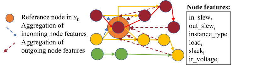
Figure 2. R-GCN node aggregation from a 3-hop neighborhood.

The aggregation for the ECO sizing problem is shown in Fig. 2, for the reference node highlighted in orange, corresponding to the state in Fig. 1. The propagation model for calculating the forward-pass update of a node, $v_{i}$, in the circuit graph is defined by the following computation performed in layer $l$ of the R-GCN:

(7) $$h_{i}{(l+1)}=\sigma\left(W_{o}(l)h_{i}(l)+\sum_{r\in\mathcal{R}}\sum_{j\in\mathcal{N}_{i}^{r}}\frac{1}{d_{i,r}}W_{r}(l)h_{j}(l)\right)$$

where $\mathcal{N}_{i}^{r}$ is the set of neighbors, and $d_{i,r}$ the normalizing constant, for instance $i$ that have the relation $r$. The relation $r$ is the edge direction in our R-GCN. In layer $l$, $h_{i}(l)$ is the hidden state of the node $v_{i}$; $W_{r}(l)$ is the weight matrix of the neural network layer $l$ for the relation $r$. The accumulated features are separately and linearly combined for each direction type with the weight matrix $W_{r}(l)$. The values are normalized by the degree of the node $i$ for the relation $r$, $d_{i,r}$. $W_{o}(l)$ is the weight matrix for self features; and $\sigma(.)$ is an activation function (we use $\mathrm{ReLU}$). This propagation model is applied to subgraph $s_{t}$ to generate $h_{i}(l+1)$ in layer $l+1$.

Fig. 3 shows the structure of the R-GCN agent, with three R-GCN layers, i.e., each node aggregates features from a three-hop neighborhood. The first two layers, each of dimension 64, are followed by ReLU activation functions. The last layer is fed to the action mask to generate a valid action that maximizes the reward.

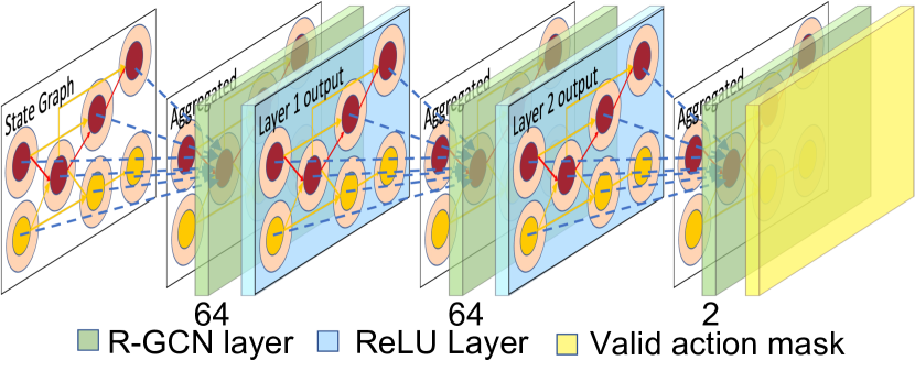
Figure 3. Structure of the three-layered R-GCN agent.

Environment (Env): The environment includes components that interact with the agent: in our case, this is the inbuilt timing engine that estimates the reward and updates the graph based on an action.

3.3. Application of the R-GCN agent

We apply our R-GCN agent on a post-PD netlist. Fig. 4 highlights the gate sizing flow and shows how the R-GCN agent interacts with the environment. We represent the netlist as a graph $G=(\mathcal{V},\mathcal{E},\mathcal{R})$ and extract the node-level features. Based on the annotated features, we create $s_{t}$, and the action mask $\phi$. The R-GCN agent acts on $s_{t}$ to perform action $a_{t}$. As a consequence of $a_{t}$, the environment performs incremental timing analysis, updates the circuit netlist, and computes $R_{t}$. A new state is created using the updated netlist and the new features, and the loop is repeated until TNS, WNS, or area converges. The resulting netlist is near-optimally sized and meets the delay constraints while minimizing the total area.

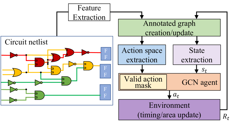
Figure 4. R-GCN sequentially sizes gates, maximizing reward.

4. RL model training

4.1. Core training strategy

We use a deep-Q network (DQN) training algorithm (dqn, ) coupled with an LM update strategy (chu1, ) to train the R-GCN. In the DQN framework, the R-GCN, known as the Q network ($Q(s,a;W)$), is an approximator for the best action-value function, $Q^{*}(s,a)$, to select actions that maximize expected cumulative reward, defined as:

(8) $$Q^{*}(s,a)=\mathbb{E}\left[R+\gamma\max_{a^{\prime}}Q^{*}(s^{\prime},a^{\prime}|s,a)\right]$$

This expression obeys the Bellman equation, which is based on the idea that if the optimal value $Q^{*}(s^{\prime},a^{\prime})$ in the next time step is known for all possible actions $a^{\prime}$ from state $s^{\prime}$, the optimal strategy selects action $a^{\prime}$ to maximize $\mathbb{E}[R+\gamma Q^{*}(s^{\prime},a^{\prime})]$, where $\mathbb{E}(.)$ is the expected value; future rewards are discounted by $\gamma$ per time step $t$.

DQN training: We leverage the DQN training framework described in (dqn, ) which begins by initializing a memory replay buffer of capacity $N$, and random initial R-GCN weights. The training iterates over $M$ episodes, with each episode containing $T$ timesteps. During each timestep, an action is taken based on an $\epsilon$-greedy policy strategy where it selects an action from the R-GCN with probability $(1-\epsilon)$ and selects a random action with probability $\epsilon$. Initially, the training begins with a high value for $\epsilon$, encouraging the agent to explore the environment, and decays every episode to a smaller value exploiting the knowledge the agent has gained. We apply the action mask and select an action from the available valid candidates.

Based on the chosen valid action, $a_{t}$, the environment updates the area and timing incrementally and computes $R_{t}$. The transition which includes $s_{t}$, $s_{t+1}$, $a_{t}$, and $R_{t}$ is stored in a replay buffer at each step. The buffer is sampled at every step to extract a batch of random samples that train the R-GCN policy network. To make training more stable, the DQN training uses a target network, which keeps a copy of R-GCN weights to estimate the $Q^{*}(s^{\prime},a^{\prime})$ value in the Bellman equation. The target network is updated every $C$ episodes by copying the weights from the policy network. The R-GCN policy agent is trained by minimizing the loss function:

(9) $$Loss(W)=\mathbb{E}_{s,a,R}\left[(\mathbb{E}_{s^{\prime}}[y|s,a]-Q(s,a;W))^{2}\right]$$

where $y=\mathbb{E}_{s^{\prime}}[R+\gamma\max_{a^{\prime}}\hat{Q}(s^{\prime},a^{\prime},\hat{W})|s,a]$ uses the target network $\hat{Q}(s^{\prime},a^{\prime},\hat{W})$ to estimate the discounted future rewards. The target network weights $\hat{W}$ are fixed when optimizing the loss function.

Env reset: We use a modified environment reset strategy in comparison to (dqn, ). At the beginning of each episode, instead of resetting the graph to its original state at the beginning of the first episode, we reset the graph to the state which has the least $\mathbf{L_{\lambda}}(c,slack)$ in the previous episode. This allows for faster convergence of the objective function during training iterations due to guided explorations.

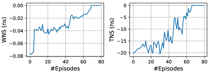
Figure 5. Converging WNS and TNS during training.

4.2. Problem-specific training enhancement

We incorporate gate-sizing-specific optimizations into the general training framework to enhance the quality of the trained model.

Clock constraint update. To make the model transferable across different start points within a design, the clock is updated every episode. We start early episodes of training with a negative slack to more gently nudge RL towards the required clock period and encourages reduced delays; in the absence of this strategy, most RL episodes fail as the chances of meeting the period is small.

In the first $M_{decay}$ of $M$ total episodes, the clock constraint decays linearly: at the start of each episode, the clock constraint is reduced by $\frac{(\text{initial\_delay}-\text{target\_delay})}{\mathrm{M}_{decay}}$, where initial_delay is the delay in post-placement and post-PDN synthesis with IR-drop impact considered and target_delay is the required delay. After $\mathrm{M}_{decay}$ episodes, the clock constraint reduces to target_delay, and is kept unchanged in the remaining training episodes. We set $\mathrm{M}_{decay}=30$.

To facilitate transferability across multiple designs and start points, we encapsulate away design-specific information and clock information into the state variable. We work with the lambda slack sum, i.e. $\sum_{i\in\mathcal{I}}L_{slack,i}$ in eq. (2), as the loss function, where the slacks are normalized by clock value set in each episode, instead of absolute delay values, which may vary from circuit to circuit.

Lagrangian multiplier (LM) update. The use of LMs to determine the relative weights of the components of the cost function is a crucial problem-specific insight used in this work. A direct application of RL would use fixed user-defined weights for $\lambda_{i}$, but instead, we use LR-based update strategies to drive RL exploration. Specifically, we embed the following LM update strategy during DQN training, where we update the values of $\lambda_{i}$ every $K$ steps within an episode: $\lambda_{i}=\lambda_{i}\times\left(1-\frac{slack_{i}}{clock\,period}\right)$. The strategy penalizes large violations more severely than smaller violations. This update strategy helps with guided explorations within the action space. When $\mathrm{slack}_{i}$ is positive or equal to zero, we set the corresponding $\lambda_{i}$ to zero.

ECO-based action space reduction. The ECO problem naturally reduces the sizes of the state and action spaces: given a generally good power grid, it is likely that only some combinational blocks of the sequential circuit, in IR-affected regions will require ECOs. Only gates in these regions will be part of the RL formulation.

Sensitivity-based action space reduction. A mask based on the sensitivity of the total delay change of a local graph to the size change of the center node is applied to reduce action space. The top 5–10% actions that most degrade the delay are pruned.

Fig. 5 shows the effectiveness of these approaches in training for circuit wb_conmax. At the end of $M$ episodes, we see that TNS and WNS have converged. Once trained, the R-GCN agent (target network) is applied to the circuit netlist (see Section 3.3) to sequentially select actions that solve the constrained optimization problem.

5. RL-LR ECO Timing Evaluation

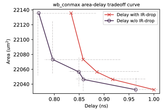
Figure 6. Delay-area tradeoff curves for wb_conmax in a 45nm technology, showing a shift to the right due to IR drop.

Table 2. ECO timing result comparison for three different flows in area, runtime, cell change metrics

Designs	Target Delay (ns)	Initial Delay (ns)	Area($\mu$m2)					Runtime(s)				# of Upsize/Downsize
			LR	Inference across Timing Constraints		RL-LR Training		LR	Inference across Timing Constraints		RL-LR Training	LR	Inference across Timing Constraints	RL-LR Training
des_area	0.56	0.5896	2436.3	2460.5	-0.99%	2424.6	1.24%	113	33	70.80%	2251	48/1	74/2	26/4
wb_dma	0.47	0.4859	4748.1	4751.3	-0.07%	4740.4	0.16%	29	14	51.72%	2285	12/0	9/0	8/3
pid_controller	0.75	0.7814	5520.3	5513.9	0.12%	5499.3	0.38%	107	26	75.76%	2718	29/2	25/4	26/6
aes_cipher_top	0.89	0.9412	14799.0	14486.0	2.12%	14460.0	2.29%	127	113	55.52%	3015	386/3	99/0	103/1
des_perf	0.60	0.6318	27454.0	27274.0	0.66%	27183.0	1.19%	354	103	70.79%	3103	347/1	230/0	185/1
pci_bridge32	0.75	0.7805	25828.0	25824.0	0.02%	25824.0	0.02%	78	51	34.19%	2794	24/1	21/1	24/3
wb_conmax	0.81	0.8581	22195.0	22130.0	0.29%	22108.0	0.39%	241	125	48.13%	3123	81/0	55/0	45/2
Average					0.30%		0.81%			58.13%
Maximum					2.12%		2.29%			75.76%

5.1. Experimental setup

We use Design Compiler to size a set of gate-level netlists under various timing constraints at the supply voltage corner; the design is then placed using Innovus, the power delivery network is synthesized, and the static IR drop is analyzed using OpenROAD (openroad, ). An example delay-area curve for wb_conmax is shown as “Delay w/o IR-drop” in Fig. 6. We simulate larger IR drops in the PDN by manually adjusting per-unit RC values in the metal layers to achieve low ($\sim$5mV) and moderate ($\sim$10mV) maximum IR drop across the designs; we do not consider high IR drops that would require major changes rather than ECOs. To quantify the impact of IR drop on delay, we annotate NLDM entries of each library cell with the delay sensitivity to voltage drop, and compute circuit delays using the OpenSTA timing engine. Due to limitations of the characterized NanGate45 library, we obtain these sensitivities from a similar library in another technology. Under IR drop, the delay-area curve shifts to the right, from the “Delay w/o IR-drop” to the “Delay with IR-drop” curve in Fig. 6: for the same sized netlist, the area remains the same but the delay degrades due to IR drop.

The RL-LR ECO timing (training and application) flow is built using Python libraries, including PyTorch and DGL (karypis20, ). We create Python enablements for incremental timing analysis, logic gate swap, and pin and cell property from OpenROAD APIs using SWIG, which integrates easily into Env for reward computation and state transitions. OpenROAD eliminates challenges related to slow interfaces between TCL-dependent commercial tools and Python environments mentioned in (rl-sizer, ). We train the R-GCN agent using the hyperparameters $M=50$; $N=4000$; $T=75$; $\gamma=0.99$; $\alpha=10$; $\beta=-0.1$; $C=25$; $K=30$. These parameters are chosen by manual tuning for RL training convergence (Fig. 5).

Our experiments are performed on 7 OpenCores benchmarks using an open 45nm technology. We implement multiple flows:
(1) RL-LR ECO Training (Table 2) trains an R-GCN model from scratch for ECO, starting the initial delay and continuing until the target delay is achieved.
(2) RL-LR ECO Inference trains a model across a wide range of timing constraints to obtain the full delay-area Pareto curve. This training step is applicable for larger delay reductions than ECO optimizations, but requires more computation than that for ECO training. Given this trained model, we report:
(a) Inference across Timing Constraints (Tables 2 and 3) demonstrates transferability across timing specifications, running inference for different timing constraints on the delay-area trade-off curve of a design, using a model trained on the same design.
(b) Inference across Designs (Table 4) demonstrates transferability across designs, running inference for multiple designs using the model trained with four selected designs.
(c) Fine tuning (Table 4) further tunes the “Inference across Designs” model for a specific design. applying inexpensive fine tuning on the design to enhance the model.
(3) LR baseline (Tables 2, 3, and 4) implements a conventional LR-based flow (chu1, ) that the RL methods are compared against.

All runtimes are reported on a machine with Intel Xeon Silver 4214 CPU @2.2GHz and NVIDIA A100 PCIe 40GB GPU.

5.2. Optimization and delay-area tradeoffs

Table 2 compares the traditional LR baseline, RL-LR ECO Training, and Inference across Timing Constraints for the seven benchmark designs under the moderate IR drop scenario, for a specified target delay. The inference model is trained just once and has a training time of 4000-6000s, depending on the circuit. This is not much more than the runtime of RL-LR ECO training (reported in the table), because it requires 50 episodes for training, while RL-LR ECO training requires 30-40 episodes. Moreover, this training cost can be amortized over use for multiple ECO explorations during late-stage design, e.g., perturbations to routing, power grid design, or placement, each translating to altered slack, and thus covered by our formulation.

The table shows the initial delay of the circuit, i.e., the delay under the ideal IR drop; the area and runtimes for the three approaches; and the number of cell changes using the LR and RL-LR ECO training methods. It can be seen that the areas reported for the RL-LR ECO training outperform the LR-based flow, with 0.81% average and 2.29% maximum area improvement. Although the improvement numbers seem small, they correspond to area reductions in congested regions. The inference approach performs slightly worse than RL-LR ECO training, but provides solutions of similar quality, with some improvements.

The last columns of the table report the number of upsized and downsized cells: downsized cells can stay in place and do not require further changes to layout, but upsized cells require placement perturbations to remove overlaps. It can be seen that both Inference and RL-LR ECO training upsize a smaller number of cells compared to the LR-based flow, thus easing timing closure.

As is typical of RL-based approaches (rl-sizer, ; google-rl, ), RL-LR ECO training has very high runtime as it includes R-GCN training and a reward computation (STA update) during each of the $T$ steps of the training. The Inference across Timing Constraints model, with offline training, shows an average of 58.13% reduction over LR. After one-time offline training, the trained model can be applied to any operating period on the delay-area curve.

Table 3. Results of mutiple start points for wb_conmax design

Designs	Target Delay (ns)	Initial Delay (ns)	Area($\mu$m2)
			LR	Inference across Timing Constraints		RL-LR ECO Training
wb_conmax	0.77	0.8337	22297	22249	0.22%	22235	0.28%
	0.81	0.8581	22195	22130	0.29%	22108	0.39%
	0.85	0.8855	22097	22076	0.10%	22067	0.14%
	0.86	0.9173	22132	22077	0.25%	22065	0.30%
	0.96	1.0002	22046	22066	-0.09%	22037	0.04%
Average					0.15%		0.23%
Maximum					0.29%		0.39%

To demonstrate the model is transferable across multiple start points within a design, Table 3 presents results for five start points within a representative design, wb_conmax. The quality of result for the Inference flow is seen to be similar to the LR-based flow, and only slightly degraded over RL-LR training from scratch.

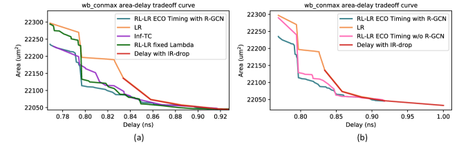
Figure 7. Delay-area tradeoff curves for wb_conmax highlighting the importance of LR to the RL-LR ECO timing.

5.3. Importance of LR and R-GCN in RL-LR ECO

In this section, we highlight the importance of three crucial aspects of the RL-LR ECO optimizer: (i) guided explorations through LR (ii) solving both the gate order and choice (gate size selection) problems (defined in Section 1) and (iii) the choice of R-GCN agent.

For circuit wb_conmax, Fig. 7(a) and (b) show the delay-area tradeoff curves for several flows: our trained RL ECO approach, the classical LR baseline, RL ECO Inference across Timing Constraints (Inf-TC), RL-LR with fixed lambda and RL ECO Training without R-GCN. Also shown is the red corner-based tradeoff curve, amended for IR-drop-induced delay degradation: this is identical to the “Delay with IR drop” curve in Fig. 6.

The yellow LR curve shows the classical solution. This curve coincides with the red curve up to a point, but can achieve lower delays. From Fig. 7(a), we see that the blue curve, corresponding to the RL-LR ECO optimizer, outperforms LR, generating a Pareto-optimal front that lies to the left of the delay-area tradeoff curves for LR. The purple curve, generated by Inference across Timing Constraints, also performs significantly better than LR, demonstrating transferability of the RL-LR ECO model across clock periods.

To understand the importance of using LMs to determine the relative weights of the objective function components, dynamically changed during the RL optimization, we consider the use of fixed $\lambda_{i}$ penalties for the slack term in (4) throughout the optimization, shown by the green curve. The use of fixed user-defined $\lambda$ values as weights is suboptimal as it predetermines and fixes the effort the optimizer makes towards meeting each conflicting term in the objective function. The blue RL-LR ECO timing curve and the purple Inference curve (based on a trained model) both use an R-GCN agent that updates $\lambda_{i}$ values, and both outperform the green fixed-$\lambda$ curve. The success of our RL-LR methods is ascribed to our RL-inspired methods that naturally enable the solution of constrained optimization problems, and eliminate the need for manual tuning of user-defined weights, and are formulated to solves the order and choice problems through RL.

To demonstrate the effectiveness of R-GCN, we replace the R-GCN with a traditional GCN, which averages features from all nodes together irrespective of the direction of the edge. Compared to the pink trade-off curve in Fig. 7(b) for a flow with traditional GCN, the blue curve for a flow with R-GCN that can differentiate between incoming and outgoing edges and shows the better quality of the generated solutions.

Table 4. RL transferability across designs

IR Drop	Designs	Target Delay (ns)	Initial Delay (ns)	Area($\mu$m2)					Runtime(s)
				LR	Inference across Designs		Fine Tuning		LR	Inference across Designs Or Fine Tuning (if needed)
Low ($\leq$5mV)	des_area	0.56	0.5676	2411.6	2409.2	0.14%	NA	NA	57	14	75.40%
	wb_dma	0.47	0.4859	4742.2	4741.2	0.02%	NA	NA	10	13	-26.80%
	pid_controller	0.75	0.7641	5508.9	5498.5	0.19%	NA	NA	112	15	86.29%
	aes_cipher_top	0.89	0.9083	14502.0	14428.0	0.57%	NA	NA	79	50	36.46%
	des_perf	0.59	0.6087	27125.0	27039.0	0.32%	NA	NA	319	144	54.86%
	pci_bridge32	0.75	0.7718	25827.0	25826.0	0.00%	NA	NA	78	11	85.46%
	wb_conmax	0.81	0.8286	22107.0	22074.0	0.15%	NA	NA	239	13	94.69%
Moderate ($\leq$10mV)	des_area	0.56	0.5896	2436.3	2426.5	0.40%	NA	NA	113	37	67.43%
	wb_dma	0.47	0.4859	4748.1	4759.8	-0.25%	NA	NA	29	23	19.31%
	pid_controller	0.75	0.7814	5520.3	5500.3	0.36%	NA	NA	107	19	81.93%
	aes_cipher_top	0.89	0.9412	14799.0	14479.0	2.16%	NA	NA	255	129	49.21%
	des_perf	0.60	0.6318	27454.0	–	–	27174.0	1.02%	354	458	-29.38%
	pci_bridge32	0.75	0.7805	25828.0	25827.0	0.00%	NA	NA	78	13	83.64%
	wb_conmax	0.81	0.8581	22195.0	–	–	22145.0	0.23%	241	493	-104.56%
Average						0.34%		0.37%
Maximum						2.16%		1.02%

5.4. Transferability across designs

To train a transferable model across multiple designs, we select four designs highlighted in blue in Table 4 and perform offline RL training. The table shows that in eight testcases, zero-shot inference (Inference across Designs) using the trained model can achieve the target delay; “–” represents an unachievable target delay. The model works for almost all testcases under low ($\leq$5mV) IR drop, but fewer in the moderate ($\leq$10mV) IR drop regime, as the timing degradation for the former is smaller and easier to fix.

In fact, since training across designs builds a “common” model for the four designs, the zero-shot model may fail to meet the target delay for an individual design out of the four. For other unseen testcases (circuits that are not blue) too, the target delay is often not met. For the testcases that do not admit a zero-shot solution, we further tune the trained model individually for each testcase through inexpensive fine tuning. We then achieve the target timing in all cases, and almost always have smaller area cost compared to the LR-based flow and with much smaller runtime than training from scratch. Note that designs that successfully met their target periods do not need fine tuning, as shown by “NA” (not applicable). Our runtime improvements are up to 64.35% over LR. In 10 of 14 testcases, our runtime is better than or equal to that for LR (one testcase is tied). For des_perf/Moderate IR drop, fine tuning shows area and runtime improvements.

6. Conclusion

We develop RL-LR ECO timing method to solve the constrained optimization problem of minimizing circuit area while fixing the timing degradation caused by IR drop. To enhance the ability of RL to find optimal solutions, we incorporate problem-specific knowledge into RL-driven gate sizing. Moreover, we propose a novel clock update method during training, which has demonstrated its effectiveness in enhancing model quality across multiple timing specifications and pushed the Pareto optimal front of the delay-area tradeoff curve to the left. Furthermore, the comprehensive analysis from a full training flow per design to zero-shot inference on unseen specifications, as well as a fine tuning flow on a pre-trained model, demonstrates the transferability and flexibility of our approach.

References

- (1) V. A. Chhabria et al., “Template-based PDN synthesis in floorplan and placement using classifier and CNN techniques,” in Proc. ASP-DAC, pp. 44–49, 2020.
- (2) J. P. Fishburn and A. E. Dunlop, “TILOS: A Posynomial Programming Approach to Transistor Sizing,” in Proc. ICCAD, pp. 326–328, 1985.
- (3) J. Hu, et al., “Sensitivity-Guided Metaheuristics for Accurate Discrete Gate Sizing,” in Proc. ICCAD, pp. 233–239, 2012.
- (4) K. Kasamsetty, et al., “A New Class of Convex Functions for Delay Modeling and its Application to the Transistor Sizing Problem,” IEEE T. Comput. Aid. D., vol. 19, no. 7, pp. 779–788, 2000.
- (5) C.-P. Chen, et al., “Fast and Exact Simultaneous Gate and Wire Sizing by Lagrangian Relaxation,” IEEE T. Comput. Aid D., vol. 18, no. 7, pp. 1014–1025, 1999.
- (6) A. Sharma et al., “Fast Lagrangian Relaxation-Based Multithreaded Gate Sizing Using Simple Timing Calibrations,” IEEE T. Comput. Aid D., vol. 39, no. 7, pp. 1456–1469, 2020.
- (7) H.-Y. Chang, et al., “ECO Optimization Using Metal-Configurable Gate-Array Spare Cells,” IEEE T. Comput. Aid. D., vol. 32, no. 11, pp. 1722–1733, 2013.
- (8) J. Lee and P. Gupta, “ECO Cost Measurement and Incremental Gate Sizing for Late Process Changes,” ACM T. Des. Automat. El., vol. 18, Jan. 2013.
- (9) H.-Y. Lin et al., “Automatic IR-Drop ECO Using Machine Learning,” in Proc. ITC-Asia, pp. 7–12, 2020.
- (10) A. Mirhoseini et al., “A Graph Placement Methodology for Fast Chip Design,” Nature, vol. 594, pp. 207–212, 06 2021.
- (11) H. Wang et al., “GCN-RL Circuit Designer: Transferable Transistor Sizing with Graph Neural Networks and Reinforcement Learning,” in Proc. DAC, 2020.
- (12) H. Ren et al., “Optimizing VLSI Implementation with Reinforcement Learning,” in Proc. ICCAD, 2021.
- (13) Y.-C. Lu et al., “RL-Sizer: VLSI Gate Sizing for Timing Optimization using Deep Reinforcement Learning,” in Proc. DAC, pp. 733–738, 2021.
- (14) X. Zhou et al., “Heterogeneous Graph Neural Network-based Imitation Learning for Gate Sizing Acceleration,” in Proc. ICCAD, 2022.
- (15) S. Huang et al., “A Constrained Multi-Objective Reinforcement Learning Framework,” in Proc. Conf. on Robot Learning, pp. 883–893, 2022.
- (16) A. Irpan, “Deep Reinforcement Learning Doesn’t Work Yet.” https://www.alexirpan.com/2018/02/14/rl-hard.html, 2018.
- (17) V. Mnih et al., “Playing Atari With Deep Reinforcement Learning,” in Proc. NeurIPS, 2013.
- (18) S. Boyd and L. Vandenberghe, Convex Optimization. Cambridge, UK: Cambridge University Press, 2009.
- (19) N. Viswanathan and C. C.-N. Chu, “FastPlace: Efficient Analytical Placement Using Cell Shifting, Iterative Local Refinement and a Hybrid Net Model,” in Proc. ISPD, p. 26–33, 2004.
- (20) “OpenROAD.” https://github.com/The-OpenROAD-Project/OpenROAD, 2022.
- (21) M. Wang et al., “Deep Graph Library: A Graph-Centric, Highly-Performant Package for Graph Neural Networks,” in arXiv:1909.01315, 2020.