On the effect of the luni-solar gravitational attraction on trees

Abstract

In this paper, we revisit old electrical measurements conducted on a poplar tree in 2003 (Gibert et al. 2006), which showed the presence of a diurnal electrical signal, attributed to an electrokinetic phenomenon correlated with sap flow, even in winter. We reanalyze these data using the singular spectrum analysis method and demonstrate that the electrical signal measured at various locations (roots, trunk, and branches) on the poplar tree can be decomposed to over 80% into a sum of 7 pseudo-periods, all linked to luni-solar tides. The precision of the extracted periods exceeds that of models. To validate these old measurements, we have reproduced the 2003 protocol since 2018 at the Jardin des Plantes in Paris, on 3 oak trees and 3 hornbeams. The electrical signals today exhibit the same characteristics as those of 2003. Tidal forces could be a driving force of sap flow in trees.

1 Introduction

Trees, like the majority of plants on our planet’s surface, can be broadly schematized as having a root system connected to branches through a trunk. Channels, such as phloem or xylem, originating from the rhizoderm and extending to the leaves, play a crucial role in facilitating proper irrigation and supplying nutrients for the plant’s growth. The fluid, varying in complexity based on its location within the plant, functions as its circulatory system and is commonly referred to as sap. A significant and ongoing debate revolves around the question of how this sap moves within the plant. In the literature, three main hypotheses are typically discussed to explain this movement. The first one involves capillarity (eg. [1, 2, 3, 4, 5]), the second revolves around osmotic pressure (eg. [6, 7, 8, 9, 10]) and the third, frequently debated hypothesis is that of evapotranspiration (eg. [11, 12, 13, 14]). This idea originates from climatologist Thornthwaite [15], who sought to identify various geophysical phenomena contributing to the transfer of liquid water from the Earth’s surface to the atmosphere, ultimately classifying different climates. Plant evapotranspiration is recognized as one of these phenomena, alongside snow sublimation and the evaporation of free water.

In their study of electrical signals measured on a standing poplar over the course of a year, Gibert et al. [16] demonstrated two important findings. Firstly, the recorded electrokinetic signals were associated with the sap flow in the tree (estimated by Ganier probes), and secondly, a diurnal oscillation, albeit modest, persisted even during the winter season.

For several decades in geophysics, it has been established and observed that changes in velocity in an established flow or the addition of a saline front lead to measurable variations in electrical potential. This electrokinetic phenomenon is commonly referred to as spontaneous potential (SP, eg. [17, 18, 19]).

In the natural environment, diurnal oscillations are not solely attributable to thermal fluctuations resulting from the alternation of day and night. Instead, they are generally linked to terrestrial gravitational tides caused by the combined influences of celestial bodies such as the Moon and the Sun (cf. [20]). Our planet experiences disruptions during its revolution and rotation, with the Moon and the Sun playing pivotal roles. These celestial interactions lead to phenomena like the precession of the equinoxes, which occurs over a period of approximately 26,000 years (for further details, see, eg. [21, 22]). In a broader context, mobile masses on the Earth’s surface oscillate under the influence of these luni-solar forces, with coastal tides being a primary manifestation. These forces also impact and vertically oscillate water confined in deep aquifers (eg. [23, 24, 25, 26, 27]), potentially influencing processes such as water-rock interactions (eg. [28, 29]). Consequently, these interactions may play a role in providing nutrients to plants (eg [30]).

We have demonstrated, over long periods exceeding 200 years, how the global series of volcanic eruptions activity (cf. [31]), the average sea levels evolution (cf. [32]) and the dynamics of the trees population within a Tibetan juniper forest (cf. [33]), could be decomposed into a series of cyclical patterns, all linked to the gravitational forces, this time originating from the Jovian planets. The first two phenomena being related to vertical movements of fluids.

As previously explained, tidal phenomena exhibit a multi-scale nature in time, spanning from a few hours to thousands of years, and are marked by extensive spatial dimensions. In this presented study, utilizing both historical observations and contemporary data, our objective is to extend the conclusions drawn by Gibert et al. ([16]) and provide further clarity on the driving mechanisms reflected in the electrical signals of trees.

We replicated the poplar electrical monitoring experiment conducted by Gibert et al., this time on hornbeams, oaks, a sequoia, a walnut, and a cypress. Since 2019, we have established a tree observatory at the Museum National d’Histoire Naturelle (Paris, France), where we measure electrical potentials, temperature variations, and tree seismicities. In Section 2, we will recall the protocol used by Gibert et al. ([16]), as well as the one we have implemented over the past 5 years. In Section 3, we will present the temporal analysis method that we employed for our electrical data. In Section 4, we will present a few observations along with the results of our analysis, drawing from both the historical data from Gibert et al. ([16]) and the new observations. We will conclude in Section 5 with an in-depth discussion of this work.

2 Back to the Gibert et al. (2006) experiment and introducing the new setup

2.1 Recall of the Gibert et al. (2006) experiment

Here, we briefly recall, and present in Figure 1, the acquisition protocol that was used in 2002-2003 for the Remungol poplar tree experiment. On that occasion, 32 stainless steel electrodes were inserted into the tree and 2 non-polarizable electrodes ([34]) were buried in the soil.,

1. 2 non-polarizable Petiau ([34]) electrodes in the ground (number 101 and 102),

2. 5 stainless steel electrodes on the visible roots of the poplar tree (number 01 to 04),

3. 2 stainless steel sets of electrode crowns, one positioned at a height of 1 meter from the ground and surrounding the trunk (number 1 to 8) and the other positioned at 3.4 meters from the ground (number 11 to 18),

4. 2 stainless steel sets of 5 electrodes each on the north-facing side of the trunk, one between 0.9 and 3.4 meters (number 30 to 34) the other, from 5.5 meters to 10.5 meters (number 21 to 26)

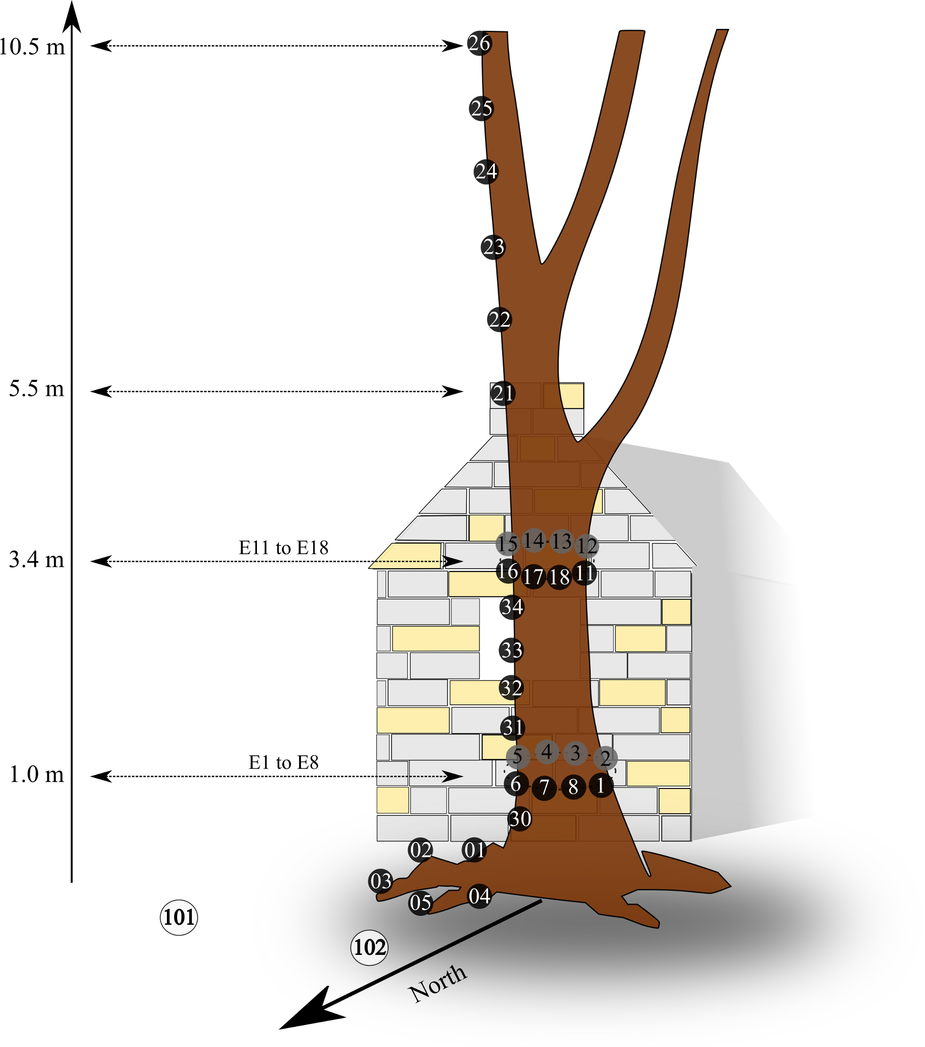
Figure 1: Schematic representation of the electrical acquisition protocol conducted on the Remungol poplar tree in 2003

The measuring instrument employed is a Keithley 2701 digital multimeter with an input impedance greater than 100 M$\Omega$, equipped with a relay matrix having 40 measurement channels controlled by acquisition software. Electric potential measurements are taken at all electrodes at a sampling interval of 1 minute. A UT time base was used, synchronized in real-time with the Frankfurt atomic clock. Both the computer and the multimeter are powered by a backup generator, mitigating interruptions due to brief electrical power line failures.

In Figure 2, we present an example of recorded data from both the roots, the trunk, and the branches during the period from October 1, 2002, to the end of June 2003. On the x-axis, which represents time, each tick corresponds to the first day of each month.

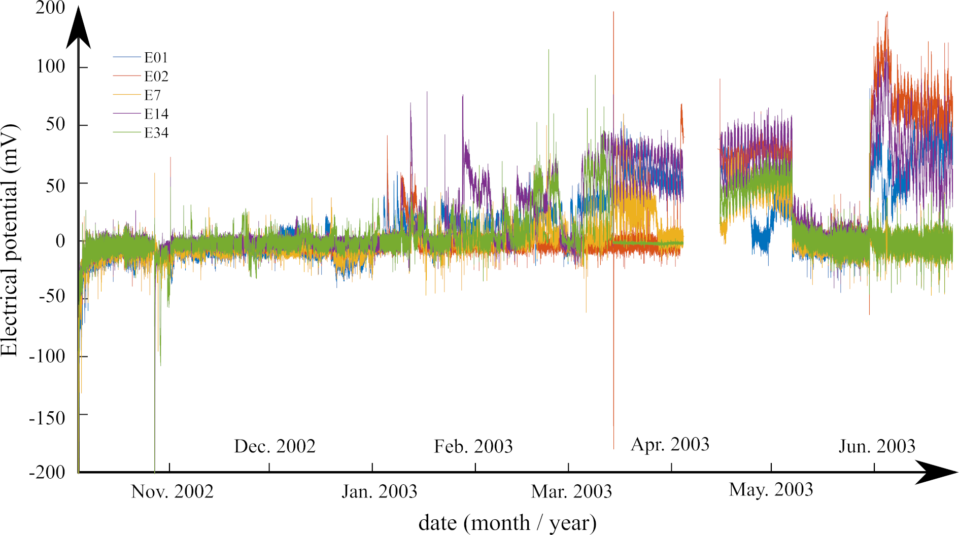
Figure 2: Illustration of some recorded potentials on both the roots and trunk of the poplar tree. One can observe the non-stationary nature of the potentials as well as data gaps in April 2003

Subsequently, we will present and analyze this time range, which is the longest with minimal gaps, covering transitions through each of the seasons. As illustrated in this figure, the electrical potentials, both in the roots, trunk, and branches, can vary by several hundred millivolts over the 320 days depicted. An activity (early) appears to commence in January 2023, reaching its peak during the summer of the same year. Clearly, the signals are not stationary, neither in the strict sense nor in the broader sense. Peaks of polarization are observed at times, and there is a gap in the data. These symptoms led us to choose Singular Spectrum Analysis as the method for analysis and extraction, which we will discuss later (Section 3).

Henceforth, when referring to the data from Gibert et al. ([16]), we will use the acronym RP (Remungol Poplar).

2.2 The new set up

In order to better understand the physics and physiology of trees, which were partially discussed in Gibert et al. ([16]), we have chosen to revisit the RP experiment and extend it by establishing a geophysical observatory for living trees at the Museum National d’Histoire Naturelle (MNHNo, Paris, France).

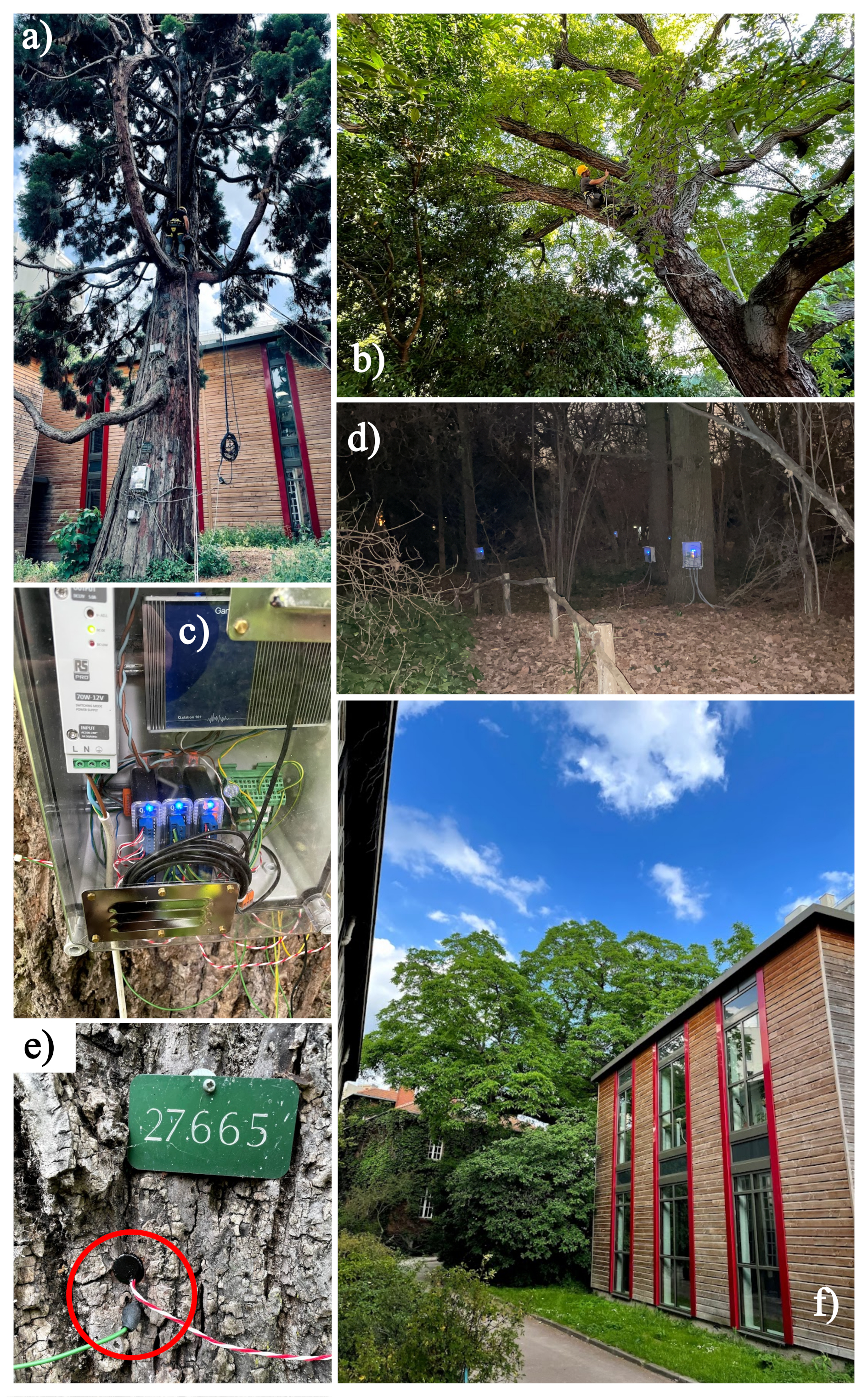
Figure 3: MNHN Observatory. a) Ongoing electrode placement on the trunk of the Sequoia. b) Ongoing electrode placement on the main branch of the Walnut tree. c) An example of a continuous electrical acquisition unit using Ganter modules. d) Nighttime photos of the instrumented 3 Oaks and 2 Hornbeams. The blue lights from the Gantner devices indicate the trees we are observing. e) In the red circle, an electrode (at the end of the green cable) inserted into the Walnut tree next to a thermal sensor (red and white cable). f) The Walnut tree and its canopy.

At MNHNo, we have currently instrumented 1 sequoia, 1 walnut, 1 cypress, 3 oaks, and 2 hornbeams: 2 conifers and 6 deciduous trees. The potentials are measured using stainless steel electrodes on both generators on the north side of the trunks and on crowns at various heights (from 1 to 9 meters) as well as on the branches of the trees. For the reference electrodes, we consistently use non-polarizable Petiau-type electrodes buried at a depth of approximately 1 meter. The trees are divided into 2 groups, with each group sharing the same non-polarizable electrode as a reference.We have added thermal measurements (Pt-100 and Pt-1000 probes) that record the temperature both inside and outside the trees, at various heights, as well as in the soil alongside the reference electrodes. We also monitor seismic activity as well as the variations in the inclination of trees (trunk and branches) over time. All measurements have been acquired and sampled at one-second intervals since 2019 using Gantner modular acquisition systems. These data acquisition now have significantly better performance than the Keitley 2701 used in 2003 : a high-impedance ($>$ 100 $M\Omega$) and a dynamic range of 24 bits capable of sampling up to 20 kHz per channel.

In Figure 3, we present a collage of photos showcasing our installations. Figure 3a shows the installation of the last electrode at 5 meters above the ground on the north side of the sequoia trunk. The white boxes on the trunk contain the Gantner acquisition system, as seen in Figure 3c. In Figure 3b, the installation of the first inclinometer on a branch at 3.5 meters above the ground is shown. On Figure 3c, the Gantner acquisition system (blue box at the top right) is accompanied by 3 electrical acquisition modules (at the bottom). Figure 3d displays a night photo of the acquisition boxes for the 3 oaks and 2 hornbeams. In Figure 3e, there is an example of combined electrical/thermal measurement in the sequoia at the same location. Finally, Figure 3f shows the canopy of the walnut tree captured between two research buildings.

Only the electrical measurements will be addressed in this study.

In Figure 4, examples of raw electrical measurements recorded between April 11, 2023, and May 11, 2023, are presented. The data are acquisitions from the 2 hornbeams at the top, the 3 oaks in the center, and a comparison between an oak and a hornbeam at the bottom. All 5 trees share the same reference no-polarizable electrode (Petiau), and the distance between the furthest individuals is approximately 10 meters. As observed, the order of magnitude of the potentials corresponds to those recorded in RP in 2003. Additionally, although diurnal oscillation is present in all individuals, within the same species, the variations in electrical amplitudes can range from 1 to 4 from one individual to another (see Figure 4 in the center). We will delve into these data in more detail later on.

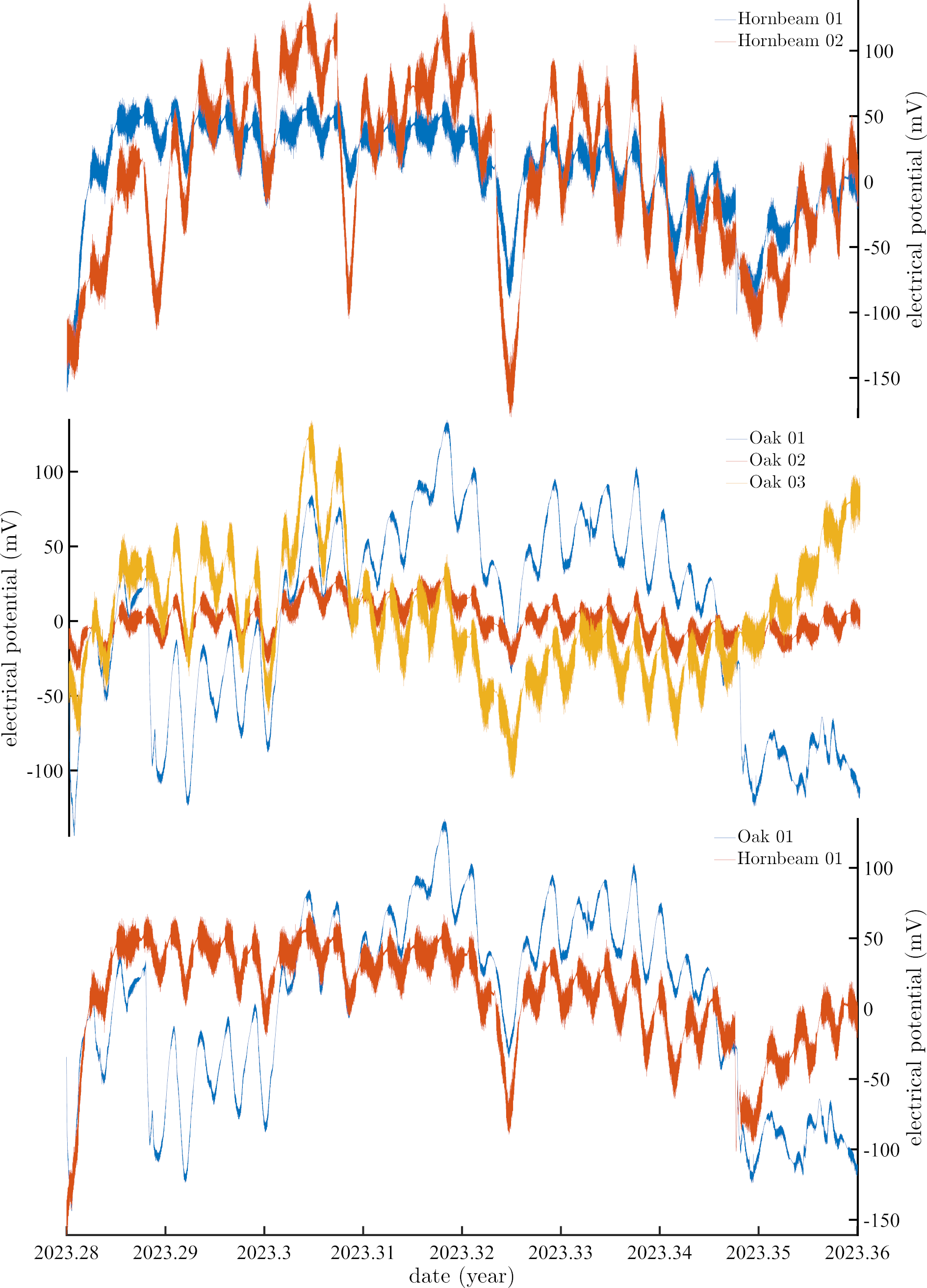
Figure 4: At the top, overlay of raw electrical signals measured at 1 meter above the ground in the trunks of the 2 hornbeams, north-facing. In the middle, overlay of raw electrical signals measured at 1 meter above the ground in the trunks of the 3 oaks, north-facing. At the bottom, overlay and comparison of raw electrical signals recorded by oak number 1 and hornbeam number 1.

3 The Singular Spectrum Analysis Method

The data, for which we have provided some examples (see Figures 2 and 2), correspond to a class of signals that are non-stationary in the strict sense and piecewise continuous. We are not in optimal conditions for their analysis in the Fourier sense (see[35, 36]). This is why we opted for the Singular Spectrum Analysis (SSA), which has historically been developed, in the field of paleoclimatology, to analyze this type of signals (see [37, 38]). We will present a brief overview of this method, and all the calculation details can be found in the reference work by Golyandina et al. ([39]).

SSA can be summarized in four steps. Let us consider a discrete time series ($\mathcal{X}_{N}$) of length N (N $>$ 2):

$$\mathcal{X}_{N}=(x_{1},\ldots,x_{N}).$$ (1)

Step 1: the Embedding Step

$\mathcal{X}_{N}$ is divided into $K$ segments of length $L$ in order to build a matrix X with the dimensions $K\times N$ where $K=N-L+1$ will condition our decomposition. This is the first ”tuning knob”. Integrating X yields a Hankel matrix.

$$\textbf{X}=\begin{pmatrix}x_{1}&x_{2}&x_{3}\cdots&x_{K}\\ x_{2}&x_{3}&x_{4}\cdots&x_{K+1}\\ x_{3}&x_{4}&x_{5}\cdots&x_{K+2}\\ \vdots&\vdots&\vdots\ddots&\vdots\\ x_{L}&x_{L+1}&x_{L+2}\cdots&x_{N}\end{pmatrix}$$ (2)

For further details regarding the properties of square matrices with constant values along ascending diagonals, such as Hankel or Toeplitz matrices, we invite the reader to explore the work of Lemmerling and Van Huffel ([40]).

Embedding consists in projecting the one-dimensional time series in a multidimensional space of series $\mathcal{X}_{N}$ such that vectors $X_{i}=(x_{i},\ldots,x_{i+L-1})^{t}$ belong to $\mathcal{R}^{L}$, where $K=N-L+1$. The parameter that controls the embedding is $L$, the size of the analyzing window, an integer between 2 and $N-1$. The Hankel matrix has a number of symmetry properties: its transpose $\textbf{X}^{t}$, called the trajectory matrix, has the dimension $K$. Embedding is a compulsory step in the analysis of nonlinear series. It consists formally in the empirical evaluation of all pairs of distances between two offset vectors, delayed (lagged) in order to calculate the correlation dimension of the series. This dimension is rather close to the fractal dimension of strange attractors that could generate that type of series. In this case, it is advised to select for the size of window $L$ very small values (and thus a very large $K$). On the contrary, for SSA, $L$ must be sufficiently large, so that each vector contains an important part of the information contained in the initial time series.

Step 2: Decomposition in Singular Values

Singular Value Decomposition (SVD, cf. [41]) of nonzero trajectory matrix X (dimensions $L\times K$ ) takes the following shape:

$$\textbf{X}=\sum_{i=1}^{d}\sqrt{\lambda_{i}}U_{i}V_{i}^{t}$$ (3)

where the eigenvalues $\lambda_{i}(i=1,\ldots,L)$ of matrix $\textbf{S}=\textbf{XX}^{T}$ are arranged in order of decreasing amplitudes. Eigenvectors $U_{i}$ and $V_{i}$ are given by :

$$V_{i}=\textbf{X}^{T}U_{i}/\sqrt{\lambda_{i}}$$ (4)

The $V_{i}$ form an orthonormal basis and are arranged in the same order as the $\lambda_{i}$. Let $\textbf{X}_{i}$ be a part of matrix X such that:

$$\textbf{X}_{i}=\sqrt{\lambda_{i}}U_{i}V_{i}^{t}.$$ (5)

Embedding matrix X can then be represented as a simple linear sum of elementary matrices $\textbf{X}_{i}$. If all eigenvalues are equal to 1, then decomposition of X into a sum of unitary matrices is :

$$\textbf{X}=\textbf{X}_{1}+\textbf{X}_{2}+\ldots+\textbf{X}_{d}$$ (6)

where $d$ is the rank of X ($d=\textrm{rank}\ \textbf{X}=max\{i|\lambda_{i}>0\}$). SVD allows one to write X as a sum of d unitary matrices, defined in a univocal way.

Let us now discuss the nature and the characteristics of the embedding matrix. Its rows and columns are sub-series of the original time series (or signal). The eigenvectors $U_{i}$ and $V_{i}$ have a time structure, and they can be considered as a representation of temporal data. Let X be a suite of $L$ lagged parts of ($\mathcal{X}$ and $X_{1},\ldots,X_{K}$) the linear basis of its eigenvectors. If we let:

$$Z_{i}=\sum_{i=1}^{d}\sqrt{\lambda_{i}}V_{i}$$ (7)

with $i=1,\ldots,d$, then the relation (5) can be written:

$$\textbf{X}=\sum_{i=1}^{d}U_{i}Z_{i}^{t}$$ (8)

that is, for the $j$th elementary matrix:

$$X_{j}=\sum_{i=1}^{d}z_{ji}U_{i}$$ (9)

where $z_{ji}$ is a component of vector $Z_{i}$ . This means that vector $Z_{i}$ is composed of the ith components of vector $X_{j}$. In the same way, if we let:

$$Y_{i}=\sum_{i=1}^{d}\sqrt{\lambda_{i}}U_{i}$$ (10)

we obtain for the transposed trajectory matrix:

$$X_{j}^{t}=\sum_{i=1}^{d}U_{i}Y_{i}^{t}$$ (11)

which corresponds to a representation of the K lagged vectors in the orthogonal basis ($V_{1}$, …, $V_{d}$). One sees why SVD is a very good choice for the analysis of the embedding matrix, since it provides two different geometrical descriptions.

Step 3: Reconstruction

As we have seen, $\textbf{X}_{i}$ matrices are unit matrices, and (as in the classical approach) one can “re-group” these matrices into a physically homogeneous quantity (or energetically homogeneous, etc…). This is the second ”tuning knob” of SSA. In order to regroup the unit matrices, one divides the set of indices $i\{1,\ldots,d\}$ into m disjoint subsets of indices $\{I_{1},\ldots,I_{m}\}$.

Let $I$ be the grouping of $p$ indices of $I=\{i_{1},i_{2},\ldots,i_{p}\}$; because (6) is linear, the resulting matrix $\textbf{X}_{I}$ that regroups indices I can be written:

$$\textbf{X}_{I}=\textbf{X}_{I1}+\textbf{X}_{I2}+\ldots+\textbf{X}_{Im}$$ (12)

This step is called regrouping the eigen triplets ($\lambda$, $U$ and $V$). In the limit case $m=d$, (12) becomes exactly (6), and we find again the unit matrices.

Next, how can one associate pairs of eigen triplets? This means separating the additive components of a time series. One must first consider the concept of separability.

Let $\mathcal{X}$ be the sum of two time series $\mathcal{X}^{(1)}$ and $\mathcal{X}^{(2)}$, such that $x_{i}=x_{i}^{(1)}+x_{i}^{(2)}$ for any $i\in[1,N]$. Let $L$ be the analyzing window (with fixed length), and $X$, $X^{(1)}$ and $X^{(2)}$ the embedding matrices of series $\mathcal{X},\mathcal{X}^{(1)}$ and $\mathcal{X}^{(2)}$. These two sub-series are separable (even weakly) in Equation (6) if there is a collection of indices $\mathcal{I}\subset\{1,\ldots,d\}$ such that $\textbf{X}^{(1)}=\sum_{i\in\mathcal{I}}\textbf{X}_{i}$, respectively, if there is a collection of indices such that $\textbf{X}^{(1)}=\sum_{i\not\in\mathcal{I}}\textbf{X}_{i}$. In the case when separability does exist, the contribution of $\textbf{X}^{(1)}$ for instance corresponds to the ratio of associated eigenvalues ($\sum_{i\in\mathcal{I}}\lambda_{i}$) to total eigenvalues ($\sum_{i=1}^{d}\lambda_{i}$).Still, in the case of relation (6), let $\mathcal{I}=\mathcal{I}_{1}$ be the set of indices corresponding to the first time series, with corresponding matrix $X_{\mathcal{I}_{1}}$. If both this matrix and that corresponding to the second time series ($\textbf{X}_{\mathcal{I}_{2}}=\textbf{X}-\textbf{X}_{\mathcal{I}_{1}}$) are close or identical to a Hankel matrix, then the time series are approximately or perfectly separable. So, regrouping SVD components can be summarized by the decomposition into several elementary matrices, whose structure must be as close as possible to a Hankel matrix of the initial trajectory matrix (this is true on paper only; in reality things are much more difficult).

Step 4:the Diagonal Mean (Hankelization)

The next, final step consists in going back to data space, that is, to calculate time series with length N associated with sub-matrices $\textbf{X}_{I}$. Let Y be a matrix with the dimensions $L\ast K$ and for each element $y_{i,j}$ we have $1\leqslant i\leqslant L$ and $1\leqslant j\leqslant K$. Let $L^{*}$ be the minimum and $K^{*}$ be the maximum. One always has $N=L+K-1$. Finally, let $y^{\ast}_{ij}=y_{ij}\ \textrm{if}\ L<K\ \textrm{and}\ y^{\ast}_{ij}=y_{ji}$ otherwise. The diagonal average applied to the $k$th index of time series y associated with matrix Y gives:

$$y_{k}=\left\{\begin{array}[]{cccc}\frac{1}{k}&\sum\limits_{m=1}^{k}y^{\ast}_{m,k-m+1}&\qquad 1\leqslant k\leqslant L^{\ast}\\ \frac{1}{L^{\ast}}&\sum\limits_{m=1}^{L^{\ast}}y^{\ast}_{m,k-m+1}&\qquad L^{\ast}\leqslant k\leqslant K^{\ast}\\ \frac{1}{N-K+1}&\sum\limits_{m=k-K\ast+1}^{N-K\ast+1}y^{\ast}_{m,k-m+1}&\qquad K^{\ast}\leqslant k\leqslant N^{\ast}\end{array}\right.$$ (13)

The relation (13) corresponds to the mean of the element on the antidiagonal $i+j=k+1$ of the matrix. For $k=1$, $y_{1}=y_{1,1}$. For $k=2$, $y_{2}=(y_{1,2}+y_{2,1})/2$, etc …

Thus, one reconstructs the time series with length $N$ from the matrices of step 3. If one applies the diagonal mean to unit matrices, then the series one obtains are called elementary series. Note that one can naturally extend the SSA of real signals to complex signals. One only has to replace all transposed marks with complex conjugates. As mentioned above, step 3 is the most difficult part.

We have chosen one approach among many others: iterative SSA. Since the relation (6) is linear, we can iterate the decomposition. We start with a small value of $L$ (we are looking for the longest period) that we increase until obtaining a quasi-Hankel matrix (step 3 and 3). We then extract the corresponding lowest frequency component that it subtracted from the original signal. We increase again the value of $L$ to find the next component (shortest period). The algorithm stops when no pseudo-cycle can be detected or extracted. In this way, we scan the series from low to high frequencies.

4 Data analysis and model

In a first step, we decompose the 2003 RP data using SSA for each of the 32 electrodes (see Figure 2). We observe that, in addition to diurnal and semi-diurnal oscillations ([16]), more than 70% of the data variability is carried by five major earth tides (see Table 1 and [42, 43]). Examples of extraction results are shown in Figure 5. For pedagogical reasons, we cannot overlay 32 curves on the same graph. The signals, once extracted by SSA, are regular enough for the calculation of a Fourier transform to make sense, in order to extract the nominal oscillation period of each of them.

Names	Periodicities	Magnitude ($cm^{2}/s^{2}$)	Origin
SSa	182.621 days	1909	solar declination
Mm	27.555 days	2163	lunar ellipticity
Mf	13.661 days	4099	lunar declination
Q1	26h 53m	1891	lunar ellipticity
O1	25h 49m	9876	main lunar wave
M1	24h 50m	1229	lunar ellipticity
P1	24h 04m	4600	main solar wave
K1	23h 56m	13902	solar and lunar declination (sideral day)
Q2	12h 39m	4556	lunar ellipticity
M2	12h 25m	23798	main lunar wave
S2	12h 00m	11081	main solar wave
K2	11h 58m	3015	solar and lunar declination

Table 1: List of main luni-solar tides. In the first column, their associated names, in the second column, the period, and finally, in the last column, the celestial origin of the respective period.

Presentation of some lunar-solar tides detected and extracted from the SP signals

In electrodes E1, E8, E32, and E34 (refer to our schematic in Figure 1), we have detected and extracted pseudo-cycles associated with the purely solar tide P₁(refer to our Table 1), which we present in Figure 5 (top-right). In Figure 6 (top-right), we show their respective Fourier spectra to determine the periodicities of these oscillations. These periodicities appear to be remarkably close, if not identical, to the ones obtained through calculations (refer to equations 01a and 01b), and we have indicated their theoretical values in the top-right corner of Figure 04b. Regarding the amplitudes, we observe a behavior that can only be attributed to the tree itself, as the variations in amplitudes are different at the same height ($\sim$1m) within the same crown (electrodes E1 and E8). We also note that these amplitudes evolve and seem to anticipate both solstices by approximately one month in all cases.

We change the set of four electrodes for Figures 5 (top-left) and 6 (top-left) to demonstrate the generality of our findings. The second component we have detected and extracted is a purely lunar tide, the K₁ tide. Once again, as shown in the period spectra in Figure 6 (top-left), the values of these periods are very close to the expected theoretical value of 23.93 hours. Similarly to what we observed for the S₁ tide, the amplitudes of the K₁ tide also appear to vary with the dates of solstices and equinoxes. The only difference here is that these variations are in phase with the mentioned dates. And as we observed for the previous tide, the potential increases from spring to reach its maximum in summer.

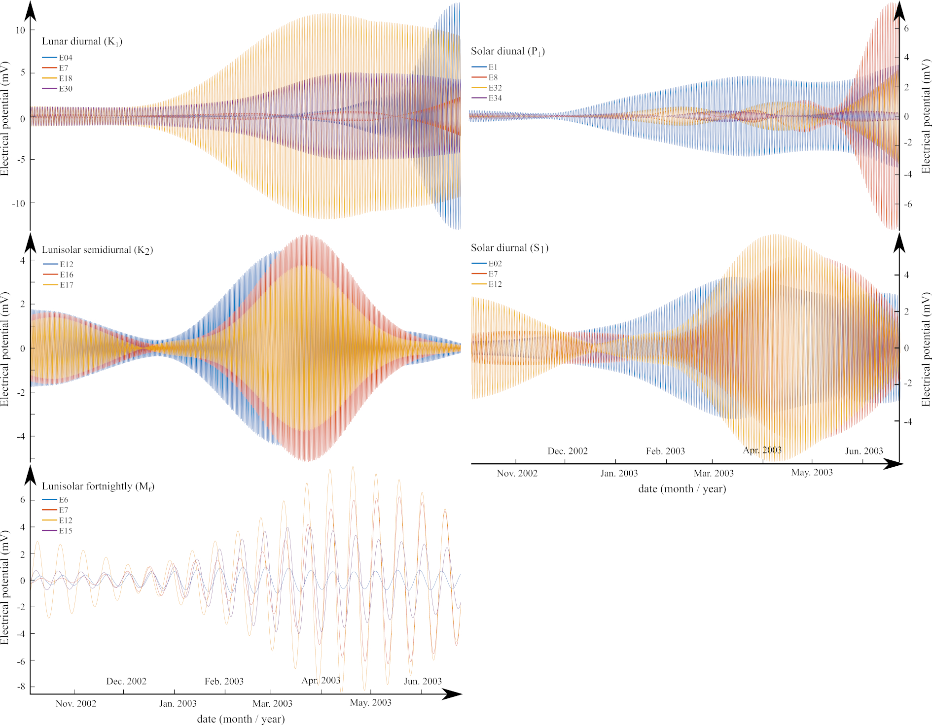
Figure 5: Top left: luni-solar tides K₁, extracted from electrodes E04, E7, E18, and E30.Top right: luni-solar tides P₁ extracted from electrodes E1, E8, E32, and E34. Middle left: luni-solar tides K₂ , extracted from electrodes E12, E16, E17. Middle right: luni-solar tides S₁ , extracted from electrodes E02, E7, E12. Bottom left: luni-solar tidess M_f, extracted by iSSA from electrodes E6, E7, E12,E13.

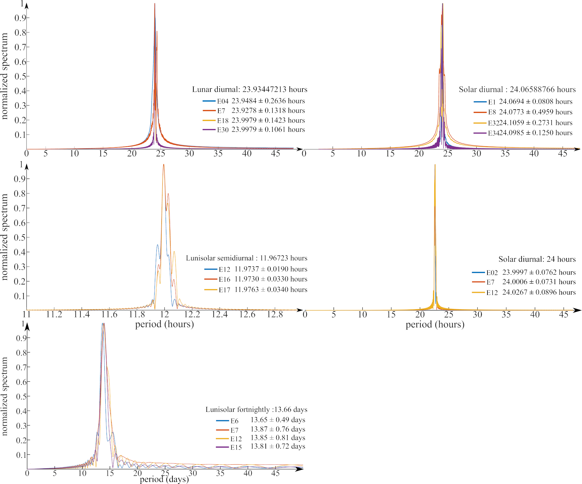
Figure 6: Fourier spectra corresponding to the signals presented in Figure 5.

The others components, Figures 5 (middle-left/right and bottom-left/right) and 6 (middle-left/right and bottom-left/right), present in sequence the waveforms and period spectra of the following lunar-solar tides: S₁, the fortnightly M_f, and K₂. Similar to the examples we have described before, the waveforms of these lunar-solar tides shown in Figures 5 and 6 are clearly modulated throughout the year, with a narrowing around the Winter solstice and a maximum amplitude shortly before the Summer solstice. These waveforms may not be in phase across different parts of the Remungol poplar tree (roots, trunk, branches), but in all cases, their calculated periods are very close to the expected values ($<$ 0.01$\%$).

For each of the 34 electrodes, it was possible to detect and extract between 7 luni-solar tides, which on average account for approximately 70% of the raw variance for each signal.

A mechanism

Let us then envision briefly an electrokinetic mechanism. Suppose the tree contains channels, taken as regular cylinders reaching going up to the top of the tree, in which the sap circulates. This circulation is not yet well understood (see [44, 45, 46, 47, 48, 5, 49]).

Let a channel of section $S$ of undetermined height. We will just make an order of magnitude computation of the pressure change in the channel due to the presence of a tidal forces of the Sun or (and) the Moon. Let us take the case of the Moon. $g$ being the gravity of the Earth (in fact an acceleration in $m.s^{-2}$, and we neglect here the effect of the Earth’s rotation; $g=9.81m.s^{-2}$ at the Earth’s surface).

The vertical component the Moon tide, always an attraction, is on the Earth’s surface given by the following relation,

$$0$$ (14)

$m$ is the mass of the Earth, $M$ the mass of the Moon, $r$ the mean radius, $R(t)$ the Earth-Moon distance, $\varphi$ the observation latitude. A similar relation gives the Solar tide, it is enough to replace the Earth-Moon distance by the Earth-Sun distance, and the mass of the Moon by that of the Sun. Ignoring the latitude factor in 14, and taking into account that $\dfrac{m}{M}=\dfrac{1}{80},\dfrac{r}{R(t)}\sim\dfrac{r}{R}\approx 1.662*10^{-2}$ it comes $\Delta g_{r}\sim 0.566*10^{-6}m.s^{-2}$ . Let us consider a channel in the tree of section $S$, and a slice of thickness $dz$; the lunar gravitational force acting on the slice is,

$$F_{grav}\sim 0.566*10^{-6}m.s^{-2}*\rho dzdS,$$ (15)

with the dimension of the force. We will take $\rho=10^{3}kg.m^{-3}$. In order to get an evaluation of the amount of pressure in the channel due to the gravitational force, we just write that the corresponding pressure gradient acting on the slice $dz$ is $S\dfrac{\partial p}{\partial z}dz$ is equal to the lunar gravitational force $F_{grav}$,

$$S\dfrac{\partial p}{\partial z}dz=0.566*10^{-6}m.^{s}{-2}*\rho Sdz\Rightarrow\dfrac{\partial p}{\partial z}=0.566*10^{-6}m.s^{-2}*\rho dz$$ (16)

Eventually, $\dfrac{\partial p}{dz}=0.566*10^{3}Pa.m^{-1}$. Now, it remains to estimate the electric potential gradient or electric field, in volt (V) per meter, using the electrokinetic coefficient $C$, $\dfrac{dV}{dz}=C\dfrac{\partial P}{\partial z}$ (dimension $\dfrac{V.m^{-1}}{Pa.m^{-1}}$). In principle, $C$ is determined by laboratory experiments,

$$C=\dfrac{\varepsilon\zeta}{\eta\sigma_{f}}$$ (17)

$\sigma_{f}$ is the conductivity of the fluid (sap), $\varepsilon$ is the conductivity of the fluid (sap), $\zeta$ is the $\zeta$-potential (here between the fluid and the wood wall of the channel) and $\eta$ the viscosity of the fluid. In fact we know very little about the value of $C$ relevant to the trees. The value of the electric field can be of the order of 10 $mV/m$ only if $C$ is of the order of 10V/Pa. Such value is large compared to the values found in literature, generally relevant to rocks.

A generalization across and within species

As we have already mentioned, tidal waves are waves with large geographical extensions; this means that they can be considered constant above MNHNo. We also decomposed the signals from our oaks and hornbeams using SSA (see Figure 4), and we only present the lunar-solar tide k1 (see Figure 7). The first observation here is that, regardless of the tree species and the individual within that same species, the cycles of earth-tides are in phase.

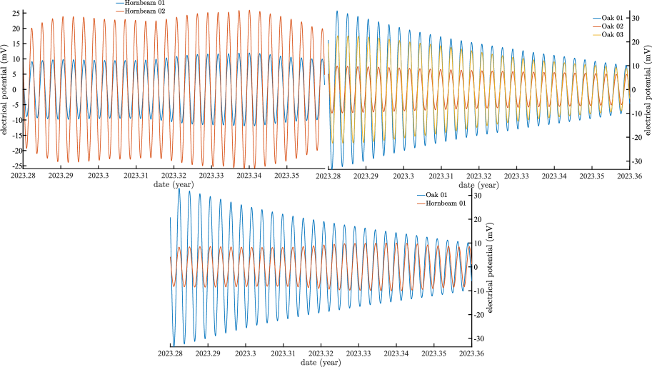
Figure 7: Lunar-solar tide K₁ during the period from April 11, 2023, to May 11, 2023, extracted: top left from our 2 hornbeams, top right from our 3 oaks. At the bottom, the superposition, over the same period, of the K₁ tides from the first oak (blue curve) and the first hornbeam (red curve)

The amplitudes during the months of April and May 2023, for all individuals, are on the order of $\pm$ 10 to 20 mV. These values are consistent with those of electrode E18 of RP (also on the North-facing trunk) during the same months (see Figure 5, top left, yellow curve). Thus, regardless of the period, both today and 20 years ago, measurements of electrical potentials on the trunks of three different species of deciduous trees (Poplar, Hornbeams, and Oaks) reveal, on one hand, comparable amplitudes of these potentials. On the other hand, the pseudo-cycles that compose them, such as the K₁ tide shown here, are in phase, independent of the individual. These electrical potentials, at least as shown here for the diurnal K₁, have been associated with the sap ascent through an electrokinetic effect (see [16]). The fact that all signals for this same potential are in phase and of the same order of magnitude, despite the differences in individuals (different sizes, different canopies, different physiology), leads us to believe that the observations we have made and the mechanism we propose are robust. For a significant part, the displacement of sap is due, as with all fluid masses outside the Earth, to the forcing effect of terrestrial tides.

5 Discussion

From a series of electrical SP data recorded on a Poplar tree in 2003 (see [16]), we propose to address the question of sap flow mechanism in trees. Today, for this mechanism, three sources are mentioned, which are not necessarily exclusive: capillarity, osmotic pressure, and evapotranspiration. We have discussed and critiqued the possibility of these mechanism in our introduction.

In a recent study (see [33]), we were able to measure the extent to which gravitational forces acting on Earth, through variations in its rotation speed and tilt, can influence the growth rates of tree rings in a Tibetan juniper forest for over 1000 years by modulating the incoming solar radiation. The growth rates of tree rings are linked to photosynthesis and, therefore, are also related to the flow of sap circulating in the xylem and phloem, which transport nutrients throughout the plant. At first order, like all fluids inside and on the surface of the Earth, the movement of this sap, regardless of its density, must be partially or entirely driven by lunar-solar tides, especially during the periods (¡18.6 years) that are of particular interest in this paper. Gibert et al. ([33]) emphasized that the sap flow and the recorded electrical signal were most likely linked by an electrokinetic phenomena. Therefore, in order to explain the movement of sap from a physics perspective, we are dealing here with a simple harmonic pumping phenomenon (see [17, 18]).

As illustrated in Figure 2, the continuously recorded electrical signals in trees are non-stationary signals in the strict sense. This inherently prevents the direct use of a Fourier transform to determine the periodicities (i.e., lunar-solar tides) that may compose them. Furthermore, measurement vagary sometimes lead to interruptions in the recording system, resulting in discontinuous data. That is why we chose the Singular Spectrum Analysis (SSA) method to analyze the measurements of the Remungol poplar. This method helps limit possible errors in the interpretation of traditional spectra.

In Figures 5 and 6, we presented the five main pseudo-periodicities extracted from the electrical potential data of the poplar. All of them correspond very precisely to periods of lunar-solar tides (P₁, K₁, S₁, M_f, and K₂, cf. our Table 1). The periods that we have extracted from the electrical signals, which serve as proxies for sap flow, are within 0.01% of the calculated lunar-solar tidal periods. This level of precision is remarkable and can typically only be achieved by expensive gravimeters costing tens of thousands of euros.

The sum of the extracted components, which we believe to be tidal components, generally accounts for more than 70% of the total variance in the recorded electrical signals.

If we examine in more detail the signals recorded in different areas of the Poplar tree (root, branch, trunk) for a given tide, we observe that the waveforms associated with these tides are not modulated in the same way. These amplitude modulations can be completely distinct from each other, as is the case for the tide and the electrodes E1, E8, E32, and E34 (cf. Figures 4). However, they can also be the same but phased in time. For example, we can observe that the patterns of the signals recorded by the electrodes E7 and E12 for the tide are the same but shifted by approximately 2 weeks (see Figures 5). Undoubtedly, the differences in amplitudes and phases observed in the recorded signals of the Poplar tree are likely to be related to its physiological response.

Based on these observations, we embarked on a mathematical resolution of the equations associated with the phenomenon that we believe to be responsible for the sap flow, aiming to evaluate the electrokinetic coefficient associated with the Poplar tree, similar to what is done in geophysics for rocks (see equation 17). We obtained a value of 10 V/Pa, which is generally ten times higher than the values measured in rocks. However, it should be noted that trees are not rocks, as we can by the picture of the xylem geometry in Figure 01, sap flow is not disrupted by any tortuosity, unlike in rocks. Furthermore, it is important to emphasize that sap is not water.

The question of the differences in amplitude modulations between different areas of the Poplar tree, as well as the question of the generality of our surprising results, led us to reproduce the same experiment in 2019 at the National Museum of Natural History, but this time on different tree species.

As we mentioned, we have three oak trees, two hornbeams, one sequoia, one cypress, and a walnut tree. We have only presented the observations we record on the oak and hornbeam trees for two reasons. The first reason is that, we have multiple individuals of the same species, allowing us to make intra-species comparisons. The second reason is that, these five trees are in the same location, sharing the same reference electrode. This allows us to consider inter-species comparisons, given that the spreading of gravitational waves is such that all Parisian trees will be affected simultaneously and with the same amplitude by earth tides.

As shown in Figures 4 and 7, the amplitudes and their variations differ significantly from one individual to another, which we could not estimate in the Remungol experiment. As we can see in Figure 13a and in more detail in Figure 7 (once the tide is extracted), on the one hand, the diurnal components of the three oak trees do not have the same electrical amplitudes (at the same electrode height), and on the other hand, longer-period oscillations appear on 2 of them (see Figure 4). We make the same observations for the hornbeams. However, what is confirmed by Figures 13c and 14c is that the components corresponding to the diurnal tide are perfectly in phase, from one individual to another, regardless of the species

Therefore, our hypothesis of the lunar-solar tide as the main driving force of sap flow is confirmed both by the richness of the observations and their incredible precision. The repeatability of these observations today with the trees at the MNHN Observatory confirms the results of Remungol and expands the research theme that we have yet to undertake, namely, that tree physiology appears to affect not the periods, but their modulations.

References

- [1] W. F. Pickard, “The ascent of sap in plants,” Progress in biophysics and molecular biology, vol. 37, pp. 181–229, 1981.
- [2] M. T. Tyree and S. Yang, “Water-storage capacity of thuja, tsuga and acer stems measured by dehydration isotherms: the contribution of capillary water and cavitation,” Planta, vol. 182, pp. 420–426, 1990.
- [3] S. Kang, X. Hu, P. Jerie, and J. Zhang, “The effects of partial rootzone drying on root, trunk sap flow and water balance in an irrigated pear (pyrus communis l.) orchard,” Journal of Hydrology, vol. 280, no. 1-4, pp. 192–206, 2003.
- [4] H. R. Brown, “The theory of the rise of sap in trees: some historical and conceptual remarks,” Physics in Perspective, vol. 15, pp. 320–358, 2013.
- [5] L. Li, Z.-L. Yang, A. M. Matheny, H. Zheng, S. C. Swenson, D. M. Lawrence, M. Barlage, B. Yan, N. G. McDowell, and L. R. Leung, “Representation of plant hydraulics in the noah-mp land surface model: Model development and multiscale evaluation,” Journal of Advances in Modeling Earth Systems, vol. 13, no. 4, p. e2020MS002214, 2021.
- [6] R. Munns and J. Passioura, “Effect of prolonged exposure to nacl on the osmotic pressure of leaf xylem sap from intact, transpiring barley plants,” Functional Plant Biology, vol. 11, no. 6, pp. 497–507, 1984.
- [7] U. Zimmermann, J. Zhu, F. Meinzer, G. Goldstein, H. Schneider, G. Zimmermann, R. Benkert, F. Thürmer, P. Melcher, D. Webb, et al., “High molecular weight organic compounds in the xylem sap of mangroves: Implications for long-distance water transport,” Botanica Acta, vol. 107, no. 4, pp. 218–229, 1994.
- [8] T. Scheenen, F. Vergeldt, A. Heemskerk, and H. Van As, “Intact plant magnetic resonance imaging to study dynamics in long-distance sap flow and flow-conducting surface area,” Plant physiology, vol. 144, no. 2, pp. 1157–1165, 2007.
- [9] K. H. Jensen, K. Berg-Sørensen, H. Bruus, N. M. Holbrook, J. Liesche, A. Schulz, M. A. Zwieniecki, and T. Bohr, “Sap flow and sugar transport in plants,” Reviews of modern physics, vol. 88, no. 3, p. 035007, 2016.
- [10] R. Munns, J. B. Passioura, T. D. Colmer, and C. S. Byrt, “Osmotic adjustment and energy limitations to plant growth in saline soil,” New Phytologist, vol. 225, no. 3, pp. 1091–1096, 2020.
- [11] A. Granier, “Evaluation of transpiration in a douglas-fir stand by means of sap flow measurements,” Tree physiology, vol. 3, no. 4, pp. 309–320, 1987.
- [12] D. Smith and S. Allen, “Measurement of sap flow in plant stems,” Journal of experimental Botany, vol. 47, no. 12, pp. 1833–1844, 1996.
- [13] R. Poyatos, V. Granda, R. Molowny-Horas, M. Mencuccini, K. Steppe, and J. Martínez-Vilalta, “Sapfluxnet: towards a global database of sap flow measurements,” Tree Physiology, vol. 36, no. 12, pp. 1449–1455, 2016.
- [14] R. Poyatos, V. Granda, V. Flo, M. A. Adams, B. Adorján, D. Aguadé, M. P. Aidar, S. Allen, M. S. Alvarado-Barrientos, K. J. Anderson-Teixeira, et al., “Global transpiration data from sap flow measurements: the sapfluxnet database,” Earth System Science Data Discussions, vol. 2020, pp. 1–57, 2020.
- [15] C. W. Thornthwaite, “An approach toward a rational classification of climate,” Geographical review, vol. 38, no. 1, pp. 55–94, 1948.
- [16] D. Gibert, J.-L. Le Mouël, L. Lambs, F. Nicollin, and F. Perrier, “Sap flow and daily electric potential variations in a tree trunk,” Plant Science, vol. 171, no. 5, pp. 572–584, 2006.
- [17] A. Maineult, Y. Bernabé, and P. Ackerer, “Detection of advected concentration and ph fronts from self-potential measurements,” Journal of Geophysical Research: Solid Earth, vol. 110, no. B11, 2005.
- [18] A. Maineult, E. Strobach, and J. Renner, “Self-potential signals induced by periodic pumping tests,” Journal of Geophysical Research: Solid Earth, vol. 113, no. B1, 2008.
- [19] V. Allegre, A. Maineult, F. Lehmann, F. Lopes, and M. Zamora, “Self-potential response to drainage–imbibition cycles,” Geophysical Journal International, vol. 197, no. 3, pp. 1410–1424, 2014.
- [20] P. S. Laplace, Traité de mécanique céleste. Imprimerie du Crapelet, 1823.
- [21] M. Milanković, Théorie mathématique des phénomènes thermiques produits par la radiation solaire. Gauthier-Villars et Cie, 1920.
- [22] F. Lopes, V. Courtillot, D. Gibert, J.-L. Le Mouël, and B. J.-B., “On pseudo-periodic perturbations of planetary orbits, and oscillations of earth’s rotation and revolution: Lagrange’s formulation,” arXiv preprint arXiv:2209.07213, 2022.
- [23] T. Narasimhan, B. Kanehiro, and P. Witherspoon, “Interpretation of earth tide response of three deep, confined aquifers,” Journal of Geophysical Research: Solid Earth, vol. 89, no. B3, pp. 1913–1924, 1984.
- [24] S. Rojstaczer and F. S. Riley, “Response of the water level in a well to earth tides and atmospheric loading under unconfined conditions,” Water Resources Research, vol. 26, no. 8, pp. 1803–1817, 1990.
- [25] H. Li, J. J. Jiao, M. Luk, and K. Cheung, “Tide-induced groundwater level fluctuation in coastal aquifers bounded by l-shaped coastlines,” Water Resources Research, vol. 38, no. 3, pp. 6–1, 2002.
- [26] S. Dumont, J.-L. Le Mouël, V. Courtillot, F. Lopes, F. Sigmundsson, D. Coppola, E. P. Eibl, and C. J. Bean, “The dynamics of a long-lasting effusive eruption modulated by earth tides,” Earth and Planetary Science Letters, vol. 536, p. 116145, 2020.
- [27] A. L. Lordi, M. C. Neves, S. Custódio, and S. Dumont, “Seasonal modulation of oceanic seismicity in the azores,” Frontiers in Earth Science, vol. 10, p. 995401, 2022.
- [28] S. L. Brantley, J. D. Kubicki, A. F. White, et al., Kinetics of water-rock interaction. Springer, 2008.
- [29] A. Scislewski and P. Zuddas, “Estimation of reactive mineral surface area during water–rock interaction using fluid chemical data,” Geochimica et Cosmochimica Acta, vol. 74, no. 24, pp. 6996–7007, 2010.
- [30] M. Barbera, P. Zuddas, D. Piazzese, E. Oddo, F. Lopes, P. Censi, and F. Saiano, “Accumulation of rare earth elements in common vine leaves is achieved through extraction from soil and transport in the xylem sap,” Communications Earth & Environment, vol. 4, no. 1, p. 291, 2023.
- [31] D. Gibert, V. Courtillot, S. Dumont, J. de Bremond d’Ars, S. Petrosino, P. Zuddas, F. Lopes, J.-B. Boulé, M. C. Neves, S. Custodio, et al., “On the external forcing of global eruptive activity in the past 300 years,” Frontiers in Earth Science, 2023.
- [32] V. Courtillot, J.-L. Le Mouël, F. Lopes, and D. Gibert, “On sea-level change in coastal areas,” Journal of Marine Science and Engineering, vol. 10, no. 12, p. 1871, 2022.
- [33] V. Courtillot, J.-B. Boulé, J.-L. Le Mouël, D. Gibert, P. Zuddas, A. Maineult, M. Gèze, and F. Lopes, “A living forest of tibetan juniper trees as a new kind of astro-geophysical observatory,” arXiv preprint arXiv:2306.11450, 2023.
- [34] G. Petiau and A. Dupis, “Noise, temperature coefficient, and long time stability of electrodes for telluric observations,” Geophysical Prospecting, vol. 28, no. 5, pp. 792–804, 1980.
- [35] J. F. Claerbout, Fundamentals of geophysical data processing, vol. 274. Citeseer, 1976.
- [36] S. M. Kay and S. L. Marple, “Spectrum analysis—a modern perspective,” Proceedings of the IEEE, vol. 69, no. 11, pp. 1380–1419, 1981.
- [37] R. Vautard and M. Ghil, “Singular spectrum analysis in nonlinear dynamics, with applications to paleoclimatic time series,” Physica D: Nonlinear Phenomena, vol. 35, no. 3, pp. 395–424, 1989.
- [38] R. Vautard, P. Yiou, and M. Ghil, “Singular-spectrum analysis: A toolkit for short, noisy chaotic signals,” Physica D: Nonlinear Phenomena, vol. 58, no. 1-4, pp. 95–126, 1992.
- [39] N. Golyandina, A. Korobeynikov, and A. Zhigljavsky, Singular spectrum analysis with R. Springer, 2018.
- [40] P. Lemmerling and S. Van Huffel, “Analysis of the structured total least squares problem for hankel/toeplitz matrices,” Numerical algorithms, vol. 27, pp. 89–114, 2001.
- [41] G. H. Golub and C. Reinsch, Singular value decomposition and least squares solutions. Springer, 1971.
- [42] J. Coulomb and G. Jobert, Traité de géophysique interne, Tome 1. 1973.
- [43] R. D. Ray and S. Y. Erofeeva, “Long-period tidal variations in the length of day,” Journal of Geophysical Research: Solid Earth, vol. 119, no. 2, pp. 1498–1509, 2014.
- [44] M. A. Zwieniecki, P. J. Melcher, T. S. Feild, and N. M. Holbrook, “A potential role for xylem–phloem interactions in the hydraulic architecture of trees: effects of phloem girdling on xylem hydraulic conductance,” Tree Physiology, vol. 24, no. 8, pp. 911–917, 2004.
- [45] C. W. Windt, F. J. Vergeldt, P. A. De Jager, and H. Van As, “Mri of long-distance water transport: a comparison of the phloem and xylem flow characteristics and dynamics in poplar, castor bean, tomato and tobacco,” Plant, Cell & Environment, vol. 29, no. 9, pp. 1715–1729, 2006.
- [46] M. A. Zwieniecki and N. M. Holbrook, “Confronting maxwell’s demon: biophysics of xylem embolism repair,” Trends in plant science, vol. 14, no. 10, pp. 530–534, 2009.
- [47] M. W. Vandegehuchte and K. Steppe, “Corrigendum to: Sap-flux density measurement methods: working principles and applicability,” Functional Plant Biology, vol. 40, no. 10, pp. 1088–1088, 2013.
- [48] Á. López-Bernal, L. Testi, and F. J. Villalobos, “A single-probe heat pulse method for estimating sap velocity in trees,” New Phytologist, vol. 216, no. 1, pp. 321–329, 2017.
- [49] G. Sakurai and S. J. Miklavcic, “On the efficacy of water transport in leaves. a coupled xylem-phloem model of water and solute transport,” Frontiers in Plant Science, vol. 12, p. 615457, 2021.