Scalable Structure Learning for Sparse Context-Specific Causal Systems

Abstract

Several approaches to graphically representing context-specific relations among jointly distributed categorical variables have been proposed, along with structure learning algorithms. While existing optimization-based methods have limited scalability due to the large number of context-specific models, the constraint-based methods are more prone to error than even constraint-based DAG learning algorithms since more relations must be tested. We present a hybrid algorithm for learning context-specific models that scales to hundreds of variables while testing no more constraints than standard DAG learning algorithms. Scalable learning is achieved through a combination of an order-based MCMC algorithm and sparsity assumptions analogous to those typically invoked for DAG models. To implement the method, we solve a special case of an open problem recently posed by Alon and Balogh. The method is shown to perform well on synthetic data and real world examples, in terms of both accuracy and scalability.

1 Introduction

We focus on the problem of structure learning (also known as causal discovery) for categorical data where one wishes to capture context-specific conditional independence relations in the data-generating distribution. Given a joint distribution ${\bf X}=(X_{1},\ldots,X_{p})$ and disjoint subsets $A,B,C\subset[p]:=\{1,\ldots,p\}$ with $A$ and $B$ nonempty, ${\bf X}_{A}$ is said to be conditionally independent of ${\bf X}_{B}$ given ${\bf X}_{C}$, written ${\bf X}_{A}\mathchoice{\mathrel{\hbox to0.0pt{$\displaystyle\perp$\hss}\mkern 2.0mu{\displaystyle\perp}}}{\mathrel{\hbox to0.0pt{$\textstyle\perp$\hss}\mkern 2.0mu{\textstyle\perp}}}{\mathrel{\hbox to0.0pt{$\scriptstyle\perp$\hss}\mkern 2.0mu{\scriptstyle\perp}}}{\mathrel{\hbox to0.0pt{$\scriptscriptstyle\perp$\hss}\mkern 2.0mu{\scriptscriptstyle\perp}}}{\bf X}_{B}|{\bf X}_{C}$ if $P({\bf x}_{A}|{\bf x}_{B},{\bf x}_{C})=P({\bf x}_{A}|{\bf x}_{C})$ for all marginal outcomes ${\bf x}_{A},{\bf x}_{B}$ and ${\bf x}_{C}$. Estimating CI relations entailed by jointly distributed categorical variables is well-known to reduce the number of parameters needed when performing inference tasks [Koller and Friedman, 2009]. This observation is one main motivation for estimating a DAG representation of a distribution. Given a directed acyclic graph $\operatorname{\mathcal{G}}=([p],E)$ with node set $[p]$ and edge set $E$, the distribution ${\bf X}$ is Markov to $\operatorname{\mathcal{G}}$ if

$$P({\bf x})=\prod_{i=1}^{p}P(x_{i}|{\bf x}_{\operatorname{pa}_{\operatorname{\mathcal{G}}}(i)})\,\,\,\,\mbox{$\forall\,{\bf x}=(x_{1},\ldots,x_{p})$,}$$ (1)

where $\operatorname{pa}_{\operatorname{\mathcal{G}}}(i)=\{k\in[p]:k\rightarrow i\in E\}$ denotes the set of parents of $i$ in $\operatorname{\mathcal{G}}$. The factorization reveals how CI relations entailed by the distribution reduce the number of parameters. When $\operatorname{\mathcal{G}}$ is sparse, the parent sets are small, reducing the number of parameters needed to represent the distribution as a product of conditional probabilities.

A DAG representation (i.e., a DAG $\operatorname{\mathcal{G}}$ to which the distribution is Markov) is thus a compact representation of the conditional probability table (CPT). Instead of storing the conditional probabilities $P(x_{i}|{\bf x}_{[i-1]})$ for all $i\in[p]$ and all outcomes ${\bf x}_{[i-1]}$, we store only enough to represent the factors $P(x_{i}|{\bf x}_{\operatorname{pa}_{\operatorname{\mathcal{G}}}(i)})$ for all $i$. When $\operatorname{\mathcal{G}}$ is sparse, this significantly reduces storage requirements for representing the distribution, and allows for speedy inference computations via message-passing [Koller and Friedman, 2009]. However, a DAG representation may obscure important relations that only hold for certain outcomes of a conditioning set. For disjoint subsets $A,B,C,S\subset[p]$ we say ${\bf X}_{A}$ is conditionally independent of ${\bf X}_{B}$ given ${\bf X}_{C}$ in the context ${\bf X}_{S}={\bf x}_{S}$ if

$$P({\bf x}_{A}|{\bf x}_{B},{\bf x}_{C},{\bf x}_{S})=P({\bf x}_{A}|{\bf x}_{C},{\bf x}_{S})\,\,\,\forall\,{\bf x}_{A},{\bf x}_{B},{\bf x}_{C}.$$

We denote this relation ${\bf X}_{A}\mathchoice{\mathrel{\hbox to0.0pt{$\displaystyle\perp$\hss}\mkern 2.0mu{\displaystyle\perp}}}{\mathrel{\hbox to0.0pt{$\textstyle\perp$\hss}\mkern 2.0mu{\textstyle\perp}}}{\mathrel{\hbox to0.0pt{$\scriptstyle\perp$\hss}\mkern 2.0mu{\scriptstyle\perp}}}{\mathrel{\hbox to0.0pt{$\scriptscriptstyle\perp$\hss}\mkern 2.0mu{\scriptscriptstyle\perp}}}{\bf X}_{B}|{\bf X}_{C},{\bf X}_{S}={\bf x}_{S}$ and call it a context-specific CI relation or CSI relation. Encoding CSI relations in the CPT captures more information at the price of additional computation and storage requirements, but it can also boost efficiency in inference [Boutilier et al., 1996]. By imposing sparsity requirements that limit the size of the sets $S$, one can strike a balance between additional detail and computational efficiency. In this paper, we present an algorithm for learning a graphical representation of sparse context-specific models that achieve this balance.

While a variety of optimization-based structure learning algorithms for context-specific models exist [Duarte and Solus, 2021, Hyttinen et al., 2018, Leonelli and Varando, 2023, Pensar et al., 2015], many of these methods strive for a broad generality in the CSI relations they can capture at the expense of only being able to learn models on few variables ($p\ll 100$). Constraint-based methods that generalize the PC algorithm for DAGs by analogous testing of CSI relations were also studied [Hyttinen et al., 2018]. While faster, these algorithms risk even more error than constraint-based DAG learners due to the increased number of constraints to test.

Our contributions include a hybrid approach combining constraint testing, an MCMC search and exact optimization. The constraint-based phase tests no more CI relations than a constraint-based DAG learner, limiting potential error propogation. We then use Markov chain Monte Carlo (MCMC) methods to estimate a maximum a posteriori variable ordering; a method shown to be highly effective in the DAG learning regime via the recent Benchpress platform for causal discovery method comparison [Rios et al., 2021]. To implement the MCMC algorithm, we solve a special case of a problem posed by Alon and Balogh [2023]. Finally, we utilize a novel context-specific sparsity assumption to efficiently perform exact optimization over all models with the optimal variable ordering. The algorithm scales ($p\gg 100$) while returning a sparse representation of the CPT with the same advantages for storage and inference as sparse DAG models. Scalability is demonstrated through both complexity bounds (Theorem 2) and evaluation on synthetic data and real world examples. The experiments also show the method achieving a high level of accuracy. Our implementation and experimental analysis are publicly available as part of an open-source software package: CStrees.

2 Related Work

Several models for context-specific relations exist, ranging from relatively minimal assumptions yielding subtle extensions of DAG models to broad attempts at capturing many CSI relations. The former models include Bayesian multinets [Geiger and Heckerman, 1996] and similarity networks [Heckerman, 1990] which introduce a single variable to distinguish between contexts, called the hypothesis variable or distinguished node. These models allow for CSI relations where the contexts are limited to the scope of the hypothesis variable. They possess many of the efficiencies of DAG models but are limited in the CSI relations they capture.

At the other extreme are staged trees, introduced by Smith and Anderson [2008], capable of encoding a wealth of CSI relations. However, the graphical representation of a staged tree typically lacks interpretability since the size of the graph grows on the order of $2^{p}$ for even binary variables. Chain Event Graphs [Smith and Anderson, 2008] reduce the staged tree representation, but can still be difficult to interpret.

To overcome scalability problems, subfamilies of staged trees were studied and associated structure learning methods were proposed. Leonelli and Varando [2022] proposed a method that first estimates a DAG with bounded in-degree using classical causal discovery methods and then greedily optimizes the staging, which represents the CSI relations in the model. The method is relatively efficient due to the sparsity constraints imposed by bounds on the parent sets in the DAG. Other staged tree algorithms instead limit variable ordering without the use of a DAG [Strong and Smith, 2022]. However, these methods inevitably use a greedy search to learn CSI-relations which risks error that is avoided by our exact optimization approach to this step. Other staged tree algorithms [Leonelli and Varando, 2023] achieve efficiency only by searching over a fixed variable ordering, which is subject to misspecification. Our MCMC approach to order search is known to be effective in DAG learning [Friedman and Koller, 2003] and allows us to efficiently determine an optimal variable ordering. Our learned models also admit more compact and interpretable representations.

Between the two extremes are the Labeled DAGs (LDAGs) [Pensar et al., 2015] that are more interpretable than staged-trees but also capture more context-specific information than similarity networks. LDAGs are context specific models that encode pairwise CSI relations $X_{i}\mathchoice{\mathrel{\hbox to0.0pt{$\displaystyle\perp$\hss}\mkern 2.0mu{\displaystyle\perp}}}{\mathrel{\hbox to0.0pt{$\textstyle\perp$\hss}\mkern 2.0mu{\textstyle\perp}}}{\mathrel{\hbox to0.0pt{$\scriptstyle\perp$\hss}\mkern 2.0mu{\scriptstyle\perp}}}{\mathrel{\hbox to0.0pt{$\scriptscriptstyle\perp$\hss}\mkern 2.0mu{\scriptscriptstyle\perp}}}X_{j}|{\bf X}_{\operatorname{pa}_{\operatorname{\mathcal{G}}}(i)\setminus j}={\bf x}_{\operatorname{pa}_{\operatorname{\mathcal{G}}}(i)\setminus j}$ where $j\rightarrow i$ is an edge in a DAG representation of the distribution; i.e., they encode CSI relations that represent a single edge vanishing for a specified context of the other parents of $i$. Such models have proven useful, as they are more amenable to both structure learning [Hyttinen et al., 2018] and causal inference. In the latter case, LDAGs help capture additional causal relations from only observational data [Tikka et al., 2019] by identifying additional essential arrows [Andersson et al., 1997] in the DAG.

Hyttinen et al. [2018] explored constraint-based and exact optimization-based methods for learning LDAGs. While the constraint-based methods can scale under sparsity constraints, the algorithms run analogous to the PC algorithm [Spirtes and Glymour, 1991] but test CSI relations over all possible contexts. This requires more tests that may lead to errors in addition to those of the classical PC algorithm. Our proposed method tests no more CI relations than classical PC, limiting the possibility for error. Hyttinen et al. [2018] also show how exact optimization methods can be done using local score computations for LDAGs, but they note that these methods are generally infeasbile for distributions with more than four variables (although they include an example on $37$ nodes with variables on up to four states with a rather impressive run time of only seven hours on a modern desktop computer). Pensar et al. [2015] present a non-reversible Markov chain approach for learning LDAGs that blends stochastic and greedy search. This method potentially achieves higher accuracy over the constraint-based methods. However, Hyttinen et al. [2018] note that the blending of stochastic and greedy searches necessitates careful parameter tuning to avoid overfitting and obtain accuracy gains over constraint-based methods.

A potential downside to LDAGs is that the models are specified by pairwise CSI relations. DAG models are compositional [Sadeghi and Lauritzen, 2014], meaning that $X_{i}\mathchoice{\mathrel{\hbox to0.0pt{$\displaystyle\perp$\hss}\mkern 2.0mu{\displaystyle\perp}}}{\mathrel{\hbox to0.0pt{$\textstyle\perp$\hss}\mkern 2.0mu{\textstyle\perp}}}{\mathrel{\hbox to0.0pt{$\scriptstyle\perp$\hss}\mkern 2.0mu{\scriptstyle\perp}}}{\mathrel{\hbox to0.0pt{$\scriptscriptstyle\perp$\hss}\mkern 2.0mu{\scriptscriptstyle\perp}}}X_{j}|{\bf X}_{C}$ and $X_{i}\mathchoice{\mathrel{\hbox to0.0pt{$\displaystyle\perp$\hss}\mkern 2.0mu{\displaystyle\perp}}}{\mathrel{\hbox to0.0pt{$\textstyle\perp$\hss}\mkern 2.0mu{\textstyle\perp}}}{\mathrel{\hbox to0.0pt{$\scriptstyle\perp$\hss}\mkern 2.0mu{\scriptstyle\perp}}}{\mathrel{\hbox to0.0pt{$\scriptscriptstyle\perp$\hss}\mkern 2.0mu{\scriptscriptstyle\perp}}}X_{k}|{\bf X}_{C}$ imply $X_{i}\mathchoice{\mathrel{\hbox to0.0pt{$\displaystyle\perp$\hss}\mkern 2.0mu{\displaystyle\perp}}}{\mathrel{\hbox to0.0pt{$\textstyle\perp$\hss}\mkern 2.0mu{\textstyle\perp}}}{\mathrel{\hbox to0.0pt{$\scriptstyle\perp$\hss}\mkern 2.0mu{\scriptstyle\perp}}}{\mathrel{\hbox to0.0pt{$\scriptscriptstyle\perp$\hss}\mkern 2.0mu{\scriptscriptstyle\perp}}}X_{j,k}|{\bf X}_{C}$. This allows us to pass from the observed pairwise CI relations $X_{i}\mathchoice{\mathrel{\hbox to0.0pt{$\displaystyle\perp$\hss}\mkern 2.0mu{\displaystyle\perp}}}{\mathrel{\hbox to0.0pt{$\textstyle\perp$\hss}\mkern 2.0mu{\textstyle\perp}}}{\mathrel{\hbox to0.0pt{$\scriptstyle\perp$\hss}\mkern 2.0mu{\scriptstyle\perp}}}{\mathrel{\hbox to0.0pt{$\scriptscriptstyle\perp$\hss}\mkern 2.0mu{\scriptscriptstyle\perp}}}X_{j}|{\bf X}_{\operatorname{pa}_{\operatorname{\mathcal{G}}}(i)}$ for all $j\in[i-1]\setminus\operatorname{pa}_{\operatorname{\mathcal{G}}}(i)$ to the relations $X_{i}\mathchoice{\mathrel{\hbox to0.0pt{$\displaystyle\perp$\hss}\mkern 2.0mu{\displaystyle\perp}}}{\mathrel{\hbox to0.0pt{$\textstyle\perp$\hss}\mkern 2.0mu{\textstyle\perp}}}{\mathrel{\hbox to0.0pt{$\scriptstyle\perp$\hss}\mkern 2.0mu{\scriptstyle\perp}}}{\mathrel{\hbox to0.0pt{$\scriptscriptstyle\perp$\hss}\mkern 2.0mu{\scriptscriptstyle\perp}}}{\bf X}_{[i-1]\setminus\operatorname{pa}_{\operatorname{\mathcal{G}}}(i)}|{\bf X}_{\operatorname{pa}_{\operatorname{\mathcal{G}}}(i)}$ that define the factorization in (1). It is not known if LDAGs are compositional, but given that they represent a very large family of models, this seems unlikely as general discrete distributions are not compositional [Studeny, 2006].

Recently, a family of submodels of LDAGs, called CStrees, were isolated and studied by Duarte and Solus [2021]. Instead of pairwise CSI relations, CStrees are defined via a relaxation of the factorization in (1) (see Section 3). CStrees are submodels of LDAGs and all DAG models are CStree models. Hence, CStrees possess the desirable features of LDAGs while being somewhat closer to Bayesian networks. Since CStrees are defined according to a factorization, they admit natural opportunities to impose novel context-specific sparsity constraints that easily generalize those used for DAG models (bounded number of parents). These sparsity constraints allow for easy model enumeration (Theorem 1), which is necessary for computing model scores typically used in MCMC algorithms. For these reasons, our proposed structure learning algorithm is designed to estimate sparse CStree models. In Section 4, we take advantage of the features of CStrees to give a fast structure learning method whose estimates have the desirable properties of LDAGs while also capturing more information than a DAG.

3 Models

The models we study are a subfamily of LDAGs called CStrees. They admit the CStree representations of Duarte and Solus [2021] as well as the LDAG representation of Pensar et al. [2015]. While LDAG representations will be used to present an interpretabile model representation, the CStree structure will be used to achieve fast structure learning.

A CStree model is defined for a collection of jointly distributed categorical variables $(X_{1},\ldots,X_{p})$, and it is simply an ordered pair $\mathcal{T}=(\pi,\mathbf{s})$ where $\pi$ is a variable ordering and $\mathbf{s}$ is a collection of sets. Suppose $X_{i}$ has state space $[d_{i}]$ for $d_{1},\ldots,d_{p}>1$ and ${\bf X}$ assumes the product measure with state space $\mathcal{X}=\prod_{i=1}^{p}[d_{i}]$. For $S\subset[p]$ we let ${\bf X}_{S}=(X_{i}:i\in S)$ denote the marginal distribution on the variables with indices in $S$, and we denote its state space with $\mathcal{X}_{S}$. Let $\pi=\pi_{1}\pi_{2}\cdots\pi_{p}$ denote a total ordering of the indices $[p]$ and consider CSI relations of the form

$$X_{\pi_{i}}\mathchoice{\mathrel{\hbox to0.0pt{$\displaystyle\perp$\hss}\mkern 2.0mu{\displaystyle\perp}}}{\mathrel{\hbox to0.0pt{$\textstyle\perp$\hss}\mkern 2.0mu{\textstyle\perp}}}{\mathrel{\hbox to0.0pt{$\scriptstyle\perp$\hss}\mkern 2.0mu{\scriptstyle\perp}}}{\mathrel{\hbox to0.0pt{$\scriptscriptstyle\perp$\hss}\mkern 2.0mu{\scriptscriptstyle\perp}}}{\bf X}_{[\pi_{1}:\pi_{i-1}]\setminus S}|{\bf X}_{S}={\bf x}_{S}$$ (2)

for some context ${\bf x}_{S}\in\mathcal{X}_{S}$ where $S\subset\{\pi_{1},\ldots,\pi_{i-1}\}$. To this relation, we associate the set $\mathcal{S}_{\pi,i}({\bf x}_{S})$ of all marginal outcomes ${\bf x}_{\pi_{1}:\pi_{i-1}}\in\mathcal{X}_{[\pi_{1}:\pi_{i-1}]}$ that equal the context ${\bf x}_{S}$ when restricted to the values with indices in $S$. Let $\mathcal{C}_{\pi,i}$ denote a set of CSI relations of the form (2) for a given $i\in[p]$ and the ordering $\pi$. Consider $\mathcal{C}_{\mathcal{T}}=\mathcal{C}_{\pi,1}\cup\cdots\cup\mathcal{C}_{\pi,p}$, with one set $\mathcal{C}_{\pi,i}$ for each $i\in[p]$. We obtain a set of distributions defined by the relations in $\mathcal{C}_{\mathcal{T}}$:

$$\mathcal{M}(\mathcal{T})=\{{\bf X}:{\bf X}\mbox{ entails all relations in $\mathcal{C}_{\mathcal{T}}$}\}.$$

If for each $C_{\pi,i}$,

$$\mathbf{s}_{i}=\{\mathcal{S}_{\pi,i}({\bf x}_{S}):X_{\pi_{i}}\mathchoice{\mathrel{\hbox to0.0pt{$\displaystyle\perp$\hss}\mkern 2.0mu{\displaystyle\perp}}}{\mathrel{\hbox to0.0pt{$\textstyle\perp$\hss}\mkern 2.0mu{\textstyle\perp}}}{\mathrel{\hbox to0.0pt{$\scriptstyle\perp$\hss}\mkern 2.0mu{\scriptstyle\perp}}}{\mathrel{\hbox to0.0pt{$\scriptscriptstyle\perp$\hss}\mkern 2.0mu{\scriptscriptstyle\perp}}}{\bf X}_{[\pi_{1}:\pi_{i-1}]\setminus S}|{\bf X}_{S}={\bf x}_{S}\in\mathcal{C}_{\pi,i}\}$$

is a set of disjoint subsets of $\mathcal{X}_{[\pi_{1}:\pi_{i-1}]}$, we call the model $\mathcal{M}(\mathcal{T})$ a CStree model for the CStree $\mathcal{T}=(\pi,\mathbf{s})$ where $\mathbf{s}=\bigcup_{i\in[p]}\mathbf{s}_{i}$. Let $\operatorname{ms}(\mathbf{s}_{i})$ denote the maximum size of a set $S$ such that there is a relation (2) with ${\bf X}_{X}={\bf x}_{S}$ in $\mathcal{C}_{\pi,i}$.

A distribution ${\bf X}$ is Markov to $\mathcal{T}=(\pi,\mathbf{s})$ if ${\bf X}\in\mathcal{M}(\mathcal{T})$. The use of the word “Markov” suggests a factorization of $P({\bf x})$ analogous to that for DAGs in (1). Indeed, given $i\in[p]$ each outcome ${\bf x}_{[\pi_{1}:\pi_{i-1}]}\in\mathcal{S}_{\pi,i}({\bf x}_{S})$ can be mapped to the set of variables $S$ indexing the context ${\bf x}_{S}$. Let

$$\operatorname{pa}_{\mathcal{T}}:\bigcup_{i\in[p]}\mathcal{X}_{[\pi_{1}:\pi_{i-1}]}\rightarrow\{S:S\subseteq[p]\}$$

denote this map. Then ${\bf X}$ is Markov to $\mathcal{T}$ if and only if

$$P({\bf x})=\prod_{i=1}^{p}P(x_{\pi_{i}}|{\bf x}_{\operatorname{pa}_{\mathcal{T}}({\bf x}_{\pi_{1}:\pi_{i-1}})})$$

for all ${\bf x}\in\mathcal{X}$. The set ${\operatorname{pa}_{\mathcal{T}}({\bf x}_{\pi_{1}:\pi_{i-1}})}$ can be viewed as the context-specific parents of the node ${\bf x}_{\pi_{1}:\pi_{i-1}}$. If $\mathbf{s}_{i}=\{\mathcal{S}_{\pi,i}({\bf x}_{P_{i}}):{\bf x}_{P_{i}}\in\mathcal{X}_{P_{i}}\}$ for some set $P_{i}$ for each $i$ then the above factorization reduces to (1), recovering DAG models. So CStrees are a generalization of DAG models.

The model defining relations $\mathcal{C}_{\mathcal{T}}$ may be graphically represented by a rooted tree with colored vertices. Consider a rooted tree $\mathcal{T}$ with vertex set $\{r\}\cup\bigcup_{i\in[p]}\mathcal{X}_{[i]}$ and edges ${\bf x}_{\pi_{1}:\pi_{i-1}}\rightarrow{\bf x}_{\pi_{1}:\pi_{i-1}}x_{\pi_{i}}$ for all pairs ${\bf x}_{\pi_{1}:\pi_{i-1}}\in\mathcal{X}_{[\pi_{1}:\pi_{i-1}]}$ and $x_{\pi_{i}}\in\mathcal{X}_{\pi_{i}}$ and $r\rightarrow x_{\pi_{1}}$ for all $x_{\pi_{1}}\in\mathcal{X}_{\pi_{1}}$. We color the nodes in each set $\mathcal{S}_{\pi,i}({\bf x}_{S})$ the same, using a distinct color for each set. This colored tree then encodes exactly the defining CSI relations $\mathcal{C}_{\mathcal{T}}$ (and hence the distribution’s factorization).

Figure 1: A CStree $\mathcal{T}$ for variable ordering $\pi=1234$.

Example 1.

For example, Let $\pi=1234$ be the variable ordering, and consider the set of CSI relations

$$\begin{split}\mathcal{C}_{\mathcal{T}}=\{&X_{2}\mathchoice{\mathrel{\hbox to0.0pt{$\displaystyle\perp$\hss}\mkern 2.0mu{\displaystyle\perp}}}{\mathrel{\hbox to0.0pt{$\textstyle\perp$\hss}\mkern 2.0mu{\textstyle\perp}}}{\mathrel{\hbox to0.0pt{$\scriptstyle\perp$\hss}\mkern 2.0mu{\scriptstyle\perp}}}{\mathrel{\hbox to0.0pt{$\scriptscriptstyle\perp$\hss}\mkern 2.0mu{\scriptscriptstyle\perp}}}X_{1},\\ &X_{3}\mathchoice{\mathrel{\hbox to0.0pt{$\displaystyle\perp$\hss}\mkern 2.0mu{\displaystyle\perp}}}{\mathrel{\hbox to0.0pt{$\textstyle\perp$\hss}\mkern 2.0mu{\textstyle\perp}}}{\mathrel{\hbox to0.0pt{$\scriptstyle\perp$\hss}\mkern 2.0mu{\scriptstyle\perp}}}{\mathrel{\hbox to0.0pt{$\scriptscriptstyle\perp$\hss}\mkern 2.0mu{\scriptscriptstyle\perp}}}X_{1}|X_{2}=1,\\ &X_{4}\mathchoice{\mathrel{\hbox to0.0pt{$\displaystyle\perp$\hss}\mkern 2.0mu{\displaystyle\perp}}}{\mathrel{\hbox to0.0pt{$\textstyle\perp$\hss}\mkern 2.0mu{\textstyle\perp}}}{\mathrel{\hbox to0.0pt{$\scriptstyle\perp$\hss}\mkern 2.0mu{\scriptstyle\perp}}}{\mathrel{\hbox to0.0pt{$\scriptscriptstyle\perp$\hss}\mkern 2.0mu{\scriptscriptstyle\perp}}}X_{2}|X_{1,3}=(1,1),\\ &X_{4}\mathchoice{\mathrel{\hbox to0.0pt{$\displaystyle\perp$\hss}\mkern 2.0mu{\displaystyle\perp}}}{\mathrel{\hbox to0.0pt{$\textstyle\perp$\hss}\mkern 2.0mu{\textstyle\perp}}}{\mathrel{\hbox to0.0pt{$\scriptstyle\perp$\hss}\mkern 2.0mu{\scriptstyle\perp}}}{\mathrel{\hbox to0.0pt{$\scriptscriptstyle\perp$\hss}\mkern 2.0mu{\scriptscriptstyle\perp}}}X_{2}|X_{1,3}=(1,0),\\ &X_{4}\mathchoice{\mathrel{\hbox to0.0pt{$\displaystyle\perp$\hss}\mkern 2.0mu{\displaystyle\perp}}}{\mathrel{\hbox to0.0pt{$\textstyle\perp$\hss}\mkern 2.0mu{\textstyle\perp}}}{\mathrel{\hbox to0.0pt{$\scriptstyle\perp$\hss}\mkern 2.0mu{\scriptstyle\perp}}}{\mathrel{\hbox to0.0pt{$\scriptscriptstyle\perp$\hss}\mkern 2.0mu{\scriptscriptstyle\perp}}}X_{2}|X_{1,3}=(0,1)\}.\end{split}$$

The context defining the CSI relation of the form (2) for variable $X_{3}$ is $x_{2}=1$. Hence, the nodes $(0,1)$ and $(1,1)$ are the same color (green) in the tree $\mathcal{T}$ in Figure 1. For variable $X_{4}$, we have CSI relations defined by contexts ${\bf x}_{1,3}=(1,1)$, ${\bf x}_{1,3}=(1,0)$ and ${\bf x}_{1,3}=(0,1)$, which respectively correspond to the colored sets of nodes $\{(1,0,1),(1,1,1)\}$ (blue), $\{(1,0,0),(1,1,0)\}$ (orange) and $\{(0,0,1),(0,1,1)\}$ (red) in $\mathcal{T}$. Similarly, the context defining the relation $X_{2}\mathchoice{\mathrel{\hbox to0.0pt{$\displaystyle\perp$\hss}\mkern 2.0mu{\displaystyle\perp}}}{\mathrel{\hbox to0.0pt{$\textstyle\perp$\hss}\mkern 2.0mu{\textstyle\perp}}}{\mathrel{\hbox to0.0pt{$\scriptstyle\perp$\hss}\mkern 2.0mu{\scriptstyle\perp}}}{\mathrel{\hbox to0.0pt{$\scriptscriptstyle\perp$\hss}\mkern 2.0mu{\scriptscriptstyle\perp}}}X_{1}$ is the empty context ${\bf x}_{\emptyset}$ where we assume ${\bf x}_{\emptyset}$ is a subvector of any vector of outcomes. Thus, $\mathcal{S}({\bf x}_{\emptyset})=\mathcal{X}_{1}=\{0,1\}$, and so the two nodes $(0)$ and $(1)$ are colored the same (yellow), representing this CI relation. The white nodes are uncolored since they do not lie in any of the sets $\mathcal{S}({\bf x}_{S})$ for any of these contexts. $\blacksquare$

Figure 2: LDAG representation of the CStree in Figure 1.

The tree $\mathcal{T}$ in Figure 1 is an example of a staged tree representation of a context-specific model, and it shows why staged trees are difficult to interpret even for very few variables. As the number of variables and state spaces for each variables grow, we simply cannot draw or interpret such a graphical representation.

In the language of the staged tree literature, we call the set $\mathcal{S}_{\pi,i}({\bf x}_{S})$ a stage, ${\bf x}_{S}$ its stage-defining context and $S$ its set of context variables. Note that each stage corresponds to a set of colored nodes in $\mathcal{T}$. We call the set of outcomes $\mathcal{X}_{[i]}$ level $i$ of $\mathcal{T}=(\pi,\mathbf{s})$ and $\mathbf{s}_{i}$ a staging of level $i$. The set $\mathbf{s}$ is a staging of the tree. The stage $s=\mathcal{S}_{\pi,i}({\bf x}_{S})\in\mathbf{s}_{i}$ corresponds to a conditional probability $P(X_{\pi_{i}}|{\bf x}_{S})$ used in the factorization (3). We parametrize this conditional distribution with $\mathbf{\theta}_{\pi_{i},s}=[\theta_{\pi_{i},s,1},\ldots,\theta_{\pi_{i},s,d_{\pi_{i}}}]$, where $\theta_{\pi_{i},s,t}$ is the probability that $X_{\pi_{i}}=t$ given ${\bf x}_{S}$. We let $\theta_{\pi,\mathbf{s}_{i}}$ denote the concatenation of the vectors $\mathbf{\theta}_{\pi_{i},s}$ over all stages $s\in\mathbf{s}_{i}$, and similarly we let $\theta_{\pi,\mathbf{s}}=[\theta_{\pi,\mathbf{s}_{1}},\ldots,\theta_{\pi,\mathbf{s}_{p}}]$.

While staged trees are difficult to work with, repeated application of the decomposition property [Corander et al., 2019] to the relations in $\mathcal{C}_{\mathcal{T}}$ shows that any distribution Markov to a CStree is also Markov to an LDAG. Thus, a CStree also admits a much more compact LDAG representation, depicted for our example in Figure 2. Details on how to construct an LDAG for a CStree model are given in the Appendix. CStrees also can be represented by a list of minimal context graphs, which is a collection of DAGs, one for each of a finite list of contexts that depicts, via d-separations in DAGs, the CSI relations that hold for each of the specified contexts. This representation is also interpretable and is not possible for general staged trees. LDAGs admit an analogous representation at this level as shown in [Pensar et al., 2015]. An example of the minimal context graph representation and details on its construction are provided in the Appendix.

Note that since the pairs of nodes $\{00,10\}$ and $\{010,000\}$ are not assigned a color in $\mathcal{T}$ in Figure 1, we do not have that the relations $X_{3}\mathchoice{\mathrel{\hbox to0.0pt{$\displaystyle\perp$\hss}\mkern 2.0mu{\displaystyle\perp}}}{\mathrel{\hbox to0.0pt{$\textstyle\perp$\hss}\mkern 2.0mu{\textstyle\perp}}}{\mathrel{\hbox to0.0pt{$\scriptstyle\perp$\hss}\mkern 2.0mu{\scriptstyle\perp}}}{\mathrel{\hbox to0.0pt{$\scriptscriptstyle\perp$\hss}\mkern 2.0mu{\scriptscriptstyle\perp}}}X_{1}|X_{2}=0$ and $X_{4}\mathchoice{\mathrel{\hbox to0.0pt{$\displaystyle\perp$\hss}\mkern 2.0mu{\displaystyle\perp}}}{\mathrel{\hbox to0.0pt{$\textstyle\perp$\hss}\mkern 2.0mu{\textstyle\perp}}}{\mathrel{\hbox to0.0pt{$\scriptstyle\perp$\hss}\mkern 2.0mu{\scriptstyle\perp}}}{\mathrel{\hbox to0.0pt{$\scriptscriptstyle\perp$\hss}\mkern 2.0mu{\scriptscriptstyle\perp}}}X_{2}|X_{\{1,3\}}=(0,0)$, respectively. This implies that the distributions in $\mathcal{M}(\mathcal{T})$ need not entail the CI relations $X_{3}\mathchoice{\mathrel{\hbox to0.0pt{$\displaystyle\perp$\hss}\mkern 2.0mu{\displaystyle\perp}}}{\mathrel{\hbox to0.0pt{$\textstyle\perp$\hss}\mkern 2.0mu{\textstyle\perp}}}{\mathrel{\hbox to0.0pt{$\scriptstyle\perp$\hss}\mkern 2.0mu{\scriptstyle\perp}}}{\mathrel{\hbox to0.0pt{$\scriptscriptstyle\perp$\hss}\mkern 2.0mu{\scriptscriptstyle\perp}}}X_{1}|X_{2}$ and $X_{4}\mathchoice{\mathrel{\hbox to0.0pt{$\displaystyle\perp$\hss}\mkern 2.0mu{\displaystyle\perp}}}{\mathrel{\hbox to0.0pt{$\textstyle\perp$\hss}\mkern 2.0mu{\textstyle\perp}}}{\mathrel{\hbox to0.0pt{$\scriptstyle\perp$\hss}\mkern 2.0mu{\scriptstyle\perp}}}{\mathrel{\hbox to0.0pt{$\scriptscriptstyle\perp$\hss}\mkern 2.0mu{\scriptscriptstyle\perp}}}X_{2}|X_{\{1,3\}}$. In particular, the Markov blankets for $X_{3}$ and $X_{4}$ are, respectively, $\{X_{1},X_{2}\}$ and $\{X_{1},X_{2},X_{3}\}$. In other words, a minimal I-MAP of the CStree model $\mathcal{M}(\mathcal{T})$ is the DAG $\operatorname{\mathcal{G}}$ depicted in Figure 3.

Figure 3: Left: A DAG $\operatorname{\mathcal{G}}$ that is the minimal I-MAP of the CStree model $\mathcal{M}(\mathcal{T})$ for the tree $\mathcal{T}$ in Figure 1. Right: The skeleton of $\operatorname{\mathcal{G}}$.

In regards to structure learning, note that we can estimate the skeleton of the DAG $\operatorname{\mathcal{G}}$ in Figure 3. Suppose we would like to recover the CStree model from this estimated skeleton (i.e., learn the tree $\mathcal{T}$ in Figure 1 or the LDAG in Figure 2). We see that the neighbor set for each node in the skeleton contains the variables used in the contexts of the CSI relations $\mathcal{C}_{\mathcal{T}}$. If we can also estimate the variable ordering $\pi$ used to define $\mathcal{T}$, the subset of the neighbors of $i$ in the skeleton that precede $i$ in the ordering will be a smaller set that also contains these variables. From here, it only remains to identify the contexts ${\bf x}_{S}$ that specify the relations

$$X_{\pi_{i}}\mathchoice{\mathrel{\hbox to0.0pt{$\displaystyle\perp$\hss}\mkern 2.0mu{\displaystyle\perp}}}{\mathrel{\hbox to0.0pt{$\textstyle\perp$\hss}\mkern 2.0mu{\textstyle\perp}}}{\mathrel{\hbox to0.0pt{$\scriptstyle\perp$\hss}\mkern 2.0mu{\scriptstyle\perp}}}{\mathrel{\hbox to0.0pt{$\scriptscriptstyle\perp$\hss}\mkern 2.0mu{\scriptscriptstyle\perp}}}{\bf X}_{[\pi_{1}:\pi_{i-1}]}|{\bf X}_{S}={\bf x}_{S}$$

defining the tree $\mathcal{T}$. This reasoning is the basis of the structure learning algorithm described in the next section. Note that the logic of this approach is based on the representation of the model by $\mathcal{T}$ in Figure 1, but we do not need the tree $\mathcal{T}$ once the algorithm learns it. Instead we can directly work with the representation of the model as an LDAG (Figure 2).

4 Structure Learning

4.1 Scoring CStrees

We use a score function based on a generalization of the CS-BDeu score of Hughes et al. [2022]. The score uses a Dirichlet prior on the model parameters which ensures that Markov equivalent CStrees are scored equally.

Including the parameters in the factorization (3), we obtain

$$P({\bf x}|\mathbf{\theta}_{\pi,\mathbf{s}},\pi,\mathbf{s})=\prod_{i=1}^{p}P(x_{\pi_{i}}|{\bf x}_{\operatorname{pa}_{\mathcal{T}}({\bf x}_{\pi_{1}:\pi_{i-1}})},\mathbf{\theta}_{\pi,\mathbf{s}},\pi,\mathbf{s}).$$

Assuming independent parameters $\theta_{\pi,s}$ for each stage, we define for node $i$ and stages enumerated as $1,\dots,q_{i}$,

$$P(\theta_{\pi,\mathbf{s}}|\pi,\mathbf{s})=\prod_{i=1}^{p}\prod_{s=1}^{q_{i}}P(\theta_{\pi_{i},s}|\pi,\mathbf{s}).$$

As a prior, we take each $\theta_{\pi_{i},s}|\pi,\mathbf{s}$ to be Dirichlet so that

$$\begin{split}P(\theta_{\pi_{i},s}|\pi,\mathbf{s})&=\mathrm{Dir}(\theta_{\pi_{i},s}|\alpha_{{\pi_{i}}s1},\ldots,\alpha_{{\pi_{i}}sd_{\pi_{i}}}),\\ &\propto\prod_{k=1}^{d_{\pi_{i}}}\theta_{\pi_{i}sk}^{\alpha_{isk}-1}.\end{split}$$

The resulting marginal likelihood function (see appendix for details) is

$$P({\bf x}|\pi,\mathbf{s})=\prod_{\begin{subarray}{c}i=1\\ s=1\end{subarray}}^{p,q_{i}}\frac{\Gamma(\alpha_{\pi_{i}s})}{\Gamma(\alpha_{\pi_{i}s}+N_{\pi_{i}s})}\prod_{k=1}^{d_{\pi_{i}}}\frac{\Gamma(\alpha_{\pi_{i}sk}+N_{\pi_{i}sk})}{\Gamma(\alpha_{\pi_{i}sk})},$$ (3)

where $N_{isk}$ denotes the number of data points ${\bf y}$ in which $y_{i}=k$ and ${\bf y}_{S}$ is the stage-defining context of $s$. We also let $N_{is}=\sum_{k=1}^{d_{\pi_{i}}}N_{isk}$ and $\alpha_{is}=\sum_{k=1}^{d_{\pi_{i}}}\alpha_{isk}$. Notice that this likelihood is decomposable with respect to the ordering $\pi$ as it is a product of terms over $i=1,\ldots,p$.

Similarly, we work with a decomposable prior on $(\pi,\mathbf{s})$:

$$P(\pi,\mathbf{s})=P(\mathbf{s}|\pi)P(\pi)=\prod_{i=1}^{p}P(\mathbf{s}_{i}|\pi_{1:i})P(\pi_{1:i}),$$

where we take $P(\pi_{1:i})=1/i$ and $P(\mathbf{s}_{i}|\pi_{1:i})=1/|\mathcal{S}|$, where $\mathcal{S}$ denotes the set of allowed stagings of level $i$.

Recall from Section 3 that a CStree $\mathcal{T}$ is simply a pair $(\pi,\mathbf{s})$. So the above prior is a prior over all CStrees for the variables $X_{1},\ldots,X_{p}$. Given such a decomposable prior, we recover the posterior of a CStree, which is also decomposable:

$$\begin{split}P(\pi,\mathbf{s}|{\bf x})&\propto P({\bf x}|\pi,\mathbf{s})P(\pi,\mathbf{s}),\\ &=\prod_{i=1}^{p}P({\bf x}_{\pi_{1}:\pi_{i}}|\pi_{1:i},\mathbf{s}_{i})P(\mathbf{s}_{i}|\pi_{1:i})P(\pi_{1:i}).\end{split}$$ (4)

We will use the score in two phases of our structure learning algorithm: first to estimate an optimal variable ordering and then to identify the stages $\mathbf{s}_{i}$ for each $i$. For these purposes, we require an ordering score, which we take to be the unnormalized marginal order posterior.

$$\begin{split}\tilde{P}(\pi|{\bf x})&=\sum_{\mathbf{s}}P({\bf x}|\pi,\mathbf{s})P(\pi,\mathbf{s}),\\ &=\sum_{\mathbf{s}}\prod_{i=1}^{p}P({\bf x}_{\pi_{1}:\pi_{i}}|\pi_{1:i},\mathbf{s}_{i})P(\mathbf{s}_{i}|\pi_{1:i})P(\pi_{1:i}),\\ &=\prod_{i=1}^{p}\sum_{\mathbf{s}_{i}}P({\bf x}_{\pi_{1}:\pi_{i}}|\pi_{1:i},\mathbf{s}_{i})P(\mathbf{s}_{i}|\pi_{1:i})P(\pi_{1:i}).\end{split}$$ (5)

Since, for stage $s=\mathcal{S}({\bf x}_{S})$, the context marginal likelihood

$$z_{i,{\bf x}_{S}}=\frac{\Gamma(\alpha_{is})}{\Gamma(\alpha_{is}+N_{is})}\prod_{k=1}^{d_{i}}\frac{\Gamma(\alpha_{isk}+N_{isk})}{\Gamma(\alpha_{isk})}$$ (6)

depends only on the variable ${i}$ and the stage-defining context ${\bf x}_{S}$ for stage $s$, these values may be pre-computed and stored. Accounting for context-specific sparsity constraints, we need only compute the $z_{i,{\bf x}_{S}}$ for each pair $(i,{\bf x}_{S})$ where $|S|\leq\beta$ and ${\bf x}_{S}$ defines a stage in some CStree. Doing so requires enumerating all stagings of level $i$ of a CStree for the chosen $\beta$, which is possible for small $\beta$ (see appendix).

Theorem 1.

There are $1-\binom{i}{2}+\sum_{k=1}^{i}i^{d_{k}}$ stagings $\mathbf{s}_{i}$ of level $i$ in which each stage has at most two context variables.

Theorem 1 solves a problem posed by Alon and Balogh [2023] when $d_{k}=2$ for all $k\in[p]$ (Appendix, Remark 4). The enumeration of these stagings allows us to use a second sparsity assumption. We may constrain the staging $\mathbf{s}_{i}$ such that every $\mathcal{S}({\bf x}_{S})\in\mathbf{s}_{i}$ satisfies $S\subseteq K_{i}$ for some $K_{i}\subseteq[p]$ and $|S|\leq\beta$. Let $\mathcal{S}_{L_{,}\beta}$ denote this set of stagings. Then, for any $L\subseteq K_{i}$, we may precompute the local ordering scores

$$\textrm{los}(i,L;{\bf x})=\sum_{\mathbf{s}_{i}\in\mathcal{S}_{L,\beta}}\frac{1}{i|\mathcal{S}_{L,\beta}|}\prod_{\mathcal{S}({\bf x}_{S})\in\mathbf{s}_{i}}z_{i,{\bf x}_{S}}.$$ (7)

Given a variable ordering $\pi$ and sets $K_{1},\ldots,K_{p}$, the relevant sets $L$ are $L_{i}=K_{i}\cap[\pi_{1}:\pi_{i-1}]$. Hence, we may use the precomputed local ordering scores to compute $\tilde{P}(\pi|{\bf x})$.

This is the most computationally intensive step of the proposed method. More details are provided in the appendix, including a proof of the following complexity result:

Theorem 2.

Let $\beta>0$, $d=\textrm{max}_{i}(d_{i})$ and $K_{1},\ldots,K_{p}\subseteq[p]$. The local ordering scores may be computed in $\mathcal{O}(p2^{|K|}|\mathcal{S}_{K,\beta}|d^{\beta})$, where $K=\textrm{argmax}_{\{K_{i}:i\in[p]\}}|K_{i}|$.

The sets $K_{i}$ are determined in the constraint-based phase of our algorithm. Our current implementation allows for $\beta\in\{0,1,2\}$. Larger $\beta$ require generalizing Theorem 1, which we discuss in more detail in Section 6 and the Appendix.

4.2 A Structure Learning Algorithm

The proposed algorithm, presented in Algorithm 1 proceeds in three phases, following the logic at the end of Section 3. It starts with a constraint-based phase, followed by a stochastic search, and finally an exact optimization phase.

1:$\mathbf{D}=\{{\bf x}^{j}\}_{j=1}^{n}$ where ${\bf x}^{j}=(x_{1}^{j},\ldots,x_{p}^{j})$.

2:A context size bound $\beta$

3:$G=([p],E)$ $\leftarrow$ CPDAG of a DAG estimate for $\mathbf{D}$

4:for $i\leftarrow 1$ to $p$ do

5:     $K_{i}$ $\leftarrow$ $\{j\in[p]:i-j\in E\mbox{ or }j\rightarrow i\in E\}$

6:end for

7:Compute marginal context scores for $\beta$ and $K_{1},\ldots,K_{p}$

8:Compute local order scores for $\beta$ and $K_{1},\ldots,K_{p}$

9:$\pi^{\ast}$ $\leftarrow\mathrm{argmax}_{\pi}\hat{P}(\pi|{\bf x})$

10:$\mathbf{s}^{\ast}$ $\leftarrow[\,\,\,]$

11:for $i\leftarrow 1$ to $p$ do

12:     $L$ $\leftarrow$ $\{j\in K_{i}:\mbox{$j$ precedes $i$ in $\pi^{\ast}$}\}$

13:     $\mathbf{s}_{i}^{\ast}$ $\leftarrow\mathrm{argmax}_{\mathbf{s}_{i}\in\mathcal{S}_{L,\beta}}P(\mathbf{s}_{i}|{\bf x},\pi_{1:i}^{\ast})$

14:     Append $\mathbf{s}_{i}^{\ast}$ to $\mathbf{s}^{\ast}$

15:end for

16:return $(\pi^{\ast},\mathbf{s}^{\ast})$

Algorithm 1 Estimate a CStree.

Constraint-based Phase.

The constraint-based phase is Step 1 of Algorithm 1 which estimates a CPDAG representation of the distribution ${\bf X}$. Our implementation uses the PC algorithm [Spirtes and Glymour, 1991]. However, one may use whichever estimation method is preferred; e.g., any other DAG learning algorithm. One could also instead take $G$ to be an estimated skeleton of a DAG representation of ${\bf X}$. The possible parents of each node $i$ according to $G$ are then stored in the sets $K_{i}$. Here, we make use of observed sparsity, since small cardinalities $|K_{i}|$ will lead to faster execution of steps $5$ and $6$, according to Theorem 2. In these two steps, we use our context-specific sparsity constraint given by $\beta$ to help ensure fast computation (see again Theorem 2). Larger cardinalities $|K_{i}|$ or larger $\beta$ will naturally increase runtime. In our implementation, and our experiments in Section 5, we impose no apriori bounds on $|K_{i}|$ and default set $\beta=2$. Reasonably larger $\beta$ likely still run fast, but require generalizing Theorem 1.

MCMC Phase.

A stochastic optimization phase is then used to estimate an optimal variable ordering $\pi^{\ast}$. This is Step 7 in Algorithm 1. We take the popular approach for structure learning in Bayesian networks [Friedman and Koller, 2003, Kuipers et al., 2022] and generate a Markov chain on the ordering space. In particular, we use the MCMC sampler based on the relocation move introduced by Kuipers et al. [2022]. At each stage in the chain, we pick uniformly at random a node $i$ in the order and calculate $\tilde{P}(\pi|{\bf x})$ when $i$ is placed in every position in the order $\pi$, including where it started. We then relocate $i$ to any of these positions at random with probability proportional to the calculated scores. Kuipers et al. [2022] show that the chain will converge to the target ordering distribution, and the decomposabilty property enables the relocation procedure to be done in $\mathcal{O}(p)$ by using pairwise swapping. Note that in the case of Bayesian network models, the joint prior over orderings and graphs is specified hierarchically as $P(\mathbf{\pi}|G)P(G)$. However, $P(\mathbf{\pi}|G)$ is typically ignored since it is hard to compute, leading to biased estimates of the order posterior. To address this issue Kuipers and Moffa [2017] consider operating on the space of node partitions. For CStree models, the pair $(\mathbf{\pi},\mathbf{s})$ uniquely determines the CStree, hence (4) is the true unnormalized ordering posterior and the Markov chain is guaranteed to have $P(\mathbf{\pi}|{\bf x})$ as stationary distribution.

In the case of DAGs, computing the score of a variable ordering requires summing over all DAGs that are consistent with the ordering. Friedman and Koller [2003], Kuipers et al. [2022] note that this can take exponential-time, despite not needing to account for context-specific constraints. Hence, it is typical to impose sparsity constraints to allow for reasonable computation time. For DAGs, the sparsity constraints bound the number of possible parents for node $i$. For CStrees, we introduce the novel context-specific sparsity constraint $\operatorname{ms}(\mathbf{s}_{i})\leq\beta$ to play the analogous role. Setting $\beta=1$ in Algorithm 1 learns models that can be interpreted as a context-specific generalization of the directed tree models studied by Jakobsen et al. [2022]. Taking $\beta=2$ (default in our implementation) allows for slightly denser context-specific models while still allowing for a high level of scalability. Larger $\beta$ can be implemented following future work generalizing Theorem 1.

Exact Optimization Phase.

The exact optimization phase estimates the staging $\mathbf{s}$ defining the CStree in Steps 6-11 of Algorithm 1. Here we use these context marginal likelihoods computed and stored in step 5 to exactly identify the optimal staging $\mathbf{s}_{i}^{\ast}$ for each $i\in[p]$. Namely, for each staging of level $i$, we compute the products $P({\bf x}_{\pi_{1}^{\ast}:\pi_{i}^{\ast}}|\pi_{1:i}^{\ast},\mathbf{s}_{i})P(\mathbf{s}_{i}|\pi_{1:i}^{\ast})P(\pi_{1:i}^{\ast})$ in (4). This is can be done independently for each $i\in[p]$, and the resulting product over all $i$ is proportional to the conditional posterior $P(\mathbf{s}|\pi^{\ast},{\bf x})$. Our resulting staging estimate $\mathbf{s}^{\ast}$ is the maximum a posteriori for this conditional posterior.

Algorithm 1 returns the pair $(\pi^{\ast},\mathbf{s}^{\ast})$ which is a CStree. As described in Section 3, one can obtain whichever representation of the CStree they desire from $(\pi^{\ast},\mathbf{s}^{\ast})$; for instance, the staged-tree $\mathcal{T}$ in Figure 1 or the compact LDAG in Figure 2.

5 Experiments

To empirically evaluate the proposed structure learning algorithm (Algorithm 1) in terms of accuracy and scalability, we analyze its performance on both synthetic and real data. We performed two experiments on synthetic data: one to empirically evaluate the accuracy of Algorithm 1, and second to evaluate scalability to large systems ($p\gg 100$).

5.1 Accuracy Evaluation

In the first round of experiments, we generate random CStree models and draw samples from each model. From the random sample, Algorithm 1 is tasked with estimating not only the model structure $\mathcal{T}=(\pi,\mathbf{s})$ but also the model parameters $\theta_{\pi,\mathbf{s}}$. Here, the parameter estimate $\hat{\theta}_{\pi,\mathbf{s}}$ is the maximum a posteriori of $P(\theta_{\pi,\mathbf{s}}|\hat{\pi},\hat{\mathbf{s}},{\bf x})$ described in Subsection 4.1 where $(\hat{\pi},\hat{\mathbf{s}})$ is the estimated CStree. We denote a parameterized CStree model as $\mathcal{T}=(\pi,\mathbf{s},\theta_{\pi,\mathbf{s}})$.

To evaluate the performance of Algorithm 1 at this task, we compute the KL-divergence of each learned CStree model $\hat{\mathcal{T}}=(\hat{\pi},\hat{\mathbf{s}},\hat{\theta}_{\pi,\mathbf{s}})$ from the data-generating model $\mathcal{T}=(\pi,\mathbf{s},\theta_{\pi,\mathbf{s}})$. Computing KL-divergence requires computing the probability of each outcome in the joint state space $\mathcal{X}$ of $(X_{1},\ldots,X_{p})$, and we must do this computation for both the estimated distribution and the true distribution, so this evaluation method can be time-consuming (not due to the structure learning but only due to the computation of the KL-divergences once the models are estimated). Hence, for these experiments, we limit our analysis to models where $X_{1},\ldots,X_{p}$ are all binary with $2^{p}$ elements in the joint state space, and $p\in\{5,10,15,20\}$.

For each choice of $p$, $10$ random ground truth CStree models $\mathcal{T}=(\pi,\mathbf{s},\theta_{\pi,\mathbf{s}})$ are generated using the random CStree generator included in our package. Since the Algorithm 1 estimates a CStree model in which all stages $\mathcal{S}({\bf x}_{S})$ have stage-defining contexts $S$ satisfying $|S|\leq 2$ (i.e., $\beta=2$), we generate only CStree models that also fulfill this condition.

For each ground truth CStree $\mathcal{T}=(\pi,\mathbf{s})$ on $p\in\{5,10,15,20\}$ nodes, we draw a random sample of size $n$ from the distribution for each $n\in\{250,500,1000,10000\}$. For all $10$ simulated models for each $p$ and and each $n$, Algorithm 1 then estimates a parametrized CStree model $\hat{\mathcal{T}}=(\hat{\pi},\hat{\mathbf{s}},\hat{\mathbf{\theta}}_{\mathbf{s}})$ and the KL-divergence $D_{\mathrm{KL}}(\hat{\mathcal{T}}\;\|\;\mathcal{T})$ is computed. The results are presented in Figure 4.

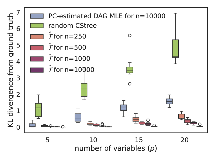
Figure 4: Evaluating accuracy of CStrees $\hat{\mathcal{T}}$ learned by Algorithm 1, compared to DAG models and random CStrees.

Since KL-divergence is a relative metric, we include two benchmark models. The first is a random CStree model whose KL-divergence from the ground truth data-generating model is computed and included in Figure 4 so as to give a sense of the accuracy of the models estimated by Algorithm 1 relative to the accuracy of random guessing.

The second benchmark is given by a DAG model. Since the constraint-based phase of our implementation of Algorithm 1 uses the PC algorithm, we take for this benchmark the estimated CPDAG computed in this phase. Hence, the difference in performance between the DAG model and the CStree model explicitly shows the performance of a model where additional steps are taken to include context-specific observations. If one chooses to use a different DAG learning algorithm in step 1 of Algorithm 1, one would analogously compare the CPDAG used in that step with the final output of Algorithm 1. For the DAG models, we compute only the KL-divergence for the model estimated from $n=10000$ samples, so as to give the best possible performing DAG in the comparisons.

Figure 4 shows that for all node sizes and all sample sizes, the accuracy of the CStree models is notably better than the accuracy of the DAG models. Indeed, even on 20 nodes where we are estimating a joint distribution with $2^{20}$ outcomes, the KL-divergence for the estimated CStrees is effectively zero ($n=10000)$, suggesting that Algorithm 1 is recovering the correct distribution with high probability.

In relation to other context-specific learning methods, we can focus in on the case of $p=10$ and $n=250$, where we see a median KL-divergence of approximately $0.2$. This may be compared with the experiments in [Hyttinen et al., 2018, Figure 3], where they use exact optimization techniques to estimate LDAGs on $p=10$ binary variables with a sample size of $n=200$. In the best case of their experiments they achieve a median KL-divergence of approximately $0.1$. This suggests that Algorithm 1 is quite competitive even with exact search methods that do not scale to large systems.

5.2 Scalability Evaluation

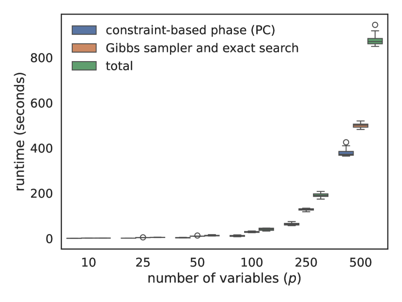
Figure 5: Runtimes for up to $p=500$ with $n=1000$.

To empirically evaluate scalability, we considered binary CStree models for $p\in\{10,20,50,100,250,500\}$ where the parents in a minimal DAG representation of the model are bounded by $\alpha=10$. This assumption is no stricter than standard practices when learning DAG models for large-scale systems. For $n=1000$, we generated $10$ such random CStrees for each $p$, and recorded the runtime in seconds for the constraint-based phase and the combined time for the MCMC and exact search phases for estimating the CStree. These runtimes are reported in Figure 5. We see the constraint-based phase accounts for approximately half of the total runtime for each $p$. The plot shows that even for $p=500$ variables, Algorithm 1 has a median runtime of only $15$ minutes. When considering also the observed accuracy of the method shown in Figure 4, this runtime is quite good compared to previous methods with high accuracy, such as the exact search methods of Hyttinen et al. [2018] where runtimes are on the order of hours, even for $p<50$.

5.3 Real World Example

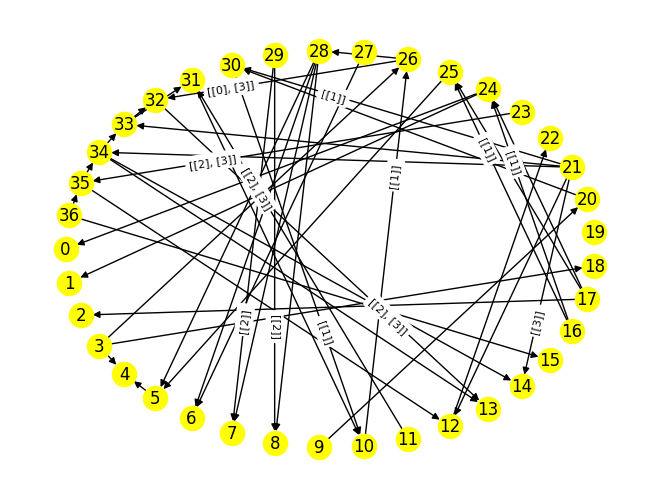
Figure 6: LDAG of the CStree learned for the ALARM data.

As a benchmark example for potential real data applications, we ran Algorithm 1 on the ALARM data set available in the bnlearn package in R. The data set consists of $20000$ joint samples from $37$ categorical variables including binary, ternary and quartic variables (see Appendix). The LDAG representation of the learned model is presented in Figure 6. With $41$ edges, the underlying DAG is slightly sparser than the benchmark DAG model, which has $46$ edges. The estimated CStree model captures $16$ CSI relations that cannot be captured by a DAG model of the data. These CSI relations are encoded in the $12$ edge labels in Figure 6, which include for instance $\mathcal{L}(29\rightarrow 8)=\{2\}$ and $\mathcal{L}(11\rightarrow 31)=\{2,3\}$. We interpret the observed CSI relations in terms of the real variables in the appendix.

Algorithm 1 returned this model in $14.188$ seconds. Hyttinen et al. [2018] used exact optimization to estimate an LDAG representation for the same data set, which took approximately $7$ hours. Since the benchmark DAG has nodes with parent sets bounded by only $4$, future work could aim to generalize Theorem 1 to $\beta=4$, allowing us to learn denser CStree models for the data set with likely only a marginal increase in time over the current $14.188$ seconds.

We included this example since it offers a nice comparison with the results of Hyttinen et al. [2018] for the same data set. A real data example is given in the appendix, where we apply Algorithm 1 to the well-known Sachs protein expression data set [Sachs et al., 2005]. The results for the Sachs data set also demonstrate how Algorithm 1, CStrees and their LDAG representations can efficiently discover and represent CSI relations in the data that are obscured by a DAG.

6 Future Work

The algorithm presented in this paper offers an accurate and scalable method for estimating sparse context-specific causal structures in the form of CStrees, which can be represented in multiple ways, including as an LDAG. The method relies on our ability to enumerate the models to be estimated, which is directly tied to the specific definition of a CStree, and consequently to a recently posed enumeration problem in combinatorics Alon and Balogh [2023]. To implement Algorithm 1, we solved this problem in the special case corresponding to CStrees in which all stages have at most $\beta=2$ context-defining variables (Theorem 1). To generalize Algorithm 1 to denser models, one could solve additional cases of this problem; e.g., $\beta=3,4,\ldots$. Since increasing $\beta$ increases the runtime of Algorithm 1, it is not necessary to solve this problem for arbitrary $\beta$, but only for reasonably small values, which seems within reach. Other interesting directions for future work include extending Algorithm 1 to support learning interventional CStree models as described in [Duarte and Solus, 2021], or to general stage trees where one need not solve as challenging of a combinatorial problem to achieve model enumeration. We note, however, that in this latter regime, we would lose the LDAG representation of the estimated models.

Scalable Structure Learning for Sparse Context-Specific Causal Systems
(Supplementary Material)

Appendix A Recovering the different graphical representations of a CStree

Recall from Section 3 that a CStree for categorical variables $(X_{1},\ldots,X_{p})$ is an ordered pair $\mathcal{T}=(\pi,\mathbf{s})$ where $\pi$ is a variable ordering and $\mathbf{s}$ is a collection of sets called the stages. The easiest representation to produce from directly from the pair $(\pi,\mathbf{s})$ is the staged tree representation, whose construction is detailed in Section 3. While the staged tree representation is perhaps the most direct graphical representation of the pair $(\pi,\mathbf{s})$, they are typically large graphs with numerous colored nodes that can make them difficult to directly interpret or manipulate. More interpretable representations include the LDAG representation of Pensar et al. [2015] and the minimal context graph representation of Duarte and Solus [2021]. The construction of these two representations from the pair $(\pi,\mathbf{s})$ is described below. Both make use of the so-called context-specific conditional independence axiom presented in [Corander et al., 2019] and [Duarte and Solus, 2021]:

• (Symmetry) If ${\bf X}_{A}\mathchoice{\mathrel{\hbox to0.0pt{$\displaystyle\perp$\hss}\mkern 2.0mu{\displaystyle\perp}}}{\mathrel{\hbox to0.0pt{$\textstyle\perp$\hss}\mkern 2.0mu{\textstyle\perp}}}{\mathrel{\hbox to0.0pt{$\scriptstyle\perp$\hss}\mkern 2.0mu{\scriptstyle\perp}}}{\mathrel{\hbox to0.0pt{$\scriptscriptstyle\perp$\hss}\mkern 2.0mu{\scriptscriptstyle\perp}}}{\bf X}_{B}|{\bf X}_{C},{\bf X}_{S}={\bf x}_{S}$ then ${\bf X}_{B}\mathchoice{\mathrel{\hbox to0.0pt{$\displaystyle\perp$\hss}\mkern 2.0mu{\displaystyle\perp}}}{\mathrel{\hbox to0.0pt{$\textstyle\perp$\hss}\mkern 2.0mu{\textstyle\perp}}}{\mathrel{\hbox to0.0pt{$\scriptstyle\perp$\hss}\mkern 2.0mu{\scriptstyle\perp}}}{\mathrel{\hbox to0.0pt{$\scriptscriptstyle\perp$\hss}\mkern 2.0mu{\scriptscriptstyle\perp}}}{\bf X}_{A}|{\bf X}_{C},{\bf X}_{S}={\bf x}_{S}$.

• (Decomposition) If ${\bf X}_{A}\mathchoice{\mathrel{\hbox to0.0pt{$\displaystyle\perp$\hss}\mkern 2.0mu{\displaystyle\perp}}}{\mathrel{\hbox to0.0pt{$\textstyle\perp$\hss}\mkern 2.0mu{\textstyle\perp}}}{\mathrel{\hbox to0.0pt{$\scriptstyle\perp$\hss}\mkern 2.0mu{\scriptstyle\perp}}}{\mathrel{\hbox to0.0pt{$\scriptscriptstyle\perp$\hss}\mkern 2.0mu{\scriptscriptstyle\perp}}}{\bf X}_{B\cup D}|{\bf X}_{C},{\bf X}_{S}={\bf x}_{S}$ then ${\bf X}_{A}\mathchoice{\mathrel{\hbox to0.0pt{$\displaystyle\perp$\hss}\mkern 2.0mu{\displaystyle\perp}}}{\mathrel{\hbox to0.0pt{$\textstyle\perp$\hss}\mkern 2.0mu{\textstyle\perp}}}{\mathrel{\hbox to0.0pt{$\scriptstyle\perp$\hss}\mkern 2.0mu{\scriptstyle\perp}}}{\mathrel{\hbox to0.0pt{$\scriptscriptstyle\perp$\hss}\mkern 2.0mu{\scriptscriptstyle\perp}}}{\bf X}_{B}|{\bf X}_{C},{\bf X}_{S}={\bf x}_{S}$.

• (Weak Union) If ${\bf X}_{A}\mathchoice{\mathrel{\hbox to0.0pt{$\displaystyle\perp$\hss}\mkern 2.0mu{\displaystyle\perp}}}{\mathrel{\hbox to0.0pt{$\textstyle\perp$\hss}\mkern 2.0mu{\textstyle\perp}}}{\mathrel{\hbox to0.0pt{$\scriptstyle\perp$\hss}\mkern 2.0mu{\scriptstyle\perp}}}{\mathrel{\hbox to0.0pt{$\scriptscriptstyle\perp$\hss}\mkern 2.0mu{\scriptscriptstyle\perp}}}{\bf X}_{B\cup D}|{\bf X}_{C},{\bf X}_{S}={\bf x}_{S}$ then ${\bf X}_{A}\mathchoice{\mathrel{\hbox to0.0pt{$\displaystyle\perp$\hss}\mkern 2.0mu{\displaystyle\perp}}}{\mathrel{\hbox to0.0pt{$\textstyle\perp$\hss}\mkern 2.0mu{\textstyle\perp}}}{\mathrel{\hbox to0.0pt{$\scriptstyle\perp$\hss}\mkern 2.0mu{\scriptstyle\perp}}}{\mathrel{\hbox to0.0pt{$\scriptscriptstyle\perp$\hss}\mkern 2.0mu{\scriptscriptstyle\perp}}}{\bf X}_{B}|{\bf X}_{C\cup D},{\bf X}_{S}={\bf x}_{S}$.

• (Contraction) If ${\bf X}_{A}\mathchoice{\mathrel{\hbox to0.0pt{$\displaystyle\perp$\hss}\mkern 2.0mu{\displaystyle\perp}}}{\mathrel{\hbox to0.0pt{$\textstyle\perp$\hss}\mkern 2.0mu{\textstyle\perp}}}{\mathrel{\hbox to0.0pt{$\scriptstyle\perp$\hss}\mkern 2.0mu{\scriptstyle\perp}}}{\mathrel{\hbox to0.0pt{$\scriptscriptstyle\perp$\hss}\mkern 2.0mu{\scriptscriptstyle\perp}}}{\bf X}_{B}|{\bf X}_{C\cup D},{\bf X}_{S}={\bf x}_{S}$ and ${\bf X}_{A}\mathchoice{\mathrel{\hbox to0.0pt{$\displaystyle\perp$\hss}\mkern 2.0mu{\displaystyle\perp}}}{\mathrel{\hbox to0.0pt{$\textstyle\perp$\hss}\mkern 2.0mu{\textstyle\perp}}}{\mathrel{\hbox to0.0pt{$\scriptstyle\perp$\hss}\mkern 2.0mu{\scriptstyle\perp}}}{\mathrel{\hbox to0.0pt{$\scriptscriptstyle\perp$\hss}\mkern 2.0mu{\scriptscriptstyle\perp}}}{\bf X}_{D}|{\bf X}_{C},{\bf X}_{S}={\bf x}_{S}$ then ${\bf X}_{A}\mathchoice{\mathrel{\hbox to0.0pt{$\displaystyle\perp$\hss}\mkern 2.0mu{\displaystyle\perp}}}{\mathrel{\hbox to0.0pt{$\textstyle\perp$\hss}\mkern 2.0mu{\textstyle\perp}}}{\mathrel{\hbox to0.0pt{$\scriptstyle\perp$\hss}\mkern 2.0mu{\scriptstyle\perp}}}{\mathrel{\hbox to0.0pt{$\scriptscriptstyle\perp$\hss}\mkern 2.0mu{\scriptscriptstyle\perp}}}{\bf X}_{B\cup D}|{\bf X}_{C},{\bf X}_{S}={\bf x}_{S}$

• (Intersection) If ${\bf X}_{A}\mathchoice{\mathrel{\hbox to0.0pt{$\displaystyle\perp$\hss}\mkern 2.0mu{\displaystyle\perp}}}{\mathrel{\hbox to0.0pt{$\textstyle\perp$\hss}\mkern 2.0mu{\textstyle\perp}}}{\mathrel{\hbox to0.0pt{$\scriptstyle\perp$\hss}\mkern 2.0mu{\scriptstyle\perp}}}{\mathrel{\hbox to0.0pt{$\scriptscriptstyle\perp$\hss}\mkern 2.0mu{\scriptscriptstyle\perp}}}{\bf X}_{B}|{\bf X}_{C\cup D},{\bf X}_{S}={\bf x}_{S}$ and ${\bf X}_{A}\mathchoice{\mathrel{\hbox to0.0pt{$\displaystyle\perp$\hss}\mkern 2.0mu{\displaystyle\perp}}}{\mathrel{\hbox to0.0pt{$\textstyle\perp$\hss}\mkern 2.0mu{\textstyle\perp}}}{\mathrel{\hbox to0.0pt{$\scriptstyle\perp$\hss}\mkern 2.0mu{\scriptstyle\perp}}}{\mathrel{\hbox to0.0pt{$\scriptscriptstyle\perp$\hss}\mkern 2.0mu{\scriptscriptstyle\perp}}}{\bf X}_{D}|{\bf X}_{C\cup B},{\bf X}_{S}={\bf x}_{S}$ then ${\bf X}_{A}\mathchoice{\mathrel{\hbox to0.0pt{$\displaystyle\perp$\hss}\mkern 2.0mu{\displaystyle\perp}}}{\mathrel{\hbox to0.0pt{$\textstyle\perp$\hss}\mkern 2.0mu{\textstyle\perp}}}{\mathrel{\hbox to0.0pt{$\scriptstyle\perp$\hss}\mkern 2.0mu{\scriptstyle\perp}}}{\mathrel{\hbox to0.0pt{$\scriptscriptstyle\perp$\hss}\mkern 2.0mu{\scriptscriptstyle\perp}}}{\bf X}_{B\cup D}|{\bf X}_{C},{\bf X}_{S}={\bf x}_{S}$.

• (Specialization) If ${\bf X}_{A}\mathchoice{\mathrel{\hbox to0.0pt{$\displaystyle\perp$\hss}\mkern 2.0mu{\displaystyle\perp}}}{\mathrel{\hbox to0.0pt{$\textstyle\perp$\hss}\mkern 2.0mu{\textstyle\perp}}}{\mathrel{\hbox to0.0pt{$\scriptstyle\perp$\hss}\mkern 2.0mu{\scriptstyle\perp}}}{\mathrel{\hbox to0.0pt{$\scriptscriptstyle\perp$\hss}\mkern 2.0mu{\scriptscriptstyle\perp}}}{\bf X}_{B}|{\bf X}_{C},{\bf X}_{S}={\bf x}_{S}$ and $D\subseteq C$ then ${\bf X}_{A}\mathchoice{\mathrel{\hbox to0.0pt{$\displaystyle\perp$\hss}\mkern 2.0mu{\displaystyle\perp}}}{\mathrel{\hbox to0.0pt{$\textstyle\perp$\hss}\mkern 2.0mu{\textstyle\perp}}}{\mathrel{\hbox to0.0pt{$\scriptstyle\perp$\hss}\mkern 2.0mu{\scriptstyle\perp}}}{\mathrel{\hbox to0.0pt{$\scriptscriptstyle\perp$\hss}\mkern 2.0mu{\scriptscriptstyle\perp}}}{\bf X}_{B}|{\bf X}_{C\setminus D},{\bf X}_{S\cup D}={\bf x}_{S}{\bf x}_{D}$ for all ${\bf x}_{D}\in\mathcal{X}_{D}$.

• (Absorption) If ${\bf X}_{A}\mathchoice{\mathrel{\hbox to0.0pt{$\displaystyle\perp$\hss}\mkern 2.0mu{\displaystyle\perp}}}{\mathrel{\hbox to0.0pt{$\textstyle\perp$\hss}\mkern 2.0mu{\textstyle\perp}}}{\mathrel{\hbox to0.0pt{$\scriptstyle\perp$\hss}\mkern 2.0mu{\scriptstyle\perp}}}{\mathrel{\hbox to0.0pt{$\scriptscriptstyle\perp$\hss}\mkern 2.0mu{\scriptscriptstyle\perp}}}{\bf X}_{B}|{\bf X}_{C},{\bf X}_{S}={\bf x}_{S}$ and $D\subseteq S$ such that ${\bf X}_{A}\mathchoice{\mathrel{\hbox to0.0pt{$\displaystyle\perp$\hss}\mkern 2.0mu{\displaystyle\perp}}}{\mathrel{\hbox to0.0pt{$\textstyle\perp$\hss}\mkern 2.0mu{\textstyle\perp}}}{\mathrel{\hbox to0.0pt{$\scriptstyle\perp$\hss}\mkern 2.0mu{\scriptstyle\perp}}}{\mathrel{\hbox to0.0pt{$\scriptscriptstyle\perp$\hss}\mkern 2.0mu{\scriptscriptstyle\perp}}}{\bf X}_{B}|{\bf X}_{C},{\bf X}_{S}={\bf x}_{S\setminus D}{\bf y}_{D}$ for all ${\bf y}_{D}\in\mathcal{X}_{D}$ then ${\bf X}_{A}\mathchoice{\mathrel{\hbox to0.0pt{$\displaystyle\perp$\hss}\mkern 2.0mu{\displaystyle\perp}}}{\mathrel{\hbox to0.0pt{$\textstyle\perp$\hss}\mkern 2.0mu{\textstyle\perp}}}{\mathrel{\hbox to0.0pt{$\scriptstyle\perp$\hss}\mkern 2.0mu{\scriptstyle\perp}}}{\mathrel{\hbox to0.0pt{$\scriptscriptstyle\perp$\hss}\mkern 2.0mu{\scriptscriptstyle\perp}}}{\bf X}_{B}|{\bf X}_{C\cup D},{\bf X}_{S\setminus D}={\bf x}_{S\setminus D}$.

The above implications hold for all positive probability distributions.

A.1 The LDAG representation

Given a CStree $\mathcal{T}=(\pi,\mathbf{s})$ the set of stages is a disjoint union $\mathbf{s}=\mathbf{s}_{i}\cup\cdots\cup\mathbf{s}_{p}$ where

$$\mathbf{s}_{i}=\{\mathcal{S}_{\pi,i}({\bf x}_{S}):X_{\pi_{i}}\mathchoice{\mathrel{\hbox to0.0pt{$\displaystyle\perp$\hss}\mkern 2.0mu{\displaystyle\perp}}}{\mathrel{\hbox to0.0pt{$\textstyle\perp$\hss}\mkern 2.0mu{\textstyle\perp}}}{\mathrel{\hbox to0.0pt{$\scriptstyle\perp$\hss}\mkern 2.0mu{\scriptstyle\perp}}}{\mathrel{\hbox to0.0pt{$\scriptscriptstyle\perp$\hss}\mkern 2.0mu{\scriptscriptstyle\perp}}}{\bf X}_{[\pi_{1}:\pi_{i-1}]\setminus S}|{\bf X}_{S}={\bf x}_{S}\in\mathcal{C}_{\pi,i}\}.$$

Each set $\mathcal{S}_{\pi,i}({\bf x}_{S})$ consists of all joint outcomes ${\bf x}_{[\pi_{1}:\pi_{i-1}]}\in\mathcal{X}_{[\pi_{1}:\pi_{i-1}]}$ that agree with the context ${\bf x}_{S}$ when restricted to the values $x_{i}$ for $i\in S$. Hence, from the elements of the set $\mathcal{S}_{\pi,i}({\bf x}_{S})$ we can directly deduce the context ${\bf X}_{S}={\bf x}_{S}$ and recover the CSI relation

$$X_{\pi_{i}}\mathchoice{\mathrel{\hbox to0.0pt{$\displaystyle\perp$\hss}\mkern 2.0mu{\displaystyle\perp}}}{\mathrel{\hbox to0.0pt{$\textstyle\perp$\hss}\mkern 2.0mu{\textstyle\perp}}}{\mathrel{\hbox to0.0pt{$\scriptstyle\perp$\hss}\mkern 2.0mu{\scriptstyle\perp}}}{\mathrel{\hbox to0.0pt{$\scriptscriptstyle\perp$\hss}\mkern 2.0mu{\scriptscriptstyle\perp}}}{\bf X}_{[\pi_{1}:\pi_{i-1}]\setminus S}|{\bf X}_{S}={\bf x}_{S}.$$

Doing this for all $\mathcal{S}_{\pi,i}({\bf x}_{S})\in\mathbf{s}_{i}$ produces the set of CSI relations

$$\mathcal{C}_{\pi,i}=\{X_{\pi_{i}}\mathchoice{\mathrel{\hbox to0.0pt{$\displaystyle\perp$\hss}\mkern 2.0mu{\displaystyle\perp}}}{\mathrel{\hbox to0.0pt{$\textstyle\perp$\hss}\mkern 2.0mu{\textstyle\perp}}}{\mathrel{\hbox to0.0pt{$\scriptstyle\perp$\hss}\mkern 2.0mu{\scriptstyle\perp}}}{\mathrel{\hbox to0.0pt{$\scriptscriptstyle\perp$\hss}\mkern 2.0mu{\scriptscriptstyle\perp}}}{\bf X}_{[\pi_{1}:\pi_{i-1}]\setminus S}|{\bf X}_{S}={\bf x}_{S}\mbox{ entailed by ${\bf X}$}\}.$$

Taking the union over the sets $S\subset[\pi_{1}:\pi_{i-1}]$ for which there is a relation in $\mathcal{C}_{\pi,i}$ with context ${\bf X}_{S}={\bf x}_{S}$ we obtain a set $\Pi(\pi_{i})$. Recall that it is also possible that $W(i):=\mathcal{X}_{\pi_{1}:\pi_{i-1}]}\setminus\bigcup_{s\in\mathbf{s}_{i}}s\neq\emptyset$. (The elements in this set are in bijection with the white nodes at level $i$ in the rooted tree $\mathcal{T}$.) If $W_{i}\neq\emptyset$ then there exist outcomes $X_{\pi_{i}}$ that possible depend on all variables $X_{\pi_{1}},\ldots,X_{\pi_{i-1}}$. Hence, if $W_{i}\neq\emptyset$ we set $\operatorname{pa}_{\operatorname{\mathcal{G}}}(\pi_{i}):=\{\pi_{1},\ldots,\pi_{i-1}\}$. Otherwise, we set $\operatorname{pa}_{\operatorname{\mathcal{G}}}(\pi_{i}):=Pi(\pi_{i})$ It follows that the set $\operatorname{pa}_{\operatorname{\mathcal{G}}}(\pi_{i})$ are the parents of node $i$ in a DAG $\operatorname{\mathcal{G}}=([p],E)$ to which the distribution ${\bf X}$ is Markov. This DAG is called a (minimal) I-MAP of the CStree $\mathcal{T}$.

Example 1.

Consider the CStree from the example in Section 3 defined by the collection of CSI relations

$$\begin{split}\mathcal{C}_{\mathcal{T}}=\{&X_{2}\mathchoice{\mathrel{\hbox to0.0pt{$\displaystyle\perp$\hss}\mkern 2.0mu{\displaystyle\perp}}}{\mathrel{\hbox to0.0pt{$\textstyle\perp$\hss}\mkern 2.0mu{\textstyle\perp}}}{\mathrel{\hbox to0.0pt{$\scriptstyle\perp$\hss}\mkern 2.0mu{\scriptstyle\perp}}}{\mathrel{\hbox to0.0pt{$\scriptscriptstyle\perp$\hss}\mkern 2.0mu{\scriptscriptstyle\perp}}}X_{1},\\ &X_{3}\mathchoice{\mathrel{\hbox to0.0pt{$\displaystyle\perp$\hss}\mkern 2.0mu{\displaystyle\perp}}}{\mathrel{\hbox to0.0pt{$\textstyle\perp$\hss}\mkern 2.0mu{\textstyle\perp}}}{\mathrel{\hbox to0.0pt{$\scriptstyle\perp$\hss}\mkern 2.0mu{\scriptstyle\perp}}}{\mathrel{\hbox to0.0pt{$\scriptscriptstyle\perp$\hss}\mkern 2.0mu{\scriptscriptstyle\perp}}}X_{1}|X_{2}=1,\\ &X_{4}\mathchoice{\mathrel{\hbox to0.0pt{$\displaystyle\perp$\hss}\mkern 2.0mu{\displaystyle\perp}}}{\mathrel{\hbox to0.0pt{$\textstyle\perp$\hss}\mkern 2.0mu{\textstyle\perp}}}{\mathrel{\hbox to0.0pt{$\scriptstyle\perp$\hss}\mkern 2.0mu{\scriptstyle\perp}}}{\mathrel{\hbox to0.0pt{$\scriptscriptstyle\perp$\hss}\mkern 2.0mu{\scriptscriptstyle\perp}}}X_{2}|X_{1,3}=(1,1),\\ &X_{4}\mathchoice{\mathrel{\hbox to0.0pt{$\displaystyle\perp$\hss}\mkern 2.0mu{\displaystyle\perp}}}{\mathrel{\hbox to0.0pt{$\textstyle\perp$\hss}\mkern 2.0mu{\textstyle\perp}}}{\mathrel{\hbox to0.0pt{$\scriptstyle\perp$\hss}\mkern 2.0mu{\scriptstyle\perp}}}{\mathrel{\hbox to0.0pt{$\scriptscriptstyle\perp$\hss}\mkern 2.0mu{\scriptscriptstyle\perp}}}X_{2}|X_{1,3}=(1,0),\\ &X_{4}\mathchoice{\mathrel{\hbox to0.0pt{$\displaystyle\perp$\hss}\mkern 2.0mu{\displaystyle\perp}}}{\mathrel{\hbox to0.0pt{$\textstyle\perp$\hss}\mkern 2.0mu{\textstyle\perp}}}{\mathrel{\hbox to0.0pt{$\scriptstyle\perp$\hss}\mkern 2.0mu{\scriptstyle\perp}}}{\mathrel{\hbox to0.0pt{$\scriptscriptstyle\perp$\hss}\mkern 2.0mu{\scriptscriptstyle\perp}}}X_{2}|X_{1,3}=(0,1)\}.\end{split}$$

To recover the minimal I-MAP $\operatorname{\mathcal{G}}$ for $\mathcal{T}$, we start with the node $4$. There are exactly three CSI relations for the variable $X_{4}$:

$$X_{4}\mathchoice{\mathrel{\hbox to0.0pt{$\displaystyle\perp$\hss}\mkern 2.0mu{\displaystyle\perp}}}{\mathrel{\hbox to0.0pt{$\textstyle\perp$\hss}\mkern 2.0mu{\textstyle\perp}}}{\mathrel{\hbox to0.0pt{$\scriptstyle\perp$\hss}\mkern 2.0mu{\scriptstyle\perp}}}{\mathrel{\hbox to0.0pt{$\scriptscriptstyle\perp$\hss}\mkern 2.0mu{\scriptscriptstyle\perp}}}X_{2}|X_{1,3}=(1,1),\qquad X_{4}\mathchoice{\mathrel{\hbox to0.0pt{$\displaystyle\perp$\hss}\mkern 2.0mu{\displaystyle\perp}}}{\mathrel{\hbox to0.0pt{$\textstyle\perp$\hss}\mkern 2.0mu{\textstyle\perp}}}{\mathrel{\hbox to0.0pt{$\scriptstyle\perp$\hss}\mkern 2.0mu{\scriptstyle\perp}}}{\mathrel{\hbox to0.0pt{$\scriptscriptstyle\perp$\hss}\mkern 2.0mu{\scriptscriptstyle\perp}}}X_{2}|X_{1,3}=(1,0)\qquad\mbox{and}\qquad X_{4}\mathchoice{\mathrel{\hbox to0.0pt{$\displaystyle\perp$\hss}\mkern 2.0mu{\displaystyle\perp}}}{\mathrel{\hbox to0.0pt{$\textstyle\perp$\hss}\mkern 2.0mu{\textstyle\perp}}}{\mathrel{\hbox to0.0pt{$\scriptstyle\perp$\hss}\mkern 2.0mu{\scriptstyle\perp}}}{\mathrel{\hbox to0.0pt{$\scriptscriptstyle\perp$\hss}\mkern 2.0mu{\scriptscriptstyle\perp}}}X_{2}|X_{1,3}=(0,1),$$

and each of these relations has contexts given by the variables $\{X_{1},X_{3}\}$. Hence, $\Pi(4)=\{1,3\}$. However, there exist white nodes in the fourth level of the tree $\mathcal{T}$, indicating that the set $W(4)\neq\emptyset$. In particular, $W(4)=\{(0,0,0),(0,1,0)\}$. Hence, the parents of $4$ in $\operatorname{\mathcal{G}}$ are $\operatorname{pa}_{\operatorname{\mathcal{G}}}(4)=\{1,2,3\}$. Similarly, the parents of $3$ in $\operatorname{\mathcal{G}}$ are $\operatorname{pa}_{\operatorname{\mathcal{G}}}(3)=\{1,2\}$.

Finally, note that the relation $X_{2}\mathchoice{\mathrel{\hbox to0.0pt{$\displaystyle\perp$\hss}\mkern 2.0mu{\displaystyle\perp}}}{\mathrel{\hbox to0.0pt{$\textstyle\perp$\hss}\mkern 2.0mu{\textstyle\perp}}}{\mathrel{\hbox to0.0pt{$\scriptstyle\perp$\hss}\mkern 2.0mu{\scriptstyle\perp}}}{\mathrel{\hbox to0.0pt{$\scriptscriptstyle\perp$\hss}\mkern 2.0mu{\scriptscriptstyle\perp}}}X_{1}$ is a genuine CI relation, and therefore it is defined by the context ${\bf X}_{\emptyset}={\bf x}_{\emptyset}$. Hence, the parent set of node $2$ in $\operatorname{\mathcal{G}}$ is $\operatorname{pa}_{\operatorname{\mathcal{G}}}(2)=\emptyset$. (Note that in this case, the set $W(2)=\emptyset$.) Since there are no relations for node $1$, we further have that the parents of node $1$ in $\operatorname{\mathcal{G}}$ are $\operatorname{pa}_{\operatorname{\mathcal{G}}}(1)=\emptyset$. It follows that the minimal I-MAP of the CStree $\mathcal{T}$ is

which is the DAG from Figure 3 in Section 3. $\square$

The resulting DAG $\mathcal{G}$ is the DAG forming the basis for the LDAG representation. It remains to identify the edge labels. In an LDAG, the edges $j\rightarrow i\in E$ are labeled with a set of contexts ${\bf x}_{\operatorname{pa}_{\operatorname{\mathcal{G}}}(i)\setminus\{j\}}$ such that $X_{i}\mathchoice{\mathrel{\hbox to0.0pt{$\displaystyle\perp$\hss}\mkern 2.0mu{\displaystyle\perp}}}{\mathrel{\hbox to0.0pt{$\textstyle\perp$\hss}\mkern 2.0mu{\textstyle\perp}}}{\mathrel{\hbox to0.0pt{$\scriptstyle\perp$\hss}\mkern 2.0mu{\scriptstyle\perp}}}{\mathrel{\hbox to0.0pt{$\scriptscriptstyle\perp$\hss}\mkern 2.0mu{\scriptscriptstyle\perp}}}X_{j}|{\bf X}_{\operatorname{pa}_{\operatorname{\mathcal{G}}}(i)\setminus\{j\}}={\bf x}_{\operatorname{pa}_{\operatorname{\mathcal{G}}}(i)\setminus\{j\}}$. For the minimal I-MAP $\operatorname{\mathcal{G}}$ of $\mathcal{T}$, we know that for each $X_{\pi_{i}}\mathchoice{\mathrel{\hbox to0.0pt{$\displaystyle\perp$\hss}\mkern 2.0mu{\displaystyle\perp}}}{\mathrel{\hbox to0.0pt{$\textstyle\perp$\hss}\mkern 2.0mu{\textstyle\perp}}}{\mathrel{\hbox to0.0pt{$\scriptstyle\perp$\hss}\mkern 2.0mu{\scriptstyle\perp}}}{\mathrel{\hbox to0.0pt{$\scriptscriptstyle\perp$\hss}\mkern 2.0mu{\scriptscriptstyle\perp}}}{\bf X}_{[\pi_{1}:\pi_{i-1}]\setminus S}|{\bf X}_{S}={\bf x}_{S}\in\mathcal{C}_{\pi,i}$ the set $S$ is a subset of the set $\operatorname{pa}_{\operatorname{\mathcal{G}}}(\pi_{i})$. Applying the weak union property for CSI relations, we know that the distributions in the CStree model $\mathcal{M}(\mathcal{T})$ satisfy the relations

$$X_{\pi_{i}}\mathchoice{\mathrel{\hbox to0.0pt{$\displaystyle\perp$\hss}\mkern 2.0mu{\displaystyle\perp}}}{\mathrel{\hbox to0.0pt{$\textstyle\perp$\hss}\mkern 2.0mu{\textstyle\perp}}}{\mathrel{\hbox to0.0pt{$\scriptstyle\perp$\hss}\mkern 2.0mu{\scriptstyle\perp}}}{\mathrel{\hbox to0.0pt{$\scriptscriptstyle\perp$\hss}\mkern 2.0mu{\scriptscriptstyle\perp}}}{\bf X}_{[\pi_{1}:\pi_{i-1}]\setminus\operatorname{pa}_{\operatorname{\mathcal{G}}}(\pi_{i})}|{\bf X}_{\operatorname{pa}_{\operatorname{\mathcal{G}}}(\pi_{i})\setminus S},{\bf X}_{S}={\bf x}_{S}.$$

Applying the decomposition property it follows that the distributions in $\mathcal{M}(\mathcal{T})$ satisfy

$$X_{\pi_{i}}\mathchoice{\mathrel{\hbox to0.0pt{$\displaystyle\perp$\hss}\mkern 2.0mu{\displaystyle\perp}}}{\mathrel{\hbox to0.0pt{$\textstyle\perp$\hss}\mkern 2.0mu{\textstyle\perp}}}{\mathrel{\hbox to0.0pt{$\scriptstyle\perp$\hss}\mkern 2.0mu{\scriptstyle\perp}}}{\mathrel{\hbox to0.0pt{$\scriptscriptstyle\perp$\hss}\mkern 2.0mu{\scriptscriptstyle\perp}}}X_{j}|{\bf X}_{\operatorname{pa}_{\operatorname{\mathcal{G}}}(\pi_{i})\setminus S},{\bf X}_{S}={\bf x}_{S}$$

for all $j\in[\pi_{1}:\pi_{i-1}]\setminus\operatorname{pa}_{\operatorname{\mathcal{G}}}(i)$, for all contexts ${\bf X}_{S}={\bf x}_{S}$ defining the CSI relations in $\mathcal{C}_{\pi,i}$. Hence, the label for the edge $j\rightarrow\pi_{i}$ in $\operatorname{\mathcal{G}}$ would be the set

$$\mathcal{L}(j\rightarrow\pi_{i})=\{{\bf x}_{\operatorname{pa}_{\operatorname{\mathcal{G}}}(\pi_{i})\setminus S}{\bf x}_{S}:{\bf X}_{S}={\bf x}_{S}\mbox{ defines a relation in $\mathcal{C}_{\pi,i}$ and }{\bf x}_{\operatorname{pa}_{\operatorname{\mathcal{G}}}(\pi_{i})\setminus S}\in\mathcal{X}_{\operatorname{pa}_{\operatorname{\mathcal{G}}}(\pi_{i})\setminus S}\}.$$

The set $\mathcal{L}(j\rightarrow\pi_{i})$ can be very large. To simplify its representation it is typical to use a $\ast$ symbol in the coordinate for outcome $x_{k}$ to indicate that the context is in the set for all $x_{k}\in\mathcal{X}_{k}$.

Example 1 continued.

We first compute the edge label $\mathcal{L}(2\rightarrow 4)$ for the DAG $\operatorname{\mathcal{G}}$ in Example 1. Since we know that the CSI relations

$$X_{4}\mathchoice{\mathrel{\hbox to0.0pt{$\displaystyle\perp$\hss}\mkern 2.0mu{\displaystyle\perp}}}{\mathrel{\hbox to0.0pt{$\textstyle\perp$\hss}\mkern 2.0mu{\textstyle\perp}}}{\mathrel{\hbox to0.0pt{$\scriptstyle\perp$\hss}\mkern 2.0mu{\scriptstyle\perp}}}{\mathrel{\hbox to0.0pt{$\scriptscriptstyle\perp$\hss}\mkern 2.0mu{\scriptscriptstyle\perp}}}X_{2}|X_{1,3}=(1,1),\qquad X_{4}\mathchoice{\mathrel{\hbox to0.0pt{$\displaystyle\perp$\hss}\mkern 2.0mu{\displaystyle\perp}}}{\mathrel{\hbox to0.0pt{$\textstyle\perp$\hss}\mkern 2.0mu{\textstyle\perp}}}{\mathrel{\hbox to0.0pt{$\scriptstyle\perp$\hss}\mkern 2.0mu{\scriptstyle\perp}}}{\mathrel{\hbox to0.0pt{$\scriptscriptstyle\perp$\hss}\mkern 2.0mu{\scriptscriptstyle\perp}}}X_{2}|X_{1,3}=(1,0)\qquad\mbox{and}\qquad X_{4}\mathchoice{\mathrel{\hbox to0.0pt{$\displaystyle\perp$\hss}\mkern 2.0mu{\displaystyle\perp}}}{\mathrel{\hbox to0.0pt{$\textstyle\perp$\hss}\mkern 2.0mu{\textstyle\perp}}}{\mathrel{\hbox to0.0pt{$\scriptstyle\perp$\hss}\mkern 2.0mu{\scriptstyle\perp}}}{\mathrel{\hbox to0.0pt{$\scriptscriptstyle\perp$\hss}\mkern 2.0mu{\scriptscriptstyle\perp}}}X_{2}|X_{1,3}=(0,1),$$

hold, we obtain the edge label

$$\mathcal{L}(2\rightarrow 4)=\{(0,1),(1,0),(1,1)\}\subset\mathcal{X}_{\operatorname{pa}_{\operatorname{\mathcal{G}}}(4)\setminus\{2\}}.$$

Since $(0,1)$ and $(1,1)$ are both in $\mathcal{L}(2\rightarrow 4)$ we can represent this pair of outcomes more simply as $(\ast,1)$. Similarly, the pair $(1,0)$ and $(1,1)$ can be represented as $(1,\ast)$. (Note that this representation redundantly represents the single outcome $(1,1)$, but it results in a simpler edge label:

$$\mathcal{L}(2\rightarrow 4)=\{(1,\ast),(\ast,1)\}.$$

This is the edge label of the edge $2\rightarrow 4$ in the LDAG in Figure 2. The remaining edge labels can be calculated analogously, yielding the LDAG representation of the CStree $\mathcal{T}$:

Note that if an edge label $\mathcal{L}(j\rightarrow i)$ is the emptyset, we simply do not draw it. This indicate that the dependency represented by this edge vansishes under no contexts.

Remark 1.

Note that the LDAG above is a representation of the pairwise CSI relations $X_{i}\mathchoice{\mathrel{\hbox to0.0pt{$\displaystyle\perp$\hss}\mkern 2.0mu{\displaystyle\perp}}}{\mathrel{\hbox to0.0pt{$\textstyle\perp$\hss}\mkern 2.0mu{\textstyle\perp}}}{\mathrel{\hbox to0.0pt{$\scriptstyle\perp$\hss}\mkern 2.0mu{\scriptstyle\perp}}}{\mathrel{\hbox to0.0pt{$\scriptscriptstyle\perp$\hss}\mkern 2.0mu{\scriptscriptstyle\perp}}}X_{j}|{\bf X}_{\operatorname{pa}_{\operatorname{\mathcal{G}}}(i)\setminus j}={\bf x}_{\operatorname{pa}_{\operatorname{\mathcal{G}}}(i)\setminus j}$ that hold in the distribution. However, arbitrary discrete distributions do not satisfy the composition axiom:

• (Composition) If ${\bf X}_{A}\mathchoice{\mathrel{\hbox to0.0pt{$\displaystyle\perp$\hss}\mkern 2.0mu{\displaystyle\perp}}}{\mathrel{\hbox to0.0pt{$\textstyle\perp$\hss}\mkern 2.0mu{\textstyle\perp}}}{\mathrel{\hbox to0.0pt{$\scriptstyle\perp$\hss}\mkern 2.0mu{\scriptstyle\perp}}}{\mathrel{\hbox to0.0pt{$\scriptscriptstyle\perp$\hss}\mkern 2.0mu{\scriptscriptstyle\perp}}}{\bf X}_{B}|{\bf x}_{C},{\bf X}_{S}={\bf x}_{S}$ and ${\bf X}_{A}\mathchoice{\mathrel{\hbox to0.0pt{$\displaystyle\perp$\hss}\mkern 2.0mu{\displaystyle\perp}}}{\mathrel{\hbox to0.0pt{$\textstyle\perp$\hss}\mkern 2.0mu{\textstyle\perp}}}{\mathrel{\hbox to0.0pt{$\scriptstyle\perp$\hss}\mkern 2.0mu{\scriptstyle\perp}}}{\mathrel{\hbox to0.0pt{$\scriptscriptstyle\perp$\hss}\mkern 2.0mu{\scriptscriptstyle\perp}}}{\bf X}_{D}|{\bf X}_{C},{\bf X}_{S}={\bf x}_{S}$ then ${\bf X}_{A}\mathchoice{\mathrel{\hbox to0.0pt{$\displaystyle\perp$\hss}\mkern 2.0mu{\displaystyle\perp}}}{\mathrel{\hbox to0.0pt{$\textstyle\perp$\hss}\mkern 2.0mu{\textstyle\perp}}}{\mathrel{\hbox to0.0pt{$\scriptstyle\perp$\hss}\mkern 2.0mu{\scriptstyle\perp}}}{\mathrel{\hbox to0.0pt{$\scriptscriptstyle\perp$\hss}\mkern 2.0mu{\scriptscriptstyle\perp}}}{\bf x}_{B\cup D}|{\bf X}_{C},{\bf X}_{S}={\bf x}_{S}$.

To construct the LDAG representation of a CStree we used the decomposition axiom to produce the pairwise relations holding in the CStree model that are used to construct the LDAG. However, it is possible that a distribution satisfies these pairwise CSI relations but not the defining CSI relations of the CStree. Consequently, while one can represent a CStree model with an LDAG, one cannot necessarily learn an LDAG directly (via the structure learning equations in [Hyttinen et al., 2018, Pensar et al., 2015] and deduce that the distribution belongs to the CStree model. This is because the data-generating distribution Markov to the learned LDAG representation may not satisfy composition, meaning that one cannot directly conclude that the distribution is Markov to the corresponding CStree without verifying that additional CSI relations hold. Specifically, the CStree model provides stronger CSI relations than those one can deduce from the LDAG unless one can show that distributions in these models satisfy composition. Since our algorithm learns a CStree model according to the staged tree representation, we can however, use an LDAG representation of the model for compactness while keeping in mind that the model fulfills the additional CSI relations used in the factorization (3).

A.2 The Minimal Context Graph Representation

An alternative to the LDAG representation of a CStree is the representation of the model via a collection of DAGs, one for each element of a set of minimal contexts. A minimal context is defined in the following way: Let $\mathcal{J}(\mathcal{T})$ denote the complete set of CSI relations that are implied by those defining the model $\mathcal{M}(\mathcal{T})$ via repeated application of the context-specific conditional independence axioms above. Let ${\bf X}_{A}\mathchoice{\mathrel{\hbox to0.0pt{$\displaystyle\perp$\hss}\mkern 2.0mu{\displaystyle\perp}}}{\mathrel{\hbox to0.0pt{$\textstyle\perp$\hss}\mkern 2.0mu{\textstyle\perp}}}{\mathrel{\hbox to0.0pt{$\scriptstyle\perp$\hss}\mkern 2.0mu{\scriptstyle\perp}}}{\mathrel{\hbox to0.0pt{$\scriptscriptstyle\perp$\hss}\mkern 2.0mu{\scriptscriptstyle\perp}}}{\bf X}_{B}|{\bf X}_{C},{\bf X}_{D}={\bf x}_{D}$ be any relation in $\mathcal{J}(\mathcal{T})$. We may apply the absorption axiom to this relation until the cardinality of the variables $D$ defining the context can no longer be reduced. The contexts obtained by doing this for all possible elements of $\mathcal{J}(\mathcal{T})$ in all possible ways of applying absorption is necessarily a finite set of contexts, called the minimal contexts. For each such context, ${\bf X}_{D}={\bf x}_{D}$, we can consider the I-MAP of the CSI relations with this context that live in $\mathcal{J}(\mathcal{T})$. This is a DAG whose d-separations encode the CSI relations with context ${\bf X}_{D}={\bf x}_{D}$. For example, the minimal context graph representation of the CStree depicted in Figure 1 is

It is shown in [Duarte and Solus, 2021] that two CStrees define the same set of distributions (i.e. are Markov equivalent) if and only if they have the same set of minimal contexts and each context gives a pair of Markov equivalent DAGs. This makes this representation useful for deducing model equivalence. However, it is currently an intractable representation to compute for large systems of variables. Hence, we use the LDAG representation throughout this paper.

Appendix B Enumerating the Possible Stagings for Sparse CStrees

In this section, we describe a method for producing a list of all possible CStrees $\mathcal{T}=(\pi,\mathbf{s})$ with stages defined by contexts ${\bf x}_{S}$ with $|S|\leq 2$ for distributions $(X_{1},\ldots,X_{p})$ with state space $\mathcal{X}=\prod_{i=1}^{p}[d_{i}]$ and $d_{1},\ldots,d_{p}>1$. This is a necessary computation for computing the local and order scores in (7) and  (5) that are used in both the stochastic search and exact optimization phases of the algorithm. Since the variable ordering is fixed, we assume in the following that it is the natural ordering $\pi=12\cdots p$ and build a list of possible stagings for each level $\mathcal{X}_{[i]}$. Each staging corresponds to a way to color the nodes $\mathcal{X}_{[i]}$ in the staged tree representation of the CStree given in Figure 1. In the following, we refer to the set of nodes $\mathcal{X}_{[i]}$ as level $i$ of the CStree. Identifying all colorings of level $i$ that yield a CStree in turn yields a way to construct all CStrees since any one stage only contains vertices of the tree in a single level.

Recall that a stage $\mathcal{S}({\bf x}_{S})\subset\mathcal{X}_{[i]}$ is a subset of nodes satisfying

$$\mathcal{S}({\bf x}_{S})=\{{\bf y}_{[i]}\in\mathcal{X}_{[i]}:{\bf y}_{[i]\cap S}={\bf x}_{S}\}$$

for some ${\bf x}_{S}\in\mathcal{X}_{S}$. We call ${\bf x}_{S}$ the stage-defining context and $S$ the context variables of the stage. Recall further that a (CStree) staging of level $i$ is a collection of disjoint stages $\mathcal{S}({\bf x}_{S})\subset\mathcal{X}_{[i]}$. In the definition of a stage given in Section 3, the stage $\mathcal{S}({\bf x}_{S})$ is defined by a CSI relation $X_{i}\mathchoice{\mathrel{\hbox to0.0pt{$\displaystyle\perp$\hss}\mkern 2.0mu{\displaystyle\perp}}}{\mathrel{\hbox to0.0pt{$\textstyle\perp$\hss}\mkern 2.0mu{\textstyle\perp}}}{\mathrel{\hbox to0.0pt{$\scriptstyle\perp$\hss}\mkern 2.0mu{\scriptstyle\perp}}}{\mathrel{\hbox to0.0pt{$\scriptscriptstyle\perp$\hss}\mkern 2.0mu{\scriptscriptstyle\perp}}}{\bf X}_{[i-1]\setminus S}|{\bf X}_{S}={\bf x}_{S}$. If we allow the set $[i-1]\setminus S$ to be empty in this relation (equivalently allowing $S=[i-1]$ then such a statement indicates that $X_{i}$ depends on all preceding variables in the order. The corresponding stage for such a statement is the singleton stage $\{{\bf x}_{S}\}$. Considering these stages in our definition of the a staging of level $i$, we see that a staging $\mathbf{s}_{i}$ is a partition of the level $\mathcal{X}_{[i]}$, where the singletons in this partition are defined by contexts having a set of context variables $S$ satisfying $|S|=i-1$. In this paper, we consider sparse CStree models where $|S|\leq 2$ for all stages in all levels. So we would like to enumerate the stagings of level $i$ in which all sets of context variables have cardinality at most two (i.e., $|S|=0,1,$ or $2$). (Note that this is note equivalent to enumerating all partitions of $\mathcal{X}_{[i]}$ having blocks of cardinality at most $2$.)

To enumerate the possible stagings of level $i$ with stages defined by only $0,1$, or $2$ context variables, we can build a list of the stagings in four separate steps:

1. a list containing all stagings $\mathbf{s}_{i}$ of level $i$ that contain a stage with context variables $S$ satisfying $|S|=0$.

2. a list containing all stagings of level $i$ that contain only stages having context variables $S$ satisfying $|S|=1$.

3. a list containing all stagings of level $i$ that contain only stages having context variables $S$ satisfying $|S|=2$.

4. a list containing all stagings of level $i$ that contain at least one stage having context variables $S$ satisfying $|S|=1$ and at least one stage having context variables $S$ satisfying $|S|=2$.

The following lemma addresses $(1)$:

Lemma 1.

A list of the CStree stagings of level $i$ in which all stages satisfy $|S|=0$ contains exactly one element; namely, $\mathcal{X}_{[i]}$.

Proof.

Suppose $\mathbf{s}_{i}$ is a staging of level $i$ that contains a stage $\mathcal{S}({\bf x}_{S})$ for which $|S|=0$. It follows that $S=\emptyset$ and ${\bf x}_{S}$ is the empty context. We then have that

$$\mathcal{S}({\bf x}_{S})=\{{\bf y}_{[i]}\in\mathcal{X}_{[i]}:{\bf y}_{[i]\cap S}={\bf x}_{S}\}=\mathcal{X}_{[i]},$$

which implies that all outcomes in level $i$ are contained in a single stage; namely, $\mathcal{S}({\bf x}_{S})$. Since stages in a CStree staging of level $i$ must be disjoint, it follows that this is the only such staging of level $i$. ∎

The following lemma addresses $(2)$:

Lemma 2.

All CStree stagings of level $i$ in which all stages $\mathcal{S}({\bf x}_{S})$ have $|S|=1$ are of the form

$$\mathbf{s}_{i}=\{\mathcal{S}(x_{j}):x_{j}\in\mathcal{X}_{j}\}$$

for some $j\in[i]$. There are exactly $i$ stagings of level $i$ of this type.

Proof.

Let $\mathbf{s}_{i}$ be a CStree staging of level $i$ in which all stages $\mathcal{S}({\bf x}_{S})\in\mathbf{s}_{i}$ satisfy $|S|=1$. It follows that there exists at least one stage $\mathcal{S}(x_{j})\in\mathbf{s}_{i}$ for some $j\in[i]$ and some outcome $x_{j}\in\mathcal{X}_{j}$. Suppose for the sake of contradiction that $\mathbf{s}_{i}$ contains a second stage $\mathbf{S}(x_{k})$ for some $k\neq j$. Since

$$\mathcal{S}(x_{k})=\{{\bf y}_{[i]}\in\mathcal{X}_{[i]}:{\bf y}_{[i]\cap\{k\}}=x_{k}\},$$

it follows that $\mathbf{S}(x_{k})$ contains all outcomes of $X_{1},\ldots,X_{i}$ satisfying both $X_{j}=x_{j}$ and $X_{k}=x_{k}$. Thus, $\mathcal{S}(x_{j})\cap\mathcal{S}(x_{k})\neq\emptyset$, contradicting the assumption that $\mathbf{s}_{i}$ is a partition of $\mathcal{X}_{[i]}$. Therefore, all stages $\mathcal{S}({\bf x}_{S})\in\mathbf{s}_{i}$ satisfy $S=\{j\}$.

For a fixed $j$ there is exactly one such partition of $\mathcal{X}_{[i]}$ of this type, and it is

$$\mathbf{s}_{i}=\{\mathcal{S}(x_{j}):x_{j}\in\mathcal{X}_{j}\}.$$

Moreover, such a staging for any choice of $j\in[i]$ is a valid CStree staging, completing the proof. ∎

To address $(2)$ in the above list, we require a few lemmas.

Lemma 3.

Let $\mathbf{s}_{i}$ be a CStree staging of level $i$ in which all stages $\mathcal{S}({\bf x}_{S})$ satisfy $|S|=2$, and suppose that $\mathcal{S}(x_{j}x_{k})\in\mathbf{s}_{i}$ for some $j,k\in[i]$, $x_{j}\in\mathcal{X}_{j}$ and $x_{k}\in\mathcal{X}_{k}$. Then any other stage $\mathcal{S}({\bf x}_{S})\in\mathbf{s}_{i}$ satisfies either

1. $k\in S$, or

2. $j\in S$.

Proof.

Suppose, for the sake of contradiction, that there exists $\mathcal{S}({\bf x}_{S})\in\mathbf{s}_{i}$ such that $S=\{t,m\}$ but $\{j,k\}\cap\{t,m\}=\emptyset$. Since

$$\mathcal{S}(x_{t}x_{m})=\{{\bf y}_{[i]}\in\mathcal{X}_{[i]}:{\bf y}_{[i]\cap\{t,m\}}=x_{t}x_{m}\},$$

it follows that $\mathcal{S}(x_{t}x_{m})$ contains the outcomes of $X_{1},\ldots,X_{i}$ satisfying $X_{t}=x_{t},X_{m}=x_{m},X_{j}=x_{j}$ and $X_{k}=x_{k}$. Thus, $\mathcal{S}(x_{j}x_{k})\cap\mathcal{S}(x_{t}x_{m})\neq\emptyset$. ∎

Lemma 4.

Let $\mathbf{s}_{i}$ be a CStree staging of level $i$ in which all stages $\mathcal{S}({\bf x}_{S})$ satisfy $|S|=2$. Then there exists $k\in[i]$ such that $k\in S$ for all $\mathcal{S}({\bf x}_{S})\in\mathbf{s}_{i}$.

Proof.

Since $\mathcal{X}_{[i]}$ is nonempty, there exists at least one stage $\mathbf{S}(x_{j}x_{k})\in\mathbf{s}_{i}$. By Lemma 3, every other stage $\mathcal{S}({\bf x}_{S})\in\mathbf{s}_{i}$ satisfies either $j\in S$ or $k\in S$. To prove the lemma, it suffices to show there cannot be stages $\mathcal{S}(x_{j}^{\prime}x_{t})$ and $\mathcal{S}(x_{k}^{\prime}x_{m})$ both in $\mathbf{s}_{i}$ where $t,m\notin\{j,k\}$. Suppose for the sake of contradiction these two additional stages are also in $\mathbf{s}_{i}$.

Consider first that stage $\mathcal{S}(x_{k}^{\prime}x_{m})$. We must then have that $m\neq j$, from which it follows that $x_{k}^{\prime}\neq x_{k}$. Otherwise, we would have that $\mathcal{S}(x_{j}x_{k})\cap\mathcal{S}(x_{k}^{\prime}x_{t})\neq\emptyset$ as $x_{j}$ varies in the outcomes contained in $\mathcal{S}(x_{k}^{\prime}x_{t})$. It follows that all stages $\mathcal{S}({\bf x}_{S})\in\mathbf{s}_{i}$ satisfying $k\in S$ have distinct ${\bf x}_{S\cap\{k\}}\in\mathcal{X}_{k}$.

By symmetry of this argument, the same is true for all stages having $j\in S$. Consider now the stage $\mathcal{S}(x_{j}^{\prime}x_{t})$. It follows that $t\neq k$ and $x_{j}^{\prime}\neq x_{j}$. We claim that $t=m$. To see this, suppose otherwise. It would then follow that $\mathcal{S}(x_{j}^{\prime}x_{t})\cap\mathcal{S}(x_{k}^{\prime}x_{m})\neq\emptyset$ since $x_{j}$ and $x_{t}$ vary in $\mathcal{S}(x_{k}^{\prime}x_{m})$, meaning that $\mathcal{S}(x_{k}^{\prime}x_{m})$ contains an outcome satisfying $X_{t}=x_{t},X_{j}=x_{j}^{\prime},X_{k}=x_{k}^{\prime}$ and $X_{m}=x_{m}$. Thus, we must have that $t=m$.

It follows that we can let $x_{m}=x_{t}^{\prime}$. We claim that we must have $x_{t}\neq x_{t}^{\prime}$. To see this, note that if $x_{t}=x_{t}^{\prime}$ then we would have $\mathcal{S}(x_{j}^{\prime}x_{t})\cap\mathcal{S}(x_{k}^{\prime}x_{t}^{\prime})\neq\emptyset$ since $x_{j}$ varies in $\mathcal{S}(x_{k}^{\prime}x_{t}^{\prime})$. Hence, $\mathcal{S}(x_{k}^{\prime}x_{t}^{\prime})$ would contain outcomes satisfying $X_{k}=x_{k}^{\prime}$, $X_{j}=x_{j}^{\prime}$ and $X_{t}=x_{t}=x_{t}^{\prime}$.

Hence, we have three stages in $\mathbf{s}_{i}$: $\mathcal{S}(x_{j}x_{k}),\mathcal{S}(x_{j}^{\prime}x_{t})$ and $\mathcal{S}(x_{k}^{\prime}x_{t}^{\prime})$ where $x_{j}\neq x_{j}^{\prime}$, $x_{k}\neq x_{k}^{\prime}$ and $x_{t}\neq x_{t}^{\prime}$. Note that the outcomes of $X_{1},\ldots,X_{i}$ satisfying $X_{j}=x_{j}^{\prime},X_{k}=x_{k}$ and $X_{t}=x_{t}^{\prime}$ must also be contained in some stage in $\mathbf{s}_{i}$, but they clearly cannot be in any of these three. Since all stages $\mathcal{S}({\bf x}_{S})$ in $\mathbf{s}_{i}$ satisfy $|S|=2$ it follows that a stage $\mathcal{S}({\bf x}_{S})$ containing such an outcome must satisfy one of the following three conditions

1. ${\bf x}_{S}$ contains two of the outcomes $x_{j}^{\prime},x_{k},x_{t}^{\prime}$,

2. ${\bf x}_{S}$ contains exactly one of the outcomes $x_{j}^{\prime},x_{k},x_{t}^{\prime}$, or

3. ${\bf x}_{S}$ contains none of $x_{j}^{\prime},x_{k},x_{t}^{\prime}$.

In (c), since we are assuming the stage $\mathcal{S}({\bf x}_{S})$ contains an outcome of $X_{1},\ldots,X_{i}$ satisfying $X_{j}=x_{j}^{\prime},X_{k}=x_{k}$ and $X_{t}=x_{t}^{\prime}$, it must be that $S\cap\{j,k,t\}=\emptyset$. However, such a stage will clearly have nonempty intersection with all three of $\mathcal{S}(x_{j}x_{k}),\mathcal{S}(x_{j}^{\prime}x_{t})$ and $\mathcal{S}(x_{k}^{\prime}x_{t}^{\prime})$, a contradiction.

In (b), suppose without loss of generality that $x_{j}^{\prime}$ is contained in ${\bf x}_{S}$. Since ${\bf x}_{S}$ contains exactly one of $x_{j}^{\prime},x_{k},x_{t}^{\prime}$, and $\mathcal{S}({\bf x}_{S})$ contains an outcome of $X_{1},\ldots,X_{i}$ satisfying $X_{j}=x_{j}^{\prime},X_{k}=x_{k}$ and $X_{t}=x_{t}^{\prime}$, it follows that $k,t\notin S$. It follows that $\mathcal{S}({\bf x}_{S})\cap\mathcal{S}(x_{j}^{\prime}x_{t})\neq\emptyset$, a contradiction.

In (c), suppose, without loss of generality that ${\bf x}_{S}=x_{j}^{\prime}x_{k}$. It follows that $x_{t}$ varies in $\mathcal{S}({\bf x}_{S})$ and hence $\mathcal{S}({\bf x}_{S})$ contains outcomes satisfying $X_{t}=x_{t}$, $X_{j}=x_{j}^{\prime}$ and $X_{k}=x_{k}$. Thus, $\mathcal{S}({\bf x}_{S})\cap\mathcal{S}(x_{j}^{\prime}x_{t})\neq\emptyset$, another contradiction.

We started by assuming that $\mathbf{s}_{i}$ contains a stage $\mathcal{S}(x_{j}x_{k})$ as well as stages $\mathcal{S}(x_{j}^{\prime}x_{t})$ and $\mathcal{S}(x_{k}^{\prime}x_{m})$ both in $\mathbf{s}_{i}$ where $t,m\notin\{j,k\}$. From this assumption we have derived the observation that these three stages are the stages $\mathcal{S}(x_{j}x_{k}),\mathcal{S}(x_{j}^{\prime}x_{t})$ and $\mathcal{S}(x_{k}^{\prime}x_{t}^{\prime})$ where $x_{j}\neq x_{j}^{\prime}$, $x_{k}\neq x_{k}^{\prime}$ and $x_{t}\neq x_{t}^{\prime}$, non of which contain the outcomes in $\mathcal{X}_{[i]}$ satisfying $X_{j}=x_{j}^{\prime},X_{k}=x_{k}$ and $X_{t}=x_{t}^{\prime}$. However, the three contradictions above show that no stage could possible exist in $\mathbf{s}_{i}$ that contains these outcomes. Hence, we see that when $\mathbf{s}(x_{j}x_{k})\in\mathbf{s}_{i}$ then there cannot also be stages $\mathcal{S}(x_{j}^{\prime}x_{t})$ and $\mathcal{S}(x_{k}^{\prime}x_{m})$ both in $\mathbf{s}_{i}$ where $t,m\notin\{j,k\}$. By Lemma 3, it follows that either $t\in\{j,k\}$ (and hence $t=k$) or $m\in\{j,k\}$ (and hence $m=j$). Thus, we reach the desired conclusion: there exists $k\in[i]$ such that $k\in S$ for all $\mathcal{S}({\bf x}_{S})\in\mathbf{s}_{i}$, completing the proof. ∎

With the help of Lemma 3, we can prove the following in relation to item (3) on the above list:

Lemma 5.

All CStree stagings of level $i$ in which all stages $\mathcal{S}({\bf x}_{S})$ have $|S|=2$ are of the form

$$\mathbf{s}_{i}=\{\mathcal{S}(x_{j_{k}}x_{k}):x_{k}\in\mathcal{X}_{k},x_{j_{k}}\in\mathcal{X}_{j_{k}}\}$$

for some $j_{1},\ldots,j_{d_{k}}\in[i-1]$ (possibly drawn with repitition) for a given $k\in[i]$. The number of stagings of level $i$ of this type is

$$\binom{i}{2}+\sum_{k=1}^{i}((i-1)^{d_{k}}-(i-1)).$$

Proof.

By Lemma 4, we know that for a staging $\mathbf{s}_{i}$ of level $i$ in which all stages $\mathcal{S}({\bf x}_{S})$ have $|S|=2$ there exists a $k\in[i]$ such that ${\bf x}_{S\cap\{k\}}=x_{k}$ for some $x_{k}\in\mathcal{X}_{k}$ for all stages $\mathcal{S}({\bf x}_{S})\in\mathbf{s}_{i}$. Since all nodes must be contained in a stage in $\mathbf{s}_{i}$, it follows that for each outcome $x_{k}\in\mathcal{X}_{k}$ there is at least one stage $\mathcal{S}({\bf x}_{S})$ in $\mathbf{s}_{i}$ satisfying ${\bf x}_{S\cap\{k\}}=x_{k}$. Moreover, since every stage has a set of context variables $S$ satisfying $|S|=2$, we have that $|S\setminus\{k\}|=1$. So we need to consider all possibilities for the additional element of $S$ for each stage. We consider them as grouped by their outcome $x_{k}^{\ast}$ in their stage-defining context. The set of outcomes in $\mathcal{X}_{[i]}$ satisfying $X_{k}=x_{k}^{\ast}$ corresponds to the set of outcomes $\mathcal{X}_{[i]\setminus\{k\}}$. Hence, the set of possible CStree stagings in which each stage satisfies $|S|=2$ and ${\bf x}_{S\cap\{k\}}=x_{k}^{\ast}$ corresponds to the possible CStree stagings of $\mathcal{X}_{[i]}$ in which each stage has only one variable in its set of stage-defining contexts. By Lemma 2, there are exactly $i-1$ such stagings and they correspond to picking an element $j_{k}\in[i]\setminus k$ and taking the staging of $\mathcal{X}_{[i-1]\setminus k}$

$$\{\mathcal{S}(x_{j_{k}}):x_{j_{k}}\in\mathcal{X}_{j_{k}}\}.$$

Thus, any staging of level $i$ in which all stages $\mathcal{S}({\bf x}_{S})$ have $|S|=2$ is of the form

$$\mathbf{s}_{i}=\{\mathcal{S}(x_{j_{k}}x_{k}):x_{k}\in\mathcal{X}_{k},x_{j_{k}}\in\mathcal{X}_{j_{k}}\}$$

for some $j_{1},\ldots,j_{d_{k}}\in[i-1]$ (possibly drawn with repetition) for a given $k\in[i]$.

Enumerating these stagings of level $i$, we first pick $k$ in one of $i$ possible ways, then we pick an element from $[i-1]$ for each $\mathcal{X}_{k}$. The number of such choices for a fixed $x$ is equal to the number of functions $\mathcal{X}_{k}\longrightarrow[i-1]$, which is $(i-1)$. Summing over all choices for $k\in[i]$, this yields

$$\sum_{k=1}^{i}(i-1)^{d_{k}}.$$

Note however that this sum counts certain stagings twice. In the above count we assume the choice of $k$ is the choice of the variable $k$ from Lemma 4 that appears in the set of context variables of every stage in the staging. However, we include in the above count, the stagings where every stage has exactly the same set of context variables; i.e., $S=\{j,k\}$ for all stages in the staging. Since both $j$ and $k$ are considered in the above sum, we count each such staging exactly twice. Note that, for fixed $k$, these stagings correspond to the constant functions on $\mathcal{X}_{k}\longrightarrow[i-1]$, of which there are exactly $(i-1)$ included in each summand in the above sum. To avoid overcounting, we thus subtract $(i-1)$ for each summand. To count the stagings that satisfy $S=\{j,k\}$ for all stages exactly once, we note that each such staging corresponds to choosing exactly a two element set from $[i]$. Hence, the total count of stagings of this type is

$$\binom{i}{2}+\sum_{k=1}^{i}((i-1)^{d_{k}}-(i-1)),$$

completing the proof. ∎

The following lemma enumerates the stagings in item (4) in the above list.

Lemma 6.

All CStree stagings of level $i$ that contain at least one stage having context variables $S$ satisfying $|S|=1$ and at least one stage having context variables $S$ satisfying $|S|=2$ are of the form

$$\mathbf{s}_{i}=\{\mathcal{S}(x_{k}):x_{k}\in\mathcal{X}_{k}\setminus K\}\cup\{\mathcal{S}(x_{j_{x_{k}}}x_{k}):x_{k}\in K,x_{j_{x_{k}}}\in\mathcal{X}_{j_{x_{k}}}\}$$

for some $k\in[i]$, some nonempty proper subset $K$ of $\mathcal{X}_{k}$ and some multiset $\{j_{x_{k}}\in[i]\setminus k:x_{k}\in K\}$. Moreover, the number of stagings of level $i$ of this type is

$$\sum_{k=1}^{i}(i^{d_{k}}-(i-1)^{d_{k}}-1).$$

Proof.

Suppose that $\mathbf{s}_{i}$ is a CStree staging of level $i$ that contains at least one stage having context variables $S$ satisfying $|S|=1$ and at least one stage having context variables $S$ satisfying $|S|=2$. Let $\mathcal{S}(x_{k})$ be the former of the two stages. It follows that all other stages $\mathcal{S}({\bf x}_{S})\in\mathbf{s}_{i}$ satisfy ${\bf x}_{S\cap\{k\}}=x_{k}^{\prime}$ for some $x_{k}^{\prime}\neq x_{k}$. Otherwise, we would clearly have $\mathcal{S}({\bf x}_{S})\cap\mathcal{S}(x_{k})\neq\emptyset$, contradicting the assumption that $\mathbf{s}_{i}$ is a staging. Let $\mathcal{S}(x_{j}x_{k}^{\prime})$ for some $x_{k}^{\prime}\neq x_{k}$ in $\mathcal{X}_{k}$ denote the latter stage (e.g. the stage with $|S|=2$). It follows from the proof of Lemma 5 that

$$\{\mathbf{S}(x_{j}x_{k}^{\prime}):x_{j}\in\mathcal{X}_{j}\}\subset\mathbf{s}_{i}.$$

Given these restrictions on the stagings of the desired type, we can then produce them all as follows: Choose a $k\in[i]$. Then choose a nonempty, proper subset $K$ of $\mathcal{X}_{k}$. For each $x_{k}\in K$, choose $j_{x_{k}}\in[i]\setminus k$. Then

$$\{\mathcal{S}(x_{k}):x_{k}\in\mathcal{X}_{k}\setminus K\}\cup\{\mathcal{S}(x_{j_{x_{k}}}x_{k}):x_{k}\in K,x_{j_{x_{k}}}\in\mathcal{X}_{j_{x_{k}}}\}$$

is a CStree staging of the desired type. The above argument shows that all stagings of the desired type are of this form. Moreover, there are clearly

$$\sum_{k=1}^{i}\sum_{\emptyset\subsetneq K\subsetneq\mathcal{X}_{k}}(i-1)^{|K|}$$

such stagings of level $i$. With the help of the Binomial Theorem, we may rewrite this count as

$$\begin{split}\sum_{k=1}^{i}\sum_{\emptyset\subsetneq K\subsetneq\mathcal{X}_{k}}(i-1)^{|K|}&=\sum_{k=1}^{i}\left(\left(\sum_{j=1}^{d_{k}}\binom{d_{k}}{j}(i-1)^{j}\right)-(i-1)^{d_{k}}-1\right),\\ &=\sum_{k=1}^{i}\left((i-1+1)^{d_{k}}-(i-1)^{d_{k}}-1\right),\\ &=\sum_{k=1}^{i}(i^{d_{k}}-(i-1)^{d_{k}}-1).\end{split}$$

∎

Theorem 3.

The CStree stagings of level $i$ in which each stage has at most two context variables are enumerable (i.e., can be listed without redundancy). Moreover, there are

$$1-\binom{i}{2}+\sum_{k=1}^{i}i^{d_{k}}$$

many such stagings, where $d_{k}=|\mathcal{X}_{k}|$ for $k=1,\ldots,p$.

Proof.

The enumerability of the stagings follows from combining Lemmas 1, 2, 5 and 6. The total number of such stagings $Z_{i}$ also follows from this lemma and the following simplification:

$$\begin{split}Z_{i}&=1+i+\binom{i}{2}+\sum_{k=1}^{i}((i-1)^{d_{k}}-(i-1))+\sum_{k=1}^{i}(i^{d_{k}}-(i-1)^{d_{k}}-1),\\ &=1+i+\binom{i}{2}-i^{2}+\sum_{k=1}^{i}i^{d_{k}},\\ &=1-\binom{i}{2}+\sum_{k=1}^{i}i^{d_{k}}.\end{split}$$

∎

In the binary setting (i.e., $d_{1}=\cdots=d_{p})$, Theorem 3 answers one question recently posed in the combinatorics literature by Alon and Balogh [2023]. Alon and Balogh [2023] are interested in counting the number of ways to partition a $d$-dimensional cube $[0,1]^{d}$ into disjoint faces. The note that the general question is difficult and study the subproblem of identify the ways to partition the $d$-cube into disjoint faces where the dimension of each face used in the partition is at most $m$ for a fixed $0\leq m\leq d$. They denote the number of such partitions by $f_{\leq m}(d)$, and provide some asymptotic estimates for $f_{\leq m}(d)$ for some values of $m$; for instance, in the case when $m=2$. In this context, the number of CStree stagings of level $d$ can be viewed as $f_{\geq d-2}(d)$; that is, the number of partitions of the $d$-cube into disjoint faces of dimension at least $d-2$. Equivalently, this is the number of partitions of the $d$-dimensional cross-polytope into disjoint faces of dimension at most $2$ (see, for instance, [Beck and Robins, 2007]). We summarize this observation in the following corollary.

Corollary 1.

The number of partitions of a $d$-dimensional cube into disjoint faces of dimension at least $d-2$ is

$$f_{\geq d-2}(d)=1-\binom{i}{2}+i^{3}.$$

Proof.

The result follows from the above discussion and setting $d_{1}=\cdots=d_{p}=2$ in Theorem 3. ∎

We further note that the Theorem 3 gives us a formula for the total number of CStrees on $(X_{1},\ldots,X_{p})$ in which each stage is defined by at most two context variables with a fixed variable ordering, and consequently a formula for the total number of CStrees.

Corollary 2.

The number of CStrees on variables $(X_{1},\ldots,X_{p})$ for fixed $d_{1},\ldots,d_{p}>1$ and fixed ordering $\pi=1\cdots p$ having stages that use at most two context variables is

$$\prod_{i=1}^{p-1}(1-\binom{i}{2}+\sum_{k=1}^{i}i^{d_{k}}).$$

Proof.

The product formula follows from Theorem 3, the observation that specifying a CStree for variables $(X_{1},\ldots,X_{p})$ requires us to stage $p-1$ levels and the fact that the staging of each level can be done independently from the staging of all others. ∎

Corollary 3.

The number of CStrees on variables $(X_{1},\ldots,X_{p})$ for fixed $d_{1},\ldots,d_{p}>1$ having stages that use at most two context variables is

$$\sum_{\pi=\pi_{1}\cdots\pi_{p}\in\mathfrak{S}_{p}}\prod_{i=1}^{p-1}(1-\binom{i}{2}+\sum_{k=1}^{i}i^{d_{\pi_{k}}}).$$

Proof.

This is immediate from the formula in Corollary 2, which we then sum over all possible orderings of $1,\ldots,p$. These are the permutations $\mathfrak{S}_{p}$. ∎

It follows from Corollary 3 that an exact search method for learning an optimal CStree would quickly become infeasible for large $p$. This motivates our choice to learn an optimal ordering, and then performing an exact search over the models for the learned ordering.

For the purposes of analyzing the complexity of the structure learning algorithm presented in Section 4, it is also helpful to know the maximum number of stages possible in a staging of level $i$ of a CStree of the type studied here. This quantity is given in the following corollary.

Corollary 4.

The maximum number of stages in a staging of level $i$ which only has stages defined by contexts using at most two context variables is $d_{(p-1)}d_{(p)}$ where $d_{(k)}$ denotes the $k$-th order statistic on $(d_{1},\ldots,d_{i})$ and $d_{k}=|\mathcal{X}_{k}|$ for all $k\in[i]$.

Proof.

To prove the result we consider the maximum number of stages in a staging of level $i$ as broken down by the list of four items at the start of this section. For (1), there is exactly staging and it contains exactly one stage by Lemma 1. For (2), it follows from Lemma 2 that each stage of this type contains exactly $d_{k}$ stages.

For (3), note that a staging of level $i$ as in Lemma 5 contains $\sum_{i=1}^{d_{k}}d_{j_{k}}$ stages. Hence, if $d_{(p)}=\max(d_{1},\ldots,d_{p})$ and $d_{(p-1)}$ is the second largest value in $d_{1},\ldots,d_{p}$ (e.g. the $(p-1)$-st order statistic on $d_{1},\ldots,d_{p}$), then the maximum number of stagings of level $i$ of this type is $d_{(1)}d_{(2)}$.

For (4), we note that each stage having exactly one context variable is refined by two stages having two context variables, and doing this for each stage with one context variable always results in a staging of type (3). Hence, the stagings captured in (4) have necessarily fewer stages than the stagings captured in (3). We conclude that the maximum number of stages in a staging of level $i$ having only has stages defined by contexts using at most two context variables is $d_{(p-1)}d_{(p)}$. ∎

Remark 2.

The constraint-based phase of the structure learning algorithm (Algorithm 1) in Section 4 reduces the possible context variables that may be used in the stage-defining context ${\bf x}_{S}$ of the stages $\mathcal{S}({\bf x}_{S})$ in a staging $\mathbf{s}_{i}$ of level $i$ in the learned CStree. Let $C\subset[i]$ be this set of possible context variables learned in the constraint-based phase. To apply the above enumeration under this restriction, we simply enumerate the stagings of level $i$ where we restrict the possible choices of context variables from $[i]$ to $C$. For instance, the number of CStee stagings of level $i$ under this restriction is

$$1-\binom{|C|}{2}+\sum_{k\in C}|C|^{d_{k}}.$$

Bounding the size of the sets of possible context variables $|C|\leq\alpha$ for some $\alpha$ therefore significantly decreases the number of CStrees to be considered in the learning process as $p$ grows large. This is one of the two sparsity constraints used in Algorithm 1. In particular, we use the constraint-based phase to learn a set $C$ for each level $i$.

Remark 3.

The second sparsity constraint used in our method is bounding the number of context variables used in the stage-defining contexts of each stage. The second place where sparsity constraints are introduced in the structure learning algorithm (Algorithm 1) is when it bounds the cardinality of the sizes of context-variables $|S|$ for each stage $\mathcal{S}({\bf x}_{S})$ in the CStrees. An enumeration for all such possible stagings is needed in order to conduct the exact search phase of the algorithm. Hence, necessarily need to solve the combinatorial problem of enumeration (or equivalently in the binary case the problem of computing $f_{d-k}(d)$ where we bound $|S|\leq\beta$ as discussed in Corollary 1). Using the enumeration in Theorem 3, the current version of Algorithm 1 bounds with $\beta=2$. If we instead restrict to $|S|\leq 1$, we would need only the enumeration given by Lemmas 1 and 2. To bound $|S|\leq\beta$ for $\beta>2$, one would need to generalize the above results to an enumeration for the possibile stagings of level $i$ for the desired $\beta$. We note that, in the binary case, this amounts to solving a version of the problem of Alon and Balogh [2023] for each $\beta$; i.e., we would necessarily compute $f_{d-\beta}(d)$. Notice that increasing either $\beta$ or the parameter $\alpha$ from Remark 2 will allow for learning denser models at the expense of a longer runtime.

Remark 4.

Finally, we note that bounding the size of possible context variables by $\alpha$ (discussed in Remark 2) corresponds to a sparsity constraint in the classical DAG setting; that is, it bounds the number of possible parents in a DAG I-MAP of the CStree model. The second sparsity bound $\beta$ (discussed in Remark 3) only bounds the size of the number of context variables. While being a context-specific analogy to bounding the number of parents in a DAG, it is possible to identify CStree models where $\beta=2$ but the DAG I-MAP of the model is a complete DAG. For instance, the CStree model with staged tree representation

has the (minimal) DAG I-MAP

This can be verified using the method described in Section A.1. The choice of value for the bound $\beta$ does inevitably impact sparsity of the DAG but this depends on the cardinalities of the state spaces of the variables being models. For instance, when $\beta=2$, it follows from Lemma 5 that the maximum number of parents in the DAG I-MAP of the CStree is $3$. More generally, if the variables have state space of cardinality $d$ then the maximum number of parents is $d+1$.

Appendix C Additional experimental results

C.1 Scalability Analysis

We include a second plot with the same experimental set up as the plot in Figure 5, but for $n=10000$ samples. In particular, we note that the sample size does not have a significant effect on the runtime. In our implementation of Algorithm 1, the data is only used when computing the context marginal likelihoods (see (6)), which are computed with the help of pandas, which can efficiently perform the necessary computations.

All reported runtime results used an AMD Ryzen 7 PRO 4750G CPU and were computed without any parallelization.

C.2 Real World Example: ALARM data set

The ALARM data set analyzed in Subsection 5.3 is available as part of the bnlearn package in R. The variables and the state spaces for the data set are listed in the following table. We identify the states of each variable with $0,1,2,3$ from left-to-right as they are listed in the column below.

Variable in Figure 6	Variable in ALARM data set	State Space
0	CVP (central venous pressure)	Low, Normal, High
1	PCWP (pulmonary capillary wedge pressure)	Low, Normal, High
2	HIST (history)	False, True
3	TPR (total peripheral resistance)	Low, Normal, High
4	BP (blood pressure)	Low, Normal, High
5	CO (cardiac output)	Low, Normal, High
6	HRBP (heart rate / blood pressure)	Low, Normal, High
7	HREK (heart rate measured by an EKG monitor)	Low, Normal, High
8	HRSA (heart rate / oxygen saturation)	Low, Normal, High
9	PAP (pulmonary artery pressure)	Low, Normal, High
10	SAO2 (arterial oxygen saturation)	Low, Normal, High
11	FIO2 (fraction of inspired oxygen)	Low, Normal, High
12	PRSS (breathing pressure)	Zero, Low, Normal, High
13	ECO2 (expelled CO2)	Zero, Low, Normal, High
14	MINV (minimum volume)	Zero, Low, Normal, High
15	MVS (minimum volume set)	Low, Normal, High
16	HYP (hypovolemia)	False, True
17	LVF (left ventricular failure)	False, True
18	APL (anaphylaxis)	False, True
19	ANES (insufficient anesthesia/analgesia)	False, True
20	PMB (pulmonary embolus)	False, True
21	INT (intubation)	Normal, Esophageal, Onesided
22	KINK (kinked tube)	False, True
23	DISC (disconnection)	False, True
24	LVV (left ventricular end-diastolic volume)	Low, Normal, High
25	STKV (stroke volume)	Low, Normal, High
26	CCHL (catecholamine)	Normal, High
27	ERLO (error low output)	False, True
28	HR (heart rate)	Low, Normal, High
29	ERCA (electrocauter)	False, True
30	SHNT (shunt)	Normal, High
31	PVS (pulmonary venous oxygen saturation)	Low, Normal, High
32	ACO2 (arterial CO2)	Low, Normal, High
33	VALV (pulmonary alveoli ventilation)	Zero, Low, Normal, High
34	VLNG (lung ventilation)	Zero, Low, Normal, High
35	VTUB (ventilation tube)	Zero, Low, Normal, High
36	VMCH (ventilation machine)	Zero, Low, Normal, High

Using the table, we can interpret the 12 labels the edges in Figure 6. The corresponding CSi relations for each label are listed in the table below.

Label	CSI relations	CSI relations expressed in real variables
$\mathcal{L}(29\rightarrow 7)=\{2\}$	$X_{7}\mathchoice{\mathrel{\hbox to0.0pt{$\displaystyle\perp$\hss}\mkern 2.0mu{\displaystyle\perp}}}{\mathrel{\hbox to0.0pt{$\textstyle\perp$\hss}\mkern 2.0mu{\textstyle\perp}}}{\mathrel{\hbox to0.0pt{$\scriptstyle\perp$\hss}\mkern 2.0mu{\scriptstyle\perp}}}{\mathrel{\hbox to0.0pt{$\scriptscriptstyle\perp$\hss}\mkern 2.0mu{\scriptscriptstyle\perp}}}X_{29}|X_{28}=2$	$\textrm{HREK}\mathchoice{\mathrel{\hbox to0.0pt{$\displaystyle\perp$\hss}\mkern 2.0mu{\displaystyle\perp}}}{\mathrel{\hbox to0.0pt{$\textstyle\perp$\hss}\mkern 2.0mu{\textstyle\perp}}}{\mathrel{\hbox to0.0pt{$\scriptstyle\perp$\hss}\mkern 2.0mu{\scriptstyle\perp}}}{\mathrel{\hbox to0.0pt{$\scriptscriptstyle\perp$\hss}\mkern 2.0mu{\scriptscriptstyle\perp}}}\textrm{ERCA}|\textrm{HR}=\textrm{high}$
$\mathcal{L}(29\rightarrow 8)=\{2\}$	$X_{8}\mathchoice{\mathrel{\hbox to0.0pt{$\displaystyle\perp$\hss}\mkern 2.0mu{\displaystyle\perp}}}{\mathrel{\hbox to0.0pt{$\textstyle\perp$\hss}\mkern 2.0mu{\textstyle\perp}}}{\mathrel{\hbox to0.0pt{$\scriptstyle\perp$\hss}\mkern 2.0mu{\scriptstyle\perp}}}{\mathrel{\hbox to0.0pt{$\scriptscriptstyle\perp$\hss}\mkern 2.0mu{\scriptscriptstyle\perp}}}X_{29}|X_{28}=2$	$\textrm{HRSA}\mathchoice{\mathrel{\hbox to0.0pt{$\displaystyle\perp$\hss}\mkern 2.0mu{\displaystyle\perp}}}{\mathrel{\hbox to0.0pt{$\textstyle\perp$\hss}\mkern 2.0mu{\textstyle\perp}}}{\mathrel{\hbox to0.0pt{$\scriptstyle\perp$\hss}\mkern 2.0mu{\scriptstyle\perp}}}{\mathrel{\hbox to0.0pt{$\scriptscriptstyle\perp$\hss}\mkern 2.0mu{\scriptscriptstyle\perp}}}\textrm{ERCA}|\textrm{HR}=\textrm{high}$
$\mathcal{L}(30\rightarrow 10)=\{1\}$	$X_{10}\mathchoice{\mathrel{\hbox to0.0pt{$\displaystyle\perp$\hss}\mkern 2.0mu{\displaystyle\perp}}}{\mathrel{\hbox to0.0pt{$\textstyle\perp$\hss}\mkern 2.0mu{\textstyle\perp}}}{\mathrel{\hbox to0.0pt{$\scriptstyle\perp$\hss}\mkern 2.0mu{\scriptstyle\perp}}}{\mathrel{\hbox to0.0pt{$\scriptscriptstyle\perp$\hss}\mkern 2.0mu{\scriptscriptstyle\perp}}}X_{30}|X_{31}=1$	$\textrm{SAO2}\mathchoice{\mathrel{\hbox to0.0pt{$\displaystyle\perp$\hss}\mkern 2.0mu{\displaystyle\perp}}}{\mathrel{\hbox to0.0pt{$\textstyle\perp$\hss}\mkern 2.0mu{\textstyle\perp}}}{\mathrel{\hbox to0.0pt{$\scriptstyle\perp$\hss}\mkern 2.0mu{\scriptstyle\perp}}}{\mathrel{\hbox to0.0pt{$\scriptscriptstyle\perp$\hss}\mkern 2.0mu{\scriptscriptstyle\perp}}}\textrm{SHNT}|\textrm{PVS}=\textrm{normal}$
$\mathcal{L}(32\rightarrow 13)=\{2,3\}$	$X_{13}\mathchoice{\mathrel{\hbox to0.0pt{$\displaystyle\perp$\hss}\mkern 2.0mu{\displaystyle\perp}}}{\mathrel{\hbox to0.0pt{$\textstyle\perp$\hss}\mkern 2.0mu{\textstyle\perp}}}{\mathrel{\hbox to0.0pt{$\scriptstyle\perp$\hss}\mkern 2.0mu{\scriptstyle\perp}}}{\mathrel{\hbox to0.0pt{$\scriptscriptstyle\perp$\hss}\mkern 2.0mu{\scriptscriptstyle\perp}}}X_{32}|X_{34}=2$	$\textrm{ECO2}\mathchoice{\mathrel{\hbox to0.0pt{$\displaystyle\perp$\hss}\mkern 2.0mu{\displaystyle\perp}}}{\mathrel{\hbox to0.0pt{$\textstyle\perp$\hss}\mkern 2.0mu{\textstyle\perp}}}{\mathrel{\hbox to0.0pt{$\scriptstyle\perp$\hss}\mkern 2.0mu{\scriptstyle\perp}}}{\mathrel{\hbox to0.0pt{$\scriptscriptstyle\perp$\hss}\mkern 2.0mu{\scriptscriptstyle\perp}}}\textrm{ACO2}|\textrm{VLNG}=\textrm{normal}$
	$X_{13}\mathchoice{\mathrel{\hbox to0.0pt{$\displaystyle\perp$\hss}\mkern 2.0mu{\displaystyle\perp}}}{\mathrel{\hbox to0.0pt{$\textstyle\perp$\hss}\mkern 2.0mu{\textstyle\perp}}}{\mathrel{\hbox to0.0pt{$\scriptstyle\perp$\hss}\mkern 2.0mu{\scriptstyle\perp}}}{\mathrel{\hbox to0.0pt{$\scriptscriptstyle\perp$\hss}\mkern 2.0mu{\scriptscriptstyle\perp}}}X_{32}|X_{34}=3$	$\textrm{ECO2}\mathchoice{\mathrel{\hbox to0.0pt{$\displaystyle\perp$\hss}\mkern 2.0mu{\displaystyle\perp}}}{\mathrel{\hbox to0.0pt{$\textstyle\perp$\hss}\mkern 2.0mu{\textstyle\perp}}}{\mathrel{\hbox to0.0pt{$\scriptstyle\perp$\hss}\mkern 2.0mu{\scriptstyle\perp}}}{\mathrel{\hbox to0.0pt{$\scriptscriptstyle\perp$\hss}\mkern 2.0mu{\scriptscriptstyle\perp}}}\textrm{ACO2}|\textrm{VLNG}=\textrm{high}$
$\mathcal{L}(21\rightarrow 14)=\{3\}$	$X_{14}\mathchoice{\mathrel{\hbox to0.0pt{$\displaystyle\perp$\hss}\mkern 2.0mu{\displaystyle\perp}}}{\mathrel{\hbox to0.0pt{$\textstyle\perp$\hss}\mkern 2.0mu{\textstyle\perp}}}{\mathrel{\hbox to0.0pt{$\scriptstyle\perp$\hss}\mkern 2.0mu{\scriptstyle\perp}}}{\mathrel{\hbox to0.0pt{$\scriptscriptstyle\perp$\hss}\mkern 2.0mu{\scriptscriptstyle\perp}}}X_{21}|X_{34}=3$	$\textrm{MINV}\mathchoice{\mathrel{\hbox to0.0pt{$\displaystyle\perp$\hss}\mkern 2.0mu{\displaystyle\perp}}}{\mathrel{\hbox to0.0pt{$\textstyle\perp$\hss}\mkern 2.0mu{\textstyle\perp}}}{\mathrel{\hbox to0.0pt{$\scriptstyle\perp$\hss}\mkern 2.0mu{\scriptstyle\perp}}}{\mathrel{\hbox to0.0pt{$\scriptscriptstyle\perp$\hss}\mkern 2.0mu{\scriptscriptstyle\perp}}}\textrm{INT}|\textrm{VLNG}=\textrm{high}$
$\mathcal{L}(16\rightarrow 24)=\{1\}$	$X_{24}\mathchoice{\mathrel{\hbox to0.0pt{$\displaystyle\perp$\hss}\mkern 2.0mu{\displaystyle\perp}}}{\mathrel{\hbox to0.0pt{$\textstyle\perp$\hss}\mkern 2.0mu{\textstyle\perp}}}{\mathrel{\hbox to0.0pt{$\scriptstyle\perp$\hss}\mkern 2.0mu{\scriptstyle\perp}}}{\mathrel{\hbox to0.0pt{$\scriptscriptstyle\perp$\hss}\mkern 2.0mu{\scriptscriptstyle\perp}}}X_{16}|X_{17}=1$	$\textrm{LVV}\mathchoice{\mathrel{\hbox to0.0pt{$\displaystyle\perp$\hss}\mkern 2.0mu{\displaystyle\perp}}}{\mathrel{\hbox to0.0pt{$\textstyle\perp$\hss}\mkern 2.0mu{\textstyle\perp}}}{\mathrel{\hbox to0.0pt{$\scriptstyle\perp$\hss}\mkern 2.0mu{\scriptstyle\perp}}}{\mathrel{\hbox to0.0pt{$\scriptscriptstyle\perp$\hss}\mkern 2.0mu{\scriptscriptstyle\perp}}}\textrm{HYP}|\textrm{LVF}=\textrm{true}$
$\mathcal{L}(16\rightarrow 25)=\{1\}$	$X_{25}\mathchoice{\mathrel{\hbox to0.0pt{$\displaystyle\perp$\hss}\mkern 2.0mu{\displaystyle\perp}}}{\mathrel{\hbox to0.0pt{$\textstyle\perp$\hss}\mkern 2.0mu{\textstyle\perp}}}{\mathrel{\hbox to0.0pt{$\scriptstyle\perp$\hss}\mkern 2.0mu{\scriptstyle\perp}}}{\mathrel{\hbox to0.0pt{$\scriptscriptstyle\perp$\hss}\mkern 2.0mu{\scriptscriptstyle\perp}}}X_{16}|X_{17}=1$	$\textrm{STKV}\mathchoice{\mathrel{\hbox to0.0pt{$\displaystyle\perp$\hss}\mkern 2.0mu{\displaystyle\perp}}}{\mathrel{\hbox to0.0pt{$\textstyle\perp$\hss}\mkern 2.0mu{\textstyle\perp}}}{\mathrel{\hbox to0.0pt{$\scriptstyle\perp$\hss}\mkern 2.0mu{\scriptstyle\perp}}}{\mathrel{\hbox to0.0pt{$\scriptscriptstyle\perp$\hss}\mkern 2.0mu{\scriptscriptstyle\perp}}}\textrm{HYP}|\textrm{LVF}=\textrm{true}$
$\mathcal{L}(10\rightarrow 26)=\{1\}$	$X_{26}\mathchoice{\mathrel{\hbox to0.0pt{$\displaystyle\perp$\hss}\mkern 2.0mu{\displaystyle\perp}}}{\mathrel{\hbox to0.0pt{$\textstyle\perp$\hss}\mkern 2.0mu{\textstyle\perp}}}{\mathrel{\hbox to0.0pt{$\scriptstyle\perp$\hss}\mkern 2.0mu{\scriptstyle\perp}}}{\mathrel{\hbox to0.0pt{$\scriptscriptstyle\perp$\hss}\mkern 2.0mu{\scriptscriptstyle\perp}}}X_{10}|X_{3}=1$	$\textrm{CCHL}\mathchoice{\mathrel{\hbox to0.0pt{$\displaystyle\perp$\hss}\mkern 2.0mu{\displaystyle\perp}}}{\mathrel{\hbox to0.0pt{$\textstyle\perp$\hss}\mkern 2.0mu{\textstyle\perp}}}{\mathrel{\hbox to0.0pt{$\scriptstyle\perp$\hss}\mkern 2.0mu{\scriptstyle\perp}}}{\mathrel{\hbox to0.0pt{$\scriptscriptstyle\perp$\hss}\mkern 2.0mu{\scriptscriptstyle\perp}}}\textrm{SAO2}|\textrm{TPR}=\textrm{normal}$
$\mathcal{L}(21\rightarrow 30)=\{1\}$	$X_{30}\mathchoice{\mathrel{\hbox to0.0pt{$\displaystyle\perp$\hss}\mkern 2.0mu{\displaystyle\perp}}}{\mathrel{\hbox to0.0pt{$\textstyle\perp$\hss}\mkern 2.0mu{\textstyle\perp}}}{\mathrel{\hbox to0.0pt{$\scriptstyle\perp$\hss}\mkern 2.0mu{\scriptstyle\perp}}}{\mathrel{\hbox to0.0pt{$\scriptscriptstyle\perp$\hss}\mkern 2.0mu{\scriptscriptstyle\perp}}}X_{21}|X_{20}=1$	$\textrm{SHNT}\mathchoice{\mathrel{\hbox to0.0pt{$\displaystyle\perp$\hss}\mkern 2.0mu{\displaystyle\perp}}}{\mathrel{\hbox to0.0pt{$\textstyle\perp$\hss}\mkern 2.0mu{\textstyle\perp}}}{\mathrel{\hbox to0.0pt{$\scriptstyle\perp$\hss}\mkern 2.0mu{\scriptstyle\perp}}}{\mathrel{\hbox to0.0pt{$\scriptscriptstyle\perp$\hss}\mkern 2.0mu{\scriptscriptstyle\perp}}}\textrm{INT}|\textrm{PMP}=\textrm{true}$
$\mathcal{L}(26\rightarrow 32)=\{0,3\}$	$X_{32}\mathchoice{\mathrel{\hbox to0.0pt{$\displaystyle\perp$\hss}\mkern 2.0mu{\displaystyle\perp}}}{\mathrel{\hbox to0.0pt{$\textstyle\perp$\hss}\mkern 2.0mu{\textstyle\perp}}}{\mathrel{\hbox to0.0pt{$\scriptstyle\perp$\hss}\mkern 2.0mu{\scriptstyle\perp}}}{\mathrel{\hbox to0.0pt{$\scriptscriptstyle\perp$\hss}\mkern 2.0mu{\scriptscriptstyle\perp}}}X_{26}|X_{33}=0$	$\textrm{ACO2}\mathchoice{\mathrel{\hbox to0.0pt{$\displaystyle\perp$\hss}\mkern 2.0mu{\displaystyle\perp}}}{\mathrel{\hbox to0.0pt{$\textstyle\perp$\hss}\mkern 2.0mu{\textstyle\perp}}}{\mathrel{\hbox to0.0pt{$\scriptstyle\perp$\hss}\mkern 2.0mu{\scriptstyle\perp}}}{\mathrel{\hbox to0.0pt{$\scriptscriptstyle\perp$\hss}\mkern 2.0mu{\scriptscriptstyle\perp}}}\textrm{CCHL}|\textrm{VALV}=\textrm{zero}$
	$X_{32}\mathchoice{\mathrel{\hbox to0.0pt{$\displaystyle\perp$\hss}\mkern 2.0mu{\displaystyle\perp}}}{\mathrel{\hbox to0.0pt{$\textstyle\perp$\hss}\mkern 2.0mu{\textstyle\perp}}}{\mathrel{\hbox to0.0pt{$\scriptstyle\perp$\hss}\mkern 2.0mu{\scriptstyle\perp}}}{\mathrel{\hbox to0.0pt{$\scriptscriptstyle\perp$\hss}\mkern 2.0mu{\scriptscriptstyle\perp}}}X_{26}|X_{33}=3$	$\textrm{ACO2}\mathchoice{\mathrel{\hbox to0.0pt{$\displaystyle\perp$\hss}\mkern 2.0mu{\displaystyle\perp}}}{\mathrel{\hbox to0.0pt{$\textstyle\perp$\hss}\mkern 2.0mu{\textstyle\perp}}}{\mathrel{\hbox to0.0pt{$\scriptstyle\perp$\hss}\mkern 2.0mu{\scriptstyle\perp}}}{\mathrel{\hbox to0.0pt{$\scriptscriptstyle\perp$\hss}\mkern 2.0mu{\scriptscriptstyle\perp}}}\textrm{CCHL}|\textrm{VALV}=\textrm{high}$
$\mathcal{L}(11\rightarrow 31)=\{2,3\}$	$X_{31}\mathchoice{\mathrel{\hbox to0.0pt{$\displaystyle\perp$\hss}\mkern 2.0mu{\displaystyle\perp}}}{\mathrel{\hbox to0.0pt{$\textstyle\perp$\hss}\mkern 2.0mu{\textstyle\perp}}}{\mathrel{\hbox to0.0pt{$\scriptstyle\perp$\hss}\mkern 2.0mu{\scriptstyle\perp}}}{\mathrel{\hbox to0.0pt{$\scriptscriptstyle\perp$\hss}\mkern 2.0mu{\scriptscriptstyle\perp}}}X_{11}|X_{33}=2$	$\textrm{PVS}\mathchoice{\mathrel{\hbox to0.0pt{$\displaystyle\perp$\hss}\mkern 2.0mu{\displaystyle\perp}}}{\mathrel{\hbox to0.0pt{$\textstyle\perp$\hss}\mkern 2.0mu{\textstyle\perp}}}{\mathrel{\hbox to0.0pt{$\scriptstyle\perp$\hss}\mkern 2.0mu{\scriptstyle\perp}}}{\mathrel{\hbox to0.0pt{$\scriptscriptstyle\perp$\hss}\mkern 2.0mu{\scriptscriptstyle\perp}}}\textrm{FIO2}|\textrm{VALV}=\textrm{normal}$
	$X_{31}\mathchoice{\mathrel{\hbox to0.0pt{$\displaystyle\perp$\hss}\mkern 2.0mu{\displaystyle\perp}}}{\mathrel{\hbox to0.0pt{$\textstyle\perp$\hss}\mkern 2.0mu{\textstyle\perp}}}{\mathrel{\hbox to0.0pt{$\scriptstyle\perp$\hss}\mkern 2.0mu{\scriptstyle\perp}}}{\mathrel{\hbox to0.0pt{$\scriptscriptstyle\perp$\hss}\mkern 2.0mu{\scriptscriptstyle\perp}}}X_{11}|X_{33}=3$	$\textrm{PVS}\mathchoice{\mathrel{\hbox to0.0pt{$\displaystyle\perp$\hss}\mkern 2.0mu{\displaystyle\perp}}}{\mathrel{\hbox to0.0pt{$\textstyle\perp$\hss}\mkern 2.0mu{\textstyle\perp}}}{\mathrel{\hbox to0.0pt{$\scriptstyle\perp$\hss}\mkern 2.0mu{\scriptstyle\perp}}}{\mathrel{\hbox to0.0pt{$\scriptscriptstyle\perp$\hss}\mkern 2.0mu{\scriptscriptstyle\perp}}}\textrm{FIO2}|\textrm{VALV}=\textrm{high}$
$\mathcal{L}(23\rightarrow 35)=\{2,3\}$	$X_{35}\mathchoice{\mathrel{\hbox to0.0pt{$\displaystyle\perp$\hss}\mkern 2.0mu{\displaystyle\perp}}}{\mathrel{\hbox to0.0pt{$\textstyle\perp$\hss}\mkern 2.0mu{\textstyle\perp}}}{\mathrel{\hbox to0.0pt{$\scriptstyle\perp$\hss}\mkern 2.0mu{\scriptstyle\perp}}}{\mathrel{\hbox to0.0pt{$\scriptscriptstyle\perp$\hss}\mkern 2.0mu{\scriptscriptstyle\perp}}}X_{23}|X_{36}=2$	$\textrm{VTUB}\mathchoice{\mathrel{\hbox to0.0pt{$\displaystyle\perp$\hss}\mkern 2.0mu{\displaystyle\perp}}}{\mathrel{\hbox to0.0pt{$\textstyle\perp$\hss}\mkern 2.0mu{\textstyle\perp}}}{\mathrel{\hbox to0.0pt{$\scriptstyle\perp$\hss}\mkern 2.0mu{\scriptstyle\perp}}}{\mathrel{\hbox to0.0pt{$\scriptscriptstyle\perp$\hss}\mkern 2.0mu{\scriptscriptstyle\perp}}}\textrm{DISC}|\textrm{VMCH}=\textrm{normal}$
	$X_{35}\mathchoice{\mathrel{\hbox to0.0pt{$\displaystyle\perp$\hss}\mkern 2.0mu{\displaystyle\perp}}}{\mathrel{\hbox to0.0pt{$\textstyle\perp$\hss}\mkern 2.0mu{\textstyle\perp}}}{\mathrel{\hbox to0.0pt{$\scriptstyle\perp$\hss}\mkern 2.0mu{\scriptstyle\perp}}}{\mathrel{\hbox to0.0pt{$\scriptscriptstyle\perp$\hss}\mkern 2.0mu{\scriptscriptstyle\perp}}}X_{23}|X_{36}=3$	$\textrm{VTUB}\mathchoice{\mathrel{\hbox to0.0pt{$\displaystyle\perp$\hss}\mkern 2.0mu{\displaystyle\perp}}}{\mathrel{\hbox to0.0pt{$\textstyle\perp$\hss}\mkern 2.0mu{\textstyle\perp}}}{\mathrel{\hbox to0.0pt{$\scriptstyle\perp$\hss}\mkern 2.0mu{\scriptstyle\perp}}}{\mathrel{\hbox to0.0pt{$\scriptscriptstyle\perp$\hss}\mkern 2.0mu{\scriptscriptstyle\perp}}}\textrm{DISC}|\textrm{VMCH}=\textrm{high}$

The labels above offer some insights into what the data shows at a context-specific level that cannot be encoded in a DAG model. For instance the label $\mathcal{L}(32\rightarrow 13)=\{2,3\}$ indicates that arterial $CO_{2}$ levels are independent of expelled $CO_{2}$ levels given that lung ventilation is at at least a normal level.

C.3 Real Data Example: Sachs Protein Expression Data Set

While the ALARM data set is meant to model a real world scenario, the data is in fact synthetic. To give a proper real data example, we run Algorithm 1 on the well-studied Sachs protein expression data set [Sachs et al., 2005]. The Sachs data set is a standard benchmark data set consisting of 7466 measurements of the abundance of phospholipids and phosphoproteins in primary human immune system cells. The measurements were taken under various experimental conditions, and the data set is purely interventional in its raw form. An observational data set can be extracted from the raw data as described in Wang et al. [2017]. The resulting observational version of the data set has 1755 samples from the joint distribution of 11 phosphoproteins. The samples are purely numerical, but highly non-normal according to a Shapiro-Wilks tests performed on the marginal data of each protein. Hence, it is reasonable to discretize the data and develop a discrete model for the data. In this case, we binarize each variable by binning according to the upper and lower $50\%$-quantiles. To demonstrate how Algorithm 1 performs when we do not bound the set of possible contexts variables according to an estimated CPDAG, we ran Algorithm 1 on this data with the sets $K_{i}$ set to all variables excluding the variable $i$. This is equivalent to setting the bound $\alpha$ from Remark 2 equal to $10$, which is equivalent to $\alpha=\infty$ for a system with only $11$ variables. When we remove the sparsity constraint $\alpha$, ran on these $11$ binary variables in approximately $2.6$ minutes. While this is still a reasonable compute time to search over the $114,561,216,000$ possible CStrees (see Corollary 3), this shows the value of the sparsity constraint $\alpha$ for speedy computation. The LDAG representation of the estimated CStree is depicted below.

We see that Algorithm 1 learned three CSI relations not captured by a DAG representation of the data. The label $\mathcal{L}(\textrm{PCLg},\textrm{PIP2})=\{0\}$ encodes $\textrm{PIP2}\mathchoice{\mathrel{\hbox to0.0pt{$\displaystyle\perp$\hss}\mkern 2.0mu{\displaystyle\perp}}}{\mathrel{\hbox to0.0pt{$\textstyle\perp$\hss}\mkern 2.0mu{\textstyle\perp}}}{\mathrel{\hbox to0.0pt{$\scriptstyle\perp$\hss}\mkern 2.0mu{\scriptstyle\perp}}}{\mathrel{\hbox to0.0pt{$\scriptscriptstyle\perp$\hss}\mkern 2.0mu{\scriptscriptstyle\perp}}}\textrm{PCLg}|\textrm{PIP3}=0$, meaning that PIP3 and PCLg are independent when the expression level of PIP3 is low. The label $\mathcal{L}(\textrm{Raf},\textrm{PKA})=\{0\}$ encodes $\textrm{PKA}\mathchoice{\mathrel{\hbox to0.0pt{$\displaystyle\perp$\hss}\mkern 2.0mu{\displaystyle\perp}}}{\mathrel{\hbox to0.0pt{$\textstyle\perp$\hss}\mkern 2.0mu{\textstyle\perp}}}{\mathrel{\hbox to0.0pt{$\scriptstyle\perp$\hss}\mkern 2.0mu{\scriptstyle\perp}}}{\mathrel{\hbox to0.0pt{$\scriptscriptstyle\perp$\hss}\mkern 2.0mu{\scriptscriptstyle\perp}}}\textrm{Raf}|\textrm{PIP2}=0$, meaning the expression levels of Raf and PKA are independent when the expression of PIP2 is low. Similarly, the label $\mathcal{L}(\textrm{ERK},\textrm{p38})=\{0\}$ indicates that the expression levels of ERK and p38 are independent when the expression level of PKC is low.

Appendix D Score table computations

Lemma 7.

The time and space complexity for computing and storing the context marginal likelihoods is $\mathcal{O}(p{|K|\choose m}d)$ and $\mathcal{O}(p{|K|\choose m}d^{m})$, respectively.

Proof.

We denote the set of possible contexts for $X_{i}$ with variables in $K_{i}$ by $\mathcal{C}_{K_{i}}=\bigcup_{S\subset K_{i}}\{{\bf x}_{S}|{\bf x}_{S}\in\mathcal{X}_{S}\}$. For each $X_{i}$ and associated contexts ${\bf x}_{S}\in\mathcal{C}_{K_{i}}$, we let $s=\mathcal{S}({\bf x}_{S})$ be an arbitrary stage defined by the context ${\bf x}_{S}$ and calculate the context marginal likelihoods $z_{i,{{\bf x}_{S}}}$ of (6). Assuming the counts $N_{isk}$ in (6) are pre-calculated and can be accessed in $\mathcal{O}(1)$, the context marginal likelihoods can be computed in $\mathcal{O}(p{|K|\choose m}d)$ time. By using a bijective map from each $K_{i}$ to the integers, the context marginal likelihoods can be accessed with a time complexity $\mathcal{O}(1)$ and stored with a space complexity of $\mathcal{O}(p{|K|\choose m}d^{m})$.

∎

Theorem 4.

The time and space complexity for computing and storing the local ordering scores is $\mathcal{O}(p2^{|K|}|\mathcal{S}_{K,m}|d^{m})$ and $\mathcal{O}(p2^{|K|})$, respectively.

Proof.

For each $X_{i}$, and $L\subset K_{i}$ we compute local ordering scores in (7) using the look-up table for context marginal likelihoods $z_{i,{{\bf x}_{S}}}$. By Lemma 7, the $z_{i,{{\bf x}_{S}}}$ values are accessed in $\mathcal{O}(1)$, so the local order scores can be pre-computed in $\mathcal{O}(p2^{|K|}|\mathcal{S}_{K,m}|d^{m})$, where $2^{|K|}$ is the number of subsets of $K$. To see this, note that summing over all stagings contributes with the factor, $|\mathcal{S}_{K,m}|$, which is enumerated using Corollary 2. From Corollary 4 we have that maximum the number of stages in a staging is $\mathcal{O}(d^{m})$. Together with Lemma 7, we find a total time complexity of $\mathcal{O}(p{|K|\choose m}d+p2^{|K|}|\mathcal{S}_{K,m}|d^{m})=\mathcal{O}(p2^{|K|}|\mathcal{S}_{K,m}|d^{m})$. Using a bijective mapping from the subsets of $K_{i}$ to the integers, the local ordering scores can be stored with a time complexity of $\mathcal{O}(p2^{|K|})$ and accessed in $\mathcal{O}(1)$. ∎

References

• Alon and Balogh [2023] Noga Alon and Jozsef Balogh. Partitioning the hypercube into smaller hypercubes. arXiv preprint arXiv:2401.00299, 2023.
• Andersson etย al. [1997] Steenย A Andersson, David Madigan, and Michaelย D Perlman. A characterization of markov equivalence classes for acyclic digraphs. The Annals of Statistics, 25(2):505โ€“541, 1997.
• Beck and Robins [2007] Matthias Beck and Sinai Robins. Computing the continuous discretely, volumeย 61. Springer, 2007.
• Boutilier etย al. [1996] Craig Boutilier, Nir Friedman, Moises Goldszmidt, and Daphne Koller. Context-specific independence in bayesian networks. Proceedings of The Conference on Uncertainty in Artificial Intelligence (UAI), pages 115โ€“123, 1996.
• Corander etย al. [2019] Jukka Corander, Antti Hyttinen, Juha Kontinen, Johan Pensar, and Jouko Vรครคnรคnen. A logical approach to context-specific independence. Annals of Pure and Applied Logic, 170(9):975โ€“992, 2019.
• Duarte and Solus [2021] Eliana Duarte and Liam Solus. Representation of context-specific causal models with observational and interventional data. arXiv preprint arXiv:2101.09271, 2021.
• Friedman and Koller [2003] Nir Friedman and Daphne Koller. Being bayesian about network structure. a bayesian approach to structure discovery in bayesian networks. Machine learning, 50:95โ€“125, 2003.
• Geiger and Heckerman [1996] Dan Geiger and David Heckerman. Knowledge representation and inference in similarity networks and bayesian multinets. Artificial Intelligence, 82(1-2):45โ€“74, 1996.
• Heckerman [1990] David Heckerman. Probabilistic similarity networks. Networks, 20(5):607โ€“636, 1990.
• Hughes etย al. [2022] Conor Hughes, Peter Strong, and Aditi Shenvi. On bayesian dirichlet scores for staged trees and chain event graphs. arXiv preprint arXiv:2206.15322, 2022.
• Hyttinen etย al. [2018] Antti Hyttinen, Johan Pensar, Juha Kontinen, and Jukka Corander. Structure learning for bayesian networks over labeled dags. In International Conference on Probabilistic Graphical Models, pages 133โ€“144. PMLR, 2018.
• Jakobsen etย al. [2022] Martinย E Jakobsen, Rajenย D Shah, Peter Bรผhlmann, and Jonas Peters. Structure learning for directed trees. Journal of Machine Learning Research, 23(159):1โ€“97, 2022.
• Koller and Friedman [2009] Daphne Koller and Nir Friedman. Probabilistic graphical models: principles and techniques. MIT press, 2009.
• Kuipers and Moffa [2017] Jack Kuipers and Giusi Moffa. Partition mcmc for inference on acyclic digraphs. Journal of the American Statistical Association, 112(517):282โ€“299, 2017.
• Kuipers etย al. [2022] Jack Kuipers, Polina Suter, and Giusi Moffa. Efficient sampling and structure learning of bayesian networks. Journal of Computational and Graphical Statistics, 31(3):639โ€“650, 2022.
• Leonelli and Varando [2022] Manuele Leonelli and Gherardo Varando. Highly efficient structural learning of sparse staged trees. In International Conference on Probabilistic Graphical Models, pages 193โ€“204. PMLR, 2022.
• Leonelli and Varando [2023] Manuele Leonelli and Gherardo Varando. Context-specific causal discovery for categorical data using staged trees. In International Conference on Artificial Intelligence and Statistics, pages 8871โ€“8888. PMLR, 2023.
• Pensar etย al. [2015] Johan Pensar, Henrik Nyman, Timo Koski, and Jukka Corander. Labeled directed acyclic graphs: a generalization of context-specific independence in directed graphical models. Data mining and knowledge discovery, 29:503โ€“533, 2015.
• Rios etย al. [2021] Felixย L Rios, Giusi Moffa, and Jack Kuipers. Benchpress: a scalable and platform-independent workflow for benchmarking structure learning algorithms for graphical models. 2021.
• Sachs etย al. [2005] Karen Sachs, Omar Perez, Dana Peโ€™er, Douglasย A Lauffenburger, and Garryย P Nolan. Causal protein-signaling networks derived from multiparameter single-cell data. Science, 308(5721):523โ€“529, 2005.
• Sadeghi and Lauritzen [2014] Kayvan Sadeghi and Steffen Lauritzen. Markov properties for mixed graphs. Bernoulli, 20(2):676โ€“696, 2014.
• Smith and Anderson [2008] Jimย Q Smith and Paulย E Anderson. Conditional independence and chain event graphs. Artificial Intelligence, 172(1):42โ€“68, 2008.
• Spirtes and Glymour [1991] Peter Spirtes and Clark Glymour. An algorithm for fast recovery of sparse causal graphs. Social science computer review, 9(1):62โ€“72, 1991.
• Strong and Smith [2022] Peter Strong and Jimย Q Smith. Scalable model selection for staged trees: Mean-posterior clustering and binary trees. arXiv preprint arXiv:2211.07228, 2022.
• Studeny [2006] Milan Studeny. Probabilistic conditional independence structures. Springer Science & Business Media, 2006.
• Tikka etย al. [2019] Santtu Tikka, Antti Hyttinen, and Juha Karvanen. Identifying causal effects via context-specific independence relations. Advances in neural information processing systems, 32, 2019.
• Wang etย al. [2017] Yuhao Wang, Liam Solus, Karren Yang, and Caroline Uhler. Permutation-based causal inference algorithms with interventions. Advances in Neural Information Processing Systems, 30, 2017.