Robust and accurate simulations of flows over orography using non-conforming meshes

Abstract

We systematically validate the static local mesh refinement capabilities of a recently proposed IMEX-DG scheme implemented in the framework of the $\mathit{deal.II}$ library. Non-conforming meshes are employed in atmospheric flow simulations to increase the resolution around complex orography. A number of numerical experiments based on classical benchmarks with idealized as well as real orography profiles demonstrate that simulations with the refined mesh are stable for long lead times and no spurious effects arise at the interfaces of mesh regions with different resolutions. Moreover, correct values of the momentum flux are retrieved and the correct large-scale orographic response is established. Hence, large-scale orography-driven flow features can be simulated without loss of accuracy using a much lower total amount of degrees of freedom. In a context of spatial resolutions approaching the hectometric scale in numerical weather prediction models, these results support the use of locally refined, non-conforming meshes as a reliable and effective tool to greatly reduce the dependence of atmospheric models on orographic wave drag parametrizations.

⁽¹⁾ CMAP, CNRS, École Polyechnique, Institute Polytechnique de Paris
Route de Saclay, 91120 Palaiseau, France
giuseppe.orlando@polytechnique.edu
 
⁽²⁾ Weather Research, Danish Meteorological Institute
Sankt Kjelds Plads 11, 2100 Copenhagen, Denmark
tbo@dmi.dk
 
⁽³⁾ Dipartimento di Matematica, Politecnico di Milano
Piazza Leonardo da Vinci 32, 20133 Milano, Italy
luca.bonaventura@polimi.it

Keywords: Numerical Weather Prediction, Non-conforming meshes, Flows over orography, Lee waves, Discontinuous Galerkin methods.

1 Introduction

Atmospheric flows display phenomena on a very wide range of spatial scales that interact with each other. Many strongly localized features, such as complex orography or hurricanes, can only be modelled correctly if a very high spatial resolution is employed, especially in the lower troposphere, while larger scale features such as high/low pressure systems and stratospheric flows can be adequately resolved on much coarser meshes. The impact of orography on the atmospheric circulation has been the focus of a large number of studies, see e.g. the classical work [40], the more recent review [51], and references therein. This impact is significant both on the short and on the long time scales and even affects the oceanic circulation [39]. The minimal resolution requirements for an accurate description of the atmospheric phenomena relevant for numerical weather prediction (NWP) and climate models have been subject to strong debate, see e.g. the classical paper [36], the more recent contribution [54], and the references therein. Furthermore, for numerical reasons orography data used by NWP and climate models is often filtered, thus limiting the scales at which orography can effectively be represented in numerical models. For example, the analysis in [10] showed that orographic features must be resolved by a sufficiently large number of mesh points (from 6 to 10) in finite difference models to avoid spurious numerical features.

The insufficient resolution of orographic features is compensated in NWP and climate models by subgrid-scale orographic drag parameterizations [42, 47], which are essential for an accurate description of atmospheric flows with models using feasible resolutions, see again the discussion in [51]. The interplay between resolved and parameterized orographic effects is critical, since many operational models currently employ resolutions in the so-called ‘grey zone’, for which some orographic effects are well resolved while others still require parameterization. Global simulations with the ECMWF-IFS NWP model without drag parameterization showed that the increase in forecast skill for increasing atmospheric resolution was chiefly due to the improved representation of the orography [30]. When parameterizing the drag, the positive impact of the parameterization decreased as long as the model resolution increased. Finally, sharper orography representations also proved beneficial for simulations of mountain wave-driven middle atmosphere processes [20].

Because of the multiscale nature of the underlying processes, NWP is an apparently ideal application area for adaptive numerical approaches. However, mesh adaptation strategies have only slowly found their way into the NWP literature, due to limitations of earlier numerical methods, concerns about the accuracy of variable resolution meshes for the correct representation of typical atmospheric wave phenomena, and the greater complexity of an efficient parallel implementation for non-uniform or adaptive meshes.

Early attempts to introduce adaptive meshes in NWP were presented in the seminal papers [52, 53], while a review of earlier variable resolution approaches is presented in [9]. The impact of variable resolution meshes on classical finite difference methods was analyzed in [37, 60]. More recently, methods allowing mesh deformation strategies were proposed in [49] and techniques to estimate the required resolution were presented in [61], while applications of block structured meshes were discussed in [28]. In all these papers, finite difference or finite volume methods were employed for the numerical approximation. High-order finite element methods have also been exploited as an ingredient of accurate adaptive methods. More specifically, hybrid continuous-discontinuous finite element techniques were employed in [35]. Discontinuous Galerkin (DG) finite element $h-$adaptive approaches were proposed in [33, 43, 62], while $p-$adaptive DG methods for NWP were introduced in [59]. An $hp-$ adaptive DG method for mesoscale atmospheric modelling has recently been proposed in [12]. Finally, in [16], the impact of mesh refinement on large scale geostrophic equilibrium and turbulent cascades influenced by the Earth’s rotation was investigated. Even though several of these works presented methods based on non-conforming meshes (see, e.g., [33]), the potential of non-conforming mesh refinement to increase locally the resolution over complex orography has not been fully exploited so far.

This work tests a recently proposed adaptive IMEX-DG method [44, 45, 46] to a number of benchmarks for atmospheric flow over idealized and real orography. Through a quantitative assessment of non-conforming $h-$adaptation, we aim to show that, first, simulations with adaptive meshes can handle mesh refinement around orography can increase the accuracy of the local flow description without affecting the larger scales, thereby significantly reducing the overall number of degrees of freedom compared to uniform mesh simulations. The employed numerical approach combines accurate and flexible DG space discretization with an implicit-explicit (IMEX) time discretization, whose properties and theoretical justifications are discussed in detail in [44, 45, 46]. The adaptive discretization is implemented in the framework of the open-source numerical library $\mathit{deal.II}$ [1, 3], which provides the non-conforming $h-$refinement capabilities exploited in the numerical simulation of flows over orography. The numerical results show that simulations with the refined meshes provide stable solutions with greater or comparable accuracy to those obtained with the uniform mesh. Importantly, no spurious reflections arise at internal boundaries separating mesh regions with different resolution and correct values for the vertical flux of horizontal momentum are retrieved. Both on idealised benchmarks and on test cases over real orographic profiles, simulations using non-conforming local mesh refinement correctly reproduce the larger scale, far-field orographic response with meshes that are relatively coarse over most of the domain. This supports the idea that locally refined, non-conforming meshes can be an effective tool to reduce the dependence of NWP and climate models on parametrizations of orographic effects [30, 51].

The paper is structured as follows. The model equations and a short introduction to non-conforming meshes are presented in Section 2. The quantitative numerical assessment of non-conforming mesh refinement over orography in a number of idealized and real benchmarks is reported in Section 3. Some conclusions and considerations about open issues and future work are presented in Section 4.

2 The model equations

The fully compressible Euler equations of gas dynamics represent the most comprehensive mathematical model for atmosphere dynamics, see e.g. [11, 24, 58]. Let $\Omega\subset\mathbb{R}^{d},2\leq d\leq 3$ be a simulation domain and denote by $\mathbf{x}$ the spatial coordinates and by $t$ the temporal coordinate. We consider the unsteady compressible Euler equations, written in conservation form as

$$\frac{\partial\rho}{\partial t}+\operatorname{\nabla\cdot}\left(\rho\mathbf{u}\right) = 0$$

$$\frac{\partial\left(\rho\mathbf{u}\right)}{\partial t}+\operatorname{\nabla\cdot}\left(\rho\mathbf{u}\otimes\mathbf{u}\right)+\operatorname{\nabla}p = \rho\mathbf{g}$$ (1)

$$\frac{\partial\left(\rho E\right)}{\partial t}+\operatorname{\nabla\cdot}\left[\left(\rho E+p\right)\mathbf{u}\right] = \rho\mathbf{g}\cdot\mathbf{u},$$

for $\mathbf{x}\in\Omega$, $t\in(0,T_{f}]$, supplied with suitable initial and boundary conditions. Here $T_{f}$ is the final time, $\rho$ is the density, $\mathbf{u}$ is the fluid velocity, $p$ is the pressure, and $\otimes$ denotes the tensor product. Moreover, $\mathbf{g}=-g\mathbf{k}$ represents the acceleration of gravity, with $g=$9.81\text{\,}\mathrm{m}\text{\,}{\mathrm{s}}^{-2}$$ and $\mathbf{k}$ denoting the upward pointing unit vector in the standard Cartesian frame of reference. The total energy $\rho E$ can be rewritten as $\rho E=\rho e+\rho k$, where $e$ is the internal energy and $k=\frac{1}{2}\|\mathbf{u}\|^{2}$ is the kinetic energy. We also introduce the specific enthalpy $h=e+\frac{p}{\rho}$ and we notice that one can rewrite the energy flux as

$$\left(\rho E+p\right)\mathbf{u}=\left(e+k+\frac{p}{\rho}\right)\rho\mathbf{u}=\left(h+k\right)\rho\mathbf{u}.$$

The above equations are complemented by the equation of state (EOS) for ideal gases, given by $p=\rho RT$, with $R$ being the specific gas constant. For later reference, we define the Exner pressure $\Pi$ as

$$\Pi=\left(\frac{p_{0}}{p}\right)^{\frac{\gamma-1}{\gamma}},$$ (2)

with $p_{0}=$10^{5}\text{\,}\mathrm{Pa}$$ being a reference a pressure and $\gamma$ denoting the isentropic exponent. We consider $\gamma=1.4$ and the gas constant $R=$287\text{\,}\mathrm{J}\text{\,}{\mathrm{kg}}^{-1}\text{\,}{\mathrm{K}}^{-1}$$ for all the test cases.

2.1 Non-conforming meshes

We solve system (2) numerically using the IMEX-DG solver proposed in [44, 45] and validated in [46] for atmospheric applications. Atmospheric flows such as those considered in this work are characterized by low Mach numbers, as motions of interest have characteristic speeds much lower than that of sound. In the low Mach limit, terms related to pressure gradients yield stiff components in the system of ordinary differential equations resulting from the spatial discretization of system (2). Therefore, an implicit coupling between the momentum balance and the energy balance is adequate, whereas the density can be treated in a fully explicit fashion, see e.g. the discussion in [8, 17]. The time discretization is based on a variant of the IMEX method proposed in [23], while the space discretization adopts the DG scheme implemented in the $\mathit{deal.II}$ library [1]. We refer to [44, 45, 46] for a complete analysis and discussion of the numerical methodology, and to [22] for a comprehensive introduction to the DG method.

The nodal DG method, as the one employed in $\mathit{deal.II}$ [1], is characterized by integrals over faces belonging to two elements. Moreover, a weak imposition of boundary conditions is typically adopted [2]. Hence, the method provides a natural framework for formulations on multi-block meshes. Consider a generic non-linear conservation law

$$\frac{\partial\Psi}{\partial t}+\operatorname{\nabla\cdot}\mathbf{F}(\Psi)=0.$$ (3)

We multiply the previous relation by a test function $\Lambda$ and, after integration by parts, we obtain the following local formulation on each element $K$ of the mesh with boundary $\partial K$:

$$\int_{K}\frac{\partial\Psi}{\partial t}\Lambda d\Omega-\int_{K}\mathbf{F}(\Psi)\cdot\nabla\Lambda d\Omega+\int_{\partial K}\hat{\mathbf{F}}(\Psi^{+},\Psi^{-})d\Sigma.$$ (4)

In the surface integral, we replace the term $\mathbf{F}(\Psi)$ with a numerical flux $\hat{\mathbf{F}}(\Psi^{+},\Psi^{-})$, which depends on the solution on both sides $\Psi^{+}$ and $\Psi^{-}$ of an interior face.

A non-conforming mesh is characterized by cells with different refinement levels, so that the resolution between two neighboring cells can be different (Figure 1). For faces between cells of different refinement level, the integration is performed from the refined side and a suitable interpolation is performed on the coarse side, so as to guarantee the conservation property. Hence, no hanging nodes appear in the implementation of the discrete weak form of the equations.

DG methods with non-conforming meshes have been developed for different applications, see e.g. [19, 26]. The main constraint posed by the $\mathit{deal.II}$ library for the use of non-conforming meshes is the requirement of not having neighboring cells with refinement levels differing by more than one. Thus, for each non-conforming face, flux contributions have to be considered at most from two refined faces in two dimensions and from four faces in three dimensions (Figure 1). The out-of-the-box availability in $\mathit{deal.II}$ provides an ideal testbed for evaluating the potential computational savings using non-conforming meshes instead of uniform meshes in atmospheric flow simulations.

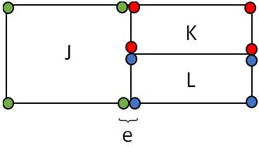
Figure 1: Example of two neighboring cells in a non-conforming mesh. The two green nodes from cell $J$, the two red nodes from cell $K$ and the two blue nodes from cell $L$ are involved in the computation of the flux in the boundary integral of (4) for face $e$.

3 Numerical results

We consider a number of two-dimensional benchmarks of atmospheric flows over orography for the validation of NWP codes, see e.g. the seminal papers [31, 32] and results and discussions in [5, 41, 48, 59]. The objective of these tests is twofold. First, we evaluate the stability and accuracy of numerical solutions obtained using non-conforming meshes compared to those obtained using uniform meshes. Second, we assess the computational cost carried by both setups and potential advantages at a given accuracy level.

Discrete parameter choices for the numerical simulations are associated with two Courant numbers, the acoustic Courant number $C$, based on the speed of sound $c$, and the advective Courant number $C_{u}$, based on the magnitude of the local flow velocity $u$:

$$C=rc\Delta t/{\mathcal{H}}\qquad C_{u}=ru\Delta t/{\mathcal{H}}.$$ (5)

Here $r$ is the polynomial degree used for the DG spatial discretization, $\mathcal{H}$ is the minimum cell diameter of the computational mesh, and $\Delta t$ is the time-step adopted for the time discretization. We consider polynomial degree $r=4$, unless differently stated. Wall boundary conditions are employed for the bottom boundary, whereas non-reflecting boundary conditions are required by the top boundary and the lateral boundaries. For this purpose, we introduce the following Rayleigh damping profile [41, 46]:

$$\lambda=\begin{cases}0,\qquad&\text{if }z<z_{B}\\ \overline{\lambda}\sin^{2}\left[\frac{\pi}{2}\left(\frac{z-z_{B}}{z-z_{T}}\right)\right]\qquad&\text{if }z\geq z_{B},\end{cases}$$ (6)

where $z_{B}$ denotes the height at which the damping starts and $z_{T}$ is the top height of the considered domain. Analogous definitions apply for the two lateral boundaries. The classical Gal-Chen height-based terrain-following coordinate [21] is used to obtain a terrain-following mesh in Cartesian coordinates.

A relevant diagnostic quantity to check that a correct orographic response is achieved is represented by the vertical flux of horizontal momentum (henceforth “momentum flux”), defined as [55]

$$m(z)=\int_{-\infty}^{\infty}\overline{\rho}(z)u^{\prime}(x,z)w^{\prime}(x,z)dx.$$ (7)

Here, $u^{\prime}$ and $w^{\prime}$ denote the deviation from the background state of the horizontal and vertical velocity, respectively. Table 1 reports the parameters employed for the different test cases.

Test case	$\boldsymbol{\Delta}\mathbf{t}$	$\mathbf{T_{f}}$	Domain	Damping	Damping	$\overline{\boldsymbol{\lambda}}\boldsymbol{\Delta}\mathbf{t}$	$\mathbf{C}$	$\mathbf{C_{u}}$
	$\boldsymbol{[}$\text{\,}\mathrm{s}$\boldsymbol{]}$	$\boldsymbol{[}$\text{\,}\mathrm{h}$\boldsymbol{]}$	$\boldsymbol{[}$\text{\,}\mathrm{km}$\times$\text{\,}\mathrm{km}$$$\boldsymbol{]}$	layer $\boldsymbol{(}x\boldsymbol{)}$	layer $\boldsymbol{(}z\boldsymbol{)}$
LHMW	2.5	15	$240\times 30$	(0,80), (160,240)	(15,30)	0.3	3.66	0.23
NLNHMW	1	5	$40\times 20$	(0,10), (30,40)	(9,20)	0.15	2.16	0.13
BWS	0.75	3	$220\times 25$	(0,30), (190,220)	(20,25)	0.15	0.79	0.23
T-REX	0.375	4	$400\times 25$	(0,50), (200,250)	(20,25)	0.15	0.8	0.13

Table 1: Model parameters for the test cases in this Section, see main text for details. LHMW: linear hydrostatic mountain wave. NLNHMW: nonlinear nonhydrostatic mountain wave. BWS: Boulder windstorm (inviscid configuration). T-REX: Sierra profile, T-REX experiment. The intervals where the damping layers are applied are in units of km.

3.1 Linear hydrostatic flow over a hill

First, we consider a linear hydrostatic configuration, see e.g. [24, 46]. The bottom boundary is described by the function

$$h(x)=\frac{h_{m}}{1+\left(\frac{x-x_{c}}{a_{c}}\right)^{2}},$$ (8)

the so-called versiera of Agnesi, with $h_{m}$ being the height of the hill and $a_{c}$ being its half-width. We take $h_{m}=$1\text{\,}\mathrm{m}$,x_{c}=$120\text{\,}\mathrm{km}$$, and $a_{c}=$10\text{\,}\mathrm{km}$$. The initial state of the atmosphere consists of a constant horizontal flow with $\overline{u}=$20\text{\,}\mathrm{m}\text{\,}{\mathrm{s}}^{-1}$$ and of an isothermal background profile with temperature $\overline{T}=$250\text{\,}\mathrm{K}$$ and Exner pressure:

$$\overline{\Pi}=\exp\left(-\frac{g}{c_{p}\overline{T}}z\right),$$ (9)

with $c_{p}=\frac{R\gamma}{\gamma-1}$ denoting the specific heat at constant pressure. In an isothermal configuration the Brunt-Väisälä frequency is given by $N=\frac{g}{\sqrt{c_{p}\overline{T}}}$. Hence, one can easily verify that

$$\frac{Na_{c}}{\overline{u}}\gg 1,$$ (10)

meaning that we are in a hydrostatic regime [24, 48]. The computational mesh is composed by $N_{el}=1116$ elements with 4 different refinement levels (Figure 2). The finest level corresponds to a resolution of $300\text{\,}\mathrm{m}$ along $x$ and of $62.5\text{\,}\mathrm{m}$ along $z$, whereas the coarsest level corresponds to a resolution of $2400\text{\,}\mathrm{m}$ along $x$ and of $500\text{\,}\mathrm{m}$ along $z$. From the linear theory, the analytical momentum flux is given by [55]

$$m^{H}=-\frac{\pi}{4}\overline{\rho}_{s}\overline{u}_{s}Nh_{m}^{2},$$ (11)

with $\overline{\rho}_{s}$ and $\overline{u}_{s}$ denoting the surface background density and velocity, respectively. The computed momentum flux normalized by $m^{H}$ approaches $1$ as the simulation reaches the steady state (Figure 3). The momentum is correctly transferred in the vertical direction and no spurious oscillations arise at the interface between different mesh levels.

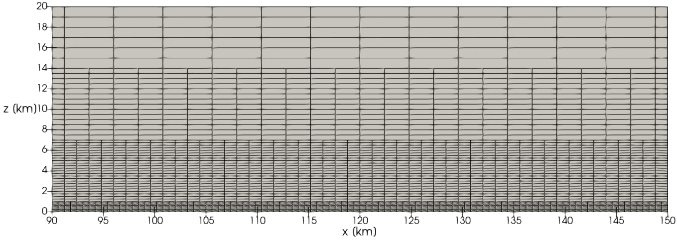
Figure 2: Linear hydrostatic flow over a hill, non-conforming mesh.

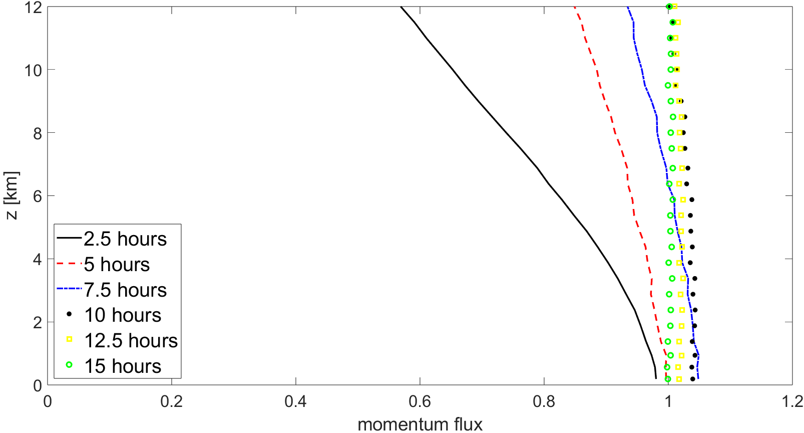
Figure 3: Linear hydrostatic flow over a hill, evolution of normalized momentum flux for the simulation using a non-conforming mesh.

A reference solution is computed using a uniform mesh with the maximum resolution of the non-conforming mesh, namely a mesh composed by $200$ elements along the horizontal direction and $120$ elements along the vertical one. A comparison of contour plots for the horizontal velocity deviation and for the vertical velocity shows an excellent agreement in the lee waves simulation between the uniform mesh at finer resolution and the non-conforming mesh (Figure 4).

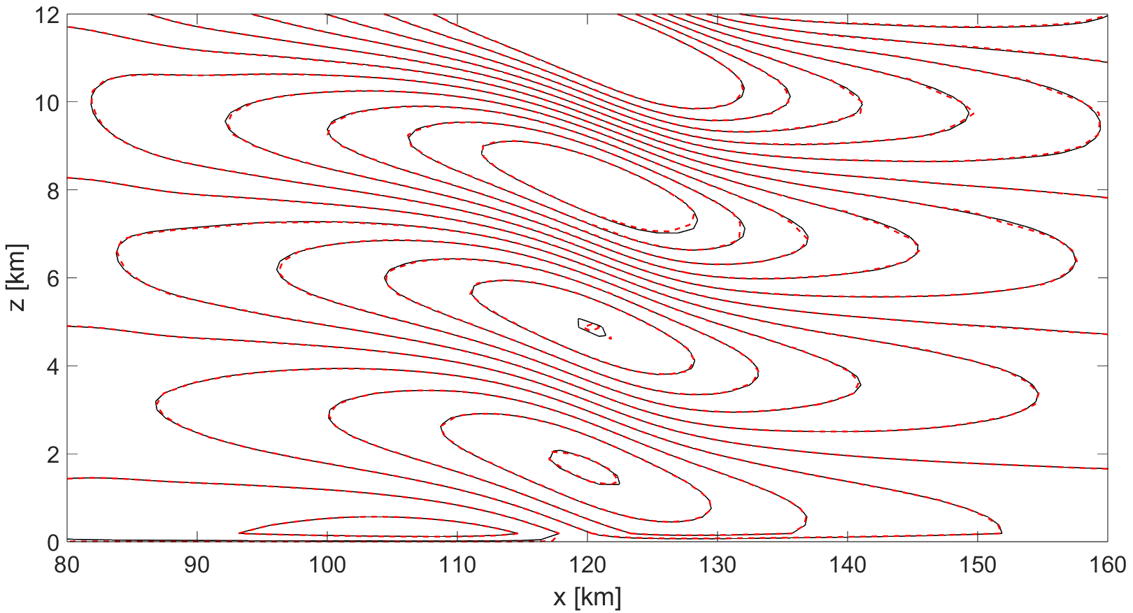
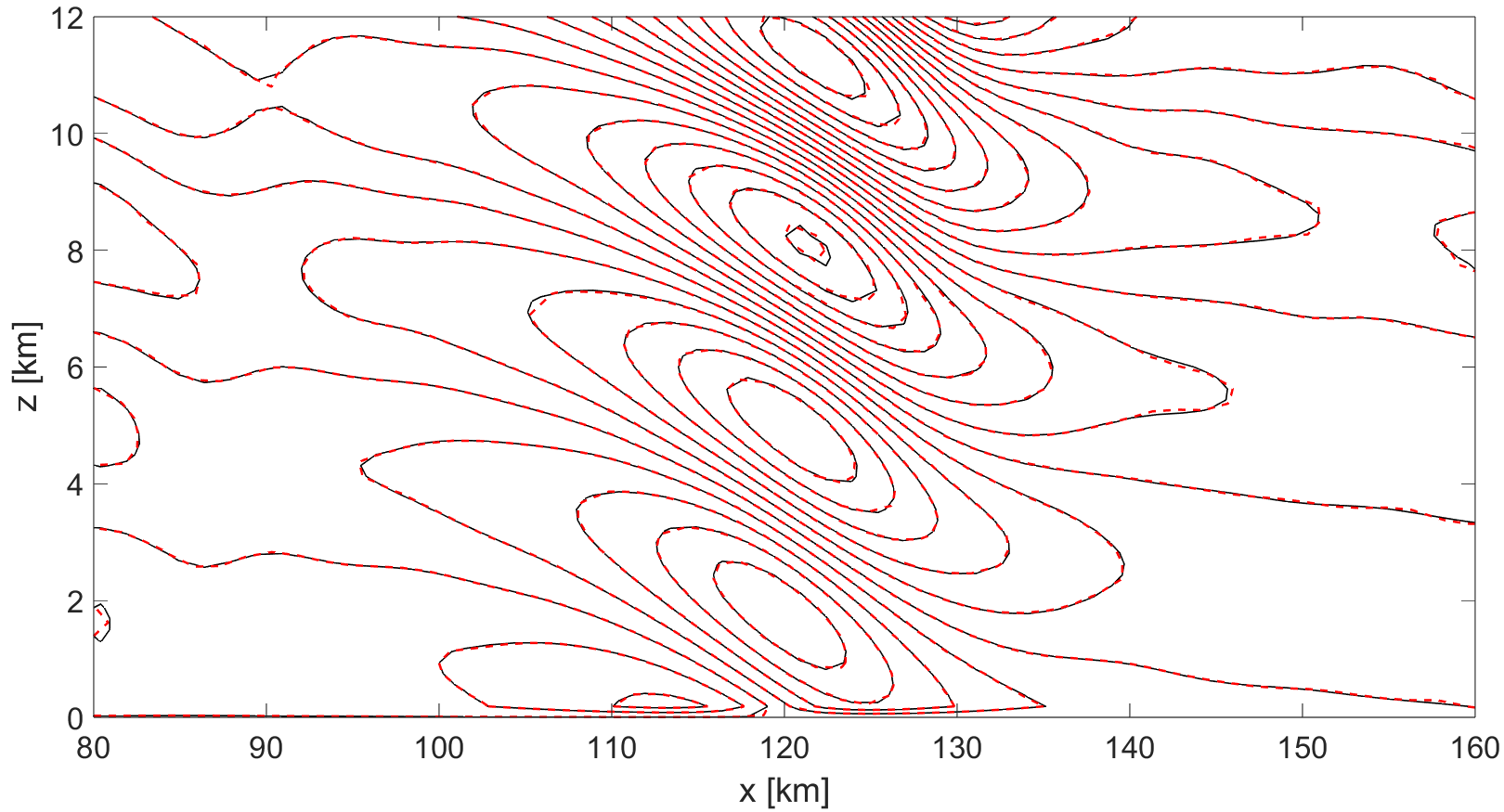
Figure 4: Linear hydrostatic flow over a hill at $t=T_{f}=$15\text{\,}\mathrm{h}$$, numerical solutions using a non-conforming mesh (solid black lines) and a uniform mesh at finer resolution (dashed red lines). Top: horizontal velocity deviation, contours in $[-2.5,2.5]\cdot 10^{-2}\text{\,}\mathrm{m}\text{\,}{\mathrm{s}}^{-1}$ with a $5\cdot 10^{-3}\text{\,}\mathrm{m}\text{\,}{\mathrm{s}}^{-1}$ contour interval; Bottom: vertical velocity, contours in $[-4,4]\cdot 10^{-2}\text{\,}\mathrm{m}\text{\,}{\mathrm{s}}^{-1}$ with a $5\cdot 10^{-4}\text{\,}\mathrm{m}\text{\,}{\mathrm{s}}^{-1}$ contour interval.

In order to further emphasize the results obtained with the use of the non-conforming mesh, we consider a uniform mesh with the same number of elements ($62\times 18$) of the non-conforming mesh. A three-way comparison of the normalized momentum computed with the uniform fine mesh, the uniform coarse mesh, and the non-conforming mesh shows a good agreement with the analytical solution $m^{H}$ (Figure 5). From a more quantitative point of view, we compute relative errors with respect to the reference solution in the portion of the domain $\Omega=$\left[80,160\right]\text{\,}\mathrm{km}$\times$\left[0,12\right]\text{\,}\mathrm{km}$$ (Table 2).

Moreover, we consider different configurations with non-conforming meshes and we compare them with configurations employing a uniform mesh using the same number of elements. Non-conforming mesh simulations significantly outperform uniform mesh simulations in terms of accuracy at a given number of degrees of freedom. At the finest $300\text{\,}\mathrm{m}$ horizontal resolution $62.5\text{\,}\mathrm{m}$ vertical resolution, the use of the non-conforming mesh leads to a computational time saving of around $90\%$ over the corresponding uniform mesh (bold numbers in Table 2). However, the present non-conforming mesh implementation is instead less competitive considering the wall-clock time at a given number of elements. This is due to the fact that, on non-conforming meshes, the condition number of the linear systems resulting from the IMEX discretization increases substantially, leading to a higher number of iterations for the GMRES solver [15, 29, 45]. While some effective geometric multigrid preconditioners are available for non-symmetric systems arising from elliptic equations [7, 18], their extension to hyperbolic problems and their implementation in the context of the matrix-free approach of the $\mathit{deal.II}$ library is not straightforward and will be the subject of future work.

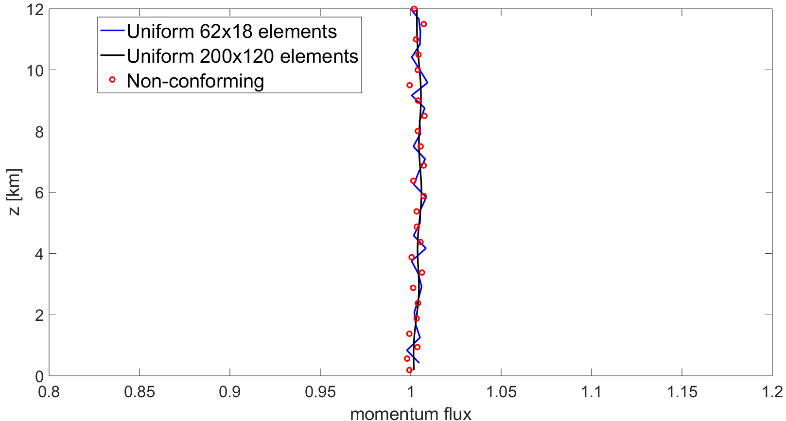
Figure 5: Linear hydrostatic flow over a hill, comparison of normalized momentum flux at $t=T_{f}=$15\text{\,}\mathrm{h}$$ obtained using a uniform mesh at fine resolution (solid black line), a uniform mesh with the same number of elements as the non-conforming mesh (solid blue line), and the non-conforming mesh (red dots). See text for mesh definitions.

$N_{el}$	Uniform				Non-conforming
	$\Delta x[$\text{\,}\mathrm{m}$]$	$\Delta z[$\text{\,}\mathrm{m}$]$	$l_{2}(m_{z})$	WT$[$\text{\,}\mathrm{s}$]$		$\Delta x_{\textrm{min}}[$\text{\,}\mathrm{m}$]$	$\Delta z_{\textrm{min}}[$\text{\,}\mathrm{m}$]$	$l_{2}(m_{z})$	WT$[$\text{\,}\mathrm{s}$]$
402	895.52	1250	$6.1010-2$	3050		1200	250	$4.3410-3$	4210
504	952.38	937.5	$1.9610-2$	3180		600	125	$2.3410-3$	6510
1116	967.74	416.67	$3.9410-3$	4470		300	62.5	$2.5310-3$	14800
24000	300	62.5	-	131600		-	-	-	-

Table 2: Linear hydrostatic flow over a hill: horizontal resolution $\Delta x$, vertical resolution $\Delta z$, $l^{2}$ relative errors on the momentum flux, and wall-clock times (WT) for the uniform meshes and the non-conforming meshes. Here, and in the following tables, $N_{el}$ denotes the number of elements.

3.2 Nonlinear non-hydrostatic flow over a hill

Next, we consider a non-hydrostatic regime for which

$$\frac{Na_{c}}{\overline{u}}\approx 1.$$ (12)

More specifically, we focus on a nonlinear non-hydrostatic case [46, 50, 59]. The bottom boundary is described again by (8), with $h_{m}=$450\text{\,}\mathrm{m}$,x_{c}=$20\text{\,}\mathrm{km}$$, and $a_{c}=$1\text{\,}\mathrm{km}$$. The initial state of the atmosphere is described by a constant horizontal flow with $\overline{u}=$13.28\text{\,}\mathrm{m}\text{\,}{\mathrm{s}}^{-1}$$ and by the following potential temperature and Exner pressure:

$$\overline{\theta} = \theta_{ref}\exp\left(\frac{N^{2}}{g}z\right)$$ (13)

$$\overline{\Pi} = 1+\frac{g^{2}}{c_{p}\theta_{ref}N^{2}}\left[\exp\left(-\frac{N^{2}}{g}z\right)-1\right],$$ (14)

with $\theta_{ref}=$273\text{\,}\mathrm{K}$$ and $N=$0.02\text{\,}{\mathrm{s}}^{-1}$$. The mesh is composed by $N_{el}=282$ elements with $3$ different resolution levels (Figure 6). The finest level corresponds to a resolution of $208.33\text{\,}\mathrm{m}$ along $x$ and of $104.17\text{\,}\mathrm{m}$ along $z$, whereas the coarsest level corresponds to a resolution of around $833.33\text{\,}\mathrm{m}$ along $x$ and of $416.67\text{\,}\mathrm{m}$ along $z$.

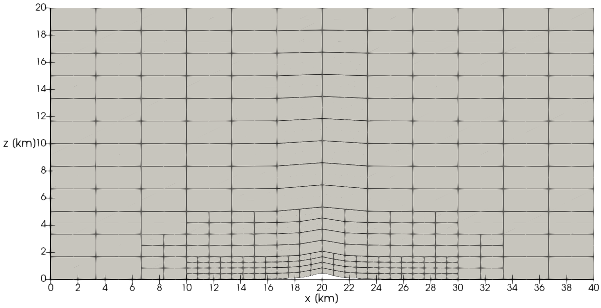
Figure 6: Nonlinear non-hydrostatic flow over a hill, non-conforming mesh.

A reference solution is computed using a uniform mesh with $48\times 48$ elements, which corresponds to the finest resolution of the non-conforming mesh. A comparison of contour plots for the horizontal velocity deviation and for the vertical velocity shows good agreement between the uniform mesh at finer resolution and the non-conforming mesh in the development of lee waves (Figure 7). The use of the non-conforming mesh yields a computational time saving of around $60\%$ (bold numbers in Table 3). In addition, we consider a mesh with uniform resolution and with the same number of elements $47\times 6$ of the non-conforming mesh. We compare the computed normalized momentum flux at $t=T_{f}$ in the reference configuration, in the non-conforming mesh configuration, and in the configuration with a uniform mesh with the same number of elements of the non-conforming mesh (Figure 8). In terms of relative error with respect to the reference solution, the locally refined non-conforming mesh outperforms the uniform mesh by about an order of magnitude using the same number of elements (Table 3). Analogous considerations to those reported in Section 3.1 are valid for the computational time.

$N_{el}$	$\Delta x[$\text{\,}\mathrm{m}$]$	$\Delta z[$\text{\,}\mathrm{m}$]$	$l_{2}(m_{z})$	WT$[$\text{\,}\mathrm{s}$]$
282 (uniform)	212.77	833.33	$2.3110-1$	4520
282 (non-conforming)	208.33	104.17	$2.3410-2$	9680
2304 (uniform)	208.33	104.17	-	22500

Table 3: Nonlinear non-hydrostatic flow over a hill: horizontal resolution $\Delta x$, vertical resolution $\Delta z$, $l^{2}$ relative errors on the momentum flux, and wall-clock times (WT) for the uniform meshes and the non-conforming mesh.

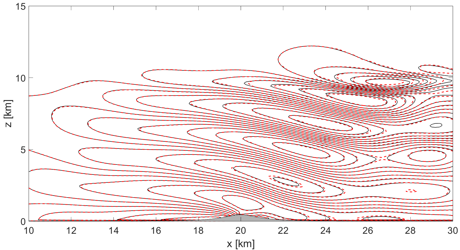
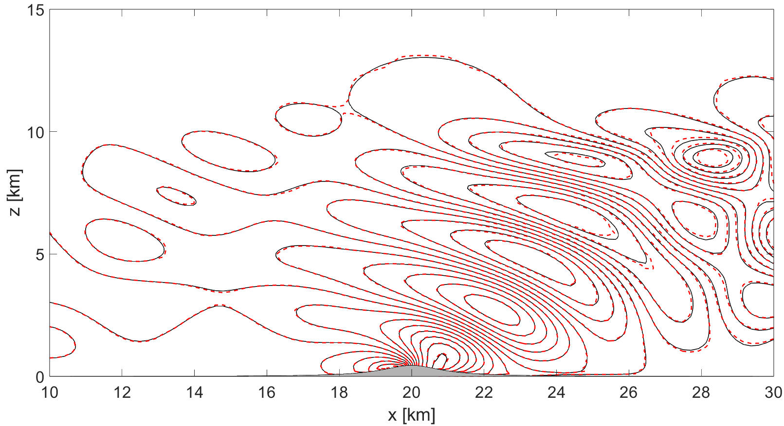
Figure 7: Nonlinear non-hydrostatic flow over a hill at $t=T_{f}=$5\text{\,}\mathrm{h}$$, computed on a uniform mesh at finer resolution (solid black lines) and on a non-conforming mesh (dashed red lines). Top: horizontal velocity deviation, contours in the interval $[-7.2,9.0]\text{\,}\mathrm{m}\text{\,}{\mathrm{s}}^{-1}$ with a $1.16\text{\,}\mathrm{m}\text{\,}{\mathrm{s}}^{-1}$ interval. Bottom: vertical velocity, contours in the interval $[-4.2,4.0]\text{\,}\mathrm{m}\text{\,}{\mathrm{s}}^{-1}$ with a $0.586\text{\,}\mathrm{m}\text{\,}{\mathrm{s}}^{-1}$ interval.

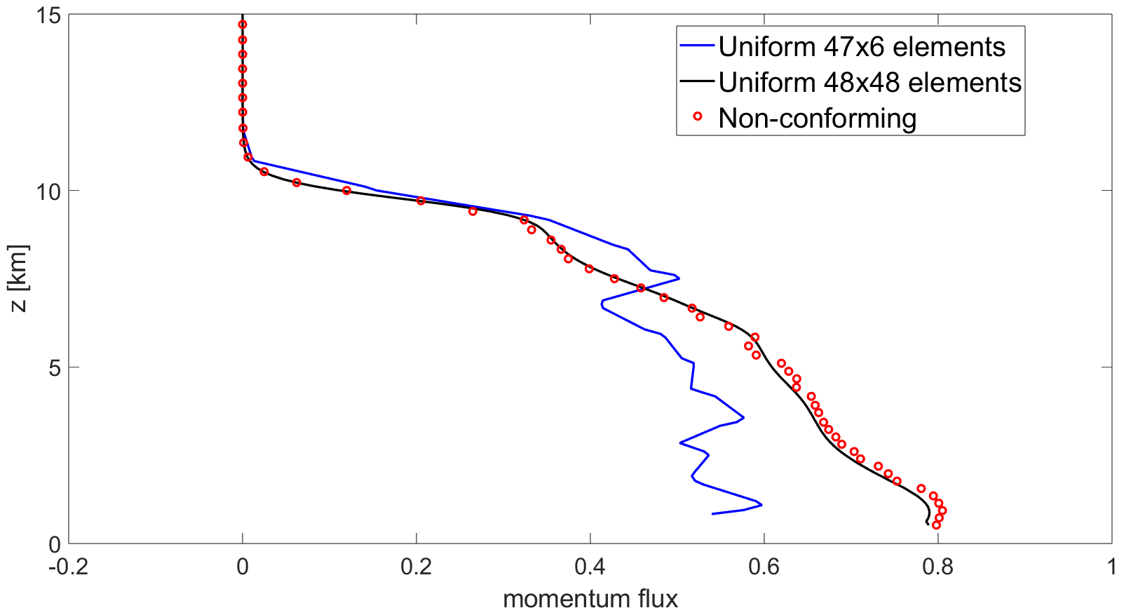
Figure 8: Nonlinear non-hydrostatic flow over a hill, comparison of normalized momentum flux at $t=T_{f}=$5\text{\,}\mathrm{h}$$ obtained using a uniform mesh at fine resolution (black solid line), a uniform mesh with the same number of elements of the non-conforming mesh (blue solid line), and the non-conforming mesh (red dots).

3.3 11 January 1972 Boulder Windstorm

Next, we consider the more realistic orography profile for the 11 January 1972 Boulder (Colorado) windstorm benchmark [14]. This test case is particularly challenging because a complex wave-breaking response is established aloft in the lee of the mountain. The initial conditions are horizontally homogeneous and based upon the upstream measurements at 1200 UTC 11 January 1972 Grand Junction, Colorado, as shown in [14]. The initial conditions contain a critical level near $z=$21\text{\,}\mathrm{km}$$ (Figure 9), which more realistically simulates the stratospheric gravity wave breaking [14]. The pressure is computed from the hydrostatic balance, namely

$$p(z)=p_{0}\exp{\left(-\frac{g}{R}\int_{0}^{z}\frac{1}{T(s)}ds\right)},$$ (15)

with $p_{0}=$10^{5}\text{\,}\mathrm{Pa}$$. Linear interpolation is employed to evaluate both temperature and horizontal velocity.

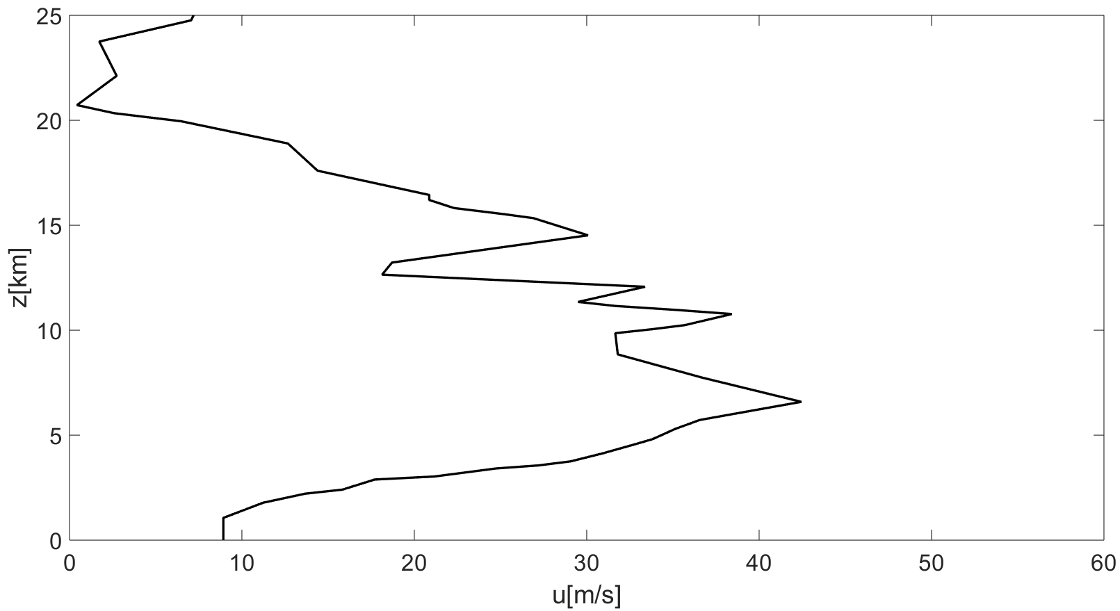
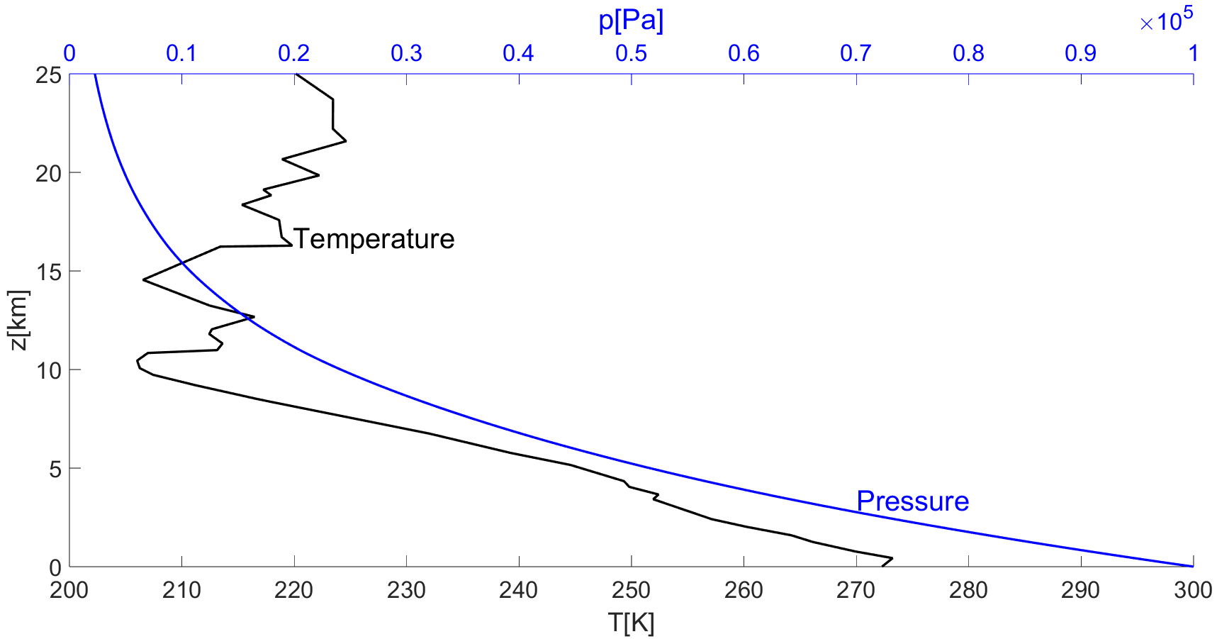
Figure 9: Boulder windstorm test case, initial conditions. Top: horizontal velocity. Bottom: temperature (black line) and pressure (blue line).

The bottom boundary is described by (8), with $h_{m}=$2\text{\,}\mathrm{km}$,x_{c}=$100\text{\,}\mathrm{km}$,$ and $a_{c}=$10\text{\,}\mathrm{km}$$. We consider two different computational meshes: a uniform mesh composed by $120\times 60$ elements, i.e. a resolution of $458.33\text{\,}\mathrm{m}$ along the horizontal direction and of $104.17\text{\,}\mathrm{m}$ along the vertical one, and a non-conforming mesh with 3 different levels, composed by $N_{el}=1524$ (Figure 10), with the finest level corresponding to the resolution of the uniform mesh.

The horizontal velocity and the potential temperature computed at $t=T_{f}$ by the IMEX-DG method using a uniform mesh are in reasonable agreement with the reference results [14], in particular for what concerns the potential temperature (Figure 11). Numerous regions of small-scale motion and larger high-frequency spatial structures arise with respect to the other tests using the uniform mesh, because of the lack of a subgrid eddy viscosity. The qualitative behaviour of the simulation with the uniform mesh and the one with the non-conforming mesh is in good agreement, even though visible differences arise in the deep regions of wave breaking in the stratosphere (Figure 11). In terms of wall-clock time, the configuration with the non-conforming mesh is about $65\%$ computationally cheaper than the configuration with the uniform mesh ($3.75\times 10^{4}\text{\,}\mathrm{s}$ vs. $1.37\times 10^{4}\text{\,}\mathrm{s}$).

Following [13], we then compute the momentum flux (7) using the mean value of $u$ and $w$ to compute $u^{\prime}$ and $w^{\prime}$. A comparison at final time of the vertical flux of horizontal momentum (7) normalized by its values at the surface obtained with the uniform mesh displays a reasonable agreement between the two simulations, especially for $z$ above $12\text{\,}\mathrm{km}$ (Figure 12). The discrepancy in the vertical region between $z=$7\text{\,}\mathrm{km}$$ and $z=$12\text{\,}\mathrm{km}$$ is probably due to the development of small-scale features and to the lack of subgrid eddy viscosity parametrization, as already discussed for the contour plots.

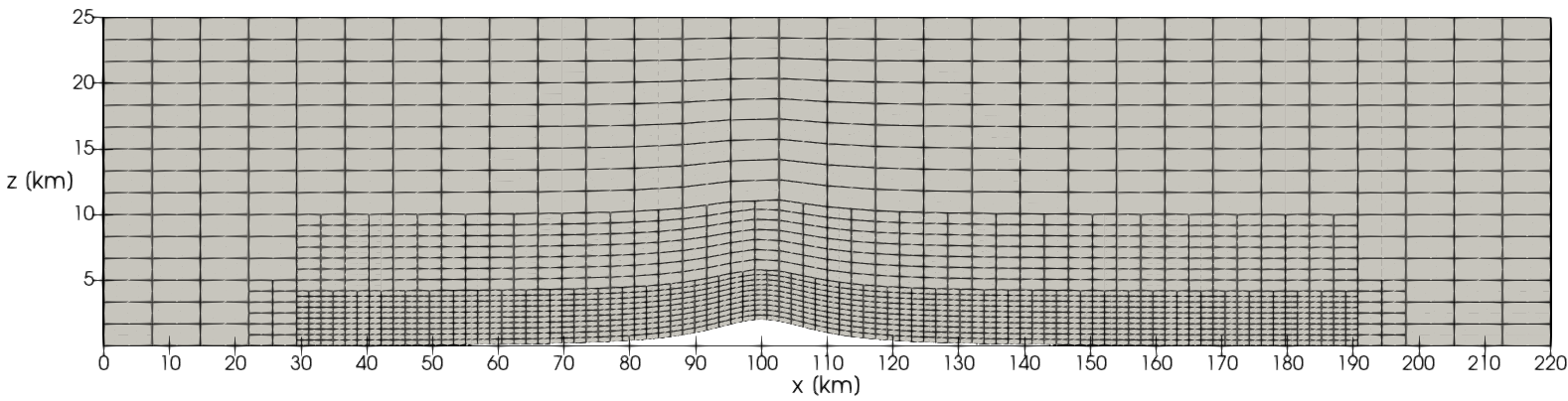
Figure 10: Boulder windstorm test case, non-conforming mesh.

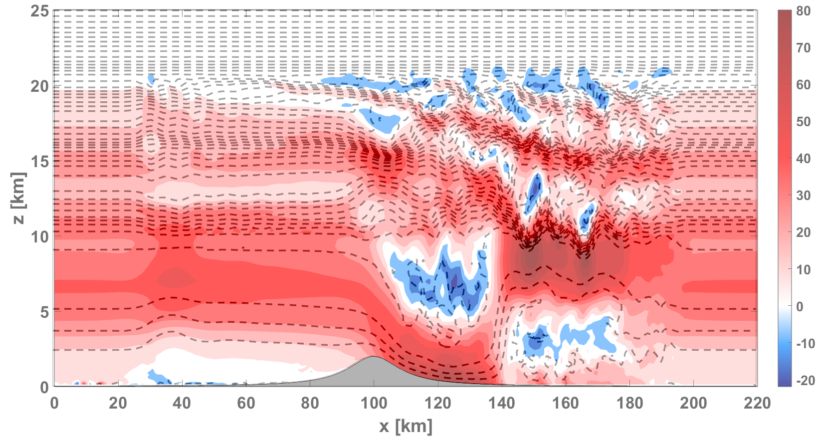
Figure 11: Boulder windstorm test case numerical results at $t=T_{f}=$3\text{\,}\mathrm{h}$$. Top: uniform mesh. Bottom: non-conforming mesh. Horizontal velocity (colors), contours in the range $[-40,80]\text{\,}\mathrm{m}\text{\,}{\mathrm{s}}^{-1}$ with a $8\text{\,}\mathrm{m}\text{\,}{\mathrm{s}}^{-1}$ interval. Potential temperature (dashed lines), contours in the range $[273,650]\text{\,}\mathrm{K}$ with an $8\text{\,}\mathrm{K}$ interval.

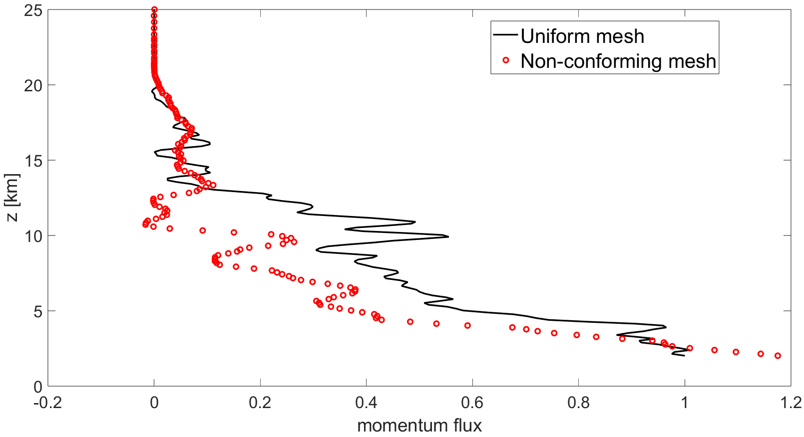
Figure 12: Boulder windstorm test case, comparison of normalized momentum flux at $t=T_{f}=$3\text{\,}\mathrm{h}$$ computed using the uniform mesh (solid black line) and the non-conforming mesh (red dots).

Next, we repeat the simulations for this test case including a simplified model for turbulent vertical diffusion for NWP applications, originally proposed in [38] and also discussed in [4, 6, 25]. As commonly done in numerical models for atmospheric physics, we resort to an operator splitting approach. The diffusion model is treated with the implicit part of the IMEX method, which corresponds to the TR-BDF2 scheme [27, 45]. The non-linear diffusivity $\kappa$ has the form

$$\kappa\left(\frac{\partial u}{\partial z},\frac{\partial\theta}{\partial z}\right)=l^{2}\left|\frac{\partial u}{\partial z}\right|F\left(Ri\right).$$ (16)

Here, $l$ is a mixing length and $Ri$ is the Richardson number given by

$$Ri=\frac{g}{\theta_{0}}\frac{\frac{\partial\theta}{\partial z}}{\left|\frac{\partial u}{\partial z}\right|^{2}},$$ (17)

with $\theta_{0}$ denoting a reference temperature. Finally, the function $F\left(Ri\right)$ is defined as

$$F\left(Ri\right)=\left(1+b\left|Ri\right|\right)^{\beta},$$ (18)

where

$$\begin{cases}\beta=-2,b=5\qquad&\text{if }Ri>0\\ \beta=\frac{1}{2},b=20\qquad&\text{if }Ri<0.\end{cases}$$ (19)

We consider the uniform mesh with $120\times 60$ elements and a coarse non-conforming mesh with $N_{el}=1524$ elements already employed for the inviscid case. In addition, we consider a fine non-conforming mesh with three different refinement levels and $N_{el}=6324$ elements. The fine resolution around the orography is of $229.17\text{\,}\mathrm{m}$ along the horizontal direction and of $52.08\text{\,}\mathrm{m}$ along the vertical one. We use a time step $\Delta t=$0.375\text{\,}\mathrm{s}$$, corresponding to a maximum acoustic Courant number $C\approx 0.79$ and a maximum advective Courant number $C_{u}\approx 0.23$. Finally, we take $l=$100\text{\,}\mathrm{m}$$ and $\theta_{0}=$273\text{\,}\mathrm{K}$$ in (16).

At $t=T_{f}$, numerical solutions computed using the uniform mesh and the non-conforming mesh are in good agreement for both the horizontal velocity and the potential temperature, in particular for the finer non-conforming mesh (Figure 13). In terms of wall-clock time, a computational time saving of around $50\%$ is achieved with the coarse non-conforming mesh (bold numbers in Table 4), while performance is less optimal for the fine non-conforming mesh (see the discussion above in Section 3.1). Finally, a comparison at $t=T_{f}$ of the computed momentum flux (7) normalized by its values at the surface obtained with the uniform mesh shows that the results of the uniform mesh are approached as long as the resolution of the non-conforming mesh increases (Figure 14).

$N_{el}$	$\Delta x[$\text{\,}\mathrm{m}$]$	$\Delta z[$\text{\,}\mathrm{m}$]$	WT$[$\text{\,}\mathrm{s}$]$
7200 (uniform)	458.33	104.17	119000
1524 (non-conforming)	229.17	104.17	51900
6324 (non-conforming)	229.17	52.08	160000

Table 4: Boulder windstorm test case with turbulent vertical diffusion: horizontal resolution $\Delta x$, vertical resolution $\Delta z$, and wall-clock times (WT) for the uniform meshes and the non-conforming mesh.

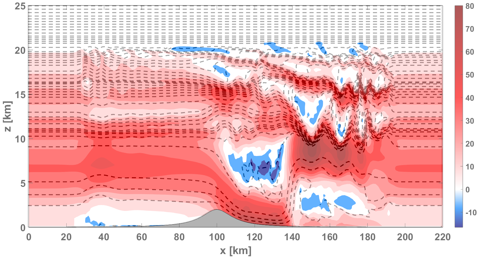
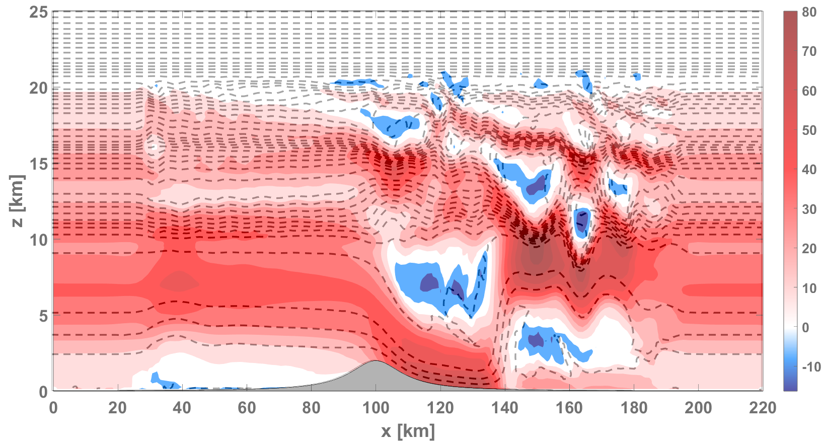
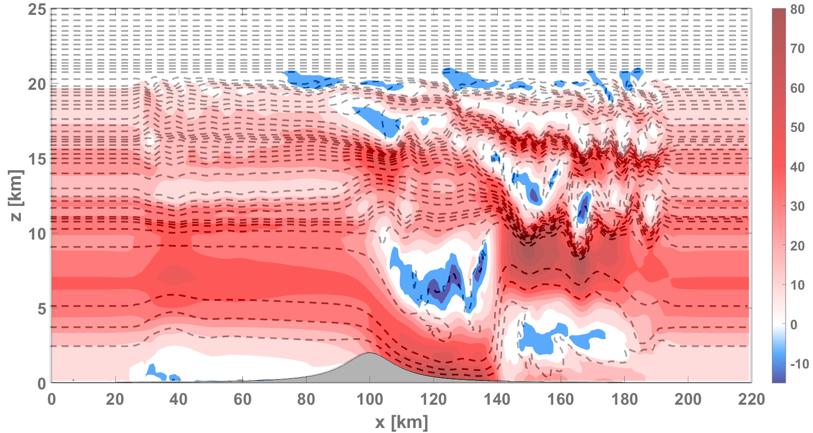
Figure 13: Boulder windstorm test case with turbulent vertical diffusion. Top: uniform mesh. Middle: coarse non-conforming mesh. Bottom: fine non-conforming mesh. Horizontal velocity (colors), contours in the range $[-40,80]\text{\,}\mathrm{m}\text{\,}{\mathrm{s}}^{-1}$ with a $8\text{\,}\mathrm{m}\text{\,}{\mathrm{s}}^{-1}$ interval. Potential temperature (dashed lines), contours in the range $[273,650]\text{\,}\mathrm{K}$ with an $8\text{\,}\mathrm{K}$ interval.

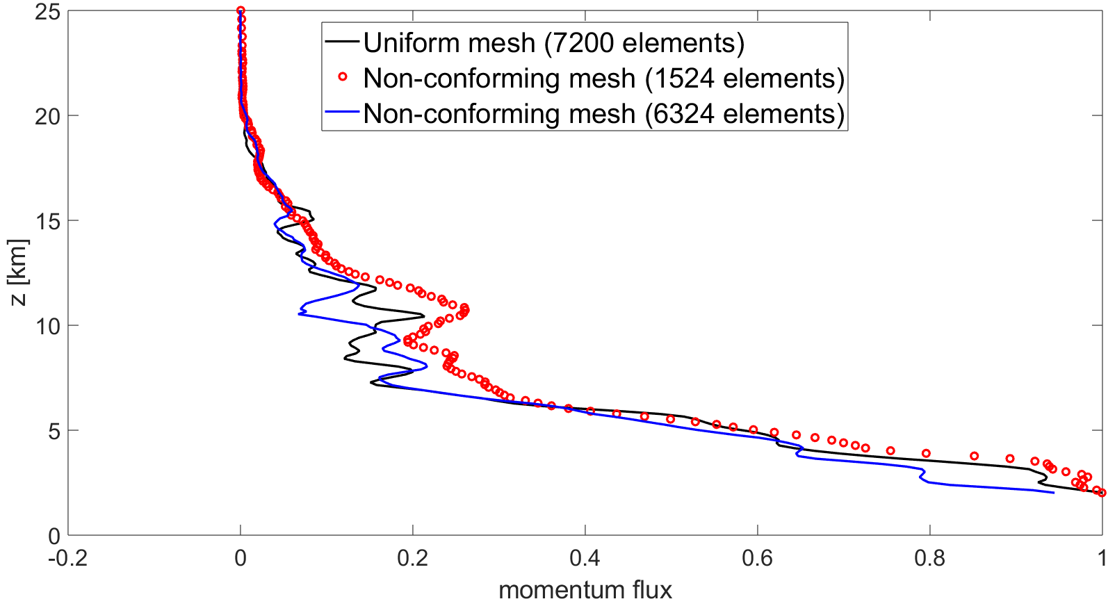
Figure 14: Boulder windstorm test case, comparison of normalized momentum flux at $t=T_{f}=$3\text{\,}\mathrm{h}$$ between the uniform mesh (solid black line), the fine (blue solid line), and the coarse (red dots) non-conforming meshes.

3.4 T-REX Mountain-Wave

In a final test, we consider simulations of a flow over a steep real orography [13, 34], as shown in Figure 15. The initial state is horizontally homogeneous and it is based on conditions during Intensive Observation Period (IOP) 6 of the Terrain-Induced Rotor Experiment (T-REX) [13], as reported in Figure 16. We consider a DG spatial discretization using degree $r=2$ polynomials and three computational meshes: a uniform mesh composed by $400\times 60$ elements, corresponding to a resolution of $500\text{\,}\mathrm{m}$ along the horizontal direction and of $208.33\text{\,}\mathrm{m}$ along the vertical direction, and two non-conforming meshes. The coarsest non-conforming mesh consists of three different levels and $N_{el}=5742$ elements, whereas the finest non-conforming mesh is obtained with a global refinement of the coarsest non-conforming mesh, with $N_{el}=22968$ elements (Figure 17). The finest level of the coarser non-conforming mesh corresponds to the resolution of the uniform mesh. Hence, the fine resolution around the orography for the finest non-conforming mesh is $250\text{\,}\mathrm{m}$ along the horizontal direction and $104.17\text{\,}\mathrm{m}$ along the vertical one. We take $l=$100\text{\,}\mathrm{m}$$ and $\theta_{0}=$273\text{\,}\mathrm{K}$$ in (16). The vertical turbulent diffusion model is necessary to obtain a stable numerical solution.

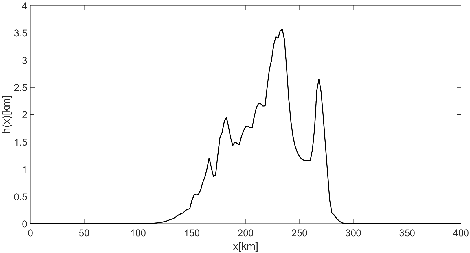
Figure 15: T-REX mountain-wave test, Sierra profile.

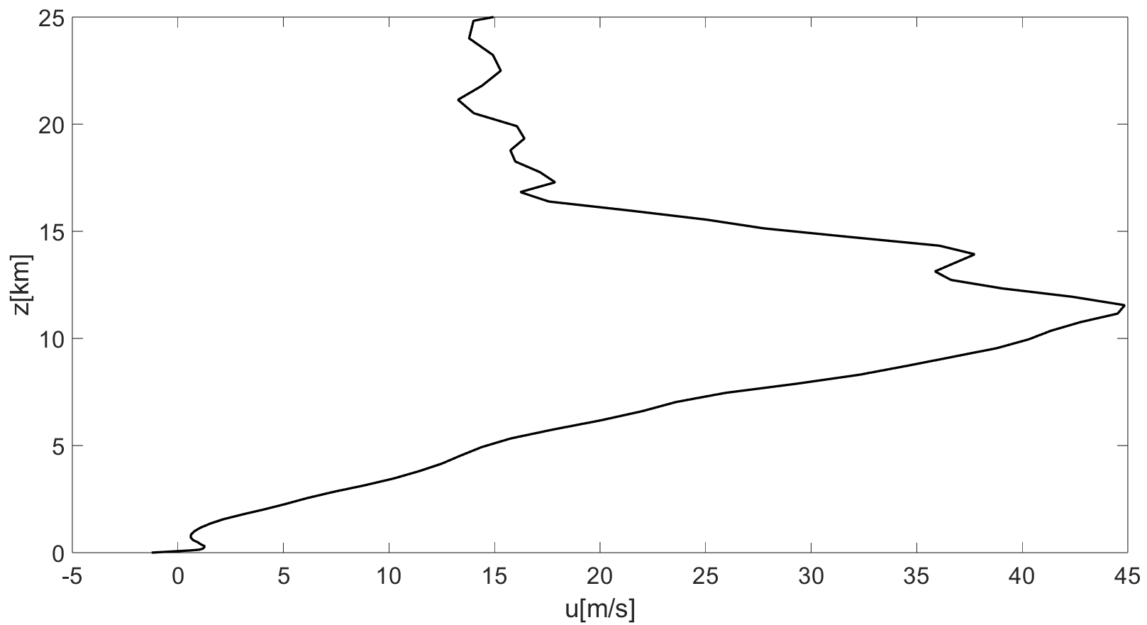
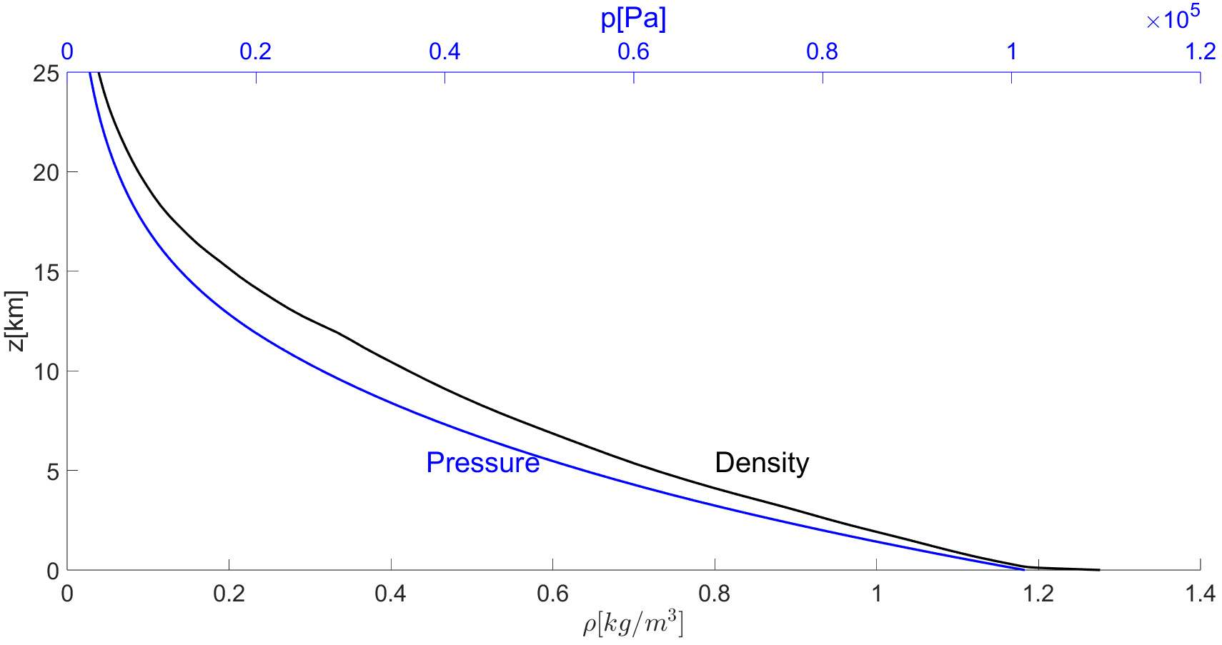
Figure 16: T-REX mountain-wave test case, initial conditions. Top: horizontal velocity. Bottom: density (black line) and pressure (blue line).

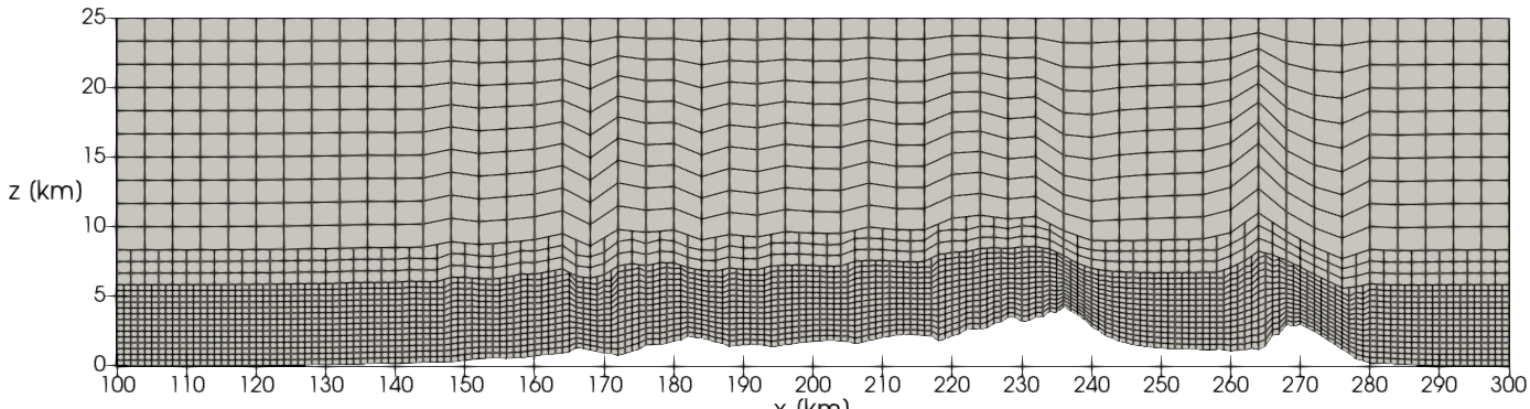
Figure 17: T-REX mountain wave, non-conforming mesh.

The IMEX-DG numerical solutions at $t=T_{f}$ display good agreement both in the horizontal velocity and in the potential temperature variables between the uniform mesh and the non-conforming meshes, showing even for a real steep orography the robustness of the method in the use of non-conforming meshes (Figure 18). While some differences arise in the structures of the horizontal velocity, unlike the previous test case, there is low predictability of key characteristics such as the strength of downslope winds or the stratospheric wave breaking in this benchmark [13]. Moreover, the change in the resolution of the topography has been shown to modify the representation of mountain wave-driven middle atmosphere processes [30]. We remark that the results in Figure 18 show notable differences with respect to those reported in [13] likely due to differences in the employed configuration.

A far-field comparison of the momentum flux (7) normalized with the value obtained at $z=$7\text{\,}\mathrm{km}$$ for the uniform mesh solution confirms the low predictability of large-scale orographic features for this test case (Figure 19). In this case, the uniform mesh is the configuration characterized by the lowest wall-clock time (Table 5). As already discussed in Section 3.1, this is related to the increase of the condition number for the linear systems to be solved when non-conforming meshes are used.

$N_{el}$	$\Delta x[$\text{\,}\mathrm{m}$]$	$\Delta z[$\text{\,}\mathrm{m}$]$	WT$[$\text{\,}\mathrm{s}$]$
24000 (uniform)	500	208.33	165000
5742 (non-conforming)	500	208.33	172000
22698 (non-conforming)	250	104.17	374000

Table 5: T-REX mountain wave test case: horizontal resolution $\Delta x$, vertical resolution $\Delta z$, and wall-clock times (WT) for the uniform meshes and the non-conforming mesh.

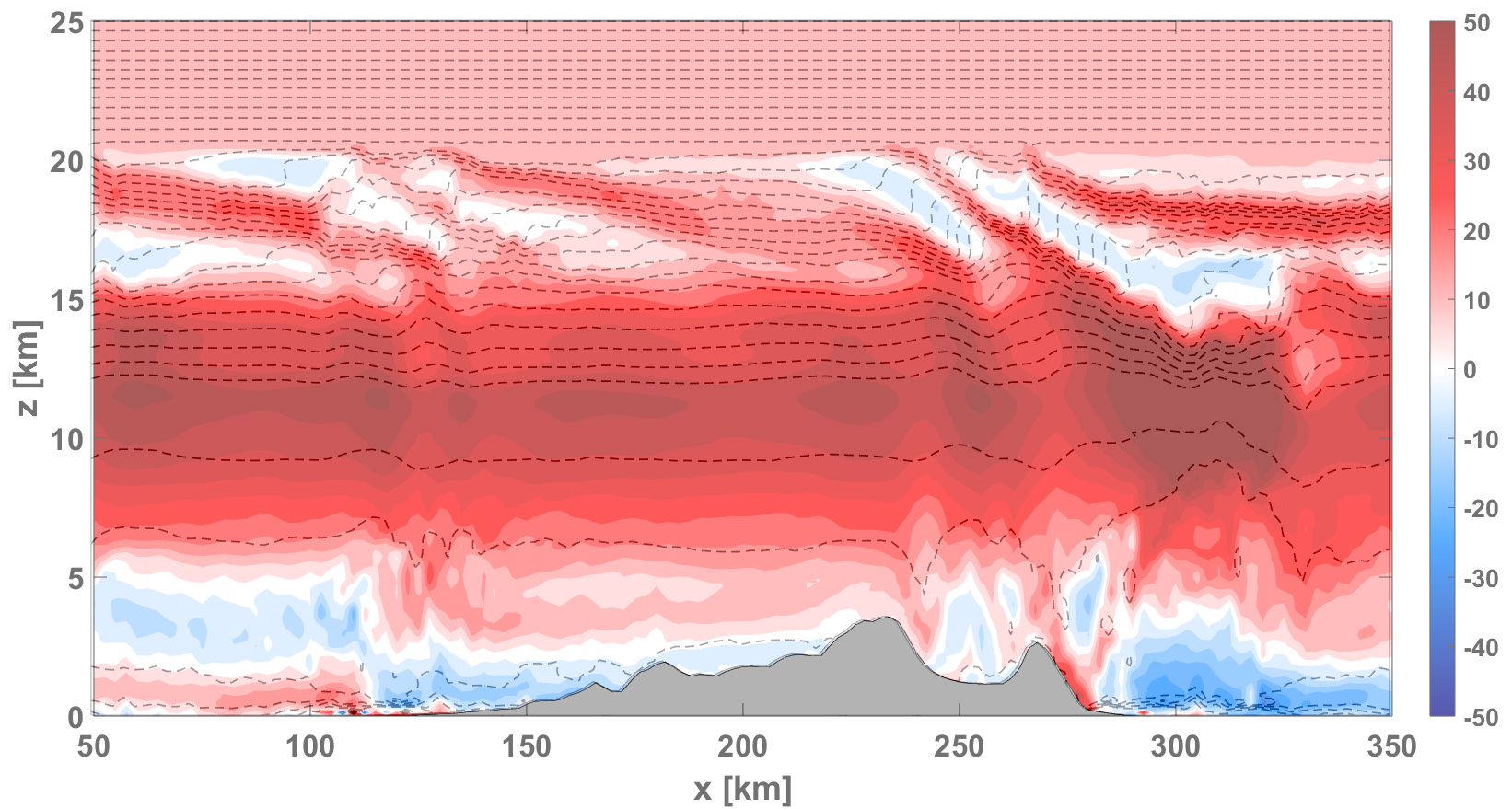
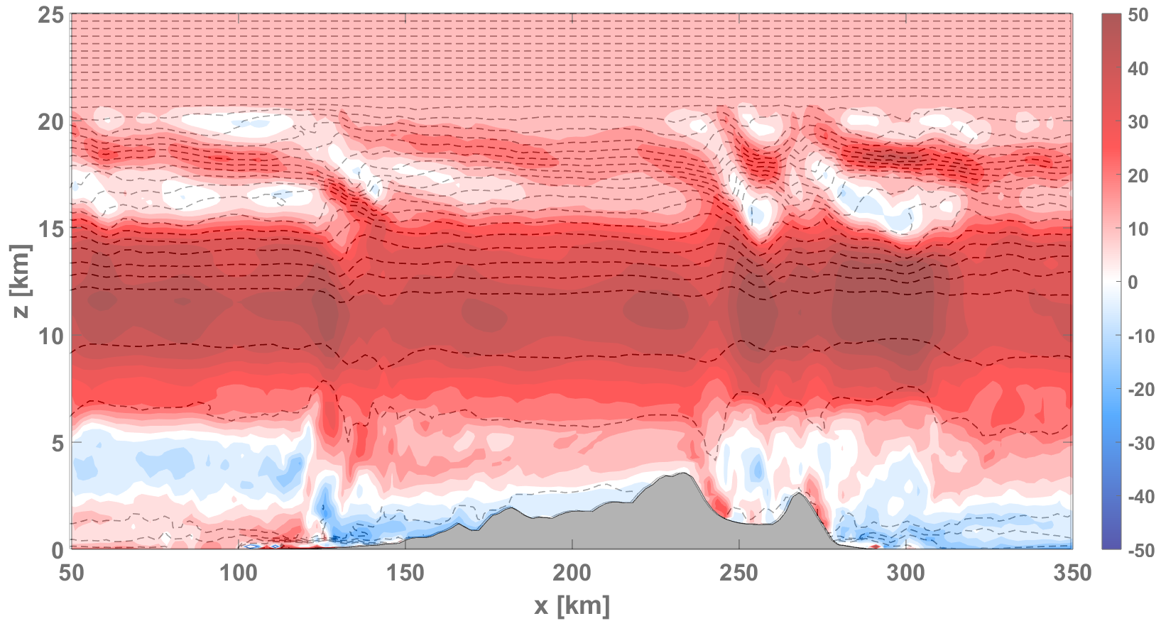
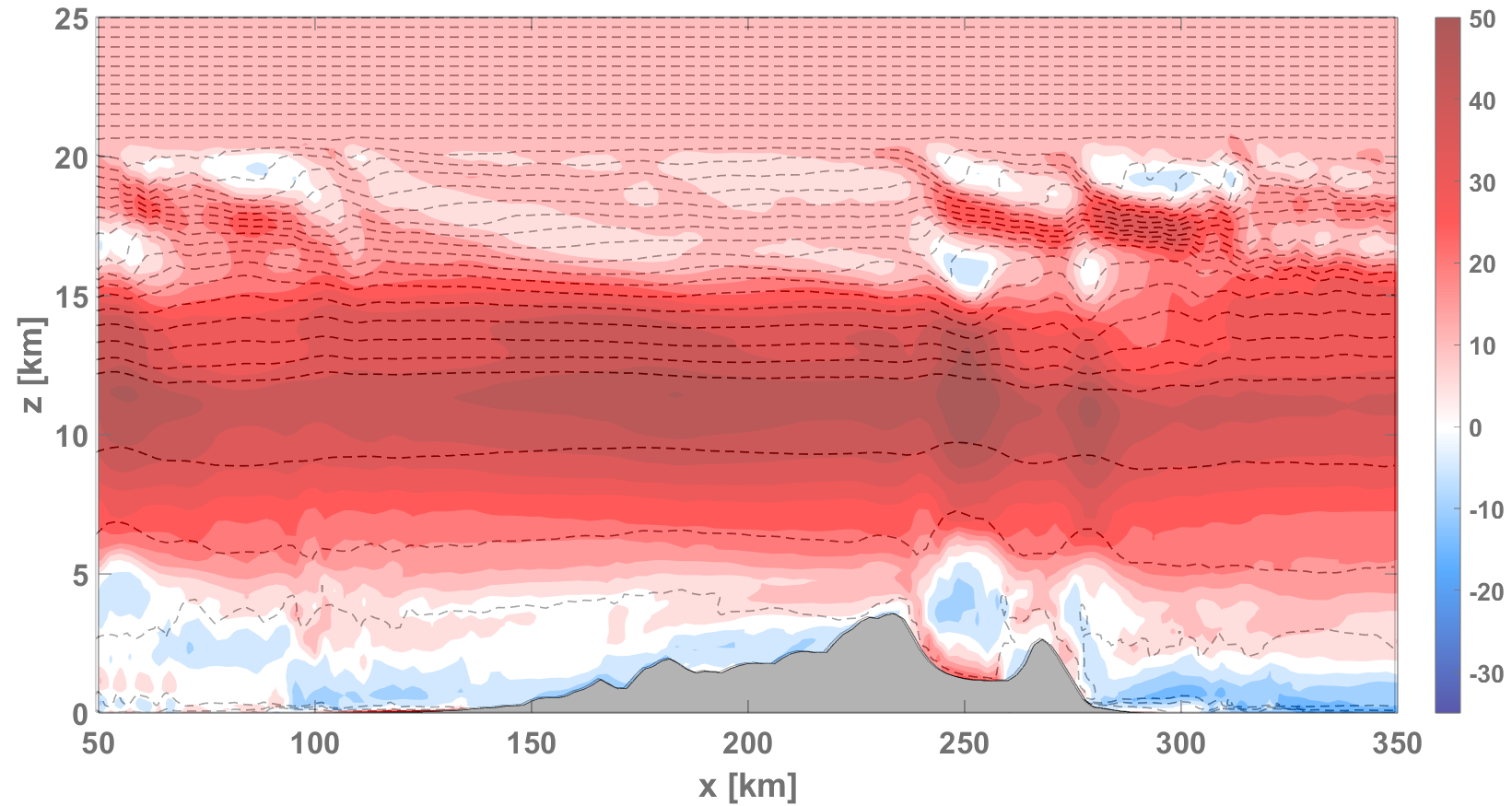
Figure 18: T-REX mountain wave test case at $T_{f}=$4\text{\,}\mathrm{h}$$. Top: uniform mesh. Middle: coarsest non-conforming mesh. Bottom: finest non-conforming mesh. Horizontal velocity perturbation (colors), contours in the range$[-30,30]\text{\,}\mathrm{m}\text{\,}{\mathrm{s}}^{-1}$ with a $2.5\text{\,}\mathrm{m}\text{\,}{\mathrm{s}}^{-1}$ interval. Potential temperature (dashed lines), contours in the range $[273,650]\text{\,}\mathrm{K}$ with a $10\text{\,}\mathrm{K}$ interval.

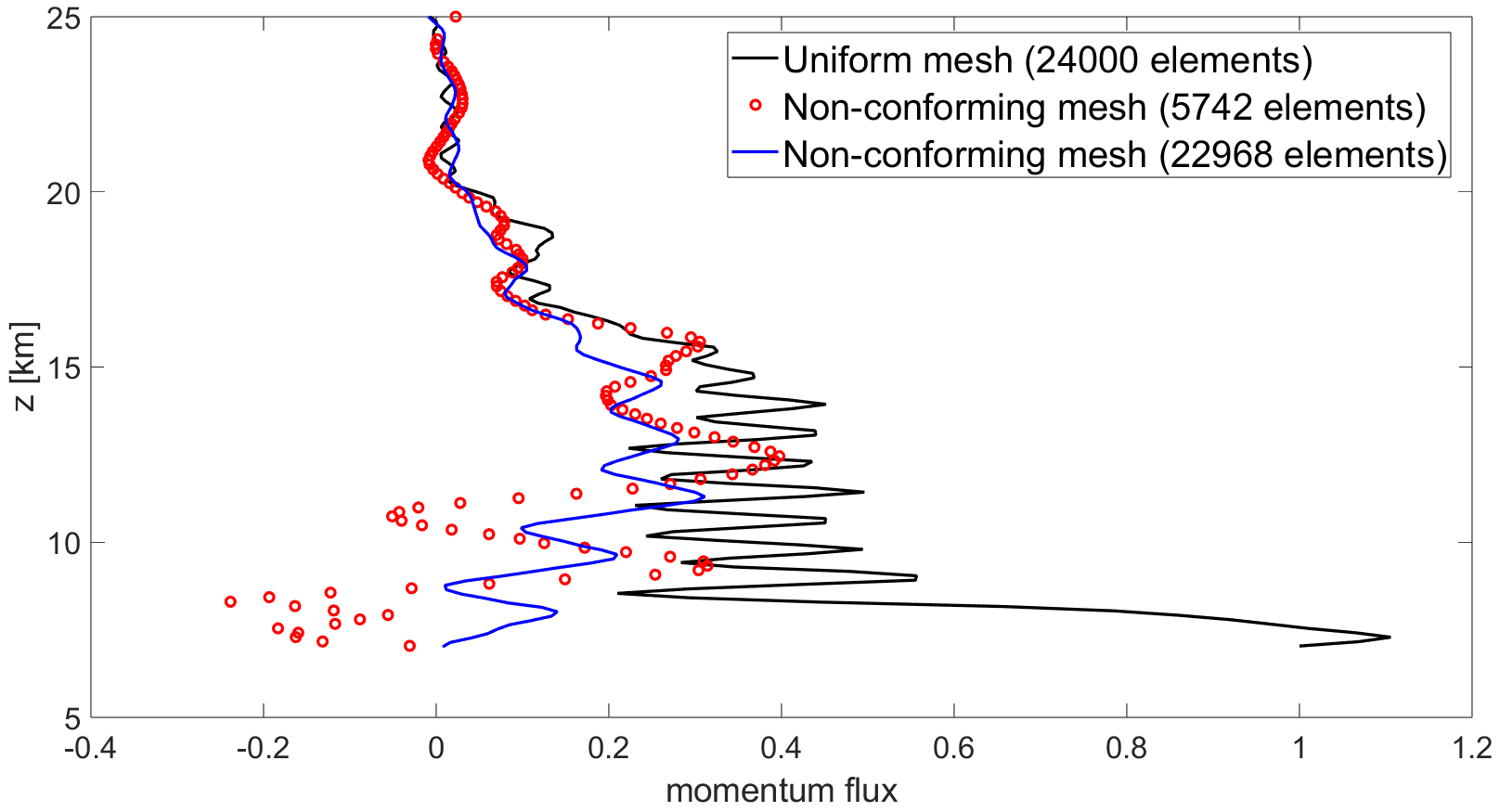
Figure 19: T-REX mountain wave test case, comparison of normalized momentum flux at $t=T_{f}=$4\text{\,}\mathrm{h}$$ between the uniform mesh (solid black line), the finer non-conforming mesh (blue line), and the coarser non-conforming mesh (red dots).

4 Conclusions

We have presented a systematic assessment of non-conforming meshes for the simulation of flows over orography using an IMEX-DG numerical model for the compressible Euler equations. For this purpose, we have exploited the adaptation framework provided by the open-source numerical library $\mathit{deal.II}$ [1, 3]. At a given accuracy level, the use of non-conforming meshes enables a significant reduction in the number of computational degrees of freedom with respect to uniform resolution meshes. The numerical results show that stable simulations are produced with no spurious reflections at internal boundaries separating mesh regions with different resolutions. In addition, accurate values for the momentum flux are retrieved in robust non-conforming simulations for increasingly realistic orography profiles.

Numerical simulations with non-conforming meshes can use substantially higher resolution only near the orographic features, correctly reproducing the larger scale, far-field orographic response, while using meshes that are relatively coarse over most of the domain. The results obtained in our framework envisage the use of locally refined, non-conforming meshes as a reliable, effective tool to push NWP and climate models out of the ‘grey zone’ with respect to the resolution of orographic effects [30, 51].

In future developments, we will implement specific multilevel preconditioners in the matrix-free approach of the $\mathit{deal.II}$ library, in order to get the full benefit from the significant reduction in number of degrees of freedom allowed by the use of non-conforming meshes for more realistic configurations. We also plan to consider the inclusion of more complex physical phenomena, such as more sophisticated turbulence models, water vapour transport, and adiabatic heating, in order to demonstrate that all the typical features of a high resolution numerical weather prediction model can be included in the proposed adaptive framework without loss of accuracy. Moreover, the proper thermodynamic description of atmosphere dynamics is becoming a matter of deep investigation [56]. The assumption of ideal gas for dry air and water vapour [57] is not always a proper one, especially if phase changes occur. Recent work by two of the authors [45] can handle more general equations of state for real gases, thus paving the way to the inclusion of effects due to water vapour and moist species in a more realistic framework.

References

- [1] D. Arndt et al. “The deal.II library, Version 9.5” In Journal of Numerical Mathematics 31.3, 2023, pp. 231–246
- [2] D.N. Arnold, F. Brezzi, B. Cockburn and L.D. Marini “Unified analysis of discontinuous Galerkin methods for elliptic problems” In SIAM journal on numerical analysis 39.5 SIAM, 2002, pp. 1749–1779
- [3] W. Bangerth, R. Hartmann and G. Kanschat “deal II: a general-purpose object-oriented finite element library” In ACM Transactions on Mathematical Software 33, 2007, pp. 24–51
- [4] P. Benard, A. Marki, P.N. Neytchev and M.T. Prtenjak “Stabilization of nonlinear vertical diffusion schemes in the context of NWP models.” In Monthly Weather Review 128, 2000, pp. 1937–1948
- [5] L. Bonaventura “A Semi-Implicit, Semi-Lagrangian Scheme Using the Height Coordinate for a Nonhydrostatic and Fully Elastic Model of Atmospheric Flows.” In Journal of Computational Physics 158, 2000, pp. 186–213
- [6] L. Bonaventura and R. Ferretti “Semi-Lagrangian methods for parabolic problems in divergence form.” In SIAM Journal of Scientific Computing 36, 2014, pp. A2458 –A2477
- [7] J.H. Bramble, D.Y. Kwak and J.E. Pasciak “Uniform convergence of multigrid V-cycle iterations for indefinite and nonsymmetric problems” In SIAM journal on numerical analysis 31.6 SIAM, 1994, pp. 1746–1763
- [8] V. Casulli and D. Greenspan “Pressure method for the numerical solution of transient, compressible fluid flows” In International Journal for Numerical Methods in Fluids 4, 1984, pp. 1001–1012
- [9] J. Côté “Variable resolution techniques for weather prediction” In Meteorology and Atmospheric Physics 63, 1997, pp. 31–38
- [10] L.A. Davies and A.R. Brown “Assessment of which scales of orography can be credibly resolved in a numerical model” In Quarterly Journal of the Royal Meteorological Society 127, 2001, pp. 1225–1237
- [11] T. Davies, A. Staniforth, N. Wood and J. Thuburn “Validity of anelastic and other equation sets as inferred from normal-mode analysis” In Quarterly Journal of the Royal Meteorological Society 129.593, 2003, pp. 2761–2775
- [12] V. Dolejsi “Non-hydrostatic mesoscale atmospheric modeling by the anisotropic mesh adaptive discontinuous Galerkin method”, 2024
- [13] J. D Doyle et al. “An intercomparison of T-REX mountain-wave simulations and implications for mesoscale predictability” In Monthly Weather Review 139.9, 2011, pp. 2811–2831
- [14] J.D. Doyle et al. “An intercomparison of model-predicted wave breaking for the 11 January 1972 Boulder windstorm” In Monthly Weather Review 128.3, 2000, pp. 901–914
- [15] Qiang Du, Desheng Wang and Liyong Zhu “On mesh geometry and stiffness matrix conditioning for general finite element spaces” In SIAM journal on numerical analysis 47.2 SIAM, 2009, pp. 1421–1444
- [16] P. Düben and P. Korn “Atmosphere and ocean modeling on grids of variable resolution—a 2D case study” In Monthly Weather Review 142, 2014, pp. 1997–2017
- [17] M. Dumbser and V. Casulli “A conservative, weakly nonlinear semi-implicit finite volume scheme for the compressible Navier-Stokes equations with general equation of state” In Applied Mathematics and Computation 272, 2016, pp. 479–497
- [18] M. Esmaily, L. Jofre, A. Mani and G. Iaccarino “A scalable geometric multigrid solver for nonsymmetric elliptic systems with application to variable-density flows” In Journal of Computational Physics 357 Elsevier, 2018, pp. 142–158
- [19] H. Fahs “High-order discontinuous Galerkin method for time-domain electromagnetics on non-conforming hybrid meshes” In Mathematics and Computers in Simulation 107 Elsevier, 2015, pp. 134–156
- [20] D.C. Fritts, A.C. Lund, T.S. Lund and V. Yudin “Impacts of limited model resolution on the representation of mountain wave and secondary gravity wave dynamics in local and global models. 1: Mountain waves in the stratosphere and mesosphere” In Journal of Geophysical Research: Atmospheres 127.9 Wiley Online Library, 2022, pp. e2021JD035990
- [21] T. Gal-Chen and R.C.J. Somerville “On the use of a coordinate transformation for the solution of the Navier-Stokes equations” In Journal of Computational Physics 17, 1975, pp. 209–228
- [22] F.X. Giraldo “An Introduction to Element-Based Galerkin Methods on Tensor-Product Bases.” Springer Nature, 2020
- [23] F.X. Giraldo, J.F. Kelly and E.M. Constantinescu “Implicit-Explicit Formulations Of A Three-Dimensional Nonhydrostatic Unified Model Of The Atmosphere (NUMA)” In SIAM Journal of Scientific Computing 35, 2013, pp. 1162 –1194
- [24] F.X. Giraldo and M. Restelli “A study of spectral element and discontinuous Galerkin methods for the Navier-Stokes equations in nonhydrostatic mesoscale atmospheric modeling: Equation sets and test cases” In Journal of Computational Physics 227, 2008, pp. 3849–3877
- [25] C. Girard and Y. Delage “Stable schemes for nonlinear vertical diffusion in atmospheric circulation models.” In Monthly Weather Review 118, 1990, pp. 737–745
- [26] J. Heinz, P. Munch and M. Kaltenbacher “High-order non-conforming discontinuous Galerkin methods for the acoustic conservation equations” In International Journal for Numerical Methods in Engineering 124.9 Wiley Online Library, 2023, pp. 2034–2049
- [27] M.E. Hosea and L.F: Shampine “Analysis and implementation of TR-BDF2.” In Applied Numerical Mathematics 20, 1996, pp. 21–37
- [28] C. Jablonowski, R.C. Oehmke and Q.F. Stout “Block-structured adaptive meshes and reduced grids for atmospheric general circulation models” In Philosophical Transactions of the Royal Society A: Mathematical, Physical and Engineering Sciences 367.1907, 2009, pp. 4497–4522
- [29] L. Kamenski, W. Huang and H. Xu “Conditioning of finite element equations with arbitrary anisotropic meshes” In Mathematics of computation 83.289, 2014, pp. 2187–2211
- [30] T. Kanehama et al. “Which orographic scales matter most for medium-range forecast skill in the Northern Hemisphere winter?” In Journal of Advances in Modeling Earth Systems 11.12 Wiley Online Library, 2019, pp. 3893–3910
- [31] J.B. Klemp and D.R. Durran “An Upper Boundary Condition Permitting Internal Gravity Wave Radiation in Numerical Mesoscale Models” In Monthly Weather Review 111, 1983, pp. 430–444
- [32] J.B. Klemp and D.K. Lilly “Numerical simulation of hydrostatic mountain waves” In Journal of the Atmospheric Sciences 35, 1978, pp. 78–107
- [33] M.A. Kopera and F.X. Giraldo “Analysis of adaptive mesh refinement for IMEX Discontinuous Galerkin solutions of the compressible Euler equations with application to atmospheric simulations” In Journal of Computational Physics 275, 2014, pp. 92–117
- [34] C. Kühnlein, A. Dörnbrack and M. Weissmann “High-resolution Doppler lidar observations of transient downslope flows and rotors” In Monthly weather review 141.10, 2013, pp. 3257–3272
- [35] J. Li et al. “Demonstration of a three-dimensional dynamically adaptive atmospheric dynamic framework for the simulation of mountain waves” In Meteorology and Atmospheric Physics 133, 2021, pp. 1627–1645
- [36] R.S. Lindzen and M. Fox-Rabinovitz “Consistent vertical and horizontal resolution” In Monthly Weather Review 117, 1989, pp. 2575–2583
- [37] D. Long and J. Thuburn “Numerical wave propagation on non-uniform one-dimensional staggered grids” In Journal of Computational Physics 230, 2011, pp. 2643–2659
- [38] J.F. Louis “A parametric model of vertical eddy fluxes in the atmosphere.” In Boundary Layer Meteorology 17, 1979, pp. 197–202
- [39] P. Maffre et al. “The influence of orography on modern ocean circulation” In Climate Dynamics 50, 2018, pp. 1277–1289
- [40] N.A. McFarlane “The effect of orographically excited gravity wave drag on the general circulation of the lower stratosphere and troposphere” In Journal of the Atmospheric Sciences 44, 1987, pp. 1775–1800
- [41] T. Melvin et al. “A mixed finite‐element, finite‐volume, semi‐implicit discretization for atmospheric dynamics: Cartesian geometry” In Quarterly Journal of the Royal Meteorological Society 145, 2019, pp. 2835–2853
- [42] M.J. Miller, T.N. Palmer and R. Swinbank “Parametrization and influence of subgridscale orography in general circulation and numerical weather prediction models” In Meteorology and Atmospheric Physics 40, 1989, pp. 84–109
- [43] A. Müller, J. Behrens, F.X. Giraldo and V. Wirth “Comparison between adaptive and uniform Discontinuous Galerkin simulations in dry 2D bubble experiments” In Journal of Computational Physics 235, 2013, pp. 371–393
- [44] G. Orlando “Modelling and simulations of two-phase flows including geometric variables” http://hdl.handle.net/10589/198599, 2023
- [45] G. Orlando, P.F. Barbante and L. Bonaventura “An efficient IMEX-DG solver for the compressible Navier-Stokes equations for non-ideal gases” In Journal of Computational Physics 471, 2022, pp. 111653
- [46] G. Orlando, T. Benacchio and L. Bonaventura “An IMEX-DG solver for atmospheric dynamics simulations with adaptive mesh refinement” In Journal of Computational and Applied Mathematics 427, 2023, pp. 115124
- [47] T.N. Palmer, G.J. Shutts and R. Swinbank “Alleviation of a systematic westerly bias in general circulation and numerical weather prediction models through an orographic gravity wave drag parametrization” In Quarterly Journal of the Royal Meteorological Society 112, 1986, pp. 1001–1039
- [48] J.P. Pinty, R. Benoit, E. Richard and R. Laprise “Simple Tests of a Semi-Implicit Semi-Lagrangian Model on 2D Mountain Wave Problems” In Monthly Weather Review 123, 1995, pp. 3042–3058
- [49] J.M. Prusa and P.K. Smolarkiewicz “An all-scale anelastic model for geophysical flows: dynamic grid deformation” In Journal of Computational Physics 190, 2003, pp. 601–622
- [50] M. Restelli “Semi-Lagrangian and Semi-Implicit Discontinuous Galerkin Methods for Atmospheric Modeling Applications”, 2007
- [51] I. Sandu et al. “Impacts of orography on large-scale atmospheric circulation” In Nature Climate and Atmospheric Science 2, 2019, pp. 10
- [52] W. Skamarock, J. Oliger and R.L. Street “Adaptive grid refinement for numerical weather prediction” In Journal of Computational Physics 80, 1989, pp. 27–60
- [53] W.C. Skamarock and J.B. Klemp “Adaptive grid refinement for two-dimensional and three-dimensional nonhydrostatic atmospheric flow” In Monthly Weather Review 121, 1993, pp. 788–804
- [54] W.C. Skamarock, C. Snyder, J.B. Klemp and S.H. Park “Vertical resolution requirements in atmospheric simulation” In Monthly Weather Review 147, 2019, pp. 2641–2656
- [55] R.B Smith “The Influence of Mountains on the Atmosphere” In Advances in Geophysics 21, 1979, pp. 87–230
- [56] A.N. Staniforth “Global Atmospheric and Oceanic Modelling: Fundamental Equations” Cambridge University Press, 2022
- [57] A.N. Staniforth and A. White “Forms of the thermodynamic energy equation for moist air” In Quarterly Journal of the Royal Meteorological Society 145.718 Wiley Online Library, 2019, pp. 386–393
- [58] J. Steppeler et al. “Review of numerical methods for nonhydrostatic weather prediction models.” In Meteorology and Atmospheric Physics 82, 2003, pp. 287–301
- [59] G. Tumolo and L. Bonaventura “A semi-implicit, semi-Lagrangian discontinuous Galerkin framework for adaptive numerical weather prediction” In Quarterly Journal of the Royal Meteorological Society 141, 2015, pp. 2582–2601
- [60] R. Vichnevetsky “Wave propagation and reflection in irregular grids for hyperbolic equations” In Applied Numerical Mathematics 3, 1987, pp. 133–166
- [61] H. Weller “Predicting mesh density for adaptive modelling of the global atmosphere” In Philosophical Transactions of the Royal Society A: Mathematical, Physical and Engineering Sciences 367, 2009, pp. 4523–4542
- [62] L. Yelash et al. “Adaptive discontinuous evolution Galerkin method for dry atmospheric flow” In Journal of Computational Physics 268, 2014, pp. 106–133