Diffusion of Thoughts: Chain-of-Thought Reasoning
in Diffusion Language Models

Abstract

Diffusion models have gained attention in text processing, offering many potential advantages over traditional autoregressive models. This work explores the integration of diffusion models and Chain-of-Thought (CoT), a well-established technique to improve the reasoning ability in autoregressive language models. We propose Diffusion-of-Thought (DoT), allowing reasoning steps to diffuse over time through the diffusion process. In contrast to traditional autoregressive language models that make decisions in a left-to-right, token-by-token manner, DoT offers more flexibility in the trade-off between computation and reasoning performance. Our experimental results demonstrate the effectiveness of DoT in multi-digit multiplication and grade school math problems. Additionally, DoT showcases promising self-correction abilities and benefits from existing reasoning-enhancing techniques like self-consistency decoding. Our findings contribute to the understanding and development of reasoning capabilities in diffusion language models.

1 Introduction

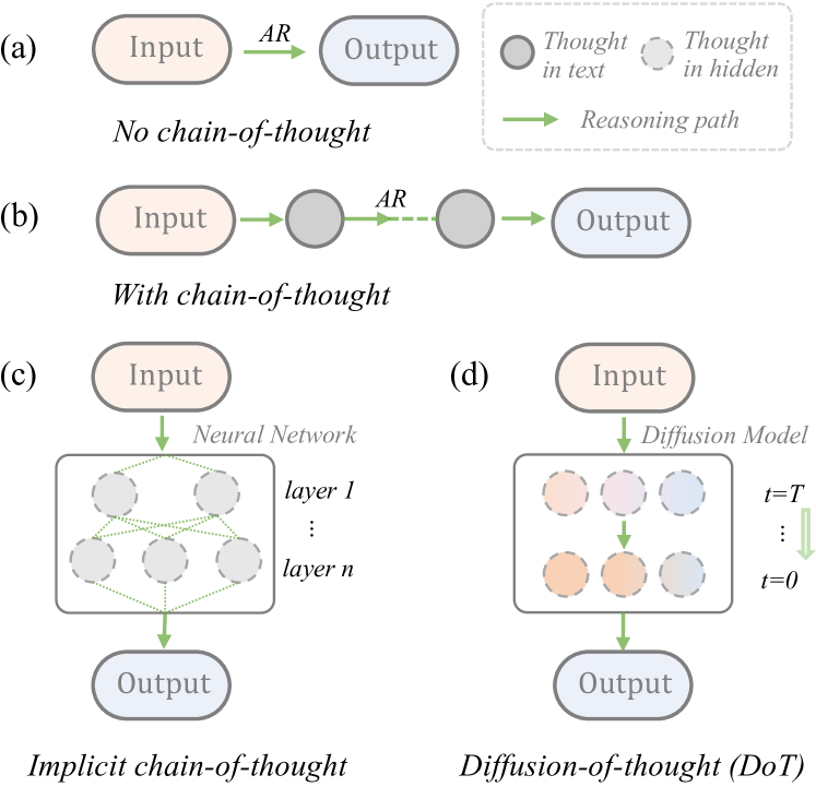
Figure 1: Schematic illustration of different approaches for problem solving tasks. (a) No CoT and (b) CoT generate left-to-right text tokens by prompting autoregressive (AR) language model. (c) Implicit CoT replaces horizontal reasoning (CoT) with vertical reasoning from shallow layer to deep layer (Deng et al., 2023). (d) DoT generates reasoning path along with the diffusion timesteps. Detailed formulations can be found in §3.1.

Large language models (LLMs) have had a profound impact on the entire field of artificial intelligence (OpenAI, 2023; Touvron et al., 2023), transforming our approach to addressing classical problems in natural language processing and machine learning. Among the most notable aspects of LLMs is their remarkable reasoning ability, which many researchers consider to be a representative emergent capability brought about by LLMs (Wei et al., 2022a). Chain of thought prompting (CoT; Wei et al. 2022b), which generates a series of intermediate reasoning steps in autoregressive (AR) way, has emerged as a central technique to support complex reasoning processes in LLMs.

Recently, diffusion models have attracted interest in text processing (Li et al., 2022; Zheng et al., 2023; Zou et al., 2023) as a result of success in the vision domain and distinctive modeling strengths over autoregressive models (Lin et al., 2021), offering potential benefits including global planning ability (Zhang et al., 2023b; Ye et al., 2023b) and self correction (Hoogeboom et al., 2021). As part of the research community effort, pre-trained diffusion language models such as Plaid (Gulrajani & Hashimoto, 2023) have shown significant progress in text generation capabilities. Although they have not yet attained the scale and capabilities of existing proprietary autoregressive LLMs like GPT-4 (OpenAI, 2023), these models have demonstrated performance on par with GPT-2 (Brown et al., 2020). Meanwhile, Gulrajani & Hashimoto (2023) highlights the scaling law (Kaplan et al., 2020) in diffusion language models and Ye et al. (2023b) exhibits that diffusion models can handle complex tasks upon instruction-tuning and scaling. As a result, it becomes pertinent to explore the following question: can diffusion language models also leverage the CoT-style technique to gain enhanced complex reasoning abilities?

This work presents a preliminary study on this question. We propose Diffusion of Thought (DoT), an inherent chain-of-thought method tailored for diffusion models. In essence, DoT progressively updates a sequence of latent variables representing thoughts in the hidden space, allowing reasoning steps to diffuse over time. From a methodological standpoint, DoT shares similarities with the recently proposed Implicit CoT approach (Deng et al., 2023), where the latter learns thoughts in hidden states across transformer layers to improve the time efficiency of autoregressive CoT generation. A schematic illustration of CoT, Implicit CoT, and DoT can be found in Figure 1. In practice, DoT iteratively imposes Gaussian noise on data points at each diffusion timestep $t$, where $t$ runs from $t=0$ (least noisy) to $t=T$ (most noisy), and then a denoising model is trained to recover clean data from the noisy one. To condition on complex queries, instead of using gradient-based classifier guidance (Li et al., 2022; Gulrajani & Hashimoto, 2023), DoT trains and samples from the denoising model using the classifier-free guidance proposed in Gong et al. (2023b), to provide more reliable controlling signals on exact tokens.

Furthermore, thanks to the intrinsic self-correcting capability of the diffusion model, DoT can more robustly rectify errors originating from prior or current reasoning steps. This feature offers a fresh angle on the issue of error accumulation (Lanham et al., 2023; Huang et al., 2023) inherent in autoregressive models. Finally, DoT provides more flexibility in trading off computation (reasoning time) and performance, as more complex problems may necessitate increased computation in reasoning (Banino et al., 2021; Wei et al., 2022b).

The main contributions of our paper are threefold:

1. We first introduce the CoT technique on diffusion (DoT), and showcase its advantages in digit multiplication tasks when compared to autoregressive CoT and Implicit CoT. DoT achieves more than $27\times$ speed-up compared to baselines with similar performance (§4.2).

2. We further adapt DoT to the currently largest pre-trained text diffusion model Plaid 1B and introduce two sampling algorithms to improve its training efficacy. DoT exhibits a promising performance similar to GPT-2 with CoT on grade school math problems, showing sparks of complex reasoning ability in text diffusion models (§4.3).

3. Our analysis demonstrates the flexibility of DoT in the trade-off between reasoning time and performance (§4.4), and showcases DoT’s self-correction capability (§4.5). We also find that self-consistency decoding can further improve DoT and its multi-pass variant (§4.6).

Although it is challenging for current pre-trained diffusion language models to directly compete with LLMs that are hundreds of times larger in parameter size, our study emphasizes the possibility of their complex reasoning abilities and highlights the substantial potential in developing LLMs that go beyond the autoregressive paradigm. We release all the codes at https://github.com/HKUNLP/diffusion-of-thoughts.

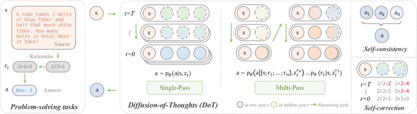
Figure 2: Demonstration of DoT pipeline. DoT diffuses all possible thoughts across diffusion timestep $t$. Multi-pass DoT disentangles each rationale and introduces causal information. The stacked circles stand for the marginalization over other potential reasoning paths, which is implicitly carried out during the training of diffusion models.

2 Preliminaries

This section introduces key concepts and notations in diffusion models for text generation. Detailed formulations and derivations are provided in Appendix A.

2.1 Diffusion in Seq2Seq Generation

In the context of text generation, continuous diffusion models (Li et al., 2022) based on DDPM (Ho et al., 2020) map the discrete text $\mathbf{w}$ into a continuous space through an embedding function $\textsc{Emb}(\mathbf{w})$, and its inverse operation is called rounding. For sequence-to-sequence (seq2seq) generation, which involves a pair of sequences $\mathbf{w}^{x}$ and $\mathbf{w}^{y}$, the model learns a unified feature space for $\textsc{Emb}(\mathbf{w})$. Different from separating the feeding of $\mathbf{w}^{x}$ and $\mathbf{w}^{y}$ in encoder-decoder architectures, DiffuSeq (Gong et al., 2023b) treats these two sequences as a single one $\mathbf{w}^{z}=\mathbf{w}^{[x;y]}$ and uses a left-aligned mask during the forward and reverse diffusion process to distinguish them. Denote $\mathbf{z}_{t}=[\mathbf{x}_{t};\mathbf{y}_{t}]$ with mask $[\mathbf{0};\mathbf{1}]$, where vector presentation $\mathbf{x}_{t}$ and $\mathbf{y}_{t}$ represent parts of $\mathbf{z}_{t}$ that belong to $\mathbf{w}^{x}$ and $\mathbf{w}^{y}$, respectively. For each forward step, the Markov transition is defined as:

$$q(\mathbf{z}_{t}|\mathbf{z}_{t-1})=\mathcal{N}(\sqrt{1-\beta_{t}}\mathbf{z}_{t-1},{\beta}_{t}\mathbf{I}),$$ (1)

with $t=1,2,...,T$ and $\{\beta_{t}\in(0,1)\}_{t=1}^{T}$ representing the variance schedule. Larger $t$ corresponds to noisier data. An additional transition ${q_{\phi}}(\mathbf{z}_{0}|\mathbf{w})=\mathcal{N}(\textsc{Emb}(\mathbf{w}),\beta_{0}\mathbf{I})$ presents the embedding function. In the forward chain, noise is gradually injected into last step’s hidden state $\mathbf{z}_{t-1}$ to obtain $\mathbf{z}_{t}$. Through accumulation, $\mathbf{z}_{t}$ can be reparameterized by $\mathbf{z}_{0}$ directly:

$$q(\mathbf{z}_{t}|\mathbf{z}_{0})=\mathcal{N}(\sqrt{\bar{\alpha}_{t}}\mathbf{z}_{0},(1-\bar{\alpha}_{t})\mathbf{I}),$$ (2)

where $\alpha_{t}=1-\beta_{t}$ and $\bar{\alpha}_{t}=\prod_{i=1}^{t}\alpha_{i}$. Unlike traditional diffusion models that corrupt the entire $\mathbf{z}_{t}$ (both $\mathbf{x}_{t}$ and $\mathbf{y}_{t}$) without distinction, DiffuSeq only adds noise to those entries with the mask value of 1 (e.g., $\mathbf{y}_{t}$). This modification, termed partial noising, tailors diffusion models for conditional language generation.

2.2 Pre-trained Diffusion Language Models

Plaid 1B (Gulrajani & Hashimoto, 2023) is a diffusion language model trained from scratch on 314B tokens from OpenWebText2 (Gao et al., 2021), with $1024$ context size. It is currently the largest scale diffusion language model with 1.3B parameters. It adopts the formulation of Variational Diffusion Models (VDM) (Kingma et al., 2021), with a natural fit for likelihood-based training, compared to DDPM. The implementation of $\textsc{Emb}(\mathbf{w})$ is the same with §2.1. The diffusion process is defined in continuous time space in that for any $t\in[0,1]$, the distribution of latent $\mathbf{z}_{t}$ conditioned on $\mathbf{z}_{0}$ is given by:

$$q(\mathbf{z}_{t}|\mathbf{z}_{0})=\mathcal{N}(\alpha_{t}\mathbf{z}_{0},\sigma_{t}^{2}\mathbf{I}).$$ (3)

Note that $\alpha_{t}$ here shares different scheduled value in §2.1. The variance-preserving special case gives $\alpha_{t}=\sqrt{1-\sigma_{t}^{2}}$ in VDM. The physical meaning of them is defined by the signal-to-noise ratio: $\text{SNR}(t)=\alpha_{t}^{2}/\sigma_{t}^{2}$. One of the crucial differences in VDM is that the noise schedule $\alpha_{t}$ and $\sigma_{t}^{2}$, which specify how much noise to add at each time in the diffusion process, are parameterized as a scalar-to-scalar neural network $\boldsymbol{\eta}$ that satisfies $\sigma_{t}^{2}=\operatorname{sigmoid}\left(\gamma_{\boldsymbol{\eta}}(t)\right)$ and $\alpha_{t}^{2}=\operatorname{sigmoid}\left(-\gamma_{\boldsymbol{\eta}}(t)\right)$, instead of a predefined function. The distributions $q(\mathbf{z}_{t}|\mathbf{z}_{s})$ for any $t>s$ are also Gaussian:

$$q(\mathbf{z}_{t}|\mathbf{z}_{s})=\mathcal{N}(\alpha_{t\mid s}\mathbf{z}_{s},\sigma_{t\mid s}^{2}\mathbf{I}),$$ (4)

where $\alpha_{t\mid s}=\alpha_{t}/\alpha_{s}$ and $\sigma_{t\mid s}^{2}=\sigma_{t}^{2}-\alpha_{t\mid s}^{2}\sigma_{s}^{2}$. It is highlighted in Gulrajani & Hashimoto (2023) that Plaid 1B fits the scaling law  (Kaplan et al., 2020) observed in autoregressive models and Plaid 1B can generate fluent samples in both unconditional and zero-shot conditional settings. The conditional generation relies on gradient-based token guidance similar to  Li et al. (2022).

3 Diffusion-of-Thoughts

In this section, we begin with an overview of our method and its relationship with other paradigms (§3.1). We then introduce Diffusion-of-Thoughts (DoT; §3.2) as well as its multi-pass variant (DoT${}^{\text{MP}}$; §3.3), as illustrated in Figure 2. Following this, we outline the implementation of our training (§3.4) and inference (§3.5) protocols.

3.1 Overview

Without loss of generality, we use the mathematical problem-solving task as our running example. A problem statement and its correct answer are denoted as $\mathbf{s}$ and $\mathbf{a}$, respectively. We employ a language model with parameters $\theta$, represented as $p_{\theta}^{\textit{LM}}$, to find the solution for each problem. For regular usage of language models without Chain-of-Thoughts (CoT), the final answer $\mathbf{a}$ is generated directly as $\mathbf{a}\sim p_{\theta}^{\textit{LM}}(\mathbf{a}|\mathbf{s})$. The CoT approach introduces meaningful intermediate steps or rationales $\mathbf{r}_{1},\dots,\mathbf{r}_{n}$ for language models to bridge $\mathbf{s}$ and $\mathbf{a}$, resulting in the output $\mathbf{a}\sim p_{\theta}^{\textit{LM}}(\mathbf{a}|\mathbf{s},\mathbf{r}_{1\dots n})$. For implicit CoT (Deng et al., 2023), the hidden representations of rationales $\mathbf{z}_{1},\dots,\mathbf{z}_{n}$ are distilled into transformer layers, leading to $\mathbf{a}\sim p_{\theta}^{\textit{iCoT}}(\mathbf{a}|\mathbf{s},\mathbf{z}_{1\dots n})$. Similarly but differently, for DoT, these representations are distributed over diffusion timestep $t$ as $\mathbf{a}\sim p_{\theta}^{\textit{DoT}}(\mathbf{a}|\mathbf{s},\mathbf{z}_{t})$, where $\mathbf{z}_{t}$ corresponds exactly to the noised data in diffusion models.

3.2 DoT

Inspired by the success of diffusion models for text generation, we are eager to explore their reasoning ability in particular tasks and potential advantages over autoregressive models. We begin by observing the default gradient-based token guidance in Plaid (Gulrajani & Hashimoto, 2023) fails to do accurate conditioning as the model cannot exactly recover each conditioning token. This is vital, especially in mathematical reasoning, as it is expected to perform reasoning based on exact tokens (e.g., numbers) in the problem statement, rather than more compact gradient signals. For this, we adopt DiffuSeq-style (Gong et al., 2023a) classifier-free conditioning during the fine-tuning of Plaid. This yields a prototype of DoT, where all rationales are generated by the backward diffusion process in one pass and all the conditional tokens are fixed as still. Specifically, the problem context is concatenated with the rationales (chain-of-thought reasoning path) $\mathbf{z}_{0}=\textsc{Emb}([\mathbf{s};\mathbf{r}_{1\dots n}])$ during training and sampling, and the partial noise is only imposed to the rationale part in $\mathbf{z}_{t}$, keeping $\mathbf{s}$ anchored as the condition. This fine-tuning style is consistent with §2.1.

DoT benefits from the intrinsic self-correcting capability of the diffusion models through the multi-step denoising process. To further improve self-correcting ability, we design a scheduled sampling mechanism building upon previous practices (Bengio et al., 2015; Deng et al., 2022) such that self-generated error thoughts are exposed and corrected during the training stage. Formally, for any continuous timesteps $s$, $t$, $u$ that satisfy $0<s<t<u<1$, $\mathbf{z}_{t}$ is sampled from $q\left(\mathbf{z}_{t}\mid\mathbf{z}_{0}\right)=\mathcal{N}\left(\alpha_{t}\mathbf{z}_{0},\sigma_{t}^{2}\mathbf{I}\right)$ in the training stage while during inference it is sampled from $q(\mathbf{z}_{t}\mid f_{\theta}\left(\mathbf{z}_{u};u\right))$ instead, where $f_{{\theta}}$ is a denoiser neural network that reparameterizes $\mathbb{E}_{q}[\mathbf{z}_{0}|\mathbf{z}_{t}]$. The presence of such exposure bias may impede the model’s ability to recover from erroneous thoughts during the generation process as the model $f_{{\theta}}$ has only been trained on corruptions $\mathbf{z}_{t}$ diffused from oracle data. To mitigate this problem, we mimic the inference stage with probability $\epsilon_{i}$ during training depending on the current training step $i$, and $\epsilon_{i}$ linearly decays from 1 to $\epsilon_{min}$. Specifically, for time-step $t$, we randomly sample a former continuous time-step $u\in(t,1]$, obtain $\mathbf{z}_{u}$ by Eq. (3), and perform a model forward pass to get a predicted $\hat{\mathbf{z}}_{0}=f_{\theta}\left(\mathbf{z}_{u};u\right))$. $\mathbf{z}_{t}$ is then sampled from $q(\mathbf{z}_{t}\mid\hat{\mathbf{z}}_{0})$ to replace the regular one in loss calculation. Compared with scheduled sampling for autoregressive models, such a mechanism in DoT helps the model to recover from errors considering global information instead of relying on the left-side tokens.

3.3 Multi-pass DoT

We further propose a multi-pass (MP) variant of DoT, denoted as DoT${}^{\text{MP}}$, which generates rationales in a thought-by-thought paradigm. This method disentangles the generation of multiple rationales and introduces casual inductive bias such that later rationale can be guided by stronger condition signals of prior rationales during the generation. Specifically, in the first pass, we generate the first rationale by $\mathbf{r}_{1}\sim p_{\theta}^{\textit{DoT}}(\mathbf{r}_{1}|\mathbf{s},\mathbf{z}^{r_{1}}_{t})$, where $\mathbf{z}^{r_{1}}_{t}$ is the noised vector representation of $\mathbf{r}_{1}$ in diffusion model. Then $\mathbf{r}_{1}$ is connected to $\mathbf{s}$ as the condition $[\mathbf{s};\mathbf{r}_{1}]$ to get $\mathbf{r}_{2}\sim p_{\theta}^{\textit{DoT}}(\mathbf{r}_{2}|[\mathbf{s};\mathbf{r}_{1}],\mathbf{z}^{r_{2}}_{t})$, and then we have $[\mathbf{s};\mathbf{r}_{1};\mathbf{r}_{2}]$. Through multiple iterations, we can get the final answer: $\mathbf{a}\sim p_{\theta}^{\textit{DoT}}(\mathbf{a}|[\mathbf{s};\mathbf{r}_{1};...;\mathbf{r}_{n}],\mathbf{z}^{r_{n}}_{t})$.

Multi-pass DoT shares a similar spirit of auto-regressive decoding, but it differs in that tokens in each thought are generated in parallel through the diffusion model, allowing hidden representations to diffuse within each thought. Additionally, we also implement glancing sampling (Qian et al., 2021) to improve the self-correction ability. We select a small portion of $t$ from $T$ with the ratio $\gamma$ to incorporate the condition of the consecutive rationale as a glance when predicting the current rationale. For instance, the previous sequence $\mathbf{z}_{0}=\textsc{Emb}([\mathbf{s};\mathbf{r}_{1}])$ will be modified to $\mathbf{z}_{0}=\textsc{Emb}([\mathbf{s};\mathbf{r}_{1};\mathbf{r}_{2}])$, with the partial noise being applied to $[\mathbf{r}_{1};\mathbf{r}_{2}]$ rather than just the last rationale $\mathbf{r}_{2}$. Therefore, the model learns to recover from errors in $\mathbf{r}_{1}$ when predicting $\mathbf{r}_{2}$. The new $\mathbf{z}_{0}$ will be reparameterized into $\mathbf{z}_{t}$ as before and other procedures are the same as in DoT.

3.4 Model Training

Given a set of training data for problem-solving tasks of size $D$: $\{\mathbf{s}^{i},\mathbf{r}^{i}_{1\dots n},\mathbf{a}^{i}\}_{i\in D}$, we have two training settings for DoT models: one is training from scratch, while the other involves DoT models with fine-tuning the pre-trained Plaid 1B model. To train from scratch, we follow §2.1 to train a denoiser model $f_{\theta}(\mathbf{z}_{t},t)$ to approximate the least noisy data ($t=0$). To fine-tune Plaid 1B, we follow the diffusion formulation in §3.2. In both training settings, we share the same training objective to minimize the variational lower bound $\mathcal{L}_{\text{VLB}}(\mathbf{w}^{z})$:

$$\mathbb{E}_{q({\mathbf{z}_{0}}\mid\mathbf{w}^{z})}\Bigg{[}\underbrace{\log\frac{q(\mathbf{z}_{T}|\mathbf{w}^{z})}{p_{\theta}(\mathbf{z}_{T})}}_{\text{Prior loss}}+\underbrace{\textstyle\mathcal{L}_{\text{VLB}}(\mathbf{z}_{0})}_{\text{Diffusion loss}}\underbrace{-\log p_{\theta}(\mathbf{w}^{z}|\mathbf{z}_{0})}_{\text{Rounding loss}}\Bigg{]},$$ (5)

where $p_{\theta}$ models the reverse denoising process and the diffusion loss sums up the KL divergence of each time step $t$. Following the pre-training stage of Plaid, we adopt Monte Carlo estimation to compute the loss for optimization, and please refer to Appendix A for detailed formulation.

3.5 Inference

One of the significant advantages of diffusion models is their inference flexibility. We follow Gong et al. (2023a) to use DPM-solver (Lu et al., 2022b, a) to accelerate generation during inference. By adjusting the diffusion timesteps $T$ during sampling, it becomes flexible to control the trade-off between generation time and quality. Sharing a similar idea of MBR (Koehn, 2004), self-consistency (Wang et al., 2022) boosts the performance of CoT significantly by generating and aggregating multiple samples. In the context of diffusion models, we can also expect its potential improvement using self-consistency, thanks to their ability to naturally produce diverse responses. After sampling $m$ times to obtain multiple reasoning pathways $(\mathbf{r}_{i;1...n},\mathbf{a}_{i})$ from DoT, self-consistency involves marginalizing over $\mathbf{r}_{i;1...n}$ by taking a majority vote over $\mathbf{a}_{i}$, i.e., $\arg\max_{\mathbf{a}}\sum_{i=1}^{m}\mathbbm{1}(\mathbf{a}_{i}=a)$. We consider this as the most “consistent” answer among the candidate set of $m$ answers. Intuitively, it is also possible to apply Tree-of-Thoughts (Yao et al., 2023) to the multi-pass variants of DoT, and we leave it to future work.

4 Experiments

We conduct experiments on both simple multi-digit multiplication and complex grade school math problems, to explore the reasoning paradigm in diffusion models.

4.1 Experimental Setup

Datasets and Metrics.

Building on Deng et al. (2023), we employ the four-digit ($4\times 4$) and five-digit ($5\times 5$) multiplication problems from the BIG-bench benchmark (Suzgun et al., 2023), known to be challenging for LLMs to solve without CoT. As a more complex task, grade school math problems require both language understanding and mathematical reasoning. We adopt the widely-used GSM8K dataset (Cobbe et al., 2021), using the augmented training data from Deng et al. (2023) and keep all original test sets unchanged. The statistics are listed in Appendix 4. For both datasets, we use accuracy (Acc.) to measure the exact match accuracy of predicting the final answer, and throughput (Thr.) to measure the number of samples processed per second (it/s) during inference with a batch size of $1$.

Table 1: Preliminary results on digit multiplication tasks. Acc. is for accuracy, and Thr. for throughput measuring the number of processed instances per second (it/s). ^† denotes that the results are taken from the Implicit CoT paper (Deng et al., 2023), and have been validated reproducible by us.

Models	$4\times 4$		$5\times 5$
	Acc. $\uparrow$	Thr. $\uparrow$	Acc. $\uparrow$	Thr. $\uparrow$
	(%)	(it/s)	(%)	(it/s)
Transformer-scratch	3.9	2.2	1.0	1.5
GPT-2
CoT-fewshot-large	0.0	0.3	0.0	0.3
No CoT-finetune-large†	33.6	4.8	0.9	4.0
CoT-finetune-small†	100	2.3	100	1.5
CoT-finetune-medium†	100	1.2	100	0.8
CoT-finetune-large†	100	0.8	99.3	0.6
ChatGPT
CoT-fewshot	43.5	-	4.5	-
No CoT-fewshot	2.4	-	0.0	-
Implicit CoT†
GPT2-small	96.6	8.9	9.5	7.9
GPT2-medium	96.1	4.8	96.4	4.3
Diffusion-of-Thoughts (DoT)
DoT-scratch	100	62.5	100	61.8
DoT${}^{\text{MP}}$-scratch	100	11.8	100	9.5

Base Models.

When training from scratch, we follow DiffuSeq to use a 12-layer Transformer (Vaswani et al., 2017) encoder. We also apply Plaid 1B as the base model for further fine-tuning, which is presently the largest pre-trained diffusion model and is comparable to GPT-2 small in perplexity. Our primary focus on digit multiplication tasks involves DoT trained from scratch, while for GSM8K we explore more on DoT fine-tuned from Plaid 1B.

Baselines.

We use GPT-2 (Brown et al., 2020) at various scales as baselines, known as conventional autoregressive language models. We explore several variants, such as prompting LMs using CoT few-shot demonstrations, or fine-tuning with CoT/No CoT training data. Additionally, we consider training a 12-layer seq2seq Transformers from scratch, and the strong commercial LLM ChatGPT gpt-3.5-turbo-1106 as baselines. In the few-shot setting, we use $5$-shot. Another important baseline is Implicit CoT (Deng et al., 2023), which distills thoughts into transformer layers to accelerate CoT reasoning.

Implementation Details.

During tokenization, we treat all the digits as individual tokens. We conduct all the experiments on NVIDIA V100-32G GPUs in half precision (fp16), and we use 8 GPUs for training and sampling. During training, we set $\epsilon_{min}$ to be $0.95$ as we find decreasing the probability of oracle demonstration hinders model training. We choose glance sampling $\gamma=0.01$ and self-consistency $m=20$. Following Plaid, we also adopt self-conditioning (Chen et al., 2022) during training. During inference, we set both the temperature of the score and output logit to 0.5 to sharpen the predicted output distribution while maintaining the ability to generate diverse samples. By default, we set the sampling timesteps $T$ to be 64. Other details can be found in Appendix B.4.

4.2 Results on Digit Multiplication

We first train DoT from scratch for digit multiplication tasks as the preliminary investigation, as shown in Table 1. We observe that neither ChatGPT nor the distilled Implicit CoT model can reach 100% accuracy. GPT-2 can be fine-tuned to achieve high accuracy but sacrifices throughput during CoT. Interestingly, DoT trained from scratch can attain 100% accuracy while maintaining significant throughput with diffusion sampling steps set at $1$. This preliminary finding indicates that DoT performs well in modeling exact math computation, and also benefits from its computational efficiency. We continue training DoT in GSM8K from scratch, but we are only able to achieve an accuracy of $5.61\%$ (Appendix B.5), which is lower than the fine-tuned version of GPT-2. We believe that this is mainly due to the absence of pre-trained natural language understanding capability when training DoT from scratch. This is why we start to explore further by fine-tuning with pre-trained diffusion models.

Table 2: The main results on GSM8K-Aug. Acc. is for accuracy, and Thr. for throughput. ^† denotes that the results are taken from the Implicit CoT paper (Deng et al., 2023).

Models	Acc. (%) $\uparrow$	Thr. (it/s) $\uparrow$
Transformer-scratch	2.27	1.9
GPT-2
CoT-fewshot-large	1.70	0.3
No CoT-finetune-large†	12.7	9.1
CoT-finetune-small†	40.7	2.0
CoT-finetune-small (reproduce)	39.0	2.4
+ self-consistency	40.6	-
ChatGPT
CoT-fewshot	62.5	-
No CoT-fewshot	28.2	-
Implicit CoT†
GPT2-small	20.0	16.4
GPT2-medium	21.9	8.7
Pretrained Diffusion Model (Plaid 1B)
No DoT-finetune	12.4	0.3
DoT-finetune ($T$=8)	28.7	2.3
DoT-finetune	32.6	0.3
+ self-consistency	36.3	-
DoT${}^{\text{MP}}$-finetune ($T$=4)	36.2	1.4
DoT${}^{\text{MP}}$-finetune	37.7	0.1
+ self-consistency	40.3	-

4.3 Results on Grade School Math

We further extend DoT to a pre-trained diffusion language model Plaid 1B (Gulrajani & Hashimoto, 2023) and evaluate on a more complex reasoning task, i.e., GSM8K. In Table 2, both autoregressive models and diffusion models show significantly improved performance when fine-tuned with CoT or DoT, compared to not using CoT/DoT. This suggests that increased computation (reasoning time) brings substantial benefits. DoT, which shares a similar formulation to Implicit CoT, yet demonstrates notably enhanced reasoning ability than it, comparable to the GPT-2 fine-tuned CoT model. Multi-pass DoT, with casual bias, performs slightly better than single-pass one, while the latter is more efficient. Additionally, self-consistency yields more noticeable improvements in DoT models than in GPT models. Further interesting analyses are in the subsequent subsections.

When fine-tuning Plaid 1B, we explore several alternatives and conduct an ablation study as in Table 3. As discussed above, continuing pre-training Plaid 1B using the GSM8K-augmented dataset and performing reasoning with gradient-based conditioning is not a good choice for fine-tuning diffusion LMs on downstream tasks, because reasoning tasks require more specific guidance. Moreover, the ablation of two sampling strategies proposed in §3.2 and §3.3 showcases their effectiveness. This provides evidence that better denoising models are trained using our training sampling strategies, allowing DoT models to self-correct more effectively during inference. Further analysis is listed in §4.5.

Table 3: The ablation study of DoT on GSM8K-Aug. $*$ denotes the results of directly applying the same loss function as the pre-training stage of Plaid to the fine-tuning stage.

Models	Acc. (%) $\uparrow$
Continue pre-training∗	0.5
DoT-finetune	32.6
(-) scheduled sampling	31.2
DoT${}^{\text{MP}}$-finetune	37.7
(-) glancing sampling	35.5

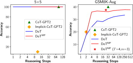
Figure 3: Accuracy over reasoning steps using various methods. We measure the reasoning steps as the average number of calling the model forward function for instances from the test set. DoT provides a flexible way to balance accuracy and efficiency through the reasoning steps. $T$ refers to diffusion timesteps during inference, and $m$ refers to the number of samples in self-consistency.

Table 4: Cases that show the predictions of DoT at each time-step $t$ with $T$=8 on the GSM8K test set. The incorrect thoughts are marked in bold red and we omit some correct predictions when $t<4/8$. The difficulty level of the questions increases from left to right.

4.4 Reasonability-efficiency Trade-off

The community has devoted substantial efforts to improve the reasoning capabilities of left-to-right language models, such as refining instructions (Kojima et al., 2022; Zhou et al., 2022, inter alia), finding better demonstrations (Fu et al., 2022; Wu et al., 2022; Ye et al., 2023a, inter alia), and designing elaborate decoding algorithm (Shinn et al., 2023; Xie et al., 2023; Yao et al., 2023, inter alia). Non-autoregressive diffusion models naturally provide another simple way to enhance reasoning by allocating more timesteps during inference, albeit at the expense of efficiency. We show such efficiency trade-off in Figure 3, where we measure the reasoning steps as the average number of calling the model forward function for all the instances from the test set. For CoT and Implicit CoT baselines, we treat reasoning steps as the average number of output tokens for all the test instances. The average predicted thoughts of DoT${}^{\text{MP}}$ are 6 and 1.98 on 5$\times$5 and GSM8K datasets, respectively. Therefore, DoT${}^{\text{MP}}$ needs around 5 and 1 times more reasoning steps than DoT under the same denoising steps for 5$\times$5 and GSM8K datasets.

Given a small budget of reasoning steps (e.g., 1) on simpler tasks such as 5$\times$5, both DoT and DoT${}^{\text{MP}}$ already have an accuracy of 100%, and no more reasoning steps are needed. For such cases of simple tasks, only a little computation cost is required for our method. In comparison, CoT and Implicit CoT with the autoregressive model are hard to be more efficient given their nature of token-by-token prediction. For complex tasks such as GSM8K, we find both DoT and DoT${}^{\text{MP}}$ produce similar results as Implicit CoT with only 2 reasoning steps, and their performance can continuously improve by allowing more reasoning steps. This indicates DoT can be efficient if we can sacrifice performance in certain scenarios. Overall, with DoT, we can flexibly control the trade-off between efficiency and performance for tasks with different difficulty levels.

4.5 Self-correction in DoT

In this section, we provide several cases in Table 4 to show the self-correction ability of DoT, which acts as a distinct difference between diffusion models and autoregressive models. In the first case, we can see the model figures out all the correct thoughts together with only a single reasoning step (i.e., a single calling of the model forward function), and obtains the correct final answer in the second step. This mirrors how humans think in both fast and slow modes (Kahneman, 2011). In the second case where the problem is slightly harder, the model cannot give concrete thoughts in the first step but can still produce the correct answer through the later “slow” thinking process. We can see the solution framework, roughly outlining how the task will be carried out, is established at the very beginning, and then the subsequent work is for refining and improving, which is also similar to how human performs a complex task. Interestingly, in DoT, the correct thoughts may not appear in a left-to-right paradigm as in the traditional chain-of-thought process. The third case serves as compelling evidence to illustrate this distinctive nature of diffusion-of-thought and how it diverges from the chain-of-thought approach. In step 4 the model has a wrong intermediate thought <<2*3=4>> with the latter thoughts and final answer computed correctly first. In the next step, the error in the wrong intermediate thought is fixed, which suggests both prior and latter thoughts can help in the prediction of the current thought. Furthermore, from these three cases, we observed that the model tends to maintain its prediction after it considers the answer to be complete. This suggests we can further enhance the inference efficiency by incorporating mechanisms such as early exit (Graves, 2016), and easier tasks can get earlier exits as observed in Table 4.

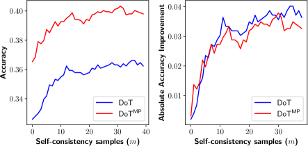
Figure 4: (Left) Accuracy versus samples per instance for the self-consistency method on the GSM8K dataset. (Right) Absolute accuracy improvement under different samples per instance compared with the baseline of removing self-consistency.

4.6 Self-consistency in DoT

Figure 4 shows the efficacy of the self-consistency mechanism for DoT and its variant. We can see self-consistency improves both DoT and DoT${}^{\text{MP}}$, which is in line with the effectiveness of self-consistency for auto-regressive models (Wang et al., 2022). From the right subfigure, we can see by generating 10 samples for each instance, we can improve both DoT and DoT${}^{\text{MP}}$ by around 3%. This benefits from the diversity generation in DoT. We can observe that DoT can generate diverse reasoning paths, such as <<3*3=9>><<9*60=540>> and <<3*60=180>><<180*3=540>> for the same question, providing cross validation when selecting the most “consistent” answer. Note that different from autoregressive models, where diversity usually relies on decoding algorithms (Fan et al., 2018; Holtzman et al., 2020), the natural advantage of the diffusion models is to generate different sentences with different initial random Gaussian noises.

5 Related Work

5.1 Diffusion Models for Text

Building upon advancements in diffusion models for image generation (Ho et al., 2020; Song et al., 2021), Diffusion-LM (Li et al., 2022) and DiffuSeq (Gong et al., 2023b) achieve constrained and conditional generation respectively, by employing an embedding function to transform discrete text into a continuous space. Besides, discrete diffusion models (Ho et al., 2020; Austin et al., 2021) directly introduce discrete noise to accommodate the discrete nature of texts, demonstrating significant potential (Zheng et al., 2023; Lou et al., 2023). Numerous studies have shown that diffusion models can efficiently generate diverse texts (Gong et al., 2023a; Gao et al., 2022). Additionally, diffusion models have shown competitive performance in various sequence-to-sequence NLP tasks, including machine translation (Yuan et al., 2022; Ye et al., 2023c), summarization (Zhang et al., 2023a), code generation (Singh et al., 2023), and style transfer (Horvitz et al., 2023).

5.2 Pre-train and Fine-tune Diffusion LMs

The pre-training and fine-tuning paradigm, while a familiar concept in NLP before the era of prompting methods (Liu et al., 2023), remains relatively under-explored for diffusion language models. Prior efforts involve initializing diffusion models with pre-trained models such as BERT (He et al., 2022) and RoBERTa (Zhou et al., 2023). Furthermore, Ye et al. (2023b) explored instruction tuning upon masked language models. GENIE (Lin et al., 2023) adopts paragraph denoising to train encoder-decoder models, proving beneficial for downstream summarization tasks. Plaid 1B (Gulrajani & Hashimoto, 2023) and SEDD (Lou et al., 2023) are pioneers to pre-train diffusion language models from scratch, attaining comparative or better perplexity scores over GPT-2 (Brown et al., 2020). To the best of our knowledge, we are the first to explore the fine-tuning of a pre-trained diffusion language model.

5.3 Chain-of-Thought Reasoning

Large language models usually excel in performing system-1 (Stanovich & West, 2000) tasks that are processed quickly and intuitively by humans but struggle in system-2 tasks, which require deliberate thinking (Brown et al., 2020; Wei et al., 2022b; Suzgun et al., 2022). The chain-of-thought reasoning paradigm (Nye et al., 2021; Wei et al., 2022b; Kojima et al., 2022) has been widely employed to elicit reasoning abilities, which can be further improved with various techniques. For instance, self-consistency (Wang et al., 2022) samples a diverse set of reasoning paths and selects the most consistent answer, while tree-of-thought (Yao et al., 2023) achieves different reasoning paths by tree search. Despite these advancements, errors introduced in intermediate CoT steps can lead to inaccurate answers (Lanham et al., 2023), posing difficulties in self-correction (Huang et al., 2023). Moreover, there are concerns about the inefficiency of CoT, as highlighted by recent studies (Deng et al., 2023). While diffusion models show potential for reasoning tasks (Ye et al., 2023b), the exploration of their CoT reasoning abilities remains limited in the literature.

6 Conclusion and Limitation

In this work, we propose diffusion-of-thought (DoT), integrating CoT reasoning with continuous diffusion models. We thoroughly evaluate DoT on representative reasoning tasks in various aspects, including their flexible control of reasoning efficiency, self-correction capability, and the ability to generate diverse reasoning paths. Considering pre-trained diffusion models are still in their early stages, particularly in terms of model scales compared to the more extensively studied autoregressive language models, our study presents an initial exploration into the reasoning ability of current diffusion language models. A notable limitation of DoT is its requirement for additional training to achieve accurate reasoning. With more powerful pre-trained diffusion models, we anticipate DoT can attain comparative or better generalization capabilities of auto-regressive language models while removing the need for specialized training. Besides, the diffusion training techniques employed in this work are general and applicable to other tasks beyond mathematical reasoning. Extending our training recipes of diffusion language models to further scaled setups, such as multi-task instruction tuning, is an interesting avenue for future research.

Impact Statement

This paper presents work whose goal is to advance the field of Machine Learning. There are many potential societal consequences of our work, none of which we feel must be specifically highlighted here.

Appendix A Derivations

A.1 Seq2Seq Modeling in DiffuSeq

To implement the diffusion model in seq2seq generation, we inherit the design from DiffuSeq (Gong et al., 2023a), which systematically defines the $forward~{}noising$ process and $reverse~{}denoising$ process on latent continuous space z as two major components of the model.

Latent space configuration z.

Following Li et al. (2022), z is constructed from an embedding function $\textsc{Emb}(\mathbf{w^{z}})$, which takes the discrete text $\textbf{w}^{z}$ as input. Particulatly, in Diffuseq (Gong et al., 2023a), $\textbf{w}^{z}$ contains $\mathbf{w}^{x}$ and $\mathbf{w}^{y}$ where $\mathbf{w}^{x}$ is the source sequence and $\mathbf{w}^{y}$ is the target sequence. The relationship is defined as $\mathbf{w}^{z}=\mathbf{w}^{[x;y]}$. They denote $\mathbf{z}_{t}=\mathbf{x}_{t}\oplus\mathbf{y}_{t}$ to simplify the wordings, where $\mathbf{x}_{t}$ and $\mathbf{y}_{t}$ represent parts of $\mathbf{z}_{t}$ that belong to $\mathbf{w}^{x}$ and $\mathbf{w}^{y}$, respectively.

Forward noising $q(\mathbf{z}_{t}|\mathbf{z}_{t-1})$ and $q(\mathbf{z}_{t}|\mathbf{z}_{0})$.

The process of $forward~{}noising$ is to fractionally disrupt the content of input data $\mathbf{z}_{0}$, introduced as partial noising by Gong et al. (2023b). It is achieved by only applying Gaussian noise to $\mathbf{y}_{t}$ and preserving $\mathbf{x}_{t}$ with a masking scheme, denoted as $\mathbf{z}_{t}=[\mathbf{x}_{t};\mathbf{y}_{t}]$ with mask $[\mathbf{0};\mathbf{1}]$.

After the process of $forward~{}noising$ where $T$-step forward random disturbance is applied, the $\mathbf{z}_{0}$ is finally transformed into the partial Gaussian noise with $\mathbf{y}_{T}\sim\mathcal{N}(0,\mathbf{I})$.

$$q(\mathbf{z}_{t}|\mathbf{z}_{t-1})=\mathcal{N}(\mathbf{z}_{t};\sqrt{1-\beta_{t}}\mathbf{z}_{t-1},{\beta}_{t}\mathbf{I}),$$ (6)

$$q(\mathbf{z}_{1:T}|\mathbf{z}_{0})=\prod^{T}_{t=1}q(\mathbf{z}_{t}|\mathbf{z}_{t-1})$$ (7)

where $t=1,2,...,T$ and $\{\beta_{t}\in(0,1)\}_{t=1}^{T}$ are the variance schedule. A reparameterization trick could be applied to the above process to attain a closed-form representation of sampling $\mathbf{z}_{t}$ at any arbitrary time step $t$. Let $\alpha_{t}=1-\beta_{t}$ and $\bar{\alpha}_{t}=\prod_{i=1}^{t}\alpha_{i}$, the equation is reduced to:

$$\mathbf{z}_{t}= \sqrt{\alpha_{t}}\mathbf{z}_{t-1}+\sqrt{1-\alpha_{t}}\epsilon_{t-1}=\sqrt{\alpha_{t}\alpha_{t-1}}\mathbf{z}_{t-2}+\sqrt{1-\alpha_{t}\alpha_{t-1}}\bar{\epsilon}_{t-2}$$ (8)

$$= ...=\sqrt{\bar{\alpha_{t}}}\mathbf{z}_{0}+\sqrt{1-\bar{\alpha}_{t}}\epsilon,$$

where $\boldsymbol{\epsilon}_{t-1},\boldsymbol{\epsilon}_{t-2},\dots\sim\mathcal{N}(\mathbf{0},\mathbf{I})$ and ${\boldsymbol{\epsilon}}$ merges all the Gaussians. In the end:

$$q(\mathbf{z}_{t}|\mathbf{z}_{0})=\mathcal{N}(\mathbf{z}_{t};\sqrt{\bar{\alpha}_{t}}\mathbf{z}_{0},(1-\bar{\alpha}_{t})\mathbf{I})$$ (9)

A $sqrt$ noise schedule is applied according to the Diffusion-LM (Li et al., 2022), that is, $\bar{\alpha}_{t}=1-\sqrt{t/T+s}$ with $s$ as a small constant at the start of the noise level.

Posterior $q(\mathbf{z}_{t-1}|\mathbf{z}_{t},\mathbf{z}_{0})$.

Derived by Bayes’ rule, the posterior is given by:

$$q(\mathbf{z}_{t-1}|\mathbf{z}_{t},\mathbf{z}_{0}) =q(\mathbf{z}_{t}|\mathbf{z}_{t-1},\mathbf{z}_{0})\frac{q(\mathbf{z}_{t-1}|\mathbf{z}_{0})}{q(\mathbf{z}_{t}|\mathbf{z}_{0})}$$ (10)

Given the above relationship, the posterior is still in Gaussian form. After applying the Eq. (8) to it, the mean of $q(\mathbf{z}_{t-1}|\mathbf{z}_{t},\mathbf{z}_{0})$ could be derived:

$$\mu_{t}(\mathbf{z}_{t},\mathbf{z}_{0})=\frac{\sqrt{\alpha_{t}}(1-\bar{\alpha}_{t-1})}{1-\bar{\alpha}_{t}}\mathbf{z}_{t}+\frac{\sqrt{\bar{\alpha}_{t-1}}(1-\alpha_{t})}{1-\bar{\alpha}_{t}}\mathbf{z}_{0},$$ (11)

Reverse denoising $p_{\theta}(\mathbf{z}_{0:T}|\mathbf{z}_{T})$.

After the $forward~{}noising$ process is defined and the training is completed, the $reverse~{}denoising$ process then denoises $\mathbf{z}_{t}$, aiming to recover original $\mathbf{z}_{0}$ with the trained Diffuseq model $f_{\theta}(\mathbf{z}_{t},t)$. This process is defined as:

$$p_{\theta}(\mathbf{z}_{0:T})=p_{\theta}(\mathbf{z}_{T})\prod_{t=1}^{T}p_{\theta}(\mathbf{z}_{t-1}|\mathbf{z}_{t})$$ (12)

$$p_{\theta}(\mathbf{z}_{t-1}|\mathbf{z}_{t})=\mathcal{N}(\mathbf{z}_{t-1};\mu_{\theta}(\mathbf{z}_{t},t),\sigma_{\theta}(\mathbf{z}_{t},t)),$$ (13)

and the initial state $p_{\theta}(\mathbf{z}_{T})$ is defined as $\mathcal{N}(0,\mathbf{I})$.

Training objective $\mathcal{L}_{\text{VLB}}$.

Inherited from Diffuseq (Gong et al., 2023a), the training objective is to recover the original $\mathbf{z}_{0}$ by denoising $\mathbf{z}_{t}$ as in Eq. (12). The learning process as Eq. (13) is modeled by Diffuseq: $f_{\theta}(\mathbf{z}_{t},t)$, where the $\mu_{\theta}(\cdot)$ and $\sigma_{\theta}(\cdot)$ serve as the parameterization of the predicted mean and standard deviation of $q(\mathbf{z}_{t-1}|\mathbf{z}_{t})$ in the $forward~{}noising$ process respectively. The input $\mathbf{x}_{t}$ serves as the condition during the $reverse~{}denoising$ process as the partial noising is adopted in the $forward~{}noising$.

Typically, a transformer architecture is adopted to model $f_{\theta}$, which is capable of modeling the semantic relation between $\mathbf{x}_{t}$ and $\mathbf{y}_{t}$ instinctively. The variational lower bound ($\mathcal{L}_{\text{VLB}}$) is computed as follows:

$$\mathcal{L}_{\text{VLB}}(\mathbf{w}^{z}) =\mathbb{E}_{q({\mathbf{z}_{0}}\mid\mathbf{w}^{z})}\Bigg{[}\underbrace{\log\frac{q(\mathbf{z}_{T}|\mathbf{w}^{z})}{p_{\theta}(\mathbf{z}_{T})}}_{\text{Prior loss}}+\underbrace{\textstyle\mathcal{L}_{\text{VLB}}(\mathbf{z}_{0})}_{\text{Diffusion loss}}\underbrace{-\log p_{\theta}(\mathbf{w}^{z}|\mathbf{z}_{0})}_{\text{Rounding loss}}\Bigg{]},$$ (14)

where the diffusion loss is the same as the continuous diffusion loss in DDPM (Ho et al., 2020), which is given by:

$$\mathcal{L}_{\text{VLB}}(\mathbf{z}_{0})=\mathbb{E}_{q(\mathbf{z}_{1:T}|\mathbf{z}_{0})}\Bigg{[}\underbrace{\log\frac{q(\mathbf{z}_{T}|\mathbf{z}_{0})}{p_{\theta}(\mathbf{z}_{T})}}_{\mathcal{L}_{T}}+\underbrace{\sum_{t=2}^{T}\log{\frac{q(\mathbf{z}_{t-1}|\mathbf{z}_{0},\mathbf{z}_{t})}{p_{\theta}(\mathbf{z}_{t-1}|\mathbf{z}_{t})}}}_{\mathcal{L}_{T-1}+\dots+\mathcal{L}_{1}}-{\underbrace{\log{p_{\theta}(\mathbf{z}_{0}|\mathbf{z}_{1})}}_{\mathcal{L}_{0}}}\Bigg{]}.$$ (15)

Here the prior loss and $\mathcal{L}_{T}$ is considered as a constant when the noising schedule $q$ is fixed and $p_{\theta}(\mathbf{z}_{T})=\mathcal{N}(0,\mathbf{I})$.

After reweighting each term (i.e., treating all the loss terms across time-steps equally) as in  Ho et al. (2020) and using the Monte Carlo optimizer, the training objective can be further simplified as:

$$\min_{\theta}\;\mathcal{L}_{\text{VLB}}(\mathbf{w}^{z}) \rightarrow\min_{\theta}\mathbb{E}_{q(\mathbf{z}_{0:T}\mid\mathbf{w}^{z})}\left[\sum_{t=2}^{T}||\mathbf{z}_{0}-f_{\theta}(\mathbf{z}_{t},t)||^{2}+||\textsc{Emb}(\mathbf{w}^{z})-f_{\theta}(\mathbf{z}_{1},1)||^{2}-\log p_{\theta}(\mathbf{w}^{z}|\mathbf{z}_{0})\right]$$ (16)

$$\rightarrow\min_{\theta}\left[\sum_{t=2}^{T}||\mathbf{y}_{0}-\tilde{f}_{\theta}(\mathbf{z}_{t},t)||^{2}+{||\textsc{Emb}(\mathbf{w}^{y})-\tilde{f}_{\theta}(\mathbf{z}_{1},1)||^{2}}+\mathcal{R}(||\mathbf{z}_{0}||^{2})\right],$$

where $\tilde{f}_{\theta}(\mathbf{z}_{t},t)$ is used to denote the fractions of recovered $\mathbf{z}_{0}$ corresponding to $\mathbf{y}_{0}$. $\mathcal{R}(||\mathbf{z}_{0}||^{2})$) is the regularization term which regularizes the embedding learning. The embedding function is shared between source and target sequences, contributing to the joint training process of two different feature spaces.

A.2 Pre-trained Plaid 1B

The Plaid 1B model (Gulrajani & Hashimoto, 2023) mostly adopts the variational diffusion model (VDM) framework (Kingma et al., 2021) and we illustrate its forward, reverse, and loss calculations in this section. When fine-tuning Plaid 1B, we use the VDM formulation and apply the same sequence-to-sequence modification as in DiffuSeq. This involves imposing partial noise on $\mathbf{z}_{t}$ and keeping the source condition sentence anchored as un-noised.

Forward process $q(\mathbf{z}_{t}|\mathbf{z}_{0})$ and $q(\mathbf{z}_{t}|\mathbf{z}_{s})$.

The distribution of latent $\mathbf{z}_{t}$ conditioned on $\mathbf{z}_{0}$ is given by:

$$q(\mathbf{z}_{t}|\mathbf{z}_{0})=\mathcal{N}(\alpha_{t}\mathbf{z}_{0},\sigma_{t}^{2}\mathbf{I}).$$ (17)

After reparameterization, we have $\mathbf{z}_{0}=(\mathbf{z}_{s}-\mathbf{\epsilon}_{1}\sigma_{s})/\alpha_{s}$ and $\mathbf{z}_{t}=(\alpha_{t}/\alpha_{s})\mathbf{z}_{s}-(\alpha_{t}\sigma_{s}/\alpha_{s})\epsilon_{1}+\sigma_{t}\epsilon_{2}$, where $\mathbf{\epsilon}_{1}\sim\mathcal{N}(0,\mathbf{I})$ and $\mathbf{\epsilon}_{2}\sim\mathcal{N}(0,\mathbf{I})$. Then after merging two uniform Gaussians, the distribution of $\mathbf{z}_{t}$ given $\mathbf{z}_{s}$, for any $0\leq s<t\leq 1$, is given by:

$$q(\mathbf{z}_{t}|\mathbf{z}_{s})=\mathcal{N}\left(\alpha_{t|s}\mathbf{z}_{s},\sigma^{2}_{t|s}\mathbf{I}\right),$$ (18)

where $\alpha_{t|s}=\alpha_{t}/\alpha_{s}$ and $\sigma_{t|s}^{2}=\sigma_{t}^{2}-\alpha_{t|s}^{2}\sigma_{s}^{2}$. The variance-preserving special case gives $\alpha_{t}=\sqrt{1-\sigma_{t}^{2}}$. In VDM, the noise schedule $\alpha_{t}$ and $\sigma_{t}^{2}$, which specify how much noise to add at each time in the diffusion process, are parameterized as a scalar-to-scalar neural network $\boldsymbol{\eta}$ that satisfies $\sigma_{t}^{2}=\operatorname{sigmoid}\left(\gamma_{\boldsymbol{\eta}}(t)\right)$ and $\alpha_{t}^{2}=\operatorname{sigmoid}\left(-\gamma_{\boldsymbol{\eta}}(t)\right)$. This is different from previous practices that use a predefined function, e.g., DDPM (Ho et al., 2020) set the forward process variances to constants increasing linearly from $\beta_{1}=10^{-4}$ to $\beta_{T}=0.02$.

Posterior $q(\mathbf{z}_{s}|\mathbf{z}_{t},\mathbf{z}_{0})$.

The joint distribution of latent variables $(\mathbf{z}_{s},\mathbf{z}_{t},\mathbf{z}_{u})$ at any subsequent timesteps $0\leq s<t<u\leq 1$ is Markov: $q(\mathbf{z}_{u}|\mathbf{z}_{t},\mathbf{z}_{s})=q(\mathbf{z}_{u}|\mathbf{z}_{t})$. Given the distributions above, we can verify through the Bayes rule that $q(\mathbf{z}_{s}|\mathbf{z}_{t},\mathbf{z}_{0})$, for any $0\leq s<t\leq 1$, is also Gaussian given by:

$$q(\mathbf{z}_{s}|\mathbf{z}_{t},\mathbf{z}_{0}) =\mathcal{N}(\mathbf{\mu}_{Q}(\mathbf{z}_{t},\mathbf{z}_{0};s,t),\sigma^{2}_{Q}(s,t)\mathbf{I})$$ (19)

$$\text{where\;\;}\sigma^{2}_{Q}(s,t) =\sigma^{2}_{t|s}\sigma^{2}_{s}/\sigma^{2}_{t}$$ (20)

$$\text{and\;\;}\mathbf{\mu}_{Q}(\mathbf{z}_{t},\mathbf{z}_{0};s,t) =\frac{\alpha_{t|s}\sigma^{2}_{s}}{\sigma^{2}_{t}}\mathbf{z}_{t}+\frac{\alpha_{s}\sigma^{2}_{t|s}}{\sigma^{2}_{t}}\mathbf{z}_{0}.$$ (21)

Reverse process $p_{\theta}(\mathbf{z}_{s}|\mathbf{z}_{t})$.

In VDM, the reverse process or the generative process is also defined as a Gaussian that satisfies $p_{\theta}(\mathbf{z}_{s}|\mathbf{z}_{t})=q(\mathbf{z}_{s}|\mathbf{z}_{t},\mathbf{z}_{0}=f_{\theta}(\mathbf{z}_{t};t))$, i.e. the same as $q(\mathbf{z}_{s}|\mathbf{z}_{t},\mathbf{z}_{0})$, but with the original data $\mathbf{z}_{0}$ replaced by the output of the denoising model $f_{\theta}(\mathbf{z}_{t};t)$. Therefore, based on Eq. (21), the mean of $p_{\theta}(\mathbf{z}_{s}|\mathbf{z}_{t})$ is given by:

$$\mathbf{\mu}_{\theta}(\mathbf{z}_{t};s,t)=\frac{\alpha_{t|s}\sigma^{2}_{s}}{\sigma^{2}_{t}}\mathbf{z}_{t}+\frac{\alpha_{s}\sigma^{2}_{t|s}}{\sigma^{2}_{t}}f_{\theta}(\mathbf{z}_{t};t),$$ (22)

and the variance is the same as Eq. (20).

Continuous diffusion loss $\mathcal{L}_{\text{VLB}}(\mathbf{z}_{0})$.

The prior loss and rounding loss in Eq. (14) can be (stochastically and differentiably) estimated using standard techniques. We now derive an estimator for the diffusion loss in VDM. Different from Eq.(16) which simplifies the loss term by reweighting, VDM adopts the standard loss formulation. We begin with the derivations of diffusion loss for discrete-time diffusion with $t\in\{1,\dots,T\}$, which is given by:

$$\mathcal{L}_{\text{VLB}}(\mathbf{z}_{0}) =\sum_{t=1}^{T}\mathbb{E}_{q(\mathbf{z}_{t}|\mathbf{z}_{0})}D_{KL}[q(\mathbf{z}_{s}|\mathbf{z}_{t},\mathbf{z}_{0})||p(\mathbf{z}_{s}|\mathbf{z}_{t})],$$ (23)

and we derive the expression of $D_{KL}(q(\mathbf{z}_{s}|\mathbf{z}_{t},\mathbf{z}_{0})||p_{\theta}(\mathbf{z}_{s}|\mathbf{z}_{t}))$ as follows:

$$D_{KL}(q(\mathbf{z}_{s}|\mathbf{z}_{t},\mathbf{z}_{0})||p_{\theta}(\mathbf{z}_{s}|\mathbf{z}_{t})) =\frac{1}{2\sigma^{2}_{Q}(s,t)}||\mathbf{\mu}_{Q}-\mathbf{\mu_{\theta}}||_{2}^{2}$$ (24)

$$=\frac{\sigma^{2}_{t}}{2\sigma^{2}_{t|s}\sigma^{2}_{s}}\frac{\alpha_{s}^{2}\sigma^{4}_{t|s}}{\sigma^{4}_{t}}||\mathbf{z}_{0}-f_{\theta}(\mathbf{z}_{t};t)||_{2}^{2}$$ (25)

$$=\frac{1}{2\sigma^{2}_{s}}\frac{\alpha_{s}^{2}\sigma^{2}_{t|s}}{\sigma^{2}_{t}}||\mathbf{z}_{0}-f_{\theta}(\mathbf{z}_{t};t)||_{2}^{2}$$ (26)

$$=\frac{1}{2\sigma^{2}_{s}}\frac{\alpha_{s}^{2}(\sigma^{2}_{t}-\alpha_{t|s}^{2}\sigma^{2}_{s})}{\sigma^{2}_{t}}||\mathbf{z}_{0}-f_{\theta}(\mathbf{z}_{t};t)||_{2}^{2}$$ (27)

$$=\frac{1}{2}\frac{\alpha_{s}^{2}\sigma^{2}_{t}/\sigma^{2}_{s}-\alpha_{t}^{2}}{\sigma^{2}_{t}}||\mathbf{z}_{0}-f_{\theta}(\mathbf{z}_{t};t)||_{2}^{2}$$ (28)

$$=\frac{1}{2}\left(\frac{\alpha_{s}^{2}}{\sigma^{2}_{s}}-\frac{\alpha_{t}^{2}}{\sigma^{2}_{t}}\right)||\mathbf{z}_{0}-f_{\theta}(\mathbf{z}_{t};t)||_{2}^{2}$$ (29)

$$=\frac{1}{2}\left(\text{SNR}(s)-\text{SNR}(t)\right)||\mathbf{z}_{0}-f_{\theta}(\mathbf{z}_{t};t)||_{2}^{2},$$ (30)

where $\text{SNR}(t)=\alpha_{t}^{2}/\sigma_{t}^{2}$ and its physical meaning is signal-to-noise ratio.

After reparameterization of $\mathbf{z}_{t}$, the diffusion loss function becomes:

$$\mathcal{L}_{\text{VLB}}(\mathbf{z}_{0}) =\sum_{t=1}^{T}\mathbb{E}_{q(\mathbf{z}_{t}|\mathbf{z}_{0})}[D_{KL}(q(\mathbf{z}_{s}|\mathbf{z}_{t},\mathbf{z}_{0})||p_{\theta}(\mathbf{z}_{s}|\mathbf{z}_{t}))]$$ (31)

$$=\frac{1}{2}\mathbb{E}_{\mathbf{\epsilon}\sim\mathcal{N}(0,\mathbf{I})}[\sum_{t=1}^{T}\left(\text{SNR}(s)-\text{SNR}(t)\right)||\mathbf{z}_{0}-f_{\theta}(\mathbf{z}_{t};t)||_{2}^{2}].$$ (32)

For continuous-time diffusion, where $t\in[0,1]$, we can express $\mathcal{L}$ as a function of $\tau$ with $\tau\rightarrow 0$:

$$\mathcal{L}_{\text{VLB}}(\mathbf{z}_{0})=\frac{1}{2}\mathbb{E}_{\mathbf{\epsilon}\sim\mathcal{N}(0,\mathbf{I})}\int_{0}^{1}\left[\frac{\text{SNR}(t-\tau)-\text{SNR}(t)}{\tau}||\mathbf{z}_{0}-f_{\theta}(\mathbf{z}_{t};t)||_{2}^{2}\right]dt,$$ (33)

and let $\text{SNR}^{\prime}(t)$ denote the derivative of the SNR function, this then gives:

$$\mathcal{L}_{\text{VLB}}(\mathbf{z}_{0}) =-\frac{1}{2}\mathbb{E}_{\mathbf{\epsilon}\sim\mathcal{N}(0,\mathbf{I})}\int_{0}^{1}\text{SNR}^{\prime}(t)\left\rVert\mathbf{z}_{0}-f_{\theta}(\mathbf{z}_{t};t)\right\lVert_{2}^{2}dt.$$ (34)

Appendix B Experiment Details

B.1 Dataset statistics

We list the statistics of our used datasets in Table 5. We use processed datasets from Implict CoT (Deng et al., 2023).

Table 5: Training set size and average number of tokens in the input, intermediate, and output texts respectively when using Plaid tokenizer on the validation set.

Dataset	Size	#Input	#Rationale	#Output
4x4	808k	16	84	15
5x5	808k	20	137	19
GSM8K-Aug	378k	61	34	2

B.2 Details of Training

We conduct all the experiments on NVIDIA V100-32G GPUs, and we use 8 GPUs for training and sampling. We resort to half precision (fp16) instead of bfloat16 (bf16) as V100 GPU doesn’t support bf16, and we don’t observe any number explosion. By default, we train DoT from scratch on three datasets respectively, including the four-digit ($4\times 4$), five-digit ($5\times 5$) multiplication datasets, and the GSM8k dataset. Additionally, we fine-tune the pre-trained model Plaid-1B on the GSM8K dataset with DoT to explore its effectiveness further.

B.3 Details of Baselines

When fine-tuning GPT-2, we train $40$ epochs using the learning rate of 5e-4. During inference, we use greedy decoding for single decoding. For self-consistency, following the original paper (Wang et al., 2022), we apply temperature sampling with $T=0.5$ and truncated at the top-$k$ ($k=40$) tokens with the highest probability for diverse generation. All GPT-2-based models use GPT2Tokenizer with vocabulary size of $50257$.

In Table 2, we solely compare DoT with a fine-tuned GPT-2 in the small size (124M), given that the Plaid 1B (Gulrajani & Hashimoto, 2023) model exhibits similar perplexity to GPT-2 small. This might put our DoT model at a disadvantage in terms of inference speed, as the parameters of Plaid 1B are nearly $10\times$ greater than those of GPT-2 small.

For Transformer-scratch baseline (Vaswani et al., 2017), we use $6$ transformer encoder layers and $6$ transformer decoder layers. We employ the tokenizer from bert-base-uncased with a vocabulary size of $30522$. The learning rate is set to 1e-5, and we train for 60k steps with a batch size of $128$.

For ChatGPT, we use OpenAI api with the following prompt in $5$-shot.

Table 6: Prompt for ChatGPT.

Please note that the throughput of ChatGPT in Table 1 and Table 2 only measures the response speed of ChatGPT and does not represent the actual generation speed of the model. As a blackbox commercial product, ChatGPT may employ various optimization techniques to speedup generating responses to enhance user experiences.

For the ablation design for DoT fine-tuning in Table 3, we have tried to fine-tune a decoder-only autoregressive language model (i.e., GPT-2 here), where we only change the base model from Plaid 1B to GPT-2 large, remove the causal mask and keep all other diffusion training settings the same with the Plaid fine-tuning. In this setting, even though the model is formulated and trained in the diffusion manner, it still can not predict the right format of answers. This experiment may indicate that a pre-trained diffusion model is necessary for the further fine-tuning of downstream tasks.

B.4 DoT Implementation Details

For DoT trained from scratch. We use $12$ layers of transformer and bert-base-uncased vocabulary. We preprocess the four-digit ($4\times 4$) and five-digit ($5\times 5$) multiplication datasets to prepare for the training process of the DoT multi-path variant, and sampling from it. The learning rate is 1e-4 and we train for 60k steps with the batch size of $128$ and max sequence length of $128$. In Table 1, we use sampling step $T=1$ to achieve high throughput while keeping the accuracy. We also try to mix up four-digit ($4\times 4$) and five-digit ($5\times 5$) multiplication datasets for training and testing, considering that the number of rationales are different in these two tasks. As the result, the trained model learns when to conclude the computation and can attain 100% accuracy.

For DoT fine-tuned from Plaid, we set the training steps of the DoT and multi-pass DoT to be 120k and 30k respectively, as we find more training steps will lead to performance degradation. The learning rate is set to 3e-4 and we use Adam optimizer (Kingma & Ba, 2015). During tokenization, we use Plaid’s tokenizer and we treat all the digits as individual tokens. During training, we set $\epsilon_{min}$ to be 0.95 as we find decreasing the probability of oracle demonstration hinders model training. We choose glancing sampling $\gamma=0.01$ and self consistency $m=20$. Following Gulrajani & Hashimoto (2023), we also adopt self-conditioning (Chen et al., 2022) during training. During inference, we set the scoring temperature to 0.5 to sharpen the predicted noise distribution. We also use soft logits with a temperature of $0.5$ to produce more diverse samples. By default, we use sampling step $T=64$ to ensure the accuracy.

B.5 Main table

Table 7: The main results on different problem-solving reasoning tasks. Acc is to measure the exact match accuracy of the predicted final answer. Throughput measures the number of samples processed per second during test with batch size equals to $1$. ^† denotes that the results are taken from original paper (Deng et al., 2023), and have been validated for reproducibility by us. In the case of certain models, throughput is not listed, as the generation speed of other models in similar settings can serve as an indication.

Models	#Params	$4\times 4$ Mult		$5\times 5$ Mult		GSM8K-Aug
		Acc	Throughput	Acc	Throughput	Acc	Throughput
Transformer-scratch	146M	3.9	2.23	1.0	1.48	2.27	1.93
GPT-2
CoT-fewshot-large	774M	0.0	0.3	0.0	0.3	1.70	0.3
No CoT-finetune-large†	774M	33.6	4.8	0.9	4.0	12.7	9.1
CoT-finetune-small†	124M	100	2.3	100	1.5	40.7	2.0
CoT-finetune-medium †	355M	100	1.2	100	0.8	43.9	1.1
CoT-finetune-large †	774M	100	0.8	99.3	0.6	44.8	0.7
ChatGPT†
CoT-fewshot	N/A	42.8	0.1	4.50	0.1	61.5	0.2
No CoT-fewshot	N/A	2.20	1.0	0.00	1.4	28.1	1.8
Implicit CoT†
GPT2-small	124M	96.6	8.9	9.50	7.9	20.0	16.4
GPT2-medium	355M	96.1	4.8	96.4	4.3	21.9	8.7
Diffusion-of-Thoughts (DoT)
from-scratch	91M	100	62.5	100	61.8	4.62	22.7
from-scratch (multi-pass)	91M	100	11.8	100	9.5	5.46	8.6
fine-tuned from Plaid 1B	1.3B	100	0.3	100	0.3	32.6	0.3
+ self-consistency	1.3B	-	-	-	-	36.3	-
fine-tuned from Plaid 1B (multi-pass)(T=4)	1.3B	-	-	-	-	36.2	1.4
fine-tuned from Plaid 1B (multi-pass)	1.3B	-	-	-	-	37.7	0.1
+ self-consistency	1.3B	-	-	-	-	40.3	-

The main results merging all the tasks is in Table 7. We mainly compare DoT with a fine-tuned GPT-2 in the small size (124M), given that the Plaid 1B model achieves comparable perplexity to GPT-2 small, according to Gulrajani & Hashimoto (2023). In the context of the AR and diffusion text generation domains, we consider these two models to be counterparts.

Given that pre-trained diffusion models are still in their early stages, the base models are not strong enough, and thus our DoT approach is constrained by the pre-training and fine-tuning paradigm. This lags behind the current trend of instruction-tuning LLMs and pursuing the generalization of LMs across various tasks. Nevertheless, considering the pre-trained diffusion models are still in their early stages and the lack of scaled pre-trained diffusion models, our study is a preliminary exploration to show the potential of diffusion models for reasoning tasks, and we believe that with more powerful pre-trained diffusion models and post-instruction tuning, DoT can attain the generalization capabilities of today’s LLMs and yield further advantages. Therefore, we consider this work to be an essential path that needs to be explored in the development of diffusion models, much like how GPT-2 was once seen.

References

- Austin et al. (2021) Austin, J., Johnson, D. D., Ho, J., Tarlow, D., and van den Berg, R. Structured denoising diffusion models in discrete state-spaces. In Ranzato, M., Beygelzimer, A., Dauphin, Y. N., Liang, P., and Vaughan, J. W. (eds.), Advances in Neural Information Processing Systems 34: Annual Conference on Neural Information Processing Systems 2021, NeurIPS 2021, December 6-14, 2021, virtual, pp. 17981–17993, 2021.
- Banino et al. (2021) Banino, A., Balaguer, J., and Blundell, C. Pondernet: Learning to ponder. In 8th ICML Workshop on Automated Machine Learning (AutoML), 2021.
- Bengio et al. (2015) Bengio, S., Vinyals, O., Jaitly, N., and Shazeer, N. Scheduled sampling for sequence prediction with recurrent neural networks. In Cortes, C., Lawrence, N. D., Lee, D. D., Sugiyama, M., and Garnett, R. (eds.), Advances in Neural Information Processing Systems 28: Annual Conference on Neural Information Processing Systems 2015, December 7-12, 2015, Montreal, Quebec, Canada, pp. 1171–1179, 2015.
- Brown et al. (2020) Brown, T. B., Mann, B., Ryder, N., Subbiah, M., Kaplan, J., Dhariwal, P., Neelakantan, A., Shyam, P., Sastry, G., Askell, A., Agarwal, S., Herbert-Voss, A., Krueger, G., Henighan, T., Child, R., Ramesh, A., Ziegler, D. M., Wu, J., Winter, C., Hesse, C., Chen, M., Sigler, E., Litwin, M., Gray, S., Chess, B., Clark, J., Berner, C., McCandlish, S., Radford, A., Sutskever, I., and Amodei, D. Language models are few-shot learners. In Larochelle, H., Ranzato, M., Hadsell, R., Balcan, M., and Lin, H. (eds.), Advances in Neural Information Processing Systems 33: Annual Conference on Neural Information Processing Systems 2020, NeurIPS 2020, December 6-12, 2020, virtual, 2020.
- Chen et al. (2022) Chen, T., Zhang, R., and Hinton, G. Analog bits: Generating discrete data using diffusion models with self-conditioning. ArXiv preprint, abs/2208.04202, 2022.
- Cobbe et al. (2021) Cobbe, K., Kosaraju, V., Bavarian, M., Chen, M., Jun, H., Kaiser, L., Plappert, M., Tworek, J., Hilton, J., Nakano, R., Hesse, C., and Schulman, J. Training verifiers to solve math word problems. ArXiv preprint, abs/2110.14168, 2021.
- Deng et al. (2022) Deng, Y., Kojima, N., and Rush, A. M. Markup-to-image diffusion models with scheduled sampling. ArXiv preprint, abs/2210.05147, 2022.
- Deng et al. (2023) Deng, Y., Prasad, K., Fernandez, R., Smolensky, P., Chaudhary, V., and Shieber, S. Implicit chain of thought reasoning via knowledge distillation. ArXiv preprint, abs/2311.01460, 2023.
- Fan et al. (2018) Fan, A., Lewis, M., and Dauphin, Y. Hierarchical neural story generation. In Proc. of ACL, pp. 889–898. Association for Computational Linguistics, 2018.
- Fu et al. (2022) Fu, Y., Peng, H., Sabharwal, A., Clark, P., and Khot, T. Complexity-based prompting for multi-step reasoning. In The Eleventh International Conference on Learning Representations, 2022.
- Gao et al. (2021) Gao, L., Biderman, S., Black, S., Golding, L., Hoppe, T., Foster, C., Phang, J., He, H., Thite, A., Nabeshima, N., et al. The pile: An 800gb dataset of diverse text for language modeling. ArXiv preprint, abs/2101.00027, 2021.
- Gao et al. (2022) Gao, Z., Guo, J., Tan, X., Zhu, Y., Zhang, F., Bian, J., and Xu, L. Difformer: Empowering diffusion model on embedding space for text generation. ArXiv preprint, abs/2212.09412, 2022.
- Gong et al. (2023a) Gong, S., Li, M., Feng, J., Wu, Z., and Kong, L. DiffuSeq-v2: Bridging discrete and continuous text spaces for accelerated Seq2Seq diffusion models. In Bouamor, H., Pino, J., and Bali, K. (eds.), Findings of the Association for Computational Linguistics: EMNLP 2023, pp. 9868–9875. Association for Computational Linguistics, 2023a.
- Gong et al. (2023b) Gong, S., Li, M., Feng, J., Wu, Z., and Kong, L. DiffuSeq: Sequence to sequence text generation with diffusion models. In International Conference on Learning Representations, ICLR, 2023b.
- Graves (2016) Graves, A. Adaptive computation time for recurrent neural networks. ArXiv preprint, abs/1603.08983, 2016.
- Gulrajani & Hashimoto (2023) Gulrajani, I. and Hashimoto, T. B. Likelihood-based diffusion language models. ArXiv preprint, abs/2305.18619, 2023.
- He et al. (2022) He, Z., Sun, T., Wang, K., Huang, X., and Qiu, X. Diffusionbert: Improving generative masked language models with diffusion models. ArXiv preprint, abs/2211.15029, 2022.
- Ho et al. (2020) Ho, J., Jain, A., and Abbeel, P. Denoising diffusion probabilistic models. In Larochelle, H., Ranzato, M., Hadsell, R., Balcan, M., and Lin, H. (eds.), Advances in Neural Information Processing Systems 33: Annual Conference on Neural Information Processing Systems 2020, NeurIPS 2020, December 6-12, 2020, virtual, 2020.
- Holtzman et al. (2020) Holtzman, A., Buys, J., Du, L., Forbes, M., and Choi, Y. The curious case of neural text degeneration. In Proc. of ICLR. OpenReview.net, 2020.
- Hoogeboom et al. (2021) Hoogeboom, E., Nielsen, D., Jaini, P., Forré, P., and Welling, M. Argmax flows and multinomial diffusion: Learning categorical distributions. In Ranzato, M., Beygelzimer, A., Dauphin, Y. N., Liang, P., and Vaughan, J. W. (eds.), Advances in Neural Information Processing Systems 34: Annual Conference on Neural Information Processing Systems 2021, NeurIPS 2021, December 6-14, 2021, virtual, pp. 12454–12465, 2021.
- Horvitz et al. (2023) Horvitz, Z., Patel, A., Callison-Burch, C., Yu, Z., and McKeown, K. Paraguide: Guided diffusion paraphrasers for plug-and-play textual style transfer. ArXiv preprint, abs/2308.15459, 2023.
- Huang et al. (2023) Huang, J., Chen, X., Mishra, S., Zheng, H. S., Yu, A. W., Song, X., and Zhou, D. Large language models cannot self-correct reasoning yet. ArXiv preprint, abs/2310.01798, 2023.
- Kahneman (2011) Kahneman, D. Thinking, fast and slow. 2011.
- Kaplan et al. (2020) Kaplan, J., McCandlish, S., Henighan, T., Brown, T. B., Chess, B., Child, R., Gray, S., Radford, A., Wu, J., and Amodei, D. Scaling laws for neural language models. ArXiv preprint, abs/2001.08361, 2020.
- Kingma et al. (2021) Kingma, D., Salimans, T., Poole, B., and Ho, J. Variational diffusion models. Advances in neural information processing systems, 34:21696–21707, 2021.
- Kingma & Ba (2015) Kingma, D. P. and Ba, J. Adam: A method for stochastic optimization. In Bengio, Y. and LeCun, Y. (eds.), Proc. of ICLR, 2015.
- Koehn (2004) Koehn, P. Statistical significance tests for machine translation evaluation. In Proc. of EMNLP, pp. 388–395. Association for Computational Linguistics, 2004.
- Kojima et al. (2022) Kojima, T., Gu, S. S., Reid, M., Matsuo, Y., and Iwasawa, Y. Large language models are zero-shot reasoners. ArXiv preprint, abs/2205.11916, 2022.
- Lanham et al. (2023) Lanham, T., Chen, A., Radhakrishnan, A., Steiner, B., Denison, C., Hernandez, D., Li, D., Durmus, E., Hubinger, E., Kernion, J., et al. Measuring faithfulness in chain-of-thought reasoning. ArXiv preprint, abs/2307.13702, 2023.
- Li et al. (2022) Li, X. L., Thickstun, J., Gulrajani, I., Liang, P., and Hashimoto, T. B. Diffusion-lm improves controllable text generation. In Conference on Neural Information Processing Systems, NeurIPS, 2022.
- Lin et al. (2021) Lin, C.-C., Jaech, A., Li, X., Gormley, M. R., and Eisner, J. Limitations of autoregressive models and their alternatives. In Proceedings of the 2021 Conference of the North American Chapter of the Association for Computational Linguistics: Human Language Technologies, pp. 5147–5173. Association for Computational Linguistics, 2021.
- Lin et al. (2023) Lin, Z., Gong, Y., Shen, Y., Wu, T., Fan, Z., Lin, C., Duan, N., and Chen, W. Text generation with diffusion language models: A pre-training approach with continuous paragraph denoise. In International Conference on Machine Learning, pp. 21051–21064. PMLR, 2023.
- Liu et al. (2023) Liu, P., Yuan, W., Fu, J., Jiang, Z., Hayashi, H., and Neubig, G. Pre-train, prompt, and predict: A systematic survey of prompting methods in natural language processing. ACM Computing Surveys, 55(9):1–35, 2023.
- Lou et al. (2023) Lou, A., Meng, C., and Ermon, S. Discrete diffusion language modeling by estimating the ratios of the data distribution. ArXiv preprint, abs/2310.16834, 2023.
- Lu et al. (2022a) Lu, C., Zhou, Y., Bao, F., Chen, J., Li, C., and Zhu, J. Dpm-solver: A fast ode solver for diffusion probabilistic model sampling in around 10 steps. In Conference on Neural Information Processing Systems, NeurIPS, 2022a.
- Lu et al. (2022b) Lu, C., Zhou, Y., Bao, F., Chen, J., Li, C., and Zhu, J. Dpm-solver++: Fast solver for guided sampling of diffusion probabilistic models. ArXiv preprint, abs/2211.01095, 2022b.
- Nye et al. (2021) Nye, M., Andreassen, A., Gur-Ari, G., Michalewski, H., Austin, J., Bieber, D., Dohan, D., Lewkowycz, A., Bosma, M., Luan, D., Sutton, C., and Odena, A. Show your work: Scratchpads for intermediate computation with language models. ArXiv preprint, abs/2112.00114, 2021.
- OpenAI (2023) OpenAI. Gpt-4 technical report. ArXiv preprint, abs/2303.08774, 2023.
- Qian et al. (2021) Qian, L., Zhou, H., Bao, Y., Wang, M., Qiu, L., Zhang, W., Yu, Y., and Li, L. Glancing transformer for non-autoregressive neural machine translation. In Proc. of ACL, pp. 1993–2003. Association for Computational Linguistics, 2021.
- Shinn et al. (2023) Shinn, N., Labash, B., and Gopinath, A. Reflexion: an autonomous agent with dynamic memory and self-reflection. ArXiv preprint, abs/2303.11366, 2023.
- Singh et al. (2023) Singh, M., Cambronero, J., Gulwani, S., Le, V., Negreanu, C., and Verbruggen, G. CodeFusion: A pre-trained diffusion model for code generation. In Bouamor, H., Pino, J., and Bali, K. (eds.), Proc. of EMNLP, pp. 11697–11708. Association for Computational Linguistics, 2023.
- Song et al. (2021) Song, J., Meng, C., and Ermon, S. Denoising diffusion implicit models. In Proc. of ICLR. OpenReview.net, 2021.
- Stanovich & West (2000) Stanovich, K. E. and West, R. F. Individual differences in reasoning: Implications for the rationality debate? Behavioral and Brain Sciences, 23:645 – 665, 2000.
- Suzgun et al. (2022) Suzgun, M., Scales, N., Scharli, N., Gehrmann, S., Tay, Y., Chung, H. W., Chowdhery, A., Le, Q. V., hsin Chi, E. H., Zhou, D., and Wei, J. Challenging big-bench tasks and whether chain-of-thought can solve them. In Annual Meeting of the Association for Computational Linguistics, 2022.
- Suzgun et al. (2023) Suzgun, M., Scales, N., Schärli, N., Gehrmann, S., Tay, Y., Chung, H. W., Chowdhery, A., Le, Q., Chi, E., Zhou, D., and Wei, J. Challenging BIG-bench tasks and whether chain-of-thought can solve them. In Rogers, A., Boyd-Graber, J., and Okazaki, N. (eds.), Findings of the Association for Computational Linguistics: ACL 2023, pp. 13003–13051. Association for Computational Linguistics, 2023.
- Touvron et al. (2023) Touvron, H., Lavril, T., Izacard, G., Martinet, X., Lachaux, M.-A., Lacroix, T., Rozière, B., Goyal, N., Hambro, E., Azhar, F., et al. Llama: Open and efficient foundation language models. ArXiv preprint, abs/2302.13971, 2023.
- Vaswani et al. (2017) Vaswani, A., Shazeer, N., Parmar, N., Uszkoreit, J., Jones, L., Gomez, A. N., Kaiser, L., and Polosukhin, I. Attention is all you need. In Guyon, I., von Luxburg, U., Bengio, S., Wallach, H. M., Fergus, R., Vishwanathan, S. V. N., and Garnett, R. (eds.), Advances in Neural Information Processing Systems 30: Annual Conference on Neural Information Processing Systems 2017, December 4-9, 2017, Long Beach, CA, USA, pp. 5998–6008, 2017.
- Wang et al. (2022) Wang, X., Wei, J., Schuurmans, D., Le, Q. V., Chi, E. H., Narang, S., Chowdhery, A., and Zhou, D. Self-consistency improves chain of thought reasoning in language models. In The Eleventh International Conference on Learning Representations, 2022.
- Wei et al. (2022a) Wei, J., Tay, Y., Bommasani, R., Raffel, C., Zoph, B., Borgeaud, S., Yogatama, D., Bosma, M., Zhou, D., Metzler, D., et al. Emergent abilities of large language models. Transactions on Machine Learning Research, 2022a.
- Wei et al. (2022b) Wei, J., Wang, X., Schuurmans, D., Bosma, M., hsin Chi, E. H., Xia, F., Le, Q., and Zhou, D. Chain of thought prompting elicits reasoning in large language models. ArXiv preprint, abs/2201.11903, 2022b.
- Wu et al. (2022) Wu, Z., Wang, Y., Ye, J., and Kong, L. Self-adaptive in-context learning: An information compression perspective for in-context example selection and ordering. In Annual Meeting of the Association for Computational Linguistics, 2022.
- Xie et al. (2023) Xie, Y., Kawaguchi, K., Zhao, Y., Zhao, X., Kan, M.-Y., He, J., and Xie, Q. Decomposition enhances reasoning via self-evaluation guided decoding. ArXiv preprint, abs/2305.00633, 2023.
- Yao et al. (2023) Yao, S., Yu, D., Zhao, J., Shafran, I., Griffiths, T. L., Cao, Y., and Narasimhan, K. Tree of thoughts: Deliberate problem solving with large language models. ArXiv preprint, abs/2305.10601, 2023.
- Ye et al. (2023a) Ye, J., Wu, Z., Feng, J., Yu, T., and Kong, L. Compositional exemplars for in-context learning. In International Conference on Machine Learning, 2023a.
- Ye et al. (2023b) Ye, J., Zheng, Z., Bao, Y., Qian, L., and Gu, Q. Diffusion language models can perform many tasks with scaling and instruction-finetuning. ArXiv preprint, abs/2308.12219, 2023b.
- Ye et al. (2023c) Ye, J., Zheng, Z., Bao, Y., Qian, L., and Wang, M. Dinoiser: Diffused conditional sequence learning by manipulating noises. ArXiv preprint, abs/2302.10025, 2023c.
- Yuan et al. (2022) Yuan, H., Yuan, Z., Tan, C., Huang, F., and Huang, S. Seqdiffuseq: Text diffusion with encoder-decoder transformers. ArXiv preprint, abs/2212.10325, 2022.
- Zhang et al. (2023a) Zhang, H., Liu, X., and Zhang, J. Diffusum: Generation enhanced extractive summarization with diffusion. ArXiv preprint, abs/2305.01735, 2023a.
- Zhang et al. (2023b) Zhang, Y., Gu, J., Wu, Z., Zhai, S., Susskind, J. M., and Jaitly, N. PLANNER: Generating diversified paragraph via latent language diffusion model. In Thirty-seventh Conference on Neural Information Processing Systems, 2023b.
- Zheng et al. (2023) Zheng, L., Yuan, J., Yu, L., and Kong, L. A reparameterized discrete diffusion model for text generation. ArXiv preprint, abs/2302.05737, 2023.
- Zhou et al. (2023) Zhou, K., Li, Y., Zhao, W. X., and rong Wen, J. Diffusion-nat: Self-prompting discrete diffusion for non-autoregressive text generation. ArXiv preprint, abs/2305.04044, 2023.
- Zhou et al. (2022) Zhou, Y., Muresanu, A. I., Han, Z., Paster, K., Pitis, S., Chan, H., and Ba, J. Large language models are human-level prompt engineers. ArXiv preprint, abs/2211.01910, 2022.
- Zou et al. (2023) Zou, H., Kim, Z. M., and Kang, D. A survey of diffusion models in natural language processing. ArXiv preprint, abs/2305.14671, 2023.