Predictive Churn with the Set of Good Models

Abstract

Machine learning models in modern mass-market applications are often updated over time. One of the foremost challenges faced is that, despite increasing overall performance, these updates may flip specific model predictions in unpredictable ways. In practice, researchers quantify the number of unstable predictions between models pre and post update – i.e., predictive churn. In this paper, we study this effect through the lens of predictive multiplicity – i.e., the prevalence of conflicting predictions over the set of near-optimal models (the $\epsilon$-Rashomon set). We show how traditional measures of predictive multiplicity can be used to examine expected churn over this set of prospective models – i.e., the set of models that may be used to replace a baseline model in deployment. We present theoretical results on the expected churn between models within the $\epsilon$-Rashomon set from different perspectives. And we characterize expected churn over model updates via the $\epsilon$-Rashomon set, pairing our analysis with empirical results on real-world datasets – showing how our approach can be used to better anticipate, reduce, and avoid churn in consumer-facing applications. Further, we show that our approach is useful even for models enhanced with uncertainty awareness.

1 Introduction

One of the foremost challenges faced in the deployment of machine learning (ML) models used in consumer-facing applications is unexpected changes over periodic updates. Model updates are essential practice for maintaining and improving long-term performance in mass-market applications like recommendation and advertising. In applications like credit scoring and clinical decision support, however, changes in individual predictions may lead to inadvertent effects on customer retention and patient safety.

At the same time, prediction stability – i.e., consistent, reliable, and predictable behavior – is a basic expectation of ML models used to support human decision-making. Hence, a challenge in ML practice is guaranteeing the stability of predictions made by deployed models after they are updated. Examples of model updates that may impact individual-level predictions include updating parameters via additional training steps on new data, adding input features, and quantizing weights [36; 19; 20; 65].

Unexpected or unreliable predictions after an ML model update can illicit safety concerns when models influence human decision-making. For instance, many clinicians use risk models to support a range medical decisions, from diagnosis to prognosis to treatment [57; 76; 39]. Updates to a medical model, though potentially rendering better average performance, may fundamentally impact the treatment selected for individual patients. As another example, lenders also use risk models to support financial decision-making, i.e., predicting the risk that a borrower will fail to make payments or default on a loan [3; 5]. Here, instability after a model update can lead to loan denials to applicants who previously would have been approved – even if the new model is more accurate on average.

In both examples, patients or borrowers impacted by inconsistent predictions merit further analysis to avoid arbitrary, harmful, and unfair decisions. Hence, a number of methods aim to ensure that predictions do not change significantly after a model update – only enough to reflect an average gain in predictive accuracy. For instance, recent work in interpretable ML imposes a “maximum deviation” constraint to control how far a supervised learning model deviates from a ‘safe’ baseline [84]. The idea is that a significant deviation from expected behavior is problematic. Therefore, methods for assessing this type of predictive (in)stability are a means by which to examine safety. This paper focuses on two facets of (in)stability in applied ML: predictive churn and predictive multiplicity.

Predictive Churn considers the differences in individual predictions between models pre- and post-update. Predictive churn is formulated in terms of two models: a baseline model, and an updated model resulting from training the baseline model on additional fresh data  [22]. In several applications, a high level of predictive churn is undesirable. For example, in loan approval, predictive churn can lead to inconsistent applicant experiences (a loan previously granted being denied post-model update).

Predictive Multiplicity occurs when models that are “equally good” on average (e.g., achieve comparable test accuracy) assign conflicting predictions to individual samples [51]. Several recent works demonstrate that many ML tasks admit a large Rashomon Set [29; 25] of competing models that can disagree on a significant fraction of individual predictions [83; 37; 43; 82]. In ML-supported decision-making, the arbitrary selection of a model from the Rashomon Set without regard for predictive multiplicity can lead to unjustified and arbitrary decisions [10; 23].

The main contributions include:

1. We examine whether individual predictions that are unstable under model perturbations (multiplicity) are also those that are unstable under dataset perturbations (churn). We compare between examples that are $\epsilon$-Rashomon unstable and churn unstable. For a fixed test sample, we find that the $\epsilon$-Rashomon unstable set does often contain most examples within the churn unstable set. In practice, analyzing predictive multiplicity (via an empirical $\epsilon$-Rashomon set) at initial training and test can help anticipate the severity of predictive churn over future model updates.

2. We theoretically characterize the expected churn between models within the $\epsilon$-Rashomon set from different perspectives. Our analysis reveals that the potential for reducing churn by substituting the deployed model with an alternative from the $\epsilon$-Rashomon set hinges on the training procedure employed to generate said $\epsilon$-Rashomon set. The results also show that when updating from model $A$ to model $B$, we can produce both $\epsilon$-Rashomon sets (with respect to a baseline) and analytically compute an upper bound on the churn between them.

3. We present empirical results showing that analyzing predictive multiplicity is useful for anticipating churn even when a model has been enhanced with uncertainty awareness. We question whether models with inherent uncertainty quantification abilities might (i) exhibit less predictive multiplicity and (ii) produce individual uncertainty estimates that indicate which examples will be $\epsilon$-Rashomon or churn unstable. Our findings show that in fact there can be more predictive multiplicity for an uncertainty aware (UA) model though the uncertainty estimates do prove helpful in anticipating unstable instances from either perspective.

Related Work

Model Multiplicity

Model multiplicity in machine learning often arises in the context of model selection, where practitioners must arrive at a single model to deploy [17; 13], from amongst a set of near-optimal models, known as the “Rashomon” set. There are a number of studies focused on examining the Rashomon set [29; 25; 68; 89; 26]. Predictive multiplicity is the prevalence of conflicting predictions over the Rashomon set and has been studied in binary classification [51], probabilistic classification [83; 37], differentially private training [43] and constrained resource allocation [82]. There is a growing body of research on the implications of differences in models within the Rashomon set [27; 81; 62; 23; 9; 1; 10; 47] and on predictive arbitrariness in a more general setting [21; 56]. Distinctively, the present paper applies the Rashomon perspective to uncover insights about predictive churn.

Predictive Churn

Predictive churn is a growing area of research. Cormier et al. [22] define churn and present two methods of churn reduction: modifying data in future training, regularizing the updated model towards the older model using example weights. Churn reduction is of great interest in applied machine learning [24; 34; 4]. Distillation [2] has also been explored as a churn mitigation technique, where researchers aim to transfer knowledge from a baseline model to a new model by regularizing the predictions towards the baseline model  [2; 88; 45; 73; 38]. Our paper is complementary to this discourse offering a fresh perspective.

Backward Compatibility

Model update regression or the decline in performance after a model updates [15] has been a topic of interest in applied ML [70]. Researchers have again explored various mitigation strategies including knowledge distillation [86; 85] and probabilistic approaches [78]. This backward compatibility research is closely related to the concept of forgetting in machine learning where some component of learning is forgotten [18; 61; 8; 64; 32; 52].

Uncertainty Quantification

Uncertainty in deep learning is most often examined from a Bayesian perspective [48; 59]. Many approximate methods for inference have been developed, i.e mean-field variational inference [11; 28] and MC Dropout [30]. Deep ensembles [44] often have comparable performance [60] but result in scalability issues at inference time. Predictive uncertainty methods that require only a single model have also been introduced [50; 69; 71; 7; 75; 16; 49; 66; 72; 42; 79; 46; 77]; one of which we implement here.

Underspecification and Reproducibility

Reproducibility is an anchor of the scientific process [14; 31; 74; 41; 55; 63; 53; 80; 67], and has garnered discussion in ML from the lens of robustness [21; 27]. Recently, research has explored how both reproducibility and generalization relate to “underspecification”  [27] which is related to overparametrization as well [6; 54; 58]. Our examination of near-optimal models resonates with these studies that explore how the ML pipeline can produce deviating outcomes.

2 Framework

Our goal is to evaluate the (in)stability of model outputs under future data updates by studying how pointwise predictions change in response to model perturbations at training time. We begin with a classification task with a dataset of $n$ instances, $\mathcal{D}{}=\{(x_{i},y_{i})\}_{i=1}^{n}$, where $x_{i}=[1,x_{i1},\ldots,x_{id}]\in\mathcal{X}\subseteq\mathbb{R}^{d+1}$ is the feature vector and $y_{i}\in\mathbb{R}$ is an outcome of interest. We fit a classifier $h:\mathbb{R}^{d+1}\rightarrow\{0,1\}$ from a hypothesis class $\mathcal{H}$ parametrized by $\theta\in\Theta\subseteq\mathbb{R}^{d}$, and write $L(~{}\cdot~{};\mathcal{D}{})$ for the loss function, for example cross entropy, evaluated on dataset $\mathcal{D}{}$. Throughout, we let $M(h{};\mathcal{S})\in\mathbb{R}_{+}$ denote the performance of $h{}\in\mathcal{H}$ over a sample $\mathcal{S}$ in regards to a performance metric $M(h{})$, where we assume lower values of $M(h{})$ are better. For instance, when working with accuracy, we measure the Accuracy error: $M(h{})=1-\textrm{Accuracy}(h{})$.

2.1 Predictive Churn

Definition 2.1 (Predictive churn [22] ).

The predictive churn between two models, $h_{A}$ and $h_{B}$, trained successively on modified training data, is the proportion of examples in a sample $i\in S$ whose prediction differs between the two models:

$$\!C{}(h_{A},h_{B};S)\!=\!\frac{1}{|S|}\sum_{i\in S}\mathbbm{1}[h_{A}(x_{i})\neq h_{B}(x_{i})].$$ (1)

For simplicity, we use shorthand notation $C{}(h_{A},h_{B})$ in place of $C{}(h_{A},h_{B};S)$. Consider the following illustrative example. Classifier $h_{A}$ has accuracy $90\%$ and classifier $h_{B}$ has accuracy $91\%$. In the best case, $h_{B}$ correctly classifies the same $90\%$ as $h_{A}$ while correcting additional points, resulting in $C(h_{A},h_{B})=1\%$, and $h_{B}$ strictly improves $h_{A}$. In the worst case, $h_{A}$ correctly classifies the $9\%$ of $h_{B}$ errors and $h_{B}$ correctly classifies the $10\%$ of $h_{A}$ errors, resulting in $C(h_{A},h_{B})=19\%$. In practice, $S_{B}$ differs from $S_{A}$ with added or dropped features or training examples.

2.2 Predictive Multiplicity

Predictive multiplicity is the prevalence of conflicting predictions over near-optimal models [51; 83; 37] commonly referred to as the $\epsilon$-Rashomon set.

Predictive multiplicity with respect to a baseline:

The $\epsilon$-Rashomon set is defined with respect to a baseline model that is obtained in seeking a solution to the empirical risk minimization problem, i.e.,

$$h{}_{0}\in\operatorname*{argmin}_{h{}\in\mathcal{H}}L(h{};\mathcal{D}{}).$$ (2)

Let $h_{0}$ denote this baseline classier.

Definition 2.2 ($\epsilon$-Rashomon Set w.r.t. $h_{0}$).

Given a performance metric $M$, a baseline model $h_{0}$, and error tolerance $\epsilon>0$, the $\epsilon$-Rashomon set is the set of competing classifiers $h\in\mathcal{H}$ with performance,

$$\!\mathcal{R}_{\epsilon}({h{}_{0}})\!:=\!\{h{}\in\mathcal{H}:M(h{};\mathcal{D}{})\leq M(h{}_{0};\mathcal{D}{})+\epsilon\}.$$ (3)

$M(h{};\mathcal{D})\in\mathbb{R}_{+}$ denotes the performance of $h{}\in\mathcal{H}$ over a dataset $\mathcal{D}$ in regards to performance metric, $M(h{})$. $M(h{})$ is typically chosen as the loss function, $M=L(h{};\mathcal{D}{})$, but can also be defined in terms of a direct measure of accuracy [83].

Predictive Multiplicity without a baseline:

Long et al. [47] suggest an alternative definition of predictive multiplicity in the context of a randomized training procedure, $\mathcal{T}_{\textit{rand}}{}(\mathcal{D}{})$, that is not defined with respect to a baseline model. For shorthand notation, we leave implicit in the sequel the dependence of $\mathcal{T}_{\textit{rand}}{}$ on the dataset $\mathcal{D}{}$.

Definition 2.3 (Empirical $\epsilon$-Rashomon set).

Given a performance metric $M$, an error tolerance $\epsilon>0$, and $m$ models sampled from $\mathcal{T}_{\textit{rand}}{}$, the Empirical $\epsilon$-Rashomon set is the set of classifiers $h\in\mathcal{H}$ with performance metric better than $\epsilon$:

$$\!\hat{\mathcal{R}}^{m}_{\epsilon}{}(\mathcal{T}_{\textit{rand}}{})\!:=\!\{h{}\,:\,h{}_{k}\overset{\mathrm{iid}}{\sim}\mathcal{T}_{\textit{rand}}{},M(h{}_{k};\mathcal{D}{})\leq\epsilon,\forall k\in[m]\}.$$ (4)

We can also define a concept of ambiguity for this empirical $\epsilon$-Rashomon set.

Definition 2.4 (Empirical $\epsilon$-Ambiguity).

Given the empirical $\epsilon$-Rashomon set, $\hat{\mathcal{R}}^{m}_{\epsilon}{}(\mathcal{T}_{\textit{rand}}{})$, and a dataset sample, $\mathcal{S}{}$, the empirical $\epsilon$-ambiguity of a prediction problem is the proportion of examples $i\in\mathcal{S}{}$ assigned conflicting predictions by a classifier in the $\epsilon$-Rashomon set:

$$\!\alpha_{\epsilon}({\hat{\mathcal{R}}^{m}_{\epsilon}{}})\!:=\!\frac{1}{|S|}\sum_{i\in S}\max_{h{},h{}^{\prime}\in\hat{\mathcal{R}}^{m}_{\epsilon}{}}\mathbbm{1}[h{}(x_{i})\neq h{}^{\prime}(x_{i})].$$ (5)

For simplicity, we use the following shorthand notation $\alpha_{\epsilon}({\hat{\mathcal{R}}^{m}_{\epsilon}{}})$ in place of $\alpha_{\epsilon}({\hat{\mathcal{R}}^{m}_{\epsilon}{},\mathcal{S}})$.

3 Unstable Sets

Our main contribution is to bring the two notions of predictive inconsistency together, which we begin in this section. In addition to considering instability over a sample, we can consider predictive consistency at the individual level. If there exists a model within the $\epsilon$-Rashomon set that changes the prediction of an individual instance, we say that example is $\epsilon$-Rashomon unstable according to Def. (2.3). Similarly, if the prediction of an individual example is expected to change as a result of the successive training of a model, then we say the example is churn unstable. We define the set of unstable points as follows.

Definition 3.1 ($\epsilon$-Rashomon Unstable Set).

The $\epsilon$-Rashomon unstable set is the set of points in $\mathcal{S}_{\textit{test}}$ for which their prediction changes over a pair of models within the $\epsilon$-Rashomon set

$$\!\mathcal{S}^{\mathcal{R}}_{\textit{unstable}}{}(\mathcal{R}_{\epsilon},\mathcal{S}_{\textit{test}})\!=\!\{i\in\mathcal{S}_{\textit{test}}\,:\,h{}(x_{i})\neq h{}^{\prime}(x_{i})\forall h{},h{}^{\prime}\in\mathcal{R}_{\epsilon}\}$$

Definition 3.2 (Churn Unstable Set).

The churn unstable set is the set of points in $\mathcal{S}_{\textit{test}}$ that change over a model update from $h{}_{A}$ to $h{}_{B}$, i.e.,

$$\!\mathcal{S}^{\mathcal{C}}_{\textit{unstable}}{}(h_{A},h_{B},\mathcal{S}_{\textit{test}})\!=\!\{i\in\mathcal{S}_{\textit{test}}\,:\,h_{A}(x_{i})\neq h_{B}(x_{i})\}$$

Given a fixed $\mathcal{S}_{\textit{test}}$, we can compare $\mathcal{S}^{\mathcal{R}}_{\textit{unstable}}{}$ and $\mathcal{S}^{\mathcal{C}}_{\textit{unstable}}{}$ to characterize the relationship between predictive multiplicity and predictive churn: what is the intersection between the $\epsilon$-Rashomon unstable set and the churn unstable set?

Remark. Prior work tends to compute ambiguity over the training set [51; 83; 82]. If $\mathcal{S}_{\textit{test}}$ is the train dataset, then $\epsilon$-Rashomon unstable examples are simply those that are ambiguous according to definitions in the previous section. Here, we evaluate unseen test points and whether they are $\epsilon$-Rashomon unstable.

3.1 Anticipating Unstable Points

In this section, we consider how to predict whether a new test example will be prone to being $\epsilon$-Rashomon or churn unstable. We want to understand whether uncertainty quantification can help in identifying such an example. Bayesian methods, as well as ensemble techniques, are the most widely used uncertainty quantification techniques. The Bayesian framework, in particular, aims to provide a posterior distribution on predictions, from which one can sample to calculate predictive variance.

3.2 Spectral-Normalized Neural Gaussian Process

Given that Bayesian approaches can be computationally prohibitive when training neural networks, methods have been proposed for uncertainty estimation that require training only a single deep neural network (DNN). Previous work has identified an important condition for DNN uncertainty estimation is that the classifier is aware of the distance between test examples and training examples. Specifically, Liu et al. [46] propose Spectral-normalized Neural Gaussian Process (SNGP) for leveraging Gaussian processes in support of distance awareness. The Gaussian process is approximated using a Laplace approximation, resulting in a closed-form posterior for computing predictive uncertainty. SNGP improves distance awareness by ensuring that (1) the output layer is distance aware by replacing the dense output layer with a Gaussian process, and (2) the hidden layers are distance preserving by applying spectral normalization on weight matrices.

4 Theoretical Results

In this section, we provide theoretical insights into churn using the $\epsilon$-Rashomon set perspective. Accompanied proofs are in the Appendix.

We assume that a practitioner only has access to the initial Model $A$. In § 4.1, we derive an analytical bound on the expected churn between Model $A$ and a prospective Model $B$ using only the properties of their respective Rashomon sets. Practically, this implies that if future models are confined to be with the $\epsilon$-Rashomon set (with respect to a baseline), then the expected churn will be nicely bounded.

Again, operating under the premise that we only have access to Model $A$, we analyze whether one model within the $\epsilon$-Rashomon set might result in less churn compared to another model within the $\epsilon$-Rashomon set. Specifically, we aim to quantify the expected churn difference between any two models within the $\epsilon$-Rashomon set. In § 4.2, we assume that the $\epsilon$-Rashomon set is defined with respect to a baseline model and derive an expected churn difference that resembles prior bounds on discrepancy (Def. 13) a metric from predictive multiplicity [51; 83]. In § 4.3, we operate without a baseline and show that the expected churn difference between two models within the $\epsilon$-Rashomon set can be negligible. These results underscore that the feasibility of mitigating churn by substituting Model $A$ with an alternative from the $\epsilon$-Rashomon set depends the methodology used to construct the $\epsilon$-Rashomon set, particularly the presence of a baseline model.

4.1 Expected Churn Between Rashomon Sets with a Baseline

Consider an $\epsilon$-Rashomon set with respect to a baseline model, $\mathcal{R}_{\epsilon}({h{}_{0}})$. Say we have two training datasets $\mathcal{D}_{A}$ and $\mathcal{D}_{B}$ where $\mathcal{D}_{B}$ is an updated version of $\mathcal{D}_{A}$, and consider $\mathcal{R}_{\epsilon}({h{}_{0}^{A}})$ and $\mathcal{R}_{\epsilon}({h{}_{0}^{B}})$ respectively (where the baseline is defined according to Eq. (2) and Eq. (3))

We ask what the maximum difference in churn will be between two models from each $\epsilon$-Rashomon set; i.e., we want to find the worst case scenario in terms of churn between $\mathcal{R}_{\epsilon}({h{}_{0}^{A}})$ and $\mathcal{R}_{\epsilon}({h{}_{0}^{B}})$. We begin by restating a bound on churn between two models, making use of smoothed churn alongside $\beta$-stability [12] of algorithms defined here.

Definition 4.1 ($\beta$-stability [22]).

Let $f_{T}(x)\mapsto\mathbf{R}$ be a classifier discriminant function (which can be thresholded to form a classifier) trained on a set $T$. Let $T^{i}$ be the same as $T$ except with the $i$th training sample $(x_{i},y_{i})$ replaced by another sample. Then, as in [12], training algorithm $f(.)$ is $\beta$-stable if:

$$\forall x,T,T^{i}:|f_{T}(x)-f_{T^{i}}(x)|\leq\beta$$ (6)

We begin by following Cormier et al. [22] to define smooth churn and additional assumptions. These assumptions allow us to rewrite churn in terms of zero-one loss:

$$C{} (h{}_{A},h{}_{B})=$$

$$\quad\mathbbm{E}_{(X,Y)\sim\mathcal{D}}\left[\ell_{0,1}(h{}_{A}(X),Y)-\ell_{0,1}(h{}_{B}(X),Y)\right],$$

This requires that the data perturbation (update from $\mathcal{D}_{A}$ to $\mathcal{D}_{B}$) does not remove any features, that the training procedure is independent of the ordering of data examples, and that training datasets are sampled i.i.d., which ignores dependency between successive training runs.

Cormier et al. [22] also introduce a relaxation of churn called smooth churn, which is parametrerized by $\gamma>0$, and defined as

$$C{}_{\gamma} (h{}_{A},h{}_{B})=$$

$$\quad\mathbbm{E}_{(X,Y)\sim\mathcal{D}}\left[\ell_{\gamma}(f{}_{A}(X),Y)-\ell_{\gamma}(f{}_{B}(X),Y)\right],$$

where $f_{\cdot}(X)\in[0,1]$ is a score that is thresholded to produce the classification $h_{\cdot}(X)$, and $\ell_{\gamma}$ is defined as

$$\ell_{\gamma}(f(X), Y)=$$

$$\left\{\begin{array}[]{ll}1,&\text{if }f(X)Y<0,\\ 1-\frac{f(X)Y}{\gamma},&\text{if }0\leq f(X)Y\leq\gamma,\\ 0,&\text{otherwise.}\end{array}\right.$$

where $Y\in\{0,1\}$ here.

Here, $\gamma$ acts like a confidence threshold. We can use smoothed churn alongside the $\beta$-stability [12] (see Definition 4.1) of algorithms following [22] to derive the bound on expected churn between models within an $\epsilon$-Rashomon set.

Theorem 4.2 (Expected Churn between Rashomon Sets).

Assume a training algorithm that is $\beta$-stable. Given two $\epsilon$-Rashomon sets defined with respect to the baseline models, $\mathcal{R}_{\epsilon}({h{}_{0}^{A}})$ and $\mathcal{R}_{\epsilon}({h{}_{0}^{B}})$, the smooth churn between any pair of models within the two $\epsilon$-Rashomon sets: $h{}^{\prime}_{A}\in\mathcal{R}_{\epsilon}({h_{0}^{A}})$ and $h{}^{\prime}_{B}\in\mathcal{R}_{\epsilon}({h{}_{0}^{B}})$ is bounded as follows:

$$\mathbbm{E}_{\mathcal{D}_{A},\mathcal{D}_{B}\sim\mathcal{D}^{m}}[C_{\gamma}(h{}^{\prime}_{A},h{}^{\prime}_{B})]\leq\frac{\beta\sqrt{\pi n}}{\gamma}+2\epsilon.$$ (7)

This holds assuming all models $h{}$ are trained with randomized algorithms (see discussion in appendix) which are also $\beta$-stable (Def. 4.1).

4.2 Churn for Models within the Rashomon Set

We bound the churn between an optimal baseline model and a model within the $\epsilon$-Rashomon set. Let $\hat{R}$ denote empirical risk (error) where $\hat{R}:=\frac{1}{n}\sum_{i}\mathbbm{1}[h{(x_{i}}\neq y_{i})]$.

Lemma 4.3 (Bound on Churn).

The churn between two models $h_{1}$ and $h_{2}$ is bounded by the sum of the empirical risks of the models:

$$C{}(h_{1},h_{2})\!\leq\hat{R}{}(h_{1})+\hat{R}{}(h_{2}).$$ (8)

Corollary 4.4 (Bound on Churn within $\mathcal{R}_{\epsilon}$).

Given a baseline model, $h{}_{0}$, and an $\epsilon$-Rashomon set, $\mathcal{R}_{\epsilon}({h{}_{0}})$, the churn between $h{}_{0}$ and any classifier in the $\epsilon$-Rashomon set, $h{}^{\prime}\in\mathcal{R}_{\epsilon}({h{}_{0}})$, is upper bounded by:

$$\!C{}(h{}_{0},h{}^{\prime})\!\leq 2\hat{R}{}(h{}_{0})+\epsilon.$$ (9)

We have recovered a bound on churn that resembles the bound on discrepancy derived in [51] where they show that the discrepancy between the optimal model and a model within the $\epsilon$-Rashomon set will obey $\delta_{\epsilon}({h{}_{0}})\leq 2\hat{R}{}(h{}_{0})+\epsilon$.

4.3 Expected Churn within the Empirical Rashomon Set

Consider a randomized training procedure $\mathcal{T}_{\textit{rand}}{}(\mathcal{D}{})$ over a hypothesis class $\mathcal{H}$ and a fixed finite dataset $\mathcal{D}$. Say we derive the empirical $\epsilon$-Rashomon set, $\hat{\mathcal{R}}^{m}_{\epsilon}{}(\mathcal{T}_{\textit{rand}}{})$, according to Def. 2.3. We ask whether there is a model within this empirical $\epsilon$-Rashomon set that might decrease churn if used as an alternative starting point for the successive training of two models. Said another way, we are interested in whether switching one model out for another within the $\epsilon$-Rashomon set will impact churn.

Since $\mathcal{T}_{\textit{rand}}{}(\mathcal{D}{})$ is a randomized training procedure, we first show there is no difference in expected churn when adopting any two models in $\hat{\mathcal{R}}^{m}_{\epsilon}{}(\mathcal{T}_{\textit{rand}}{})$ as $h{}_{A}$ and $h{}_{A}^{\prime}$, and considering churn with respect to some other model $h{}_{B}$.

Lemma 4.5 (Same Expected Churn within $\hat{\mathcal{R}}^{m}_{\epsilon}{}(\mathcal{T}_{\textit{rand}}{})$).

Assume a randomized training procedure $\mathcal{T}_{\textit{rand}}{}(\mathcal{D}{})$. Fix a training dataset $\mathcal{D}_{A}$ and an arbitrary model $h_{B}$. Let $h{}_{A}$ and $h^{\prime}_{A}$ be two models induced by $\mathcal{T}_{\textit{rand}}{}(\mathcal{D}{}_{A})$. The expected difference in churn between any models $h{}_{A}$ and $h^{\prime}_{A}$ induced by $\mathcal{T}_{\textit{rand}}{}(\mathcal{D}{}_{A})$ is zero

$\displaystyle\mathbbm{E}_{h{}_{A},h{}^{\prime}_{A}\stackrel{{\scriptstyle iid}}{{\sim}}\mathcal{T}_{\textit{rand}}{}(\mathcal{D}{}_{A})}\left[C{}(h{}_{A},h{}_{B})-C{}(h^{\prime}_{A},h{}_{B})\right]=0$

This means that one model sampled from $T_{rand}$ will have the same expected churn as another model sampled from $T_{rand}$. In essence, we will not reduce churn by replacing the current model with one from the $\epsilon$-Rashomon set when using the randomized approximation approach.

5 Experiments

In this section, we present experiments on real-world datasets in domains where predictive instability is particularly high-stakes (i.e. lending and housing).

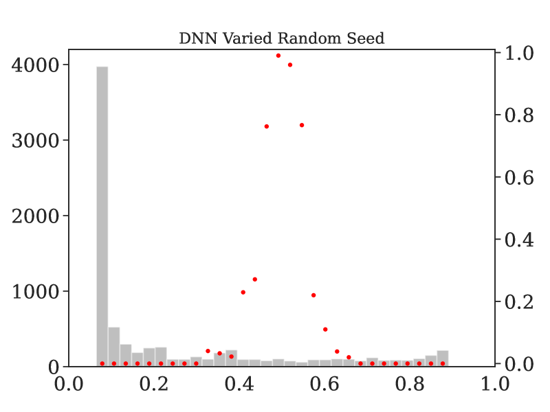
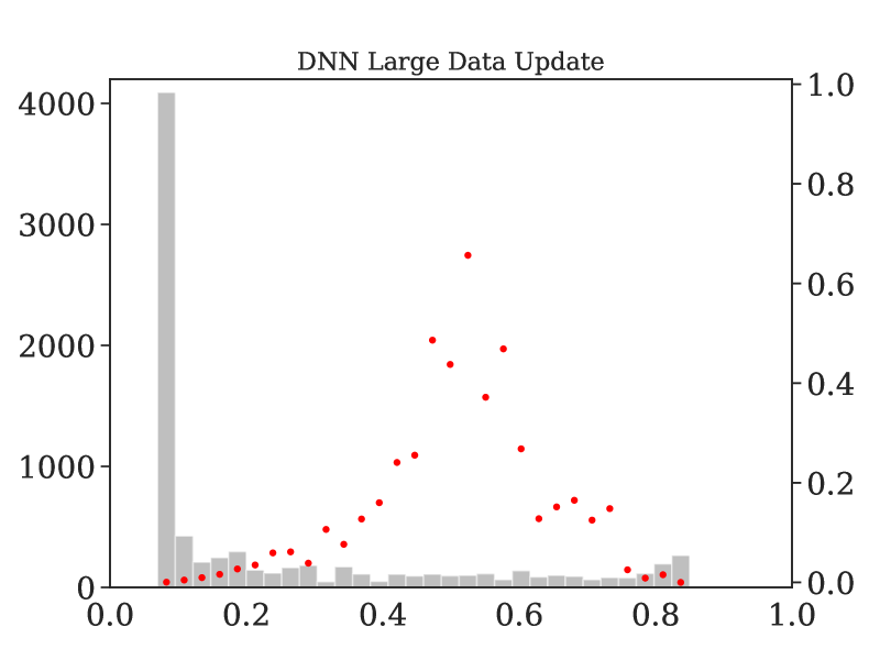
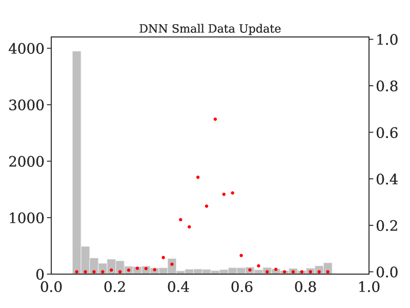
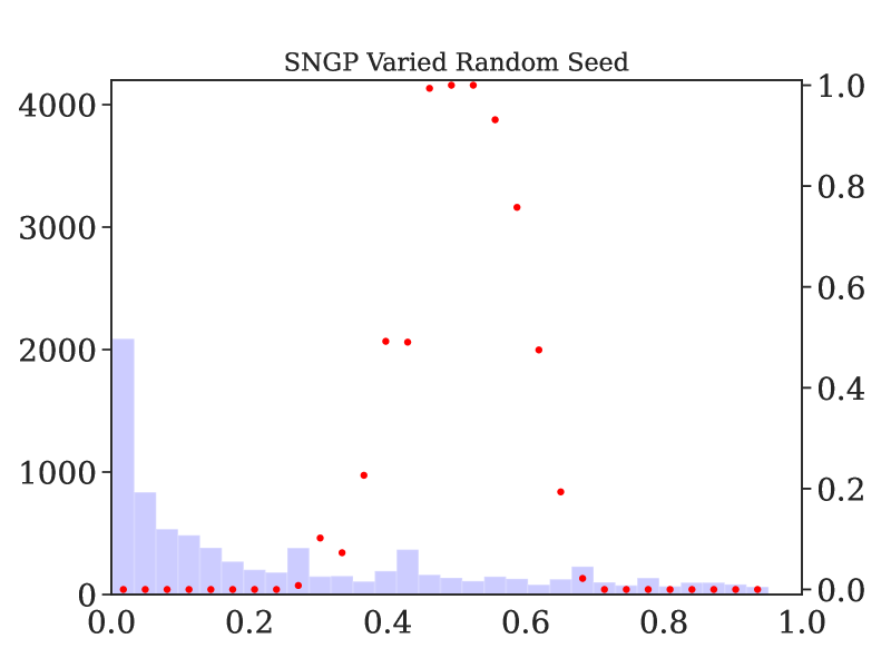
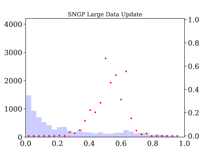
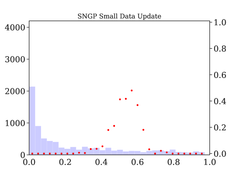
Figure 1: Predicted probability distributions for the Adult Dataset. We plot a histogram of predicted probability distribution in grey with the left $y$-axis and a scatter plot of the proportion of flip counts for each bin aligned with the right $y$-axis. By overlapping the plots, we gain a comprehensive view of the model’s confidence in its predictions (via the histogram) and the areas where the model predictions are most prone to change (scatter plot of flips). Notice that the scale is different between the histogram and the flip counts. The top row corresponds to the DNN experiments and the bottom row are the UA-DNN experiments. Each column represents an experiment. From the left, we show results for predictive multiplicity, large dataset update, and small dataset update.

5.1 Setup

Datasets. We consider datasets with varying sample size, number of features, and class imbalance; summary statistics for each dataset are in Table 3.  As we show below, models trained and tested on these datasets exhibit notable variation in predictive inconsistency.

Metrics. We measure predictive inconsistency by computing the measures detailed in § 2. In terms of predictive multiplicity, we compute the empirical $\epsilon$-Rashomon set and report $\epsilon$-ambiguity over a test sample according to either Eq (5) or Eq (12). In terms of predictive churn, we report over a test sample according to Eq. (1).

Churn Regimes. We compute predictive churn Eq. (1) for different types of successive training updates according to literature on predictive churn [22]. First, we imitate a large dataset update by comparing Model $B$ ($h_{B}$) trained on the full dataset to Model $A$ ($h_{A}$) trained on a random sample of half the dataset. Second, we imitate a small dataset update by comparing Model $B$ ($h_{B}$) trained on the full dataset to Model $A$ ($h_{A}$) trained on a random sample of $95\%$ the dataset – i.e. $5\%$ of examples have been dropped or added between the two models. These two updates are similar but represent two different regimes (see [33]). 

Model Classes. We consider two classes of deep neural networks (DNNs). We train a standard neural network made up of 1 or more fully connected layers and refer to this as DNN. We also train a DNN that incorporates an uncertainty awareness technique and refer to this as UA-DNN. For this demonstration, we implement the SNGP technique described in § 3.2 to train the uncertainty aware model, UA-DNN. To ensure the models are well calibrated, we tune the parameters within the SNGP technique and apply Platt scaling for the fully connected DNN.

Dataset	Model	Predictive Multiplicity (Empirical $\epsilon$-Ambiguity)	AUC	Predictive Churn (Large Data Update)	AUC	Predictive Churn (Small Data Update)	AUC
Adult	DNN	0.047 $\pm$ 0.003	0.89 $\pm$ 0.010	0.058 $\pm$ 0.004	0.89 $\pm$ 0.009	0.028 $\pm$ 0.004	0.89 $\pm$ 0.01
Credit	DNN	0.053 $\pm$ 0.004	0.89 $\pm$ 0.01	0.050 $\pm$ 0.004	0.89 $\pm$ 0.009	0.029 $\pm$ 0.004	0.89 $\pm$ 0.01
HMDA	DNN	0.021 $\pm$ 0.004	0.89 $\pm$ 0.011	0.042 $\pm$ 0.004	0.89 $\pm$ 0.009	0.007 $\pm$ 0.004	0.89 $\pm$ 0.01
Adult	UA-DNN	0.12 $\pm$ 0.010	0.87 $\pm$ 0.015	0.074 $\pm$ 0.011	0.84 $\pm$ 0.012	0.041 $\pm$ 0.008	0.87 $\pm$ 0.016
Credit	UA-DNN	0.10 $\pm$ 0.010	0.87 $\pm$ 0.015	0.067 $\pm$ 0.012	0.84 $\pm$ 0.012	0.05 $\pm$ 0.008	0.87 $\pm$ 0.016
HMDA	UA-DNN	0.14 $\pm$ 0.010	0.87 $\pm$ 0.015	0.12 $\pm$ 0.011	0.84 $\pm$ 0.013	0.06 $\pm$ 0.008	0.87 $\pm$ 0.016

Table 1: This table shows that predictions are more sensitive to model perturbations (multiplicity) and an uncertainty-aware (UA) model can exhibit higher ambiguity compared to a standard DNN. We compare predictive multiplicity and predictive churn across datasets and model specifications. Over a held out sample $\mathcal{S}_{\textit{test}}$, we compute empirical $\epsilon$-ambiguity, $\alpha_{\epsilon}({\hat{\mathcal{R}}^{m}_{\epsilon}{}})$, as well as churn, $C{}(h_{A},h_{B})$, induced by a large or small data update. We also show the range of AUC over runs for each.

5.2 Results

Predictive Multiplicity vs Predictive Churn.

We investigate whether the severity of predictive churn between Model $A$ and Model $B$ is captured by predictive multiplicity analysis on only Model $A$. Findings for the Standard DNN and UA-DNN are shown in Table 1. Notably, we see that model performance, as measured by accuracy, is largely uniform across the table: neither model specification (DNN vs UA-DNN) nor random seed/data perturbations (columns) seem to affect overall predictive performance. Thus, under standard criteria for evaluating ML models, differences in prediction across these models could be considered to be “arbitrary”, with the corresponding implications for fairness discussed above.

We highlight several notable patterns. First, although they are measured on similar scales, predictive multiplicity as measured via ambiguity tends to be larger than predictive churn. Thus, in the settings that we study, predictions appear to be broadly more sensitive to model perturbations than to data updates. But only by a small amount. In terms of gauging the severity of potential predictive arbitrariness, analyzing ambiguity may help to anticipate predictive churn.

Second, within model specifications (DNN or UA-DNN), predictive multiplicity and predictive churn measurements generally align. Specifically, when a model exhibits high predictive multiplicity on one dataset relative to others, it also exhibits high predictive churn (across both churn regimes) relative to other datasets. Thus, for a given model, it is possible that the same properties of the dataset drive predictive multiplicity and predictive churn.

However, interestingly, between the DNN and UA-DNN specifications, we see that different datasets exhibit high prediction instability. For example, while DNN exhibits high(er) predictive multiplicity on Credit, the UA-DNN exhibits higher predictive multiplicity on HMDA but relatively lower on Credit. This highlights that arbitrariness in predictions is driven by an interaction between the dataset and the model specification, not by the data itself; echoing predictive arbitrariness studies from algorithmic fairness [21]. Importantly, this also highlights that a particular model specification may not be a general solution for mitigating arbitrariness across all settings.

Comparison of Unstable Sets.

We examine whether examples that are unstable over the update between Model $A$ and Model $B$ are included in those flagged as unstable when only using the $\epsilon$-Rashomon set of Model $A$. We study the broad patterns highlighted above in more detail by comparing the $\epsilon$-Rashomon unstable set to the churn unstable set for a given test sample $\mathcal{S}_{\textit{test}}$. For a given dataset, we take a heldout test sample and compute $\mathcal{S}^{\mathcal{R}}_{\textit{unstable}}{}(\mathcal{S}_{\textit{test}})$ and $\mathcal{S}^{\mathcal{C}}_{\textit{unstable}}{}(\mathcal{S}_{\textit{test}})$ described in § 3. Given that $\#\{\mathcal{S}^{\mathcal{R}}_{\textit{unstable}}{}(\mathcal{S}_{\textit{test}})\}$ tends to be greater than $\#\{\mathcal{S}^{\mathcal{C}}_{\textit{unstable}}{}(\mathcal{S}_{\textit{test}})\}$, we calculate what proportion of test examples in $\#\{\mathcal{S}^{\mathcal{C}}_{\textit{unstable}}{}(\mathcal{S}_{\textit{test}})\}$ are contained in $\#\{\mathcal{S}^{\mathcal{R}}_{\textit{unstable}}{}(\mathcal{S}_{\textit{test}})\}$ and report this common arbitrariness.

For instance, if all the examples in $\mathcal{S}_{\textit{test}}$ that churn are contained in the $\epsilon$-Rashomon unstable set, then the common arbitrariness would be $100\%$. If none of the examples in $\mathcal{S}_{\textit{test}}$ that churn are contained in the $\epsilon$-Rashomon unstable set then the common arbitrariness would be $0\%$. Results are show in Table 2. As expected, for the small data updates, the common arbitrariness is much higher than compared to the large data update. Comparing model classes, the UA-DNN for small dataset updates seems to recover the largest overlap ranging between $81\%$ to $91\%$ across datasets.

Predicted Probabilities and Unstable Examples.

Finally, we examine how predicted probabilities relate to which points are identified as unstable. With the $\epsilon$-Rashomon unstable set and the churn unstable sets over a given test sample, we visualize the number of unstable examples alongside the full predicted probability distribution in Figure 1. First, we plot a histogram of the predicted probabilities for the test sample. Then, for each bin of the histogram, we compute the counts of the unstable (flipped) examples within that bin. Namely, the number of unstable (flipped) examples in a bin divided by the total number of predictions in that bin. This highlights where the model’s predictions are most unstable or uncertain as indicated by a higher proportion of unstable points.

We see that predicted probabilities are similarly concentrated in the middle of the unit interval comparing DNN to UA-DNN, which is somewhat surprising given the explicit consideration of uncertainty in UA-DNN. But one side effect of this consideration is that small perturbations may send UA-DNN predictions across the default decision boundary, which could explain the generally higher rates of arbitrariness in Table 1, especially under the predictive multiplicity perspective.

The findings suggests that UA-DNN models can provide useful indications of which examples are more at risk of being unstable under perturbations of the UA-DNN model, as a result of both predictive multiplicity or churn. Importantly, however, we find that UA-DNN predicted probabilities do not correlate well with unstable examples under the DNN model, so the utility of the uncertainty quantification done by UA-DNN is model-specific.

Model Uncertainty and Unstable Examples.

We explore how model uncertainty can also flag unstable examples from the $\epsilon$-Rashomon or churn perspective. We plot an uncertainty threshold against the proportion of unstable examples over within the unstable set in Figure 2. Here, we compute uncertainty using as $p(1-p)$ where $p$ is the predicted probability (a common approach in classification). For UA-DNN using the SNGP technique, this corresponds to an estimate of the posterior predictive (see § 3.2). We find that on average, predictive multiplicity and churn (small update regime) are well correlated with model uncertainty for UA-DNN. For DNN, across datasets, the relationship between uncertainty and arbitrariness varies.

Dataset	Model	Predictive Churn (Large Data Update)	Predictive Churn (Small Data Update)
Adult	DNN	0.58	0.73
Credit	DNN	0.47	0.85
HDMA	DNN	0.68	0.78
Adult	UA-DNN	0.64	0.91
Credit	UA-DNN	0.67	0.81
HDMA	UA-DNN	0.44	0.81

Table 2: This table shows the $\epsilon$-Rashomon unstable set tends to contain many of the examples within the churn unstable set. We report common flipped examples across different experiments i.e. the proportion of churned examples that are included in the $\epsilon$-Rashomon unstable set.

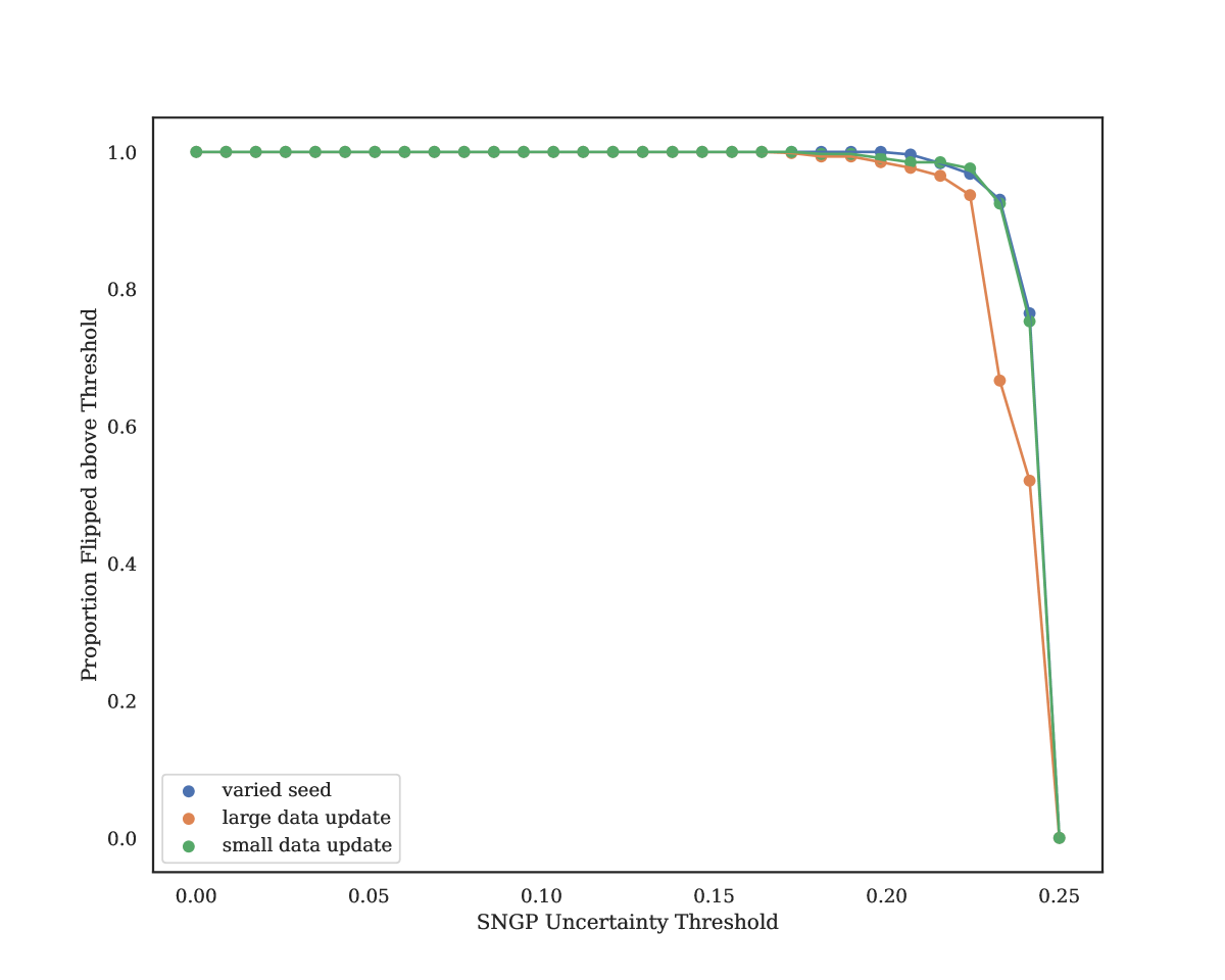
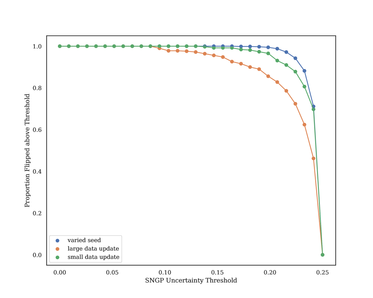
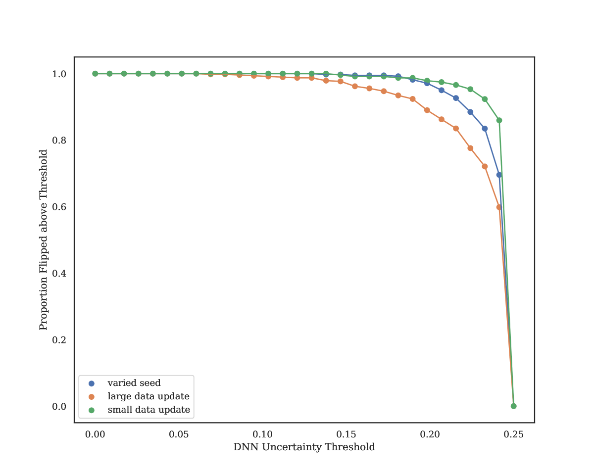
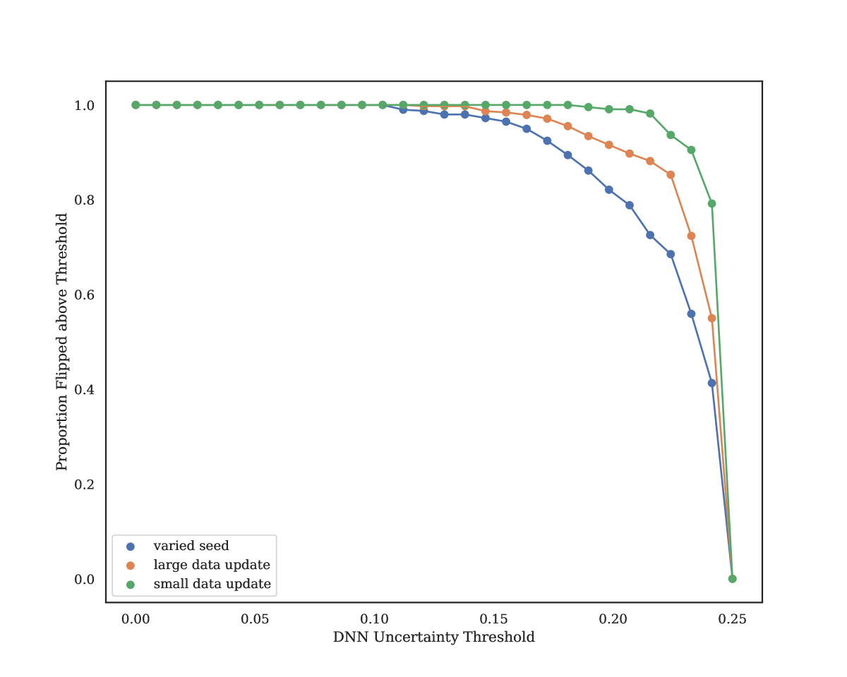
Figure 2: An uncertainty aware (UA) model produces uncertainty estimates that indicate unstable instances from both perspectives. These plots show the relationship between model uncertainty estimates and the arbitrariness of predictions for UCI Census (left) and Credit (right). We plot the uncertainty threshold ($x$-axis) versus the proportion of unstable examples that exceed the uncertainty threshold ($y$-axis). The proportion is the number of unstable (flipped) predictions with uncertainty $\geq$ a given threshold divided by the total number of unstable (flipped) predictions for this test sample. For each uncertainty threshold, we plot results for large dataset update (orange), small dataset update (green), and predictive multiplicity (blue). Here, the top is UA-DNN and the bottom is DNN.

6 Implications

Our findings reveal that analyzing predictive multiplicity is a useful way to anticipate predictive churn over time. We can consider the set of prospective models around the selected deployed model and draw conclusions about anticipated predictive churn. Given that research in predictive multiplicity has largely focused on how to measure its severity and methods to train the $\epsilon$-Rashomon set, the present study demonstrates how predictive multiplicity can help assess an important notion of predictive instability (churn).

To combine predictive multiplicity and churn, a practitioner could conduct one analysis after the other. For choosing a better starting point while anticipating model updates, we can begin with a predictive multiplicity analysis following by a predictive churn analysis. Say for instance, we have a model $A$ that we are considering for deployment. We can ask if there might exist a model within the $\epsilon$-Rashomon set for which the anticipated churn is likely less than that of model $A$. To do this, we can train the $\epsilon$-Rashomon set with model $A$ as a baseline then evaluate changes in the churn unstable set for each model within the Rashomon set. We can also train the $\epsilon$-Rashomon set without assuming a baseline and choose the model that might minimize expected churn from that.

Previous studies have examined various churn reduction methods [22; 38]. It will be interesting in future work to examine whether known churn reduction methods (e.g., distillation and constrained weight optimization) might improve predictive multiplicity. To do this, we would analyze predictive multiplicity over a standard training procedure then, make improvements to said training procedure that for churn reduction and analyze predictive multiplicity over this improved training procedure. Similar to our empirical demonstrations, you can then take a fixed test set and compare the $\epsilon$-Rashomon unstable set against the churn unstable set. Ultimately, this would provide insight into whether training procedures that are more robust to churn are also more robust to predictive multiplicity. And, in line with bridging between uncertainty quantification and fairness as arbitrariness, future work can also explore additional methods from reliable deep learning i.e  [77].

7 Conclusion

Reducing arbitrariness in machine learning is critical for machine learning credibility and reproducibility. This goal aligns with efforts to address arbitrariness as as a form of unfairness. In particular, fairness researchers underline the challenge in justifying the use of predictions to inform decision making when there exists equally good models that might change individual outcomes [10]. We advocate for connecting the fairness/safety perspective to research on reliable and robust learning. This study is an initial step in that direction.

Appendix A Omitted Proofs

Proof of Proposition 4.3.

This follows from the triangle inequality. For a set $S=\{x_{1},\ldots,x_{n}\}$, we denote the predictions as vectors:

$$Y_{1}=(h_{1}(x_{1}),...,h_{1}(x_{n}))\in\{0,1\}^{n}$$

$$Y_{2}=(h_{2}(x_{1}),...,h_{2}(x_{n}))\in\{0,1\}^{n}$$

Let $Y$ denote the ground-truth label,

$$Y=(y_{1},...,y_{n})\in\{0,1\}^{n}.$$

The empirical risk $\hat{R}{}$ of a classifier can be expressed in terms of the $L_{1}$ norm between the predictions and the ground truth:

$$\hat{R}{}(h_{1})=\frac{||Y_{1}-Y||_{1}}{n},\quad\hat{R}{}(h_{2})=\frac{||Y_{2}-Y||_{1}}{n}$$

Similarly, we write churn as the $L_{1}$ norm between the predictions of the two models.

$$C{}(h_{1},h_{2})=\frac{||Y_{1}-Y_{2}||_{1}}{n}$$

The triangle inequality results in:

$$||Y_{1}-Y_{2}||_{1}\leq||Y_{1}-Y||_{1}+||Y-Y_{2}||_{1}$$

Substitution and dividing by $n$ gives

$$C{}(h_{1},h_{2})\leq\hat{R}{}(h_{1})+\hat{R}{}(h_{2}).$$

∎

Proof of Corollary 4.4.

By definition, $\hat{R}(h{}^{\prime})\leq\hat{R}(h{}_{0})+\epsilon$. Following Proposition 4.3, we have:

$$\!C{}(h{}_{0},h{}^{\prime})\! \leq\hat{R}{}(h_{0})+\hat{R}{}(h{}^{\prime})\leq 2\hat{R}{}(h{}_{0})+\epsilon.$$ (10)

∎

Proof of Lemma 4.5.

We use linearity of expectation and the assumption that models in $\mathcal{T}_{\mathcal{D}_{A}}$ are sampled i.i.d. to show that the difference in expectation is $0$.

$$\mathbb{E}_{h{}_{A},h{}^{\prime}_{A}\stackrel{{\scriptstyle iid}}{{\sim}}\mathcal{T}_{\textit{rand}}{}(\mathcal{D}{}_{A})}\left[C{}(h{}_{A},h{}_{B})-C{}(h{}^{\prime}_{A},h{}_{B})\right]$$

$$=\mathbb{E}_{h{}_{A}\stackrel{{\scriptstyle iid}}{{\sim}}\mathcal{T}_{\textit{rand}}{}(\mathcal{D}{}_{A})}[C{}(h{}_{A},h{}_{B})]$$

$$\quad-\mathbb{E}_{h{}^{\prime}_{A}\stackrel{{\scriptstyle iid}}{{\sim}}\mathcal{T}_{\textit{rand}}{}(\mathcal{D}{}_{A})}[C{}(h{}^{\prime}_{A},h{}_{B}))]$$

$$=\mathbb{E}_{h{}_{A}\stackrel{{\scriptstyle iid}}{{\sim}}\mathcal{T}_{\textit{rand}}{}(\mathcal{D}{}_{A})}[\mathbb{E}_{(X,Y)\sim\mathcal{D}{}}[\ell_{0,1}(h{}_{A}(X),Y)-\ell_{0,1}(h{}_{B})(X),Y)]]$$

$$\quad-\mathbb{E}_{h{}^{\prime}_{A}\stackrel{{\scriptstyle iid}}{{\sim}}\mathcal{T}_{\textit{rand}}{}(\mathcal{D}{}_{A})}[\mathbb{E}_{(X,Y)\sim\mathcal{D}{}}[\ell_{0,1}(h{}^{\prime}_{A}(X),Y)-\ell_{0,1}(h{}_{B})(X),Y)]]$$

$$=\mathbb{E}_{h{}_{A},h{}^{\prime}_{A}\stackrel{{\scriptstyle iid}}{{\sim}}\mathcal{T}_{\textit{rand}}{}(\mathcal{D}{}_{A})}[\mathbb{E}_{(X,Y)\sim\mathcal{D}{}}[\ell_{0,1}(h{}_{A}(X),Y)-\ell_{0,1}(h{}^{\prime}_{A}(X),Y)]]$$

$$=\mathbb{E}_{h{}_{A}\stackrel{{\scriptstyle iid}}{{\sim}}\mathcal{T}_{\textit{rand}}{}(\mathcal{D}{}_{A})}[\mathbb{E}_{(X,Y)\sim\mathcal{D}{}}[\ell_{0,1}(h{}_{A}(X),Y)]]-\mathbb{E}_{h{}^{\prime}_{A}\stackrel{{\scriptstyle iid}}{{\sim}}\mathcal{T}_{\textit{rand}}{}(\mathcal{D}{}_{A})}[\mathbb{E}_{(X,Y)\sim\mathcal{D}}[\ell_{0,1}(h{}^{\prime}_{A}(X),Y)]]$$

$$=0.$$

∎

Proof of Theorem 4.2.

We first state the results from  Cormier et al. [2016].

Theorem A.1 (Bound on Expected Churn [Cormier et al., 2016]).

Assuming a training algorithm that is $\beta$-stable, given training datasets $\mathcal{D}_{A}$ and $\mathcal{D}_{B}$, sampled i.i.d. from $\mathcal{D}{}^{n}$ where two classifiers $h{}_{A}$ and $h{}_{B}$ are trained on $\mathcal{D}_{A}$ and $\mathcal{D}_{B}$ respectively, the expected smooth churn obeys:

$$\mathbbm{E}_{\mathcal{D}_{A},\mathcal{D}_{B}\sim\mathcal{D}^{n}}\left[C_{\gamma}(h{}_{A},h{}_{B})\right]\leq\frac{\beta\sqrt{\pi n}}{\gamma}.$$ (11)

From Theorem A.1, the smooth churn between the two baseline models is bounded by:

$$\mathbbm{E}_{\mathcal{D}_{A},\mathcal{D}_{B}\sim\mathcal{D}^{m}}[C{}_{\gamma}(h{}_{0}^{A},h{}_{0}^{B})]\leq\frac{\beta\sqrt{\pi n}}{\gamma}.$$

The churn between any two models within the $\epsilon$-Rashomon sets, $\mathcal{R}_{\epsilon}({h{}_{0}^{A}})$ and $\mathcal{R}_{\epsilon}({h{}_{0}^{B}})$, is bounded by this constant plus a new $2\epsilon$ term. To show this, we apply the triangle inequality and Lemma 4.5, working with any pair of models, $h{}^{\prime}_{A}\in\mathcal{R}_{\epsilon}({h_{0}^{A}})$ and $h{}^{\prime}_{B}\in\mathcal{R}_{\epsilon}({h{}_{0}^{B}})$:

$$\mathbbm{E}_{\mathcal{D}_{A},\mathcal{D}_{B}\sim\mathcal{D}^{m}}[C{}_{\gamma}(h{}^{\prime}_{A},h{}^{\prime}_{B})]$$

$$=\mathbbm{E}_{(X,Y)\sim\mathcal{D}}\left[\ell_{\gamma}(h{}^{\prime}_{A}(X),Y)-\ell_{\gamma}(h{}^{\prime}_{B},Y)\right]$$

$$=\mathbbm{E}_{(X,Y)\sim\mathcal{D}}[\ell_{\gamma}(h{}^{\prime}_{A}(X),Y)+\ell_{\gamma}(h{}^{A}_{0}(X),Y)$$

$$-\ell_{\gamma}(h{}^{A}_{0}(X),Y)+\ell_{\gamma}(h{}^{B}_{0}(X),Y)-\ell_{\gamma}(h{}^{B}_{0}(X),Y)$$

$$-\ell_{\gamma}(h{}^{\prime}_{B},Y)]$$

$$=\mathbbm{E}_{(X,Y)\sim\mathcal{D}}\left[\ell_{\gamma}(h{}^{\prime}_{A}(X),Y)-\ell_{\gamma}(h{}^{A}_{0}(X),Y)\right]$$

$$+\mathbbm{E}_{(X,Y)\sim\mathcal{D}}\left[\ell_{\gamma}(h{}^{A}_{0}(X),Y)-\ell_{\gamma}(h{}^{B}_{0}(X),Y)\right]$$

$$+\mathbbm{E}_{(X,Y)\sim\mathcal{D}}\left[\ell_{\gamma}(h{}^{B}_{0}(X),Y)-\ell_{\gamma}(h{}^{\prime}_{B},Y)\right]$$

$$\leq\epsilon+\frac{\beta\sqrt{\pi n}}{\gamma}+\epsilon=\frac{\beta\sqrt{\pi n}}{\gamma}+2\epsilon,$$

where the second and third equalities are algebra. For the inequality, the first and third expectations follow from the Definition of smooth churn and the middle expectation from Theorem A.1. For the final equality, we appeal to Definition 2.2, with $\ell_{\gamma}$ as the performance metric and $\epsilon$ being the parameter of the Rashomon set. ∎

Appendix B Additional Definitions

Predictive Multiplicity

As an example of a training procedure that approximates the empirical $\epsilon$-Rashomon set with respect to a baseline model, we review the following. As noted in the main paper, these two metrics for quantifying predictive multiplicity reflect the proportion of examples in a sample $S$ that are assigned conflicts (or “flips”) over the $\epsilon$-Rashomon set.

Definition B.1 ($\epsilon$-Ambiguity w.r.t. $h_{0}$).

The ambiguity of a prediction problem w.r.t. $h{}_{0}$ is the proportion of examples $i\in S$ assigned a conflicting prediction by a classifier in the $\epsilon$-Rashomon set:

$$\!\alpha_{\epsilon}({h{}_{0}})\!:=\!\frac{1}{|S|}\sum_{i\in S}\max_{h\in\mathcal{R}_{\epsilon}({h{}_{0}})}\mathbbm{1}[h(x_{i})\neq h_{0}(x_{i})].$$ (12)

Definition B.2 (Discrepancy w.r.t. $h_{0}$).

The discrepancy of a prediction problem w.r.t. $h{}_{0}$ is the maximum proportion of examples $i\in S$ assigned a conflicting prediction by a single competing classifier in the $\epsilon$-Rashomon set:

$$\!\delta_{\epsilon}({h{}_{0}})\!:=\!\max_{h\in\mathcal{R}_{\epsilon}({h{}_{0}})}\frac{1}{|S|}\sum_{i\in S}\mathbbm{1}[h(x_{i})\neq h_{0}(x_{i})].$$ (13)

Ambiguity characterizes the number of individuals whose predictions are sensitive to model choice with respect to the set of near-optimal models. In domains where predictions inform decisions (e.g., loan approval or recidivism risk), individuals with ambiguous decisions could contest the prediction assigned to them. In contrast, discrepancy measures the maximum number of predictions that can change by replacing the baseline model with another near-optimal model.

An approach to compute these metrics is to approximate the Rashomon set by directly perturbing the target loss in training Marx et al. [2019], Watson-Daniels et al. [2023b, a]. We denote this loss-targeting method as $\mathcal{T}_{\textit{perturb}}{}(h{}_{0},\mathcal{D}{})\subseteq\mathcal{H}$, and it returns a set of hypotheses in the $\epsilon$-Rashomon set. For shorthand notation, we leave implicit in the sequel the baseline and dataset in notation $\mathcal{T}_{\textit{perturb}}{}$.

Definition B.3 (Empirical $\epsilon$-Rashomon set w.r.t. $h{}_{0}$).

Given a performance metric $M$, an error tolerance $\epsilon>0$, and a baseline model $h{}_{0}$, the empirical $\epsilon$-Rashomon set w.r.t. $h{}_{0}$ is the set of competing classifiers $h\in\mathcal{H}$ induced by $\mathcal{T}_{\textit{perturb}}{}$:

$$\hat{\mathcal{R}}_{\epsilon}{}(\mathcal{T}_{\textit{perturb}}{})\!:=\!\{h{}\,:\,h{}\in\mathcal{T}_{\textit{perturb}}{},M(h{};\mathcal{D}{})\leq M(h{}_{0};\mathcal{D}{})+\epsilon\}.$$ (14)

An example of $\mathcal{T}_{\textit{perturb}}{}$

Here is an example of $\mathcal{T}_{\textit{perturb}}{}$. Watson-Daniels et al. [2023b] introduced a method for computing ambiguity and discrepancy that involves training the Rashomon set as follows. A set of candidate models are trained via constrained optimization such that $P(\hat{y}_{i}=+1)$ is constrained to the threshold $p$ as in Eq. (15). From that set of candidate models, those with near-optimal performance are selected.

1:  Input: data $\{(x_{i},y_{i})\}_{i=1}^{n}$

2:  Input: baseline model $\{h_{0}{(x_{i})}\}_{i=1}^{n}$

3:  Input: threshold probabilities $P$

4:  Input: error tolerance $\epsilon$

5:  for $i\in\{(x_{i},y_{i})\}_{i=1}^{n}$ do

6:     Initialize $x_{p},y_{p}=X(i),Y(i)$

7:     for $p\in P$ do

8:       $h\leftarrow$ model from Eq. (15)

9:       $pr(x_{p})\leftarrow$ $h{(x_{p})}$

10:     end for

11:  end for

12:  candidate models $\in\{h,pr(x_{p})\}_{i\in[n],p\in P}$

13:  $\epsilon$-Rashomon set $\leftarrow$ candidate models that perform within $\epsilon$ of $h_{0}$

14:  Output: $\epsilon$-Rashomon set

Algorithm 1 Constructing the $\epsilon$-Rashomon set

Definition B.4 (Candidate Model).

Given a baseline model $h_{0}$, a finite set of user-specified threshold probabilities $P\subseteq[0,1]$, then for each $p\in P$ a candidate model for example $x_{i}$ is an optimal solution to the following constrained empirical risk minimization problem:

$$\begin{split}\min_{w\in\mathbb{R}^{d+1}}&\ L(w)\\ \textnormal{s.t.}\quad&h(x_{i})\leq p,\;\;\textrm{if}~{}p<h_{0}(x_{i})\\ &h(x_{i})\geq p.\;\;\;\textrm{if}~{}p>h_{0}(x_{i})\end{split}$$ (15)

This technique can be applied to any convex loss function $L(\cdot)$ including a convex regularization term. Watson-Daniels et al. [2023b] illustrate the methodology on a probabilistic classification task with logistic regression where $h(x_{i})=\frac{1}{1+\exp(-\langle w,x_{i}\rangle)}$.

Appendix C Experiment Details

Dataset Name	Outcome Variable	$n$	$d$	Class Imbalance
Adult [Kohavi, 1996]	person income over $50,000	16,256	28	0.31
HMDA [Cooper et al., 2023]	loan granted	244,107	18	3.3
Credit [Yeh and Lien, 2009]	customer default on loan	30,000	23	3.50

Table 3: Datasets used in the experiments. For each dataset, we report $n$, $d$ and the class imbalance ratio of a model on test data.

Models

All models use a shallow neural network with 1 or more fully connected layers. There is 1 hidden layer with 279 units, learning rate of 0.0000579, dropout rate of 0.0923 and batch normalization is enabled. All training is conducted in TensorFlow with a batch size of 128. When training sets of models, we use multiple arrays of random seeds $\{0.0,1.0,109,10,1234\}$, $\{3666,2299,2724,1262,4220\}$, $\{3971,9444,1375,7351,2083\}$, $\{1429,2281,2189,9376,2261\}$ and $\{1881,2273,9509,6707,4412\}$. For varying random initialisations, we repeat experiments across these arrays. For churn experiments, we use the first random seed in the array as the default seed and repeat experiments across these values. We run on a single CPU with 50GB RAM.

The SNGP training process follows the standard DNN learning pipeline, with the updated Gaussian process and spectral normalization outputting predictive logits and posterior covariance. For a test example, the model posterior mean and covariance are used to compute the predictive distribution. Specifically, we approximate the posterior predictive probability, $E(p(x))$, using the mean-field method $E(p(x))\sim\text{softmax}\left(\text{logit}(x)/\sqrt{1+\lambda*\sigma^{2}(x)}\right)$, where $\sigma^{2}(x)$ is the SNGP variance and $\lambda$ is a hyperparameter, tuned for optimal model calibration (in deep learning, this is known as temperature scaling [Guo et al., 2017]).

Appendix D Additional Results

For two additional datasets, we plot a histogram of predicted probability distribution in grey with the left $y$-axis and a scatter plot of the proportion of flip counts for each bin aligned with the right $y$-axis. By overlapping the plots, we gain a comprehensive view of the model’s confidence in its predictions (via the histogram) and the areas where the model predictions are most prone to change (scatter plot of flips). Notice that the scale is different between the histogram and the flip counts. The top row corresponds to the DNN experiments and the bottom row are the UA-DNN experiments. Each column represents an experiment. From the left, we show results for predictive multiplicity, large dataset update, and small dataset update.

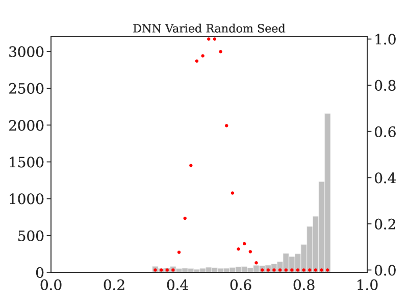
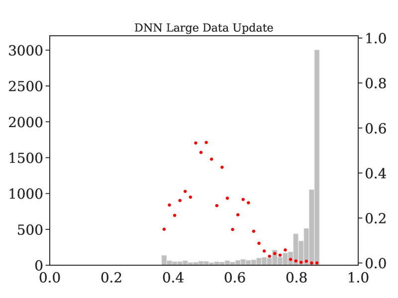
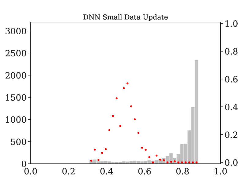
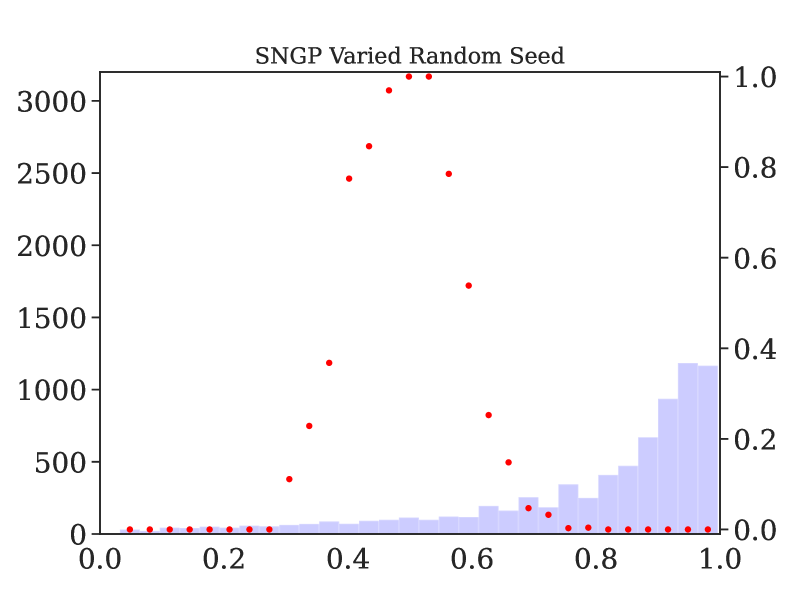
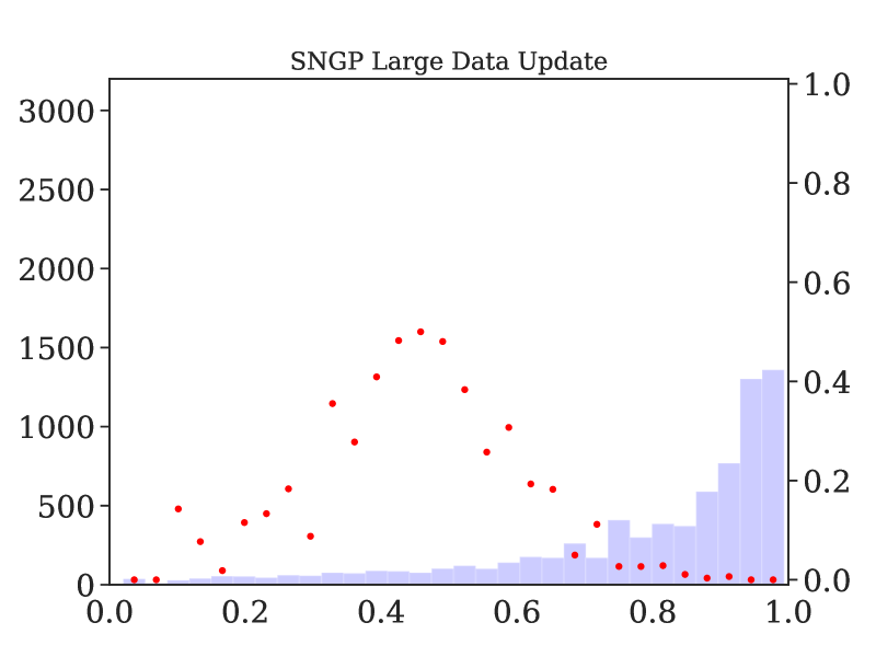
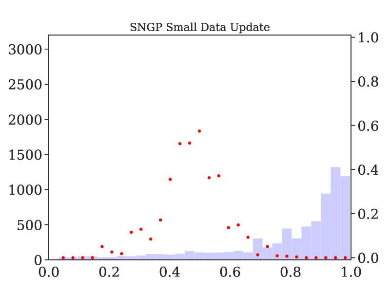
Figure 3: Predicted probability distributions for Credit Dataset.

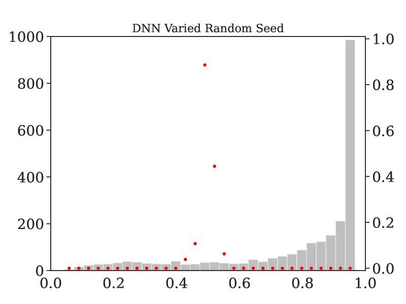
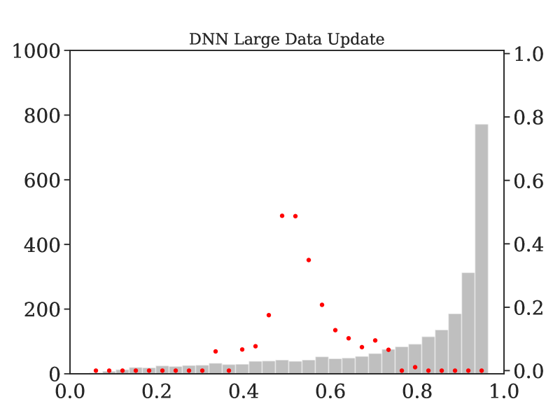
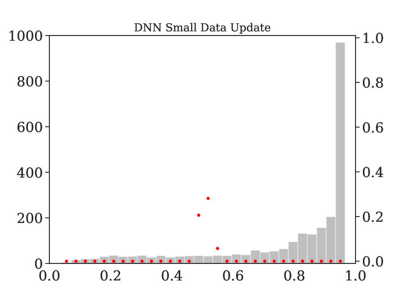
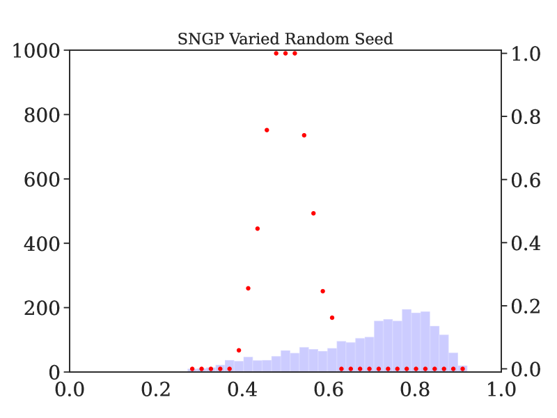
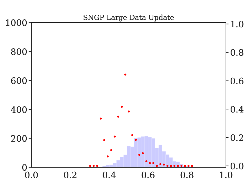
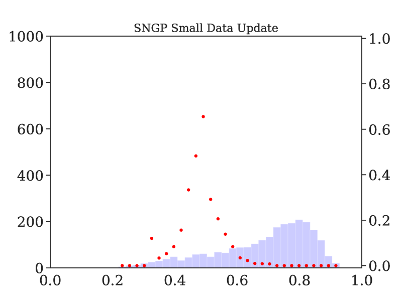
Figure 4: Predicted probability distributions for HDMA Dataset.

References

- Ali et al. [2021] Junaid Ali, Preethi Lahoti, and Krishna P. Gummadi. Accounting for Model Uncertainty in Algorithmic Discrimination. Association for Computing Machinery, 2021. ISBN 9781450384735. doi: 10.1145/3461702.3462630.
- Anil et al. [2018] Rohan Anil, Gabriel Pereyra, Alexandre Tachard Passos, Robert Ormandi, George Dahl, and Geoffrey Hinton. Large scale distributed neural network training through online distillation. In ICLR, 2018. URL https://openreview.net/pdf?id=rkr1UDeC-.
- Attigeri et al. [2017] Girija V. Attigeri, M. M.Manohara Pai, and Radhika M. Pai. Credit risk assessment using machine learning algorithms. Advanced Science Letters, 23(4):3649–3653, 2017. ISSN 19367317. doi: 10.1166/asl.2017.9018.
- Bahri and Jiang [2021] Dara Bahri and Heinrich Jiang. Locally adaptive label smoothing for predictive churn, 2021.
- Bekhet and Eletter [2014] Hussain Ali Bekhet and Shorouq Fathi Kamel Eletter. Credit risk assessment model for Jordanian commercial banks: Neural scoring approach. Review of Development Finance, 4(1):20–28, 2014. ISSN 18799337. doi: 10.1016/j.rdf.2014.03.002. URL http://dx.doi.org/10.1016/j.rdf.2014.03.002.
- Belkin et al. [2019] Mikhail Belkin, Daniel Hsu, Siyuan Ma, and Soumik Mandal. Reconciling modern machine-learning practice and the classical bias–variance trade-off. Proceedings of the National Academy of Sciences, 116(32):15849–15854, 2019. doi: 10.1073/pnas.1903070116. URL https://www.pnas.org/doi/abs/10.1073/pnas.1903070116.
- Bendale and Boult [2016] A. Bendale and T. E. Boult. Towards open set deep networks. In 2016 IEEE Conference on Computer Vision and Pattern Recognition (CVPR), pages 1563–1572, Los Alamitos, CA, USA, jun 2016. IEEE Computer Society. doi: 10.1109/CVPR.2016.173. URL https://doi.ieeecomputersociety.org/10.1109/CVPR.2016.173.
- Biesialska et al. [2020] Magdalena Biesialska, Katarzyna Biesialska, and Marta R. Costa-jussà. Continual lifelong learning in natural language processing: A survey. In Proceedings of the 28th International Conference on Computational Linguistics, pages 6523–6541, Barcelona, Spain (Online), December 2020. International Committee on Computational Linguistics. doi: 10.18653/v1/2020.coling-main.574. URL https://aclanthology.org/2020.coling-main.574.
- Black and Fredrikson [2021] Emily Black and Matt Fredrikson. Leave-one-out Unfairness. ACM Conference on Fairness, Accountability, and Transparency, 2021.
- Black et al. [2022] Emily Black, Manish Raghavan, and Solon Barocas. Model multiplicity: Opportunities, concerns, and solutions. In 2022 ACM Conference on Fairness, Accountability, and Transparency, pages 850–863, 2022.
- Blundell et al. [2015] Charles Blundell, Julien Cornebise, Koray Kavukcuoglu, and Daan Wierstra. Weight uncertainty in neural networks. In Proceedings of the 32nd International Conference on International Conference on Machine Learning - Volume 37, ICML’15, page 1613–1622. JMLR.org, 2015.
- Bousquet and Elisseeff [2000] Olivier Bousquet and André Elisseeff. Algorithmic stability and generalization performance. In T. Leen, T. Dietterich, and V. Tresp, editors, Advances in Neural Information Processing Systems, volume 13. MIT Press, 2000. URL https://proceedings.neurips.cc/paper_files/paper/2000/file/49ad23d1ec9fa4bd8d77d02681df5cfa-Paper.pdf.
- Breiman [2001] Leo Breiman. Statistical modeling: The two cultures. Statistical Science, 16(3):199–215, 2001. ISSN 08834237. doi: 10.1214/ss/1009213726.
- Buckheit and Donoho [1995] Jonathan B. Buckheit and David L. Donoho. Wavelab and reproducible research. In Wavelets and Statistics, 1995. URL https://api.semanticscholar.org/CorpusID:16424339.
- Cai et al. [2022] Deng Cai, Elman Mansimov, Yi-An Lai, Yixuan Su, Lei Shu, and Yi Zhang. Measuring and reducing model update regression in structured prediction for NLP. In Alice H. Oh, Alekh Agarwal, Danielle Belgrave, and Kyunghyun Cho, editors, Advances in Neural Information Processing Systems, 2022. URL https://openreview.net/forum?id=4cdxptfCCg.
- Calandra et al. [2016] Roberto Calandra, Jan Peters, Carl Edward Rasmussen, and Marc Peter Deisenroth. Manifold gaussian processes for regression, 2016.
- Chatfield [1995] Chris Chatfield. Model Uncertainty, Data Mining and Statistical Inference. Journal of the Royal Statistical Society. Series A (Statistics in Society), 158(3):419, 1995. ISSN 09641998. doi: 10.2307/2983440.
- Chen et al. [2018] Zhiyuan Chen, Bing Liu, Ronald Brachman, Peter Stone, and Francesca Rossi. Lifelong Machine Learning. Morgan & Claypool Publishers, 2nd edition, 2018. ISBN 1681733021.
- Choi et al. [2019] Dami Choi, Christopher J. Shallue, Zachary Nado, Jaehoon Lee, Chris J. Maddison, and George E. Dahl. On empirical comparisons of optimizers for deep learning. CoRR, abs/1910.05446, 2019. URL http://arxiv.org/abs/1910.05446.
- Cooper et al. [2021] A. Feder Cooper, Yucheng Lu, Jessica Forde, and Christopher M De Sa. Hyperparameter Optimization Is Deceiving Us, and How to Stop It. In M. Ranzato, A. Beygelzimer, Y. Dauphin, P.S. Liang, and J. Wortman Vaughan, editors, Advances in Neural Information Processing Systems, volume 34, pages 3081–3095. Curran Associates, Inc., 2021.
- Cooper et al. [2023] A. Feder Cooper, Katherine Lee, Madiha Zahrah Choksi, Solon Barocas, Christopher De Sa, James Grimmelmann, Jon Kleinberg, Siddhartha Sen, and Baobao Zhang. Is my prediction arbitrary? the confounding effects of variance in fair classification benchmarks, 2023.
- Cormier et al. [2016] Q. Cormier, M. Milani Fard, K. Canini, and M. R. Gupta. Launch and iterate: Reducing prediction churn. In D. Lee, M. Sugiyama, U. Luxburg, I. Guyon, and R. Garnett, editors, Advances in Neural Information Processing Systems, volume 29. Curran Associates, Inc., 2016. URL https://proceedings.neurips.cc/paper_files/paper/2016/file/dc5c768b5dc76a084531934b34601977-Paper.pdf.
- Coston et al. [2021] Amanda Coston, Ashesh Rambachan, and Alexandra Chouldechova. Characterizing Fairness Over the Set of Good Models Under Selective Labels. ICML, 2021. URL http://arxiv.org/abs/2101.00352.
- Cotter et al. [2019] Andrew Cotter, Heinrich Jiang, Serena Wang, Taman Narayan, Seungil You, Karthik Sridharan, and Maya R. Gupta. Optimization with non-differentiable constraints with applications to fairness, recall, churn, and other goals. Journal of Machine Learning Research, 2019.
- Dong and Rudin [2019] Jiayun Dong and Cynthia Rudin. Variable Importance Clouds: A Way to Explore Variable Importance for the Set of Good Models. Nature Machine Intelligence, 2019. URL http://arxiv.org/abs/1901.03209.
- Donnelly et al. [2023] Jon Donnelly, Srikar Katta, Cynthia Rudin, and Edward P Browne. The rashomon importance distribution: Getting RID of unstable, single model-based variable importance. In Thirty-seventh Conference on Neural Information Processing Systems, 2023. URL https://openreview.net/forum?id=TczT2jiPT5.
- D’Amour et al. [2020] Alexander D’Amour, Katherine Heller, Dan Moldovan, Ben Adlam, Babak Alipanahi, Alex Beutel, Christina Chen, Jonathan Deaton, Jacob Eisenstein, Matthew D. Hoffman, Farhad Hormozdiari, Neil Houlsby, Shaobo Hou, Ghassen Jerfel, Alan Karthikesalingam, Mario Lucic, Yian Ma, Cory McLean, Diana Mincu, Akinori Mitani, Andrea Montanari, Zachary Nado, Vivek Natarajan, Christopher Nielson, Thomas F. Osborne, Rajiv Raman, Kim Ramasamy, Rory Sayres, Jessica Schrouff, Martin Seneviratne, Shannon Sequeira, Harini Suresh, Victor Veitch, Max Vladymyrov, Xuezhi Wang, Kellie Webster, Steve Yadlowsky, Taedong Yun, Xiaohua Zhai, and D. Sculley. Underspecification presents challenges for credibility in modern machine learning. arXiv, 2020. ISSN 23318422.
- Farquhar et al. [2020] Sebastian Farquhar, Michael A. Osborne, and Yarin Gal. Radial bayesian neural networks: Beyond discrete support in large-scale bayesian deep learning. In Silvia Chiappa and Roberto Calandra, editors, Proceedings of the Twenty Third International Conference on Artificial Intelligence and Statistics, volume 108 of Proceedings of Machine Learning Research, pages 1352–1362. PMLR, 26–28 Aug 2020. URL https://proceedings.mlr.press/v108/farquhar20a.html.
- Fisher et al. [2019] Aaron Fisher, Cynthia Rudin, and Francesca Dominici. All models are wrong, but many are useful: Learning a variable’s importance by studying an entire class of prediction models simultaneously. Journal of Machine Learning Research, 20(Vi), 2019. ISSN 15337928.
- Gal and Ghahramani [2016] Yarin Gal and Zoubin Ghahramani. Dropout as a bayesian approximation: Representing model uncertainty in deep learning, 2016.
- Gentleman and Lang [2007] Robert Gentleman and Duncan Temple Lang. Statistical analyses and reproducible research. Journal of Computational and Graphical Statistics, 16(1):1–23, 2007. doi: 10.1198/106186007X178663. URL https://doi.org/10.1198/106186007X178663.
- Gepperth and Hammer [2016] Alexander Gepperth and Barbara Hammer. Incremental learning algorithms and applications. In European Symposium on Artificial Neural Networks (ESANN), Bruges, Belgium, 2016. URL https://hal.science/hal-01418129.
- Giordano et al. [2019] Ryan Giordano, William Stephenson, Runjing Liu, Michael Jordan, and Tamara Broderick. A swiss army infinitesimal jackknife. In Kamalika Chaudhuri and Masashi Sugiyama, editors, Proceedings of the Twenty-Second International Conference on Artificial Intelligence and Statistics, volume 89 of Proceedings of Machine Learning Research, pages 1139–1147. PMLR, 16–18 Apr 2019. URL https://proceedings.mlr.press/v89/giordano19a.html.
- Goh et al. [2016] Gabriel Goh, Andrew Cotter, Maya Gupta, and Michael P Friedlander. Satisfying real-world goals with dataset constraints. In D. Lee, M. Sugiyama, U. Luxburg, I. Guyon, and R. Garnett, editors, Advances in Neural Information Processing Systems, volume 29. Curran Associates, Inc., 2016. URL https://proceedings.neurips.cc/paper_files/paper/2016/file/dc4c44f624d600aa568390f1f1104aa0-Paper.pdf.
- Guo et al. [2017] Chuan Guo, Geoff Pleiss, Yu Sun, and Kilian Q. Weinberger. On calibration of modern neural networks. In Doina Precup and Yee Whye Teh, editors, Proceedings of the 34th International Conference on Machine Learning, volume 70 of Proceedings of Machine Learning Research, pages 1321–1330. PMLR, 06–11 Aug 2017. URL https://proceedings.mlr.press/v70/guo17a.html.
- Hooker et al. [2020] Sara Hooker, Nyalleng Moorosi, Gregory Clark, Samy Bengio, and Emily Denton. Characterising bias in compressed models, 2020.
- Hsu and Calmon [2022] Hsiang Hsu and Flavio du Pin Calmon. Rashomon capacity: A metric for predictive multiplicity in classification, 2022. URL https://arxiv.org/abs/2206.01295.
- Jiang et al. [2022] Heinrich Jiang, Harikrishna Narasimhan, Dara Bahri, Andrew Cotter, and Afshin Rostamizadeh. Churn reduction via distillation. In International Conference on Learning Representations, 2022. URL https://openreview.net/forum?id=HbtFCX2PLq0.
- Khand et al. [2017] Aleem Khand, Freddy Frost, Ruth Grainger, Michael Fisher, Pei Chew, Liam Mullen, Billal Patel, Mohammed Obeidat, Khaled Albouaini, James Dodd, Sarah A. Goldstein, L. Kristin Newby, Derek D. Cyr, Megan Neely, Thomas F. Lüscher, Eileen B. Brown, Harvey D. White, E. Magnus Ohman, Matthew T. Roe, Christian W. Hamm, A J Six, B E Backus, and J C Kelder. Heart Score Value. Netherlands Heart Journal, 10(6):1–10, 2017. ISSN 1568-5888.
- Kohavi [1996] Ron Kohavi. Census Income. UCI Machine Learning Repository, 1996. DOI: https://doi.org/10.24432/C5GP7S.
- Kovačević [2007] Jelena Kovačević. How to encourage and publish reproducible research. In 2007 IEEE International Conference on Acoustics, Speech and Signal Processing, ICASSP ’07, ICASSP, IEEE International Conference on Acoustics, Speech and Signal Processing - Proceedings, pages IV1273–IV1276, 2007. ISBN 1424407281. doi: 10.1109/ICASSP.2007.367309. Copyright: Copyright 2011 Elsevier B.V., All rights reserved.; 2007 IEEE International Conference on Acoustics, Speech and Signal Processing, ICASSP ’07 ; Conference date: 15-04-2007 Through 20-04-2007.
- Kristiadi et al. [2020] Agustinus Kristiadi, Matthias Hein, and Philipp Hennig. Being bayesian, even just a bit, fixes overconfidence in relu networks. In Proceedings of the 37th International Conference on Machine Learning, ICML’20. JMLR.org, 2020.
- Kulynych et al. [2023] Bogdan Kulynych, Hsiang Hsu, Carmela Troncoso, and Flavio P. Calmon. Arbitrary decisions are a hidden cost of differentially private training. In 2023 ACM Conference on Fairness, Accountability, and Transparency. ACM, jun 2023. doi: 10.1145/3593013.3594103. URL https://doi.org/10.1145%2F3593013.3594103.
- Lakshminarayanan et al. [2017] Balaji Lakshminarayanan, Alexander Pritzel, and Charles Blundell. Simple and scalable predictive uncertainty estimation using deep ensembles. In Proceedings of the 31st International Conference on Neural Information Processing Systems, NIPS’17, page 6405–6416, Red Hook, NY, USA, 2017. Curran Associates Inc. ISBN 9781510860964.
- Lan et al. [2018] Xu Lan, Xiatian Zhu, and Shaogang Gong. Knowledge distillation by on-the-fly native ensemble. In Proceedings of the 32nd International Conference on Neural Information Processing Systems, NIPS’18, page 7528–7538, Red Hook, NY, USA, 2018. Curran Associates Inc.
- Liu et al. [2020] Jeremiah Zhe Liu, Zi Lin, Shreyas Padhy, Dustin Tran, Tania Bedrax-Weiss, and Balaji Lakshminarayanan. Simple and principled uncertainty estimation with deterministic deep learning via distance awareness. In Proceedings of the 34th International Conference on Neural Information Processing Systems, NIPS’20, Red Hook, NY, USA, 2020. Curran Associates Inc. ISBN 9781713829546.
- Long et al. [2023] Carol Xuan Long, Hsiang Hsu, Wael Alghamdi, and Flavio P. Calmon. Arbitrariness lies beyond the fairness-accuracy frontier, 2023.
- Mackay [1992] David John Cameron Mackay. Bayesian Methods for Adaptive Models. PhD thesis, California Institute of Technology, USA, 1992. UMI Order No. GAX92-32200.
- Macêdo and Ludermir [2022] David Macêdo and Teresa Ludermir. Enhanced isotropy maximization loss: Seamless and high-performance out-of-distribution detection simply replacing the softmax loss, 2022.
- Malinin and Gales [2018] Andrey Malinin and Mark Gales. Predictive uncertainty estimation via prior networks. In Proceedings of the 32nd International Conference on Neural Information Processing Systems, NIPS’18, page 7047–7058, Red Hook, NY, USA, 2018. Curran Associates Inc.
- Marx et al. [2019] Charles Marx, Flavio P. Calmon, and Berk Ustun. Predictive multiplicity in classification, 2019.
- Masana et al. [2023] M. Masana, X. Liu, B. Twardowski, M. Menta, A. D. Bagdanov, and J. van de Weijer. Class-incremental learning: Survey and performance evaluation on image classification. IEEE Transactions on Pattern Analysis and Machine Intelligence, 45(05):5513–5533, may 2023. ISSN 1939-3539. doi: 10.1109/TPAMI.2022.3213473.
- McNutt [2014] Marcia McNutt. Reproducibility. Science, 343(6168):229–229, 2014. doi: 10.1126/science.1250475. URL https://www.science.org/doi/abs/10.1126/science.1250475.
- Mei and Montanari [2022] Song Mei and Andrea Montanari. The generalization error of random features regression: Precise asymptotics and the double descent curve. Communications on Pure and Applied Mathematics, 75(4):667–766, 2022. doi: https://doi.org/10.1002/cpa.22008. URL https://onlinelibrary.wiley.com/doi/abs/10.1002/cpa.22008.
- Mesirov [2010] Jill P. Mesirov. Accessible reproducible research. Science, 327(5964):415–416, 2010. doi: 10.1126/science.1179653. URL https://www.science.org/doi/abs/10.1126/science.1179653.
- Meyer et al. [2023] Anna P. Meyer, Aws Albarghouthi, and Loris D’Antoni. The dataset multiplicity problem: How unreliable data impacts predictions. In Proceedings of the 2023 ACM Conference on Fairness, Accountability, and Transparency, FAccT ’23, page 193–204, New York, NY, USA, 2023. Association for Computing Machinery. ISBN 9798400701924. doi: 10.1145/3593013.3593988. URL https://doi.org/10.1145/3593013.3593988.
- Moreno et al. [2005] Rui P. Moreno, Philipp G.H. Metnitz, Eduardo Almeida, Barbara Jordan, Peter Bauer, Ricardo Abizanda Campos, Gaetano Iapichino, David Edbrooke, Maurizia Capuzzo, and Jean Roger Le Gall. SAPS 3 - From evaluation of the patient to evaluation of the intensive care unit. Part 2: Development of a prognostic model for hospital mortality at ICU admission. Intensive Care Medicine, 31(10):1345–1355, 2005. ISSN 03424642. doi: 10.1007/s00134-005-2763-5.
- Nakkiran et al. [2019] Preetum Nakkiran, Gal Kaplun, Yamini Bansal, Tristan Yang, Boaz Barak, and Ilya Sutskever. Deep double descent: Where bigger models and more data hurt, 2019.
- Neal [1996] Radford M. Neal. Bayesian Learning for Neural Networks. Springer-Verlag, Berlin, Heidelberg, 1996. ISBN 0387947248.
- Ovadia et al. [2019] Yaniv Ovadia, Emily Fertig, Jie Ren, Zachary Nado, D. Sculley, Sebastian Nowozin, Joshua V. Dillon, Balaji Lakshminarayanan, and Jasper Snoek. Can You Trust Your Model’s Uncertainty? Evaluating Predictive Uncertainty under Dataset Shift. Curran Associates Inc., Red Hook, NY, USA, 2019.
- Parisi et al. [2019] German I. Parisi, Ronald Kemker, Jose L. Part, Christopher Kanan, and Stefan Wermter. Continual lifelong learning with neural networks: A review. Neural Networks, 113:54–71, 2019. ISSN 0893-6080. doi: https://doi.org/10.1016/j.neunet.2019.01.012. URL https://www.sciencedirect.com/science/article/pii/S0893608019300231.
- Pawelczyk et al. [2020] Martin Pawelczyk, Klaus Broelemann, and Gjergji Kasneci. On counterfactual explanations under predictive multiplicity. Proceedings of the 36th Conference on Uncertainty in Artificial Intelligence, UAI 2020, 124:839–848, 2020.
- Peng [2011] Roger D. Peng. Reproducible research in computational science. Science, 334(6060):1226–1227, 2011. doi: 10.1126/science.1213847. URL https://www.science.org/doi/abs/10.1126/science.1213847.
- Polikar et al. [2001] R. Polikar, L. Upda, S. S. Upda, and V. Honavar. Learn++: An incremental learning algorithm for supervised neural networks. Trans. Sys. Man Cyber Part C, 31(4):497–508, nov 2001. ISSN 1094-6977. doi: 10.1109/5326.983933. URL https://doi.org/10.1109/5326.983933.
- Qian et al. [2021] Shangshu Qian, Viet Hung Pham, Thibaud Lutellier, Zeou Hu, Jungwon Kim, Lin Tan, Yaoliang Yu, Jiahao Chen, and Sameena Shah. Are my deep learning systems fair? an empirical study of fixed-seed training. In M. Ranzato, A. Beygelzimer, Y. Dauphin, P.S. Liang, and J. Wortman Vaughan, editors, Advances in Neural Information Processing Systems, volume 34, pages 30211–30227. Curran Associates, Inc., 2021. URL https://proceedings.neurips.cc/paper_files/paper/2021/file/fdda6e957f1e5ee2f3b311fe4f145ae1-Paper.pdf.
- Riquelme et al. [2018] Carlos Riquelme, George Tucker, and Jasper Snoek. Deep bayesian bandits showdown: An empirical comparison of bayesian deep networks for thompson sampling. In International Conference on Learning Representations, 2018. URL https://openreview.net/forum?id=SyYe6k-CW.
- Rule et al. [2018] Adam Rule, Amanda Birmingham, Cristal Zuniga, Ilkay Altintas, Shih-Cheng Huang, Rob Knight, Niema Moshiri, Mai H. Nguyen, Sara Brin Rosenthal, Fernando Pérez, and Peter W. Rose. Ten simple rules for reproducible research in jupyter notebooks, 2018.
- Semenova et al. [2019] Lesia Semenova, Cynthia Rudin, and Ronald Parr. A study in Rashomon curves and volumes: A new perspective on generalization and model simplicity in machine learning. Arxiv, pages 1–64, 2019. URL http://arxiv.org/abs/1908.01755.
- Sensoy et al. [2018] Murat Sensoy, Lance Kaplan, and Melih Kandemir. Evidential deep learning to quantify classification uncertainty. In Proceedings of the 32nd International Conference on Neural Information Processing Systems, NIPS’18, page 3183–3193, Red Hook, NY, USA, 2018. Curran Associates Inc.
- Shen et al. [2020] Y. Shen, Y. Xiong, W. Xia, and S. Soatto. Towards backward-compatible representation learning. In 2020 IEEE/CVF Conference on Computer Vision and Pattern Recognition (CVPR), pages 6367–6376, Los Alamitos, CA, USA, jun 2020. IEEE Computer Society. doi: 10.1109/CVPR42600.2020.00640. URL https://doi.ieeecomputersociety.org/10.1109/CVPR42600.2020.00640.
- Shu et al. [2017] Lei Shu, Hu Xu, and Bing Liu. DOC: Deep open classification of text documents. In Proceedings of the 2017 Conference on Empirical Methods in Natural Language Processing, pages 2911–2916, Copenhagen, Denmark, September 2017. Association for Computational Linguistics. doi: 10.18653/v1/D17-1314. URL https://aclanthology.org/D17-1314.
- Snoek et al. [2015] Jasper Snoek, Oren Rippel, Kevin Swersky, Ryan Kiros, Nadathur Satish, Narayanan Sundaram, Md. Mostofa Ali Patwary, Prabhat Prabhat, and Ryan P. Adams. Scalable bayesian optimization using deep neural networks. In Proceedings of the 32nd International Conference on International Conference on Machine Learning - Volume 37, ICML’15, page 2171–2180. JMLR.org, 2015.
- Song and Chai [2018] Guocong Song and Wei Chai. Collaborative learning for deep neural networks. In Proceedings of the 32nd International Conference on Neural Information Processing Systems, NIPS’18, page 1837–1846, Red Hook, NY, USA, 2018. Curran Associates Inc.
- Sonnenburg et al. [2007] Sören Sonnenburg, Mikio L. Braun, Cheng Soon Ong, Samy Bengio, Leon Bottou, Geoffrey Holmes, Yann LeCun, Klaus-Robert Müller, Fernando Pereira, Carl Edward Rasmussen, Gunnar Rätsch, Bernhard Schölkopf, Alexander Smola, Pascal Vincent, Jason Weston, and Robert Williamson. The need for open source software in machine learning. J. Mach. Learn. Res., 8:2443–2466, dec 2007. ISSN 1532-4435.
- Tagasovska and Lopez-Paz [2019] Natasa Tagasovska and David Lopez-Paz. Single-Model Uncertainties for Deep Learning. Curran Associates Inc., Red Hook, NY, USA, 2019.
- Than et al. [2014] Martin Than, Dylan Flaws, Sharon Sanders, Jenny Doust, Paul Glasziou, Jeffery Kline, Sally Aldous, Richard Troughton, Christopher Reid, William A. Parsonage, Christopher Frampton, Jaimi H. Greenslade, Joanne M. Deely, Erik Hess, Amr Bin Sadiq, Rose Singleton, Rosie Shopland, Laura Vercoe, Morgana Woolhouse-Williams, Michael Ardagh, Patrick Bossuyt, Laura Bannister, and Louise Cullen. Development and validation of the emergency department assessment of chest pain score and 2h accelerated diagnostic protocol. EMA - Emergency Medicine Australasia, 26(1):34–44, 2014. ISSN 17426731. doi: 10.1111/1742-6723.12164.
- Tran et al. [2022] Dustin Tran, Jeremiah Liu, Michael W. Dusenberry, Du Phan, Mark Patrick Collier, Jie Jessie Ren, Kehang Han, Zi Wang, Zelda Mariet, Clara Huiyi Hu, Neil Band, Tim G. J. Rudner, Karan Singhal, Zachary Nado, Joost van Amersfoort, Andreas Christian Kirsch, Rodolphe Jenatton, Nithum Thain, Honglin Yuan, Kelly Buchanan, Kevin Patrick Murphy, D. Sculley, Yarin Gal, Zoubin Ghahramani, Jasper Roland Snoek, and Balaji Lakshminarayanan. Plex: Towards reliability using pretrained large model extensions. In ICML Workshop: Principles of Distribution Shift (PODS), 2022.
- Träuble et al. [2021] Frederik Träuble, Julius Von Kügelgen, Matthäus Kleindessner, Francesco Locatello, Bernhard Schölkopf, and Peter Vincent Gehler. Backward-compatible prediction updates: A probabilistic approach. In A. Beygelzimer, Y. Dauphin, P. Liang, and J. Wortman Vaughan, editors, Advances in Neural Information Processing Systems, 2021. URL https://openreview.net/forum?id=YjZoWjTKYvH.
- van Amersfoort et al. [2020] Joost van Amersfoort, Lewis Smith, Yee Whye Teh, and Yarin Gal. Uncertainty estimation using a single deep deterministic neural network, 2020.
- Vanschoren et al. [2014] Joaquin Vanschoren, Mikio L. Braun, and Cheng Soon Ong. Open science in machine learning, 2014.
- Veitch et al. [2021] Victor Veitch, Alexander D’Amour, Steve Yadlowsky, and Jacob Eisenstein. Counterfactual invariance to spurious correlations: Why and how to pass stress tests. arXiv preprint arXiv:2106.00545, 2021.
- Watson-Daniels et al. [2023a] Jamelle Watson-Daniels, Solon Barocas, Jake M. Hofman, and Alexandra Chouldechova. Multi-target multiplicity: Flexibility and fairness in target specification under resource constraints. In Proceedings of the 2023 ACM Conference on Fairness, Accountability, and Transparency, FAccT ’23, page 297–311, New York, NY, USA, 2023a. Association for Computing Machinery. ISBN 9798400701924. doi: 10.1145/3593013.3593998. URL https://doi.org/10.1145/3593013.3593998.
- Watson-Daniels et al. [2023b] Jamelle Watson-Daniels, David C. Parkes, and Berk Ustun. Predictive Multiplicity in Probabilistic Classification. AAAI, pages 1–24, 2023b. URL http://arxiv.org/abs/2206.01131.
- Wei et al. [2022] Dennis Wei, Rahul Nair, Amit Dhurandhar, Kush R. Varshney, Elizabeth M. Daly, and Moninder Singh. On the safety of interpretable machine learning: A maximum deviation approach, 2022.
- Xie et al. [2021] Yuqing Xie, Yi an Lai, Yuanjun Xiong, Yi Zhang, and Stefano Soatto. Regression bugs are in your model! measuring, reducing and analyzing regressions in nlp model updates, 2021.
- Yan et al. [2021] S. Yan, Y. Xiong, K. Kundu, S. Yang, S. Deng, M. Wang, W. Xia, and S. Soatto. Positive-congruent training: Towards regression-free model updates. In 2021 IEEE/CVF Conference on Computer Vision and Pattern Recognition (CVPR), pages 14294–14303, Los Alamitos, CA, USA, jun 2021. IEEE Computer Society. doi: 10.1109/CVPR46437.2021.01407. URL https://doi.ieeecomputersociety.org/10.1109/CVPR46437.2021.01407.
- Yeh and Lien [2009] I. Cheng Yeh and Che hui Lien. The comparisons of data mining techniques for the predictive accuracy of probability of default of credit card clients. Expert Systems with Applications, 36(2 PART 1):2473–2480, 2009. ISSN 09574174. doi: 10.1016/j.eswa.2007.12.020. URL http://dx.doi.org/10.1016/j.eswa.2007.12.020.
- Zhang et al. [2017] Ying Zhang, Tao Xiang, Timothy M. Hospedales, and Huchuan Lu. Deep mutual learning, 2017.
- Zhong et al. [2023] Chudi Zhong, Zhi Chen, Jiachang Liu, Margo Seltzer, and Cynthia Rudin. Exploring and interacting with the set of good sparse generalized additive models. In Thirty-seventh Conference on Neural Information Processing Systems, 2023. URL https://openreview.net/forum?id=CzAAbKOHQW.