Beyond Sparsity: Local Projections Inference with High-Dimensional Covariates

Abstract

Impulse response analysis studies how the economy responds to shocks, such as changes in interest rates, and helps policymakers manage these effects. While Vector Autoregression Models (VARs) with structural assumptions have traditionally dominated the estimation of impulse responses, local projections, the projection of future responses on current shock, have recently gained attention for their robustness and interpretability. Including many lags as controls is proposed as a means of robustness, and including a richer set of controls helps in its interpretation as a causal parameter. In both cases, an extensive number of controls leads to the consideration of high-dimensional techniques. While methods like LASSO exist, they mostly rely on sparsity assumptions - most of the parameters are exactly zero, which has limitations in dense data generation processes. This paper proposes a novel approach that incorporates high-dimensional covariates in local projections without relying on sparsity constraints. Adopting the Orthogonal Greedy Algorithm with a high-dimensional AIC (OGA+HDAIC) model selection method, this approach offers advantages including robustness in both sparse and dense scenarios, improved interpretability by prioritizing cross-sectional explanatory power, and more reliable causal inference in local projections.

1 Introduction

Impulse responses analyze how a shock, such as a change in interest rates, affects various aspects of the economy over time. Knowing how different parts of the economy respond to shocks, such as policy changes or natural shocks, helps policymakers make informed decisions and helps businesses prepare for potential impacts. Traditionally, Vector Autoregression Models (VARs) with structural assumptions on how economic variables affect each other have been a central tool for estimating impulse responses. In recent years, local projections, introduced by Jordà (2005), have received considerable attention in the literature due to their robustness and interpretability. Notably, Montiel Olea and Plagborg-Møller (2021) have promoted local projection inference by demonstrating its robustness and simplicity under lag augmentation, using more lags as controls than the true autoregressive model suggested. Another intriguing aspect of local projection is its interpretation as a causal parameter, as proposed by Angrist et al. (2018a). According to their conceptual framework, the key identifying assumption is the conditional independence assumption. One of the primary motivations for high-dimensional studies is that introducing large sets of covariates makes the conditional independence assumption more plausible(D’Amour et al. (2021), Rosenbaum and Rosenbaum (2002)). However, extensive lag augmentation and controlling for an increasing number of covariates can introduce computational challenges and potential overfitting concerns, especially in large systems.

Beyond local projections, recent research in high-dimensional time series analysis has addressed this challenge: see, for example, Masini et al. (2023) for a review of machine learning techniques in time series forecasting. Chernozhukov et al. (2021) explored the use of double/ debiased LASSO with temporal and cross-sectional dependence, building on the Gaussian approximation results of Zhang and Wu (2017). Babii et al. (2022) tackled both the high-dimensional and mixed-frequency settings by adopting the sparse group-LASSO method, which allows inference on a low-dimensional group of parameters. Finally, Adamek et al. (2023a) proposed a debiased/ desparsified LASSO method with near epoch dependence (NED) assumption, relaxing the mixing conditions. In the following paper, Adamek et al. (2023b) extend their work in the context of local projections. Compared to their previous paper, they obtain better finite sample performance by penalizing except for the impulse response parameter. Most of the work relies on LASSO, which comes with sparsity assumptions on the underlying parameters: only a handful of parameters are nonzero. While this provides a convenient way to perform model selection based on the underlying sparsity, it may not always be the case in real economic models.

The sparsity assumptions have been criticized in the literature, in particular by Giannone et al. (2021) and Kolesár et al. (2023). Employing a Bayesian inference method, Giannone et al. (2021) assess the validity of sparse or dense data-generating processes (DGPs). The authors find that including a more extensive set of covariates improves predictive power in several empirical applications, including macroeconomic examples relevant to impulse response analysis. Kolesár et al. (2023) specifically challenge the sparsity assumptions in linear regression models and highlight their fragility to the choice of regressors, such as choosing a different baseline category for categorical variables. Through empirical and theoretical analysis, they argue that the sparsity of the underlying model depends on the particular specification of the control matrix and suggest the possibility that there is no normalization of the control matrix that allows a sparse approximation. Both studies emphasize the need for proper verification of the model’s inherent sparsity. They propose testing procedures that often reject the sparsity assumptions, suggesting the need for alternative approaches that can effectively accommodate denser DGPs.

This paper addresses this shortcoming of LASSO-based methods, allowing for more efficient and reliable inference in a broader range of scenarios in the context of local projections. I employ a model selection method of Orthogonal Greedy Algorithm (OGA) with High dimensional AIC (HDAIC) by Ing (2020). The critical difference in the assumption is that there is no restriction on the number of parameters: we allow the parameters to be nonzero, but they should decay towards zero as the dimensionality grows. Admittedly, there is extensive literature using other methods that do not require sparsity assumptions, with a prominent example being Principal Component (PC) type methods (Stock and Watson (2002)). Borrowing arguments from Feng et al. (2020), albeit in a different framework, model selection methods have the advantage of selecting the important variables based on their importance in the “cross-section” of variables, as opposed to other PC-type methods that select factors based on their ability to explain the time-series variation of responses. Another strength of the proposed method is its interpretability. OGA first orders the covariates in descending order of their explanatory power, and then HDAIC selects the number of parameters to include in the model. Invoking the causal interpretation of the impulse response parameter as in Angrist et al. (2018a), the proposed method chooses cross-sectionally significant covariates to contribute to the validity of the conditional independence assumption.

Do these theoretical concerns on sparsity have practical implications for the performance and robustness in the context of impulse response analysis? In Adamek et al. (2023b), their assumption on the parameter is called weak sparsity, where they have a parameter $r\in[0,1)$ that allows the parameters to be not exactly sparse for $r\neq 0$. However, their simulation shows that their proposed estimator performs relatively poorly compared to the standard local projection estimator when the DGP is dense. This paper complements this point by highlighting that our assumptions do not require such sparsity assumptions, leading to superior finite sample performance in dense DGP settings. In an illustrative simulation study, I compare our proposed method with their method to evaluate finite sample performance in a high-dimensional VAR$(4)$ model with different settings of coefficient matrices. The evidence suggests that our method performs well regardless of whether the parameters are sparse or dense.

This paper extends the OGA+HDAIC method by Ing (2020) in the context of local projections, incorporating explicit assumptions on the dependence structure. In terms of the dependence structure, this paper aligns closely with Adamek et al. (2023a) and Adamek et al. (2023b) in using the NED assumption, as opposed to the dependence assumptions in Zhang and Wu (2017) and Chernozhukov et al. (2021). I have benefited enormously from the comprehensive foundation of dependence concepts and properties in the exquisite textbook Davidson (1994). A key advantage of using the NED assumption is that it inherits the mixingale properties that I employ in deriving the error bounds. Furthermore, I leverage the triplex inequality from Jiang (2009) in conjunction with the results in Ing (2020) to derive the inference of the proposed method.

The remainder of the paper is organized as follows. Section 2 presents the notations and details of the proposed method. Section 3 illustrates the finite sample performance of the proposed method on a high-dimensional VAR$(4)$ model with different settings of the coefficient matrices. Section 4 describes the definitions and assumptions and introduces the main theory. Section 5 includes concluding remarks.

2 Overview of the Method

Consider the following $h-$step ahead local projection regression model

$$y_{t+h}=\beta_{h}x_{t}+\delta_{h,0}^{\prime}\bm{r}_{t}+\sum_{\ell=1}^{L}\delta_{h,\ell}^{\prime}\bm{z}_{t-\ell}+u_{t,h},$$

where $y_{t+h}$ is the $h$-step ahead response variable, $x_{t}$ the innovation, $\bm{r}_{t}$ are contemporaneous controls, and $\bm{z}_{t}$ are lagged controls. The index $t=1,\dots,\bar{T}$ is an index for the observations, $h=1,\dots,H_{\max}$ is an index for horizons, and $\ell=1,\dots,L$ is the number of lags included in the model. Note that $x_{t}$ does not have to be a predetermined shock, although it can be thought of as predetermined if one wants to relate it to the structural assumptions of VAR models. This is a general representation of local projections in the literature, as introduced in Plagborg-Møller and Wolf (2021). Following the spirit of Jordà (2005), I fix $h$ and focus on each horizon of interest.

We are interested in the response of $y_{t+h}$ with respect to a shock in $x_{t}$, and our parameter of interest, the $h-$step ahead impulse response $\beta_{h}$, is defined as

$$\beta_{h}=E\left[y_{t+h}|x_{t}=1,\bm{r}_{t},\{\bm{z}_{t-\ell}\}_{\ell=1}^{L}\right]-E\left[y_{t+h}|x_{t}=0,\bm{r}_{t},\{\bm{z}_{t-\ell}\}_{\ell=1}^{L}\right].$$

For notation simplicity, stack the covariates except for $x_{t}$ into $\bm{w}_{t}=(\bm{r}_{t},\bm{z}_{t-1},\dots,\bm{z}_{t-L})$ and write

$$y_{t+h}=\beta_{h}x_{t}+\beta_{-h}^{\prime}\bm{w}_{t}+u_{t,h},$$ (2.1)

where $\beta_{-h}=(\delta_{h,0}^{\prime},\delta_{h,1}^{\prime},\dots,\delta_{h,L}^{\prime})^{\prime}$. Accounting for lag augmentations - adding more lags than identified by structural models - suggested by Montiel Olea and Plagborg-Møller (2021), the dimension of $\bm{w}_{t}$ grows as $L$ increases. Turning to the causal identification scheme of Angrist et al. (2018b), it is intuitive to add a large set of covariates as controls to account for unobserved counfounding variables, which also contributes to increasing the dimension of $\bm{w}_{t}$.

A straightforward approach to (2.1) with high dimensionality would be to apply a regularization method such as the LASSO. However, it is now well known that these methods come with an associated cost known as regularization bias. One way to address this challenge is a debiasing strategy using node-wise regression, regressing each covariate on the remaining covariates, as illustrated by Van de Geer et al. (2014) and Zhang and Zhang (2014). Using the estimates from the node-wise regressions, they construct a remedy for the bias term and control for it. An alternative approach is a double selection method that establishes an orthogonality condition in a similar spirit to Belloni et al. (2013). This method is analogous to the debiasing process of the LASSO, as noted in Semenova et al. (2023) and Chernozhukov et al. (2021). In the context of (2.1), the main idea of both approaches is to incorporate another set of regressions of the covariates to control for the regularization bias, either by debiasing or by using the covariates selected in both regression models.

In this paper, I consider the double selection method with a model selection method OGA+HDAIC by Ing (2020), where it consists of two steps. OGA first orders the covariates $\bm{w}_{t}$ by their explanatory power, and then we select the number of covariates that minimizes the high-dimensional AIC criteria. The selections come from the following regression models,

$$y_{t+h}= \lambda_{h}^{\prime}\bm{w}_{t}+e_{t,h},$$ (2.2)

$$x_{t}= \gamma_{h}^{\prime}\bm{w}_{t}+v_{t,{h}}.$$ (2.3)

Although not necessary in (2.3), I used the subscript $h$ for consistency across both equations. The concept involves applying OGA+HDAIC on both equations (2.2) and (2.3). To remove the regularization bias, I use the union of two selected covariates as $\bm{w}_{t}$ to finally run the local projection regression in (2.1). For a clear presentation of the OGA+HDAIC procedure, I fix some notations below.

Notations.

Let $t$ be an index for observations and $j$ for covariates, so that $\bm{w}_{t}=(w_{t,j})_{j=1}^{p}$ and $\bm{w}_{j}=(w_{t,j})_{t=1}^{T}$, where $p:=dim(\bm{w}_{t})$ and $T:=\bar{T}-h-L$ is the effective sample size. Let $[p]=1,\dots,p$ be the set of all covariate indices. Let $J$ be a set of covariate indices and let the subset of the covariates be $\bm{w}_{t}(J):=(w_{t,j})_{j\in J}$. Stack all $t=1,\dots,T$ observations of $\bm{w}_{t}(J)$ and denote $W(J):=(\bm{w}_{t}(J))_{t=1}^{T}$. Similarly define $\bm{y}_{h}=(y_{t+h})_{t=1}^{T}$. Denote the projection matrix using $W(J)$ as $P_{J}:=W(J)(W(J)^{\prime}W(J))^{-1}W(J)^{\prime}$.

First, consider the OGA part of $y_{t+h}$ on $\bm{w}_{t}$. The ordering of the covariates requires the following definition, which indicates the explanatory power of the covariate $\bm{w}_{i}$.

$$\mu_{i}(\emptyset)= {\bm{w}_{i}^{\prime}\bm{y}_{h}\over\sqrt{T}\left\lVert\bm{w}_{i}\right\rVert}={{1\over T}\bm{w}_{i}^{\prime}\bm{y}_{h}\over\sqrt{{1\over T}\bm{w}_{i}^{\prime}\bm{w}_{i}}},$$ (2.4)

As it looks, it works as a scaled version of a single regressor regression of $\bm{y}_{h}$ on each regressor $\bm{w}_{i}$. Since it is scaled by the square root of the $L_{2}$ norm of each regressor, the scale of $\bm{w}_{i}$ does not affect the magnitude of $\mu_{i}(J)$. To choose the one with the most explanatory power, we start with the setting $J=\emptyset$ and choose the one with the largest value of $\left|\mu_{i}(\emptyset)\right|$. Let this covariate index as

$$\widehat{j}_{1}:=\arg\min_{i\in[p]}\left|\mu_{i}(\emptyset)\right|,$$

and define the first chosen set as $\widehat{J}_{1}:=\{\widehat{j}_{1}\}$. To select the second order covariate, we use the residuals from the first step, using $\mu_{i}(\widehat{J}_{1})$ to measure explanatory power. We choose the second order covariate from the remaining covariates, $\widehat{j}_{2}:=\arg\min_{i\in[p]\setminus\widehat{J}_{1}}\left|\mu_{i}(\widehat{J}_{1})\right|$, then update the chosen set of covariates, $\widehat{J}_{2}=\widehat{J}_{1}\cup\{\widehat{j}_{2}\}$. Generalizing to the $m-$th order covariate, suppose we have the previously chosen set of covariates, $\widehat{J}_{m-1}$. Compute the following coefficient for all $i\in[p]\setminus\widehat{J}_{m-1}$, where

$$\mu_{i}(\widehat{J}_{m-1})= {\bm{w}_{i}^{\prime}(I-P_{\widehat{J}_{m-1}})\bm{y}_{h}\over\sqrt{T}\left\lVert\bm{w}_{i}\right\rVert},$$ (2.5)

and select the one with the largest absolute value of $\mu_{i}(\widehat{J}_{m-1})$,

$$\widehat{j}_{m}= \arg\min_{i\in[p]\setminus\widehat{J}_{m-1}}\left|\mu_{i}(\widehat{J}_{m-1})\right|,$$ (2.6)

and update the chosen set of covariates, $\widehat{J}_{m}=\widehat{J}_{m-1}\cup\{\widehat{j}_{m}\}$. Repeating this procedure orders the covariates in descending order of their explanatory power, conditioning on the previously chosen set of covariates. Now that the covariates are ordered, the remaining task is to select the threshold for the number of covariates. The information criterion we use is HDAIC, deinfed as

$$\text{HDAIC}(J)=\left(1+{C^{*}|J|\log p\over T}\right){\widehat{\sigma}}_{J}^{2},$$ (2.7)

where $\widehat{\sigma}_{J}^{2}=\bm{y}_{h}^{\prime}(I-P_{J})\bm{y}_{h}/T$. The number of covariates to be included in the model is the one which minimizes the information criteria,

$$\widehat{m}=\arg\min_{1\leq m\leq M_{T}^{*}}\text{HDAIC}(\widehat{J}_{m}).$$ (2.8)

Denote the chosen set of covariates as $\widehat{J}^{[1]}:=\widehat{J}_{\widehat{m}}$. Next, repeat the OGA+HDAIC for (2.3) and obtain the set of covariates $\widehat{J}^{[2]}$. Finally, denote the union set as $\widetilde{J}=\widehat{J}^{[1]}\cup\widehat{J}^{[2]}$ and run the local projection regression (2.1) with the selected covariates:

$$y_{t+h}=\beta_{h}x_{t}+\beta_{-h}^{\prime}\bm{w}_{t}(\widetilde{J})+u_{t,h}.$$

The least squares estimator for $\beta_{h}$ in this final model is our proposed estimator. For the variance estimator, define $\psi_{t}=v_{t,h}e_{t,h}$ and $\tau^{2}=E[\sum_{t=1}^{T}v_{t,h}^{2}/T]$. The variance estimator is then defined as

$$\widehat{\sigma}^{2}_{h}= {1\over\hat{\tau}^{2}}\widehat{\Omega},$$ (2.9)

$$\widehat{\Omega}= \sum_{\ell=-(K-1)}^{K-1}\left(1-{\ell\over K}\right){1\over T-\ell}\sum_{t=\ell+1}^{T}\widehat{\psi}_{t}\widehat{\psi}_{t-\ell},$$ (2.10)

where $\widehat{\Omega}$ is the Newey-West estimator with a bandwidth parameter $K$, which is assumed to be increasing with respect to increasing sample size. We borrow arguments from Andrews (1991) for the choice of $K$. $\widehat{\psi}_{t}$ is the sample analogue of $\psi_{t}$, where $\widehat{v}_{t,h}$ and $\widehat{e}_{t,h}$ are the residuals from (2.2) and (2.3).

The proposed algorithm is detailed in Algorithm 1 after a remark on tuning parameters.

Remark.

Unlike the OGA procedure, the HDAIC procedure has two unknown parameters, $M_{T}^{*}$ and $C^{*}$. A detailed description of both definitions can be found in Appendix C. $M_{T}^{*}$ is a parameter concerning the maximum number of covariates to include in the model and increases with $(T/\log p)$, as defined in (C.1). $C^{*}$, specified in (C.2), adjusts the penalty for dimensionality and is assumed to be greater than certain constants. While $C^{*}$ could be viewed as a tuning parameter, it’s more appropriately considered a hyperparameter, analogous to the hyperparameter of $2$ in traditional AIC. Aside from the plug-in option, there is a data-driven way to choose the value of $C^{*}$ by setting candidates, e.g. $\bar{C}=\{1.6,1.8,2,2.2,2.4\}$, and choosing the one that yields the smallest prediction errors in each regression in (2.2) and (2.3).

Algorithm 1.

[Double-OGA+HDAIC]

1. Compute $\mu_{i}(\emptyset)$ in (2.4) for all $i\in[p]$ and select the covariate with the largest $|\mu_{i}(\emptyset)|$. Denote the index of covariate as $\widehat{j}_{1}$ and define $\widehat{J}_{1}=\widehat{j}_{1}$.

2. Given $\widehat{J}_{1}$, compute $\mu_{i}(\widehat{J}_{1})$ for all $i\in[p]\setminus\widehat{J}_{1}$ and select the covariate with the largest $|\mu_{i}(\widehat{J}_{1})|$. Denote the index of covariate as $\widehat{j}_{2}$ and define $\widehat{J}_{2}=\widehat{J}_{1}\cup\widehat{j}_{2}$.

3. For $m>2$, compute $\mu_{i}(\widehat{J}_{m-1})$ for all $i\in[p]\setminus\widehat{J}_{m-1}$ and select the covariate with the largest $|\mu_{i}(\widehat{J}_{m-1})|$. Denote the index of covariate as $\widehat{j}_{m}$ and define $\widehat{J}_{m}=\widehat{J}_{m-1}\cup\widehat{j}_{m}$.

4. Compute HDAIC in (2.7) and select $m$ that minimizes HDAIC$(\widehat{J}_{m})$. Denote it as $\widehat{m}^{y}$ and define $\widehat{J}_{y}:=\widehat{J}_{\widehat{m}^{y}}$.

5. Run steps 1–4 by replacing $y_{t+h}$ with $x_{t}$. Obtain $\widehat{J}_{x}$ and the residuals $\widehat{v}_{t,h}$.

6. Run OLS of $y_{t+h}$ on $[x_{t}:\,\bm{w}_{t}(\widetilde{J})]$, where $\widetilde{J}=\widehat{J}_{x}\cup\widehat{J}_{y}$. Obtain the final estimates $\widehat{\beta}_{h}$ and the residuals $\widehat{u}_{t,h}=y_{t+h}-\widehat{\beta}_{h}x_{t}+\widehat{\beta}_{-h}^{\prime}\bm{w}_{t}(\widetilde{J})$.

7. Calculate the variance estimator $\hat{\sigma}_{h}^{2}$ defined in (2.9).

With the above algorithm, one can construct an $100(1-\alpha)\%$ confidence interval for $h-$step ahead impulse response estimator of the following form

$$[\widehat{\beta}_{h}-z_{\alpha}\hat{\sigma}_{h}/\sqrt{T},\>\>\widehat{\beta}_{h}+z_{\alpha}\hat{\sigma}_{h}/\sqrt{T}],$$

where $z_{\alpha}=\Phi^{-1}(1-\alpha/2)$ is the $(1-\alpha/2)$ quantile of the standard normal distribution.

3 Illustrative Simulation Study

This section highlights the proposed method’s advantages over the commonly used LASSO approach, especially when dealing with unknown sparsity assumptions. I present a comparative analysis of the proposed estimator, the standard local projection estimator, and the debiased LASSO, as described in Adamek et al. (2023b). The analysis is done in the context of high-dimensional local projections, using a simple VAR model with varying degrees of sparseness.

Consider the following VAR model with $4$ lags and the shock $\epsilon_{t}$:

$$\left(\begin{array}[]{c}y_{t}\\ \bm{w}_{t}\end{array}\right)=\bm{z}_{t}=A_{1}\bm{z}_{t-1}-A_{2}\bm{z}_{t-2}+A_{3}\bm{z}_{t-3}-A_{4}\bm{z}_{t-4}+\bm{\epsilon}_{t},\quad\bm{\epsilon}_{t}\overset{iid}{\sim}N(0,I_{p}),$$

where $\bm{z}_{t}\in\mathbbm{R}^{P}$. Consider the autoregressive matrices $A_{k}$ to be tapered Toeplitz matrices with ($i,j$)-th element defined as

$$(A_{k})_{i,j}=\rho_{k}^{|i-j|+1},\quad\forall i,j=1,\dots,p.$$

The remaining step is to define the autoregressive matrices $A_{k}$ and the variance matrix $\Omega_{\epsilon}$. I consider two different settings for the sparse and dense DGPs. For the sparse DGP, I consider a simple setting, where I set $\rho_{k}$ to be $\rho_{1}=0.2,\rho_{2}=0.15,\rho_{3}=0.1,$ and $\rho_{4}=0.05$. Also, $(A_{k})_{i,j}=0$ for $|i-j|\geq 3$, so that only the adjacent elements near the diagonal entries are nonzero. On the other hand, the variables are more correlated for the dense DGP. The values of $\rho_{k}$ are set to be $\rho_{1}=0.5,\rho_{2}=0.4,\rho_{3}=0.3,$ and $\rho_{4}=0.2$. The resulting coefficients of the corresponding local projection equations with $p=100$ are depicted in Figure 1. As expected, the coefficients of the sparse DGP are sparse; less than $10$ coefficients are nonzero. On the other hand, the coefficients of the dense DGP are dense; while the absolute magnitude decays, more coefficients are nonzero.

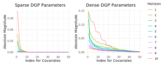
Figure 1: VAR(4) Parameter Coefficients for $h-$step ahead estimating equations

Notes. The parameters are from $p=100$ setting. Each line represents the absolute magnitude of the coefficients of control variables for each horizon’s estimating equations. The parameters are from the sparse and dense settings described in Section 3.

The local projection estimation equation is

$$y_{t+h}= \beta_{h}y_{t}+\sum_{k=1}^{K}\delta_{h,k}^{\prime}\bm{z}_{t-k}+u_{t,h},$$

where the parameters of interest are the reduced-form impulse responses $\beta_{h}$ for $h=1,\dots,h_{\max}$. I set the parameter setting as $T=500$ and $p=\{25,50,100\}$. I include $K=4$ lags for all three methods, which makes the number of controls other than the innovation variable in each equation $p\times K$. Denote this dimension as $\widetilde{p}=\{100,200,400\}$.

I compare the coverage probabilities and the median widths of the confidence intervals with $1000$ replications. I used the code provided by Stephan Angrick for the standard local projection estimations. For the debiased lasso estimation, I use the R package desla provided by Adamek et al. (2023b), as I find their paper the most recent lasso-based method.

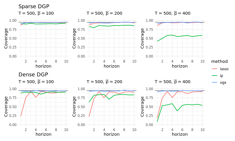
Figure 2: VAR, Dense DGP, $95\%$ Coverage Probabilities

Notes. The results are based on $1000$ iterations of sample size $T=500$ and the number of controls $\widetilde{p}=\{100,200,400\}$ from the VAR$(4)$ DGP described in section 3. The plots are coverage probabilities of reduced-form impulse responses at horizons from 1 to 10. Lag orders are set to be $4$ for all the methods.

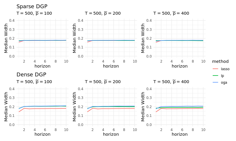
Figure 3: VAR, Dense DGP, Width of the Confidence Intervals

Notes. The median widths are calculated with $1000$ iterations of sample size $T=500$ and the number of controls $\widetilde{p}=\{100,200,400\}$ from the VAR$(4)$ DGP described in section 3. The plots are coverage probabilities of reduced-form impulse responses at horizons from 1 to 10. Lag orders are set to be $4$ for all the methods.

The results are shown in Figures 2 and 3. I excluded the results for the $0$ horizon case because they are set to be $1$ regardless of the estimating methods. The upper plots show the results obtained from the sparse DGP with smaller $\rho_{k}$ values. For the case where $\widetilde{p}=100$, all three methods perform well, although the standard local projection method slightly performs under par. As the dimensionality increases, the standard local projection fails considerably while both high-dimensional methods continue to achieve the desired $95\%$ coverage rates. It is worth noting that the results are not derived from the widths of the confidence intervals, as can be seen from Figure 3. The lower plots are the results from the dense DGP with higher $\rho_{k}$ values. In the relatively low-dimensional scenario, the standard local projection outperforms LASSO, but both fall short of the $95\%$ coverage rate. A similar pattern can be observed for the standard local projection: as the dimension increases, it fails noticeably. On the other hand, the proposed method, denoted OGA, performs equally well across all settings. The widths of the confidence intervals are also similar between standard lp and OGA, while LASSO has slightly smaller widths.

4 Theory

4.1 Preliminaries

In this subsection, I introduce the definitions used throughout the theory. Most of the definitions and explanations are taken from Davidson (2021). I will use these definitions in the context of the main text in the following subsection.

Consider a probability space $(\Omega,\mathcal{F},P)$. With time series data, time flows in one direction: The past is known while the future is unknown. It is hence important to condition on previous information set in the context of time series analysis. The accumulation of information is represented by an increasing sequence of sub $\sigma-$fields, $\{\mathcal{F}_{t}\}_{-\infty}^{\infty}$, where $\mathcal{F}_{s}\subseteq\mathcal{F}_{t}$ for $s\leq t$. With the uncertainty of the future, the natural next step is to take expectations. If $X_{t}$ is $\mathcal{F}_{t}-$measurable for each $t$, $\{X_{t},\mathcal{F}_{t}\}_{-\infty}^{\infty}$ is called an adapted sequence, and $E[X_{t}|\mathcal{F}_{t-1}]$ is defined. Also, if $E[X_{t+s}|\mathcal{F}_{t}]=X_{t}$ a.s. for all $s\geq 0$ under adaptation, the sequence is identified by its history alone, and $\{X_{t}\}_{-\infty}^{\infty}$ is called a causal stochastic sequence. I start by introducing the most widely used dependence concept, the martingale difference (m.d.) sequences.

Definition 1 (Martingale difference sequence, Davidson (2021)).

The process $\{X_{t}\}_{-\infty}^{\infty}$ is a martingale difference sequence if

$$E[X_{t}]< \infty$$

$$E[X_{t}|\mathcal{F}_{-\infty}^{t-1}]= 0\quad a.s.$$

As is clear from the definition, m.d. assumes one-step-ahead unpredictability. It follows that it is uncorrelated with any measurable function of its lagged values, and thus behaves like independent sequences in classical limit results. As shown in Davidson (2021), many limit theorems that hold under independence also hold under the m.d. assumption with few additional assumptions about the marginal distributions, making it a preferred dependence assumption for econometricians. To extend our understanding beyond one-step-ahead unpredictability, the next definition introduces the concept of asymptotic unpredictability.

Definition 2 (Mixingale, Davidson (2021)).

For $q\geq 1$, the sequence $\{X_{t},\mathcal{F}_{t}\}_{-\infty}^{\infty}$ is an $L_{q}-$mixingale if for a sequence of non-negative constants $\{c_{t}\}_{-\infty}^{\infty}$ and $\{\rho_{m}\}_{0}^{\infty}$ such that $\rho_{m}\to 0$ as $m\to\infty$,

$$\left(E\left[\left|E[X_{t}|\mathcal{F}_{-\infty}^{t-m}]\right|^{q}\right]\right)^{1/q}\leq c_{t}\rho_{m},$$ (4.1)

$$\left(E\left[\left|X_{t}-E[X_{t}|\mathcal{F}_{-\infty}^{t+m}]\right|^{q}\right]\right)^{1/q}\leq c_{t}\rho_{m+1},$$ (4.2)

hold for all $t$ and $m\geq 0$.

A mixingale generalizes a m.d. as a special case where $\rho_{m}=0$ for all $m>0$. The equations show a diminishing effect of past information on the present, while suggesting eventual complete knowledge of the present in the distant future. Note that if the sequence is adapted, then $E[X_{t}|F_{-\infty}^{t+m}]=X_{t}$ for all $m\geq 0$ and (4.2) is satisfied. Just as m.d.s behave like independent sequences in limit theorems, mixingales behave like mixing sequences, which implies asymptotic independence with the following definitions.

Definition 3 ($\alpha-$mixing coefficients, Hansen (1991)).

The $\alpha-$mixing coefficients of a sequence $\{X_{t}\}_{-\infty}^{\infty}$ are given by

$$\alpha_{m}=\sup_{j}\sup_{\{F\in\mathcal{F}_{-\infty}^{j},G\in\mathcal{F}_{j+m}^{\infty}\}}|P(G\cap F)-P(G)P(F)|,$$

and the process $X_{t}$ is said to be $\alpha-$mixing if $\lim_{m\to\infty}\alpha_{m}=0$.

The $\alpha-$mixing coefficient $\alpha_{m}$ measures the dependence between the sequences separated by a lag of $m$. If a process $X_{t}$ is $\alpha-$mixing, the dependence diminishes as the lag increases. Mixing conditions often play a crucial role in further establishing asymptotic properties. Although the mixingale condition offers several advantageous properties, an important limitation arises: even if a function of mixingales is independent, it loses its mixing property with an infinite number of lags (Davidson (2021), Chapter 18). The following definition introduces a mapping from a mixing process to a random sequence. This transformation enables the sequence to inherit some desired mixingale properties.

Definition 4 (Near Epoch Dependence (NED), Davidson (2021)).

For a stochastic process $\{V_{t}\}_{-\infty}^{\infty}$, let $\mathcal{F}_{t-m}^{t}=\sigma\{V_{t-m},\dots,V_{t}\}$, such that $\{\mathcal{F}_{t-m}^{t}\}_{m=0}^{\infty}$ is an increasing sequence of $\sigma-$fields. If for $q>0$ an adapted sequence $\{X_{t}\}_{-\infty}^{\infty}$ satisfies

$$\left(E\left[\left|X_{t}-E(X_{t}|\mathcal{F}_{t-m}^{t})\right|^{q}\right]\right)^{1/q}\leq d_{t}\zeta_{m},$$ (4.3)

where $\zeta_{m}\to 0$ as $m\to\infty$ and $\{d_{t}\}_{-\infty}^{\infty}$ is a sequence of positive constants, $X_{t}$ is said to be near-epoch dependent in $L_{q}-$norm ($L_{q}-$NED) on $\{V_{t}\}_{-\infty}^{\infty}$.

The NED condition is the main dependence assumption I use on the data, following Adamek et al. (2023a) and Adamek et al. (2023b). In the rest of the subsection, I introduce some useful lemmas using the aforementioned definitions.

The following lemma gives a concentration bound without a specific assumption on the dependence structure, which will be used both in Theorems 4.1 and 4.3.

Lemma 4.1 (Triplex inequality, Jiang (2009)).

Let $\{X_{t}\}_{-\infty}^{\infty}$ be a causal stochastic sequence and $\{\mathcal{F}_{t-m}^{t}\}_{m=0}^{\infty}$ be an increasing sequence of $\sigma-$fields. Let $\{X_{t}\}$ be $\mathcal{F}_{t}-$measurable for each $t$. Then for any $\epsilon,M>0$ and positive integers $m$,

$$\begin{split}P\left(\left|{1\over T}\sum_{t=1}^{T}X_{t}-EX_{t}\right|>\epsilon\right)&\leq 2m\exp{\left(-{T\epsilon^{2}\over 288m^{2}M^{2}}\right)}\\ &+(6/\epsilon){1\over T}\sum_{t=1}^{T}E[E[X_{t}|\mathcal{F}_{t-m}]-EX_{t}]\\ &+(15/\epsilon){1\over T}\sum_{t=1}^{T}E\big{[}|X_{t}|\,\mathbbm{1}\{|X_{t}|>M\}\big{]}\end{split}$$ (4.4)

This inequality is called the triplex inequality because it has three components. The first element is a Bernstein-type bound, the second deals with dependence, and the last component is on the tail. This bound is a central theory used in the proofs, where I use the mixingale property inherited by the NED assumption to simplify the dependence and the tail bounds. The following lemma provides the simplified bounds by imposing the mixingale assumptions on $\{X_{t}\}_{-\infty}^{\infty}$.

Lemma 4.2 (Triplex inequality for mixingales).

Suppose the assumptions in Lemma 4.1 hold. Further assume that the moment generating function for $X_{t}$ exists and $\{X_{t}\}_{-\infty}^{\infty}$ is an $L_{\bar{q}-}$bounded $L_{q}-$mixingale with constants $c_{t}$ and $\rho_{m}\to 0$ for some $1\leq\bar{q}\leq q$, so that $E[|X_{t}|^{\bar{q}}]\leq C$.Then for any $\epsilon,M>0$ and positive integers $m$,

$$\begin{split}P\left(\left|{1\over T}\sum_{t=1}^{T}X_{t}-EX_{t}\right|>\epsilon\right)&\leq 2m\exp{\left(-{T\epsilon^{2}\over 288m^{2}M^{2}}\right)}\\ &+{6\overline{c}_{T}\over\epsilon}\rho_{m}+{15\over\epsilon}C\exp(-M(\bar{q}-1)),\end{split}$$ (4.5)

where $\overline{c}_{T}:=\sum_{t=1}^{T}c_{t}/T$.

Proof.

The proof can be found in Appendix B.1. ∎

4.2 Assumptions and Lemmas

The definitions of the variables and the parameters come from the baseline models (2.1) – (2.3). I start by introducing the assumptions on the data generating processes.

Assumption 1 (NED).

Denote $\epsilon_{t,h}$ as a genereric notation for the error terms $u_{t,h},e_{t,h},$ and $v_{t,h}$. There exist some constants $\bar{q}>q>2$, and $b\geq\max\{1,(\bar{q}/q-1)/(\bar{q}-2)\}$ such that

1. $(x_{t},\bm{w}_{t},u_{t,h},e_{t,h})$ are zero-mean causal stochastic process with $E[x_{t}u_{t,h}]=E[x_{t}e_{t,h}]=0$ and $E[\bm{w}_{t}u_{t,h}]=E[\bm{w}_{t}e_{t,h}]=\bm{0}$.

2. $\max_{1\leq j\leq p}E[|w_{t,j}|^{2\bar{q}}]\leq C$ and $\max_{1\leq h\leq H_{\max}}E[|\epsilon_{t,h}|^{2\bar{q}}]\leq C$.

3. Denote the moment generating function of $X$ as $M_{X}(t)$. Assume $M_{X}(t)<\infty$ for $X=\{w_{t,j}\epsilon_{t,h},w_{t,j}w_{t,k}\}$ for all $j,k=1,\dots,p,j\neq k$.

4. Let $\{\Upsilon_{T,t}\}$ denote a triangular array that is $\alpha-$mixing of size $-b/(1/q-1/\bar{q})$ with $\sigma-$field $\mathcal{F}_{t}^{\Upsilon}:=\sigma\{\Upsilon_{T,t},\Upsilon_{T,t-1},\dots\}$ such that $(x_{t},\bm{w}_{t},u_{t,h},e_{t,h})$ is $\mathcal{F}_{t}^{\Upsilon}-$measurable. The processes $x_{t}$, $w_{t,j}$, $u_{t,h}$, and $e_{t,h}$ are $L_{2q}-$near-epoch-dependent (NED) of size $-b$ on $\Upsilon_{T,t}$ with positive constants $\{d_{t}\}$ and a sequence $\zeta_{m}\to 0$ as $m\to\infty$, uniformly over $j=1,\dots,p$.

Assumption 1 (a) assumes that the error terms in (2.1) and (2.2) are not correlated with the contemporaneous regressors. Note that I impose the adaptation assumption to use asymptotic martingale difference property the Bernstein blocks must have (Davidson (1994), page 387). According to Davidson (2021), it is a widely employed assumption in time series econometrics, assuming that future shock information cannot help in predicting $X_{t}$ given its history (Davidson (2021), page 383). Assumption 1 (b) ensures the processes have bounded $2\bar{q}-$th moments. Assumption 1 (d) is on the dependence structure. While $(x_{t},\bm{w}_{t},u_{t,h},e_{t,h})$ themselves are not mixing processes, they depend almost entirely on ‘near epoch’ of $\{\Upsilon_{t}\}$ (Davidson (2021), page 368), which is $\alpha-$mixing. This allows $(x_{t},\bm{w}_{t},u_{t},e_{t,h})$ to inherit some mixingale properties, as will be stated in the following lemma.

Lemma 4.3 (Mixingale Property).

Denote $\epsilon_{t,h}$ as a genereric notation for the error terms $u_{t,h},e_{t,h},$ and $v_{t,h}$. Under Assumption 1, the following holds. Note that $\{c_{t}\}$ and $\rho_{m}$ are generic notations for the mixingale constants.

1. $\{v_{t,h}\}_{t=-\infty}^{\infty}$ is causal $L_{2q}-$NED of size $-b$ on $\Upsilon_{T,t}$ with positive bounded constants uniformly over $h=1,\dots,H_{\max}$.

2. $\{w_{t,j}\epsilon_{t}\}$ is a causal $L_{q}-$mixingale with non-negative constants $\{c_{t}\}$ and sequences $\rho_{m}$ for all $j=1,\dots,p$ and $h=1,\dots,H_{\max}$.

3. $\{w_{t,j}w_{t,k}-E[w_{t,j}w_{t,k}]\}$ is a causal $L_{q}-$mixingale with non-negative constants $\{c_{t}\}$ and sequences $\rho_{m}$ for all $j\neq k$ where $j,k=1,\dots,p$.

Proof.

The proof can be found in Appendix B.2. ∎

This lemma shows that some transformations of NEDs and their demeaned processes are mixingales. It thus allows us to use Lemma 4.2. Next, I impose some assumptions on the mixingale constants to simplify some bounds used in the proof of the main theorems.

Assumption 2.

Recall the NED constants $\{d_{t}\}$ and a sequence $\zeta_{m}\to 0$ defined in Assumption 1 (d). Let $\widetilde{\zeta}_{m}=2\zeta_{m}+\zeta_{m}^{2}$ and $k:=[q/2]$. Define $\rho_{m}=6\alpha_{k}^{1/q-1/\bar{q}}+2\widetilde{\zeta}_{k}$, where $\alpha_{k}$ is the mixing coefficient for the sequences $X=\{\epsilon_{t,h},v_{t,h},w_{t,j}\epsilon_{t,h},w_{t,j}w_{t,k}\}$ for all $j=1,\dots,p$ and $h=1,\dots,H_{\max}$. Assume that

$$\rho_{m}\leq\exp(-m\kappa)$$

for some $\kappa>c_{\kappa}\log p$, where $c_{\kappa}>2$.

This assumption is on the mixingale constants, where I define the constants to align with the constants that inherit the mixingale properties. The sequence $\rho_{m}\to 0$ is hence the mixingale sequence for the transformed variables in Lemma 4.3. Assumption 2 gives the assumption of how fast $\rho_{m}$ should decay. The parameter $\kappa$ governs the strength of the dependence, with larger $\kappa$ values indicating a weaker dependence. Note that this is a technical assumption I need to prove Thoerem 4.1, where it simplifies the dependence bound in the triplex inequality (4.4). The following is the assumptions on the degree of sparseness of the underlying coefficients, $\lambda_{h}$ and $\gamma_{h}$.

Assumption 3.

Let $|\beta_{h}|\leq C$. Let $\xi$ be a generic notation that represents $\beta_{-h}$, $\lambda_{h}$, and $\gamma_{h}$ for all $h=1,\dots,H_{\max}$. Then $\xi$ follows the following assumption. Suppose $\sum_{j=1}^{p}\xi_{j}^{2}\leq C$. Also assume that there exists $\delta>1$ and $0<C_{\delta}<\infty$ that for any $J\subseteq\mathfrak{P}$,

$$\sum_{j\in J}\left|\xi_{j}\right|\leq C_{\delta}\left(\sum_{j\in J}\xi_{j}^{2}\right)^{(\delta-1)/(2\delta-1)},$$ (4.6)

where $C$ refers to a generic constant $0<C<\infty$. $\mathfrak{P}$ refers to the power set of $J$, where $J$ is a set of covariates.

This assumption is the main difference between this method and LASSO, in that it doesn’t limit the number of nonzero coefficients, but rather restricts the magnitudes of the coefficients. While we do not require that the parameters to have a natural order, these conditions can be expressed more simply by rearranging the parameters in descending order of their magnitude $|\xi_{j}|$. Denote the rearrangement as $|\xi_{(1)}|\geq|\xi_{(2)}|\geq\dots\geq|\xi_{(p)}|$. Then, Assumption 3 3 implies

$$C_{1}j^{-\delta}\leq\left|\xi_{(j)}\right|\leq C_{2}j^{-\delta},\>0<C_{1}\leq C_{2}<\infty,\>\delta>1,$$ (4.7)

where from (4.7) we call Assumption 3 3 as a polynomial decay case: if (4.7) holds for some $\delta>1$, then (4.6) holds for the same $\delta$, as shown in Lemma A.2 in Ing (2020). Apart from (4.7), it can be shown that Assumption 3 3 also implies

$$\sum_{j=1}^{p}\left|\xi_{j}\right|^{1/\delta}<C,\>0<C<\infty,\>\delta>1,$$ (4.8)

which is a frequently adopted assumption in the high-dimensional literature, as in Wang et al. (2014). Assume that (4.8) holds for some $\delta$. Applying Hölder’s inequality,

$$\sum_{j\in J}\left|\xi_{j}\right|\leq \left(\sum_{j\in J}\left|\xi_{j}\right|^{{1\over 2\delta-1}{2\delta-1\over\delta}}\right)^{\delta/(2\delta-1)}\left(\sum_{j\in J}\xi_{j}^{{2\delta-2\over 2\delta-1}{2\delta-1\over\delta-1}}\right)^{(\delta-1)/(2\delta-1)}$$

$$= \left(\sum_{j\in J}\left|\xi_{j}\right|^{1/\delta}\right)^{\delta/(2\delta-1)}\left(\sum_{j\in J}\xi_{j}^{2}\right)^{(\delta-1)/(2\delta-1)}$$

$$\leq C^{\delta/(2\delta-1)}\left(\sum_{j\in J}\xi_{j}^{2}\right)^{(\delta-1)/(2\delta-1)},$$

and we can see that by setting $C_{\delta}=C^{\delta/(2\delta-1)}$, (4.6) holds. The parameter $\delta$ governs the degree of sparseness, with larger values indicating a faster decay of the coefficients. Thus, we can see that Assumption 3 covers a wider class of sparsity conditions where the condition trivially implies the exact sparsity case.

Remark.

There are many variations of sparsity-based assumptions that extend the exact/strong sparse assumption. First, (4.8) is called a soft sparsity, as opposed to strong sparsity, in that $L_{q}$ norm is bounded for $0<q\leq 1$, whereas strong sparsity means that $L_{0}$ norm is bounded by a small constant. Another concept is the approximate sparsity (Chernozhukov et al. (2021), Comment 3.1). The concept is to add a fast enough approximation error based on the error bounds, so that exact sparsity can “approximate” a less sparse DGP such as (4.7).

Assumption 4.

Assume the followings.

1. For some positive constant $C_{1}$ and $C_{2}$, it holds that

   $$\max_{1\leq|J|\leq C_{1}(T/\log p)^{1/2},i\notin J}\left\lVert\Gamma^{-1}(J)E[w_{t,i}\bm{w}_{t}(J)]\right\rVert_{1}<C_{2},$$

   where $\Gamma(J)=E[\bm{w}_{t}(J)\bm{w}_{t}(J)^{\prime}]$.

2. Let $\Sigma=E[\sum_{t=1}^{T}\bm{w}_{t}\bm{w}_{t}^{\prime}/T]$. Assume $\max_{j\in[p]}\Sigma_{j,j}<C$ and $1/C\leq\Lambda_{\min}$, where $\Lambda_{\min}$ is the minimum eigenvalue of $\Sigma$ and $0<C<\infty$.

3. $\log p=o(T^{{\delta-1\over 3(2\delta-1)}})$ and $(T/(\log p)^{3})^{1/2}p^{-\underline{c}}=o(1)$ for some $\underline{c}=\min\{c_{\kappa}-2,c_{M}(\bar{q}-1)-2\}>0$, where $c_{M}>2/(\bar{q}-1)$ and $c_{\kappa}>2$.

Assumption 4 are some additional assumptions on the covariates and growth rates of the dimensionality $dim(\bm{w}_{t})=p$. Assumption 4 (a) limits strong correlations between covariates, ensuring that the OLS coefficients of one covariate on any set of other covariates remain finite. Assumption 4 (b) is on minimum eigenvalue of the Gram matrix, with a remark that this condition is on the population level, not on the sample matrix as in the restricted eigenvalue conditions in Bickel et al. (2009). The third condition addresses the relationship between the growth of the covariate dimension $p$ and sample size $T$. It specifies that $\log p$ should not grow too quickly compared to $T$. This condition is crucial for bounding the triplex inequality in the proof of Theorem 4.1. Note that this assumption is stronger than the usual growth rates in the high-dimensional literature with i.i.d. data, for example $\log p=o(T^{1/3})$ in Belloni et al. (2013). While bounding either the Bernstein bound or the tail bound would require $\log p=o(T^{(\delta-1)/(2\delta-1)})$, bounding all the terms simultaneously requires a stricter condition $(\log p)^{3}=o(T^{(\delta-1)/(2\delta-1)})$. More detailed explanations are given in the proofs of Theorems 4.1 and 4.2. While this may sound restrictive, note that this assumption is on the growth rate of $\log p$, where $p$ can grow at much faster rates.

4.3 Inference

In this subsection I establish the inference for the parameter of interest with each horizon $h$. I use a matrix representation as the baseline instead of (2.1) – (2.3) for simplicity. Let $\bm{y}_{h}$, $\bm{x}_{h}$, $\bm{u}_{h}$, and $\bm{v}_{h}$ be the $T\times 1$ vector and $W_{h}$ be the $T\times p$ matrix, where $p=dim(\bm{w}_{t})$. Then the models can be written in a compact matrix form:

$$\begin{split}\bm{y}_{h}=&\beta_{h}\bm{x}_{h}+W_{h}\beta_{-h}+\bm{u}_{h},\\ \bm{x}_{h}=&W_{h}\gamma_{h}+\bm{v}_{h}.\end{split}$$ (4.9)

Theorem 4.1 (Error bounds for Double OGA+HDAIC).

Denote $\xi$ as a representative vector of parameters, $\beta_{-h}$ and $\gamma_{h}$, for all $h=1,\dots,H_{\max}$. Denote $E_{T}[.]=E[.|(y_{t+h},x_{t},\bm{w}_{t})_{t=1}^{T-h}]$. Under Assumptions 1 – 4, the following holds for all $h=1,\dots,H_{\max}$.

$$E_{T}\left[\left\lVert W_{h}(\widehat{\xi}-\xi)\right\rVert^{2}\right]=O_{p}\left(\left({(\log p)^{3}\over T}\right)^{1-1/2\delta}\right).$$ (4.10)

Proof.

The proof can be found in Appendix A.1. ∎

Note that the convergence rates are not the fastest rates proposed in the main theorem in Ing (2020): the error bounds are $(\log p/T)^{1-1/2\delta}$ for the polynomial decay case. The main results require assumptions (A1) and (A2) in Ing (2020), and with Assumption 1 and Lemma 4.2 those assumptions are not satisfied. I hence use the bounds from weakened assumptions in equations (2.33) and (2.34) in Ing (2020), resulting in the slower converge rates. As noted in equation (2.35) of Ing (2020), these relaxed assumptions require $\log p=o(T^{1/3}),$ which is implied by Assumption 4 (c). While Theorem 4.1 itself is useful in deriving error bounds for the high-dimensional nuisance parameters, our parameter of interest is ${\beta}_{h}$ in equation (2.1). The following theorem derives asymptotic distribution of $\widehat{\beta}_{h}$ using the error bounds derived in Theorem 4.1.

Theorem 4.2.

Under Assumptions 1 – 4,

$$\sqrt{T}(\widehat{\beta}_{h}-\beta_{h})\overset{d}{\to}N(0,\sigma_{h}^{2}),$$

where $\sigma_{h}^{2}=\lim_{T\to\infty}\Omega_{h}/\tau_{h}^{4}$, $\Omega_{h}$ is the long-run covariance matrix following Newey-West, and $\tau^{2}=E[\bm{v}_{h}^{\prime}\bm{v}_{h}/T]$.

Proof.

The proof can be found in Appendix A.2. ∎

By Theorem 4.2, the estimator of interest achieves the square root $T$ convergence rate regardless of the slower convergence rate of the nuisance parameters presented in Theorem 4.1. The following theorem establishes the validity of the proposed variance estimator.

Theorem 4.3.

Define $\psi_{h,t}=v_{h,t}u_{t}$ and $\tau_{h}^{2}=E[\bm{v}_{h}\bm{v}_{h}/T]$. Let $\sigma_{h}^{2}=\lim_{T\to\infty}\tau_{h}^{-4}\Omega_{h}$, where $\Omega_{h}=\sum_{\ell=-(T-1)}^{T-1}1/T\sum_{t=\ell+1}^{T}E[\psi_{h,t}\psi_{h,t-\ell}]$ with a bandwidth parameter $K$. Denote the sample analogues as $\hat{\tau}_{h}$, $\hat{\sigma}_{h}^{2}$ and $\hat{\Omega}_{h}$. Under Assumptions 1 – 4,

$$\left|\hat{\sigma}_{h}^{2}-\sigma_{h}^{2}\right|\overset{p}{\to}0.$$

Proof.

The proof can be found in Appendix A.3. ∎

With Theorems 4.2 and 4.3, we can now construct $100(1-\alpha)\%$ confidence intervals for each horizon. Given a confidence level $\alpha$, an asymptotic $100(1-\alpha)\%$ confidence interval $\widehat{\mathcal{I}}_{\alpha,h}$ is given by

$$\widehat{\mathcal{I}}_{\alpha,h}:=[\widehat{\beta}_{h}-z_{\alpha}\hat{\sigma}_{h}/\sqrt{T},\>\>\widehat{\beta}_{h}+z_{\alpha}\hat{\sigma}_{h}/\sqrt{T}],$$ (4.11)

where $z_{\alpha}=\Phi^{-1}(1-\alpha/2)$ is the $(1-\alpha/2)$ quantile of the standard normal distribution and $\hat{\sigma}_{h}$ is defined in Theorem 4.2.

5 Concluding Remarks

Local projection has emerged as the preferred alternative to VARs in impulse response analysis due to its robustness to model misspecification and ease of implementation. As its popularity has grown, a burgeoning literature has explored the robustness and interpretability of local projection estimators, echoing the findings of studies such as Montiel Olea and Plagborg-Møller (2021) and Angrist et al. (2018b).

With increasing data availability, it is natural to include more and more controls to control for possible unobserved covariates, especially to support the conditional independence assumption as in Angrist et al. (2018b). Considering the lag augmentations (Montiel Olea and Plagborg-Møller (2021)), the number of covariates naturally grows faster. These considerations lead to high-dimensional time series linear regression models. However, the existing methods, especially those based on LASSO, have been criticized by Giannone et al. (2021) and Kolesár et al. (2023) with the challenge of verifying the sparsity assumptions in the underlying DGP. In particular, Giannone et al. (2021) showed the potential dense DGPs in empirical examples, including macroeconomic scenarios.

This paper aims to address the gap in the literature by introducing a high-dimensional local projection approach that caters to both sparse and dense settings and takes into account the uncertainty of sparseness in the DGP. By utilizing the OGA with HDAIC method proposed by Ing (2020) and the NED assumptions, the local projection estimator achieves $\sqrt{T}$ asymptotic normality with HAC standard errors. The theoretical foundation of this method is based on the error bounds of Ing (2020), the triplex inequality of Jiang (2009), and double selection arguments of Belloni et al. (2013).

In addition, our approach has the advantage of interpretability through the use of OGA, which orders covariates based on their explanatory power. Following the arguments in Ing (2020), I demonstrate that our assumption on the parameters includes the conventional extensions of sparsity-based assumptions, which distinguishes our method and makes it a robust solution for both sparse and dense DGPs. This paper contributes to the field of high-dimensional time series methods by providing a flexible and interpretable approach to local projection estimation.

Appendix A Proof of Main Theorems

Notations.

For a vector $X=(X_{1},\dots,X_{p})^{\prime}$, $||X||_{q}=(\sum_{j=1}^{p}X_{j}^{q})^{1/q}$ denotes the L-$q$ norm for $q<\infty$ and $||X||_{\infty}=\max_{1\leq j\leq p}|X_{j}|$.

A.1 Proof of Theorem 4.1

Proof.

The main purpose of this proof is to show that the assumptions (2.33) and (2.34) in Ing (2020) hold under Assumptions 1 – 4. Since the estimating equations are (2.2) and (2.3), the assumptions should hold on the two equations.

I start with condition (2.34) in Ing (2020) because it is a stringent condition than (2.33). It states that there exists a constant $c>0$ such that

$$P\left(\max_{1\leq j,k\leq p,j\neq k}\left|{1\over T}\sum_{t=1}^{T}w_{t,j}w_{t,k}-E[w_{t,j}w_{t,k}]\right|\geq c\sqrt{{(\log p)^{3}\over T}}\right)=o(1).$$ (A.1)

For any $x\geq 0$, it follows from the union bound that

$$P \left(\max_{1\leq j,k\leq p,j\neq k}\left|{1\over T}\sum_{t=1}^{T}w_{t,j}w_{t,k}-E[w_{t,j}w_{t,k}]\right|\geq x\right)$$

$$\qquad\qquad\leq\sum_{j=1}^{p}\sum_{k=1}^{p}P\left(\left|{1\over T}\sum_{t=1}^{T}w_{t,j}w_{t,k}-E[w_{t,j}w_{t,k}]\right|\geq x\right)$$

$$\qquad\qquad\leq p^{2}\,P\left(\left|{1\over T}\sum_{t=1}^{T}w_{t,j}w_{t,k}-E[w_{t,j}w_{t,k}]\right|\geq x\right).$$

Notice that by Lemma 4.3 (c), we can apply the triplex inequality Lemma 4.2,

$$p^{2}\,P \left(\left|{1\over T}\sum_{t=1}^{T}w_{t,j}w_{t,k}-E[w_{t,j}w_{t,k}]\right|\geq x\right)$$

$$\leq \>\>2p^{2}m\exp{\left(-{Tx^{2}\over 288m^{2}M^{2}}\right)}$$ (BD1)

$$+{6\overline{c}_{T}\over x}p^{2}\rho_{m}$$ (BD2)

$$+{15C\over x}p^{2}\exp(-M(\bar{q}-1)),$$ (BD3)

where $m$ is a positive integer number and $M>0$ is some constant. I proceed by showing that there is a sequence $\eta_{T}\to 0$ as $T\to\infty$ that bounds all the components (BD1) – (BD3). Since Lemma 4.2 holds for all positive integer $m$ and a constant $M>0$, the bounds can be further simplified by defining $m$ and $M$ in terms of $T$ and $p$ (Jiang (2009), Remark 2). Let $M=c_{M}\log p$ and $m=1$, where $c_{M}>2/(\bar{q}-1)$. To match the convergence rate in (A.1), let $x=c_{1}((\log p)^{3}/T)^{1/2}$, where $c_{1}>24c_{M}$. By Assumption 2, $\rho_{m}\leq\exp(-c_{\kappa}\log p)$, and the bounds become

$$P \left(\max_{1\leq j,k\leq p,j\neq k}\left|{1\over T}\sum_{t=1}^{T}w_{t,j}w_{t,k}-E[w_{t,j}w_{t,k}]\right|\geq x\right)$$

$$\leq \>\>Cp^{2}\exp\left(-{c_{1}^{2}\over 288c_{M}^{2}}\log p\right)$$

$$+Cx^{-1}p^{2}\exp\left(-c_{\kappa}\log p\right)$$

$$+Cx^{-1}p^{2}\exp(-c_{M}(\bar{q}-1)\log p),$$

where I abuse the notation $C$ for a generic constant, because only the constants inside the exponential terms matter. The first term is $o(1)$ if $c_{1}^{2}/(288c_{M}^{2})>2$, which is satisfied by setting $c_{1}>24c_{M}$. Similarly, the second and the third term are $o(1)$ if $c_{\kappa}>2$ and $c_{M}(\bar{q}-1)>2$, which is satisfied by definitions of the constants. Therefore, all terms are $o(1)$ and hence equation A.1 is satisfied.

Next we turn to condition (2.32) in Ing (2020). It states that there exists a constant $c>0$ such that

$$P\left(\max_{1\leq j\leq p}\left|{1\over T}\sum_{t=1}^{T}w_{t,j}e_{t,h}\right|\geq c\sqrt{{(\log p)^{3}\over T}}\right)=o(1)$$ (A.2)

and

$$P\left(\max_{1\leq j\leq p}\left|{1\over T}\sum_{t=1}^{T}w_{t,j}v_{t,h}\right|\geq c\sqrt{{(\log p)^{3}\over T}}\right)=o(1),$$ (A.3)

for all $h=1,\dots,H_{\max}$.

Consider the case with $\{w_{t,j}e_{t,h}\}$. Applying the union bound, for any $x\geq 0$ it holds that

$$P \left(\max_{1\leq j\leq p}\left|{1\over T}\sum_{t=1}^{T}w_{t,j}e_{t,h}-E[w_{t,j}e_{t,h}]\right|\geq x\right)$$

$$\qquad\qquad\leq\sum_{j=1}^{p}P\left(\left|{1\over T}\sum_{t=1}^{T}w_{t,j}e_{t,h}-E[w_{t,j}e_{t,h}]\right|\geq x\right)$$

$$\qquad\qquad\leq p\,P\left(\left|{1\over T}\sum_{t=1}^{T}w_{t,j}e_{t,h}-E[w_{t,j}e_{t,h}]\right|\geq x\right).$$

By Assumption 2 2 and Lemma 4.3 (b), we can apply Lemma 4.2, and

$$p\,P \left(\left|{1\over T}\sum_{t=1}^{T}w_{t,j}e_{t,h}-E[w_{t,j}e_{t,h}]\right|\geq x\right)$$

$$\leq \>\>Cp\exp\left(-{c_{1}^{2}\over 288c_{M}^{2}}\log p\right)$$

$$+Cx^{-1}p\exp\left(-c_{\kappa}\log p\right)$$

$$+Cx^{-1}p\exp(-c_{M}(\bar{q}-1)\log p),$$

where all three terms are bounded by $\eta_{T}\to 0$ used to bound (BD1) – (BD3) since the above right hand side terms grow at a slower rate, by $p^{-1}$. Therefore, (A.2) holds.

The same argument applies for $\{w_{t,j}v_{t,h}\}$ case, because Assumption 2 2 and Lemma 4.3 applies analogously with same constants $\{c_{t}\}$ and $\rho_{m}$. By Lemma 4.2, all three terms are bounded by the same $\eta_{T}\to 0$, and hence (A.3) holds.

Assumptions (A3) in Ing (2020) are assumed in Assumption 3 and Assumption (A5) in Ing (2020) is assumed in Assumption 4 (a). This set of assumptions collectively satisfies the necessary conditions outlined in Theorem 3.1 of Ing (2020), thereby yielding the desired results. ∎

A.2 Proof of Theorem 4.2

Proof.

In this proof, I use notations in (4.9). Further, write (4.9) as

$$\begin{split}\bm{y}_{h}=&\beta_{h}\bm{x}_{h}+W_{h}\beta_{-h}+\bm{u}_{h}=:\beta_{h}\bm{x}_{h}+\mathfrak{g}+\bm{u}_{h},\\ \bm{x}_{h}=&W_{h}\gamma_{h}+\bm{v}_{h}=:\mathfrak{m}+\bm{v}_{h},\end{split}$$ (A.4)

where $\mathfrak{g}$ and $\mathfrak{m}$ are functions of $W_{h}$. In the following proof, I first show the probability limit of $\sqrt{T}(\widehat{\beta}_{h}-\beta)$ using similar arguments in Belloni et al. (2013) and then derive asymptotic distribution of it using Theorem 25.12 in Davidson (2021).

Recall the subset of the covariates notation $W_{h}(J)=(W_{h,j})_{j\in J}$ and denote $\widehat{\Sigma}(J)=W_{h}(J)^{\prime}W_{h}(J)/T$. Define

$$\sqrt{T}(\widehat{\beta}_{h}-\beta) =(\bm{x}_{h}^{\prime}M\bm{x}_{h}/T)^{-1}(\bm{x}_{h}^{\prime}M(\mathfrak{g}+\bm{u}_{h})/\sqrt{T})$$

$$=:A^{-1}B,$$

where $M_{J}:=I-P_{J}$ and $P_{J}=W_{h}({J})(W_{h}({J})^{\prime}W_{h}({J}))^{-1}W_{h}({J})^{\prime}$. Define $\widetilde{J}=\widehat{J}_{x}\cup\widehat{J}_{y}$, where $\widehat{J}_{x}$ and $\widehat{J}_{y}$ are the chosen covariates from the steps 1 and 2 in Algorithm 1. Also, let $\widetilde{\gamma}_{h}$ the projection coefficient of $\bm{x}_{h}$ onto span $W_{h}(\widetilde{J})$ and let $\widetilde{\alpha}_{h}$ be the projection coefficient of $\bm{v}_{h}$ onto span $W_{h}(\widetilde{J})$, respectively.

I will proceed by showing that

$$A=\bm{v}_{h}^{\prime}\bm{v}_{h}/T+o_{p}(1), B=\bm{v}_{h}^{\prime}\bm{u}_{h}/\sqrt{T}+o_{p}(1).$$

Decompose $A$ and $B$ into pieces using (A.4).

$$A= (\bm{x}_{h}^{\prime}M_{\widetilde{J}}\bm{x}_{h})/T$$

$$= (\mathfrak{m}+\bm{v}_{h})^{\prime}M_{\widetilde{J}}(\mathfrak{m}+\bm{v}_{h})/T$$

$$= \mathfrak{m}^{\prime}M_{\widetilde{J}}\mathfrak{m}/T+2\mathfrak{m}^{\prime}M_{\widetilde{J}}\bm{v}_{h}/T+\bm{v}_{h}^{\prime}\bm{v}_{h}/T-\bm{v}_{h}^{\prime}P_{\widetilde{J}}\bm{v}_{h}/T,$$

$$B= \bm{x}_{h}^{\prime}M_{\widetilde{J}}(\mathfrak{g}+\bm{u}_{h})/\sqrt{T}$$

$$= (\mathfrak{m}+\bm{v}_{h})^{\prime}M_{\widetilde{J}}(\mathfrak{g}+\bm{u}_{h})/\sqrt{T}$$

$$= \mathfrak{m}^{\prime}M_{\widetilde{J}}\mathfrak{g}/\sqrt{T}+\mathfrak{m}^{\prime}M_{\widetilde{J}}\bm{u}_{h}/\sqrt{T}+\bm{v}_{h}^{\prime}M_{\widetilde{J}}\mathfrak{g}/\sqrt{T}+\bm{v}_{h}^{\prime}\bm{u}_{h}/\sqrt{T}-\bm{v}_{h}^{\prime}P_{\widetilde{J}}\bm{u}_{h}/\sqrt{T}.$$

Notice that the pieces in $A$ and $B$ can be bounded similarly, except the bounds in $B$ should be more restrictive. Each piece in $A$ and $B$ can be then decomposed into components, using idempotent property of the orthogonal projection matrix $M$. Below are the components used as ingredients for bounding $A$ and $B$.

1. Bounds for $\left\lVert W_{h}^{\prime}\bm{v}_{h}/T\right\rVert_{\infty}$ and $\left\lVert W_{h}^{\prime}\bm{u}_{h}/T\right\rVert_{\infty}$
   From the proof of Theorem 4.1, (A.2) and (A.3) holds, and hence

   $$\left\lVert W_{h}^{\prime}\bm{v}_{h}/T\right\rVert_{\infty}=O_{p}\left(\left((\log p)^{3}/T\right)^{1/2}\right),$$ (A.5)

   and the same argument applies to $\left\lVert W_{h}^{\prime}\bm{u}_{h}/T\right\rVert_{\infty}$ because $e_{t,h}$ and $u_{t,h}$ share the same assumption in Assumption 1.

2. Bounds for $\left\lVert\widetilde{\gamma}_{h}-\gamma_{h}\right\rVert$ and $\left\lVert\widehat{\beta}_{-h}-\beta_{-h}\right\rVert$
   Recall from Assumption 4 (b) and Theorem 4.1 we have

   $$\left\lVert\widehat{\gamma}_{h}-\gamma_{h}\right\rVert \leq\left(\Lambda_{\min}^{-1}E_{T}\left[{1\over T}\sum_{t=1}^{T}\left((\widehat{\gamma}_{h}-\gamma_{h})^{\prime}\bm{w}_{t}\right)^{2}\right]\right)^{1/2}$$

   $$=O_{p}\left(\left({(\log p)^{3}\over T}\right)^{(2\delta-1)/(4\delta)}\right).$$

   Similarly,

   $$\left\lVert\widehat{\beta}_{-h}-\beta_{-h}\right\rVert \leq\left(\Lambda_{\min}^{-1}E_{T}\left[{1\over T}\sum_{t=1}^{T}\left((\widehat{\beta}_{-h}-\beta_{-h})^{\prime}\bm{w}_{t}\right)^{2}\right]\right)^{1/2}$$

   $$\leq\left(\Lambda_{\min}^{-1}E_{T}\left[{1\over T}\sum_{t=1}^{T}\left((\widehat{\lambda}_{h}-\lambda_{h})^{\prime}\bm{w}_{t}\right)^{2}\right]\right)$$

   $$=O_{p}\left(\left({(\log p)^{3}\over T}\right)^{(2\delta-1)/(4\delta)}\right),$$

   where the first inequality comes from Assumption 4 (b), the second from $\widetilde{J}\subset\widehat{J}_{y}$, and the third from Theorem 4.1.

3. Bounds for $\left\lVert M_{\widetilde{J}}\mathfrak{m}/\sqrt{T}\right\rVert$ and $\left\lVert M_{\widetilde{J}}\mathfrak{g}/\sqrt{T}\right\rVert$
   It follows from the definition of $M_{\widetilde{J}}$ and $\widetilde{\gamma}_{h}$ that $M_{\widetilde{J}}\mathfrak{m}=(I-P_{\widetilde{J}})W_{h}\gamma_{h}=W_{h}(\gamma_{h}-\widetilde{\gamma}_{h})$ and hence

   $$\begin{split}\left\lVert M_{\widetilde{J}}\mathfrak{m}/\sqrt{T}\right\rVert&\leq\left\lVert W_{h}(\widetilde{\gamma}_{h}-\gamma_{h})/\sqrt{T}\right\rVert\\ &=O_{p}\left(\left({(\log p)^{3}\over T}\right)^{(2\delta-1)/(4\delta)}\right)\end{split}$$ (A.6)

   from Theorem 4.1. For $\left\lVert M_{\widetilde{J}}\mathfrak{g}/\sqrt{T}\right\rVert$, it holds by equation (A.4) and triangle inequality that

   $$\left\lVert M_{\widehat{J}_{y}}\bm{y}_{h}/\sqrt{T}\right\rVert \geq\left\lVert M_{\widetilde{J}}(\beta_{h}\bm{x}_{h}+\mathfrak{g})/\sqrt{T}\right\rVert$$

   $$\geq\left\lVert\beta_{h}\right\rVert\left\lVert M_{\widetilde{J}}\bm{x}_{h}/\sqrt{T}\right\rVert-\left\lVert M_{\widetilde{J}}\mathfrak{g}/\sqrt{T}\right\rVert,$$

   where $\left\lVert\beta_{h}\right\rVert\leq C$ by Assumption 3. Since $\left\lVert M_{\widehat{J}_{y}}\bm{y}_{h}/\sqrt{T}\right\rVert$ and $\left\lVert M_{\widetilde{J}}\right\rVert\bm{x}_{h}/\sqrt{T}$ share the same error bound by Theorem 4.1,

   $$\left\lVert M_{\widetilde{J}}\mathfrak{g}/\sqrt{T}\right\rVert=O_{p}\left(\left({(\log p)^{3}\over T}\right)^{(2\delta-1)/(4\delta)}\right).$$

4. Bounds for $\left\lVert\widetilde{\gamma}_{h}-\gamma_{h}\right\rVert_{1}$ and $\left\lVert\widehat{\beta}_{-h}-\beta_{-h}\right\rVert_{1}$
   Denote $\gamma_{h}(J)=(\gamma_{j,h})_{j=1}^{p}$, where $\gamma_{k,h}=0$ for all $k\notin J$. By triangle inequality it follows that

   $$\left\lVert\widetilde{\gamma}_{h}-\gamma_{h}\right\rVert_{1} \leq\left\lVert\widetilde{\gamma}_{h}-\gamma_{h}(\widetilde{J})\right\rVert_{1}+\left\lVert\gamma_{h}(\widetilde{J}^{c})\right\rVert$$

   $$\leq\left\lVert\widetilde{\gamma}_{h}-\gamma_{h}(\widetilde{J})\right\rVert_{1}+\left\lVert\gamma_{h}-\gamma_{h}(\widetilde{J})\right\rVert_{1}.$$

   The first term is bounded by

   $$\left\lVert\widetilde{\gamma}_{h}-\gamma_{h}(\widetilde{J})\right\rVert_{1} \leq\sqrt{|\widetilde{J}|}\left\lVert\widetilde{\gamma}_{h}-\gamma_{h}(\widetilde{J})\right\rVert$$

   $$\leq\sqrt{\widehat{m}^{y}+\widehat{m}^{x}}\left\lVert\widehat{\gamma}_{h}-\gamma_{h}(\widehat{J}_{x})\right\rVert$$

   $$\leq C\sqrt{M_{T}^{*}}\left\lVert\widehat{\gamma}_{h}-\gamma_{h}(\widehat{J}_{x})\right\rVert$$

   $$=O_{p}\left(\left({(\log p)^{3}\over T}\right)^{(\delta-1)/(2\delta)}\right),$$

   where the second inequality comes from $\widetilde{J}=\widehat{J}^{[1]}\cup\widehat{J}^{[2]}$ and the third from $P(\widehat{m}\geq CM_{T}^{*})=0$, as proved in Section S2 of the Supplementary Material of Ing (2020). The fourth comes from the definition of $M_{T}^{*}$ in equation (C.1) and the error bounds in Theroem 4.1. The second term can be bounded by

   $$\left\lVert\gamma_{h}-\gamma_{h}(\widetilde{J})\right\rVert_{1} \leq C\sum_{j\notin\widetilde{J}}\left|\gamma_{j,h}\right|$$

   $$\leq CC_{\delta}\left(\sum_{j\notin\widetilde{J}}\gamma_{j,h}^{2}\right)^{(\delta-1)/(2\delta-1)}$$

   $$\leq CC_{\delta}\Lambda_{\min}^{(-\delta+1)/(2\delta-1)}\left(E_{T}\left[{1\over T}\sum_{t=1}^{T}(x_{t}-\widetilde{\gamma}_{h}^{\prime}\bm{w}_{t})^{2}\right]\right)^{(\delta-1)/(2\delta-1)}$$

   $$=O_{p}\left(\left({(\log p)^{3}\over T}\right)^{(\delta-1)/(2\delta)}\right),$$

   where the first inequality comes from Assumption 4 (a): for all $J\subseteq\mathfrak{P}$ such that $|J|\leq C(T/(\log p)^{3})^{1/2}$, the first inequality holds as shown in Ing (2020) equation (2.16) and the following equation. The second inequality follows from Assumption 3 3, the third is implied by Assumption 4 (b) and the error bounds from Theorem 4.1. Combining the two bounds, we have

   $$\begin{split}\left\lVert\widetilde{\gamma}_{h}-\gamma_{h}\right\rVert_{1}&\leq\left\lVert\widetilde{\gamma}_{h}-\gamma_{h}(\widetilde{J})\right\rVert_{1}+\left\lVert\gamma_{h}-\gamma_{h}(\widetilde{J})\right\rVert_{1}\\ &=O_{p}\left(\left({(\log p)^{3}\over T}\right)^{(\delta-1)/(2\delta)}\right).\end{split}$$ (A.7)

   Similar argument applies to $\left\lVert\widehat{\beta}_{-h}-\beta_{-h}\right\rVert_{1}$, where $\left\lVert\widehat{\beta}_{-h}-\beta_{-h}\right\rVert_{1}\leq\left\lVert\widehat{\beta}_{-h}-\beta_{h}(\widetilde{J})\right\rVert_{1}+\left\lVert\beta_{h}-\beta_{h}(\widetilde{J})\right\rVert_{1}$ by triangle inequality. The two terms are bounded by

   $$\left\lVert\widehat{\beta}_{h}-\beta_{h}(\widetilde{J})\right\rVert_{1} \leq\sqrt{|\widetilde{J}|}\left\lVert\widehat{\beta}_{h}-\beta_{h}(\widetilde{J})\right\rVert$$

   $$\leq\sqrt{M_{T}^{*}}\left\lVert\widehat{\lambda}_{h}-\lambda_{h}(\widehat{J}_{y})\right\rVert$$

   $$=O_{p}\left(\left({(\log p)^{3}\over T}\right)^{(\delta-1)/(2\delta)}\right)$$

   and

   $$\left\lVert\beta_{h}(\widehat{J})-\beta_{h}\right\rVert_{1} \leq C\sum_{j\notin\widetilde{J}}|\beta_{j,-h}|$$

   $$\leq CC_{\delta}\left(\sum_{j\notin\widetilde{J}}\beta_{j,-h}^{2}\right)^{(\delta-1)/(2\delta-1)}$$

   $$\leq CC_{\delta}\Lambda_{\min}^{(-\delta+1)/(2\delta-1)}\left(E_{T}\left[{1\over T}\sum_{t=1}^{T}(y_{t+h}-\widehat{\beta}_{-h}^{\prime}\bm{w}_{t})^{2}\right]\right)^{(\delta-1)/(2\delta-1)}$$

   $$\leq CC_{\delta}\Lambda_{\min}^{(-\delta+1)/(2\delta-1)}\left(E_{T}\left[{1\over T}\sum_{t=1}^{T}(y_{t+h}-\widehat{\lambda}_{h}^{\prime}\bm{w}_{t})^{2}\right]\right)^{(\delta-1)/(2\delta-1)}$$

   $$=O_{p}\left(\left({(\log p)^{3}\over T}\right)^{(\delta-1)/(2\delta-1)}\right),$$

   where all the steps are analogous to deriving the bounds of $\left\lVert\widetilde{\gamma}_{h}-\gamma_{h}\right\rVert_{1}$ except for the fourth inequality here, which comes from $\widehat{J}_{y}\subset\widetilde{J}$. Hence it follows that

   $$\left\lVert\widehat{\beta}_{-h}-\beta_{h}\right\rVert_{1}=O_{p}\left(\left({(\log p)^{3}\over T}\right)^{(\delta-1)/(2\delta-1)}\right).$$

5. Bounds for $\left\lVert\widetilde{\alpha}_{h}\right\rVert_{1}$
   Similarly to the previous bound,

   $$\left\lVert\widetilde{\alpha}_{h}\right\rVert_{1} \leq\sqrt{\widetilde{J}}\left\lVert\widetilde{\alpha}_{h}\right\rVert$$

   $$\leq\sqrt{|\widetilde{J}|}\left\lVert\widehat{\Sigma}^{-1}(\widetilde{J})\right\rVert\left\lVert W_{h}(\widetilde{J})^{\prime}\bm{v}_{h}/T\right\rVert$$

   $$\leq|\widetilde{J}|\left\lVert\widehat{\Sigma}^{-1}(\widetilde{J})\right\rVert\left\lVert W_{h}(\widetilde{J})^{\prime}\bm{v}_{h}/T\right\rVert_{\infty}$$

   $$=O_{p}\left(\left({(\log p)^{3}\over T}\right)^{(\delta-1)/(2\delta)}\right)$$

Now back to $A$ and $B$,

$$A-\bm{v}_{h}^{\prime}\bm{v}_{h}/T \leq\left|\mathfrak{m}^{\prime}M\mathfrak{m}/T\right|+2\left|\mathfrak{m}^{\prime}M\bm{v}_{h}/T\right|+\left|\bm{v}_{h}^{\prime}P\bm{v}_{h}/T\right|$$

and

$$B-\bm{v}_{h}^{\prime}\bm{u}_{h}/\sqrt{T} \leq\left|\mathfrak{m}^{\prime}M\mathfrak{g}/\sqrt{T}\right|+\left|\mathfrak{m}^{\prime}M\bm{u}_{h}/\sqrt{T}\right|+\left|\bm{v}_{h}^{\prime}M\mathfrak{g}/\sqrt{T}\right|+\left|\bm{v}_{h}^{\prime}P\bm{u}_{h}/\sqrt{T}\right|,$$

where the second and third pieces in $B-\bm{v}_{h}^{\prime}\bm{u}_{h}/\sqrt{T}$ share the same bounds and $A-\bm{v}_{h}^{\prime}\bm{v}_{h}/T=o_{p}(1)$ if $B-\bm{v}_{h}^{\prime}\bm{u}_{h}/\sqrt{T}=o_{p}(1)$. The pieces in $B-\bm{v}_{h}^{\prime}\bm{u}_{h}/\sqrt{T}$ can be bounded by

$$\left|\mathfrak{m}^{\prime}M\mathfrak{g}/\sqrt{T}\right| \leq\sqrt{T}\left\lVert M\mathfrak{m}/\sqrt{T}\right\rVert\left\lVert M\mathfrak{g}/\sqrt{T}\right\rVert$$

$$=O_{p}\left(\left((\log p)^{3}\right)^{{2\delta-1\over 2\delta}}T^{{1-\delta\over 2\delta}}\right),$$

$$\left|\mathfrak{m}^{\prime}M\bm{u}_{h}/\sqrt{T}\right| \leq\sqrt{T}\left|(\widetilde{\gamma}_{h}-\gamma_{h})^{\prime}W_{h}^{\prime}\bm{u}_{h}/T\right|$$

$$\leq\sqrt{T}\left\lVert\widetilde{\gamma}_{h}-\gamma_{h}\right\rVert_{1}\left\lVert W_{h}^{\prime}\bm{u}_{h}/T\right\rVert_{\infty}$$

$$=O_{p}\left(\left((\log p)^{3}\right)^{{2\delta-1\over 2\delta}}T^{{1-\delta\over 2\delta}}\right),$$

$$\left|\bm{v}_{h}^{\prime}P\bm{u}_{h}/\sqrt{T}\right| \leq\left|\widetilde{\alpha}_{h}^{\prime}W_{h}^{\prime}\bm{u}_{h}/\sqrt{T}\right|$$

$$\leq\left\lVert\widetilde{\alpha}_{h}\right\rVert_{1}\sqrt{T}\left\lVert W_{h}^{\prime}\bm{u}_{h}/T\right\rVert_{\infty}$$

$$=O_{p}\left(\left((\log p)^{3}\right)^{{2\delta-1\over 2\delta}}T^{{1-\delta\over 2\delta}}\right),$$

where all the pieces become $o(1)$ if $\log p=o(T^{{\delta-1\over 3(2\delta-1)}})$, which is satisfied by Assumption 4 (c). Therefore we have

$$\sqrt{T}(\widehat{\beta}_{h}-\beta_{h})=\left(\bm{v}_{h}^{\prime}\bm{v}_{h}/T\right)^{-1}\left(\bm{v}_{h}^{\prime}\bm{u}_{h}/\sqrt{T}\right)+o_{p}(1).$$

The remainder of the proof continues by deriving the asymptotic distribution of

$$\left(\bm{v}_{h}^{\prime}\bm{v}_{h}/T\right)^{-1}\left(\bm{v}_{h}^{\prime}\bm{u}_{h}/\sqrt{T}\right)={1\over\sqrt{T}}\sum_{t=1}^{T}v_{h,t}u_{h,t}/\tau_{h}^{2}.$$

I proceed by applying Theorem 25.12 in Davidson (2021), showing that conditions (a) – (c) hold. First, condition (a) states that $E\left[(\sum_{t=1}^{T}X_{t})^{2}\right]=1$, where $X_{t}=v_{t,h}u_{t}/(\tau_{h}^{2}\sigma_{h}\sqrt{T})$.

$$E\left[\left(\sum_{t=1}^{T}X_{t}\right)^{2}\right]={1\over\tau_{h}^{4}\sigma_{h}^{2}}E\left[{1\over T}\left(\sum_{t=1}^{T}v_{t,h}u_{t}\right)^{2}\right]={1\over\tau_{h}^{4}\sigma_{h}^{2}}\Omega_{h}=1.$$

Next, consider the condition (b). By Lemma 4.3 (a) and Theorem 18.9 of Davidson (2021), $\{v_{t,h}u_{t}\}$ is a causal $L_{q}-$NED of size $-b$, and hence of size $-1/2$. By Assumption 1 (d), it is NED on an $\alpha-$mixing array $\{\Upsilon_{Tt}\}$ of size $-b/(1/q-1/\bar{q})<-\bar{q}/(\bar{q}-2)$, which is satisfied by $\bar{q}>q>2$ in Assumption 1.

The last condition (c) is on $L_{\bar{q}}-$boundedness. From the definition of $\tau_{h}$,

$$\tau_{h}^{2}= \min_{\gamma_{j}}\left\{E\left[{1\over T}\sum_{t=1}^{T}(x_{h,t}-\gamma_{h}^{\prime}\bm{w}_{t})^{2}\right]\right\}$$

$$\leq E\left[{1\over T}\sum_{t=1}^{T}(x_{h,t}-0^{\prime}\bm{w}_{t})^{2}\right]={1\over T}\sum_{t=1}^{T}E[x_{h,t}^{2}]=\Sigma_{h,h}\leq C,$$

where $0$ denotes the $0$ vector and the last inequality follows by Assumption 4 (b). Also, by Assumption 1 (b) and Cauchy-Schwarz inequality, it follows that $v_{t,h}u_{t}$ is $L_{\bar{q}}-$bounded. Consider the condition (c)

$$\sup_{T,t}\left(E\left[\left|v_{t,h}u_{t}/\tau_{h}^{2}\right|^{\bar{q}}\right]\right)^{1/\bar{q}}\leq{1\over\tau_{h}^{2}}\sup_{T,t}\left(E\left[\left|v_{t,h}u_{t}\right|^{\bar{q}}\right]\right)^{1/\bar{q}}\leq C,$$

which follows from $\tau_{h}^{2}\leq C$ and $L_{\bar{q}}-$boundedness of $v_{t,h}u_{t}$.

With conditions (a) – (c) satisfied, it holds that $1/\sqrt{T}\,\sum_{t=1}^{T}v_{t,h}u_{t}/(\tau_{h}^{2}\sigma_{h})\overset{d}{\to}N(0,1)$, and we can obtain the desired results by applying Slutsky’s theorem. ∎

A.3 Proof of Theorem 4.3

Proof.

Decompose

$$\begin{split}\left|\hat{\sigma}_{h}^{2}-\sigma_{h}^{2}\right|&=\left|{1\over\hat{\tau}_{h}^{4}}\hat{\Omega}_{h}-{1\over\tau_{h}^{4}}\Omega_{h}\right|\\ &\leq\left|\left({1\over\hat{\tau}_{h}^{4}}-{1\over\tau_{h}^{4}}\right)\left(\hat{\Omega}_{h}-\Omega_{h}\right)\right|+\left|\left({1\over\hat{\tau}_{h}^{4}}-{1\over\tau_{h}^{4}}\right)\Omega_{h}\right|+\left|{1\over\tau_{h}^{4}}\left(\hat{\Omega}_{h}-\Omega_{h}\right)\right|.\end{split}$$ (A.8)

From Assumption 4 (b), $1/\tau_{h}^{4}$ is bounded by a constant. I further show the probability bounds for the other components, namely $\left|{1\over\hat{\tau}_{h}^{4}}-{1\over\tau_{h}^{4}}\right|$, $\Omega_{h}$, and $\left|\hat{\Omega}_{h}-\Omega_{h}\right|$.

First, I establish

$$\left|{1\over\hat{\tau}_{h}^{4}}-{1\over\tau_{h}^{4}}\right|\overset{p}{\to}0.$$

From the definition of $\hat{\tau}_{h}^{2},$ it can be decomposed as

$$\hat{\tau}_{h}^{2} =\left\lVert\left(\bm{x}_{h}-W_{h}\hat{\gamma}_{h}\right)/\sqrt{T}\right\rVert^{2}$$

$$={1\over T}\sum_{t=1}^{T}v_{t,h}^{2}+\left\lVert W_{h}\left(\gamma_{h}-\hat{\gamma}_{h}\right)/\sqrt{T}\right\rVert^{2}+2\left|\bm{v}_{h}^{\prime}W_{h}\left(\gamma_{h}-\hat{\gamma}_{h}\right)/T\right|,$$

and we can write

$$\left|\hat{\tau}_{h}^{2}-\tau_{h}^{2}\right|\leq\left|{1\over T}\sum_{t=1}^{T}v_{t,h}^{2}-{1\over T}\sum_{t=1}^{T}E[v_{t,h}^{2}]\right|+\left\lVert W_{h}\left(\gamma_{h}-\hat{\gamma}_{h}\right)/\sqrt{T}\right\rVert^{2}+2\left|\bm{v}_{h}^{\prime}W_{h}\left(\gamma_{h}-\hat{\gamma}_{h}\right)/T\right|,$$

where

$$\left\lVert W_{h}\left(\gamma_{h}-\hat{\gamma}_{h}\right)/\sqrt{T}\right\rVert^{2} =O_{p}\left(\left({(\log p)^{3}\over T}\right)^{{2\delta-1\over 2\delta}}\right),$$

$$\left|\bm{v}_{h}^{\prime}W_{h}\left(\gamma_{h}-\hat{\gamma}_{h}\right)/T\right| \leq\left\lVert W_{h}^{\prime}\bm{v}_{h}/T\right\rVert_{\infty}\left\lVert\gamma_{h}-\hat{\gamma}_{h}\right\rVert_{1}=O_{p}\left(\left({(\log p)^{3}\over T}\right)^{{2\delta-1\over 2\delta}}\right)$$

from equations (A.6), (A.5), and (A.7). Now applying the triplex inequality to the first component by setting $x=c_{1}((\log p)^{3}/T)^{1/2}$,

$$\begin{split}P&\left(\left|{1\over T}\sum_{t=1}^{T}v_{t,h}^{2}-{1\over T}\sum_{t=1}^{T}E[v_{t,h}^{2}]\right|<c_{1}\left({(\log p)^{3}\over T}\right)^{{1\over 2}}\right)\\ &\leq C\exp\left(-{c_{1}^{2}\over 288c_{M}^{2}}\log p\right)+Cx^{-1}\exp(-c_{\kappa}\log p)+Cx^{-1}\exp(-c_{M}(\bar{q}-1)\log p)\end{split}$$ (A.9)

can be bounded by the sequence $\eta_{T}\to 0$ which bounds (BD1) – (BD3), because the bounds (BD1) – (BD3) grow $p^{2}$ times faster than the above bounds. Combining all three parts, we have

$$\left|\hat{\tau}_{h}^{2}-\tau_{h}^{2}\right|=O_{p}\left(\left({(\log p)^{3}\over T}\right)^{{1\over 2}}\right).$$ (A.10)

We can write

$$\left|{1\over\hat{\tau}_{h}^{4}}-{1\over\tau_{h}^{4}}\right| =\left|{1\over\hat{\tau}_{h}^{2}}-{1\over\tau_{h}^{2}}\right|\left|{1\over\hat{\tau}_{h}^{2}}+{1\over\tau_{h}^{2}}\right|$$

$$=\left|{\hat{\tau}_{h}^{2}-\tau_{h}^{2}\over\tau_{h}^{4}-\tau_{h}^{2}(\hat{\tau}_{h}^{2}-\tau_{h}^{2})}\right|\left|{\hat{\tau}_{h}^{2}-\tau_{h}^{2}+2\tau_{h}^{2}\over\tau_{h}^{4}-\tau_{h}^{2}(\hat{\tau}_{h}^{2}-\tau_{h}^{2})}\right|$$

$$\leq\left|{\left|\hat{\tau}_{h}^{2}-\tau_{h}^{2}\right|\over\tau_{h}^{4}-\tau_{h}^{2}\left|\hat{\tau}_{h}^{2}-\tau_{h}^{2}\right|}\right|\left|{\left|\hat{\tau}_{h}^{2}-\tau_{h}^{2}\right|+2\tau_{h}^{2}\over\tau_{h}^{4}-\tau_{h}^{2}\left|\hat{\tau}_{h}^{2}-\tau_{h}^{2}\right|}\right|=o_{p}(1),$$

where the last bound follows from (A.10) and Assumption 4 (b).

Second, to show $\Omega_{h}\leq C$, I first establish that $\max_{t\leq T}E[\psi_{t}\psi_{t-\ell}]\leq C\xi_{\ell}$, where $\xi_{\ell}\to 0$ is a sequence of size $-b$. This proof follows similar reasoning found in the proof of Lemma B.2. (ii) of Adamek et al. (2023a). First, by Assumption 1 (d) and Lemma 4.3 (a), both $\{u_{t,h}\}$ and $\{v_{t,h}\}$ are $L_{2q}-$NED of size $-b$, and hence by Theorem 18.9 in Davidson (2021), $\{v_{t,h}u_{t,h}\}$ is $L_{q}-$NED of size $-b$ for all $h=1,\dots,H_{\max}$. Also, by Assumption 1 (b) and Cauchy-Schwarz inequality, $\{v_{t,h}u_{t,h}\}$ is $L_{\bar{q}}-$bounded. Applying Theorem 18.6 of Davidson (2021), $\{v_{t,h}u_{t,h}\}$ is an $L_{q}-$mixingale of size $-b$.

Let $k=[\ell/2]$, and decompose $E\left[\psi_{t}\psi_{t-\ell}\right]$ by Minkowski’s inequality.

$$E\left[\psi_{t}\psi_{t-\ell}\right] \leq\left|E\left[\psi_{t}\left(\psi_{t-\ell}-E_{t-\ell-k}^{t-\ell+k}\left[\psi_{t-\ell}\right]\right)\right]\right|+\left|E\left[\psi_{t}\,E_{t-\ell-k}^{t-\ell+k}\left[\psi_{t-\ell}\right]\right]\right|$$

$$=:A+B.$$

The first term can be bounded by Hölder inequality,

$$A\leq\left|\left(E\Big{[}\psi_{t}^{{q\over q-1}}\Big{]}\right)^{{q-1\over q}}\left(E\left[\left|\psi_{t-\ell}-E_{t-\ell-k}^{t-\ell+k}\left[\psi_{t-\ell}\right]\right|^{q}\right]\right)^{{1\over q}}\right|,$$

where the $q/(q-1)$-th moment of $\psi_{t}$ is bounded by a constant from $L_{\bar{q}}-$boundedness, and the latter term is bounded by

$$\left(E\left[\left|\psi_{t-\ell}-E_{t-\ell-k}^{t-\ell+k}\left[\psi_{t-\ell}\right]\right|^{q}\right]\right)^{{1\over q}}\leq C\zeta_{k},$$

where $\zeta_{k}$ is the sequence from the Definition 4, since $\{\psi_{t-\ell}\}$ is $L_{q}-$NED of size $-b$. It follows that $\zeta_{k}=O(k^{-\tilde{b}})=O(\ell^{-\tilde{b}})$ for $\tilde{b}>b$. By LIE and Hölder’s inequality it holds that

$$B =\left|E\left[E_{t-\ell-k}^{t-\ell+k}\psi_{t}\,E_{t-\ell-k}^{t-\ell+k}\psi_{t-\ell}\right]\right|$$

$$\leq\left|\left(E\left[\left|E_{t-\ell-k}^{t-\ell+k}\psi_{t}\right|^{q}\right]\right)^{{1\over q}}\left(E\left[\left|E_{t-\ell-k}^{t-\ell+k}\psi_{t-\ell}\right|^{{q\over q-1}}\right]\right)^{{q-1\over q}}\right|,$$

where again the latter term can be bounded by a constant from $L_{\bar{q}}-$boundedness, and the first term can be bounded by

$$\left(E\left[\left|E_{t-\ell-k}^{t-\ell+k}\psi_{t}\right|^{q}\right]\right)^{{1\over q}}\leq\left(E\left[\left|E_{-\infty}^{t-\ell+k}\psi_{t}\right|^{q}\right]\right)^{{1\over q}}\leq C\rho_{\ell-k},$$

where the first inequality follows because conditioning is a contractionary projection in $L_{p}$ spaces. The sequence $\rho_{\ell-k}$ is from the Definition 2, since $\{\psi_{t}\}$ is an $L_{q}-$mixingale of size $-b$. Similarly to $\zeta_{k}$, it follows that $\rho_{\ell-k}=O((\ell-k)^{-\tilde{b}})=O(\ell^{-\tilde{b}})$. Note also that $\zeta_{k}$ and $\rho_{\ell-k}$ are both independent of $t$ and hence,

$$\max_{t\leq T}E[\psi_{t}\psi_{t-\ell}]\leq C\xi_{\ell},$$ (A.11)

where $\xi_{\ell}=O(\ell^{-\tilde{b}})$. This implies that the covariances are absolutely summable.

Now consider

$$\left|\Omega_{h}\right| =\sum_{\ell=-T+1}^{T-1}\left|{1\over T}\sum_{t=\ell+1}^{T}E[\psi_{t}\psi_{t-\ell}]\right|$$

$$\leq 2\sum_{\ell=0}^{T-1}\left|\max_{t\leq T}E[\psi_{t}\psi_{t-\ell}]\right|\leq C,$$

where the last inequality follows from the absolute summability.

Finally, I show $\left|\hat{\Omega}_{h}-\Omega_{h}\right|\to 0$. First, divide it into two terms,

$$\left|\hat{\Omega}_{h}-\Omega_{h}\right|\leq\left|\hat{\Omega}_{h}-\Omega_{h}^{K}\right|+\left|\Omega_{h}^{K}-\Omega_{h}\right|,$$

where $\Omega_{h}^{K}=\sum_{\ell=-K+1}^{K-1}{1\over T}\sum_{t=\ell+1}^{T}E[\psi_{t}\psi_{t-\ell}]$. Note that by (A.11), the latter term can be bounded by

$$\left|\Omega_{h}^{K}-\Omega_{h}\right|\leq 2\sum_{\ell=K}^{T}\left|{1\over T}\sum_{t=\ell+1}^{T}E[\psi_{t}\psi_{t-\ell}]\right|\leq C\sum_{\ell=K}^{T}\xi_{\ell}\leq C\sum_{\ell=K}^{T}\ell^{-\tilde{b}},$$ (A.12)

where it converges to $0$ by the following arguments. Let $\tilde{b}=b+\epsilon=1+(b-1)+\epsilon$ for $\epsilon>0$ and let $\delta=\epsilon/2$. Since $K\leq\ell$,

$$\sum_{\ell=K}^{T}\ell^{-\tilde{b}}\leq K^{-b+1}\sum_{\ell=K}^{T}\ell^{-1-\epsilon}\leq K^{1-b-\delta}\sum_{\ell=K}^{T}\ell^{-1-\delta},$$

and $K^{1-b-\delta}\to 0$ with $b\geq 1$ and $\sum_{\ell=K}^{T}\ell^{-1-\delta}\to 0$ with $K\to\infty$ and the property of $p-$series.

Now consider the first term. Using a telescopic sum argument, decompose

$$\left|\hat{\Omega}_{h}-\Omega_{h}^{K}\right| =\left|\sum_{\ell=-K+1}^{K-1}\left(1-{\ell\over K}\right){1\over T}\sum_{t=\ell+1}^{T}\hat{\psi}_{t}\hat{\psi}_{t-\ell}-{1\over T}\sum_{t=\ell+1}^{T}E[\psi_{t}\psi_{t-\ell}]\right|$$

$$\leq 2\sum_{\ell=0}^{K-1}\left(\left|{1\over T}\sum_{t=\ell+1}^{T}\left(\hat{\psi}_{t}\hat{\psi}_{t-\ell}-E[\psi_{t}\psi_{t-\ell}]\right)\right|+{\ell\over K}\left|{1\over T}\sum_{t=\ell+1}^{T}E[\psi_{t}\psi_{t-\ell}]\right|\right).$$ (A.13)

Note that from (A.11), the latter term can be bounded by

$$\sum_{\ell=0}^{K-1}{\ell\over K}\left|{1\over T}\sum_{t=\ell+1}^{T}E[\psi_{t}\psi_{t-\ell}]\right|\leq{C\over K}\sum_{\ell=1}^{K-1}\ell^{1-\tilde{b}}\leq CK^{-\tilde{b}}\sum_{\ell=1}^{K-1}\left({\ell\over K}\right)^{1-\tilde{b}}\leq CK^{1-\tilde{b}},$$

where the last inequality comes from $\ell<K$ and $\sum_{\ell=1}^{K-1}\ell^{-1-\epsilon}\leq C$ for $\epsilon>0$, and hence it converges to $0$ since $K^{1-\tilde{b}}\to 0$ for $b\geq 1$.

Next, we turn to the first term in (A.3). From triangle inequality we have

$$\begin{split}&\left|{1\over T}\sum_{t=\ell+1}^{T}\left(\hat{\psi}_{t}\hat{\psi}_{t-\ell}-E[\psi_{t}\psi_{t-\ell}]\right)\right|\\ &\leq\left|{1\over T}\sum_{t=\ell+1}^{T}\left(\hat{\psi}_{t}\hat{\psi}_{t-\ell}-\psi_{t}\psi_{t-\ell}\right)\right|+\left|{1\over T}\sum_{t=\ell+1}^{T}\left(\psi_{t}\psi_{t-\ell}-E[\psi_{t}\psi_{t-\ell}]\right)\right|\\ &=:A+B.\end{split}$$ (A.14)

We can further write $A$ as

$$\begin{split}A&\leq\left|{1\over T}\sum_{t=\ell+1}^{T}\underbrace{\left(\hat{u}_{t}\hat{u}_{t-\ell}-u_{t}u_{t-\ell}\right)}_{A(a)}\underbrace{v_{t}v_{t-\ell}}_{A(b)}\right|+\left|{1\over T}\sum_{t=\ell+1}^{T}\underbrace{\left(\hat{v}_{t}\hat{v}_{t-\ell}-v_{t}v_{t-\ell}\right)}_{A(c)}\underbrace{u_{t}u_{t-\ell}}_{A(b^{\prime})}\right|\\ &\phantom{dd}+\left|{1\over T}\sum_{t=\ell+1}^{T}\underbrace{\left(\hat{u}_{t}\hat{u}_{t-\ell}-u_{t}u_{t-\ell}\right)}_{A(a)}\underbrace{\left(\hat{v}_{t}\hat{v}_{t-\ell}-{v}_{t}{v}_{t-\ell}\right)}_{A(c)}\right|,\end{split}$$ (A.15)

where I omit the subscript for $h$ for simplicity. Consider the component $A(a)$ in the first and the last term. Using the baseline model specification (2.1) and the triangle inequality, we can write

$$\left|\hat{u}_{t}\hat{u}_{t-\ell}-u_{t}u_{t-\ell}\right| \leq 2\left|\left(\beta_{h}-\hat{\beta}_{h}\right)x_{t}u_{t-\ell}\right|+2\left|\left(\beta_{-h}-\hat{\beta}_{-h}\right)^{\prime}\bm{w}_{t}u_{t-\ell}\right|+\left|\left(\beta_{h}-\hat{\beta}_{h}\right)^{2}x_{t}x_{t-\ell}\right|$$

$$+2\left|(\beta_{h}-\hat{\beta}_{h})x_{t-\ell}\bm{w}_{t}^{\prime}(\beta_{-h}-\hat{\beta}_{-h})\right|+\left|\left(\beta_{-h}-\hat{\beta}_{-h}\right)^{\prime}\bm{w}_{t}\left(\beta_{-h}-\hat{\beta}_{-h}\right)^{\prime}\bm{w}_{t-\ell}\right|$$

$$=:A(a)_{i}+A(a)_{ii}+A(a)_{iii}+A(a)_{iv}+A(a)_{v}.$$

Each term is then bounded by

$${1\over T}\sum_{t=\ell+1}^{T}A(a)_{i} \leq 2{1\over T}\sum_{t=\ell+1}^{T}\left|\beta_{h}-\hat{\beta}_{h}\right|\max_{t\leq T}\left|x_{t}u_{t-\ell}\right|=O_{p}\left(T^{-{1\over 2}}\left({(\log p)^{3}\over T}\right)^{{1\over 2}}\right),$$

$${1\over T}\sum_{t=\ell+1}^{T}A(a)_{ii} \leq 2\left|(\beta_{-h}-\hat{\beta}_{-h})W_{h}^{\prime}\bm{u}_{h}/T\right|$$

$$\leq 2\left\lVert\beta_{-h}-\hat{\beta}_{-h}\right\rVert_{1}\left\lVert W_{h}^{\prime}\bm{u}_{h}/T\right\rVert_{\infty}=O_{p}\left(\left({(\log p)^{3}\over T}\right)^{{2\delta-1\over 2\delta}}\right)$$

$${1\over T}\sum_{t=\ell+1}^{T}A(a)_{iii} \leq\left|(\beta_{h}-\hat{\beta}_{h})^{2}\right|\max_{t\leq T}\left|x_{t}x_{t-\ell}\right|=O_{p}(T^{-1+{1\over\bar{q}}})$$

$${1\over T}\sum_{t=\ell+1}^{T}A(a)_{iv} \leq 2\left|\beta_{h}-\hat{\beta}_{h}\right|\max_{t\leq T}\left|x_{t}\right|\left\lVert\bm{w}_{t}\right\rVert_{\infty}\left\lVert\beta_{-h}-\hat{\beta}_{-h}\right\rVert_{1}=O_{p}\left(T^{-{1\over 2}+{1\over\bar{q}}}\left({(\log p)^{3}\over T}\right)^{{2\delta-1\over 2\delta}}\right)$$

$${1\over T}\sum_{t=\ell+1}^{T}A(a)_{v} \leq\left\lVert M\mathfrak{g}/\sqrt{T}\right\rVert^{2}=O_{p}\left(\left({(\log p)^{3}\over T}\right)^{{2\delta-1\over 2\delta}}\right),$$

where I use the $\bar{q}-$th moment boundedness from Assumption 1 (b), $\sqrt{T}-$rate for $\left|\beta_{h}-\hat{\beta}_{h}\right|$ from Theorem 4.2, and the error bounds for $\left|\beta_{-h}-\hat{\beta}_{-h}\right|$ from Theorem 4.1. Note that $\left|A(b)\right|$ can be bounded by $T^{1/\bar{q}}$ by Assumption 1 (b) and Cauchy-Schwarz inequality. Combining with $\left|A(b)\right|$, the first term in (A.15) can be bounded at the rate of $o(1)$ if $T^{-1/2+2/\bar{q}}=o(1)$, which is satisfied by Assumption 1 (b).

Turning to $A(c)$, it can be similarly expanded by (2.3) and the triangle inequality. We can write

$$\left|\hat{v}_{t}\hat{v}_{t-\ell}-v_{t}v_{t-\ell}\right| \leq\left|(\gamma_{h}-\hat{\gamma}_{h})^{\prime}\bm{w}_{t}v_{t-\ell}\right|+\left|(\gamma_{h}-\hat{\gamma}_{h})^{\prime}\bm{w}_{t-\ell}v_{t}\right|+\left|(\gamma_{h}-\hat{\gamma}_{h})^{\prime}\bm{w}_{t}(\gamma_{h}-\hat{\gamma}_{h})^{\prime}\bm{w}_{t-\ell}\right|,$$

and each term is bounded By

$${1\over T}\sum_{t=\ell+1}^{T}\left|(\gamma_{h}-\hat{\gamma}_{h})^{\prime}\bm{w}_{t}v_{t-\ell}\right|\leq\left\lVert\gamma_{h}-\hat{\gamma}_{h}\right\rVert_{1}\left\lVert W_{h}^{\prime}\bm{v}_{h}/T\right\rVert_{\infty} =O_{p}\left(\left({(\log p)^{3}\over T}\right)^{{2\delta-1\over 2\delta}}\right)$$

$${1\over T}\sum_{t=\ell+1}^{T}\left|(\gamma_{h}-\hat{\gamma}_{h})^{\prime}\bm{w}_{t-\ell}v_{t}\right|\leq\left\lVert\gamma_{h}-\hat{\gamma}_{h}\right\rVert_{1}\left\lVert W_{h}^{\prime}\bm{v}_{h}/T\right\rVert_{\infty} =O_{p}\left(\left({(\log p)^{3}\over T}\right)^{{2\delta-1\over 2\delta}}\right)$$

$${1\over T}\sum_{t=\ell+1}^{T}\left|(\gamma_{h}-\hat{\gamma}_{h})^{\prime}\bm{w}_{t}(\gamma_{h}-\hat{\gamma}_{h})^{\prime}\bm{w}_{t-\ell}\right|\leq\left\lVert M_{\widehat{J}_{x}}\mathfrak{m}/\sqrt{T}\right\rVert^{2} =O_{p}\left(\left({(\log p)^{3}\over T}\right)^{{2\delta-1\over 2\delta}}\right).$$

Combining with $\left|A(b^{\prime})\right|$, which can be bounded analogously to $\left|A(b)\right|$, the second term in (A.15) can be bounded at the rate of $o(1)$ if $\log p=o(T^{1-{1\over\bar{q}}{2\delta\over 2\delta-1}})$, which is satisfied by Assumption 1 (b) and 4 (c). The third term in (A.15) is bounded at the rate of $o(1)$ if both $A(a)$ and $A(b)$ are bounded at the rate of $o(1)$, and it trivially holds by the previous arguments. Therefore, $A=o_{p}(1)$.

For part $B$, we use the triplex inequality. By Theorem 18.11 of Davidson (2021), $\{\psi_{t}\psi_{t-\ell}\}$ is a $L_{\bar{q}/2}-$bounded $L_{q/2}-$NED, and by Theorem 18.6 of Davidson (2021), $\{\psi_{t}\psi_{t-\ell}-E[\psi_{t}\psi_{t-\ell}]\}$ is a $L_{\bar{q}/2}-$bounded $L_{q/2}-$mixingale. Applying Lemma 4.2 with $x=c_{1}((\log p)^{3}/T)^{1/2}$,

$$P \left(\left|{1\over T}\sum_{t=\ell+1}^{T}\left(\psi_{t}\psi_{t-\ell}-E[\psi_{t}\psi_{t-\ell}]\right)\right|<c_{1}\left({(\log p)^{3}\over T}\right)^{1/2}\right)$$

$$\leq\>\>C\exp\left(-{c_{1}^{2}\over 288c_{M}^{2}}\log p\right)+Cx^{-1}\exp\left(-c_{\kappa}\log p\right)+Cx^{-1}\exp(-c_{M}(\bar{q}/2-1)\log p),$$

where all three terms are bounded by $\eta_{T}\to 0$ used to bound (BD1) – (BD3) since the above right hand side terms grow at a slower rate, by $p^{-2}$. Therefore, $B=o_{p}(1)$ and hence (A.14) is $o_{p}(1)$.

So far I’ve shown that (A.12) and (A.3) are $o_{p}(1)$, and therefore we have $\left|\hat{\Omega}_{h}-\Omega_{h}\right|=o_{p}(1)$. Combining with other elements in (A.8), all the three terms are bounded by $o_{p}(1)$ and hence we accomplish $|\hat{\sigma}_{h}^{2}-\sigma_{h}^{2}|=o_{p}(1)$. ∎

Appendix B Proof of Lemmas

B.1 Proof of Lemma 4.2

Proof.

First, consider the dependence bound from (4.4). From Lyapunov inequality and the definition of mixingales,

$$E[E[X_{t}|\mathcal{F}_{t-m}]-EX_{t}]\leq\left(E[\left|E[X_{t}|\mathcal{F}_{t-m}]-EX_{t}\right|^{q}]\right)^{1/q}\leq c_{t}\rho_{m},$$

and it follows that

$$(6/\epsilon){1\over T}\sum_{t=1}^{T}E[E[X_{t}|\mathcal{F}_{t-m}]-EX_{t}]\leq(6/\epsilon){1\over T}\sum_{t=1}^{T}c_{t}\rho_{m}\leq(6\overline{c}_{T}/\epsilon)\rho_{m}.$$

Now consider the tail bound in (4.4). From Hölder inequality,

$$E\left[\left|X_{t}\right|\mathbbm{1}\{\left|X_{t}\right|>M\}\right] \leq\left(E\left[\left|X_{t}\right|^{\bar{q}}\right]\right)^{1/\bar{q}}\left(E\left[\mathbbm{1}\{|X_{t}|>M\}\right]\right)^{1-1/\bar{q}}$$

$$\leq\left(E\left[\left|X_{t}\right|^{\bar{q}}\right]\right)^{1/\bar{q}}\left(P\left(\left|X_{t}\right|>M\right)\right)^{1-1/\bar{q}}$$

$$\leq\left(E\left[\left|X_{t}\right|^{\bar{q}}\right]\right)^{1/\bar{q}}\left(e^{-\bar{q}M}M_{X}(t)\right)^{1-1/\bar{q}}$$

$$\leq C^{1/\bar{q}}C^{1-1/\bar{q}}\exp(-M(\bar{q}-1))=C\exp(-M(\bar{q}-1)),$$

where the second inequality comes from Lyapunov inequality and the third and fourth from Markov’s inequality and Assumption 1 (b) – (c). It follows that

$$(15/\epsilon){1\over T}\sum_{t=1}^{T}E\big{[}|X_{t}|\,\mathbbm{1}\{|X_{t}|>M\}\big{]}\leq{15\over\epsilon}C\exp(-M(\bar{q}-1)),$$

and hence the desired result follows. ∎

B.2 Proof of Lemma 4.3

Proof.

(a) Recall that $v_{h,t}$ is the projection error from equation (2.3). Since $x_{t}$ and $w_{t,j}$ are $L_{2q}-$NED for all $j=1,\dots,p$, the proposed result follows from Theorem 18.8 in Davidson (2021).

(b) Recall that $\epsilon_{t,h}=\{u_{t,h},e_{t,h},v_{t,h}\}$. I start by showing the results for $\epsilon_{t,h}=u_{t,h}$. By Theorem 18.9 in Davidson (2021), $\{w_{t,j}u_{t}\}$ are causal $L_{q}-$NED of size $-b$ with NED constants $\widetilde{d}_{t}$ and sequence $\widetilde{\zeta}_{m}$, where

$$\widetilde{d}_{t}=\max\{C^{1/2\bar{q}}d_{t},\,d_{t}^{2}\}, \widetilde{\zeta}_{m}=2\zeta_{m}+\zeta_{m}^{2},$$ (B.1)

with $d_{t}$ and $\zeta_{m}$ defined in Assumption 1 (d).

I will proceed by showing that $\{w_{t,j}u_{t}-E[w_{t,j}u_{t}]\}$ is a causal mixingale for all $j=1,\dots,p$, following similar arguments in the proof of Theorem 18.6 in Davidson (2021). Though $E[w_{t,j}u_{t}]=0$ by Assumption 1 (a), I maintain the mean extraction to ensure consistency across Lemma 4.3 (b) – (c). For simplicity, write $E_{s}^{t}[.]=E[.|\mathcal{F}_{s}^{t}]$ where $\mathcal{F}_{s}^{t}=\sigma(\varepsilon_{s},\dots,\varepsilon_{t})$. Also let $k:=[q/2]$, the largest integer less or equal to $q/2$. We can start from the left hand side of equation (4.1). By Minkowski’s inequality,

$$\begin{split}\left(E\left[\left|E_{-\infty}^{t-m}[w_{t,j}u_{t}-E[w_{t,j}u_{t}]]\right|^{q}\right]\right)^{1/q}\leq&\left(E\left[\left|E_{-\infty}^{t-m}[w_{t,j}u_{t}-E_{t-k}^{t}[w_{t,j}u_{t}]]\right|^{q}\right]\right)^{1/q}\\ &+\left(E\left[\left|E_{-\infty}^{t-m}[E_{t-k}^{t}[w_{t,j}u_{t}]]-E[w_{t,j}u_{t}]\right|^{q}\right]\right)^{1/q}\end{split}$$ (B.2)

holds for all $j=1,\dots,p$. Consider the first term.

$$\left(E\left[\left|E_{-\infty}^{t-m}[w_{t,j}u_{t}-E_{t-k}^{t}[w_{t,j}u_{t}]]\right|^{q}\right]\right)^{1/q}\leq \left(E\left[E_{-\infty}^{t-m}\left[\left|w_{t,j}u_{t}-E_{t-k}^{t}[w_{t,j}u_{t}]\right|^{q}\right]\right]\right)^{1/q}$$

$$= \left(E\left[\left|w_{t,j}u_{t}-E_{t-k}^{t}[w_{t,j}u_{t}]\right|^{q}\right]\right)^{1/q}$$

$$\leq \>\widetilde{d}_{t}\widetilde{\zeta}_{k},$$

where the first inequality is the conditional Jensen’s inequality and the following equality is the law of iterated expectations (LIE). The last follows from the Definition 4’s equation (4.3) and (B.1). Now consider the second term in equation (B.2). Because $E_{t-k}^{t}[w_{t,j}u_{t}]-E[w_{t,j}u_{t}]$ is a finite lag measurable function of $\varepsilon_{t-k},\dots,\varepsilon_{t}$, it is $\alpha-$mixing of the same size as $\{\varepsilon_{t}\}$. By the mixing inequality in Theorem 15.2 in Davidson (2021),

$$\left(E\left[\left|E_{-\infty}^{t-m}[E_{t-k}^{t}[w_{t,j}u_{t}]]-E[w_{t,j}u_{t}]]\right|^{q}\right]\right)^{1/q}\leq \>6\alpha_{k}^{1/q-1/\bar{q}}\left(E\left[\left|E_{t-k}^{t}[w_{t,j}u_{t}]\right|^{\bar{q}}\right]\right)^{1/\bar{q}}$$

$$\leq \>6\alpha_{k}^{1/q-1/\bar{q}}\left(E\left[E_{t-k}^{t}[\left|w_{t,j}u_{t}\right|^{\bar{q}}]\right]\right)^{1/\bar{q}}$$

$$\leq \>6\alpha_{k}^{1/q-1/\bar{q}}\left(E[|w_{t,j}u_{t}|^{\bar{q}}]\right)^{1/\bar{q}}$$

$$\leq \>6\alpha_{k}^{1/q-1/\bar{q}}C^{1/\bar{q}},$$

where $\alpha_{k}$ is the mixing coefficient, the first inequality comes from the conditional Jensen’s inequality, the second from LIE, and the last from Assumption 1 (b) and Cauchy-Schwarz inequality. Combining both bounds, equation (B.2) is bounded by

$$\left(E\left[\left|E_{-\infty}^{t-m}[w_{t,j}u_{t}-E[w_{t,j}u_{t}]]\right|^{q}\right]\right)^{1/q}\leq \>\widetilde{d}_{t}\widetilde{\zeta}_{k}+6\alpha_{k}^{1/q-1/\bar{q}}C^{1/\bar{q}}$$

$$\leq \>c_{t}\rho_{m},$$

where $c_{t}=\max\{\widetilde{d}_{t},C^{1/\bar{q}}\}$ and $\rho_{m}=6\alpha_{k}^{1/q-1/\bar{q}}+2\widetilde{\zeta}_{k}$. The above proof applies to all $j=1,\dots,p$ because, for each $j$, $w_{t,j}$ shares the same constant $\{d_{t}\}$ and $\zeta_{m}$ by Assumption 1 (d). Therefore, $\{w_{t,j}u_{t}\}$ is a causal $L_{q}$ mixingale with a constant $c_{t}$ and sequence $\rho_{m}$ for all $j=1,\dots,p$.

Because $u_{t,h}$ and $e_{t,h}$ share the same assumptions, the same arguments apply for $\epsilon_{t,h}=e_{t,h}$. For $\epsilon_{t,h}=v_{t,h}$, because we have the NED property by (a), the rest of the proof follows the previous arguments.

(d) Since both $w_{t,j}$ and $w_{t,k}$ are $L_{2q}-$NED for all $j\neq k$, the same argument in the proof of (b) applies. ∎

Appendix C Further Definitions

First, I introduce the constants defined in Section 2. This entails the assumptions (A1) and (A2) Ing (2020) used in the proof of Theorem 4.1, written in (A.2), (A.3), and (A.1). Also denote the constant $c$ on the right hand side bound of (A.2) and (A.3) as $c_{1}$, and the one in (A.1) as $c_{2}$. Further denote the constant $c$ in Assumption 4 (a) as $c_{3}$. These constants are assumed to be some positive constants. In equation (2.8), the parameter $M_{T}^{*}$ is defined as

$$M_{T}^{*}=\bar{c}\left({T\over(\log p)^{3}}\right)^{1/2\delta},$$ (C.1)

with a constant $\bar{c}$, which is some small constant that satisfies $0<\bar{c}<\min\{\bar{\tau},c_{3}\}$. $\bar{\tau}$ is defined as

$$\bar{\tau}= \sup\tau$$

$$= \sup\left\{\tau\Bigg{|}\tau>0,\lim\sup_{T\to\infty}{\tau\,c_{2}\over\min_{|J|\leq\tau(T/(\log p)^{3})^{1/2}}\lambda_{\min}(\Gamma(J))}\leq 1\right\},$$

where $\Gamma(J)=E[\bm{w}_{t}(J)\bm{w}_{t}(J)^{\prime}]$ and $\lambda_{\min}(.)$ refers to the minimum eigenvalue of the matrix.

Second, in equation (2.7), the parameter $C^{*}$ is defined as

$$C^{*}>V_{0}:={\bar{B}(c_{1}+c_{2})\over\sigma_{\epsilon}^{2}},$$ (C.2)

where $\sigma_{\epsilon}^{2}=\min\{\sigma_{e}^{2},\sigma_{v}^{2}\}$ with $\sigma_{e}^{2}=\lim_{T\to\infty}1/T\sum_{t=1}^{T}e_{t,h}^{2}$ and $\sigma_{v}^{2}=\lim_{T\to\infty}1/T\sum_{t=1}^{T}v_{t,h}^{2}$. $\bar{B}$ is defined as

$$\bar{B}>{\hskip 5.0pt1\hskip 5.0pt\over\hskip 5.0pt\lim\inf_{T\to\infty}\min_{|J|\leq M_{T}^{*}}\lambda_{\min}(\Gamma(J))-c_{2}\bar{c}\hskip 5.0pt},$$

where $\bar{c}$ is the constant appeared in (C.1).

References

- Adamek et al. (2023a) Adamek, R., S. Smeekes, and I. Wilms (2023a): “Lasso inference for high-dimensional time series,” Journal of Econometrics, 235, 1114–1143.
- Adamek et al. (2023b) ——— (2023b): “Local Projection Inference in High Dimensions,” arXiv.
- Andrews (1991) Andrews, D. W. (1991): “Heteroskedasticity and autocorrelation consistent covariance matrix estimation,” Econometrica: Journal of the Econometric Society, 817–858.
- Angrist et al. (2018a) Angrist, J. D., Ò. Jordà, and G. M. Kuersteiner (2018a): “Semiparametric estimates of monetary policy effects: string theory revisited,” Journal of Business & Economic Statistics, 36, 371–387.
- Angrist et al. (2018b) ——— (2018b): “Semiparametric Estimates of Monetary Policy Effects: String Theory Revisited,” Journal of Business & Economic Statistics, 36, 371–387.
- Babii et al. (2022) Babii, A., E. Ghysels, and J. Striaukas (2022): “Machine learning time series regressions with an application to nowcasting,” Journal of Business & Economic Statistics, 40, 1094–1106.
- Belloni et al. (2013) Belloni, A., V. Chernozhukov, and C. Hansen (2013): “Inference on Treatment Effects after Selection among High-Dimensional Controls†,” The Review of Economic Studies, 81, 608–650.
- Bickel et al. (2009) Bickel, P. J., Y. Ritov, and A. B. Tsybakov (2009): “Simultaneous analysis of Lasso and Dantzig selector,” .
- Chernozhukov et al. (2021) Chernozhukov, V., W. K. Härdle, C. Huang, and W. Wang (2021): “LASSO-driven inference in time and space,” The Annals of Statistics, 49, 1702 – 1735.
- Davidson (1994) Davidson, J. (1994): Stochastic limit theory: An introduction for econometricians, Oxford University Press.
- Davidson (2021) ——— (2021): Stochastic limit theory: An introduction for econometricians (2nd ed.), Oxford University Press.
- D’Amour et al. (2021) D’Amour, A., P. Ding, A. Feller, L. Lei, and J. Sekhon (2021): “Overlap in observational studies with high-dimensional covariates,” Journal of Econometrics, 221, 644–654.
- Feng et al. (2020) Feng, G., S. Giglio, and D. Xiu (2020): “Taming the factor zoo: A test of new factors,” The Journal of Finance, 75, 1327–1370.
- Giannone et al. (2021) Giannone, D., M. Lenza, and G. E. Primiceri (2021): “Economic predictions with big data: The illusion of sparsity,” Econometrica, 89, 2409–2437.
- Hansen (1991) Hansen, B. E. (1991): “Strong laws for dependent heterogeneous processes,” Econometric theory, 7, 213–221.
- Ing (2020) Ing, C.-K. (2020): “Model selection for high-dimensional linear regression with dependent observations,” Ann. Statist., 48, 1959–1980.
- Jiang (2009) Jiang, W. (2009): “On Uniform Deviations of General Empirical Risks with Unboundedness, Dependence, and High Dimensionality.” Journal of Machine Learning Research, 10.
- Jordà (2005) Jordà, Ò. (2005): “Estimation and inference of impulse responses by local projections,” American economic review, 95, 161–182.
- Kolesár et al. (2023) Kolesár, M., U. K. Müller, and S. T. Roelsgaard (2023): “The Fragility of Sparsity,” arXiv preprint arXiv:2311.02299.
- Masini et al. (2023) Masini, R. P., M. C. Medeiros, and E. F. Mendes (2023): “Machine learning advances for time series forecasting,” Journal of economic surveys, 37, 76–111.
- Montiel Olea and Plagborg-Møller (2021) Montiel Olea, J. L. and M. Plagborg-Møller (2021): “Local Projection Inference Is Simpler and More Robust Than You Think,” Econometrica, 89, 1789–1823.
- Plagborg-Møller and Wolf (2021) Plagborg-Møller, M. and C. K. Wolf (2021): “Local projections and VARs estimate the same impulse responses,” Econometrica, 89, 955–980.
- Rosenbaum and Rosenbaum (2002) Rosenbaum, P. R. and P. R. Rosenbaum (2002): Overt bias in observational studies, Springer.
- Semenova et al. (2023) Semenova, V., M. Goldman, V. Chernozhukov, and M. Taddy (2023): “Inference on heterogeneous treatment effects in high-dimensional dynamic panels under weak dependence,” Quantitative Economics, 14, 471–510.
- Stock and Watson (2002) Stock, J. H. and M. W. Watson (2002): “Forecasting using principal components from a large number of predictors,” Journal of the American statistical association, 97, 1167–1179.
- Van de Geer et al. (2014) Van de Geer, S., P. Bühlmann, Y. Ritov, and R. Dezeure (2014): “On asymptotically optimal confidence regions and tests for high-dimensional models,” .
- Wang et al. (2014) Wang, Z., S. Paterlini, F. Gao, and Y. Yang (2014): “Adaptive minimax regression estimation over sparse lq-hulls,” The Journal of Machine Learning Research, 15, 1675–1711.
- Zhang and Zhang (2014) Zhang, C.-H. and S. S. Zhang (2014): “Confidence intervals for low dimensional parameters in high dimensional linear models,” Journal of the Royal Statistical Society Series B: Statistical Methodology, 76, 217–242.
- Zhang and Wu (2017) Zhang, D. and W. B. Wu (2017): “Gaussian approximation for high dimensional time series,” .