Task-conditioned adaptation of visual features in multi-task policy learning

Abstract

Successfully addressing a wide variety of tasks is a core ability of autonomous agents, which requires flexibly adapting the underlying decision-making strategies and, as we argue in this work, also adapting the underlying perception modules. An analogical argument would be the human visual system, which uses top-down signals to focus attention determined by the current task. Similarly, in this work, we adapt pre-trained large vision models conditioned on specific downstream tasks in the context of multi-task policy learning. We introduce task-conditioned adapters that do not require finetuning any pre-trained weights, combined with a single policy trained with behavior cloning and capable of addressing multiple tasks. We condition the policy and visual adapters on task embeddings, which can be selected at inference if the task is known, or alternatively inferred from a set of example demonstrations. To this end, we propose a new optimization-based estimator. We evaluate the method on a wide variety of tasks of the CortexBench benchmark and show that, compared to existing work, it can be addressed with a single policy. In particular, we demonstrate that adapting visual features is a key design choice and that the method generalizes to unseen tasks given visual demonstrations.

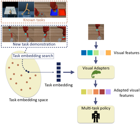
Figure 1: Task-conditioned adaptation: We show that a single policy can be trained to address multiple heterogenous tasks including manipulation, legged motion etc., and that few-shot learning is possible to address tasks given as demonstration but unseen during training. A key element is the task-conditioned adaptation of visual features.

Figure 2: Considered tasks: We train the method on a set $T^{k}$ of known tasks and evaluate it either on the same set, with the task known (   setting), or in a   setting, where a new unseen task from a set $T^{u}$ is inferred from a few demonstrations.

1 Introduction

Vision is one of the most important modalities for agents interacting with the world and is almost indispensable for dexterous manipulation or locomotion, as no other sensor can provide information as rich and versatile. The inherent flexibility of the sensor comes with a high price, the high dimensionality of the information, and the complexity of the processes necessary to extract useful information. Humans and other biological agents are capable of adapting their perception systems to the task at hand. There is indeed evidence for bottom-up and top-down processes in human vision, with the latter guiding attention to regions determined by the requirements of the task [6, 3].

There is a growing need for a similar versatility in artificial systems, and general neural networks have been trained from large-scale data in different domains such as natural language processing (NLP), computer vision (CV), and, more recently, robotics. A single general vision model coupled with a neural policy would be an appealing choice if it could allow an easy generalization to new domains or tasks. The wide adoption of attention mechanisms in several domains has made it easier for trained models to adapt their behavior to the requirements of different tasks without changing parameters, and it has been shown that attention plays a crucial role in specialization on a specific instance in language models [34] and vision and language models [15]. However, even powerful generally pre-trained models can benefit from parameter adaptations to specific tasks, either through fine-tuning [12] or by adding additional trained adapter layers to a frozen model [4].

In robotics, prior work on the generalization capabilities of agents has focused on large-scale end-to-end training [29] or, targeting vision specifically, on pre-trained visual models required to generalize to various different policies [20, 19, 21]. In this work, we argue and will show that a single policy can be trained for a large number of different tasks including manipulation, locomotion, and that the adaptation of visual features is highly beneficial, beyond the inherent adaptation capabilities of attention-based models. In particular, different tasks require diverse types of invariances and symmetries. While in principle it should be possible to learn to disentangle a sufficiently wide set of factors of variation in a captured representation such that it optimally performs on a wide variety of tasks, we will show that this is not the case for the arguably dominant pre-training method, masked auto-encoding (MAE) [9].

We propose task-conditioned adaptation, which allows leveraging the high-quality representations of generally pre-trained large vision models, while keeping the required flexibility to address a wide variety of tasks, and also new (unseen) tasks. We introduce a set of task-conditioned visual adapters that can be inserted inside a pre-trained visual Transformer [33]-based backbone. The task is characterized by an embedding space, which is learned from supervision during training. We show that this embedding space captures regularities of tasks and demonstrate this with few-shot capabilities: the single policy and (adapted) visual representations can address new unseen tasks, whose embedding is estimated from a few demonstrations (cf. Fig. 1).

The contributions of this work can be summarized as follows: (i) task-conditioned visual adapters to flexibly modulate visual features to a specific task; (ii) a single multi-task policy solving tasks with different embodiments and environments; (iii) a task embedding optimization procedure based on a few demonstrations of a new task (unseen at training time) to adapt the model in a few-shot manner without any weight fine-tuning; (iv) quantitative and qualitative results assessing the gain brought by the different novelties.

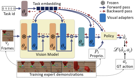
(a) Training the policy and adapters.
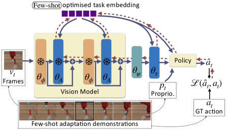
(b) Optimization of the task embedding for the   setting
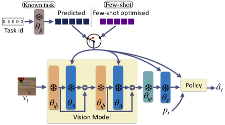
(c) Inference for the settings:   and .

Figure 3: Method overview: (a) the adapted policy is trained with behavior cloning from expert demonstrations and given a visual encoder pre-trained with masked auto-encoding. The model is conditioned on a task-embedding learned from GT 1-in-K task identifiers. (b) In the   case, a task embedding is estimated by optimization, maximizing the likelihood of a given demonstration of an unknown task. (c) Inference uses a task embedding given in the   case, or estimated in the   case.

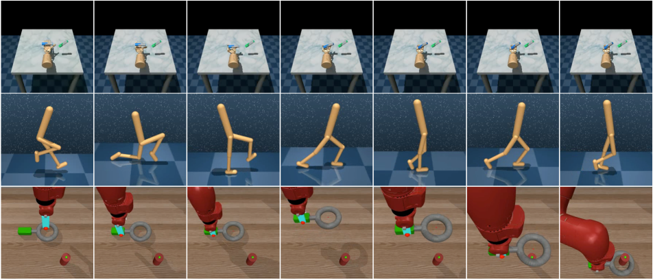
Figure 4:   — Qualitative results: Three successful policy rollouts on known tasks from the test set. The multi-task approach performs well on a variety of diverse tasks while being trained on a limited set of demonstrations.

2 Related Work

Pre-trained visual representations for robotics — Backbone models pre-trained on large and diverse data have shown great promises in NLP [14, 2, 24, 18], CV [26, 22, 9, 5], and more recently, robotics [20, 23, 21, 27, 19, 16, 35, 36]. Parisi et al. [23] study visual pre-training methods for visuo-motor control, showing the quality of self-supervised representations. Nair et al. [21] introduce R3M, a general vision model pre-trained on egocentric video data to capture temporal dynamics and semantic features, improving downstream manipulation performance. Radosavovic et al. [27] employ the well-known MAE framework [9] to pre-train a single vision encoder applied to robots in the real world. Ma et al. [19] pre-train a visual model with a self-supervised value function objective on egocentric human videos to improve the training of control policies. Finally, recent work [16, 35, 36] has shown the great promise of pre-trained models, either CLIP-based [16] or self-supervised [35, 36], in visual navigation.

The most related work is [20] which studies the impact of pre-trained vision models on a diversity of tasks gathered in a benchmark named Cortexbench. They introduce a Vision Transformer (ViT) [7] backbone, VC-1, pre-trained from a set of out-of-domain datasets with a focus on egocentric visual frames. We believe that visual features should be task-dependent and study how the VC-1 model can be adapted to improve the performance of a single multi-task policy on a subset of Cortexbench tasks, which is also different from previous work focusing on single-task policies.

Transformer adapters — Transferring Transformer [33]-based pre-trained models to new tasks or domains is an important topic. Methods involving adapter modules were introduced in NLP [10, 25, 11] to allow a fast and parameter-efficient transfer. Recent works employ the same methods in robotics [31, 17]. Sharma et al. [31] insert visual adapters in a Vision Transformer (ViT) [7] pre-trained model. They introduce different types of adapter blocks (”bottom”, ”middle”, ”top”) located at diverse places in the visual model and show that combining them improves performance. Liang et al. [17] also show the positive impact of inserting task-specific adapters, trained with imitation learning, in a pre-trained Transformer-based model to adapt to robotics tasks.

While prior work learns a specific set of adapters for each task, we argue that tasks share similarities and explore these regularities through a single multi-task policy.

Multi-task robotics policies — Having a single policy performing a wide range of tasks is a long-standing problem in robotics. With Deep Learning-based solutions becoming more popular, some prior work focuses on training multi-task neural agents. Approaches like BC-Z [13], RT-1 [1], RT-2 [38] or Gato [30] study the scaling abilities of neural models to large-scale datasets. Trained generalist agents show strong performance on a wide set of tasks, and can generalize to some extent to novel tasks.

In contrast, our work leverages pre-trained vision models but does not assume access to a large set of robotics data. Instead, we focus on how to adapt visual features with reasonable computation requirements and train a single multi-task policy from only a few expert demonstrations. We also show promising few-shot adaptation to new unknown tasks without requiring very diverse training data. Somewhat related to our work is also TD-MPC2 [8], which introduces a model-based RL algorithm to learn general world models and studies task embeddings to condition a multi-task policy. However, the latter does not act from vision while we specifically study how to modulate visual features conditioned by a task embedding.

3 Task-conditioned adaptation

All tasks considered in this work are sequential decision-making problems, where at each discrete timestep $t$ an agent receives the last $3$ visual frames as an observation $\mathbf{v}_{t}\in\mathbb{R}^{3\times h\times w\times 3}$, where $h$ and $w$ are the height and width of images, and a proprioception input $\mathbf{p}_{t}\in\mathbb{R}^{d_{a}}$, and predicts a continuous action $\mathbf{\hat{a}}_{t}\in\mathbb{R}^{d_{a}}$, where $d_{a}$ is the dimension of the action space, which depends on the task at hand. We are provided with a training dataset of expert demonstrations to train a single policy, and for inference we study two different setups: , where we a priori know the task to be executed, and , where the trained policy must be adapted to a new unseen task without fine-tuning only given a small set of demonstrations.

Known tasks — Following [20], we consider $K{=}12$ robotics tasks from $3$ benchmarks, Adroit [28], Deepmind control suite [32] and MetaWorld [37]. The set of all known tasks is denoted as $T^{k}=\{t_{i}^{k}\}_{[i=1..K]}$, where $t_{i}^{k}$ is a 1-in-K vector encoding a known task, and is illustrated in Figure 2.

Unknown tasks — The ability of our method to adapt to new skills is evaluated on a set of $U{=}15$ tasks from MetaWorld [37], for which we artificially generate demonstrations with a process described in section 4. The set of all unknown tasks is denoted as $T^{u}=\{t_{i}^{u}\}_{[i=1..U]}$, where $t_{i}^{u}$ is a 1-in-U vector encoding an unknown task, and is illustrated in Figure 2. Most importantly, $T^{k}\cap T^{u}=\emptyset$.

3.1 Base agent architecture

Following a large body of work in end-to-end training for robotics, the agent directly maps pixels to actions and decomposes into a visual encoder and a policy.

Visual encoder without adapters — following [20], the visual encoder, denoted as $\phi$, is a ViT model [7], which has been pre-trained with masked auto-encoding (MAE). We keep pre-trained weights from VC-1 in [20], which are publicly available. However, we change the way the representation is collected from the pre-trained model. Unlike [20], the representation is not taken as the embedding of the ’CLS’ token, which we consider to be undertrained by the MAE pretext task. Instead, we train a fully-connected layer $\psi$ to aggregate all the token representations of the last layer of the ViT except the ’CLS’ token. The visual observation $\mathbf{v}_{t}$ associated with timestep $t$ is thus encoded as

$$\mathbf{r}_{t}=\psi\bigr{[}\phi(\mathbf{v}_{t};{\theta}_{\phi});{\theta}_{\psi}\bigr{]},$$ (1)

where ${\theta}_{\phi}$ and ${\theta}_{\psi}$ are weights parametrizing $\phi$ and $\psi$, respectively. $\mathbf{r}_{t}\in\mathbb{R}^{3\times d_{r}}$ as it contains the $d_{r}$-dim encoding of each of the $3$ last visual frames processed as a data batch, where $d_{r}$ is the output dimension of $\psi$.

As this will become relevant later, we recall here that a ViT $\phi$ is composed of a sequence of $N_{s}$ self-attention blocks, where $\phi_{i}$ is the layer at index $i$. If we denote $\mathbf{s}^{i}_{t}$ as the internal hidden representation predicted at layer $i$, we have,

$$\mathbf{s}^{i}_{t}=\phi_{i}(\mathbf{s}^{i-1}_{t}))$$ (2)

where $\mathbf{s}^{0}_{t}{=}\mathbf{v}_{t}$.

Table 1:   — Impact of visual adapters: Validation and test performance on known tasks of different baselines highlighting the gain brought by adapters. Both visual and top adapters bring a boost in performance, and conditioning them on the learned task embedding increases performance. Our proposed architecture involving a multi-task policy outperforms single-task policies with VC-1 non-adapted features. MT $\pi$: multi-task policy – NC: Non-conditioned – C: Conditioned – Task emb.: whether to input at evaluation time, either the learned task embedding and chosen from ground-truth (L), a random vector as the task embedding (Rd), or a randomly picked task embedding among the set of $K{=}12$ embeddings (RdP) – Benchmarks avg: average performance accross the $3$ considered benchmarks (Adroit, DMC, MetaWorld) – Tasks avg: average performance across all $12$ known tasks.

	MT	Adapters		Task	Multi-task performance
	$\pi$	Mid.	Top	emb.	Adroit		DMC		MetaWorld		Benchmarks avg		Tasks avg
					Val	Test	Val	Test	Val	Test	Val	Test	Val	Test
(a) [20]	$-$	$-$	$-$	N/A	$44.0$ $\pm$ 1.1	$38.3$ $\pm$ 2.5	$49.6$ $\pm$ 0.5	$48.0$ $\pm$ 0.3	$53.5$ $\pm$ 2.1	$47.8$ $\pm$ 2.0	$49.1$ $\pm$ 0.5	$44.7$ $\pm$ 0.3	$50.3$ $\pm$ 0.9	$46.3$ $\pm$ 0.4
(b)	$\checkmark$	$-$	$-$	L	$36.3$ $\pm$ 1.7	$33.0$ $\pm$ 4.0	$55.3$ $\pm$ 1.4	$54.1$ $\pm$ 0.3	$41.7$ $\pm$ 1.6	$34.7$ $\pm$ 0.9	$44.4$ $\pm$ 1.0	$40.6$ $\pm$ 1.8	$46.5$ $\pm$ 1.1	$42.5$ $\pm$ 1.2
(c)	$\checkmark$	NC	$-$	L	$40.2$ $\pm$ 1.2	$37.3$ $\pm$ 2.8	$54.0$ $\pm$ 1.5	$54.8$ $\pm$ 1.9	$45.8$ $\pm$ 4.5	$36.3$ $\pm$ 2.5	$46.7$ $\pm$ 1.6	$42.8$ $\pm$ 1.9	$48.3$ $\pm$ 1.9	$44.2$ $\pm$ 1.8
(d)	$\checkmark$	C	$-$	L	$42.0$ $\pm$ 2.5	43.8 $\pm$ 2.2	$59.1$ $\pm$ 1.3	$58.8$ $\pm$ 0.3	$48.6$ $\pm$ 4.8	$40.8$ $\pm$ 3.0	$49.9$ $\pm$ 2.1	$47.8$ $\pm$ 1.4	$51.9$ $\pm$ 2.1	$48.8$ $\pm$ 1.3
(e)	$\checkmark$	C	NC	L	44.3 $\pm$ 1.2	$43.2$ $\pm$ 1.5	60.5 $\pm$ 0.5	60.3 $\pm$ 2.5	$58.6$ $\pm$ 1.6	$48.4$ $\pm$ 1.9	$54.5$ $\pm$ 0.7	$50.6$ $\pm$ 0.8	$57.0$ $\pm$ 0.7	$52.5$ $\pm$ 1.1
(f)	$\checkmark$	C	C	L	$42.0$ $\pm$ 0.8	$42.3$ $\pm$ 1.0	$59.9$ $\pm$ 0.9	$60.0$ $\pm$ 0.5	65.3 $\pm$ 1.0	54.5 $\pm$ 3.3	55.8 $\pm$ 0.1	52.3 $\pm$ 1.0	59.2 $\pm$ 0.1	54.8 $\pm$ 1.2
(g)	$\checkmark$	C	C	Rd	$4.2$ $\pm$ 4.0	$1.3$ $\pm$ 0.9	$10.3$ $\pm$ 0.7	$8.5$ $\pm$ 1.1	$1.3$ $\pm$ 0.9	$0.1$ $\pm$ 0.1	$5.3$ $\pm$ 0.8	$3.3$ $\pm$ 0.2	$5.5$ $\pm$ 0.1	$3.8$ $\pm$ 0.4
(h)	$\checkmark$	C	C	RdP	$0.7$ $\pm$ 0.9	$3.2$ $\pm$ 2.5	$5.7$ $\pm$ 1.2	$9.5$ $\pm$ 6.1	$0.9$ $\pm$ 0.6	$0.3$ $\pm$ 0.4	$2.4$ $\pm$ 0.5	$4.3$ $\pm$ 2.2	$2.9$ $\pm$ 0.4	$4.6$ $\pm$ 2.5

Single-task policy — again following [20], the policy $\pi$ is memory-less and implemented as an MLP predicting actions from the input which is a concatenation of the current frame, two frame differences and the proprioception input $\mathbf{p_{t}}$,

$$\hat{\mathbf{a}}_{t}=\pi\left(\Bigr{[}\mathbf{r}_{t,1}{-}\mathbf{r}_{t,0},\mathbf{r}_{t,2}{-}\mathbf{r}_{t,1},\mathbf{r}_{t,2},\mathbf{p_{t}}\Bigr{]};{\theta}_{\pi}\right),$$ (3)

where $[~{}]$ is the concatenation operator and ${\theta}_{\pi}$ are weights parametrizing $\pi$.

3.2 Adaptation

Our key contributions are visual adapter modules along with a multi-task policy, which are all conditioned on the task at hand. This is done with a specific task embedding for each task, taken from an embedding space of dimension $d_{e}$, which is aimed to have sufficient regularities to enable few-show generalization to unseen tasks. Importantly, the different adapters and the multi-task policy are conditioned on the same task embedding, leading to a common and shared embedding space. For the known task setting, where the ground-truth label of the task is available, the task embedding is projected from a 1-in-K vector with a linear function $g$ trained jointly with the adapters and the policy with the downstream loss (imitation learning). In the Few-shot setting, at test time a new unknown task is described with a few demonstrations, and a task embedding is estimated through optimization, as will be detailed in subsection 3.4. Figure 3 outlines the architecture, its details will be given in the supplementary material.

Conditioned on a task embedding we denote as $\mathbf{e}$, the proposed adaptations are based on “middle” and “top” adapters following [10, 31].

Middle adapters — we add one trainable adapter after each such ViT block to modulate its output. We introduce a set of middle adapters $A=\{\alpha_{i}\}_{[i=1..N_{s}]}$, where $\alpha_{i}$ is a 2-layer MLP. In the modified visual encoder $\phi^{m}$, each adapter modulates the output of the corresponding self-attention block and is conditioned on the task embedding $\mathbf{e}$. The output of a middle adapter is combined with the one of the self-attention layer through a residual connection. If we denote $\mathbf{s}^{m,i}_{t}$ as the internal hidden representation predicted at layer $i$, the associated forward pass of a given layer becomes,

$$\mathbf{s}^{m,i}_{t} =\phi^{m}_{i}(\mathbf{s}^{m,(i-1)}_{t})$$ (4)

$$=\phi_{i}(\mathbf{s}^{m,(i-1)}_{t})+\alpha_{i}(\phi_{i}(\mathbf{s}^{m,(i-1)}_{t}),\mathbf{e})$$ (5)

$$=\mathbf{s}^{i}_{t}+\alpha_{i}(\mathbf{s}^{i}_{t},\mathbf{e})$$ (6)

Top adapter — A top adapter $\tau$, also conditioned on the task at hand, is added after the ViT model, to transform the output of the aggregation layer $\psi$ to be fed to the multi-task policy (presented below). $\tau$ has the same architecture as a single middle adapter $\alpha_{i}$. The prediction of $\mathbf{r}_{t}^{m}$, equivalent to $\mathbf{r}_{t}$ in the non-adapted case, can be written as,

$$\mathbf{r}_{t}^{m}=\tau\Bigr{[}\psi\bigr{[}\phi^{m}(\mathbf{v}_{t},\mathbf{e};{\theta}_{\phi},{\theta}_{A});{\theta}_{\psi}\bigr{]},\mathbf{e};\theta_{\tau}\Bigr{]}$$ (7)

where ${\theta}_{A}$ and ${\theta}_{\tau}$ are the weights parametrizing the middle adapters (each middle adapter has a different set of weights) and the top adapter respectively.

Multi-task policy — We keep the architecture of the single-task policy in eq. (3), as in  [20]. However, instead of re-training a policy for each downstream task of interest, we train a single multi-task policy $\pi^{m}$, whose action space is the union of the action spaces of the different tasks. During training we apply a masking procedure on the output, considering only the actions possible for the task at hand.

Let’s denote $\mathbf{\tilde{r}}^{m}_{t}$ as the input to the policy derived from the adapted representation $\mathbf{r}^{m}_{t}$ and the proprioception input $\mathbf{p_{t}}$ as done in eq. (3). The conditioning on the task is done by concatenating $\mathbf{\tilde{r}}^{m}_{t}$ with the task embedding $\mathbf{e}$, giving

$$\hat{\mathbf{a}}_{t}=\pi^{m}\left(\left[\mathbf{\tilde{r}}^{m}_{t},\mathbf{e}\right],{\theta}_{\pi^{m}}\right),$$ (8)

where ${\theta}_{\pi^{m}}$ are weights parametrizing $\pi^{m}$.

Figure 5:   — Per-task performance: performance of single-task policies (row (a) in Table 1), our approach without any adapter (row (b) in Table 1) and with conditioned middle and top adapters (row (f) in Table 1). The proposed adapters lead to a performance gain on most tasks, and our multi-task solution is competitive with single-task policies.

3.3 Training

We train the model by keeping the weights of the pre-trained vision-encoder model $\theta_{\phi}$ frozen, only the weights of the adapter modules (${\theta}_{A}$, ${\theta}_{\tau}$), aggregation layer (${\theta}_{\psi}$), embedding layer ($\theta_{g}$) and multi-task policy (${\theta}_{\pi^{m}}$) are trained, cf. Fig. 3a. Lets’ denote by $\Theta{=}{\{\theta}_{A},{\theta}_{\tau},{\theta}_{\psi},{\theta}_{g},{\theta}_{\pi^{m}}\}$ the set of optimized weights. We train with imitation learning, more specifically Behavior Cloning (BC): for each known task $t_{i}^{k}$, we have access to a set of $N_{i}$ expert trajectories that are composed of $T_{i}$ discrete steps, including expert actions. The optimization problem is given as

$$\hat{\Theta}=\arg\min_{\Theta}\sum_{i=1}^{K}\sum_{n=1}^{N_{i}}\sum_{t=1}^{T_{i}}\mathcal{L}(\hat{\mathbf{a}}_{t},{\mathbf{a}}_{t}^{i,n})$$ (9)

where ${\mathbf{a}}_{t}^{i,n}$ is the ground-truth expert action for a given step in a trajectory, and $\mathcal{L}$ is the Mean Squared Error loss.

3.4 Few-shot adaption to new tasks

For the   setting, the task embedding $\mathbf{e}$ is unknown at inference and needs to be estimated from a set of $N_{d}$ example demonstrations $\mathcal{D}=\{d_{i}\}_{i=1..N_{d}}$ where $d_{i}=\{(\mathbf{v}^{i*}_{t},\mathbf{p}^{i*}_{t},\mathbf{a}^{i*}_{t})\}_{t=1..T}$ is composed of observations and actions. We exploit the conditioning property of the policy itself to estimate the embedding $\hat{\mathbf{e}}$ as the one which obtains the highest probability of the demonstration actions, when the policy is applied to the demonstration inputs, i.e.

$$\hat{\mathbf{e}}=\arg\min_{\mathbf{e}}\sum_{i}\sum_{t}\mathcal{L}(\pi^{m}\left(\left[\mathbf{\tilde{r}}^{mi*}_{t},\mathbf{e}\right],\theta_{\pi^{m}},\right),{\mathbf{a}}_{t}^{i*}),$$ (10)

where $\mathbf{\tilde{r}}^{mi*}$ is the representation extracted from the demonstration input $(\mathbf{v}^{i*}_{t},\mathbf{p}^{i*}_{t})$, and which itself depends on $\mathbf{e}$ (this is not made explicit in the notation). The minimization is carried out with SGD from an embedding initialized to zero.

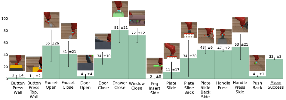
Figure 6:   — Per-task performance on unknown tasks: After optimizing the task embedding independently for each task from 5 demonstrations, our method can adapt to many of them, without requiring any weight finetuning.

4 Experiments

Training — all variants involving adapters and/or a multi-task policy (rows (b)-(f) in Table 1) were trained for $50$ epochs with behavior cloning, cf. §3.3, following training hyper-parameters in [20]. Between $20$ and $95$ expert trajectories are available depending on the task. We used the datasets of trajectories from [20].

Evaluation — to better handle possible overfit on hyper-parameter selection, our evaluation setup is slightly different from [20] as we perform $100$ validation rollouts to select the best checkpoint of each model, and then test the chosen model on $100$ test rollouts. For our multi-task policy, the best checkpoint is the one with the highest average validation performance across all tasks. Single-task policies are validated only on the task they were trained on, giving them an advantage, and for this reason, they are reported as “soft upper bounds”. We report the average performance and standard deviation among $3$ trained models (3 random seeds) for each variant.

In total, we conduct evaluations of our method on $27$ different tasks, $12$ known and $15$ unknown, with varying environments, embodiments, and required sub-skills. This allows to evaluate the adaptation and generalization abilities of the multi-task policy.

Evaluation metrics — Following [20], we consider a rollout success ($1$ if the task was completed properly, $0$ otherwise) for tasks in the Adroit and MetaWorld benchmarks, and report the agent’s normalized return for Deepmind Control. Performance is averaged across rollouts. Episodes have a maximum length of $1000$ steps and each step reward is comprised between $0$ and $100$ in DMC, normalization is therefore done by dividing the agent’s return by $10$.

— Impact of visual adapters — Table 1 presents a detailed comparison of different methods on the known task setting. The baseline in row (a) follows the setup in [20] to train single-task policies (one for each task) from non-conditioned VC-1 features. For this variant, we also use the representation of the ’CLS’ token as the vector fed to the policy as done to respect its original choice, while all other baselines use our proposed token aggregation layer.

Row (b) is our multi-task policy without any adapter, as expected there is some performance drop when compared to the specialized policies in row (a), as the problem to solve has become more difficult. Adding adapters and conditioning them on the task embedding, shown in rows (c)-(f), brings a boost in performance, both for middle and for top adapters. In particular, conditioning adds a further boost compared to non-conditioned adapters, with all choices enabled, row (f), obtaining the best average performance.

Rows (g) and (h) are ablation experiments that evaluate the impact of choosing completely random task embeddings, row (g), or of taking a random choice between the 12 learned embeddings, row (h). In both cases, the performance collapses.

A particularly important conclusion that can be drawn from the experiments outlined in Table 1 is that the proposed multi-task approach (row (f)) outperforms the single-task policies without adapters (row (a)). This shows that a multi-task policy can perform well on a series of tasks while being trained on a limited set of demonstrations. Figure 4 presents $3$ successful test rollouts of our multi-task approach on diverse known tasks.

Figure 5 visualizes the per-task test performance on known tasks of single-task policies (row (a) in Table 1), our approach without any adapter (row (b) in Table 1) and with conditioned middle and top adapters (row (f) in Table 1). The proposed adapters lead to a performance gain on most tasks compared with the solution without adapters, and the multi-task solution is competitive with single-task policies, even outperforming them on half the tasks.

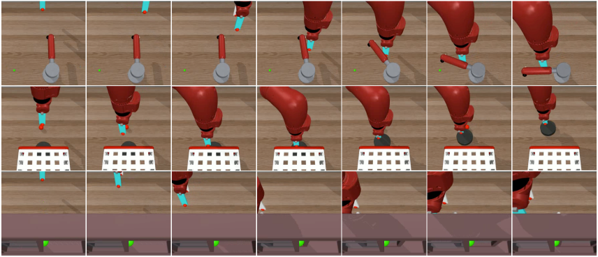
Figure 7:   — Qualitative results on unknown tasks: Three successful policy rollouts on unknown tasks. The multi-task approach tackles these new tasks involving different objects or manipulation requirements than what it was trained on.

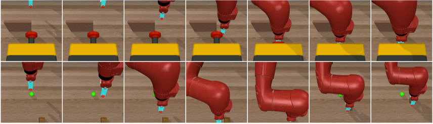
Figure 8:   — Failure cases on unknown tasks: The first row (button-press-wall task) shows an example where the method performs the task correctly until the end where it fails to properly push the button fully. This behavior seems to happen often for this button-press-wall task, explaining its $0\%$ success despite being able to reproduce most of the behavior. In the second row (push-back task), the policy is able to properly move the cube but fails to bring it to the goal position (green dot).

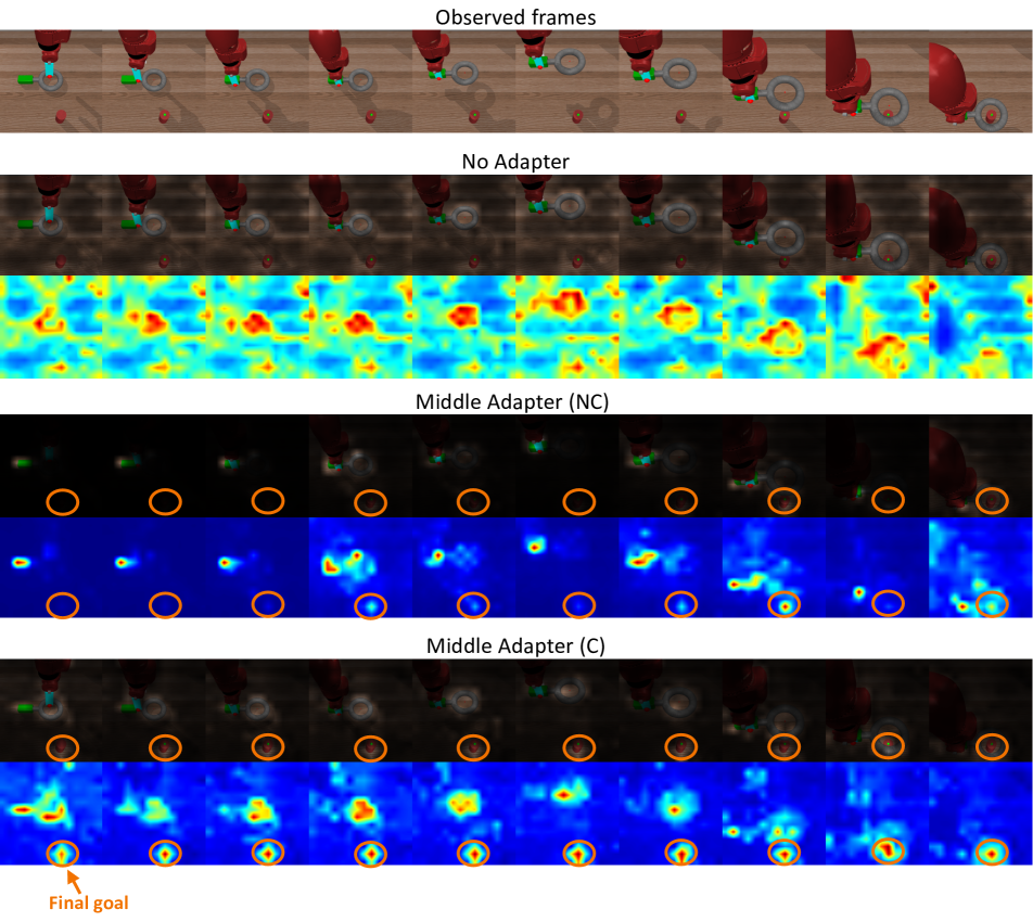
Figure 9: Visualization of attention maps (Assembly task). First row: observed input frames. Following blocks: for each model type, we show the attention map of the last ViT layer, first overlaid on top of the visual frame and below as a colored heatmap. In this example, middle adapters allow to focus the attention on important regions, and task conditioning leads to a better covering of entire objects and agent parts, along with greater attention towards the final goal for all frames.

— Additional ablation studies — are presented in the appendix (Sections B, C). Section B shows that conditioning the policy when using task-conditioned adapters is not necessary, that our aggregation layer works better than using the ’CLS’ token as input to the policy and further highlights the impact of both middle and top adapters. Section C shows that our adapters improve visual embeddings extracted by two other state-of-the-art pre-trained backbones, i.e. PVR [23] and MVP [27], confirming the conclusions drawn from experiments on VC-1.

— adaptation to new tasks without finetuning model weights is an important ability of any general policy, which we evaluate with the following experiments: for each task within a set of unknown tasks (cf. Figure 2), we collect only $5$ demonstrations used to optimize a task embedding specific to this task with the method detailed in section §3.4. We then test the method conditioned on the optimized embedding on $100$ test rollouts.

To generate the set $T^{u}$ of unknown tasks, we select tasks from the MetaWorld dataset which had not been selected for the CortexBench benchmark, and which are therefore not part of the set of known tasks $T^{k}$ on which we trained the policy and adapters. Unfortunately for these tasks, there do not exist expert demonstrations as they have been defined as environments for RL training only. We collect demonstrations using single-task policies from TD-MPC2 [8] that were specifically trained on each task of MetaWorld independently. To ensure high-quality demonstrations, we only consider tasks where TD-MPC2 policies reach a success rate higher than $95\%$. Furthermore, to be compatible with the choices of the CortexBench authors, in particular, to keep the same camera locations, we filter out some of the tasks where the goal is not always visible in the camera FOV. This leads to a set of $15$ unknown tasks that are quite different from the tasks in the training set $T^{k}$ as they involve different objects (handle press, faucet, plate, door, window, etc.) and types of manipulation (sliding an object, lowering a press, opening a window, etc.). Each collected demonstration is a sequence of visual frames, proprioception inputs, and expert actions. The optimization of the task embedding is performed independently for each task (cf. §3.4). We use the AdamW optimizer and a learning rate of $1e{-1}$ during the task embedding search.

Figure 6 presents the per-task performance in this setting. Despite the large variations in terms of objects and types of manipulations between the new tasks in $T^{u}$ and the ones in the training set ($T^{k}$), the proposed multi-task policy can adapt to many of them, without requiring any weight finetuning. Interestingly, the method performs particularly well on the Drawer Close task, as the time-inversed Drawer Open task was in the training set. This provides some evidence that the method can exploit regularities between tasks, which seem to be captured by the task embedding space, making it possible to generalize to unseen variations. Figure 7 shows qualitative examples of successful rollouts on the new tasks. The multi-task policy is able to manipulate new objects (faucet, plate, window) that were not encountered at training time. It also successfully performs diverse new moves such as rotating the faucet or sliding the plate.

Finally, Figure 8 shows failure cases of our method on unknown tasks. As can be seen on the first row, the policy avoids the wall, reaches the button, and starts pushing it, but fails to push it fully. This particular behavior was also observed on other rollouts, explaining the $0\%$ success on this button-push-wall task while mastering a part of the required sub-skills. On the second row, the policy is being evaluated on the push-back task. It is able to move the cube but fails to bring it to the goal location (green dot). This gives some indication of the difficulty of the few-shot generalization case: exploiting regularities in the task space requires that tasks be performed more than just approximately, as often the success metric is sparse, and rollouts only count to the metric when they are executed fully and correctly.

Visualizing the influence of task-conditioned adaptation — Sequences of visual frames used in this experiment are taken from a held-out set of expert trajectories not used at training time. We visualize here the attention map of the last layer of the vision encoder. To this end, we sum attention maps for all tokens and all heads, and normalize them between $0$ and $1$. These visualizations are shown in Figures 9. The first row shows a sequence of visual frames and below, for each model variant (No Adapter, Middle Adapter (NC), Middle Adapter (C)), one can see the attention map overlaid on top of the visual frame and displayed below as a colored heatmap. As can be seen, the middle adapters help focus the attention on the most important parts of the image compared with vanilla VC-1 attention without adapters. When adapters are not conditioned (NC), they tend to produce very narrow attention. Conditioning on the task at hand keeps the focus on important regions and leads to covering the entire objects of interest and important agent parts. Most importantly, Figure 9 shows that, when adapters are conditioned on the task embedding, more attention is put on the final goal in all frames, while this is not the case for unconditioned adapters. Another visualization is shown in Figure 11 in the appendix.

5 Conclusion

Perception and action are closely tied together, and studies of human cognition have shown that a priori knowledge about a downstream task guides the visual system. We follow this direction in the context of artificial agents by introducing task-conditioned adapters that modulate the visual features of a pre-trained neural backbone. Such adapters, conditioned on a learned task embedding, improve the performance of a multi-task policy across benchmarks and embodiments. Even more interesting is the use of task embeddings to adapt in a few-shot manner, i.e. from a small set of demonstrations, to new tasks unseen at training time. We propose an optimization procedure to estimate a new task embedding and achieve generalization to unseen tasks, involving new objects and manipulation sub-skills, providing evidence for regularities in the learned embedding space.

Appendix

Appendix A Validation performance curves

Figure 10 shows the evolution of the validation score as a function of training epochs for rows (b)-(f) in Table 1 of the main paper. These curves showcase the gain brought by both middle and top adapters, and the positive impact of conditioning them on the task at hand.

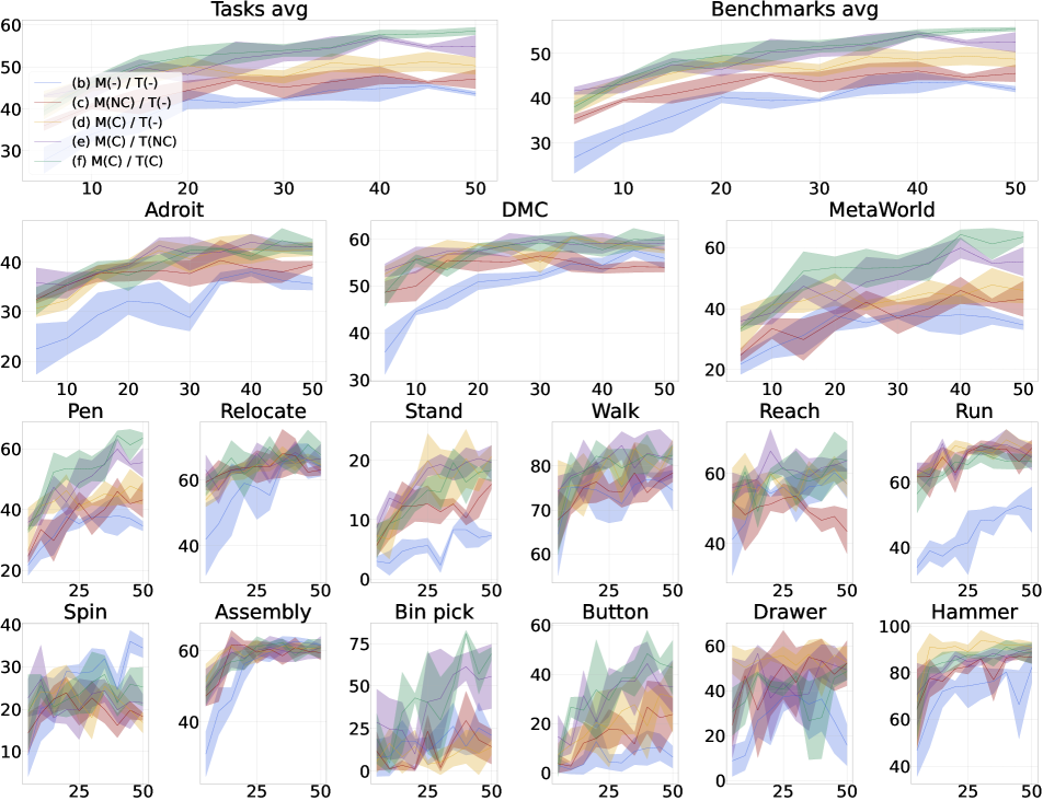
Figure 10:   — Impact of visual adapters: Evolution of the validation performance during training for rows (b)-(f) in Table 1 of the main paper. In the legend, M and T refer respectively to the state of middle and top adapters, and -, NC or C mean they are absent, not conditioned or conditioned on the task embedding. On all plots, the y-axis represents the performance score and the x-axis corresponds to the training epoch. Colored lines represent the evolution of mean performance over 3 training runs (3 random seeds) and shaded areas represent standard deviation.

Appendix B Additional ablation studies

Impact of conditioning the policy on the task at hand — Row (b) in Table 2 reaches the same performance, even slightly better, as row (a), showing that when adapters are conditioned on the task at hand, conditioning the policy itself is not necessary. This seems to indicate that conditioned adapters already insert task-related information into visual embeddings fed to the policy.

Using the ’CLS’ token representation as input to the policy — Row (c) in Table 2 performs worse than row (a), indicating that our introduced tokens aggregation layer $\psi$ improves over the strategy used in previous work consisting in feeding the output ’CLS’ token to the policy. This confirms our assumption that the ’CLS’ token is undertrained under the MAE pre-training task.

Impact of the middle adapters when using top adapters — Row (d) in Table 2 also performs worse compared with row (a), showing that when training a conditioned top adapter, middle adapters are still very important, bringing a significant boost in performance.

Table 2:   — Additional ablation studies: Validation and test performance on known tasks of different neural variants. Row (a) is equivalent to row (f) in Table 1 of the main paper. When using conditioned adapters, giving the task embedding as input to the policy is not necessary. Our introduced tokens aggregation layer is better than using the representation of the ’CLS’ token. Finally, when training a conditioned top adapter, middle adapters are still important and bring a boost in performance. Cond $\pi$: policy conditioned on the task embedding – C: Conditioned – ’CLS’ token: using the ’CLS’ token representation as the frame embedding fed to the policy.

Cond.

Adapters

’CLS’

Multi-task performance

$\pi$

Mid.

Top

token

Adroit

DMC

MetaWorld

Benchmarks avg

Tasks avg

Val

Test

Val

Test

Val

Test

Val

Test

Val

Test

(a)

$\checkmark$

C

C

$-$

$42.0$ $\pm$ 0.8

$42.3$ $\pm$ 1.0

$59.9$ $\pm$ 0.9

$60.0$ $\pm$ 0.5

$65.3$ $\pm$ 1.0

$54.5$ $\pm$ 3.3

$55.8$ $\pm$ 0.1

$52.3$ $\pm$ 1.0

$59.2$ $\pm$ 0.1

$54.8$ $\pm$ 1.2

(b)

$-$

C

C

$-$

$42.3$ $\pm$ 2.0

$40.8$ $\pm$ 3.0

$59.2$ $\pm$ 1.0

$59.2$ $\pm$ 2.3

$68.7$ $\pm$ 2.2

$57.6$ $\pm$ 3.4

$56.8$ $\pm$ 0.8

$52.5$ $\pm$ 0.9

$60.4$ $\pm$ 0.8

$55.5$ $\pm$ 0.5

(c)

$\checkmark$

C

C

$\checkmark$

$38.8$ $\pm$ 5.9

$36.2$ $\pm$ 2.3

$57.8$ $\pm$ 1.9

$58.1$ $\pm$ 2.6

$57.5$ $\pm$ 8.0

$50.9$ $\pm$ 4.3

$51.4$ $\pm$ 2.8

$48.4$ $\pm$ 0.6

$54.5$ $\pm$ 2.9

$51.4$ $\pm$ 1.3

(d)

$\checkmark$

$-$

C

$-$

$34.7$ $\pm$ 1.5

$34.7$ $\pm$ 3.3

$51.4$ $\pm$ 0.4

$52.1$ $\pm$ 0.5

$53.6$ $\pm$ 4.4

$44.5$ $\pm$ 4.7

$46.6$ $\pm$ 1.6

$43.8$ $\pm$ 1.8

$49.5$ $\pm$ 2.0

$46.0$ $\pm$ 1.9

Table 3:   — Impact on other visual backbones: Validation and test performance on known tasks for two additional visual backbones (PVR [23] and MVP [27]). Our task-conditioned adapters improve the extracted visual features in both cases, leading to higher multi-task policy performance.

ViT	Ours	Multi-task performance
		Adroit		DMC		MetaWorld		Benchmarks avg		Tasks avg
		Val	Test	Val	Test	Val	Test	Val	Test	Val	Test
PVR [23]	$-$	$34.5$${\pm}$2.8	$33.7$${\pm}$2.3	$57.1$${\pm}$2.0	$57.1$${\pm}$2.6	$37.8$${\pm}$5.8	$31.7$${\pm}$4.1	$43.1$${\pm}$1.4	$40.8$${\pm}$0.5	$45.3$${\pm}$1.6	$42.6$${\pm}$0.5
	$\checkmark$	42.5${\pm}$3.0	39.5${\pm}6.1$	$58.5$${\pm}$1.9	59.7${\pm}$2.4	68.7${\pm}$3.3	57.7${\pm}$5.5	56.6${\pm}$0.2	52.3${\pm}1.4$	60.1${\pm}$0.7	55.5${\pm}$1.1
MVP [27]	$-$	$38.0$${\pm}$1.3	$34.3$${\pm}$2.4	$56.5$${\pm}$2.1	$56.5$${\pm}$1.7	$42.8$${\pm}$6.9	$35.9$${\pm}$5.6	$45.8$${\pm}$1.5	$42.2$${\pm}$2.2	$47.7$${\pm}$1.9	$44.2$${\pm}$2.2
	$\checkmark$	47.7${\pm}$5.9	46.2${\pm}$2.4	$57.3$${\pm}$2.9	$56.9$${\pm}$2.5	64.9${\pm}$12.1	55.4${\pm}$12.2	56.6${\pm}$4.0	52.8${\pm}$2.6	58.9${\pm}$4.4	54.5${\pm}$3.8

Table 4: Non-linear probing of actions: we explore the performance of action regression from the visual embedding of a single frame. Considered metrics are the Mean Squared Error (MSE) and coefficient of determination ($R^{2}$). The top adapter seems to insert action-related information into the visual embedding, as the probing MLP achieves the best performance.

	Middle adapters	Top adapter	MSE	$R^{2}$
(a)	$-$	$-$	$0.067$	$0.69$
(b)	NC	$-$	$0.069$	$0.57$
(c)	C	$-$	$0.069$	$0.59$
(d)	C	NC	$0.037$	$0.90$
(e)	C	C	0.034	0.92

Table 5:   — Diversity of known tasks: Validation and test performance on MetaWorld known tasks when our approach with task-conditioned adapters is either trained on the three considered benchmarks (Adroit, DMC, MetaWorld), or on tasks from MetaWorld only. As expected, the model trained on known tasks from MetaWorld only reaches higher performance.

	Training	MetaWorld
		Val	Test
(a)	All 3 benchmarks	$65.3$$\pm$1.0	$54.5$ $\pm$3.3
(b)	MetaWorld only	$75.6$$\pm$1.6	$67.8$$\pm$2.6

Table 6:   — Performance of a finetuned baseline (Ft.) and task embedding search for a policy either trained on MetaWorld only or all 3 benchmarks. $t_{i}^{u}$ refers to the $i$-th unknown task.

	Opt.	Train.	Setting	$t_{0}^{u}$	$t_{1}^{u}$	$t_{2}^{u}$	$t_{3}^{u}$	$t_{4}^{u}$	$t_{5}^{u}$	$t_{6}^{u}$	$t_{7}^{u}$	$t_{8}^{u}$	$t_{9}^{u}$	$t_{10}^{u}$	$t_{11}^{u}$	$t_{12}^{u}$	$t_{13}^{u}$	$t_{14}^{u}$	Mean
(a)	TE opt.	All 3	Single policy	$2$${\pm}$4	$1$${\pm}$2	$55$ ${\pm}$26	$41$${\pm}$21	$4$${\pm}$4	$34$${\pm}$10	$81$${\pm}$21	$72$${\pm}$12	$0$${\pm}$0	$11$${\pm}$17	$34$${\pm}$30	$48$${\pm}$6	$47$${\pm}$2	$53$${\pm}$21	$4$${\pm}$1	$33$${\pm}$2
(b)	Ft.	All 3	$15$ policies	$1$${\pm}$2	$0$${\pm}$0	$49$${\pm}$44	$69$${\pm}$22	$5$${\pm}$2	$62$${\pm}$8	$96$${\pm}$4	$91$${\pm}$7	$2$${\pm}$3	$54$${\pm}$8	$50$${\pm}$4	$22$${\pm}$19	$66$${\pm}$7	$89$${\pm}$1	$3$${\pm}$2	$44$${\pm}$3
(c)	TE opt.	MW	Single policy	$3$${\pm}$6	$0$${\pm}$0	$56$${\pm}$44	$64$${\pm}$20	$1$${\pm}$2	$69$${\pm}$19	$100$${\pm}$0	$77$${\pm}$20	$0$${\pm}$1	$6$${\pm}$6	$22$${\pm}$38	$19$${\pm}$3	$55$${\pm}$13	$57$${\pm}$17	$5$${\pm}$3	$36$${\pm}$5

Appendix C Impact on other visual backbones

Table 3 shows the impact of our task-conditioned adapters on the visual features extracted by two other SOTA ViT-B backbones, i.e. PVR [23] and MVP [27]. As can be seen, our adapters bring a boost in policy performance for both pre-trained backbones, generalizing the conclusions obtained with VC-1.

Appendix D Visualizing the influence of task-conditioned adaptation

This section focuses on investigating the impact of the introduced adapters on the processing of visual features. All sequences of visual frames used in the following experiments are taken from a held-out set of expert trajectories not used at training time.

Influence of middle adapters on ViT attention maps — Figure 11 presents another visualization (see also Figure 9 in the main paper) of the attention map of the last layer of the vision encoder: we sum attention maps for all tokens and all heads, and normalize them between $0$ and $1$. The first row shows a sequence of visual frames and below, for each model variant (No Adapter, Middle Adapter (NC), Middle Adapter (C)), one can see the attention map overlaid on top of the visual frame and displayed below as a colored heatmap.

Figure 11 confirms that middle adapters lead to better-focused attention around important objects related to the task, compared with vanilla VC-1. Unconditioned adapters (NC) tend to either produce very narrow (first frames in Figure 11) or quite broad (last frames in Figure 11) attention. Task conditioning leads to a better coverage of entire objects and important agent parts. As already mentioned in the main paper, conditioning on the task at hand improves the attention towards the final goal to reach.

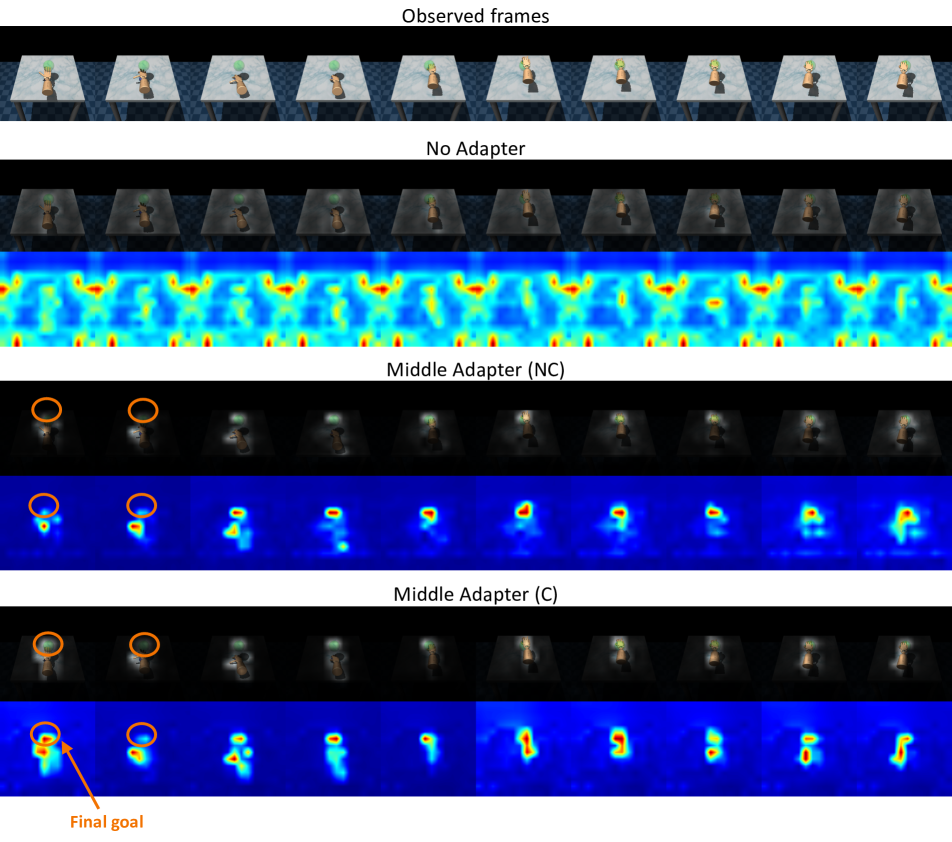
Figure 11: Visualization of attention maps (Relocate task). First row: observed input frames. Following blocks: for each model type, we show the attention map of the last ViT layer, first overlaid on top of the visual frame and below as a colored heatmap. In this example, middle adapters allow to focus the attention on important regions, and task conditioning leads to a better covering of the robotic hand and the sphere goal in all frames.

Conditioning middle adapters helps insert task-related information into visual embeddings — In order to study the underlying mechanisms of adapter modules, we examine the content of produced visual embeddings. Figure 13 shows t-SNE plots of visual embeddings for a set of frames for both the DMC Stand and Walk tasks. Visual observations are identical for both tasks at the beginning of rollouts, and very similar in the rest of the sequences, making it very hard to distinguish between these $2$ tasks from a visual observation only. Embeddings from the conditioned middle adapters form two well-separated clusters, showcasing the task-related information brought by conditioning adapters on the task at hand.

Figure 12: Task-related information inside visual embeddings: t-SNE plots of visual embeddings for a set of frames for DMC Stand and Walk tasks. We chose these tasks for their visual similarity, making it very hard to distinguish between them from vision only. Conditioning of the middle adapters leads to two properly separated clusters, showing the insertion of task-related information into the visual embedding.

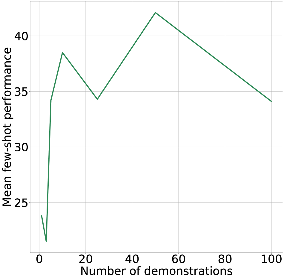
Figure 13:   — Impact of the number of demonstrations on few-shot adaptation to unseen tasks: Few-shot performance as a function of the number of demonstrations used to optimize the task embedding. We can achieve $23.8\%$ from a single demonstration, and more demonstrations can lead to higher performance. However, the trend is not as simple as $100$ demonstrations lead to the same performance as $5$ demonstrations.

Appendix E Non-linear probing of actions

Table 4 shows the performance of a probing MLP network trained to regress the expert action to take from the visual embedding of a single frame only. As can be seen, its performance improves drastically when trained on embeddings predicted by a vision encoder composed of conditioned middle and top adapters. A conditioned top adapter thus inserts action-related information within visual embeddings.

Appendix F Diversity of known tasks

Tab. 6 (c) and Tab. 5 (b) shows a model trained on MetaWorld only, which performs better on MetaWorld than models trained on all 3 benchmarks (the domain gap between them is large). The lower performance on MetaWorld when training on all 3 benchmarks is largely outweighed by the ability to address Adroit and DMC.

Appendix G Few-shot adaptation baseline

Table 6 compares model finetuning on new tasks (b) with our task embedding search (a). As expected, (b) performs better but task embedding search (a) solves a harder problem, as we keep a single policy. Our adapters can thus be used in $2$ settings: (i) task embedding search, keeping a single policy addressing all tasks (low memory footprint), (ii) task-specific fine-tuning to reach the best performance possible if memory is not an issue (one specific set of $130$M parameters for each task).

Appendix H Architecture details

Vision encoder — we use a ViT-B backbone, initialized from VC-1 weights, as the base vision encoder $\phi$. It is made of $12$ self-attention layers, each composed of $12$ attention heads, with a hidden size of $768$. The input image of size $224{\times}224{\times}3$ is divided into a grid of $14{\times}14$ patches, where each patch has thus a size of $16{\times}16$ pixels. An additional ’CLS’ token is appended to the sequence of image tokens to follow the setup used to pre-train the model.

Task embedding — the task embedding is a $1024$-dim vector. For known tasks, it is predicted by a linear embedding layer from a 1-in-K vector where $K{=}12$.

Middle adapters — one adaptation module $\alpha_{i}$ is inserted after each self-attention layer inside $\phi$. It is composed of $2$ fully-connected layers with respectively $384$ and $768$ neurons. A GELU activation function is applied to the output of the first layer. The input to a middle adapter is the concatenation of the task embedding and a token representation from the previous self-attention layer. It thus processes all tokens as a batch.

Aggregation fully-connected layer — the input to the aggregation fully-connected layer $\psi$ is a concatenation of the $768$-dim representation of all $14{\times}14{=}196$ tokens. It is implemented as a simple fully-connected layer predicting a $768$-dim vector representation.

Top adapter — the top adapter $\tau$ is fed with the output of $\psi$, again concatenated to the task embedding. It is composed of $2$ fully-connected layers that both have $768$ neurons. A ReLU activation function is applied to the output of the first layer.

Multi-task policy — The policy $\pi^{m}$ is a $3$-layer MLP, with $256$ neurons for all layers and $ReLU$ activation functions. A batch normalization operation is applied to the input to the policy. $\pi^{m}$ outputs a $30$-dim action vector, as $30$ is the number of components in the action space with the most components among the $12$ known tasks. When solving a task with a smaller action space, we mask out the additional dimensions.

Appendix I Impact of the number of demonstrations on few-shot adaptation to unseen tasks

Figure 13 presents the evolution of the average few-shot performance of our method across the $15$ unknown tasks depending on the number of available demonstrations when optimizing the task embedding. From only a single demonstration per task, we can already reach a satisfying $23.8\%$ mean performance. Adding more demonstrations can allow to reach higher performance, but the scaling law does not appear to be as simple as using $100$ demonstrations leads to the same final performance as $5$ demonstrations.

References

- Brohan et al. [2022] Anthony Brohan, Noah Brown, Justice Carbajal, Yevgen Chebotar, Joseph Dabis, Chelsea Finn, Keerthana Gopalakrishnan, Karol Hausman, Alex Herzog, Jasmine Hsu, et al. Rt-1: Robotics transformer for real-world control at scale. arXiv, 2022.
- Brown et al. [2020] Tom Brown, Benjamin Mann, Nick Ryder, Melanie Subbiah, Jared D Kaplan, Prafulla Dhariwal, Arvind Neelakantan, Pranav Shyam, Girish Sastry, Amanda Askell, et al. Language models are few-shot learners. NeurIPS, 2020.
- Buschman and Miller [2007] T. J. Buschman and E. K. Miller. Top-down versus bottomup control of attention in the prefrontal and posterior parietal cortices. science, 2007.
- Chen et al. [2022] Shoufa Chen, Chongjian Ge, Zhan Tong, Jiangliu Wang, Yibing Song, Jue Wang, and Ping Luo. Adaptformer: Adapting vision transformers for scalable visual recognition. In NeurIPS, 2022.
- Chen et al. [2020] Ting Chen, Simon Kornblith, Mohammad Norouzi, and Geoffrey Hinton. A simple framework for contrastive learning of visual representations. In ICML, 2020.
- Corbetta and Shulman [2002] M. Corbetta and G. L. Shulman. Control of goal-directed and stimulus-driven attention in the brain. Nature Reviews Neuroscience, 2002.
- Dosovitskiy et al. [2020] Alexey Dosovitskiy, Lucas Beyer, Alexander Kolesnikov, Dirk Weissenborn, Xiaohua Zhai, Thomas Unterthiner, Mostafa Dehghani, Matthias Minderer, Georg Heigold, Sylvain Gelly, et al. An image is worth 16x16 words: Transformers for image recognition at scale. In ICLR, 2020.
- Hansen et al. [2023] Nicklas Hansen, Hao Su, and Xiaolong Wang. Td-mpc2: Scalable, robust world models for continuous control. arXiv, 2023.
- He et al. [2022] Kaiming He, Xinlei Chen, Saining Xie, Yanghao Li, Piotr Dollár, and Ross Girshick. Masked autoencoders are scalable vision learners. In CVPR, 2022.
- Houlsby et al. [2019] Neil Houlsby, Andrei Giurgiu, Stanislaw Jastrzebski, Bruna Morrone, Quentin De Laroussilhe, Andrea Gesmundo, Mona Attariyan, and Sylvain Gelly. Parameter-efficient transfer learning for nlp. In ICML, 2019.
- Hu et al. [2021] Edward J Hu, Phillip Wallis, Zeyuan Allen-Zhu, Yuanzhi Li, Shean Wang, Lu Wang, Weizhu Chen, et al. Lora: Low-rank adaptation of large language models. In ICLR, 2021.
- Hu et al. [2022] Edward J. Hu, Yelong Shen, Phillip Wallis, Zeyuan Allen-Zhu, Yuanzhi Li, Shean Wang, and Weizhu Chen. Lora: Low-rank adaptation of large language models. In ICLR, 2022.
- Jang et al. [2022] Eric Jang, Alex Irpan, Mohi Khansari, Daniel Kappler, Frederik Ebert, Corey Lynch, Sergey Levine, and Chelsea Finn. Bc-z: Zero-shot task generalization with robotic imitation learning. In CoRL, 2022.
- Kenton and Toutanova [2019] Jacob Devlin Ming-Wei Chang Kenton and Lee Kristina Toutanova. Bert: Pre-training of deep bidirectional transformers for language understanding. In NAACL-HLT, 2019.
- Kervadec et al. [2021] C. Kervadec, T. Jaunet, G. Antipov, M. Baccouche, R. Vuillemot, and C. Wolf. How Transferrable are Reasoning Patterns in VQA? In CVPR, 2021.
- Khandelwal et al. [2022] Apoorv Khandelwal, Luca Weihs, Roozbeh Mottaghi, and Aniruddha Kembhavi. Simple but effective: CLIP embeddings for embodied AI. In CVPR, 2022.
- Liang et al. [2022] Anthony Liang, Ishika Singh, Karl Pertsch, and Jesse Thomason. Transformer adapters for robot learning. In CoRL Workshop on Pre-training Robot Learning, 2022.
- Liu et al. [2019] Yinhan Liu, Myle Ott, Naman Goyal, Jingfei Du, Mandar Joshi, Danqi Chen, Omer Levy, Mike Lewis, Luke Zettlemoyer, and Veselin Stoyanov. Roberta: A robustly optimized BERT pretraining approach. arXiv, 2019.
- Ma et al. [2022] Yecheng Jason Ma, Shagun Sodhani, Dinesh Jayaraman, Osbert Bastani, Vikash Kumar, and Amy Zhang. Vip: Towards universal visual reward and representation via value-implicit pre-training. In ICLR, 2022.
- Majumdar et al. [2023] Arjun Majumdar, Karmesh Yadav, Sergio Arnaud, Yecheng Jason Ma, Claire Chen, Sneha Silwal, Aryan Jain, Vincent-Pierre Berges, Pieter Abbeel, Jitendra Malik, et al. Where are we in the search for an artificial visual cortex for embodied intelligence? arXiv, 2023.
- Nair et al. [2023] Suraj Nair, Aravind Rajeswaran, Vikash Kumar, Chelsea Finn, and Abhinav Gupta. R3m: A universal visual representation for robot manipulation. In CoRL, 2023.
- Oquab et al. [2023] Maxime Oquab, Timothée Darcet, Théo Moutakanni, Huy Vo, Marc Szafraniec, Vasil Khalidov, Pierre Fernandez, Daniel Haziza, Francisco Massa, Alaaeldin El-Nouby, et al. Dinov2: Learning robust visual features without supervision. arXiv, 2023.
- Parisi et al. [2022] Simone Parisi, Aravind Rajeswaran, Senthil Purushwalkam, and Abhinav Gupta. The unsurprising effectiveness of pre-trained vision models for control. In ICML, 2022.
- Peters et al. [2018] Matthew E. Peters, Mark Neumann, Mohit Iyyer, Matt Gardner, Christopher Clark, Kenton Lee, and Luke Zettlemoyer. Deep contextualized word representations. In NAACL-HLT, 2018.
- Pfeiffer et al. [2021] Jonas Pfeiffer, Aishwarya Kamath, Andreas Rücklé, Kyunghyun Cho, and Iryna Gurevych. Adapterfusion: Non-destructive task composition for transfer learning. In EACL, 2021.
- Radford et al. [2021] Alec Radford, Jong Wook Kim, Chris Hallacy, Aditya Ramesh, Gabriel Goh, Sandhini Agarwal, Girish Sastry, Amanda Askell, Pamela Mishkin, Jack Clark, et al. Learning transferable visual models from natural language supervision. In ICML, 2021.
- Radosavovic et al. [2023] Ilija Radosavovic, Tete Xiao, Stephen James, Pieter Abbeel, Jitendra Malik, and Trevor Darrell. Real-world robot learning with masked visual pre-training. In CoRL, 2023.
- Rajeswaran et al. [2018] Aravind Rajeswaran, Vikash Kumar, Abhishek Gupta, Giulia Vezzani, John Schulman, Emanuel Todorov, and Sergey Levine. Learning complex dexterous manipulation with deep reinforcement learning and demonstrations. RSS, 2018.
- Reed et al. [2022a] Scott Reed, Konrad Zolna, Emilio Parisotto, Sergio Gomez Colmenarejo, Alexander Novikov, Gabriel Barth-Maron, Mai Gimenez, Yury Sulsky, Jackie Kay, Jost Tobias Springenberg, Tom Eccles, Jake Bruce, Ali Razavi, Ashley Edwards, Nicolas Heess, Yutian Chen, Raia Hadsell, Oriol Vinyals, Mahyar Bordbar, and Nando de Freitas. A Generalist Agent. TMLR, 2022a.
- Reed et al. [2022b] Scott Reed, Konrad Zolna, Emilio Parisotto, Sergio Gomez Colmenarejo, Alexander Novikov, Gabriel Barth-Maron, Mai Gimenez, Yury Sulsky, Jackie Kay, Jost Tobias Springenberg, et al. A generalist agent. arXiv, 2022b.
- Sharma et al. [2022] Mohit Sharma, Claudio Fantacci, Yuxiang Zhou, Skanda Koppula, Nicolas Heess, Jon Scholz, and Yusuf Aytar. Lossless adaptation of pretrained vision models for robotic manipulation. In ICLR, 2022.
- Tassa et al. [2018] Yuval Tassa, Yotam Doron, Alistair Muldal, Tom Erez, Yazhe Li, Diego de Las Casas, David Budden, Abbas Abdolmaleki, Josh Merel, Andrew Lefrancq, et al. Deepmind control suite. arXiv, 2018.
- Vaswani et al. [2017] Ashish Vaswani, Noam Shazeer, Niki Parmar, Jakob Uszkoreit, Llion Jones, Aidan N Gomez, Łukasz Kaiser, and Illia Polosukhin. Attention is all you need. NeurIPS, 2017.
- Voita et al. [2019] Elena Voita, David Talbot, Fedor Moiseev, Rico Sennrich, and Ivan Titov. Analyzing multi-head self-attention: Specialized heads do the heavy lifting, the rest can be pruned. In Proceedings of the 57th Annual Meeting of the Association for Computational Linguistics, 2019.
- Yadav et al. [2022] Karmesh Yadav, Ram Ramrakhya, Arjun Majumdar, Vincent-Pierre Berges, Sachit Kuhar, Dhruv Batra, Alexei Baevski, and Oleksandr Maksymets. Offline visual representation learning for embodied navigation. arXiv, 2022.
- Yadav et al. [2023] Karmesh Yadav, Arjun Majumdar, Ram Ramrakhya, Naoki Yokoyama, Alexei Baevski, Zsolt Kira, Oleksandr Maksymets, and Dhruv Batra. Ovrl-v2: A simple state-of-art baseline for imagenav and objectnav. arXiv, 2023.
- Yu et al. [2020] Tianhe Yu, Deirdre Quillen, Zhanpeng He, Ryan Julian, Karol Hausman, Chelsea Finn, and Sergey Levine. Meta-world: A benchmark and evaluation for multi-task and meta reinforcement learning. In CoRL, 2020.
- Zitkovich et al. [2023] Brianna Zitkovich, Tianhe Yu, Sichun Xu, Peng Xu, Ted Xiao, Fei Xia, Jialin Wu, Paul Wohlhart, Stefan Welker, Ayzaan Wahid, et al. Rt-2: Vision-language-action models transfer web knowledge to robotic control. In CoRL, 2023.