Generalization Bounds for Heavy-Tailed SDEs through the Fractional Fokker-Planck Equation

Abstract

Understanding the generalization properties of heavy-tailed stochastic optimization algorithms has attracted increasing attention over the past years. While illuminating interesting aspects of stochastic optimizers by using heavy-tailed stochastic differential equations as proxies, prior works either provided expected generalization bounds, or introduced non-computable information theoretic terms. Addressing these drawbacks, in this work, we prove high-probability generalization bounds for heavy-tailed SDEs which do not contain any nontrivial information theoretic terms. To achieve this goal, we develop new proof techniques based on estimating the entropy flows associated with the so-called fractional Fokker-Planck equation (a partial differential equation that governs the evolution of the distribution of the corresponding heavy-tailed SDE). In addition to obtaining high-probability bounds, we show that our bounds have a better dependence on the dimension of parameters as compared to prior art. Our results further identify a phase transition phenomenon, which suggests that heavy tails can be either beneficial or harmful depending on the problem structure. We support our theory with experiments conducted in a variety of settings.

Keywords: Generalization bounds, Heavy tails, Fractional Fokker-Planck equation.

1 Introduction

A supervised machine learning setup consists of a data space $\mathcal{Z}$, a data distribution $\mu_{z}$, and a parameter space, which will be ${\mathds{R}^{d}}$ in our study. Given a loss function $\ell:{\mathds{R}^{d}}\times\mathcal{Z}\longrightarrow\mathds{R}_{+}$, the goal is to minimize the following population risk:

$$\text{min}_{w\in{\mathds{R}^{d}}}L(w),\quad L(w):=\mathds{E}_{z\sim\mu_{z}}\left[\ell(w,z)\right].$$ (1)

As $\mu_{z}$ is typically unknown in practice, the population risk $L$ is replaced by the empirical risk, defined as follows:

$$\widehat{L}_{S}(w):=\frac{1}{n}\sum_{i=1}^{n}\ell(w,z_{i}),$$ (2)

where $S=(z_{1},\dots,z_{n})\sim\mu_{z}^{\otimes n}$ is a dataset and each $z_{i}$ is sampled independent and identically (i.i.d.) from $\mu_{z}$. Even though $\widehat{L}_{S}$ can be computed in practice as opposed to $L$, in several practical scenarios, $\ell$ is further replaced with a ‘surrogate loss’ function $f:{\mathds{R}^{d}}\times\mathcal{Z}\longrightarrow\mathds{R}$. For instance, in a binary classification setting, $\ell$ is typically chosen as the non-differentiable $0$-$1$ loss, whereas $f$ can be chosen as a differentiable surrogate, such as the cross-entropy loss, which would be amenable to gradient-based optimization. We accordingly define the surrogate empirical risk:

$$\widehat{F}_{S}(w):=\frac{1}{n}\sum_{i=1}^{n}f(w,z_{i}).$$

Given a dataset $S$ and a surrogate loss $f$, a stochastic optimization algorithm $\mathcal{A}$ aims at minimizing $\widehat{F}_{S}$ and can be seen as a function such that $\mathcal{A}(S,U)=:w_{S,U}$, where $U$ is a random variable encompassing all the randomness in the algorithm. One of the major challenges of statistical learning theory is then to upper-bound the so-called generalization error, i.e., $L(w_{S,U})-\widehat{L}_{S}(w_{S,U})$. Once such a bound can be obtained, it immediately provides an upper-bound on the true risk $L$, as $\widehat{L}_{S}$ can be computed numerically.

In our study, we analyze the generalization error induced by a specific class of heavy-tailed optimization algorithms, described by the next stochastic differential equation (SDE):

$$dW_{t}^{S}=-\nabla V_{S}(W_{t}^{S})dt+\sigma_{1}dL_{t}^{\alpha}+\sqrt{2}\sigma_{2}dB_{t},$$ (3)

where $L_{t}^{\alpha}$ is a stable Lévy process, which will be formally introduced in Section 2, $\alpha\in(1,2)$ is the tail-index, controlling the heaviness of the tails, $B_{t}$ is a Brownian motion in ${\mathds{R}^{d}}$, $\sigma_{1,2}\geq 0$ are fixed constants, and the potential $V_{S}$ is the $\ell_{2}$-regularized loss that is defined as:

$$V_{S}(w):=\widehat{F}_{S}(w)+\frac{\eta}{2}\left\|w\right\|^{2}.$$ (4)

The term $\frac{\eta}{2}\left\|w\right\|^{2}$ corresponds to a $\ell_{2}$ weight decay that is commonly used in the theoretical analysis of Langevin dynamics, which corresponds to (3) with $\sigma_{1}=0$ (Mou et al., 2017; Li et al., 2020; Farghly and Rebeschini, 2021).

There has been an increasing interest in understanding the theoretical properties of heavy-tailed SDEs, such as (3), due to two main reasons.

1. Recently, several studies have provided empirical and theoretical evidence that stochastic gradient descent (SGD) can exhibit heavy tails when the step-size is chosen large, or the batch size small (Simsekli et al., 2019; Gurbuzbalaban et al., 2021; Hodgkinson and Mahoney, 2020; Pavasovic et al., 2023). This has motivated several studies (see e.g., (Nguyen et al., 2019b; Şimşekli et al., 2021; Simsekli et al., 2019; Zhou et al., 2020)) to model the heavy tails, emerging in the large step-size/small batch-size regime, through heavy-tailed SDEs and analyze the resulting SDE as a proxy for SGD.

2. Injecting heavy-tailed noise to SGD in an explicit way has also been considered from several perspectives. It has been shown that heavy-tailed noise can help the algorithm avoid sharp minima Şimşekli (2017); Simsekli et al. (2019); Nguyen et al. (2019a, b), attain better generalization properties Lim et al. (2022); Raj et al. (2023a) or to obtain sparse parameters in an overparametrized neural network setting Wan et al. (2023).

Our main goal in this study is to develop high-probability generalization bounds for the SDE given in (3). More precisely, we will choose the learning algorithm $\mathcal{A}$ as the solution to the SDE (3), i.e., $\mathcal{A}(S,U)=W_{T}^{S}$ for some fixed time horizon $T>0$, where in this case $U$ will encapsulate the randomness introduced by $L^{\alpha}_{t}$ and $B_{t}$. We will then upper-bound the generalization gap $\mathds{E}_{U}\left[G_{S}(W_{T}^{S})\right]$ over $S\sim\mu_{z}^{\otimes n}$ under this specific choice, where

$$G_{S}(W_{T}^{S}):=L(W_{T}^{S})-\widehat{L}_{S}(W_{T}^{S}).$$ (5)

Related work. In the case where the SDE (3) is only driven by a Brownian motion, i.e. $\sigma_{1}=0$, Equation 3 reduces to the continuous Langevin dynamics, whose generalization properties have been widely studied (Mou et al., 2017; Li et al., 2020; Farghly and Rebeschini, 2021; Futami and Fujisawa, 2023), as well as its discrete-time counterpart (Raginsky et al., 2017; Pensia et al., 2018; Negrea et al., 2020; Haghifam et al., 2020; Neu et al., 2021; Farghly and Rebeschini, 2021). For instance, Mou et al. (2017) distinguished two different approaches: the first is based the concept of algorithmic stability (Bousquet, 2002; Bousquet et al., 2020), while the second is based on PAC-Bayesian theory (Shawe-Taylor and Williamson, 1997; McAllester, 1998; Catoni, 2007; Germain et al., 2009). In our work, we extend this approach to handle the presence of heavy-tailed noise.

A first step toward generalization bounds for heavy-tailed dynamics was achieved by leveraging the fractal structures generated by such SDEs (Şimşekli et al., 2021; Birdal et al., 2021; Hodgkinson et al., 2022; Dupuis et al., 2023). However, the uniform bounds developed in these studies contain intricate mutual information terms that cannot be computed in practice. Closest to our work are the results recently obtained by Raj et al. (2023b, a), in the case of pure heavy-tailed noise (i.e. $\sigma_{2}=0$). Raj et al. (2023b) used an algorithmic stability argument to derive expected generalization bounds. While their approach provided more explicit bounds that do not contain mutual information terms, it still has certain drawbacks: (i) the proof technique cannot be directly used to derive high probability bounds and (ii) their bound has a strong dependence in the dimension $d$, rendering it vacuous in overparameterized settings.

Contributions. In our work, we aim to solve these issues by introducing new tools, taking inspiration from the PAC-Bayesian techniques already used in the case of Langevin dynamics. In particular, we will leverage recent results on fractional partial differential equations (Gentil and Imbert, 2008; Tristani, 2013), and use them to extend the analysis technique presented in Mou et al. (2017) to our heavy-tailed setting. While the presence of the heavy tails makes our task significantly more technical, our results unify both light-tailed and heavy-tailed models around one proof technique. Our contributions are as follows:

• We derive high-probability generalization bounds, first when $\sigma_{2}>0$, then in the case $\sigma_{2}=0$, which turns out to introduce the main technical challenge to our task. Informally, our result takes the following form, with high probability over $S\sim\mu_{z}^{\otimes n}$,

  $$\mathds{E}_{U}\left[G_{S}(W_{T}^{S})\right]\lesssim\sqrt{\frac{K_{\alpha,d}}{n\sigma_{1}^{\alpha}}\int_{0}^{T}\mathds{E}_{U}\left\|\nabla\widehat{F}_{S}(W_{t})\right\|^{2}dt},$$

  where $U$ denotes the randomness coming from $L_{t}^{\alpha}$ and $B_{t}$, and $K_{\alpha,d}$ is a constant depending on $\alpha$ and $d$. We further provide additional results where the resulting bound has a different form and is time-uniform (i.e., does not diverge with $T$) at the expense of introducing terms that cannot be computed in a straightforward way.

• By analyzing the constant $K_{\alpha,d}$, we study the impact of the tail-index $\alpha$ on our bounds. Our analysis reveals the existence of a phase transition: we identify two regimes, where in the first case heavy tails are malicious, i.e., the bound increases with the increasing heaviness of the tails, whereas, in the second regime, the heavy tails are beneficial, i.e., increasing the heaviness of the tails results in smaller bounds. Furthermore, we show that our bounds have an improved dependence on the dimension $d$ compared to Raj et al. (2023b).

We support our theory with various experiments conducted on several models. As our experiments require discretizing the dynamics (3), we analyze the extension of our bounds to a discrete setting, as an additional contribution, see Section C.6. All the proofs are presented in the Appendix.

2 Technical Background

2.1 Levy processes and Fokker-Planck equations

A Lévy process $(L_{t})_{t\geq 0}$ is a stochastic process which is stochastically continuous and has stationary and independent increments, with $L_{0}=0$. We are interested in a specific class of such processes, called symmetric (strictly) $\alpha$-stable processes, which we denote $L_{t}^{\alpha}$. These processes are defined through the characteristic function of their increments, i.e., $\mathds{E}\left[e^{i\xi\cdot(L_{t}^{\alpha}-L_{s}^{\alpha})}\right]=e^{-|t-s|^{\alpha}\left\|\xi\right\|^{\alpha}}$. When the tail-index, $\alpha$, is $2$, then $L_{t}^{2}$ corresponds to $\sqrt{2}B_{t}$, where $B_{t}$ is a standard Brownian motion in ${\mathds{R}^{d}}$ . For $\alpha<2$, the processes have heavy-tailed distributions and exhibit jumps. We restrict the whole study to the case $\alpha>1$, since when $\alpha\leq 1$, the expectation of $L_{t}^{\alpha}$ is not defined, which may introduce technical complications. We provide further details on Lévy processes in Section A.2, see also (Schilling, 2016).

As mentioned in the introduction, the learning algorithm treated in this study consists in the SDE (3), defined in the Itô sense (Schilling, 2016, Section $12$), which generalizes both Langevin dynamics (Mou et al., 2017; Li et al., 2020) and purely heavy-tailed dynamics (Raj et al., 2023b).

Inspired by (Mou et al., 2017; Li et al., 2020), our proofs will not be directly based on this SDE, but on an associated partial differential equation, called the fractional Fokker-Planck equation (FPE), or the forward Kolmogorov equation (Umarov et al., 2018). This equation describes the evolution of the probability density function $u_{t}^{S}(w):=u^{S}(t,w)$ the random variable $W_{t}^{S}$, that is the solution of Equation 3. Following (Duan, 2015; Umarov et al., 2018; Schilling and Schnurr, 2010), Equation 3 is associated with the following FPE:

$$\frac{\partial}{\partial_{t}}u_{t}^{S}=-\sigma_{1}^{\alpha}\left(-\Delta\right)^{\frac{\alpha}{2}}u_{t}^{S}+\sigma_{2}^{2}\Delta u_{t}^{S}+\text{div}(u_{t}^{S}\nabla V_{S}),$$ (6)

where $\left(-\Delta\right)^{\frac{\alpha}{2}}$ is the (negative) fractional Laplacian operator, which is formally defined in A.2, see also (Daoud and Laamri, ; Schertzer et al., 2001) for introductions.

2.2 PAC-Bayesian bounds

Based on the notations of Equation 3, the learning algorithm studied in this paper is a random map that takes the data $S\in\mathcal{Z}^{n}$ as input and generates $W_{T}^{S}$ as the output. Due to the randomness introduced by $B_{t}$ and $L_{t}^{\alpha}$, this procedure defines a randomized predictor, i.e., given $S$, the output $W_{T}^{S}$ follows a certain probability distribution.

Generalization properties of similar randomized predictors have been popularly studied through the PAC-Bayesian theory (see (Alquier, 2021) for a formal introduction). Informally, in PAC-Bayesian analysis, a generalization bound is typically based on some notion of distance between a posterior distribution over the predictors, typically denoted by $\rho_{S}$, a data-dependent probability distribution on ${\mathds{R}^{d}}$, and a data-independent distribution over the predictors, typically denoted by $\pi$, called the prior, see e.g., (Catoni, 2007; McAllester, 2003; Maurer, 2004; Viallard et al., 2021).

As an additional theoretical contribution, we begin by proving a generic PAC-Bayesian bound that will be suitable for our setting. This bound has a similar form to that of Germain et al. (2009), but holds for subgaussian losses, and not only bounded losses, see Appendix B.

Theorem 1

We assume that $\ell$ is $s^{2}$-subgaussian, in the sense of 3. Then, we have, with probability at least $1-\zeta$ over $S\sim\mu_{z}^{\otimes n}$, that

$$\mathds{E}_{w\sim\rho_{S}}\left[G_{S}(w)\right]\leq 2s\sqrt{\frac{\text{{{KL}}}\left(\rho_{S}||\pi\right)+\log(3/\zeta)}{n}},$$

where $\text{{{KL}}}\left(\rho_{S}||\pi\right)$ is the Kullback-Leibler (KL) divergence, whose definition is recalled in Section A.1.

Our main theoretical contributions will be proving upper-bounds on $\text{{{KL}}}\left(\rho_{S}||\pi\right)$, when $\rho_{S}$ is set to the distribution of $W_{t}^{S}$ and $\pi$ is chosen appropriately. Additionally, in Section 4.3, we will prove generalization bounds that are based on related but different generic PAC-Bayesian results, for which we provide a short introduction in Section A.1.

To end this section, we define the notion of $\Phi$-entropy, through which we link PAC-Bayesian bounds and the study of fractional FPEs (Gentil and Imbert, 2008; Tristani, 2013).

Definition 2 ($\Phi$-entropies)

Let $\mu$ be a non-negative measure on ${\mathds{R}^{d}}$ and $\Phi:\mathds{R}_{+}\longrightarrow\mathds{R}$ be a convex function. Then, for a $g:{\mathds{R}^{d}}\longrightarrow\mathds{R}_{+}$, such that $g,\Phi(g)\in L^{1}(\mu)$, we define:

$$\text{Ent}_{\mu}^{\Phi}\left(g\right):=\int\Phi(g)\leavevmode\nobreak\ d\mu-\Phi\left(\int g\leavevmode\nobreak\ d\mu\right).$$

Note in particular that, if $\Phi(x)=x\log(x)$ and $g$ is chosen to be $d\rho_{S}/d\pi$, the Radon-Nykodym derivative of $\rho_{S}$ with respect to $\pi$, then we have $\text{Ent}_{\pi}^{\Phi}\left(g\right)=\text{{{KL}}}\left(\rho_{S}||\pi\right)$.

3 Main Assumptions

As discussed in Section 2.1, our analysis is based on Equation 6. To avoid technical complications, we assume that it has a solution, $u_{t}^{S}=u^{S}(t,w)$, that is continuously differentiable in $t$ and twice continuously differentiable in $w$. We provide a discussion of these properties in Section A.2. We also denote by $\rho_{t}^{S}$ the corresponding probability distribution on ${\mathds{R}^{d}}$, so that $\rho_{t}^{S}$ is the law of $W_{t}^{S}$.

We first make two classical assumptions. The first is the subgaussian behavior of the objective $\ell$. Besides, we make a smoothness assumption on function $f$ ensuring the existence of strong solutions to Equation 3 (Schilling and Schnurr, 2010). Those assumptions are made throughout the paper.

Assumption 3

The loss $\ell(w,z)$ is $s^{2}$-subgaussian, i.e. for all $w$ and all $\lambda\in\mathds{R}$,

$$\mathds{E}_{z}\left[e^{\lambda(\ell(w,z)-\mathds{E}_{z^{\prime}}\left[\ell(w,z^{\prime})\right])}\right]\leq e^{\frac{\lambda^{2}s^{2}}{2}}$$

Moreover, $\ell(w,z)$ is integrable with respect to $\rho_{t}^{S}\otimes\mu_{z}^{\otimes n}$.

Assumption 4

$f(w,z)$ is $M$-smooth, which means:

$$\left\|\nabla_{w}f(w,z)-\nabla_{w}f(w^{\prime},z)\right\|\leq M\left\|w-w^{\prime}\right\|.$$

As our proof technique is based on the use of PAC-Bayesian bounds, where we use $\rho_{T}^{S}$ as a posterior distribution, we are required to find a pertinent choice for the prior distribution $\pi$. We define it by considering the FPE of the Lévy driven Ornstein-Uhlenbeck process associated with the regularization term, $\frac{\eta}{2}\left\|w\right\|^{2}$. More precisely, we consider $\bar{u}_{\infty}$ a solution to the following steady FPE.

$$0=-\sigma_{1}^{\alpha}\left(-\Delta\right)^{\frac{\alpha}{2}}\bar{u}_{\infty}+\sigma_{2}^{2}\Delta\bar{u}_{\infty}+\eta\nabla\cdot(\bar{u}_{\infty}w).$$ (7)

It has been shown in (Tristani, 2013; Gentil and Imbert, 2008) that such a steady state is well-defined and regular enough. We hence denote by $\pi$ the probability distribution, on ${\mathds{R}^{d}}$, with density $\bar{u}_{\infty}$. We characterize further properties of the prior $\pi$ in Lemma 49.

Throughout the paper, we will use the following notation:

$$v_{t}^{S}(x):=\frac{u_{t}^{S}(x)}{\bar{u}_{\infty}(x)}=\frac{d\rho_{t}^{S}}{d\pi}(x).$$ (8)

We will often omit the dependency of $v_{t}^{S}$ on $t$ and/or $S$, hence denoting $v_{t}$, or just $v$.

Our theory will require a technical regularity condition on $v_{t}^{S}$, which we will now formalize. To achieve this goal, let $\Phi:\mathds{R}_{+}\to\mathds{R}$ be a twice differentiable convex function. Specific choices for $\Phi$ will be made in Section 4.

Assumption 5

For all $t$ and $S$, the functions $v_{t}^{S}$ are positive, $\text{Ent}_{\bar{u}_{\infty}}^{\Phi}\left(v_{t}^{S}\right)<\infty$ and:

1. For each bounded interval $I$, there exists a non-negative integrable function $\chi_{I}$ s.t. $\forall t\in I,\leavevmode\nobreak\ |\partial_{t}\Phi(v_{t})\bar{u}_{\infty}|\leq\chi_{I}$.

2. Let us fixed $t$ and denote $v=v_{t}$. For any bounded open set $V$ of $\mathds{R}_{+}^{2}$, the functions, defined for $(s,u)\in V$,

   $$\theta,y\mapsto\theta\cdot\nabla v(y+s\theta)\Phi^{\prime\prime}(v(y))\theta\cdot\nabla v(y)\bar{u}_{\infty}(y+u\theta),$$

   with $(\theta,y)\in{\mathds{S}^{d-1}}\times{\mathds{R}^{d}}$, are uniformly dominated by an integrable function on ${\mathds{S}^{d-1}}\times{\mathds{R}^{d}}$, along with their first order directional derivatives in $(s,u)\in\mathds{R}_{+}^{2}$.

We will say that the functions $v_{t}^{S}$ are $\Phi$-regular. The first condition is essentially allowing to properly differentiate $\text{Ent}_{\bar{u}_{\infty}}^{\Phi}\left(v_{t}^{S}\right)$, which, following Gentil and Imbert (2008), is essential to the proposed methods. The second requires local integrability of functionals naturally appearing in the computation of $\frac{d}{dt}\text{Ent}_{\bar{u}_{\infty}}^{\Phi}\left(v_{t}^{S}\right)$. We do not require any uniformity in $S$ in this assumption.

Finally, we assume that an integral appearing repeatedly in our statements and proofs is finite.

Assumption 6

For almost all $S$ and all $t\geq 0$, we have:

$$\int\bar{u}_{\infty}\Phi^{\prime\prime}(v)v^{2}\left\|\nabla\widehat{F}_{S}\right\|^{2}dx<+\infty.$$

Let us consider $\Phi(x)=x\log(x)$. In this case, Assumption 6 directly holds when the surrogate $f$ is Lipschitz in $w$. More generally, when $t\to\infty$, following arguments in (Tristani, 2013), it is reasonable to consider that the behavior of $u_{t}^{S}$ near $x\to\infty$ is $\mathcal{O}\left(\left\|x\right\|^{-d-\alpha}\right)$. Therefore, the previous assumption can be informally thought as $\|\nabla\widehat{F}_{S}(x)\|\lesssim\left\|x\right\|^{a/2}$ with $a<\alpha$ (e.g., if $\nabla f$ is Hölder continuous), weaker conditions may also be acceptable.

4 Generalization Bounds via Multifractal Fokker-Planck Equations

In this section, we present our main theoretical contributions. The main tool is Lemma 7, which offers a decomposition of $\frac{d}{dt}\text{Ent}_{\bar{u}_{\infty}}^{\Phi}\left(v_{t}^{S}\right),$ that will be used throughout the proofs.

After presenting Lemma 7, we will start by dealing with the easier case, which is when $\sigma_{2}>0$ in (3). Then, in Section 4.2, we show how an additional assumption can be leveraged to handle the case where $\sigma_{2}=0$, which presents the most interest for us. Finally, we will extend our analysis to obtain time-uniform bounds, in Section 4.3. For notational purposes, we define, with a slight abuse of notation:

$$G_{S}(T):=\mathds{E}_{U}\left[G_{S}(W_{T}^{S})\right]=\mathds{E}_{w\sim\rho_{T}^{S}}\left[G_{S}(w)\right].$$ (9)

4.1 Warm-up: Noise with non-trivial Brownian part

Thanks to our PAC-Bayesian approach, our task boils down to bounding the KL divergence between the posterior $\rho_{T}^{S}$ and the prior $\pi$. It is given by $\text{{{KL}}}\left(\rho_{T}^{S}||\pi\right)=\text{Ent}_{\bar{u}_{\infty}}^{\Phi}\left(v^{S}_{T}\right)$, where, in Sections 4.1 and 4.2, we fix the convex function $\Phi$ to be $\Phi(x)=\Phi_{\log}(x):=x\log(x)$, Assumptions 5 and 6 should be considered accordingly.

We bound the term $\text{{{KL}}}\left(\rho_{T}^{S}||\pi\right)$ by first computing the entropy flow, i.e. the time derivative of $\text{Ent}_{\bar{u}_{\infty}}^{\Phi}\left(v^{S}_{t}\right)$. While such an approach has already been applied in the case of pure Brownian noise $(\sigma_{1}=0)$ (Mou et al., 2017), it is significantly more technical in our case, because of the presence of the fractional Laplacian in Equation 6. The following lemma is an expression of the entropy flow for a general $\Phi$, that we obtain by adapting the technique presented in Gentil and Imbert (2008) (in the study of the convergence to equilibrium of FPEs) to our setting.

Lemma 7 (Decomposition of the entropy flow)

Given a convex and differentiable function $\Phi:(0,\infty)\longrightarrow\mathds{R}$, we make Assumptions 5 and 6, relatively to this function $\Phi$.

$$\frac{d}{dt}\text{Ent}_{\bar{u}_{\infty}}^{\Phi}\left(v_{t}^{S}\right)=-\sigma_{2}^{2} I_{\Phi}(v_{t}^{S})-\sigma_{1}^{\alpha}B_{\Phi}^{\alpha}(v_{t}^{S})$$

$$-\int\Phi^{\prime\prime}(v_{t}^{S})v_{t}^{S}\nabla v_{t}^{S}\cdot\nabla\widehat{F}_{S}\bar{u}_{\infty}dx,$$

where $I_{\Phi}(v):=\int\Phi^{\prime\prime}(v)\left\|\nabla v\right\|^{2}\bar{u}_{\infty}dx$ is called the $\Phi$-information, and $B_{\Phi}^{\alpha}(v)$ is called the Bregman integral, which will be formally defined in Section C.1.

For $\Phi(x)=x\log(x)$, the term $I_{\Phi}$ reduces to the celebrated Fisher information between $\rho_{T}^{S}$ and $\pi$, denoted $J(\rho_{T}^{S}|\pi)$. It is commonly used in the analysis of FPEs (Chafai and Lehec, 2017, Section $1$) and is defined as:

$$J(\rho_{T}^{S}|\pi):=\int\left\|\nabla\log\frac{d\rho_{T}^{S}}{d\pi}\right\|^{2}d\rho_{T}^{S}.$$

Lemma 7 is a central tool for the derivation of our main results. As a preliminary result, we first present the simpler case where $\sigma_{2}>0$. This leads to the next corollary.

Corollary 8

We make 5 and 6. With probability at least $1-\zeta$ over $\mu_{z}^{\otimes n}$, we have:

$$G_{S}(T)\leq s\sqrt{\frac{1}{n\sigma_{2}^{2}}I(T,S)+4\frac{\log(3/\zeta)+\Lambda}{n}},$$

where $\Lambda:=\text{{{KL}}}\left(\rho_{0}||\pi\right)$ and $I$ is defined by:

$$I(T,S):=\int_{0}^{T}\mathds{E}_{U}{\left\|\nabla\widehat{F}_{S}(W_{t}^{S})\right\|^{2}}dt.$$ (10)

Corollary 8 may seem to have no dependence on the tail-index $\alpha$, however, it is implicitly playing a role through the integral term involving $\nabla\widehat{F}_{S}$, as $W_{t}^{S}$ is generated by a heavy-tailed SDE. Nevertheless, this bound does not apply when $\sigma_{2}=0$, which we will now investigate.

4.2 Purely heavy-tailed case

Now we assume $\sigma_{2}=0$, which makes our task much more challenging. Indeed, in the proof of Corollary 8, the $\Phi$-information, $I_{\Phi}$, is used to compensate for the contribution of the third term in Lemma 7. As we cannot do this anymore since $I_{\Phi}$ does not appear with the choice of $\sigma_{2}=0$, we need to develop a finer understanding of the Bregman integral term, i.e. $B_{\Phi}^{\alpha}(v)$, which is the contribution of the stable noise $L_{t}^{\alpha}$ to the entropy flow.

Towards this goal, in Section C.3, we prove that, under 5, there exists a function:

$$J_{\Phi,v}:[0,+\infty)\longrightarrow[0,+\infty),$$

such that $J_{\Phi,v}$ is non-negative, continuous, satisfies $J_{\Phi,v}(0)=I_{\Phi}(v)$ and we have the integral representation:

$$B_{\Phi}^{\alpha}(v)=C_{\alpha,d}\frac{\sigma_{d-1}}{2d}\int_{0}^{\infty}J_{\Phi,v}(r)\frac{dr}{r^{\alpha-1}},$$ (11)

where the constant $C_{\alpha,d}$ is defined in Equation 30, and $\sigma_{d-1}$ is the area of the unit sphere, given by Equation 28. The identification of the function $J_{\Phi,v_{t}^{S}}$ turns out to be crucial, as it illustrates that the Bregman integral term can be used for approximating a $\Phi$-information term, and therefore re-use ideas from Corollary 8. Thus, $J_{\Phi,v_{t}^{S}}(r)$ can be seen as an approximation of $I_{\Phi}(v_{t}^{S})$, i.e., in the case $\Phi=\Phi_{\log}$, of the Fisher information $J(\rho_{T}^{S}|\pi)$, at least for small values of $r$.

A takeaway of our analysis is that, for the approximation $J_{\Phi,v}(r)\approx I_{\Phi}(v)$ to be accurate, we need to introduce an additional condition regarding the behavior of the function $J_{\Phi,v}$ near the origin. This assumption is specified as follows:

Assumption 9

There exists an absolute constant $R>0$ such that, for all $t>0$ and $\mu_{z}^{\otimes n}$-almost all $S\in\mathcal{Z}^{n}$:

$$\forall r\in[0,R],\leavevmode\nobreak\ J_{\Phi,v^{S}_{t}}(r)\geq\frac{1}{2}J_{\Phi,v^{S}_{t}}(0).$$

Note that, by continuity, this condition trivially holds pointwise for fixed $S\in\mathcal{Z}^{n}$ and $t>0$; however, we essentially require it to hold uniformly in both time $t$ and data $S$. On the other hand, if the dynamics (3) is initialized at its stationary distribution (like an ideal ‘warm start’ (Dalalyan, 2016)), then $v_{t}^{S}$ is independent of $t$, in which case the statement of 9 can be obtained, in high probability over $S$, through Egoroff’s theorem (Bogachev, 2007, Thm. $2.2.1$).

The factor $R$ plays an important role in our analysis, it is needed that it is positive and preferably not too small. Intuitively, an analysis of the exact formula for $J_{\Phi_{\log},v}$, Definition 38, shows that $R$ can be large when $v$ and its gradient grow slowly in every direction.

This allows us to prove the following theorem, which is a high probability generalization bound in the case $\sigma_{2}=0$.

Theorem 10

We make Assumptions 5, 6 and 9. Then, with probability at least $1-\zeta$ over $\mu_{z}^{\otimes n}$, we have

$$G_{S}(T)\leq 2s\sqrt{\frac{K_{\alpha,d}}{n\sigma_{1}^{\alpha}}I(T,S)+\frac{\log(3/\zeta)+\Lambda}{n}}$$

with $\Lambda$ and $I(T,S)$ as in Corollary 8, and:

$$K_{\alpha,d}=\frac{(2-\alpha)\Gamma\left(1-\frac{\alpha}{2}\right)d\Gamma\left(\frac{d}{2}\right)}{\alpha 2^{\alpha}\Gamma\left(\frac{d+\alpha}{2}\right)R^{2-\alpha}},$$ (12)

where $\Gamma$ denotes the Euler’s Gamma function, on which more information is provided in Section A.4.

Note that, in both Theorems 8 and 10, if we set the initial distribution $\rho_{0}=\pi$ that has the heavy-tailed density $\bar{u}_{\infty}$, we get $\Lambda=0$ and, therefore, the bound becomes tighter. This might be an argument in favor of heavy-tailed initialization, which has been considered by several studies (Favaro et al., 2020; Jung et al., 2021), and has been argued to be beneficial (Gurbuzbalaban and Hu, 2021). We will further highlight the quantitative properties of Theorem 10 in Section 5.

The proof of Theorem 10 would also apply when $\sigma_{2}>0$, however, compared to Section 4.1, it requires the additional 9. The bound of Corollary 8 was obtained by using mainly the contribution of $B_{t}$ to the noise, while Theorem 10 corresponds to the contribution of $L_{t}^{\alpha}$. It turns out that both approaches can be combined, under 9; it is presented in Section C.7.

4.3 Towards time-uniform bounds

Corollary 8 and Theorem 10, while being the first high probability bounds for heavy-tailed dynamics with explicit constants, may suffer from a time-dependence issue. The reasons why this is an outcome of our proofs are discussed in Appendix E. It appears from this discussion that Theorem 10 can be made time-uniform, under the existence of a specific class of functional inequalities. Unfortunately, we argue that such techniques do not always apply in our case.

Nevertheless, in this section, we take a first step towards improving the time-dependence of the bounds, derived in our setting. However, this comes at the cost of weakening the interpretability of the bound, and might make it hard to compute in practice. In order to present this result, we need to make another choice for the convex function $\Phi$: we consider $\Phi(x)=\Phi_{2}(x):=\frac{1}{2}x^{2}$, instead of $\Phi_{\log}$. This choice is justified by the fact that it significantly changes the structure of the Bregman integral term, i.e. $B_{\Phi}^{\alpha}(v_{t}^{S})$, in a way that is clearly presented in the proofs of Section C.8.

We only discuss the case $\sigma_{2}=0$, the case $\sigma_{2}>0$ can be found in Section C.8. Following the reasoning of Section 4.2, we make 9 with the convex function $\Phi_{2}$ instead of $\Phi_{\log}$. We will refer to it as 9$-\Phi_{2}$. This leads to our last theoretical result.

Theorem 11

Let $\sigma_{2}=0$. We make Assumptions 9$-\Phi_{2}$, 5 and 6, with the choice $\Phi=\Phi_{2}$. Then, with probability at least $1-\zeta$ over $S\sim\mu_{z}^{\otimes n}$ and $w\sim\rho_{T}^{S}$, we have

$$G_{S}(w)\leq 2s\sqrt{\frac{4K_{\alpha,d}}{n\sigma_{1}^{\alpha}}\tilde{I}(T,S)+\frac{2e^{-\frac{\alpha\eta T}{2}}\Lambda+\log\frac{24}{\zeta^{3}}}{n}},$$

with $\Lambda=\text{Ent}_{\bar{u}_{\infty}}^{\Phi}\left(\rho_{0}\right)$, and

$$\tilde{I}(T,S):=\int_{0}^{T}e^{-\frac{\alpha\eta}{2}(T-t)}\mathds{E}_{\pi}\left[(v_{t}^{S})^{2}\left\|\nabla\widehat{F}_{S}\right\|^{2}\right]dt.$$

While the exponential decay term, e.g. $e^{-\eta(T-t)}$ is a significant improvement over Theorem 10, the integral term $\tilde{I}(T,S)$ is less interpretable than the term $I(T,S)$, appearing in Corollary 8 and Theorem 10. Indeed, $I(T,S)$ is simply related to the expected gradient of the empirical risk.

5 Quantitative Analysis

We focus our qualitative and experimental analysis on the results obtained in the case of pure heavy-tailed dynamics ($\sigma_{2}=0$), namely Theorems 10 and 11, as they bring the most novelty compared to the literature. From now on, we assume that the constant $R$, coming from 9 can be taken independent of $\alpha$. This assumption has important consequences for our quantitative analysis.

Asymptotic analysis. We analyze the behavior of the constant $K_{\alpha,d}$, appearing in Theorems 10 and 11. Let $\bar{K}_{\alpha,d}=R^{2-\alpha}K_{\alpha,d}$, the following lemma provides an asymptotic formula of this constant, when the number of parameters $d$ goes to infinity. This is pertinent as modern machine learning models typically have a lot of parameters.

Lemma 12

We have that, for all $\alpha\in(1,2)$:

$$\bar{K}_{\alpha,d}\underset{d\to\infty}{\sim}P_{\alpha}d^{1-\frac{\alpha}{2}},\quad P_{\alpha}:=\frac{(2-\alpha)\Gamma\left(1-\frac{\alpha}{2}\right)}{\alpha 2^{\alpha/2}},$$ (13)

In Equation 13, we isolated a term $P_{\alpha}$ depending only on $\alpha$ and a dimension dependent term, $d^{1-\frac{\alpha}{2}}$. A quick analysis (see Appendix D) shows that the pre-factor $\alpha\longmapsto P_{\alpha}$ is decreasing in $(1,2)$ and satisfies $\frac{1}{2}\leq P_{\alpha}\leq\sqrt{\frac{\pi}{2}}$.

Despite being proven for $\alpha<2$, our bounds do not explode when $\alpha\to 2^{-}$, as we show in the following lemma.

Lemma 13

For any $d\geq 1$, we have $K_{\alpha,d}\underset{\alpha\to 2^{-}}{\longrightarrow}\frac{1}{2}$.

Phase transition. By Lemma 12, in the limit $d\gg 1$, Theorem 10 becomes:

$$G_{S}(T)\leq 2s\sqrt{\frac{P_{\alpha}d^{1-\frac{\alpha}{2}}}{n\sigma_{1}^{\alpha}R^{2-\alpha}}I(T,S)+\frac{\Lambda+\log\frac{3}{\zeta}}{n}}.$$ (14)

We can rewrite the constant term, multiplying $I(T,S)$, as:

$$\frac{P_{\alpha}d^{1-\frac{\alpha}{2}}}{n\sigma_{1}^{\alpha}R^{2-\alpha}}=\frac{P_{\alpha}d_{0}^{1-\frac{\alpha}{2}}}{n\sigma_{1}^{\alpha}}=\frac{P_{\alpha}d_{0}}{n(\sigma_{1}\sqrt{d_{0}})^{\alpha}},$$

where we introduced a ‘reduced dimension’ $d_{0}:=d/(R^{2})$. As mentioned earlier, we have, for all $\alpha\in(1,2)$, that $\frac{1}{2}\leq P_{\alpha}\leq\sqrt{\frac{\pi}{2}}$. Therefore, it is clear that the main influence of the tail-index $\alpha$ on the generalization bounds is induced by the geometric term $(\sigma_{1}\sqrt{d_{0}})^{-\alpha}$. Based on this observation, our bounds suggest a phase transition between two regimes:

• Heavy regime: $(\sigma_{1}\sqrt{d_{0}})<1$, the generalization error increases with the tail, i.e. the performance should be better with heavier-tails. If we take into account the contribution of the factor $P_{\alpha}$, this condition becomes $(\sigma_{1}\sqrt{d_{0}})<1/\sqrt{2\pi}$, see Section D.1.

• Light regime: $(\sigma_{1}\sqrt{d_{0}})>1$, heavy-tails are harmful for the generalization bound.

This shows that, depending on the setting and the structure of the dynamics, heavy tails may have a different impact on the generalization error.

Comparison with existing works. In (Raj et al., 2023b), the authors studied Equation 3, with $\sigma_{1}=1$, $\sigma_{2}=0$, and $f$ Lipschitz continuous. Informally, the obtained bound is:

$$\mathds{E}_{S,U}\left[L(W^{S}_{\infty})-\widehat{L}_{S}(W^{S}_{\infty})\right]\leq\frac{\left\|\ell\right\|_{\text{Lip}}AR_{\alpha,d}}{n},$$ (15)

where $A$ is a quantity that has a complex dependence on various constants appearing in the assumptions, $\left\|\ell\right\|_{\text{Lip}}$ is the Lipschitz constant of $\ell$, which is assumed finite, and $R_{\alpha,d}$ is a constant, explicitly given in Section D.2, where we also show that it satisfies $R_{\alpha,d}=\mathcal{O}_{d\to\infty}(d^{\frac{1+\alpha}{2}})$.

We already mentioned, in Section 1, some differences between Equation 15 and our results. We additionally emphasize that (i) we do not require a Lipschitz assumption, and (ii) The constant $R_{\alpha,d}$ has a worse dependence on the dimension $d$ than the constant $K_{\alpha,d}$, appearing in our theorems. Equation 15 cannot explain generalization in an overparameterized regime, i.e. when $d>n$. Moreover, in the limit $\alpha\to 2^{-}$, it does not yield the known dimension dependence for Langevin dynamics (Mou et al., 2017; Pensia et al., 2018; Farghly and Rebeschini, 2021), while Lemma 13 shows that $K_{\alpha,d}$ becomes independent of $d$ when $\alpha\to 2^{-}$.

To have a fair comparison, we shall note that (15) does not increase with the time horizon $T$, whereas it is the main drawback of our bounds. Nevertheless, the results of Sections 4.3 and E show that this point might have room for improvement, which we leave as future work.

6 Empirical Analysis

Setup. We numerically approximate Equation 3, using its Euler-Maruyama discretization (Duan, 2015), $\forall k\in\left\{1,\dots,N\right\}$,

$$\widehat{W}^{S}_{k+1}=\widehat{W}^{S}_{k}-\gamma\nabla\widehat{F}_{S}(\widehat{W}^{S}_{k})-\eta\gamma\widehat{W}^{S}_{k}+\gamma^{\frac{1}{\alpha}}\sigma_{1}L_{1}^{\alpha},$$ (16)

where $\gamma>0$ and $N\in\mathds{N}$ are fixed learning rate and number of iterations. Our main experiments were conducted with $2$ layers fully-connected networks (FCN$2$) trained on the MNIST dataset (Lecun et al., 1998). Additional experiments, using both MNIST and the FasionMNIST dataset (Xiao et al., 2017), as well as linear models and deeper networks, are presented in Section F.4. We choose the objective $\ell$ as the $0$-$1$ loss and the surrogate $f$ (that we used for training) as the cross entropy loss. These choices make our experiments as close as possible to our theoretical setting, still allowing us to have a varying number of parameters $d$. Each experiment is run with $10$ different random seeds. All hyperparameters details can be found in Section F.1.

We provide, in Section C.6, an additional analysis justifying that our continuous-time theory is still pertinent to study the discrete one, Equation 44, thus providing sufficient theoretical foundations for our experiments.

The estimation of the accuracy is subject to important noise, due to the jumps incurred by $L_{t}^{\alpha}$. To act against this noise, we first use $\alpha\in[1.6,2]$. This range is also coherent with estimated tail indices in practical settings by Raj et al. (2023a); Barsbey et al. (2021). Moreover, the accuracy gap is (robustly) averaged over the last iterations, see Section F.2.

As shown in Equation 16, we use the full dataset $S$ at each iteration, in accordance with the model that we study in this paper. Moreover, it has been argued in several studies (Gurbuzbalaban et al., 2021; Hodgkinson and Mahoney, 2020; Barsbey et al., 2021) that SGD may create heavy-tailed behavior, an effect whose interaction with the noise $L_{t}^{\alpha}$ would be unclear. Our setting allows us to isolate the effect of $L_{t}^{\alpha}$ on the generalization error. To make our experiments tractable, we sub-sample $10\%$ of the MNIST and FashionMNIST datasets to run our main experiments. To show that our theory may stay pertinent in more practical settings, we estimated our bound when training a FCN$5$ on the whole MNIST dataset, with smaller batches, see Section F.4.3.

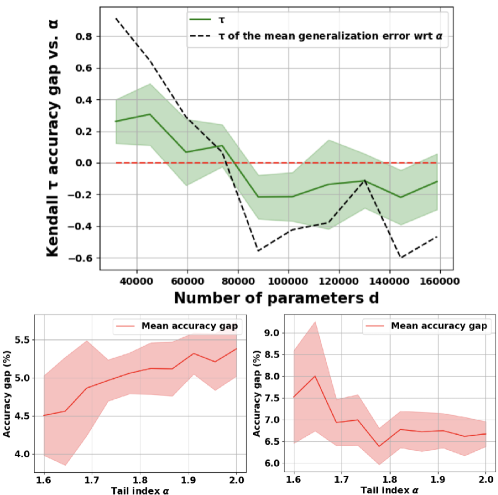
Figure 1: (up) Correlation (Kendall’s $\tau$) between $\alpha$ and the accuracy gap, for different values of $d$, with a FCN$2$ trained on MNIST. The green curve is the average $\tau$ over $10$ random seeds. The black curve is the correlation between $\alpha$ and the average accuracy gap over $10$ seeds. (bottom) Accuracy gap with respect to $\alpha$ for $d=3.10^{4}$ (left) and $d=15.10^{4}$ (right).

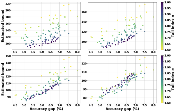
Figure 2: Bound estimated from Equation 17 versus accuracy gap for a FCN$2$ on MNIST, for different values of $R$: $1$ (top left), $3$ (top right), $7$ (bottom left), $15$ (bottom right).

Results. We test our theory through $3$ types of experiments. We present in this section their results for a FCN$2$ trained on MNIST. Section F.4 contains additional experiments.

First, on Figure 1, we compute the correlation between $\alpha$ and the accuracy gap, measured in term of a Kendall’s $\tau$ coefficient(Kendall, 1938). We use a FCN$2$ and let the width vary to compute $\tau$ for different values of the dimension $d$. The detailed procedure to obtain Figure 1 can be found in Sections F.3 and F.1. We observe that the phase transition between positive and negative correlation, predicted in Section 5, happens for a value of the dimension $d\simeq 8.10^{4}$, which we will use to further estimate $R$. We observe that the positive correlation of the heavy regime seems to be stronger than the negative correlation of the light regime.

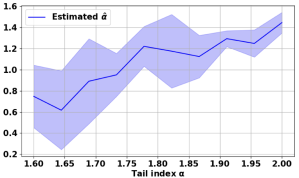
Figure 3: Regression of the tail-index $\alpha$ from the accuracy error, for a FCN$2$ trained on MNIST.

The bound of Theorem 10 is computable in practice, we estimate it by the formula (in that case $s=1/2$):

$$\widehat{G}:=\sqrt{\frac{P_{\alpha}d^{1-\frac{\alpha}{2}}\gamma}{n\sigma_{1}R^{2-\alpha}}\sum_{k=1}^{N}\left\|\nabla\widehat{F}_{S}(\widehat{W}_{k}^{S})\right\|^{2}}.$$ (17)

On Figure 2, we plot Equation 17 w.r.t. to the accuracy gap, for several values of $R$. We use $R=1$ as a default choice, as $R$ is unknown a priori, it shows, for each value of $\alpha$, a good correlation with the accuracy gap. Nonetheless, based on Figure 1, conducted with the same setting as Figure 2, we can estimate the value of $R$ to be in $\simeq[2.8,7]$. If we use these values in Equation 17, the observed correlation is much stronger. If we use a slightly larger value ($R=15$), we see, in Figure 2, that the correlation becomes almost perfect, which we interpret as the phase transition being correctly taken into account. This shows that the right corrective term in Equation 46 is indeed of the form $R^{2-\alpha}$. We note that the reason why our bound over-estimates the accuracy gap, is that it increases with $T$. However, as the bounds presented in Sections 4.3 and E are time-uniform and have similar constants and dependence on $\nabla\widehat{F}_{S}$ as in Theorem 10, we believe that this issue can be alleviated by extending Theorem 10 in a similar direction, which we leave as an open question.

Finally, to obtain Figure 3, we fixed $\sigma$ to $0.01$ and let $d$ vary in a fixed range. Based on Equation 14, we expect the accuracy error, denoted $G_{S}$, to be proportional to $d^{1/2-\alpha/4}$. This suggests to perform the linear regression, $\log(G_{S})\simeq\widehat{r}\log(d)+C,$ to compute an estimate $\widehat{\alpha}:=2-4\widehat{r}$ of the tail-index $\alpha$. The blue curve in Figure 3 shows $\widehat{\alpha}$ in terms of $\alpha$. This shows a strong correlation between the estimated and the ground-truth tail-index, in particular, we retrieve the expected monotonicity. However, $\widehat{\alpha}$ seems to underestimate the true value of $\alpha$, by a term independent of $\alpha$.

7 Conclusion

In this paper, we proved generalization bounds for heavy-tailed SDEs. Our results are the first to be both in high-probability and computable. Moreover, they allow for a more flexible setup and have a better dimension-dependence than existing works. We analyzed the constants appearing in our theorems, which led us to predict the existence of a phase transition in terms of the effect of the tail index on the generalization. We supported our theory with various numerical experiments. Several directions remain to be studied in the future. In particular, obtaining new functional inequalities, such as presented in Appendix E, could improve the time-dependence of the bounds. Moreover, understanding the interaction, between small batches and the stable noise $L_{t}^{\alpha}$, would be a natural extension of the theory.

Broader Impact Statement.

This work is largely theoretical, it does not have any direct social or ethical impact.

Organization of the appendix: The appendix starts with a short notations section. The remainder of the document is then organized as follows:

• In Appendix A, some technical background is presented. The technical background is divided into three main topics: PAC-Bayesian bounds, Lévy processes, and $\Phi$-entropies inequalities. We also include a small subsection on the Euler’s $\Gamma$ function.

• Appendix B presents the proof of our version of a PAC-Bayesian generalization bound for subgaussian losses.

• Appendix C is the core of the appendix, we prove the main result, along with all intermediary lemmas, and introduce the notations necessary to understand those proofs. Moreover, a few additional theoretical results are given, which are a refinement of the main results. In particular, the extension of the theory to a discrete setting is discussed in Section C.6, while Section C.7 presents bounds in the case $\sigma_{2}>0$, which are different than those of Section 4.1.

• In Appendix D, we provide details on how to obtain the theoretical results of Appendix D.

• In Appendix E, we discuss the time dependence of Corollaries 8 and 10 and mention that this time dependence could be largely improved by assuming that a certain class of inequality holds.

• Finally, Appendix F presents some details on the experimental setting, as well as a few additional experiments.

Notations

In order to simplify the notations, we will sometimes omit the $x$ variable when integrating with respect to the Lebesgue measure in ${\mathds{R}^{d}}$, i.e. we will write invariable $\int f$ or $\int fdx$, instead $\int f(x)dx$. These conventions are meant to ease the notations throughout the paper.

We will use the following convention regarding the Fourier transform, for $\phi:\mathds{R}^{d}\longrightarrow\mathds{R}$, regular enough, we set:

$$\mathcal{F}\phi(\xi):=\int e^{-ix\cdot\xi}\phi(x)dx.$$ (18)

The partial derivative $\partial/\partial t$ will often be shortened as $\partial_{t}$. Similarly, $\partial_{i}$ may denote $\partial/\partial x_{i}$.

Let’s also precise some notations introduced in the main part of the document. As mentioned in Section 1, the data space is denoted $\mathcal{Z}$. More precisely, $\mathcal{Z}$ is a measurable space, endowed with a $\sigma$-algebra $\mathcal{F}$. The data distribution, $\mu_{z}$, is a probability measure on $(\mathcal{Z},\mathcal{F})$.

Appendix A Technical background

A.1 Information-theoretic terms and PAC-Bayesian bounds

The concept of PAC-Bayesian analysis has been introduced in Section 2.2. In this section, we detail two particular PAC-Bayesian bounds that we use for the derivation of our main results. For a more detailed introduction to those subjects, the reader is invited to consult (Alquier, 2021).

We start by defining the information theoretic (IT) quantities appearing in the aforementioned theorems, see (van Erven and Harremoës, 2014) for more details. Let $\mu$ and $\nu$ be two probability measures, on the same space, such that $\mu$ is absolutely continuous with respect to $\nu$. We define the Kullback-Leibler (KL) divergence as:

$$\text{{{KL}}}\left(\mu||\nu\right):=\int\log\left(\frac{d\mu}{d\nu}\right)d\mu,$$ (19)

where $d\mu/d\nu$ denotes the Radon-Nykodym derivative between $\mu$ and $\nu$.

Next, we define the Renyi divergences, for some $\beta>1$, as :

$$\text{{{D}}}_{\beta}\left(\mu||\nu\right):=\frac{1}{\beta-1}\log\left(\int\left(\frac{d\mu}{d\nu}\right)^{\beta}d\nu\right).$$ (20)

By convention, we set $\text{{{D}}}_{1}\left(\cdot||\cdot\right):=\text{{{KL}}}\left(\cdot||\cdot\right)$, so that, by (van Erven and Harremoës, 2014, Theorem $3$), $\text{{{D}}}_{\beta}\left(\cdot||\cdot\right)$ is nondecreasing in $\beta$.

In the following, to mimic the notations of the rest of the paper, we consider a probability measure $\pi$ on ${\mathds{R}^{d}}$ and a family of data-dependent probability measures on ${\mathds{R}^{d}}$, $(\rho_{S})_{S\in\mathcal{Z}^{n}}$, where $\mathcal{Z}$ has been defined in Section 1. We mainly require this family to satisfy the following properties:

1. Absolute continuity: for (almost-)all $S$, we have $\rho_{S}\ll\pi$.

2. Markov kernel property, for all Borel set $B\subset{\mathds{R}^{d}}$, the map $S\longmapsto\rho_{S}(B)$ is $\mathcal{F}^{\otimes n}$-measurable. Recall that $\mathcal{F}$ is the $\sigma$-algebra on the data space $\mathcal{Z}$.

In the following, as we do in the rest of the paper, we refer to $\pi$ as a prior distribution, and to $\rho_{S}$ as posterior distributions.

The next theorem is a generic PAC-bayesian bound due to Germain et al. (2009).

Theorem 14 (General PAC-Bayesian bound)

Let $\zeta\in(0,1)$ and $\varphi:{\mathds{R}^{d}}\times\mathcal{Z}^{n}\to\mathds{R}$ a measurable function, integrable with respect to the posterior distributions. With probability at least $1-\zeta$, over $S\sim\mu_{z}^{\otimes n}$, we have:

$$\mathds{E}_{w\sim\rho_{S}}\left[\varphi(w,S)\right]\leq\log(1/\zeta)+\text{{{KL}}}\left(\rho_{S}||\pi\right)+\log\mathds{E}_{S}\mathds{E}_{w\sim\pi}\left[e^{\varphi(w,S)}\right],$$

where the KL divergence has been defined by Equation 19.

Theorem 15 (Disintegrated PAC-Bayesian bound)

Let $\zeta\in(0,1)$ and $\varphi:{\mathds{R}^{d}}\times\mathcal{Z}^{n}\to\mathds{R}$ a measurable function. With probability at least $1-\zeta$, over $S\sim\mu_{z}^{\otimes n}$ and $w\sim\rho_{S}$, we have:

$$\frac{\beta}{\beta{-}1}\varphi(w,S)\leq\frac{2\beta-1}{\beta-1}\log(2/\zeta)+\text{{{D}}}_{\beta}\left(\rho_{S}||\pi\right)+\log\mathds{E}_{S}\mathds{E}_{w\sim\pi}\left[e^{\frac{\beta}{\beta-1}\varphi(w,S)}\right],$$

where the Renyi divergence has been defined by Equation 20.

We give below one particular instance of Theorem 14, using the notations introduced in Section 1, for $\mu_{z}$, $S$, $f$, $L$ and $\widehat{L}_{S}$. This theorem was first proven by (McAllester, 2003; Maurer, 2004).

Theorem 16

Assume that the objective $f$ is bounded in $[0,1]$, then, with probability at least $1-\zeta$ over $S\sim\mu_{z}^{\otimes n}$, we have:

$$\mathds{E}_{\rho_{S}}\left[L(w)-\widehat{L}_{S}(w)\right]\leq\sqrt{\frac{\text{{{KL}}}\left(\rho_{S}||\pi\right)+\log\frac{2\sqrt{n}}{\zeta}}{2n}}.$$

A.2 Background on Levy processes and associated pseudo-differential operators

In this section, we introduce some basic notions related to the study of Lévy process. In particular, we insist on the case of stable Lévy processes and their associated operators, namely the Laplacian and fractional Laplacian. Therefore, we make the link between the SDE (3) and the PDE (6) as clear as possible for the reader. We will also set up several notations used throughout the sequel.

A.2.1 Levy processes

In this subsection, we recall some basic notions related to Lévy process, in order to make our main results as clear as possible. The main goal is to get an understanding of Equation 6. For a more detailed introduction to those subjects, we refer the reader to (Schilling, 1998; Xiao, 2004; Böttcher et al., 2013).

Definition 17 (Lévy process)

A Lévy process $(L_{t})_{t\geq 0}$, in ${\mathds{R}^{d}}$, is a stochastic process such that:

• $L_{0}=0$,

• the increments are independents, i.e., for all $t_{1}<\dots<t_{K}$, the processes $L_{t_{i}}-L_{t_{i-1}}$ are independent,

• the increments are stationary, i.e. for $0\leq s<t$, we have $L_{t}-L_{s}\overset{\mathbf{d}}{=}L_{s}$, where $\overset{\mathbf{d}}{=}$ denotes the equality in distribution,

• the process is stochastically continuous, by which we mean that for any $s\geq 0$ and $\delta>0$, we have:

  $$\lim_{t\to s}\mathds{P}\left(\left\|L_{t}-L_{s}\right\|>\delta\right)=0.$$

Equivalently, one can show that stochastic continuity is equivalent to the process having a modification with cadlag paths, therefore, the paths of Lévy processes may exhibit jumps.

Levy processes are closely related to the notion of infinitely divisible distributions. A probability distribution is said to be infinitely divisible if, for any $N\in\mathds{N}^{\star}$, it can be seen that $F$ is the distribution of the sum of $N$ random variables.

Lévy processes have infinitely divisible distributions. Following Schilling and Schnurr (2010, Corollary $2.5$), it can be deduced that their characteristic function can be expressed as (with $\xi\in{\mathds{R}^{d}}$):

$$\mathds{E}\left[e^{i\xi\cdot L_{t}}\right]=e^{-t\psi(\xi)},$$

where the function $\psi$ is called the characteristic exponent. It characterizes the Lévy process $(L_{t})$ and plays a great role in our analysis.

The following theorem is the fundamental result in the study of characteristic exponents. In particular, it introduces the notion of Lévy measure, which we use repeatedly. Several conventions or notations may exist for this formula, we follow those of (Böttcher et al., 2013, Theorem $2.2$).

Theorem 18 (Lévy-Khintchine formula)

Let $(L_{t})_{t\geq 0}$ be a Lévy process as above. The characteristic exponent of $L$ has the following form:

$$\forall\xi\in{\mathds{R}^{d}},\leavevmode\nobreak\ \psi(\xi)=-il\cdot\xi+\frac{1}{2}\xi\cdot Q\xi+\int_{{\mathds{R}^{d}}\backslash\left\{0\right\}}\left(1-e^{iz\cdot\xi}+i\xi\cdot z\chi(\left\|z\right\|)\right)d\nu(z),$$

where $l\in{\mathds{R}^{d}}$, $Q\in\mathds{R}^{d\times d}$ is a symmetric positive semi-definite matrix and $\nu$ is a positive measure on ${\mathds{R}^{d}}\backslash\left\{0\right\}$ such that

$$\int_{{\mathds{R}^{d}}\backslash\left\{0\right\}}\min(1,\left\|z\right\|^{2})d\nu(z)<+\infty.$$

Finally, $\chi$ is a truncation function, such that $\chi(s)$ and $s\chi(s)$ are bounded and there exists a constant $\kappa>0$ such that $0\leq 1-\chi(s)\leq\kappa\min(1,s)$.

The triplet $(l,Q,\nu)$ is called the Lévy triplet associated to $L$, and $\nu$ is the Lévy measure.

Remark 19

As it is mentioned in (Böttcher et al., 2013, Theorem $2.2$), the truncation function $\chi$ is arbitrary and only influences the drift $l\in{\mathds{R}^{d}}$. In our paper, we only consider Lévy process and infinitely divisible distributions with no drift (i.e. $l=0$), the choice of $\chi$ therefore has no impact. A typical choice would be $\chi(s)=\min(1,s^{2})$.

Remark 20

It is clear, from the above discussion, that any infinitely divisible distribution can be associated with a Lévy triplet, as in Theorem 18.

Example 1 (Brownian motion)

The Lévy triplet $(0,I_{d},0)$ corresponds to the standard Brownian motion in ${\mathds{R}^{d}}$, denoted $(B_{t})_{t\geq 0}$.

We end this subsection by defining stable Lévy processes, which are the main object of our study, see (Böttcher et al., 2013, Example $2.4.d$).

Definition 21 (Stable Lévy processes)

Let $\alpha\in(0,2]$, the (isotropic) $\alpha$-stable Lévy process $(L_{t}^{\alpha})_{t\geq 0}$, is defined by the following expression of its characteristic exponent: $\psi(\xi)=normof{\xi}^{\alpha}$. Its Lévy triplet is given by:

• If $\alpha=2$, then the triplet is $(0,2I_{d},0)$, in which case we have $L_{t}^{2}=\sqrt{2}B_{t}$.

• If $\alpha\in(0,2)$, the triplet is $(0,0,\nu_{\alpha})$, with:

  $$d\nu_{\alpha}(z):=C_{\alpha,d}\frac{dz}{\left\|z\right\|^{d+\alpha}},\quad C_{\alpha,d}:=\alpha 2^{\alpha-1}\pi^{-d/2}\frac{\Gamma\left(\frac{\alpha+d}{2}\right)}{\Gamma\left(1-\frac{\alpha}{2}\right)}.$$ (21)

A.2.2 Generator of the semigroup and fractional Laplacian

In this subsection, we introduce the notion of fractional Laplacian. This is related to the study of Lévy processes through the notion of ”infinitesimal generator of the semigroup”, which we first define.

Given a temporally homogeneous Markov process $(X_{t})_{t\geq 0}$ we define its semigroup $(P_{t})_{t\geq 0}$ (Xiao, 2004; Schilling, 2016), as the following operators, defined for bounded measurable function $f$:

$$P_{t}f(x)=\mathds{E}^{x}[f(X_{t})],$$

where $\mathds{E}^{x}$ denotes the initialization of the process at $x$ (i.e. conditionally on $X_{0}=x$).

If $X$ is a Lévy process, or more generally a Feller process, see (Schilling, 2016), such a semigroup is characterized by its infinitesimal generator.

Definition 22

Let $\mathcal{C}^{0}_{\infty}({\mathds{R}^{d}})$ be the space of continuous functions vanishing to zero at infinity. As soon as it exists, we define the generator of the semigroup $(P_{t})_{t}$ as the ensuing limit:

$$Af(x):=\lim_{t\to 0}\frac{P_{t}f-f}{t},$$

where the limit is understood in the uniform norm on $\mathcal{C}^{0}_{\infty}({\mathds{R}^{d}})$. The domain of the generator, denoted $\mathcal{D}(A)\subset\mathcal{C}^{0}_{\infty}({\mathds{R}^{d}})$, is the set of functions for which the above limit is defined.

It is known that the generator of $L_{t}^{2}=\sqrt{2}B_{t}$ is $A\phi=\Delta\phi$, where $\Delta$ denotes the Laplacian. Following (Böttcher et al., 2013; Duan, 2015; Umarov et al., 2018), we can express the generator of $(L_{t}^{\alpha})$, for $\alpha\in(0,2)$, on the appropriated domain, which at least contains $\mathcal{C}_{c}^{\infty}({\mathds{R}^{d}})$,

$$A\phi(x)=C_{\alpha,d}\int_{{\mathds{R}^{d}}}\left(\phi(x+z)-\phi(x)-\nabla\phi(x)\cdot z\chi(\left\|z\right\|)\right)d\nu_{\alpha}(z),$$ (22)

with the same notations as in Definition 21. Following (Lischke et al., 2019; Umarov et al., 2018), Equation 22 is one of the possible equivalent definitions of the fractional Laplacian. Note that the term fractional Laplacian is actually an abuse of notations, the correct terminology would be the negative fractional negative Laplacian, as we can see in the following definition:

$$-\left(-\Delta\right)^{\frac{\alpha}{2}}\phi(x):=C_{\alpha,d}\int_{{\mathds{R}^{d}}}\left(\phi(x+z)-\phi(x)-\nabla\phi(x)\cdot z\chi(\left\|z\right\|)\right)d\nu_{\alpha}(z),$$ (23)

Remark 23 (Equivalent definitions of $\left(-\Delta\right)^{\frac{\alpha}{2}}$)

There are several equivalent definitions of the fractional Laplacian, we refer the reader to (Lischke et al., 2019; Teymurazyan, 2023) for all details. We only mention two that are commonly used:

• Principal value integral this is the definition used by Raj et al. (2023b), even though their sign convention is different:

  $$\left(-\Delta\right)^{\frac{\alpha}{2}}\phi(x)=C_{\alpha,d}\lim_{\epsilon\to 0}\int_{{\mathds{R}^{d}}\backslash B_{\epsilon}(0)}\frac{u(x)-u(x+z)}{\left\|z\right\|^{d+\alpha}}dz.$$

• Fourier transform representation: $\mathcal{F}(\left(-\Delta\right)^{\frac{\alpha}{2}}\phi)(\xi)=\left\|\xi\right\|^{\alpha}\mathcal{F}\phi(\xi)$.

A.2.3 Lévy-driven diffusions

In this subsection, we consider a function $V:{\mathds{R}^{d}}\longrightarrow\mathds{R}$, which we call potential function. We consider the following stochastic differential equation (SDE):

$$dX_{t}=-\nabla V(X_{t})dt+\sigma_{1}dL_{t}^{\alpha}+\sigma_{2}\sqrt{2}dB_{t},$$ (24)

with $\alpha\in(0,2)$. This equation admits a strong solution (in the Itô sense), as soon as $V$ is smooth, i.e. it satisfies 4, see (Schilling and Schnurr, 2010).

Let us denote by $\rho=\rho(t,x)$ the probability density of the process $X$. Under certain regularity conditions, this function $\rho$ is known to satisfy the following Fokker-Planck equation, at least in a weak sense (i.e. in the sense of distributions):

$$\partial_{t}\rho=\nabla\cdot(\rho\nabla V)+I\left[\rho\right],$$ (25)

with the operator $\rho$ being defined using the self adjoint operator of the driving process of Equation 24 as:

$$I\left[\rho\right]=\sigma_{2}^{2}\Delta\rho+C_{\alpha,d}\sigma_{1}^{\alpha}\int\left(\rho(x+z)-\rho(x)-\nabla\rho(x)\cdot z\xi(\left\|z\right\|)\right)d\nu_{\alpha}(z),$$ (26)

Equation 25 is exactly Equation 6, with $V=F_{S}$.

We will use the self-adjointness of such an operator, recalled in the following lemma, of which the reader may find more precise formulations in (Gentil and Imbert, 2008; Lischke et al., 2019; Tristani, 2013).

Lemma 24

As soon as it is well defined, the operator $I$, defined by Equation 26 is self adjoint, i.e. for $\varphi$ and $\psi$, regular enough, we have:

$$\int\varphi I\left[\psi\right]dx=\int\psi I\left[\varphi\right].$$

We now discuss the validity of this equation in the following two remarks. Those remarks may be skipped without hurting the general understanding of the paper. They are meant to explain what needs to be assumed to be as rigorous as possible in our treatment of the fractional Fokker-Planck equation.

Remark 25 (Justification of the equation)

Using the main result of Kühn (2018), it can be argued that, under 4, $X$ is a Feller process. Its generator can be expressed as (Schilling and Schnurr, 2010; Duan, 2015; Umarov et al., 2018):

$$A\phi(x)=-\nabla V(x)\cdot\nabla\phi(x)+\sigma_{2}^{2}\Delta\phi(x)-\sigma_{1}^{\alpha}\left(-\Delta\right)^{\frac{\alpha}{2}}\phi(x).$$

If we denote by $(P_{t})_{t}$ the semi-group associated with $X$, then we have the Kolmogorov backward equation, for $f$ in the generator $\mathcal{D}(A)$ of $A$:

$$\frac{d}{dt}P_{t}f=AP_{t}f=P_{t}Af,$$

taking the $L^{2}$-adjoint of this equation leads to $\partial_{t}\rho=A^{\star}\rho$ (at least in a weak sense). A direct computation of the adjoint $A^{\star}$, using properties of the fractional Laplacian, leads to Equation 25.

Remark 26 (Validity of Equation 25)

Let us quickly discuss the domain of validity of the Fokker-Planck equations considered in this paper. We are in particular interested in the (local) regularity of the potential solutions, as they are necessary to give meaning to several computations made in our proofs. Let us first mention that in the simpler case of a quadratic potential, the regularity easily comes from the analytic solution of such equations (Lafleche, 2020). Moreover, equations such as Equation 25 are known to have regularization properties and have the ability to generate smooth solutions.

More precisely, as it is mentioned in (Umarov et al., 2018), under regularity assumptions, it is known that such an equation is satisfied in a weak sense, namely in the sense of distributions (Halperin and Schwartz, 1952). Therefore, one may ask whether smooth solutions do actually exist. Smoothness in the $x$ variable has been proven for the Ornstein-Uhlenbeck drift by (Xie et al., 2015). Space-time regularity has been proven in (Imbert, 2005) in the case of a bounded force field $\nabla F_{S}$. An example of space regularity was achieved in the case of a force field with bounded derivatives of positive order, in (Wang and Duan, 2017). Finally, let us mention the work of (Lafleche, 2020), which provides further regularity conditions.

A.3 Logarithmic Sobolev inequalities and $\Phi$-entropy inequalities

Logarithmic Sobolev inequalities (LSI) and Poincaré inequalities are central tools in probability theory. LSIs were historically introduced by Gross (1975) and have famously been applied to the analysis of Markov processes (Bakry et al., 2014), the study of evolution equations (Markowich and Villani, 2004), and have been connected to optimal transport and geometry (Villani, 2009). For a short introduction, the reader may consult the tutorials (Chafai, 2004; Chafai and Lehec, 2017). In this section, we quickly introduce a few of these results, with an emphasis on a generalization to infinitely divisible distributions, playing an important role in our study.

A.3.1 The classical inequalities

We first quickly recall the classical Poincaré inequality and LSI. They hold for the standard Gaussian measure, defined by $\gamma_{d}=\mathcal{N}(0,I_{d})$. We first give Poincaré inequality:

Theorem 27

Let $f$ be a function such that $\nabla f\in L^{2}(\gamma_{d})$, we have:

$$\int_{\mathds{R}^{d}}f^{2}d\gamma_{d}-\left(\int_{\mathds{R}^{d}}fd\gamma_{d}\right)^{2}\leq\int_{\mathds{R}^{d}}\left\|\nabla f\right\|^{2}d\gamma_{n}.$$

Example 2

If we define the convex function $\Phi(x)=\Phi_{2}(x):=\frac{x^{2}}{2}$, as in Section 4.3, then the left hand side of the inequality of Theorem 27 can be understood as $2\text{Ent}_{\gamma_{d}}^{\Phi}\left(f\right)$.

The next theorem is the classical LSI for the Gaussian measure $\gamma_{d}$:

Theorem 28

Let $f\in\mathcal{C}^{1}({\mathds{R}^{d}},R)$ be non-negative and integrable, then we have, for $\Phi(x)=\Phi_{\log}(x)=x\log(x)$:

$$\text{Ent}_{\gamma_{d}}^{\Phi}\left(f\right)\leq\frac{1}{2}\int_{\mathds{R}^{d}}\frac{\left\|\nabla f\right\|^{2}}{f}d\gamma_{d}.$$

Example 3

With the convex function $\Phi$ used in the above theorem, the right-hand side of the inequality is, up to the constant, the Fisher information, which we call $\Phi$-information in Lemma 7.

A.3.2 Generalization to infinitely divisible distributions

Part of our analysis is based on a generalization of those inequalities to infinitely divisible distributions. Let us recall that those distributions have been defined in Section A.2 and can be equivalently seen as the distribution of Lévy processes. This is how we connect those inequalities to our theory.

Let us first recall the definition of $\Phi$-entropies, i.e. Definition 2.

See 2

Note that, by Jensen’s inequality, such a term is always non-negative.

The following theorem was proved by Wu (2000) and Chafai (2004), it generalizes Poincaré and logarithmic Sobolev inequalities to infinitely divisible distributions.

Theorem 29 (Generalized LSI)

Let $\mu$ be an infinitely divisible law on ${\mathds{R}^{d}}$, with associated triplet denoted $(b,Q,\nu)$, in the sense of Theorem 18, then, for every smooth enough function $v$, we have:

$$\text{Ent}_{\bar{u}_{\infty}}^{\Phi}\left(v\right)\leq\frac{1}{2}\int\Phi^{\prime\prime}(v)\nabla v\cdot Q\nabla v\leavevmode\nobreak\ d\mu+\iint D_{\Phi}(v(x+z),v(x))d\nu(z)d\mu(x).$$

Note that, when $\mu=\gamma_{d}$, then its Lévy triplet is $(0,I_{d},0)$, so that Theorem 29 implies Theorems 27 and 28.

A.4 Some properties of the Gamma function

The Euler gamma function is classically defines by:

$$\forall x>0,\leavevmode\nobreak\ \Gamma(x)=\int_{0}^{\infty}t^{x-1}e^{-t}dt.$$

It has a natural extension to $\mathds{C}\backslash(-\mathds{N})$. In this subsection, we give a few properties of this function, which will be useful to prove the results of Section 5 in Appendix D.

One particular value:

$$\Gamma\left(\frac{1}{2}\right)=\sqrt{\pi}.$$

Lemma 30 (Euler’s reflection formula)

For all $z\in\mathds{R}\backslash\mathds{Z}$, we have:

$$\Gamma(1-z)\Gamma(z)=\frac{\pi}{\sin(\pi z)}.$$

Lemma 31 (Stirling’s formulas)

We have have the two following asymptotic formulas:

$$\Gamma(x+1)\underset{x\to\infty}{\sim}\sqrt{2\pi x}\left(\frac{x}{e}\right)^{x},$$

and, for all $\alpha\in\mathds{R}$:

$$\Gamma(x+\alpha)\underset{x\to\infty}{\sim}\Gamma(x)x^{\alpha}.$$

Appendix B A PAC-Bayesian bound for sub-gaussian losses

In this section, we give proof of a PAC-Bayesian bound, which applies to sub-gaussian losses. The notations for $\mathcal{Z}$, $S$, $\mu_{z}$, $\ell$, $L$ and $\widehat{L}_{S}$ are the same as in Section 1, i.e.:

$$L(w):=\mathds{E}_{z\sim\mu_{z}}\left[\ell(w,z)\right],\quad,\widehat{L}_{S}(w):=\frac{1}{n}\sum_{i=1}^{n}\ell(w,z_{i}),$$

with $S=(z_{1},\dots,z_{n})\in\mathcal{Z}^{n}$. We consider a prior distribution $\pi$ as well as a family of posterior distributions, as it has been introduced in Section A.1.

By Theorem 16, which has been proven by McAllester (2003); Maurer (2004), we know that with probability at least $1-\zeta$ under $S\sim\mu_{z}^{\otimes n}$, we have:

$$\mathds{E}_{\rho_{S}}\left[L(w)-\widehat{L}_{S}(w)\right]\leq\sqrt{\frac{\text{{{KL}}}\left(\rho_{S}||\pi\right)+\log\frac{2\sqrt{n}}{\zeta}}{2n}}.$$

Unfortunately, to the best of our knowledge, no such bounds (i.e. without the variable $\lambda$ like in Theorems 14 and 15), exist for sub-gaussian losses, which is the assumption we make in our paper. As an additional theoretical contribution, we present the following PAC-Bayesian bound for sub-gaussian losses. We believe it may be useful for other works.

Theorem 32

We assume that $f$ is $s^{2}$-subgaussian, in the sense of 3. Then, with probability at least $1-\zeta$ under $S\sim\mu_{z}^{\otimes n}$, we have:

$$\mathds{E}_{\rho_{S}}\left[L(w)-\widehat{L}_{S}(w)\right]\leq 2s\sqrt{\frac{\text{{{KL}}}\left(\rho_{S}||\pi\right)+\log\frac{3}{\zeta}}{n}}.$$

Proof  The proof follows very closely that of (Vershynin, 2020, Proposition $2.5.2$), which we adapt to our particular case to exhibit the exact absolute constants.

We start by fixing $0<a<1/(2s^{2})$ and applying Theorem 14 to the function $\phi(w,S):=an\left(L(w)-\widehat{L}_{S}(w)\right)^{2}$, which gives that, with probability at least $1-\zeta$ under $S\sim\mu_{z}^{\otimes n}$:

$$an\mathds{E}_{\rho_{S}}\left[\left(L(w)-\widehat{L}_{S}(w)\right)^{2}\right]\leq\text{{{KL}}}\left(\rho_{S}||\pi\right)+\log(1/\zeta)+\log\mathds{E}_{\pi}\mathds{E}_{S}\left[e^{an\left(L(w)-\widehat{L}_{S}(w)\right)^{2}}\right].$$

The above holds as soon as the last term is defined and finite, this will be an outcome of our computations. Let us denote $\Delta:=|L(w)-\widehat{L}_{S}(w)|$ and estimate the expected exponential term, by Tonelli’s theorem:

$$\mathds{E}_{S}\left[e^{an\Delta^{2}}\right]=1+\sum_{k=1}^{\infty}\frac{a^{k}n^{k}}{k!}\mathds{E}_{S}\left[\Delta^{2k}\right].$$

Let us fix some $p>1$, we note that we have:

$$\mathds{E}_{S}\left[\Delta^{p}\right]=\int_{0}^{\infty}\mathds{P}\left(\Delta^{p}\geq\epsilon\right)d\epsilon$$

Now, by Hoeffding’s inequality and several changes of variables, we have:

$$\mathds{E}_{S}\left[\Delta^{p}\right] \leq\int_{0}^{\infty}\mathds{P}\left(\Delta\geq\epsilon^{1/p}\right)d\epsilon$$

$$\leq 2\int_{0}^{\infty}e^{-\frac{n\epsilon^{2/p}}{2s^{2}}}d\epsilon$$

$$=p\int_{0}^{\infty}e^{-\frac{nv}{2s^{2}}}v^{\frac{p}{2}-1}dv$$

$$=p\left(\frac{2s^{2}}{n}\right)^{p/2}\int_{0}^{\infty}e^{-t}t^{\frac{p}{2}-1}dt$$

$$=p\left(\frac{2s^{2}}{n}\right)^{p/2}\Gamma\left(\frac{p}{2}\right)$$

$$=2\left(\frac{2s^{2}}{n}\right)^{p/2}\Gamma\left(1+\frac{p}{2}\right),$$

were the last two inequalities follow from the definition and properties of the $\Gamma$ function, as stated in Section A.4. If we plug this into our previous computations, we find that:

$$\mathds{E}_{S}\left[e^{an\Delta^{2}}\right] \leq 1+2\sum_{k=1}^{\infty}\left(\frac{2s^{2}}{n}\right)^{k}\frac{a^{k}n^{k}}{k!}k!$$

$$\leq 1+2\sum_{k=1}^{\infty}(2s^{2}a)^{k}$$

$$=1+2\frac{2s^{2}a}{1-2s^{2}a},$$

where the last line holds because we assumed $2as^{2}<1$. We now make the following particular choice $a:=1/(4s^{2})$ and we get:

$$\mathds{E}_{S}\left[e^{an\Delta^{2}}\right]\leq 3.$$

Now, by Jensen’s inequality and Fubini’s theorem, this implies that, with probability at least $1-\zeta$ over $S\sim\mu_{z}^{\otimes n}$:

$$\frac{n}{4s^{2}}\mathds{E}_{\rho_{S}}\left[L(w)-\widehat{L}_{S}(w)\right]^{2}\leq\text{{{KL}}}\left(\rho_{S}||\pi\right)+\log(1/\zeta)+\log(3),$$

which immediately implies the desired result.  

Remark 33

If we assume, as in Theorem 16, that the function $f$ is bounded in $[0,1]$, then, by Hoeffding’s lemma, $f$ is $s^{2}$-subgaussian with $s=1/2$. Therefore, our bound implies:

$$\mathds{E}_{\rho_{S}}\left[L(w)-\widehat{L}_{S}(w)\right]\leq\sqrt{\frac{\text{{{KL}}}\left(\rho_{S}||\pi\right)+\log\frac{3}{\zeta}}{n}},$$

which has a slightly less good constant than Theorem 16, but we improve the term $\log(2\sqrt{n})$ into $\log(3)$.

By combining the previous computations with the disintegrated bound of Theorem 15, we immediately obtain:

Theorem 34

We assume that $f$ is $s^{2}$-subgaussian, in the sense of 3. Then, with probability at least $1-\zeta$ under $S\sim\mu_{z}^{\otimes n}$ and $w\sim\rho_{S}$, we have:

$$L(w)-\widehat{L}_{S}(w)\leq 2s\sqrt{\frac{\text{{{D}}}_{2}\left(\rho_{S}||\pi\right)+\log\frac{24}{\zeta^{3}}}{n}}.$$

Appendix C Proofs of the main theorems and additional results

In all the proofs, we use the following notation:

$$I\left[u\right]=\sigma_{2}^{2}\Delta u+C_{\alpha,d}\sigma_{1}^{\alpha}\int\left(u(x+z)-u(x)-\nabla u(x)\cdot z\xi(\left\|z\right\|)\right)d\nu_{\alpha}(z),$$

Note that this is the generator of the process driving Equation 3, e.g. $\sigma_{2}B_{t}+\sigma_{1}L_{t}^{\alpha}$. We will use the following notations for the drift terms:

$$V_{S}(w)=\widehat{F}_{S}(w)+\frac{\eta}{2}\left\|w\right\|^{2},\quad\quad V(w)=\frac{\eta}{2}\left\|w\right\|^{2}.$$

We use the notations $u_{t}^{S},\bar{u}_{\infty},\rho_{t}^{S},\pi$ and $v_{t}^{S}$ in the same way as they have been introduced in Section 2. Moreover, we remind the reader that we often denote $v$ instead of $v_{t}^{S}$, and $u$ instead of $u^{S}_{t}$, the dependence in the time $t$ and the data $S$ being implicit.

C.1 The main decomposition

Before proving our main results, we define the Bregman divergence, associated with a convex function $\Phi$. We will use it repeatedly in our proofs and statements. This notion also justifies that we call the term $B_{\Phi}^{\alpha}$, appearing in Lemma 7, the ”Bregman” integral.

Definition 35

Given a convex interval $I$ and $\Phi:I\longrightarrow\mathds{R}$ a convex function, we define the Bregman divergence as:

$$D_{\Phi}(a,b):=\Phi(a)-\Phi(b)-\Phi^{\prime}(b)(a-b).$$

We first prove Lemma 7, which is the main decomposition that we use, in order to derive our main results. This result follows the computations of Gentil and Imbert (2008), which are adapted to the comparison of two dynamics.

See 7

Before proving this theorem, let us give the complete expression of the Bregman term $B_{\Phi}^{\alpha}(v)$. It is given by the following formula:

$$B_{\Phi}^{\alpha}(v)=C_{\alpha,d}\iint D_{\Phi}(v(x),v(x+z))\bar{u}_{\infty}d\nu_{\alpha}(z)dx.$$

Proof  In all the proof, we omit the time dependence of $u$ and $v$, as already mentioned above. Let us first recall the Fokker-Planck equation satisfied by $u$. Rewritten with the notations of this section, this equation is:

$$\partial_{t}u=I\left[u\right]+\nabla\cdot(u\nabla V_{S}).$$

Similarly, the stationary Fokker-Planck equation satisfied by $\bar{u}_{\infty}$ is:

$$0=I\left[\bar{u}_{\infty}\right]+\nabla\cdot(\bar{u}_{\infty}\nabla V).$$

We finally remind the reader that $v:=u/\bar{u}_{\infty}$. Using the definition of $v$ and the FPE of $u$ and $\bar{u}_{\infty}$, we have:

$$\partial_{t}v =\frac{1}{\bar{u}_{\infty}}\left(I\left[\bar{u}_{\infty}v\right]+\nabla\cdot(\bar{u}_{\infty}v\nabla V_{S})\right)$$

$$=\frac{1}{\bar{u}_{\infty}}\left(I\left[\bar{u}_{\infty}v\right]+\nabla\cdot(\bar{u}_{\infty}v\nabla V)\right)+\frac{1}{\bar{u}_{\infty}}\nabla\cdot(\bar{u}_{\infty}v\nabla(V_{S}-V))$$

Therefore, the entropy flow is equal to:

$$\frac{d}{dt}\text{Ent}_{\bar{u}_{\infty}}^{\Phi}\left(v\right) =\frac{d}{dt}\int\Phi(v)\bar{u}_{\infty}$$

$$=\int\Phi^{\prime}(v)\bar{u}_{\infty}\partial_{t}vdx$$

$$=\int\Phi^{\prime}(v)\left(I\left[\bar{u}_{\infty}v\right]+\nabla\cdot(\bar{u}_{\infty}v\nabla V)\right)dx+\int\Phi^{\prime}(v)\nabla\cdot(\bar{u}_{\infty}v\nabla(V_{S}-V))dx$$

$$=:A_{1}+A_{2}.$$

Note that the derivation under the integral is perfectly justified, from our $\Phi$-regularity assumption.

Using the self-adjointness of $I$ (see Section A.2) and the integration by parts formula, we have:

$$A_{1}=\int I\left[\Phi^{\prime}(v)\right]v\bar{u}_{\infty}dx-\int\Phi^{\prime\prime}(v)v\bar{u}_{\infty}\nabla v\cdot\nabla Vdx.$$

Now we use the formula $r\Phi^{\prime\prime}(r)=(r\Phi^{\prime}(r)-\Phi(r))^{\prime}$ and get:

$$A_{1} =\int I\left[\Phi^{\prime}(v)\right]v\bar{u}_{\infty}dx+\int(v\Phi^{\prime}(v)-\Phi(v))\nabla\cdot\bar{u}_{\infty}\nabla Vdx$$

$$=\int I\left[\Phi^{\prime}(v)\right]v\bar{u}_{\infty}dx-\int(v\Phi^{\prime}(v)-\Phi(v))I\left[\bar{u}_{\infty}\right]dx$$

$$=\int\left(I\left[\Phi^{\prime}(v)\right]v-I\left[v\Phi^{\prime}(v)\right]+I\left[\Phi(v)\right]\right)\bar{u}_{\infty}dx.$$

Therefore, we have to compute the quantity $f(v):=I\left[\Phi^{\prime}(v)\right]v-I\left[v\Phi^{\prime}(v)\right]+I\left[\Phi(v)\right]$. Using the definition of $I$, we get:

$$f(v)=\sigma_{2}^{2} \left(v\Delta\Phi^{\prime}(v)-\Delta(v\Phi^{\prime}(v))+\Delta\Phi(v)\right)$$

$$+ C_{\alpha,d}\sigma_{1}^{\alpha}\int\big{\{}v(x)\Phi^{\prime}(v(x+z))-v(x)\Phi^{\prime}(v(x))-v(x)\nabla\Phi^{\prime}(v(x))\cdot z\chi(\left\|z\right\|)$$

$$-v(x+z)\Phi^{\prime}(v(x+z))+v(x)\Phi^{\prime}(v(x))+\nabla(v\Phi^{\prime}(v))(x))\cdot z\chi(\left\|z\right\|)$$

$$+\Phi(v(x+z))-\Phi(v(x))-\nabla(\Phi(v))(x)\cdot z\chi(\left\|z\right\|)\big{\}}d\nu_{\alpha}(z).$$

which is equal, after easy computations, to:

$$f(v)=-\sigma_{2}^{2}\Phi^{\prime\prime}(v)\left\|\nabla v\right\|^{2}-C_{\alpha,d}\sigma_{1}^{\alpha}\int D_{\Phi}(v(x),v(x+z))d\nu_{\alpha}(z).$$

Therefore:

$$A_{1}=-\sigma_{2}^{2}\int\Phi^{\prime\prime}(v)\left\|\nabla v\right\|^{2}\bar{u}_{\infty}dx-C_{\alpha,d}\sigma_{1}^{\alpha}\iint D_{\Phi}(v(x),v(x+z))\bar{u}_{\infty}d\nu_{\alpha}(z)dx.$$

for the second term, we have:

$$A_{2} =\int\Phi^{\prime}(v)\nabla\cdot(\bar{u}_{\infty}v\nabla(V_{S}-V))dx$$

$$=-\int\Phi^{\prime\prime}(v)v\bar{u}_{\infty}\nabla v\cdot\nabla(V_{S}-V)dx.$$

The result follows.  

In the sequel, the quantity $\frac{d}{dt}\text{Ent}_{\bar{u}_{\infty}}^{\Phi}\left(v\right)$ will be called entropy flow.

Remark 36

If, in Equations (6) and (7), we where using the multifractal process, $\sigma\sqrt{2}dB_{t}+\sum_{i=1}^{N}\sigma_{i}L_{t}^{\alpha_{i}}$, instead of $\sqrt{2}\sigma_{2}B_{t}+\sigma_{1}L_{t}^{\alpha}$, then the result would become:

$$\frac{d}{dt}\text{Ent}_{\bar{u}_{\infty}}^{\Phi}\left(v\right)=-\sigma^{\alpha}\int\frac{\left\|\nabla v\right\|^{2}}{v}\bar{u}_{\infty}dx -\sum_{i=1}^{N}C_{\alpha_{i},d}\sigma_{i}^{\alpha_{i}}\iint D_{\Phi}(v(x),v(x+z))\bar{u}_{\infty}d\nu_{\alpha_{i}}(z)dx$$

$$-\int\nabla v\cdot\nabla\widehat{F}_{S}\bar{u}_{\infty}.$$

C.2 Proof of Corollary 8

An easy consequence of Lemma 7 is the following generalization bound, namely Corollary 8, which was first stated in Section 4.1. It holds only when $\sigma_{2}>0$.

See 8

Proof  We set $\Phi(u)=u\log(u)$, so that we have $\Phi^{\prime\prime}(u)=1/u$ and, if $v=u/\bar{u}_{\infty}$:

$$\text{Ent}_{\bar{u}_{\infty}}^{\Phi}\left(v\right)=\text{{{KL}}}\left(\rho_{S}^{t}||\pi\right).$$

Therefore, by Theorem 7, we have:

$$\frac{d}{dt}\text{{{KL}}}\left(\rho_{S}^{t}||\pi\right)=-\sigma_{2}^{2}\int\frac{\left\|\nabla v\right\|^{2}}{v}\bar{u}_{\infty}dx -C_{\alpha,d}\sigma_{1}^{\alpha}\iint D_{\Phi}(v(x),v(x+z))\bar{u}_{\infty}d\nu_{\alpha}(z)dx$$

$$+\int\nabla v\cdot\nabla(V-V_{S})\bar{u}_{\infty}.$$

Using the non-negativity of the Bregman divergence of the convex function $\Phi$, along with Cauchy-Schwarz and Young’s inequalities, we have, for any constant $C>0$:

$$\frac{d}{dt}\text{{{KL}}}\left(\rho_{S}^{t}||\pi\right)\leq-\sigma_{2}^{2}\int\frac{\left\|\nabla v\right\|^{2}}{v}\bar{u}_{\infty}dx+\frac{C}{2}\int\frac{\left\|\nabla v\right\|^{2}}{v}\bar{u}_{\infty}dx+\frac{1}{2C}\int\left\|\nabla V-\nabla V_{S}\right\|^{2}u$$

Note that Assumptions 5 and 6 ensure that the above integrals are finite.

By choosing $C=2\sigma_{2}^{2}$ and using the definition of $u$ and $\rho_{S}^{t}$, we then have, with $\Lambda:=\text{{{KL}}}\left(\rho_{S}^{0}||\pi\right)=\text{{{KL}}}\left(\rho_{0}||\pi\right)$:

$$\text{{{KL}}}\left(\rho_{S}^{t}||\pi\right)\leq\Lambda+\frac{1}{4\sigma^{2}}\int_{0}^{t}\mathds{E}_{\rho_{S}^{u}}\left[\left\|\nabla V(w)-\nabla V_{S}(w)\right\|^{2}\right]du.$$

Finally, the results immediately follows by applying Theorem 32.  

C.3 Bounds on the Bregman integral - introduction of the functional $J_{\Phi,v}$

The previous computations are interesting, but we can note that the tail index $\alpha$, as well as a scale $\sigma_{1}$ of the heavy-tailed noise, play no role in the derived bound. In particular, this approach cannot help us to derive bounds that hold in the case $\sigma_{2}=0$, i.e. a pure heavy-tailed dynamics. This section is meant to introduce the main tools for a step toward this direction. In particular, it is in this section that we justify the introduction of the functional $J_{\Phi,v}$ of Section 4.2. In this section, we fix $\Phi(x)=\Phi_{\log}(x)=x\log(x)$, while some computatios are valid in a more general setting, see C.8.

We first remark that, if we want the integral term of Corollary 8 to appear in the bound (in order to have a strongly interpretable bound), namely,

$$\int_{0}^{T}\mathds{E}_{U}\left[\left\|\nabla\widehat{F}_{S}(W_{t}^{S})\right\|^{2}\right]dt,$$

then we can still use Young’s inequality on the last term of Lemma 7, and write that, for any $C>0$:

$$\int\nabla v\cdot\nabla(V-V_{S})\bar{u}_{\infty}\leq\frac{C}{2}\int\frac{\left\|\nabla v\right\|^{2}}{v}\bar{u}_{\infty}+\frac{1}{2C}\int\left\|\nabla(V-V_{S})\right\|^{2}u.$$

Therefore, in order to improve our bounds, we need to understand how the Bregman divergence integral can be used to compensate for the Fisher information given by $\int\frac{\left\|\nabla v\right\|^{2}}{v}\bar{u}_{\infty}$. The following lemma is a first step toward that direction.

Lemma 37 (Spherical representation of the Bregman divergence integral)

With the same notations and assumptions as in Theorem 7 and with $\Phi(x)=x\log(x)$, we have, for all $R\in(0,+\infty]$:

$$\iint D_{\Phi}(v(x),v(x+z))\bar{u}_{\infty}d\nu_{\alpha}(z)dx\geq\int_{0}^{R}\int_{0}^{r}\int_{s}^{r}\int\int_{\mathds{S}^{d-1}}D(x,s,u,\theta)d\theta dxduds\frac{dr}{r^{\alpha+1}},$$

with

$$D(x,s,u,\theta):=\frac{\theta\cdot\nabla v(x+s\theta)\theta\cdot\nabla v(x+u\theta)}{v(x+u\theta)}\bar{u}_{\infty}(x).$$

If $R=+\infty$, then this is even an equality.

Proof  We use a spherical change of coordinates in ${\mathds{R}^{d}}$, along with the fact that $d\nu_{\alpha}(z)=\left\|z\right\|^{-d-\alpha}dz$.

$$\iint D_{\Phi}(v(x),v(x+z))\bar{u}_{\infty}d\nu_{\alpha}(z)dx=\int\int_{\mathds{S}^{d-1}}\int_{0}^{\infty}D_{\Phi}(v(x),v(x+r\theta))\bar{u}_{\infty}(x)\frac{dr}{r^{\alpha+1}}d\theta\leavevmode\nobreak\ dx.$$

Let us fix some $R>0$. By Tonelli’s theorem and the positivity of the Bregman divergence, we can write that:

$$\iint D_{\Phi}(v(x),v(x+z))\bar{u}_{\infty}d\nu_{\alpha}(z)dx\geq\int_{0}^{R}\int_{\mathds{S}^{d-1}}\int_{\mathds{R}^{d}}D_{\Phi}(v(x),v(x+r\theta))\bar{u}_{\infty}(x)dxd\theta\frac{dr}{r^{\alpha+1}}\leavevmode\nobreak\ .$$

Let us fix $x$, $r$ and $\theta$, by the $\Phi$-regularity assumption, we have that $v$ is differentiable, therefore, we have:

$$D_{\Phi}(v(x),v(x+r\theta)) =\Phi(v(x))-\Phi(v(x+r\theta))-\Phi^{\prime}(v(x+r\theta))(v(x)-v(x+r\theta))$$

$$=-\int_{0}^{r}\Phi^{\prime}(v(x+s\theta))\theta\cdot\nabla v(x+s\theta)ds+\Phi^{\prime}(v(x+r\theta))\int_{0}^{r}\theta\cdot\nabla v(x+s\theta)ds$$

$$=\int_{0}^{r}\theta\cdot\nabla v(x+s\theta)\left(\Phi^{\prime}(v(x+r\theta))-\Phi^{\prime}(v(x+s\theta))\right)ds$$

$$=\int_{0}^{r}\int_{s}^{r}\theta\cdot\nabla v(x+s\theta)\Phi^{\prime\prime}(v(x+u\theta))\theta\cdot\nabla v(x+u\theta)du\leavevmode\nobreak\ ds$$

Now we use the fact that $\Phi(x)=x\log(x)$, hence $\Phi^{\prime\prime}(x)=1/x$, which gives:

$$D_{\Phi}(v(x),v(x+r\theta))=\int_{0}^{r}\int_{s}^{r}\frac{\theta\cdot\nabla v(x+s\theta)\theta\cdot\nabla v(x+u\theta)}{v(x+u\theta)}du\leavevmode\nobreak\ ds,$$

Finally, thanks to the $\Phi$-regularity assumption, the function:

$$x\longmapsto\frac{\theta\cdot\nabla v(x+s\theta)\theta\cdot\nabla v(x+u\theta)}{v(x+u\theta)}\bar{u}_{\infty}(x),$$

is integrable for each $(s,u,\theta)$, moreover, by the dominated convergence theorem and the $\Phi$-regularity assumption, the function:

$$(s,u,\theta)\longmapsto\int_{\mathds{R}^{d}}\left|\frac{\theta\cdot\nabla v(x+s\theta)\theta\cdot\nabla v(x+u\theta)}{v(x+u\theta)}\right|\bar{u}_{\infty}(x)dx,$$

is continuous. Now, as we integrate those variables over compact sets, we have:

$$\int_{\mathds{S}^{d-1}}\int_{0}^{r}\int_{s}^{r}\int_{\mathds{R}^{d}}\left|\frac{\theta\cdot\nabla v(x+s\theta)\theta\cdot\nabla v(x+u\theta)}{v(x+u\theta)}\right|\bar{u}_{\infty}(x)dxdudsd\theta<+\infty.$$

The result follows from the application of Fubini’s theorem.  

The term appearing in the above lemma resembles a lot the Fisher information,

$$\mathbf{J}_{v}:=\int\frac{\left\|\nabla v\right\|^{2}}{v}\bar{u}_{\infty}.$$ (27)

Note that, with $\Phi(x)=x\log(x)$, which is the case in all this section, we have, as introduced in Section 2:

$$I_{\Phi}(v)=\mathbf{J}_{v}.$$

This justifies the introduction of the following notion of ”spherical information”.

Definition 38 (Spherical Fisher information)

For $r\geq 0$, we introduce the following spherical Fisher information, for $r>0$:

$$J_{v}(r):=\frac{2d}{r^{2}\sigma_{d-1}}\int_{0}^{r}\int_{s}^{r}\int_{{\mathds{R}^{d}}}\int_{\mathds{S}^{d-1}}\frac{\theta\cdot\nabla v(x+s\theta)\theta\cdot\nabla v(x+u\theta)}{v(x+u\theta)}\bar{u}_{\infty}(x)d\theta dxdu\leavevmode\nobreak\ ds,$$

where $\sigma_{d-1}$ is the surface area of the $(d-1)$-dimensional hyper-sphere ${\mathds{S}^{d-1}}\subset{\mathds{R}^{d}}$, it is given by:

$$\sigma_{d-1}=\frac{2\pi^{d/2}}{\Gamma(d/2)}.$$ (28)

$J_{v}$ is the function $J_{\Phi,v}$ introduced in the main part of the paper, for the particular case $\Phi(x)=x\log(x)$.

The following lemma justifies the normalization used in this definition.

We also define:

$$g(s,u)=\int_{{\mathds{R}^{d}}}\int_{\mathds{S}^{d-1}}\frac{\theta\cdot\nabla v(x+s\theta)\theta\cdot\nabla v(x+u\theta)}{v(x+u\theta)}\bar{u}_{\infty}(x)d\theta dx$$

We will denote by $\partial g/\partial s$ (resp. $\partial g/\partial u$) the partial derivative of $g$ with respect to its first (resp. second) variable.

Lemma 39

Under Assumption 5, $g$ is differentiable in the second variable and both $g$ and $\frac{\partial g}{\partial u}$ are jointly continuous in $(s,u)\in\mathds{R}_{+}^{2}$.

Proof  This follows from the $\Phi$-regularity condition. More precisely, let us denote:

$$h(s,u;x,\theta)=\frac{\theta\cdot\nabla v(x+s\theta)\theta\cdot\nabla v(x+u\theta)}{v(x+u\theta)}\bar{u}_{\infty}(x).$$

By the $\Phi$-regularity condition, we know that this function is continuous in $(s,u)$. Moreover, let $V\subset\mathds{R}_{+}^{2}$ be a bounded open set of $\mathds{R}_{+}^{2}$. By the $\Phi$-regularity condition, the mappings $(s,u)\longmapsto|h(s,u;x,\theta)|$ are uniformly dominated on $V$ by a function $\chi_{V}\in L^{1}({\mathds{S}^{d-1}}\times{\mathds{R}^{d}})$. Therefore, by the dominated convergence theorem, we have the joint continuity of $g$.

Now, again by the $\Phi$-regularity condition, $h$ is differentiable in the second variable and, $u$, and the partial derivatives $\frac{\partial g}{\partial u}$ are uniformly (w.r.t. $(s,u)\in V$) dominated by a function in $L^{1}({\mathds{S}^{d-1}}\times{\mathds{R}^{d}})$. Therefore, we can differentiate under the integral sign and get that $g$ is differentiable in its second variable, $u$.

We get the joint continuity of $\frac{\partial g}{\partial u}$ by a very similar argument than before, it is again a consequence of our $\Phi$-regularity condition.  

Remark 40

The $\Phi$-regularity assumption, 5, has been designed, in particular, to get enough regularity of this function $g$, which is a central tool in our proofs. This is the central reason why we need that much regularity of the functions $v_{t}$.

Lemma 41

The function $J_{v}(r)$ can be continuously extended to $[0,+\infty)$, by setting:

$$J_{v}(0)=\mathbf{J}_{v}=\int\frac{\left\|\nabla v\right\|^{2}}{v}\bar{u}_{\infty},$$

the obtained function is still denoted $J_{v}$.

Proof  We first compute:

$$g(0,0)=\int_{{\mathds{R}^{d}}}\int_{\mathds{S}^{d-1}}\frac{\left(\theta\cdot\nabla v(x)\right)^{2}}{v(x)}\bar{u}_{\infty}(x)d\theta dx.$$

As the distribution that is considered on the sphere is the uniform distribution, the invariance by rotation, along with Tonelli’s theorem, implies that:

$$g(0,0)=\int\frac{\left\|\nabla v\right\|^{2}}{v}\bar{u}_{\infty}dx\int_{\mathds{S}^{d-1}}\theta_{1}^{2}d\theta.$$

Now we easily compute:

$$\int_{\mathds{S}^{d-1}}\theta_{1}^{2}d\theta=\frac{1}{d}\int_{\mathds{S}^{d-1}}\sum_{i=1}^{d}\theta_{i}^{2}d\theta=\frac{1}{d}\int_{\mathds{S}^{d-1}}d\theta=\frac{\sigma_{d-1}}{d},$$

so that:

$$g(0,0)=\frac{\sigma_{d-1}}{d}\int\frac{\left\|\nabla v\right\|^{2}}{v}\bar{u}_{\infty}dx.$$

Let us now define the following function:

$$H(r):=\int_{0}^{r}\int_{s}^{r}g(s,u)duds=\int_{0}^{r}\int_{0}^{u}g(s,u)dsdu$$

It is clear that $H(0)=0$ and that:

$$H^{\prime}(r)=\int_{0}^{r}g(s,r)ds.$$

Therefore we also have $H^{\prime}(0)=0$. Let us fix some $a>0$, from the $\Phi$-regularity condition, we justify that the function $g(s,u)$ and $\frac{\partial g}{\partial u}$ are continuous, and therefore uniformly continuous on the compact $[0,a]\times[0,a]$ (by Heine’s theorem). Thus, let us fix some $\epsilon>0$ and compute, for $0\leq r<a$:

$$\frac{H^{\prime}(r+\epsilon)-H^{\prime}(r)}{\epsilon} =\frac{1}{\epsilon}\int_{r}^{r+\epsilon}g(s,r+\epsilon)ds+\frac{1}{\epsilon}\int_{0}^{r}(g(s,r+\epsilon)-g(s,r))ds$$

$$=\frac{1}{\epsilon}\int_{r}^{r+\epsilon}g(s,r)ds+\frac{1}{\epsilon}\int_{r}^{r+\epsilon}(g(s,r+\epsilon)-g(s,r))ds$$

$$\quad\quad+\frac{1}{\epsilon}\int_{0}^{r}(g(s,r+\epsilon)-g(s,r))ds$$

For the first term, we clearly have, by definition of the derivative:

$$\frac{1}{\epsilon}\int_{r}^{r+\epsilon}g(s,r)ds\underset{\epsilon\to 0}{\longrightarrow}g(r,r).$$

From the fact that $\frac{\partial}{\partial u}$ is continuous, on $[0,a]\times[0,a]$, we deduce that it also uniformly continuous on this set. Therefore, we have:

$$\left|\frac{1}{\epsilon}\int_{r}^{r+\epsilon}(g(s,r+\epsilon)-g(s,r))ds\right|\leq\epsilon\left\|\frac{\partial}{\partial u}\right\|_{L^{\infty}([0,a]^{2})}\underset{\epsilon\to 0}{\longrightarrow}0.$$

From the dominated convergence, thanks to Lemma 39, we can differentiate under the integral sign and get that:

$$\frac{1}{\epsilon}\int_{0}^{r}(g(s,r+\epsilon)-g(s,r))ds\underset{\epsilon\to 0}{\longrightarrow}\int_{0}^{r}\frac{\partial g}{\partial u}(s,r)ds.$$

Finally, we have: $H^{\prime\prime}(0)=g(0,0)$. This also implies:

$$J_{v}(r)=\frac{2d}{r^{2}\sigma_{d-1}}H(r)\underset{r\to 0}{\longrightarrow}\frac{2d}{\sigma_{d-1}}\frac{1}{2}g(0,0)=\mathbf{J}_{v}=\int\frac{\left\|\nabla v\right\|^{2}}{v}\bar{u}_{\infty}.$$

This is the desired result.  

We therefore have the following integral representation of the Bregman integral term:

$$\iint D_{\Phi}(v(x),v(x+z))\bar{u}_{\infty}d\nu_{\alpha}(z)dx=\frac{\sigma_{d-1}}{2d}\int_{0}^{\infty}J_{v}(r)\frac{dr}{r^{\alpha-1}}.$$ (29)

Note moreover that, by non-negativity of the Bregman divergence, the function $J_{v}$ is non-negative.

With the notations of Lemma 7, we have:

$$B_{\Phi}^{\alpha}(v)=C_{\alpha,d}\frac{\sigma_{d-1}}{2d}\int_{0}^{\infty}J_{v}(r)\frac{dr}{r^{\alpha-1}}.$$ (30)

Therefore, Equation 29 is the justification of Equation 11 given in Section 4.2.

C.4 Pure Levy case: $\sigma_{2}=0$ - Additional results with Bregman Fisher inequalities

Before proving our main results, i.e. the results of Section 4.2, we quickly present a more general point of view. The message of this section is the following, any inequality of the form:

$$I_{\Phi}(v)\lesssim B_{\Phi}^{\alpha}(v),$$

where $B_{\Phi}^{\alpha}(v)$ and $I_{\Phi}(v)$ have been defined in Lemma 7. In all this section, we assume $\sigma_{2}=0$.

We now deduce generalization bounds in the case where we do not have any Brownian part in the bounds. We denote, as before:

$$v_{t}^{S}:=\frac{u_{t}^{S}}{\bar{u}_{\infty}}.$$

As we did repeatedly until now, we often omit the dependence of $v$ on $t$ and $S$.

In this subsection, we introduce one of the main ingredient behind our proof of generalization bounds in the pure heavy-tailed case, i.e. $\sigma_{2}=0$.

The main argument is that such bounds appear if we can use the Bregman integral to control the Fisher information coming from Young’s inequality in the proof of Corollary 8. We formalize the connection between such a functional inequality by the following definition. We will then see how the results of the previous sections can make this inequalities happen in practice.

Definition 42

Given a smooth convex function $\Phi$, we introduce the notion of Bregman-Fisher inequality, denoted $\text{BF}_{\Phi}(\gamma,\alpha)$, for $\gamma>0$. For a (smooth enough) function $v$, we say that $v$ satisfies $\text{BF}_{\Phi}(\gamma,\alpha)$, with respect to $\bar{u}_{\infty}$, when:

$$\iint D_{\Phi}(v(x),v(x+z))\bar{u}_{\infty}d\nu_{\alpha}(z)dx\geq\frac{\gamma}{C_{\alpha,d}}\int\frac{\left\|\nabla v\right\|^{2}}{v}\bar{u}_{\infty}dx.$$

It is clear that we have the following result:

Theorem 43

We make Assumptions 3, 4 and 5, where the $\Phi$-regularity is for the $\Phi(x):=x\log(x)$. We further assume that there exists a constant $\gamma>0$ for each $t>0$ and $S\in\mathcal{Z}^{n}$, the function $v_{t}^{S}$ satisfies $\text{BF}_{\Phi}(\gamma,\alpha)$ with respect to $\bar{u}_{\infty}$. Then, with probability at least $1-\zeta$ over $\mu_{z}^{\otimes n}$, we have:

$$\mathds{E}_{U}\left[L(W^{S}_{T})-\widehat{L}_{S}(W^{S}_{T})\right]\leq 2s\sqrt{\frac{1}{4n\sigma_{1}^{\alpha}\gamma}\int_{0}^{T}\mathds{E}_{U}\left[\left\|\nabla\widehat{F}_{S}(W^{S}_{t})\right\|^{2}\right]dt+\frac{\Lambda+\log(3/\zeta)}{n}}.$$

where $\Lambda:=\text{{{KL}}}\left(\rho_{0}||\bar{u}_{\infty}\right)$.

Proof  From Theorem 7, the BF condition and Young’s inequality, we immediately get, with $v=v_{t}^{S}$:

$$\frac{d}{dt}\text{Ent}_{\bar{u}_{\infty}}^{\Phi}\left(v\right) \leq-C_{\alpha,d}\sigma_{1}^{\alpha}\iint D_{\Phi}(v(x),v(x+z))\bar{u}_{\infty}d\nu_{\alpha}(z)dx+\int\Phi^{\prime\prime}(v)v\nabla v\cdot\nabla(V-V_{S})\bar{u}_{\infty}$$

$$\leq-\gamma\sigma_{1}^{\alpha}\int\frac{\left\|\nabla v\right\|^{2}}{v}\bar{u}_{\infty}dx+\int\nabla v\cdot\nabla(V-V_{S})\bar{u}_{\infty}$$

$$\leq\frac{1}{4\gamma\sigma_{1}^{\alpha}}\int\left\|\nabla V-\nabla V_{S}\right\|^{2}du_{t}^{S}.$$

Therefore, by using the same reasoning as in Corollary 8, we get the results.  

C.5 Pure Levy case: $\sigma_{2}=0$ - 0mitted proofs of Section 4.2

Functional inequalities like $\text{BF}_{\Phi}(\gamma,\alpha)$ are not trivial at all to get in practice. In the rest of this subsection, we will justify that, under a reasonable assumption, we can satisfy an almost identical identity. This will give us an idea of the rate that we expect for our bounds.

The idea is the following: the results of the previous section, namely Equation (29) and Lemma 41 point us toward the following informal computation, for some $R>0$:

$$\iint D_{\Phi}(v(x),v(x+z))\bar{u}_{\infty}d\nu_{\alpha}(z)dx\geq\frac{\sigma_{d-1}}{2d}\int_{0}^{R}J_{v}(r)\frac{dr}{r^{\alpha-1}}\simeq\frac{\sigma_{d-1}R^{2-\alpha}}{2d(2-\alpha)}J_{v}(0).$$

Therefore, we see that we can control the Fisher information terms, coming from Young’s inequality, using the above integral. However, we need an additional assumption to control the behavior of the function $J_{v}$, uniformly with respect to the data and the time.

We formalize this idea with the following assumption:

Assumption 44

We assume there exists an absolute constant $R>0$ such that, for all $t>0$ and $\mu_{z}^{\otimes n}$-almost all $S\in\mathcal{Z}^{n}$, we have:

$$\forall r\in[0,R],\leavevmode\nobreak\ J_{v^{S}_{t}}(r)\geq\frac{1}{2}\mathbf{J}_{v^{S}_{t}}.$$

This assumption is exactly a reformulation of 9, with $\Phi(x)=\Phi_{\log}=x\log(x)$.

If we fix $t$ and $S$, this assumption is trivial by the continuity of $J_{v}$. The above condition is essentially a kind of weak uniformity in $t$ and $S$ of this continuity. The uniformity in $t$ would be justified in case of convergence of $u_{t}^{S}$ to a limit distribution. The strongest part of the assumption is the uniformity in $S$. Note that it is common in the learning theory literature to assume uniformity of various constant in the data.

See 10

Proof  Let us fix $t>0$ and $S\in\mathcal{Z}^{n}$ and denote $v$ for $v_{t}^{S}$, as before. By Theorem 7, we have:

$$\frac{d}{dt}\text{Ent}_{\bar{u}_{\infty}}^{\Phi}\left(v\right) \leq-C_{\alpha,d}\sigma_{1}^{\alpha}\iint D_{\Phi}(v(x),v(x+z))\bar{u}_{\infty}d\nu_{\alpha}(z)dx+\int\nabla v\cdot\nabla(V-V_{S})\bar{u}_{\infty}$$

By Young’s inequality, if $C>0$ is a constant:

$$\frac{d}{dt}\text{Ent}_{\bar{u}_{\infty}}^{\Phi}\left(v\right) \leq-C_{\alpha,d}\sigma_{1}^{\alpha}\iint D_{\Phi}(v(x),v(x+z))\bar{u}_{\infty}d\nu_{\alpha}(z)dx+$$

$$\frac{C}{2}\int\frac{\left\|\nabla v\right\|^{2}}{v}\bar{u}_{\infty}dx+\frac{1}{2C}\int\left\|\nabla V-\nabla V_{S}\right\|^{2}du_{t}^{S}.$$

By Assumption 9 and Lemma 37, we have:

$$\frac{d}{dt}\text{Ent}_{\bar{u}_{\infty}}^{\Phi}\left(v\right) \leq-C_{\alpha,d}\sigma_{1}^{\alpha}\frac{\sigma_{d-1}}{2d}\int_{0}^{R}J_{v}(r)\frac{dr}{r^{\alpha-1}}+\frac{C}{2}\int\frac{\left\|\nabla v\right\|^{2}}{v}\bar{u}_{\infty}dx+\frac{1}{2C}\int\left\|\nabla V-\nabla V_{S}\right\|^{2}du_{t}^{S}.$$

$$\leq-C_{\alpha,d}\sigma_{1}^{\alpha}\frac{\sigma_{d-1}}{4d}\int_{0}^{R}J_{v}(0)\frac{dr}{r^{\alpha-1}}+\frac{C}{2}\int\frac{\left\|\nabla v\right\|^{2}}{v}\bar{u}_{\infty}dx+\frac{1}{2C}\int\left\|\nabla V-\nabla V_{S}\right\|^{2}du_{t}^{S}.$$

$$=-\frac{C_{\alpha,d}\sigma_{1}^{\alpha}\sigma_{d-1}R^{2-\alpha}}{4d(2-\alpha)}\int\frac{\left\|\nabla v\right\|^{2}}{v}\bar{u}_{\infty}dx+\frac{C}{2}\int\frac{\left\|\nabla v\right\|^{2}}{v}\bar{u}_{\infty}dx$$

$$\quad\quad+\frac{1}{2C}\int\left\|\nabla V-\nabla V_{S}\right\|^{2}du_{t}^{S}.$$

So we make the choice:

$$C=\frac{C_{\alpha,d}\sigma_{1}^{\alpha}\sigma_{d-1}R^{2-\alpha}}{2d(2-\alpha)},$$

and, putting everything together, we have:

$$\frac{d}{dt}\text{Ent}_{\bar{u}_{\infty}}^{\Phi}\left(v\right)\leq\frac{K_{\alpha,d}}{\sigma_{1}^{\alpha}}\int\left\|\nabla V-\nabla V_{S}\right\|^{2}du_{t}^{S},$$

with:

$$K_{\alpha,d}:=\frac{d(2-\alpha)}{C_{\alpha,d}\sigma_{d-1}R^{2-\alpha}}$$

We conclude by the same PAC-Bayesian arguments as in the proof of Corollary 8.

Regarding the value of the constant $K_{\alpha,d}$, we remind the reader that we have:

$$C_{\alpha,d}=\alpha 2^{\alpha-1}\pi^{-d/2}\frac{\Gamma\left(\frac{\alpha+d}{2}\right)}{\Gamma\left(1-\frac{\alpha}{2}\right)},\quad\sigma_{d-1}=\frac{2\pi^{d/2}}{\Gamma(d/2)}.$$

A simple computation gives:

$$K_{\alpha,d}=\frac{1}{R^{2-\alpha}}\frac{2-\alpha}{\alpha 2^{\alpha}}\Gamma\left(1-\frac{\alpha}{2}\right)\frac{d\Gamma\left(\frac{d}{2}\right)}{\Gamma\left(\frac{\alpha+d}{2}\right)},$$

which is the desired result.  

C.6 Extension to the discrete-time case

In this section, we quickly demonstrate that our methods, developped in the time-continuous setting, can be extended to the discrete setting. This gives more theoretical foundations to our experimental analysis. We treat this case slightly less formally than the rest of the paper, our main goal is to make a first step toward the understanding of the discrete heavy-tailed algorithms. Let us simplify the notations of Section 6 and consider the following discrete recursion:

$$w_{k+1}^{S}=w_{k}^{S}-\gamma g(w_{k}^{S})-\gamma\eta w_{k}^{S}+\gamma^{1/\alpha}\sigma_{1}L_{1}^{\alpha},$$ (31)

where $g(w_{k}^{S}):=\nabla\widehat{F}_{S}(w_{k}^{S})$ and $S\sim\mu_{z}^{\otimes n}$. We assume that $\gamma\eta<1$.

Remark 45

We could also consider that $g_{k}$ is an unbiased estimate of the true gradient, i.e. using random batches independent of the stable noise. Most of our analysis would also hold in this case. However, we focus on the full-batch case, both for simplicity and to stick to the theoretical foundations of our experimental work. As mentioned in Section 6, the used of mini-batches could result in gradient with heavy-tailed noise, which could interfere in an unclear way with the stable noise $L_{t}^{\alpha}$. Similarly, the same techniques could be extended to varying learning rate and noise scale, but we stick to a setting close to both the time-continuous and the experimental settings.

Extensions from the discrete In this section, we adapt the technique presented in (Mou et al., 2017, Section $5$) to the heavy-tailed setting. This will highlight that our technical contribution in the continuous case are directly useful for the discrete case. The strategy is the following:

1. We will construct a Levy driven Ornstein-Uhlenbeck process interpolating between the density of two successive iterates.

2. We apply the analysis of Section 4.2 and use the associated FPE to bound the KL divergences of each iterate $w_{k}$.

Interpolating techniques have also been used by Nguyen et al. (2019b), in the study of the discretization of heavy-tailed SDEs.

Let us fix some $\sigma^{\prime}>0$ and consider the process, for a fixed $z\in{\mathds{R}^{d}}$:

$$dX_{t}=-\eta X_{t}dt-g(z)dt+\sigma^{\prime}dL_{t}^{\alpha},$$

where, as defined above, $g=\nabla\widehat{F}_{S}$. Note that $X$ depends on $z$. We can express the solution as:

$$X_{t}+\frac{g(z)}{\eta}=e^{-\eta t}\left(X_{0}+\frac{g(z)}{\eta}\right)+\underbrace{\sigma^{\prime}\int_{0}^{t}e^{-\eta(t-s)}dL_{s}^{\alpha}}_{:=\mathcal{O}_{t}}.$$

We can compute the characteristic function of the integral term, using computations similar as in (Raj et al., 2023a, Lemma $9$), for all $\xi\in{\mathds{R}^{d}}$:

$$\mathds{E}\left[e^{i\xi\cdot\mathcal{O}_{t}}\right]=\exp\left\{-\int_{0}^{t}\left\|\sigma^{\prime}e^{-\eta s}\xi\right\|^{\alpha}ds\right\}=\exp\left\{-\sigma^{\prime\alpha}\left\|\xi\right\|^{\alpha}\frac{1-e^{-\eta\alpha t}}{\alpha\eta}\right\}.$$

Let us now fix one iteration $k$ and denote by $u_{k}^{S}$ the probability density of $w_{k}^{S}$. We set the initial condition $X_{0}\sim u_{k}^{S}$. Then, by the two previous equations, we have that, for a fixed $\tau>0$:

$$X_{\tau}\sim e^{-\eta\tau}u_{k}^{S}+\frac{1-e^{-\eta\tau}}{\eta}g(u_{k}^{S})+\sigma^{\prime}\left\{\frac{1-e^{-\eta\alpha\tau}}{\alpha\eta}\right\}^{\frac{1}{\alpha}}L_{1}^{\alpha}.$$

Our goal is that $X$ interpolates between $u_{k}^{S}$ and $u_{k+1}^{S}$, therefore we set:

$$e^{-\eta\tau}=1-\gamma\eta,\quad\sigma^{\prime}\left\{\frac{1-e^{-\eta\alpha\tau}}{\alpha\eta}\right\}^{\frac{1}{\alpha}}=\sigma_{1}\gamma^{\frac{1}{\alpha}},$$

so that is reproduced Equation 31. Thus $X_{\tau}$ and $u_{k+1}^{S}$ have the same distributions.

Let us denote by $h_{t}^{k,S}$ the density of $X_{t}$ at time $t$, were we made explicit its dependence on the data $S$ and the iteration number $k$. Now, if we proceed as in (Mou et al., 2017, Theorem $9$), and integrate the FPE of $X$ with respect to $u_{k}^{S}$, we get that the density $h_{t}^{k,S}$ of $X_{t}$ satisfies, provided we can switch the differential operators and the integration over $u_{k}^{S}$:

$$\partial_{t}h_{t}^{k,S}=-\sigma^{\prime\alpha}\left(-\Delta\right)^{\frac{\alpha}{2}}h_{t}^{k,S}+\eta\nabla\cdot(h_{t}^{k,S}w)+\nabla\cdot(h_{t}^{k,S}\mathds{E}\left[g(w_{k}^{S})|X_{t}=w\right])$$

This fractional FPE has exactly the form studied in this paper, therefore, we can express the associated entropy flow as (with a slight abuse of notation, we identify $h_{t}$ with the associated probability distribution):

$$\frac{d}{dt}\text{{{KL}}}\left(h_{t}^{k,S}||\pi\right)=-\iint B_{\Phi}(v_{t}^{k,S}(x),v_{t}^{k,S}(x+z))\bar{u}_{\infty}(x)\frac{dz}{\left\|z\right\|^{\alpha+d}}dx-\int\nabla v_{t}^{k,S}\cdot\mathds{E}\left[g(w_{k}^{S})|X_{t}=w\right]dw,$$

with:

$$v_{t}^{k,S}:=\frac{h_{t}^{k,S}}{\bar{u}_{\infty}}.$$

This leads us to formulate the following assumption, which is the extension of 9 to the discrete case.

Assumption 46

We assume that there exists a constant $R$ such that, for all $k$, all $t$ and all dataset $S$, the functions $v_{t}^{k,S}$, constructed by the above procedure, satisfy:

$$\forall r<R,\quad J_{\Phi_{\log},v_{t}^{k,S}}(r)\geq\frac{1}{2}J_{\Phi_{\log},v_{t}^{k,S}}(0).$$

We now omit, as we did in the time continuous setting, the dependence of $v_{t}^{k,S}$ on $k$ and $S$, and just denote it $v_{t}$. We do the same for $h_{t}^{k,S}$, simply denoted $h_{t}$. Therefore, by the proof of Theorem 10, we have:

$$\frac{d}{dt}\text{Ent}_{\bar{u}_{\infty}}^{\Phi}\left(v_{t}\right)\leq\frac{K_{\alpha,d}}{\sigma^{\prime\alpha}}\int\left\|\mathds{E}\left[g(w_{k}^{S})|X_{t}=w\right]\right\|^{2}dh_{t},$$

with $K_{\alpha,d}$ defined as in Theorem 10, using the constant $R$ coming from 46. Let us denote by $h_{t}(w,z)$ the joint density of $X_{t}$ and $w_{k}^{S}$, by Cauchy-Schwarz’s inequality, we have:

$$\frac{d}{dt}\text{Ent}_{\bar{u}_{\infty}}^{\Phi}\left(v_{t}\right) =\frac{K_{\alpha,d}}{\sigma^{\prime\alpha}}\int\left\|\int\frac{h_{t}(w,z)}{h_{t}(w)}g(z)dz\right\|^{2}h_{t}(w)dw$$

$$\leq\frac{K_{\alpha,d}}{\sigma^{\prime\alpha}}\int h_{t}(w)\left(\int\frac{h_{t}(w,z)}{h_{t}(w)^{2}}dz\right)\left(\int h_{t}(w,z)g(z)dz\right)dw$$

$$=\frac{K_{\alpha,d}}{\sigma^{\prime\alpha}}\iint h_{t}(w,z)g(z)dzdw$$

$$=\frac{K_{\alpha,d}}{\sigma^{\prime\alpha}}\mathds{E}_{U}\left[\left\|g(w_{k}^{S})\right\|^{2}\right].$$

Let us denote by $\rho_{k}$ the density of $w_{k}$. Integrating between $0$ and $\tau$, and using that $h_{0}$ is the density of $w_{k}$ and that $h_{\tau}$ is the density of $w_{k+1}$, we can write that:

$$\text{{{KL}}}\left(\rho_{k+1}||\pi\right)\leq\text{{{KL}}}\left(\rho_{k}||\pi\right)+\tau\frac{K_{\alpha,d}}{\sigma^{\prime\alpha}}\mathds{E}_{U}\left[\left\|g(w_{k}^{S})\right\|^{2}\right],$$

where, as in the rest of the paper, $U$ denotes the randomness coming from the stable noise, i.e. the noise due to $L_{t}^{\alpha}$.

Therefore, a telescopic sum immediately gives that, for a fixed number $N$ of iterations:

$$\text{{{KL}}}\left(\rho_{N}||\pi\right) \leq\Lambda+\tau\frac{K_{\alpha,d}}{\sigma^{\prime\alpha}}\sum_{k=0}^{N-1}\mathds{E}_{U}\left[\left\|g(w_{k}^{S})\right\|^{2}\right]$$

$$=\Lambda+\tau\frac{K_{\alpha,d}}{\sigma^{\prime\alpha}}\sum_{k=0}^{N-1}\mathds{E}_{U}\left[\left\|g(w_{k}^{S})\right\|^{2}\right]$$

$$=\Lambda+\frac{K_{\alpha,d}}{\sigma_{1}^{\alpha}}\frac{1}{\gamma\eta}\log\left(\frac{1}{1-\gamma\eta}\right)\left(\frac{1-(1-\gamma\eta)^{\alpha}}{\alpha\eta}\right)\sum_{k=0}^{N-1}\mathds{E}_{U}\left[\left\|g(w_{k}^{S})\right\|^{2}\right],$$

with $\Lambda=\text{{{KL}}}\left(\rho_{0}||\pi\right)$.

Therefore, under the subgaussian assumption, 3, we have proven that, with probability at least $1-\zeta$ over $S\sim\mu_{z}^{\otimes n}$, we have:

$$\mathds{E}_{U}\left[G_{S}(w_{N}^{S})\right]\leq 2s\sqrt{\frac{K_{\alpha,d}}{\sigma_{1}^{\alpha}}A_{\eta,\gamma,\alpha}\sum_{k=0}^{N-1}\mathds{E}_{U}\left[\left\|\nabla\widehat{F}_{S}(w_{k}^{S})\right\|^{2}\right]+\frac{\Lambda+\log(3/\zeta)}{n}},$$ (32)

with

$$A_{\eta,\gamma,\alpha}=\frac{1}{\gamma\eta}\log\left(\frac{1}{1-\gamma\eta}\right)\left(\frac{1-(1-\gamma\eta)^{\alpha}}{\alpha\eta}\right).$$

Finally, let us notice that when $\gamma\eta$ is small, which is the case in our experiments, see Section F.1, we have the following asymptotic development:

$$\frac{1}{\gamma\eta}\log\left(\frac{1}{1-\gamma\eta}\right)\left(\frac{1-(1-\gamma\eta)^{\alpha}}{\alpha\eta}\right)\underset{\gamma\eta\to 0}{\sim}\gamma.$$

Therefore, the computations made in this section, while slightly informal, give a solid justification to Equation 17, which we use in our experiments. The qualitative behavior with respect to $\alpha$ and $d$ is unchanged.

Remark 47

The analysis presented in this section could also be extended to SDEs with a non trivial Brownian contribution to the noise, i.e. the setting of Section 4.1 where $\sigma_{2}>0$.

C.7 Mixing of Brownian and heavy-tailed noise

Because the Fisher information term, appearing in Lemma 7, is non-negative, the proof of Theorem 10 also applies when $\sigma_{2}>0$, i.e. in the setting of Section 4.1. However, not that this requires to make 9, while such an assumption is not necessary to derive Corollary 8. Therefore, the results of Section 4.1 still present the advantage to hold under lighter assumptions.

Nevertheless, this motivates to write down the result in the case $\sigma_{2}>0$, under 9. This allows to get insights on how both noise affect the generalization error. This leads to the following theorem.

Theorem 48

Let us consider the dynamics of Equation 3, with both $\sigma_{1}>0$ and $\sigma_{2}>0$. We make Assumptions 5, 6 and 9. Then, with probability at least $1-\zeta$ over $\mu_{z}^{\otimes n}$, we have

$$G_{S}(T)\leq 2s\sqrt{\frac{M(\sigma_{1},\sigma_{2},d,\alpha)}{n}\int_{0}^{T}\mathds{E}_{U}\left[\left\|\widehat{F}_{S}(W_{t}^{S})\right\|^{2}\right]dt+\frac{\log(3/\zeta)+\Lambda}{n}}$$

with $\Lambda=\text{{{KL}}}\left(\rho_{0}||\pi\right)$, and the noise mixing constant $M(\sigma_{1},\sigma_{2},d)$ is given by:

$$M(\sigma_{1},\sigma_{2},d,\alpha):=\frac{1}{4\sigma^{2}+\frac{\sigma_{1}^{\alpha}\alpha 2^{\alpha}\Gamma\left(\frac{d+\alpha}{2}\right)R^{2-\alpha}}{(2-\alpha)\Gamma\left(1-\frac{\alpha}{2}\right)d\Gamma\left(\frac{d}{2}\right)}}.$$

Proof  The proof follows by the exact same computations than the proofs of Corollary 8 and Theorem 10.  

Based on the above theorem, we can make an interesting observation. The constant $M(\sigma_{1},\sigma_{2},d,\alpha)$ clearly shows the relative contribution of both noises. Therefore, we can argue that they have the same contribution when the following condition is fulfilled:

$$4\sigma_{2}^{2}=\frac{\sigma_{1}^{\alpha}\alpha 2^{\alpha}\Gamma\left(\frac{d+\alpha}{2}\right)R^{2-\alpha}}{(2-\alpha)\Gamma\left(1-\frac{\alpha}{2}\right)d\Gamma\left(\frac{d}{2}\right)}.$$

Using the asymptotic developments discussed in Section 5, and proven in Appendix D, in the limit $d\to\infty$, we can write this condition as:

$$4\sigma_{2}^{2}\underset{d\to\infty}{\sim}\frac{1}{R^{2-\alpha}}{P_{\alpha}}\frac{\sigma_{1}^{\alpha}d^{\frac{\alpha}{2}}}{d},$$

where the pre-factor $P_{\alpha}$ has been defined and studied in Section 5. It is now meaningful to write it as:

$$(\sigma_{2}\sqrt{d_{0}})^{2}=\frac{1}{4P_{\alpha}}(\sigma_{1}\sqrt{d_{0}})^{\alpha},$$ (33)

with $d_{0}:=d/(R^{2})$, the ”reduced dimension introduced in Section 5. This is the equal noise contribution condition. What is particularly noticeable in Equation 33 is that, as was the case in the study of the phase transition, in Section 5, the meaningful quantities, for both noises, is (scale of the noise) $\times$ $\sqrt{\textbf{dimension}}$.

C.8 Time-uniform bounds deduced from a generalized Poincaré inequality - Omitted proofs of Section 4.3

In this section, we fix the convex function $\Phi$ to be $\Phi(x)=\frac{1}{2}x^{2}$. In that case, the Bregman divergence becomes symmetric and satisfies:

$$D_{\Phi}(a,b)=D_{\Phi}(b,a)=\frac{1}{2}(a-b)^{2}.$$

Combined with the logarithmic Sobolev inequality, given by Theorem 29, this allows us to prove a time uniform bound on the chi-squared distance between the prior and the posterior.

We denote, as above:

$$V_{S}(w):=\widehat{F}_{S}(w)+\frac{\eta}{2}\left\|w\right\|^{2},\quad\text{and: }V(w):=\frac{\eta}{2}\left\|w\right\|^{2},$$

with $\eta>0$ the regularization coefficient.

Before bounding the $\Phi$-entropy, we first need the following lemma. It is close to remarks already made in (Gentil and Imbert, 2008) and (Tristani, 2013), for instance.

Lemma 49

In this setting, $\bar{u}_{\infty}$ is the density of an infinitely divisible probability distribution, whose characteristic exponent is given by:

$$\forall\xi\in{\mathds{R}^{d}},\leavevmode\nobreak\ \psi(\xi)=\frac{\sigma_{2}^{2}}{2\eta}\left\|\xi\right\|^{2}+\frac{\sigma_{1}^{\alpha}}{\alpha\eta}\left\|\xi\right\|^{\alpha}.$$

Proof  Let us first recall some notations. $\pi$ is the (prior) density distribution whose density with respect to the Lebesgue measure is $\bar{u}_{\infty}$. The existence of such the steady state $\bar{u}_{\infty}$ was obtained in (Gentil and Imbert, 2008; Tristani, 2013). Moreover, Gentil and Imbert (2008) showed that $\pi$ is infinitely divisible, therefore, it makes sense to introduce its characteristic exponent, denoted $\psi$, and defined by:

$$\forall\xi\in{\mathds{R}^{d}},\leavevmode\nobreak\ \mathds{E}_{X\sim\pi}\left[e^{i\xi\cdot X}\right]=e^{-\psi(\xi)}.$$

Following computations of Gentil and Imbert (2008); Tristani (2013). We quickly show how the expression of the characteristic exponent can easily be obtained in our particular case. First, because of the symmetry of Equation 7, both $\bar{u}_{\infty}$ and $\psi$ must be symmetric (i.e. even functions). Therefore, if we define the Fourier transform by:

$$\mathcal{F}(u)(\xi)=\int_{\mathds{R}^{d}}e^{-iw\cdot\xi}u(w)dw,$$

then we have:

$$\mathcal{F}(\bar{u}_{\infty})(\xi)=e^{-\psi(x)}.$$

We can take, at least formally (Tristani, 2013), the Fourier transform of Equation 7 and write that, in the sense of distributions:

$$\mathcal{F}(\bar{u}_{\infty})(\xi)\left(-\sigma_{1}^{\alpha}\left\|\xi\right\|^{\alpha}-\sigma_{2}^{2}\left\|\xi\right\|^{2}\right)+\eta\mathcal{F}(\nabla\cdot(w\bar{u}_{\infty}(w)))(\xi)=0.$$

In the above, we used the expression of Fourier transform for the Laplacian and the fractional Laplacian. Using properties of the Fourier transform, this leads to:

$$\mathcal{F}(\bar{u}_{\infty})(\xi)\left(-\sigma_{1}^{\alpha}\left\|\xi\right\|^{\alpha}-\sigma_{2}^{2}\left\|\xi\right\|^{2}\right)-\eta\nabla\mathcal{F}(\bar{u}_{\infty})(\xi).$$

Therefore:

$$\eta\xi\cdot\nabla\psi(\xi)=\sigma_{1}^{\alpha}\left\|\xi\right\|^{\alpha}+\sigma_{2}^{2}\left\|\xi\right\|^{2}.$$

Given that $\psi$ is symmetric, we can write it as $P(\left\|\xi\right\|^{2})$, we can then rewrite the previous equation as (for $a>0$):

$$P^{\prime}(a)=\frac{\sigma_{1}^{\alpha}a^{\alpha/2-1}+\sigma_{2}^{2}}{2\eta}.$$

Integrating, and noting that we have $P(0)=0$, leads to the result.  

In this setting, the $\Phi$-entropy inequality, i.e. Theorem 29, becomes the following statement.

Corollary 50 (Generalized Poincaré’s inequality)

Let $\mu$ be an infinitely divisible law on ${\mathds{R}^{d}}$, with associated triplet denoted $(b,Q,\nu)$, then, for every smooth enough function $v$, we have:

$$\frac{1}{2}\int v^{2}d\mu-\frac{1}{2}\left(\int vd\mu\right)^{2}\leq\int\nabla v\cdot Q\nabla vd\mu+\iint D_{\Phi}(v(x),v(x+z))d\nu(z)d\mu(x).$$

where we used the symmetry of the Bregman divergence, for $\Phi(x)=\frac{1}{2}x^{2}$, to revert the arguments of this divergence, appearing in Theorem 29.

If $v$ is chosen to be the Radon-Nykodym derivative of another measure $\nu$, with respect to $\mu$, we recognize the chi-squared distance, defined by:

$$\chi^{2}\left(\nu\right|\left|\mu\right):=\int\left(\frac{d\nu}{d\mu}\right)^{2}d\mu-1.$$ (34)

We also remind the definition of Renyi entropies, for $\beta>1$:

$$\text{{{D}}}_{\alpha}\left(\nu||\mu\right)=\frac{1}{\beta-1}\log\int\left(\frac{d\nu}{d\mu}\right)^{\beta}d\mu.$$ (35)

Note that, by convention, we also set $\text{{{D}}}_{1}\left(\nu||\mu\right)=\text{{{KL}}}\left(\nu||\mu\right)$, see (van Erven and Harremoës, 2014) for an extensive review of the properties of those entropies.

The following inequalities are clear, the first one being proven in (van Erven and Harremoës, 2014), it is a direct consequence of Jensen’s inequality:

$$\text{{{KL}}}\left(\nu||\mu\right)\leq\text{{{D}}}_{2}\left(\nu||\mu\right)=\log(\chi^{2}\left(\nu\right|\left|\mu\right)+1)\leq\chi^{2}\left(\nu\right|\left|\mu\right).$$ (36)

C.8.1 Warmu -up: the case $\sigma_{2}>0$

In order to mimic the resoning of Sections 4.1 and 4.2, we first handle the case where $\sigma_{2}>0$. This is an additional theoretical result.

Theorem 51

We make Assumptions 5 and 6, accordingly to this choice of convex function. Then, with probability at least $1-\zeta$ over $S\sim\mu_{z}^{\otimes n}$ and $w\sim\rho_{T}^{S}$, we have, for any $\lambda>0$:

$$G_{S}(w)\leq 2s\sqrt{\frac{1}{n\sigma_{2}}\bar{I}(T,S)+\frac{2e^{-\eta T}\Lambda+\log\frac{24}{\zeta^{3}}}{n}},$$

with $\Lambda=\text{Ent}_{\bar{u}_{\infty}}^{\Phi}\left(\rho_{0}\right)$, and:

$$\bar{I}(T,S):=\int_{0}^{T}e^{-\eta(T-t)}\mathds{E}_{\pi}\left[(v_{t}^{S})^{2}\left\|\nabla\widehat{F}_{S}\right\|^{2}\right]dt.$$

Proof  As before, we fix $t$ and $S$ and ease the notations by denoting $u$ instead of $u_{t}^{S}$, and similarly for $v$. For our particular choice of function $\Phi$,by Lemma 7, the entropy flow is equal to:

$$\frac{d}{dt}\text{Ent}_{\bar{u}_{\infty}}^{\Phi}\left(v\right)=-\sigma_{2}^{2}\int\left\|\nabla v\right\|^{2}\bar{u}_{\infty} -C_{\alpha,d}\sigma_{1}^{\alpha}\iint D_{\Phi}(v(x),v(x+z))\bar{u}_{\infty}d\nu_{\alpha}(z)dx$$

$$+\int v\bar{u}_{\infty}\nabla v\cdot\nabla\widehat{F}_{S}.$$

By Young’s inequality, we have, for any $C>0$ and $\gamma\in(0,1]$:

$$\frac{d}{dt}\text{Ent}_{\bar{u}_{\infty}}^{\Phi}\left(v\right)\leq-\left(\sigma_{2}^{2}-\frac{C}{2}\right)\int\left\|\nabla v\right\|^{2}\bar{u}_{\infty} -\gamma C_{\alpha,d}\sigma_{1}^{\alpha}\iint D_{\Phi}(v(x),v(x+z))\bar{u}_{\infty}d\nu_{\alpha}(z)dx$$

$$+\frac{1}{2C}\int v^{2}\left\|\nabla\widehat{F}_{S}\right\|^{2}\bar{u}_{\infty}.$$

Thanks to Lemma 49, we know that the Levy triplet of $\bar{u}_{\infty}$ is given by $(0,\sigma_{2}^{2}/(\eta),(C_{\alpha,d}\sigma_{1}^{\alpha}/(\alpha\eta))\nu_{\alpha})$. Therefore, the Poincaré’s inequality of Corollary 50 is given by:

$$\text{Ent}_{\bar{u}_{\infty}}^{\Phi}\left(v\right)\leq\frac{\sigma_{2}^{2}}{2\eta}\int\left\|\nabla v\right\|^{2}\bar{u}_{\infty}+\frac{C_{\alpha,d}\sigma_{1}^{\alpha}}{\alpha\eta}\iint D_{\Phi}(v(x),v(x+z))\bar{u}_{\infty}d\nu_{\alpha}(z)dx.$$

Therefore, we have:

$$\frac{d}{dt}\text{Ent}_{\bar{u}_{\infty}}^{\Phi}\left(v\right) \leq-\gamma\alpha\eta\text{Ent}_{\bar{u}_{\infty}}^{\Phi}\left(v\right)-\left(\sigma_{2}^{2}-\frac{C}{2}-\frac{\alpha\gamma\sigma_{2}^{2}}{2}\right)\int\left\|\nabla v\right\|^{2}\bar{u}_{\infty}+\frac{1}{2C}\int v^{2}\left\|\nabla\widehat{F}_{S}\right\|^{2}\bar{u}_{\infty}.$$ (37)

We make the choice $\gamma=1/\alpha$ and $C=\sigma_{2}^{2}$, this gives:

$$\frac{d}{dt}\text{Ent}_{\bar{u}_{\infty}}^{\Phi}\left(v\right)\leq-\eta\text{Ent}_{\bar{u}_{\infty}}^{\Phi}\left(v\right)+\frac{1}{2\sigma_{2}^{2}}\int v^{2}\left\|\nabla\widehat{F}_{S}\right\|^{2}\bar{u}_{\infty}.$$

Solving this differential inequality implies that, with $\Lambda:=\text{Ent}_{\bar{u}_{\infty}}^{\Phi}\left(\rho_{0}\right)$ and $T>0$,

$$\text{Ent}_{\bar{u}_{\infty}}^{\Phi}\left(v_{T}^{S}\right)\leq e^{-\eta T}\Lambda+\frac{1}{2\sigma_{2}^{2}}\bar{I}(T,S),$$

with:

$$\bar{I}(T,S):=\int_{0}^{T}e^{-\eta(T-t)}\mathds{E}_{\pi}\left[(v_{t}^{S})^{2}\left\|\nabla\widehat{F}_{S}\right\|^{2}\right]dt.$$

From Equation (34), this implies that:

$$\frac{1}{2}\chi^{2}\left(\rho_{T}^{S}\right|\left|\pi\right)\leq e^{-\eta T}\Lambda+\frac{1}{2\sigma_{2}^{2}}\int_{0}^{T}e^{-\eta(T-t)}I(t,S)dt.$$

We conclude by applying Theorem 34 and noting that, in our notations, we have:

$$\text{{{D}}}_{2}\left(\rho_{T}^{S}||\pi\right)\leq 2\chi^{2}\left(\rho_{S}^{t}\right|\left|\pi\right)=2\text{Ent}_{\bar{u}_{\infty}}^{\Phi}\left(v\right).$$

 

In order to make the above theorem more interpretable, we present, as an additional theoretical result, the following corollary. It states that, if the loss is Lipschitz in $w$ and if the regularization coefficient is big enough, then we have a simpler time-uniform bound. The main interest for the following result is that it it fully comparable with our other results. This is an additional result, it was not presented in the main part of the document.

Corollary 52

We make the same assumptions than in Theorem 51 and further assume that the loss $f(w,z)$ is $L_{f}$-Lipschitz in $w$, uniformly with respect to $z$. Then, if

$$a:=\eta-\frac{L_{f}^{2}}{2\sigma_{2}^{2}}>0,$$ (39)

then, with probability at least $1-\zeta$ over $S\sim\mu_{z}^{\otimes n}$ and $w\sim\rho_{T}^{S}$, we have, for any $\lambda>0$:

$$G_{S}(w)\leq\frac{2s}{\sqrt{n}}\left\{\frac{L_{f}^{2}}{2\sigma_{2}^{2}}\frac{1-e^{-aT}}{a}+\frac{3}{2}\log\left(\frac{2}{\zeta}\right)+\frac{\Lambda}{e^{\eta T}}\right\}^{\frac{1}{2}}.$$

with $\Lambda=\text{Ent}_{\bar{u}_{\infty}}^{\Phi}\left(\rho_{0}\right)$.

Proof 

We follow the exact same step than the proof of Theorem 51, up to Equation (37). We make the same choices for $\gamma$ and $C$ and obtain:

$$\frac{d}{dt}\text{Ent}_{\bar{u}_{\infty}}^{\Phi}\left(v\right) \leq-\eta\text{Ent}_{\bar{u}_{\infty}}^{\Phi}\left(v\right)+\frac{1}{2\sigma_{2}^{2}}\int v^{2}\left\|\nabla\widehat{F}_{S}\right\|^{2}\bar{u}_{\infty}.$$

By the Lipschitz assumption, this is:

$$\frac{d}{dt}\text{Ent}_{\bar{u}_{\infty}}^{\Phi}\left(v\right) \leq-\eta\text{Ent}_{\bar{u}_{\infty}}^{\Phi}\left(v\right)+\frac{L_{f}^{2}}{2\sigma_{2}^{2}}\int v^{2}\bar{u}_{\infty}.$$

$$=-\left(\eta-\frac{L_{f}^{2}}{2\sigma_{2}^{2}}\right)\text{Ent}_{\bar{u}_{\infty}}^{\Phi}\left(v\right)+\frac{L_{f}^{2}}{2\sigma_{2}^{2}}.$$

The result is deduced by the exact same reasoning than the last steps of the proof of Theorem 51. By applying Theorem 1, this gives that, with probability at least $1-\zeta$ over $S\sim\mu_{z}^{\otimes n}$ and $w\sim\rho_{T}^{S}$, we have, for any $\lambda>0$:

$$G_{S}(w)\leq\frac{1}{\lambda}\left(\frac{L_{f}^{2}}{2\sigma_{2}^{2}}\frac{1-e^{-aT}}{a}+\frac{3}{2}\log(2/\zeta)+e^{-\eta T}\Lambda\right)+\lambda\frac{s^{2}}{n}.$$

with $\Lambda=\text{{{KL}}}\left(\rho_{0}||\bar{u}_{\infty}\right)$. Therefore, we can optimize the value of the parameter $\lambda>0$ to get the result.  

C.8.2 Time uniform bounds in the case $\sigma_{2}=0$ - Proof of Theorem 11

In the previous subsection, we used heavily the presence of a non-trivial Brownian part in the operator $I$. However, we face the same problem that we had with Theorem 51: while providing a generalization bound for multifractal dynamics, which is our main goal, this theorem is not very informative about the impact of the tail-index $\alpha$ on the generalization performance. This is why, in this section, we focus, like in Section 4.2, on the case $\sigma_{2}=0$. This follows the steps presented in Section 4.2, with a change in the choice of the convex function $\Phi$.

To overcome this issue, we show how it is possible to derive a bound, even without the Brownian part, by using a reasoning similar to Section C.3. Under Assumption 5, we can apply the exact same reasoning with the choice of function: $\Phi(x)=x^{2}/2$.

With this change in the convex function $\Phi$, the relevant quantity is no more the Fisher information, but the following $L^{2}$-norm on the gradient of $v$, this is the term that appears in Poincaré’s inequality:

$$\mathbf{G}_{v}:=\int\left\|\nabla v\right\|^{2}\bar{u}_{\infty}dx.$$ (40)

This quantity, $\mathbf{G}_{v}$, correspond to the $\Phi$-information term, $I_{\Phi}(v)$, introduced in Lemma 7, for the particular choice of convex function that we make in this section, namely $\Phi(x)=x^{2}/2$

The following lemma is proven by the exact same lines than Lemma 37, only the function $\Phi$, and the corresponding $\Phi$-regularity assumption, changes.

Lemma 53

Assume that $v$ is $\Phi$-regular, for $\Phi(x)=x^{2}/2$. Then, we have the following representation:

$$\iint D_{\Phi}(v(x),v(x+z))d\nu_{\alpha}(z)\bar{u}_{\infty}(x)dx=\frac{\sigma_{d-1}}{2d}\int_{0}^{\infty}G_{v}(r)\frac{dr}{r^{\alpha-1}},$$

where the function $G_{v}$ is non-negative and defined by:

$$G_{v}(r):=\frac{2d}{r^{2}\sigma_{d-1}}\int_{0}^{r}\int_{s}^{r}\int_{{\mathds{R}^{d}}}\int_{\mathds{S}^{d-1}}\theta\cdot\nabla v(x+s\theta)\theta\cdot\nabla v(x+u\theta)\bar{u}_{\infty}(x)d\theta dxduds.$$

This function can be continuously extended at $0$ by:

$$G_{v}(0)=\mathbf{G}_{v}.$$

This function, $G_{v}:[0,\infty)\longrightarrow[0,\infty)$, corresponds to the function $J_{\Phi,v}$, introduced in the main part of the paper, for the particular choice of convex function $\Phi(x)=\left\|x\right\|^{2}/2$.

The following assumption is the equivalent of Assumption 9 for the function $G_{v}$, instead of $J_{v}$.

Assumption 54

There exists an absolute constant $R>0$ such that, for $\mu_{z}^{\otimes n}$-almost all $S$ and all $t\geq 0$, we have:

$$\forall r\in[0,R],\leavevmode\nobreak\ G_{v}(r)\geq\frac{1}{2}G_{v}(0).$$

This assumption is exactly a reformulation of 9, rewritten with $\Phi(x)=\frac{1}{2}x^{2}$. Using the denominations of Section 4.3, it is 9-$\Phi_{2}$.

We can now prove Theorem 11, which is a time-uniform generalization bound obtained in the pure heavy-tailed case ($\sigma_{1}=0$).

See 11

Proof  We start, again, with the expression of the entropy flow.

$$\frac{d}{dt}\text{Ent}_{\bar{u}_{\infty}}^{\Phi}\left(v\right) =-C_{\alpha,d}\sigma_{1}^{\alpha}\iint D_{\Phi}(v(x),v(x+z))\bar{u}_{\infty}d\nu_{\alpha}(z)dx+\int v\bar{u}_{\infty}\nabla v\cdot\nabla\widehat{F}_{S}.$$

We split in two the Bregman integral term and apply the generalized Poincaré inéquality, along with Young’s inequality on the last term, for any $C>0$:

$$\frac{d}{dt}\text{Ent}_{\bar{u}_{\infty}}^{\Phi}\left(v\right) \leq-\frac{\alpha\eta}{2}\text{Ent}_{\bar{u}_{\infty}}^{\Phi}\left(v\right)-\frac{C_{\alpha,d}\sigma_{1}^{\alpha}}{2}\iint D_{\Phi}(v(x),v(x+z))\bar{u}_{\infty}d\nu_{\alpha}(z)dx+\int v\bar{u}_{\infty}\nabla v\cdot\nabla\widehat{F}_{S}.$$

$$\leq-\frac{\alpha\eta}{2}\text{Ent}_{\bar{u}_{\infty}}^{\Phi}\left(v\right)-\frac{C_{\alpha,d}\sigma_{1}^{\alpha}}{2}\iint D_{\Phi}(v(x),v(x+z))\bar{u}_{\infty}d\nu_{\alpha}(z)dx$$

$$\quad\quad+\frac{C}{2}\mathbf{G}_{v}+\frac{1}{2C}\int v^{2}\left\|\nabla\widehat{F}_{S}\right\|^{2}\bar{u}_{\infty}dx.$$

We now use Lemma 53 and Assumption 54, this gives:

$$\frac{d}{dt}\text{Ent}_{\bar{u}_{\infty}}^{\Phi}\left(v\right) \leq-\frac{\alpha\eta}{2}\text{Ent}_{\bar{u}_{\infty}}^{\Phi}\left(v\right)-\frac{C_{\alpha,d}\sigma_{1}^{\alpha}}{2}\frac{\sigma_{d-1}}{2d}\int_{0}^{R}G_{v}(r)\frac{dr}{r^{\alpha-1}}+\frac{C}{2}\mathbf{G}_{v}+\frac{1}{2C}\int v^{2}\left\|\nabla\widehat{F}_{S}\right\|^{2}\bar{u}_{\infty}dx$$

$$\leq-\frac{\alpha\eta}{2}\text{Ent}_{\bar{u}_{\infty}}^{\Phi}\left(v\right)-\frac{C_{\alpha,d}\sigma_{1}^{\alpha}\sigma_{1}^{\alpha}R^{2-\alpha}}{8d(2-\alpha)}\mathbf{G}_{v}+\frac{C}{2}\mathbf{G}_{v}+\frac{1}{2C}\int v^{2}\left\|\nabla\widehat{F}_{S}\right\|^{2}\bar{u}_{\infty}dx.$$

Therefore, we make the choice:

$$C:=\frac{C_{\alpha,d}\sigma_{1}^{\alpha}\sigma_{1}^{\alpha}R^{2-\alpha}}{4d(2-\alpha)},$$

and we get:

$$\frac{d}{dt}\text{Ent}_{\bar{u}_{\infty}}^{\Phi}\left(v\right) \leq-\frac{\alpha\eta}{2}\text{Ent}_{\bar{u}_{\infty}}^{\Phi}\left(v\right)+\frac{2d(2-\alpha)}{C_{\alpha,d}\sigma_{1}^{\alpha}\sigma_{1}^{\alpha}R^{2-\alpha}}\int v^{2}\left\|\nabla\widehat{F}_{S}\right\|^{2}\bar{u}_{\infty}dx.$$

We introduce the same constant as the one introduced in Theorem 10, namely:

$$K_{\alpha,d}=\frac{d(2-\alpha)}{C_{\alpha,d}\sigma_{d-1}R^{2-\alpha}}.$$

Therefore, solving the above differential inequality gives:

$$\text{Ent}_{\bar{u}_{\infty}}^{\Phi}\left(v\right)\leq e^{-\frac{\alpha\eta T}{2}}\Lambda+\frac{2K_{\alpha,d}}{\sigma_{1}^{\alpha}}\bar{I}(T,S),$$

where $\bar{I}(T,S)$ and $\Lambda$ are defined in the same way than in Theorem 51.

We conclude by applying Theorem 34 and noting that $\text{{{D}}}_{2}\left(\rho_{S}^{T}||\pi\right)\leq 2\text{Ent}_{\bar{u}_{\infty}}^{\Phi}\left(v^{S}_{T}\right)$.

 

C.8.3 Discussion of potential extensions to the discrete case

Appendix D Asymptotics of the constants - Omitted proofs of Section 5

This section is devoting to studying the limit behavior of the constants introduced in our generalization bounds, in terms of $\alpha$ and $d$. This corresponds to the proof of the theoretical results of Section 5.

We first study the asymptotic behavior of the constant when $d\to\infty$.

See 12

Proof  By the definitions of Sections 4.2 and 5, we have:

$$\bar{K}_{\alpha,d}=\frac{(2-\alpha)\Gamma\left(1-\frac{\alpha}{2}\right)}{\alpha 2^{\alpha}}\frac{d\Gamma\left(\frac{d}{2}\right)}{\Gamma\left(\frac{d+\alpha}{2}\right)}.$$

By Lemma 31, we have:

$$\frac{d\Gamma\left(\frac{d}{2}\right)}{\Gamma\left(\frac{d+\alpha}{2}\right)} \underset{d\to\infty}{\sim}\frac{d\Gamma\left(\frac{d}{2}\right)}{\Gamma\left(\frac{d}{2}\right)\left(\frac{d}{2}\right)^{\alpha/2}}$$

$$=2^{\alpha/2}d^{1-\frac{\alpha}{2}},$$

from which we immediately deduce the result.  

We now prove Lemma 13, which study the low-tail limit of our generalization bounds for heavy-tailed dynamics.

See 13

Proof  By the definitions of Sections 4.2 and 5, we have:

$$\bar{K}_{\alpha,d}=\frac{(2-\alpha)\Gamma\left(1-\frac{\alpha}{2}\right)}{\alpha 2^{\alpha}}\frac{d\Gamma\left(\frac{d}{2}\right)}{\Gamma\left(\frac{d+\alpha}{2}\right)}.$$

We have $\alpha\in[1,2)$, therefore, we know that $\frac{\alpha}{2}\notin\mathds{Z}$. We can then apply Euler’s reflection formula, Lemma 30, and get that:

$$\Gamma\left(1-\frac{\alpha}{2}\right)\Gamma\left(\frac{\alpha}{2}\right) =\frac{\pi}{\sin\left(\frac{\pi\alpha}{2}\right)}$$

$$=\frac{\pi}{\sin\left(\pi-\frac{\pi\alpha}{2}\right)}$$

$$\underset{\alpha\to 2^{-}}{\sim}\frac{1}{1-\frac{\alpha}{2}}.$$

On the other hand, by continuity of the $\Gamma$ function and using the identity $\Gamma(x+1)=x\Gamma(x)$, we also have:

$$\Gamma\left(\frac{d+\alpha}{2}\right)\underset{\alpha\to 2^{-}}{\sim}\Gamma\left(\frac{d}{2}+1\right)=\frac{d}{2}\Gamma\left(\frac{d}{2}\right).$$

Putting everything together, and using that $\Gamma(1)=1$, we get that:

$$\bar{K}_{\alpha,d}\underset{\alpha\to 2^{-}}{\sim}\frac{1}{2}.$$

As $K_{\alpha,d}=R^{\alpha-2}\bar{K}_{\alpha,d}$, with $R>0$, this implies the result.  

Finally, the next lemma presents the main properties of the function $\alpha\longmapsto P_{\alpha}$, introduced in Section 5. As a reminder, we have:

$$P_{\alpha}:=\frac{(2-\alpha)\Gamma\left(1-\frac{\alpha}{2}\right)}{\alpha 2^{\alpha/2}}$$

Lemma 55

The function $\alpha\longmapsto P_{\alpha}$ is, on the interval $[1,2)$, continuous, decreasing and satisfies:

$$\forall\alpha\in[1,2),\leavevmode\nobreak\ \frac{1}{2}\leq P_{\alpha}\leq\sqrt{\frac{\pi}{2}}.$$

Proof  The continuity follows from the continuity of the $\Gamma$ function on $(0,\frac{1}{2}]$. Moreover, we have, using the particular values of the $\Gamma$ function recalled in A.4:

$$P_{1}=\frac{\Gamma\left(\frac{1}{2}\right)}{\sqrt{2}}=\frac{\sqrt{\pi}}{\sqrt{2}}.$$

Using the proof of the Lemma 13, we also have:

$$P_{\alpha}\underset{\alpha\to 2^{-}}{\longrightarrow}\frac{1}{2}.$$

Now we fix $\alpha\in(1,2)$, we use Euler’s reflection formula, Lemma 30, and the formula $\Gamma(1+z)=z\Gamma(z)$ to get:

$$P_{\alpha} =\frac{(2-\alpha)\Gamma\left(1-\frac{\alpha}{2}\right)}{\alpha 2^{\alpha/2}}$$

$$=\frac{2-\alpha}{\alpha 2^{\alpha/2}}\frac{\pi}{\sin\left(\frac{\pi\alpha}{2}\right)\Gamma\left(\frac{\alpha}{2}\right)}$$

$$=\frac{\pi\left(1-\frac{\alpha}{2}\right)}{\sin\left(\frac{\pi\alpha}{2}\right)}\frac{1}{2^{\alpha/2}\Gamma\left(1+\frac{\alpha}{2}\right)}$$

From the general properties of the $\Gamma$ function, we know that $\alpha\longmapsto\Gamma\left(1+\frac{\alpha}{2}\right)$ is increasing on $(1,2)$, and therefore it is enough to show that the function

$$g(\alpha)=\frac{2-\alpha}{\sin\left(\frac{\pi\alpha}{2}\right)},$$

is decreasing, as both $\Gamma\left(1+\frac{\alpha}{2}\right)$ and $g$ are positive on $(1,2)$. A quick calculation reveals that:

$$\sin^{2}\left(\frac{\pi\alpha}{2}\right)g^{\prime}(\alpha)=-\cos\left(\frac{\pi\alpha}{2}\right)\left\{\tan\left(\pi\left(\frac{\alpha}{2}-1\right)\right)-\pi\left(1-\frac{\alpha}{2}\right)\right\},$$

which implies the desired result, by noting that $\tan(x)\leq x$ on $(-\pi/2,0)$.

 

The function $\alpha\longmapsto P_{\alpha}$ is represented on Figure 4. This plot confirms the calculations of Lemma 55.

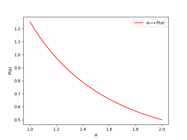
Figure 4: Graphical representation of the function $\alpha\longmapsto P_{\alpha}$. The leftmost value is $P_{1}=\sqrt{\frac{\pi}{2}}\simeq 1.2533$ and the right limit is $P_{2^{-}}=\frac{1}{2}$.

D.1 Precisions on the low noise-regime

In Section 5, we concluded the existence of two regimes predicted by our bounds. We first defined the low noise regime by the following condition:

$$\frac{\sigma_{1}\sqrt{d}}{R}<1.$$

However, the pre-factor $\alpha\longmapsto P_{\alpha}$ is decreasing. Therefore, we need to take it into account to accurately describe the regime where the generalization error is increasing with $\alpha$. This happens when we have:

$$\frac{P_{1}R}{\sigma_{1}\sqrt{d}}<\frac{P_{2}R^{2}}{d\sigma_{1}^{2}}.$$

Using Lemma 55, we get the condition that was mentioned briefly in Section 5:

$$\frac{\sigma_{1}\sqrt{d}}{R}<\frac{1}{\sqrt{2\pi}}.$$

D.2 Comparison with the constants appearing in other works

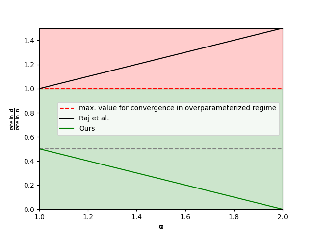
Figure 5: Comparison of the dimension dependence of our bounds and that of Raj et al. (2023b), under the assumption that $\ell$ is Lipschitz continuous, for both bounds.

In(Raj et al., 2023b), the authors prove expected generalization bounds for heavy-tail dynamics. The constant appearing in their bounds has a complex dependence on various constants defined in their assumptions, but we can sum up the dependence in $\alpha$ and $d$ as follows (by Applying Euler’s reflection formula to their Lemma $7$):

$$R_{\alpha,d}=\mathcal{O}\left(1+\frac{\sqrt{d}\Gamma\left(\frac{\alpha+d}{2}\right)}{(2-\alpha)\Gamma\left(1-\frac{\alpha}{2}\right)\Gamma\left(\frac{d}{2}\right)}\right)$$

By the proof of Lemma 12 and 13, we see that:

$$R_{\alpha,d}=\mathcal{O}\left(d^{\frac{1+\alpha}{2}}\right).$$

It is to be noted that our bound has a rate in $n$ of $1/2$, i.e. our bound is proportional to $1/\sqrt{n}$, while the bound of Raj et al. (2023b) has a rate of $1$, i.e. the bound is proportional to $1/n$. If we denote by $\Xi$ the ratio of the rate in $d$ to the rate in $n$ of the bound, we find (under a Lipschitz assumption for both bounds):

$$\Xi^{\text{(Ours)}}=1-\frac{\alpha}{2},\quad\Xi^{\text{\cite[citep]{(\@@bibref{AuthorsPhrase1Year}{raj_algorithmic_2023}{\@@citephrase{, }}{})}}}=\frac{1+\alpha}{2}.$$ (41)

The meaning of the coefficient $\Xi$ is that, in an overparameterized regime where $d>n$, the bound is non-vacuous only if $\Xi<1$. We graphically represented this coefficient in Figure 5.

Appendix E Discussion of the time dependence of the bounds

While Theorem 10 is the first high probability generalization bound for heavy-tailed dynamics, one may notice the time dependence of the bound, coming from the integral term, i.e.

$$\int_{0}^{T}\mathds{E}_{U}\left[\widehat{F}_{S}(W_{t})\right]dt.$$ (42)

Because of this term, as explained in Section 5, the light-tail limit of this bound leads to an informal bound of the form:

$$G_{S}(W_{t})\underset{\alpha\to 2^{-}}{\lesssim}\sqrt{\frac{1}{n\sigma^{2}}\int_{0}^{T}\mathds{E}_{U}\left[\widehat{F}_{S}(W_{t})\right]dt},$$

which is worse than the existing bounds on Langevin dynamics Mou et al. (2017); Li et al. (2020); Farghly and Rebeschini (2021), which achieve time-independent bounds. More explicitly, Mou et al. (2017) obtained a similar bound, but with an additional exponential time-decay in the integral term, i.e., informally,

$$\int_{0}^{T}e^{-a(T-t)}\mathds{E}_{U}\left[\widehat{F}_{S}(W_{t})\right]dt,$$

where $a>0$ is a constant dependent of the problem.

To the best of our knowledge, there is no obvious theoretical argument affirming that the limit $\alpha\to 2^{-}$ should exactly recover the bounds for Langevin dynamics, while it is quite clear that this limit should not be infinite, as in Raj et al. (2023b). That being said, it is worth discussing why this time dependence happens in our bound, how it could be improved, and, most importantly, why a time independent bound is currently beyond the reach of the theory.

Section 4.3 presents one step in the direction of time-uniform bounds. However, the integral term appearing in Theorem 11 is not satisfactory, because of its lack of interpretability, compared to Equation 42.

On the other hand, a more detailed analysis of the results of Mou et al. (2017); Li et al. (2020) shows that time-independence is a direct consequence of the use of a logarithmic Sobolev inequality (LSI, see Section A.3). If we translate these arguments in our setting, such an inequality would need to be satisfied by the prior distribution $\pi$. Therefore, it is natural to ask, whether we could apply Theorem 29 in our proofs.

A similar computation has been proposed by Gentil and Imbert (2008), in their study of the rate of convergence to equilibrium of an equation of the form of Equation 6. However, we argue that we cannot apply this reasoning in our setting. Let’s explain it briefly: in the proof of Theorem 10, the crucial term that appears in the computation of the entropy flow is what we called the Bregman integral, it is given by:

$$B_{\Phi}^{\alpha}(v)=C_{\alpha,d}\iint D_{\Phi}(v(x),v(x+z))\bar{u}_{\infty}d\nu_{\alpha}(z)dx.$$

On the other hand, Theorem 29 uses the following term, if we apply it to $\pi$ (in a similar way to how it is done in Section C.8.1):

$$\iint D_{\Phi}(v(x+z),v(x))\bar{u}_{\infty}d\nu_{\alpha}(z)dx.$$

Unfortunately, the Bregman divergence is not commutative in general, and, to the best of our knowledge, there is no obvious way of linking the two integrals appearing above. This discussion is the motivation behind Section 4.3, where we applied Theorem 29 and Lemma 7 to the case where the Bregman divergence becomes symmetric, i.e. when $\Phi(x)\propto x^{2}$.

Therefore, we conclude that we do not have the LSI that we would need to make our bounds time-independent. Let’s end this short discussion by writing down the result that we would obtain with such an inequality.

Theorem 56

We consider the same setting than in Theorem 10, but we additionally assume that the prior $\pi$ satisfies the following LSI, with reversed Bregman divergence compared to Theorem 29, for all $v$ smooth enough:

$$\text{Ent}_{\bar{u}_{\infty}}^{\Phi}\left(v\right)\leq\frac{C_{\alpha,d}\sigma_{1}^{\alpha}}{\alpha\eta}\iint D_{\Phi}(v(x),v(x+z))\bar{u}_{\infty}(x)d\nu_{\alpha}(z)dx.$$

Then, with probability at least $1-\zeta$ over $\mu_{z}^{\otimes n}$, we have:

$$\mathds{E}_{U}\left[G_{S}(W_{T}^{S})\right]\leq\sqrt{\frac{2K_{\alpha,d}}{\sigma_{1}^{\alpha}}\int_{0}^{T}e^{-\frac{\alpha\eta}{2}(T-t)}\mathds{E}_{U}\left[\left\|\nabla\widehat{F}_{S}(W^{S}_{t})\right\|^{2}\right]dt+\frac{\Lambda+\log(3/\zeta)}{n}}$$

with $\Lambda=\text{{{KL}}}\left(\rho_{0}||\bar{u}_{\infty}\right)$ and:

$$K_{\alpha,d}=\frac{(2-\alpha)\Gamma\left(1-\frac{\alpha}{2}\right)d\Gamma\left(\frac{d}{2}\right)}{\alpha 2^{\alpha}\Gamma\left(\frac{d+\alpha}{2}\right)R^{2-\alpha}},$$ (43)

Appendix F Additional experimental details

F.1 Hyperparameters details

In this section, we give a list of the exact hyperparameters used to obtain our main experiments. In general, those hyperparameters were chosen to make our experimental setting as close as possible to our theoretical setting and assumptions.

Linear model trained on MNIST (Figures 8 and 9) : We use a linear predictor, without bias, trained with a (multivariate cross-entropy loss). All $10$ classes of the MNIST dataset were used but we randomly subsample $10\%$ of the training set, to lower the computational cost of the experiments. We simulate Equation 16 with $T=5.10^{3}$, $\gamma=10^{-2}$, $\eta=10^{-3}$. The last $2000$ iterations were used to estimate the accuracy error, as described in Section F.2. During those experiments, we let $\alpha$ vary in $[1.6,2]$, using a linear scale of $10$ values. The parameter $\sigma$ varies in a logarithmic scale of $10$ values, such that $\sigma\sqrt{d}\in[0.5,40]$, where $d$ is the number of parameters in the model, this is inspired by the analysis of Section 5. This range was chosen to ensure both that the training is stable enough and that the heavy tail of the noise has an impact on the accuracy (i.e. $\sigma$ not too small).

$2$-layers FCN trained on MNIST: This experiment was used to produce Figures 1, 3 and 2. We use a $2$-layer neural network with ReLU activation, without bias, trained with a (multivariate cross-entropy loss). All $10$ classes of the MNIST dataset were used but we randomly subsample $10\%$ of the training set, to lower the computational cost of the experiments. We simulate Equation 16 with $T=10^{4}$, $\gamma=10^{-2}$, $\eta=10^{-3}$. The last $2000$ iterations were used to estimate the accuracy error, as described in Section F.2. During those experiments, we let $\alpha$ vary in $[1.6,2]$, using a linear scale of $10$ values. The width of the network varies in a linear scale of $10$ values, between $40$ and $200$.

FashionMNIST experiments: The same model was also used on the FashionMNIST dataset (a $10\%$ subsample of it), to obtain Figures 11, 10(a) and 10(b).

$5$-layers FCN trained on MNIST: We use a $5$-layer neural network with ReLU activation, without bias, trained with a (multivariate cross-entropy loss). $100\%$ of the MNIST dataset were used. We experimented using a batch-size in this case, i.e. Equation 16 is replaced by:

$$\hat{W}^{S}_{k+1}=\hat{W}^{S}_{k}-\frac{\gamma}{b}\sum_{j=1}^{b}\nabla f(\hat{W}^{S}_{k},z_{i_{j}})-\eta\gamma\hat{W}^{S}_{k}+\gamma^{\frac{1}{\alpha}}\sigma_{1}L_{1}^{\alpha},$$ (44)

where $b\in\mathds{N}^{\star}$ is the batch size and $(i_{1},\dots,i_{b})$ are random indices drawn at each iteration. We simulate Equation 16 with $T=10^{5}$, $\gamma=10^{-2}$, $\eta=10^{-3}$. The last $100$ iterations were used to estimate the accuracy error, as described in Section F.2. We used batch sizes $b\in\left\{64,128,256,512\right\}$. During those experiments, we let $\alpha$ vary in $[1.7,2]$, using a linear scale of $10$ values. In order for the training to be stable enough for the experiment to converge, we noted that we had to use smaller values, those values were chosen on a logarithmic scale of $6$ values so that $\sigma\sqrt{d}\in[0.1,3]$. It is probable that only the low noise regime, of Section 5, is then observable. Note that, in this case, i.e. when using mini-batches, we estimated the gradient norms $\left\|\nabla\widehat{F}_{S}\right\|$ using the batch gradients, appearing in Equation 44, instead of the whole empirical risk $\widehat{F}_{S}$. This makes sense as one of the goals of using batches is to reduce the computational cost of the experiments.

F.2 Accuracy evolution and robust mean estimation

Figures 6 and 7 show the evolution of both the train and test accuracy, during the first $2000$ iterations of training, for models and datasets similar to the one used for our main experiments (but with less data to make it easier to visualize). We show these curves for different values of the tail index $\alpha$ and of the quantity $\sigma\sqrt{d}$, which we argue in Section 5 has a strong impact on the training dynamics.

This allows us to observe two phenomenons, first, at least in these two experiments, there seems to be a transition, around the value $\sigma\sqrt{d}=1$. Indeed, for $\sigma\sqrt{d}\lesssim 1$, we observe that the tail of the noise has little impact on the evolution of both accuracies and therefore on the generalization error. On the other hand, for higher values of $\sigma\sqrt{d}$, we see the impact of the tail index $\alpha$. Indeed, the heavier the tail (i.e. the smaller $\alpha$), the more jumps are observed on both accuracies, which necessarily have an impact on the observed generalization. This seems to follow our theory developed in Section 5.

More importantly, the presence of those jumps makes the estimation of the generalization error, $G_{S}(W_{T}^{S})$, extremely noisy. To avoid this issue, we use the following two techniques:

1. The generalization error is averaged among the $2000$ last iterations (recall that we use $N\geq 5000$ in all our experiments so that the model is close to converence when we estimate the generalization error).

2. As the random jumps introduce values of the generalization error that are completely random and often much higher than the values between the jumps, we avoid them to bias the estimation by removing the $15\%$ upper quantile of the generalization error, in the last $2000$ iterations, before computing the mean.

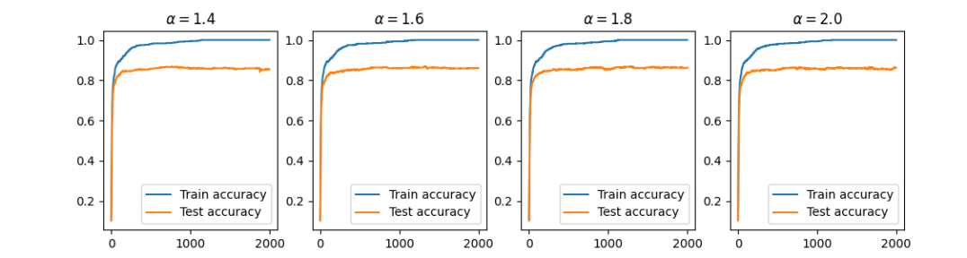
(a) $\sigma\sqrt{d}=0.1$

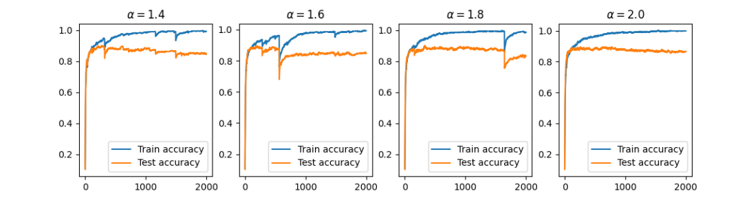
(b) $\sigma\sqrt{d}=1$

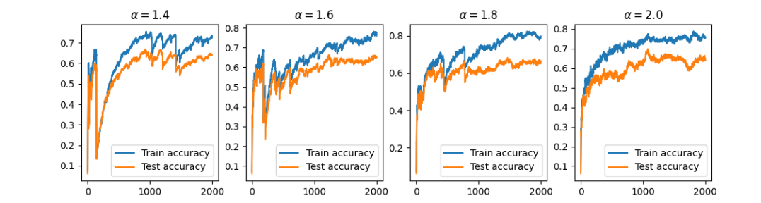
(c) $\sigma\sqrt{d}=10$

Figure 6: Evolution of the test and training accuracies, during the first $2000$ iterations, for the simulation of (3) with a linear model trained with a cross-entropy loss, on the MNIST dataset.

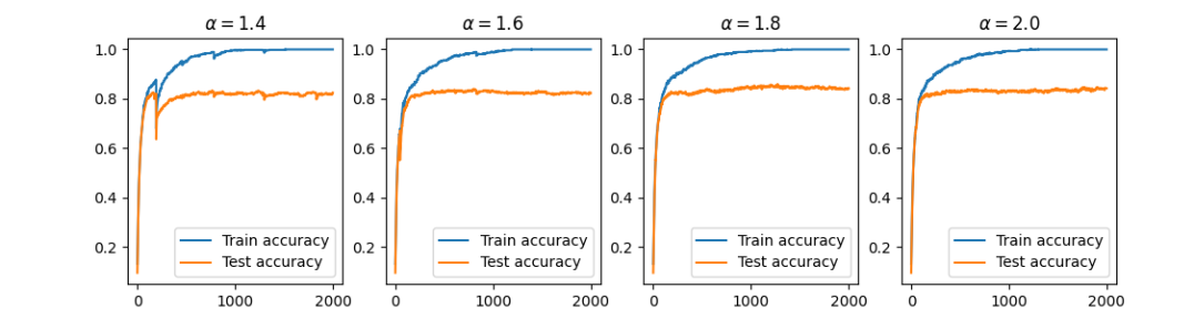
(a) $\sigma\sqrt{d}=1$

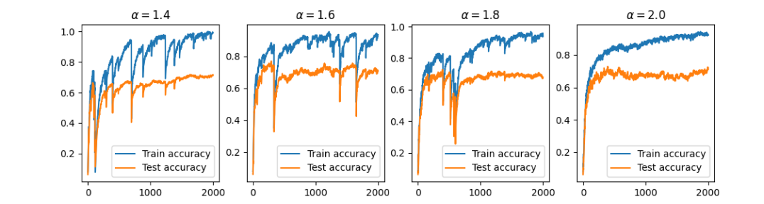
(b) $\sigma\sqrt{d}=10$

Figure 7: Evolution of the test and training accuracies, during the first $2000$ iterations, for the simulation of (3) with a $2$-layer neural network, trained with a cross-entropy loss, on the MNIST dataset.

F.3 Experimental procedures details

In this section, we quickly give more details on how the figures of Section 6 were obtained.

F.3.1 Bound estimation - Figures 2, 8 and 11

To get Figures 2, 8 and 11, we estimated the computable part of Equation 14. To do so, the gradient norm of all iterations where averaged, to get an estimate of the integral term:

$$\widehat{I}:=\gamma\sum_{k=1}^{N}\left\|\nabla\widehat{F}_{S}(\hat{W}_{k}^{S})\right\|^{2}\simeq\int_{0}^{T}\left\|\nabla\widehat{F}_{S}(W_{t}^{S})\right\|^{2}dt,$$ (45)

where $\gamma$ is the learning rate and $N$ the number of iterations. The quantity that is plotted on the $y$-axis of those figures is:

$$\widehat{G}:=\sqrt{\frac{P_{\alpha}d^{1-\frac{\alpha}{2}}}{n\sigma_{1}^{\alpha}R^{2-\alpha}}\widehat{I}}.$$ (46)

Moreover, this quantity is averaged over $10$ random seeds, with the same values of the hyperparameters $(\sigma,d,\alpha)$. Unless mentioned otherwise, the constant $R$, which is unknown a priori, is taken to be $R=1$ in the figures.

F.3.2 Correlation experiments - Figures 1 and 10(b)

Figures 1 and 10(b): In this experiment, we train a $2$-layers neural network on MNIST. The tail-index $\alpha$ varies in $[1.6,2]$ and the width of the network in $[40,200]$. To obtain the green curve, we proceed as follows:

• For each value fixed $w$ of the width, we compute Kendall’s correlation coefficient, denoted $\tau$, between the accuracy error and the tail-index $\alpha$.

• This gives us the correlation in terms of the width, i.e. a map $\tau(w)$.

• We repeat this procedure for $10$ random seeds.

• The green curve represents the mean value and standard deviation of $\tau(w)$.

For the dot black curve, to get a less noisy coefficient, we directly used, for each width $w$, the average of the accuracy error across all the random seeds, and we computed the correlation between $\alpha$ and this mean accuracy error. This is why there are no error bars in that case.

F.4 Additional experiments

In this subsection, we present a few additional experiments to further support the findings of Section 6. These additional experiments are organized as follows:

1. Additional experiments conducted on the FashionMNIST dataset (the experiments presented in Section 6 were all conducted on the MNIST dataset).

2. Additional experiments using a linear model.

3. More details figures regarding the use of mini-batches.

4. Interesting investigations regarding the value of the parameter $R$ appearing in Equation 14.

F.4.1 Additional experiment with linear models

We conducted experiments similar to that presented in Section 6 with a linear model, instead of a $2$-layers FCN. The results are presented in Figures 8 and 9. More specifically, in these experiments, we let both the noise scale $\sigma_{1}$ and the tail-index $\alpha$ vary in a fixed grid of values (see Section F.1). Note that, in this case, it is not possible to let the number of parameters vary without affecting the data, but we can act on $\sigma_{1}$ instead, and still test our theory. That being said, this model has the advantage, when using the cross-entropy as a surrogate loss, to fit nicely in our theoretical setting.

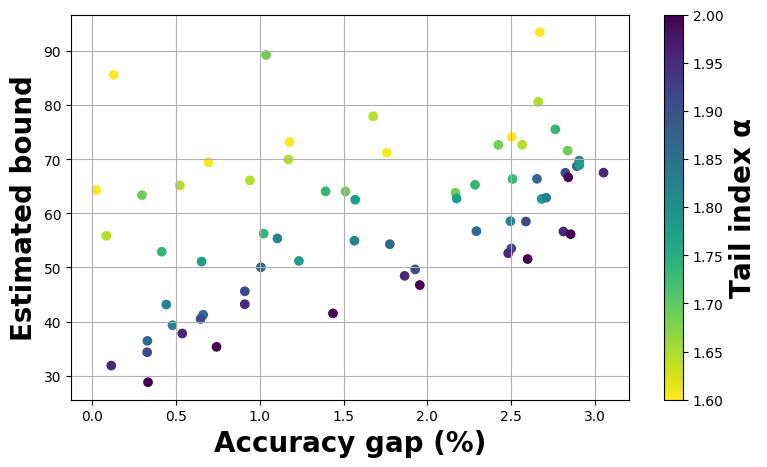
(a) $R=1$

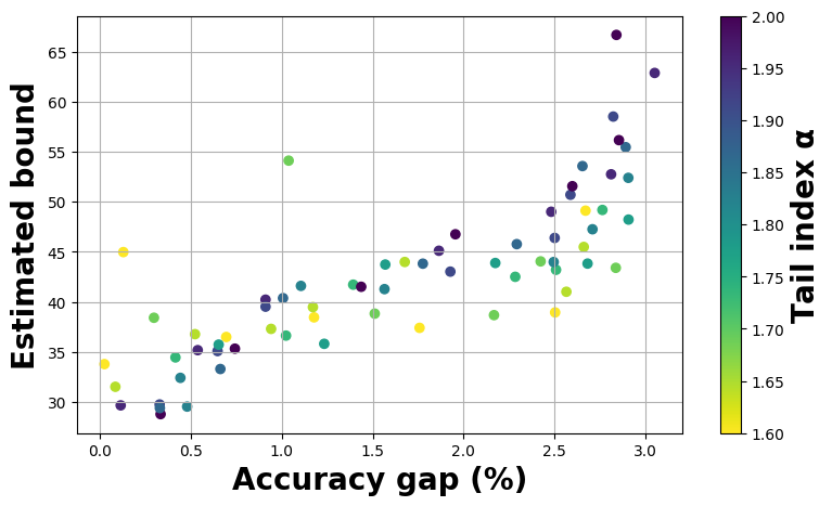
(b) $R=25$

Figure 8: Linear model on MNIST

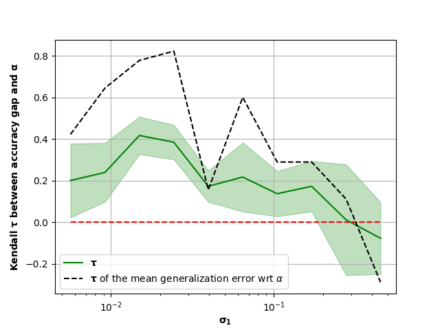
Figure 9: Correlation (Kendall’s $\tau$) between the tail index $\alpha$ and the accuracy gap for different values of the noise scale $\sigma_{1}$.

More specifically, we can see on Figure 8 that the estimated bound, according to Equation 46, correlates very well with the generalization error. On Figure 9, we show how the correlation between $\alpha$ and the accuracy gap varies when $\sigma_{1}$ is varying, see Section F.3. The phase transition, predicted in Section 5 is visible in this figure. An additional interesting phenomenon is observed on Figure 9. Indeed, on the left of the correlation plots (both the black and green curves), we can see that the Kendall’s $\tau$ coefficient, measuring the correlation between $\alpha$ and $G_{S}$, decreases. We interpret this as a third regime, when $\sigma_{1}$ is too small for our theory to hold and the algorithm starts behaving more like a deterministic gradient flow.

As we did on previous experiments, we can use Figure 9 and the analysis of Section 5 to estimate the value that the parameter $R$ takes in those experiments. Given that $d=7840$ in this experiment and that the phase transition seems to be happening around $\sigma_{1}\simeq 0.3$, we can estimate $R\simeq\sigma_{1}\sqrt{d}\simeq 26$. On Figure 8, we plotted the estimated bound both for $R=1$ (our default choice) along with the estimated bound for $R=25$. We observe on that second figure a much improved correlation, hence supporting the experimental results of Section 6.

Remark 57

With this linear model experiment, it is not possible to let the number of parameters vary (at least not without affecting the data), it is therefore not possible to test the dimension dependence, as in Figure 3, in this case.

F.4.2 Additional experiments on the FashionMNIST dataset

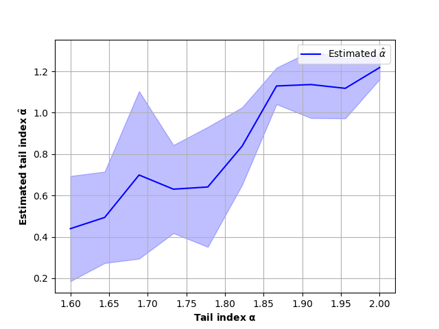
(a) Regression of the parameter $\alpha$ from the accuracy error, for a $2$-layers network trained on $10\%$ of the FashionMNIST dataset.

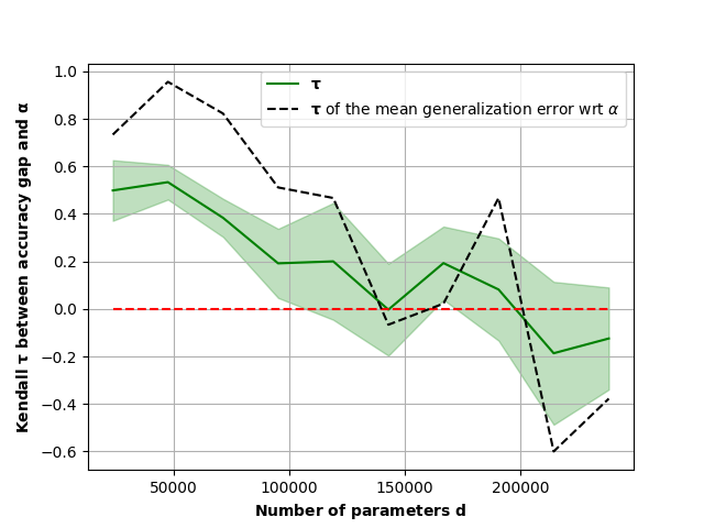
(b) Correlation between $\alpha$ and the accuracy error, for a $2$-layers network trained on $10\%$ of the FashionMNIST dataset, with varying width.

Figure 10: Experiments with a $2$-layers FCN and the FshionMNIST dataset.

We conducted the same experiments as those presented on Figures 3 and 1 on the Fashion MNIST dataset. The results are presented in Figures 10(a) and 10(b). We observe the exact same behavior than the experiments conducted on the MNIST dataset: the regression of the tail index shows a remarkable correlation with the ground truth $\alpha$, with the expected monotonicity, even though the value of $\alpha$ is underestimated. Moreover, the phase transition, between the two regimes predicted in Section 5, is observable in Figure 10(b). It seems to happen at a higher value of $d$ than in the MNIST experiment.

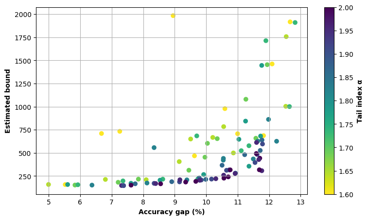
(a) $R=4$

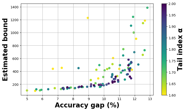
(b) $R=11$

Figure 11: FasionMNIST

Additionally, we present in Figure 11 the value of the estimated bound, based on Equation 46, compared to the accuracy gap, for different values of th parameter $R$. For the default choice $R=1$, we already observe a very good correlation. Based on Figure 10(b), using the same procedure than in our previous experiments, we can estimate the value of $R$ to be about $R\simeq 11$. As we observe in all our previous experiments, in Sections 6 and F.4.1, we observe that taking into account this value of $R$ improves the observed correlation betzeen the bound and the accuracy gap, hence supporting the theory.

F.4.3 Additional experiments with the full MNIST dataset and mini-batches

As already mentioned in Section 6, in order to argue that our bounds may also be pertinent in more practical settings than the figure presented in the rest of the paper, we computed our bound using a FCN$5$, on the full MNIST dataset, using mini-batches. This is to be compared eith our other experiments, were, according to the SDE we study, we take the full batch at each iteration to compute $\nabla\widehat{F}_{S}$. The exact procedure and hyperparameters are detailed, as for other experiments, in Section F.1. These results are shown on Figure 12, were we observe that, for several values of the batch size, we still observe a very good correlation between the estimated bound and the generalization error. Unfortunately, our theroy does not predict the behavior of the accuracy gap with respect to the batch-size, but, from this experiment, we understand that it is still capturing relatively well the behavior of the accuracy gap.

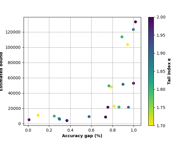
(a) Batch size $64$

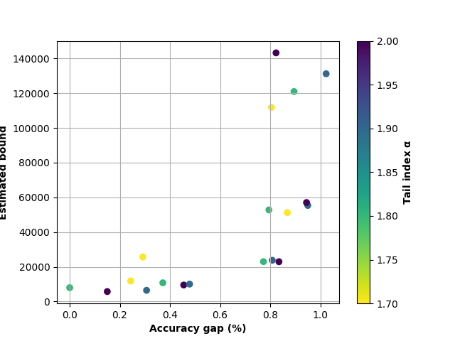
(b) Batch size $128$

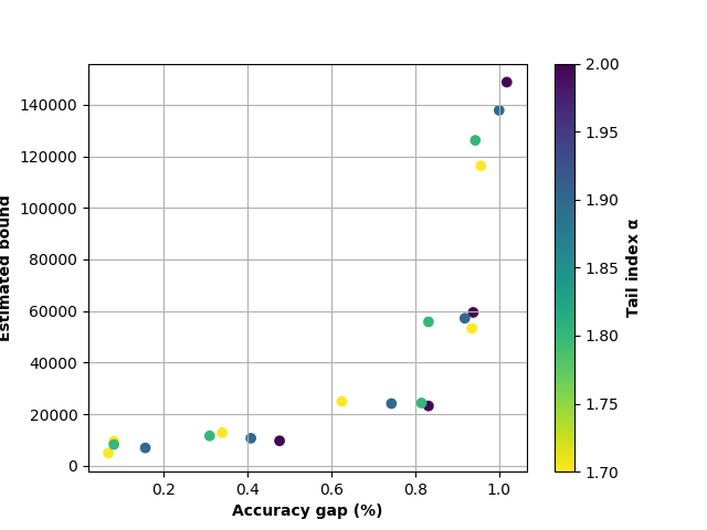
(c) Batch size $256$

Figure 12: Estimated bound, computed with Equation 46, versus accuracy gap, for a $5$-layers FCN on the full MNIST dataset, for different value of batch size.

References

- Alquier (2021) Pierre Alquier. User-friendly introduction to PAC-Bayes bounds, November 2021.
- Bakry et al. (2014) Dominique Bakry, Ivan Gentil, and Michel Ledoux. Analysis and Geometry of Markov Diffusion Operators. Springer, 2014.
- Barsbey et al. (2021) Melih Barsbey, Milad Sefidgaran, Murat A. Erdogdu, Gaël Richard, and Umut Şimşekli. Heavy Tails in SGD and Compressibility of Overparametrized Neural Networks. In 35th Conference on Neural Information Processing Systems (NeurIPS 2021). arXiv, June 2021. doi: 10.48550/arXiv.2106.03795.
- Birdal et al. (2021) Tolga Birdal, Aaron Lou, Leonidas Guibas, and Umut Şimşekli. Intrinsic Dimension, Persistent Homology and Generalization in Neural Networks. Advances in Neural Information Processing Systems 34 (NeurIPS 2021), November 2021.
- Bogachev (2007) V. I. Bogachev. Measure theory. Vol. I, II. Springer-Verlag, Berlin, 2007. ISBN 978-3-540-34513-8; 3-540-34513-2. doi: 10.1007/978-3-540-34514-5.
- Böttcher et al. (2013) Björn Böttcher, René Schilling, and Jian Wang. Lévy Matters III: Lévy-Type Processes: Construction, Approximation and Sample Path Properties, volume 2099 of Lecture Notes in Mathematics. Springer International Publishing, Cham, 2013. ISBN 978-3-319-02683-1 978-3-319-02684-8. doi: 10.1007/978-3-319-02684-8.
- Bousquet (2002) Olivier Bousquet. Stability and generalization. Journal of Machine Learning Research, pages 499–526, 2002.
- Bousquet et al. (2020) Olivier Bousquet, Yegor Klochkov, and Nikita Zhivotovskiy. Sharper bounds for uniformly stable algorithms. Proceedings of Thirty Third Conference on Learning Theory, May 2020.
- Catoni (2007) Olivier Catoni. Pac-Bayesian Supervised Classification: The Thermodynamics of Statistical Learning. IMS Lecture Notes Monograph Series, 56:1–163, 2007. ISSN 0749-2170. doi: 10.1214/074921707000000391.
- Chafai (2004) Djalil Chafai. Entropies, convexity, and functional inequalities. Kyoto Journal of Mathematics, 44(2), January 2004. ISSN 2156-2261. doi: 10.1215/kjm/1250283556.
- Chafai and Lehec (2017) Djalil Chafai and Joseph Lehec. Logarithmic sobolev inequalities essentials. 2017.
- Dalalyan (2016) Arnak S. Dalalyan. Theoretical guarantees for approximate sampling from smooth and log-concave densities, December 2016.
- (13) Maha Daoud and El Haj Laamri. Fractional Laplacians : A short survey. Discrete and Continuous Dynamical Systems.
- Duan (2015) Jinqiao Duan. An Introduction to Stochastic Dynamics. Cambridge texts in Applied Mathematics, 2015.
- Dupuis et al. (2023) Benjamin Dupuis, George Deligiannidis, and Umut Şimşekli. Generalization Bounds with Data-dependent Fractal Dimensions. In Internation Conference on Machine Learning (ICML 2023). arXiv, February 2023. doi: 10.48550/arXiv.2302.02766.
- Farghly and Rebeschini (2021) Tyler Farghly and Patrick Rebeschini. Time-independent Generalization Bounds for SGLD in Non-convex Settings. In 35th Conference on Neural Information Processing Systems (NeurIPS 2021). arXiv, November 2021. doi: 10.48550/arXiv.2111.12876.
- Favaro et al. (2020) Stefano Favaro, Sandra Fortini, and Stefano Peluchetti. Stable behaviour of infinitely wide deep neural networks. In Proceedings of the 23rdInternational Conference on Artifi- Cial Intelligence and Statistics (AISTATS) 2020. arXiv, February 2020.
- Futami and Fujisawa (2023) Futoshi Futami and Masahiro Fujisawa. Time-Independent Information-Theoretic Generalization Bounds for SGLD. In 7th Conference on Neural Information Processing Systems (NeurIPS 2023). arXiv, November 2023. doi: 10.48550/arXiv.2311.01046.
- Gentil and Imbert (2008) Ivan Gentil and Cyril Imbert. Logarithmic Sobolev inequalities: Regularizing effect of Lévy operators and asymptotic convergence in the Lévy-Fokker-Planck equation. Asymptotic analysis, September 2008.
- Germain et al. (2009) Pascal Germain, Alexandre Lacasse, François Laviolette, and Mario Marchand. PAC-Bayesian learning of linear classifiers. In Proceedings of the 26th Annual International Conference on Machine Learning, ICML ’09, pages 353–360, New York, NY, USA, June 2009. Association for Computing Machinery. ISBN 978-1-60558-516-1. doi: 10.1145/1553374.1553419.
- Gross (1975) L. Gross. Logarithmic Sobolev inequalities. Amer. J. Math., 97(4):1061–1083, 1975.
- Gurbuzbalaban and Hu (2021) Mert Gurbuzbalaban and Yuanhan Hu. Fractional moment-preserving initialization schemes for training deep neural networks. In Proceedings of the 24th International Conference on Artifi- Cial Intelligence and Statistics (AISTATS) 2021. arXiv, February 2021.
- Gurbuzbalaban et al. (2021) Mert Gurbuzbalaban, Umut Şimşekli, and Lingjiong Zhu. The Heavy-Tail Phenomenon in SGD. In International Conference on Machine Learning (ICML 2021). arXiv, June 2021. doi: 10.48550/arXiv.2006.04740.
- Haghifam et al. (2020) Mahdi Haghifam, Jeffrey Negrea, Ashish Khisti, Daniel M. Roy, and Gintare Karolina Dziugaite. Sharpened Generalization Bounds based on Conditional Mutual Information and an Application to Noisy, Iterative Algorithms, October 2020.
- Halperin and Schwartz (1952) Israel Halperin and Laurent Schwartz. Introduction to the Theory of Distributions. University of Toronto Press, 1952. ISBN 978-1-4875-9132-8.
- Hodgkinson and Mahoney (2020) Liam Hodgkinson and Michael W. Mahoney. Multiplicative noise and heavy tails in stochastic optimization. In Proceedings of the 38 Th International Conference on Machine Learning (ICML 2021). arXiv, June 2020. doi: 10.48550/arXiv.2006.06293.
- Hodgkinson et al. (2022) Liam Hodgkinson, Umut Şimşekli, Rajiv Khanna, and Michael W. Mahoney. Generalization Bounds using Lower Tail Exponents in Stochastic Optimizers. Proceedings of the 39th International Conference on Machine Learning, July 2022.
- Imbert (2005) Cyril Imbert. A non-local regularization of first order Hamilton-Jacobi equations. Journal of differential equations, 2005.
- Jung et al. (2021) Paul Jung, Hoil Lee, Jiho Lee, and Hongseok Yang. $\alpha$-Stable convergence of heavy-tailed infinitely-wide neural networks. Advances in Applied Probability , Volume 55 , Issue 4, June 2021.
- Kendall (1938) Maurice G. Kendall. A new reasure of rank correlation. Biometrika, 1938.
- Kühn (2018) Franziska Kühn. Solutions of Lévy-driven SDEs with unbounded coefficients as Feller processes. Proceedings of the American Mathematical Society, 146(8):3591–3604, 2018.
- Lafleche (2020) Laurent Lafleche. Fractional Fokker-Planck Equation with General Confinement Force. SIAM Journal on Mathematical Analysis, 52(1):164–196, January 2020. ISSN 0036-1410, 1095-7154. doi: 10.1137/18M1188331.
- Lecun et al. (1998) Y. Lecun, L. Bottou, Y. Bengio, and P. Haffner. Gradient-based learning applied to document recognition. Proceedings of the IEEE, 86(11):2278–2324, November 1998. ISSN 1558-2256. doi: 10.1109/5.726791.
- Li et al. (2020) Jian Li, Xuanyuan Luo, and Mingda Qiao. On Generalization Error Bounds of Noisy Gradient Methods for Non-Convex Learning. In Published as a Conference Paper at ICLR 2020. arXiv, February 2020. doi: 10.48550/arXiv.1902.00621.
- Lim et al. (2022) Soon Hoe Lim, Yijun Wan, and Umut Şimşekli. Chaotic Regularization and Heavy-Tailed Limits for Deterministic Gradient Descent, May 2022.
- Lischke et al. (2019) Anna Lischke, Guofei Pang, Mamikon Gulian, Fangying Song, Christian Glusa, Xiaoning Zheng, Zhiping Mao, Wei Cai, Mark M. Meerschaert, Mark Ainsworth, and George Em Karniadakis. What Is the Fractional Laplacian? - A comparative review with new results, November 2019.
- Markowich and Villani (2004) P.A. Markowich and C. Villani. On the Trend to Equilibrium for the Fokker-Planck Equation: An Interplay between Physics and Functional Analysis. 2004.
- Maurer (2004) Andreas Maurer. A Note on the PAC Bayesian Theorem, November 2004.
- McAllester (1998) David McAllester. Some pac-bayesian theorems. In Proceedings of the Eleventh Annual Conference on Computational Learning Theory, COLT 1998, Madison, Wisconsin, USA, July 24-26, 1998, pages 230–234. ACM, 1998.
- McAllester (2003) David A. McAllester. PAC-Bayesian Stochastic Model Selection. Machine Learning, 51(1):5–21, April 2003. ISSN 1573-0565. doi: 10.1023/A:1021840411064.
- Mou et al. (2017) Wenlong Mou, Liwei Wang, Xiyu Zhai, and Kai Zheng. Generalization Bounds of SGLD for Non-convex Learning: Two Theoretical Viewpoints. In Proceedings of the 31st Conference On Learning Theory. arXiv, July 2017. doi: 10.48550/arXiv.1707.05947.
- Negrea et al. (2020) Jeffrey Negrea, Mahdi Haghifam, Gintare Karolina Dziugaite, Ashish Khisti, and Daniel M. Roy. Information-Theoretic Generalization Bounds for SGLD via Data-Dependent Estimates, January 2020.
- Neu et al. (2021) Gergely Neu, Gintare Karolina Dziugaite, Mahdi Haghifam, and Daniel M. Roy. Information-Theoretic Generalization Bounds for Stochastic Gradient Descent, August 2021.
- Nguyen et al. (2019a) Than Huy Nguyen, Umut Simsekli, and Gaël Richard. Non-asymptotic analysis of fractional langevin monte carlo for non-convex optimization. In International Conference on Machine Learning, pages 4810–4819. PMLR, 2019a.
- Nguyen et al. (2019b) Thanh Huy Nguyen, Umut Şimşekli, Mert Gürbüzbalaban, and Gaël Richard. First Exit Time Analysis of Stochastic Gradient Descent Under Heavy-Tailed Gradient Noise. In NIPS’19: Proceedings of the 33rd International Conference on Neural Information Processing Systems. arXiv, June 2019b. doi: 10.48550/arXiv.1906.09069.
- Pavasovic et al. (2023) Krunoslav Lehman Pavasovic, Alain Durmus, and Umut Simsekli. Approximate heavy tails in offline (multi-pass) stochastic gradient descent. In Advances in Neural Information Processing Systems, 2023.
- Pensia et al. (2018) Ankit Pensia, Varun Jog, and Po-Ling Loh. Generalization Error Bounds for Noisy, Iterative Algorithms. 2018 IEEE International Symposium on Information Theory (ISIT), January 2018.
- Raginsky et al. (2017) Maxim Raginsky, Alexander Rakhlin, and Matus Telgarsky. Non-convex learning via Stochastic Gradient Langevin Dynamics: A nonasymptotic analysis, June 2017.
- Raj et al. (2023a) Anant Raj, Melih Barsbey, Mert Gürbüzbalaban, Lingjiong Zhu, and Umut Şimşekli. Algorithmic Stability of Heavy-Tailed Stochastic Gradient Descent on Least Squares. In Proceedings of The 34th International Conference on Algorithmic Learning Theory,. arXiv, February 2023a. doi: 10.48550/arXiv.2206.01274.
- Raj et al. (2023b) Anant Raj, Lingjiong Zhu, Mert Gürbüzbalaban, and Umut Şimşekli. Algorithmic Stability of Heavy-Tailed SGD with General Loss Functions. In International Conference on Machine Learning (ICML 2023). arXiv, January 2023b. doi: 10.48550/arXiv.2301.11885.
- Schertzer et al. (2001) D. Schertzer, M. Larchev, J. Duan, V. V. Yanovsky, and S. Lovejoy. Fractional Fokker–Planck Equation for Nonlinear Stochastic Differential Equations Driven by Non-Gaussian Levy Stable Noises. Journal of Mathematical Physics, 42(1):200–212, January 2001. ISSN 0022-2488, 1089-7658. doi: 10.1063/1.1318734.
- Schilling (1998) René L. Schilling. Feller Processes Generated by Pseudo-Differential Operators: On the Hausdorff Dimension of Their Sample Paths — SpringerLink. Journal of Theoretical Probability, 1998.
- Schilling (2016) René L. Schilling. An Introduction to Lévy and Feller Processes. Advanced Courses in Mathematics - CRM Barcelona 2014, October 2016.
- Schilling and Schnurr (2010) Rene L. Schilling and Alexander Schnurr. The Symbol Associated with the Solution of a Stochastic Differential Equation. Electr. J. Probab. 15, December 2010.
- Shawe-Taylor and Williamson (1997) John Shawe-Taylor and Robert C. Williamson. A PAC analysis of a bayesian estimator. In Yoav Freund and Robert E. Schapire, editors, Proceedings of the Tenth Annual Conference on Computational Learning Theory, COLT 1997, Nashville, Tennessee, USA, July 6-9, 1997, pages 2–9. ACM, 1997.
- Şimşekli (2017) Umut Şimşekli. Fractional langevin monte carlo: Exploring lévy driven stochastic differential equations for markov chain monte carlo. In International Conference on Machine Learning, pages 3200–3209. PMLR, 2017.
- Simsekli et al. (2019) Umut Simsekli, Levent Sagun, and Mert Gurbuzbalaban. A Tail-Index Analysis of Stochastic Gradient Noise in Deep Neural Networks. In Proceedings of the 36 Th International Conference on Machine Learning (ICML 2019). arXiv, January 2019. doi: 10.48550/arXiv.1901.06053.
- Şimşekli et al. (2021) Umut Şimşekli, Ozan Sener, George Deligiannidis, and Murat A. Erdogdu. Hausdorff Dimension, Heavy Tails, and Generalization in Neural Networks. Journal of Statistical Mechanics: Theory and Experiment, 2021(12):124014, December 2021. ISSN 1742-5468. doi: 10.1088/1742-5468/ac3ae7.
- Teymurazyan (2023) Rafayel Teymurazyan. The fractional Laplacian: A primer. https://arxiv.org/abs/2310.19118v1, October 2023.
- Tristani (2013) Isabelle Tristani. Fractional Fokker-Planck equation. Commun. Math. Sci. 13, December 2013.
- Umarov et al. (2018) Sabir Umarov, Marjorie Hahn, and Kei Kobayashi. Beyond the Triangle: Brownian Motion, Ito Calculus and Fokker-Planck Equation - Fractional Generalizations. World scientific publishing, 2018.
- van Erven and Harremoës (2014) Tim van Erven and Peter Harremoës. Rényi Divergence and Kullback-Leibler Divergence. IEEE Transactions on Information Theory, 60(7):3797–3820, July 2014. ISSN 0018-9448, 1557-9654. doi: 10.1109/TIT.2014.2320500.
- Vershynin (2020) Roman Vershynin. High-Dimensional Probability - An Introduction with Application in Data Science. University of California - Irvine, 2020.
- Viallard et al. (2021) Paul Viallard, Pascal Germain, Amaury Habrard, and Emilie Morvant. A General Framework for the Disintegration of PAC-Bayesian Bounds. Machine Learning Journal, October 2021.
- Villani (2009) Cédric Villani. Optimal Transport - Old and New. Springer, 2009.
- Wan et al. (2023) Yijun Wan, Abdellatif Zaidi, and Umut Simsekli. Implicit compressibility of overparametrized neural networks trained with heavy-tailed sgd. arXiv preprint arXiv:2306.08125, 2023.
- Wang and Duan (2017) Ming Wang and Jinqiao Duan. Existence and regularity of a linear nonlocal Fokker–Planck equation with growing drift. Journal of Mathematical Analysis and Applications, 449(1):228–243, May 2017. ISSN 0022-247X. doi: 10.1016/j.jmaa.2016.12.013.
- Wu (2000) Liming Wu. A new modified logarithmic Sobolev inequality for Poisson point processes and several applications. Probability theory and related fileds - s 118, 427–438, 2000.
- Xiao et al. (2017) Han Xiao, Kashif Rasul, and Roland Vollgraf. Fashion-MNIST: A Novel Image Dataset for Benchmarking Machine Learning Algorithms, September 2017.
- Xiao (2004) Yimin Xiao. Random fractals and Markov processes. Fractal Geometry and Applications: A jubilee of Benoît Mandelbrot - American Mathematical Society, 72.2:261–338, 2004. doi: 10.1090/pspum/072.2/2112126.
- Xie et al. (2015) Xiaoxia Xie, Jinqiao Duan, Xiaofan Li, and Guangying Lv. A regularity result for the nonlocal Fokker-Planck equation with Ornstein-Uhlenbeck drift, April 2015.
- Zhou et al. (2020) Pan Zhou, Jiashi Feng, Chao Ma, Caiming Xiong, Steven Chu Hong Hoi, et al. Towards theoretically understanding why sgd generalizes better than adam in deep learning. Advances in Neural Information Processing Systems, 33:21285–21296, 2020.