Assembly bias in eBOSS

Abstract

Context. Analytical models of galaxy-halo connection such as the Halo Occupation Distribution (HOD) model have been widely used over the past decades as a means to intensively test perturbative models on quasi-linear scales. However, these models fail to reproduce the galaxy-galaxy lensing signal on non-linear scales, over-predicting the observed signal up to $40\%$.

Aims. With ongoing Stage-IV galaxy surveys such as DESI and EUCLID, it is now crucial to accurately model the galaxy-halo connection up to intra-halo scales to accurately estimate theoretical uncertainties of perturbative models.

Methods. This paper compares the standard HOD model (based on halo mass only) to an extended HOD framework that incorporates as additional features galaxy assembly bias and local environmental dependencies on halo occupation. These models have been calibrated against the observed clustering and galaxy-galaxy lensing signal of eBOSS Luminous Red Galaxies (LRG) and Emission Lines Galaxies (ELG) in the range $0.6<z<1.1$. A combined clustering-lensing cosmological analysis is then performed on the simulated galaxy samples of both standard and extended HOD frameworks to quantify the systematic budget of perturbative models.

Results. By considering not only the mass of the dark matter halos but also these secondary properties, the extended HOD model offers a more comprehensive understanding of the connection between galaxies and their surroundings. In particular, we found that the LRGs preferentially occupy denser and more anisotropic environments. Our results highlight the importance of considering environmental factors in galaxy formation models, with an extended HOD framework that reproduces the observed signal within $20\%$ on scales below 10 $h^{-1}$Mpc. Our cosmological analysis reveals that our perturbative model yields similar constraints regardless of the galaxy population, with a better goodness of fit for the extended HOD. These results suggest that the extended HOD framework should be used to quantify modeling systematics. This extended framework should also prove useful for forward modeling techniques.

1 Introduction

In the standard model of cosmology, galaxies are predicted to form and evolve within dark matter halos. To extract cosmological information from observed galaxy clustering, it is mandatory to understand galaxy formation and thus the connection between galaxies and their host dark matter halos beyond their linear relationship on large scales (Kaiser, 1984). One of the most popular and efficient models of the galaxy-halo connection for large-scale cosmological studies is the Halo Occupation Distribution model (HOD, Berlind & Weinberg (2002); Zheng et al. (2005, 2007)). In the standard HOD framework, it is assumed that all galaxies live inside dark matter halos and that galaxy occupation, which corresponds to the probability for a halo of hosting a galaxy, is solely determined by halo mass. This assumption has emerged as halo mass is the halo property that most strongly correlates with halo abundances and clustering as well as galaxy intrinsic properties (White & Rees, 1978). However, a large number of studies has shown that the mass-only HOD does not properly model galaxy clustering on small scales (below $10h^{-1}$Mpc), and that halo occupation depends on secondary halo properties beyond halo mass. (Artale et al., 2018; Zehavi et al., 2018; Bose et al., 2019; Hadzhiyska et al., 2020, 2023a, 2023b). In particular, it has been shown that galaxy occupation is correlated with halo formation time, a phenomenon referred to as galaxy assembly bias,(Dalal et al., 2008) as well as environmental properties, such as local density and local anisotropies, as one can predict from first principles for instance using excursion-set theory (Musso et al., 2018). In the previous study of Yuan et al. (2021, 2022), it has been shown that the standard framework fails to model accurately the full two-dimensional redshift space clustering of the Sloan Digital Sky Survey BOSS CMASS sample (Dawson et al., 2013), and that an extended HOD framework which incorporates assembly bias and environmental dependence of halo occupation agrees better with the data. In particular, the observed discrepancy of $30-40\%$ between the observed galaxy-galaxy lensing (GGL) signal of CMASS galaxies and the standard HOD framework (Leauthaud et al., 2017), a tension referred to as ’lensing is low’, can be partially resolved with the extended model (Contreras et al., 2023) so as to account for the impact of galaxy physics (Gouin et al., 2019; Chaves-Montero et al., 2023). However, no study has shown if these small scales discrepancy might bias or not the extraction of cosmological information. Here, we investigate this matter with the galaxies observed with the extended BOSS survey (Dawson et al., 2016), by directly fitting the GGL signal from the standard and extended HOD framework.
The paper is organized as follows: In Section 2, we briefly present the observations. In Section 3, we describe the implementation of the standard and extended HOD framework as well as our fitting procedure. Finally, we present the results of our analysis in Section 4 and conclude in Section  5. We also provide additional information in the Appendix A and B.

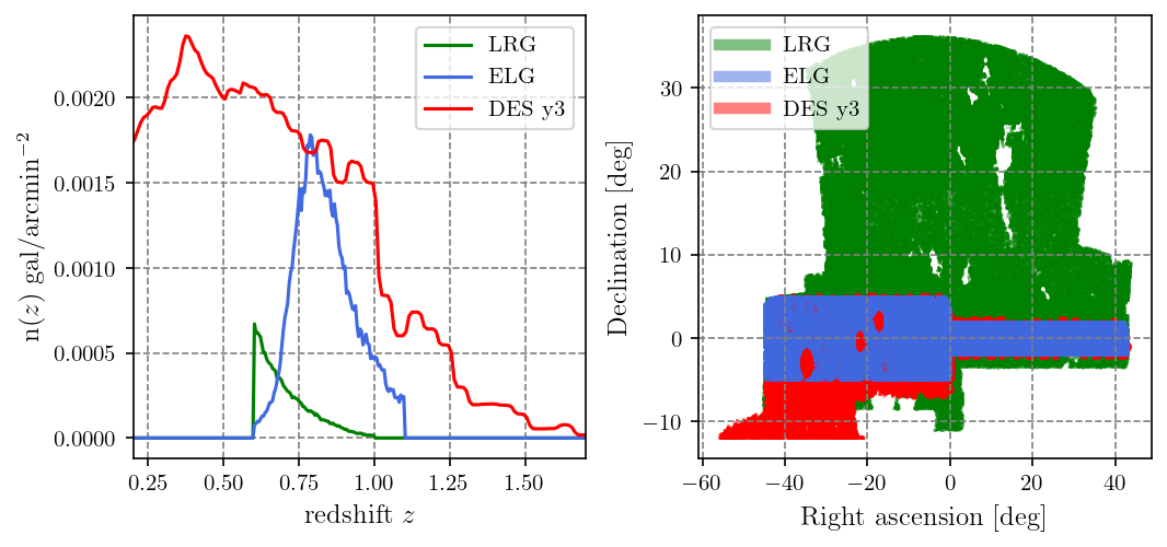
Figure 1: Galaxy number density (left panel) and footprint (right panel) of the LRG sample (green), the ELG sample (blue), and the DES y3 GOLD catalog (red). The n(z) of DES corresponds to the concatenation of the n(z) on each tomographic bin (Myles et al., 2021). It has been sub-sampled by a factor 20 for clarity. On the right panel, we present the DES footprint with a cut below a declination of - 12.

2 Data

2.1 eBOSS and DES catalogs

The extended Baryon Oscillation Spectroscopic Survey (eBOSS; Dawson et al. (2016)) measured thousands of spectra of galaxies and quasars in the range $0.6<z<2.4$ in order to probe the geometry and growth rate of the Universe over cosmic time. In this work, we study the properties of the Emission Line Galaxies (ELGs) and eBOSS Luminous Red Galaxies (LRGs) combined with the BOSS CMASS sample. Description of these samples can be found in Ross et al. (2020) and their cosmological analyses in Tamone et al. (2020); de Mattia et al. (2021); Bautista et al. (2021); Gil-Marín et al. (2020). We focus our attention on the South Galactic Cap (SGC), where 121 717 LRGs and 89 967 ELGs were observed in the range $0.6<z<1.0$ and $0.6<z<1.1$. In addition to the clustering properties of these galaxies, we aim to extract information from the GGL signal. This is achieved with the shape measurements of the Dark Energy Survey (DES) Year 3(Dark Energy Survey Collaboration et al., 2016). We used the main Y3 DES catalog (referred as ’Gold’) ; Information of the photometry and shape measurements of this sample can be found in Sevilla-Noarbe et al. (2021); Gatti et al. (2021) and the corresponding cosmological 3x2pt analysis is presented in Abbott et al. (2022). The radial distribution and the footprint of each survey are presented in Fig 1. eBOSS and DES overlap in a small portion, around 754 deg², of the SGC. In the overlapping area, 14 413 244 sources can be used to infer the GGL signal of 44 456 LRG lenses, while all of the observed ELGs are within the DES footprint.

2.2 The UCHUU simulation

In order to model the observed signals, we relied on the N-Body simulation uchuu (Ishiyama et al., 2021). This simulation was run with GreeM, a massively parallel TreePM code (Ishiyama et al., 2009, 2012), with initial conditions produced by second-order Lagrangian perturbation theory starting at a redshift $z=127$. The cosmological flat $\Lambda$CDM parameters of the simulation are compatible with the ones measured by Planck Collaboration et al. (2016), ($\Omega_{\mathrm{m}},\Omega_{\mathrm{b}},h,n_{s},\sigma_{8})=(0.3089,0.0486,0.6774,0.9667,0.8159)$. uchuu is one of the most precise N-Body simulations to date, with 12 800³ dark matter particles with mass $3.27\times 10^{8}h^{-1}$ $M_{\odot}$ in a box of side-length $L=2h^{-1}$Gpc. This large volume enables us to study a large number of dark matter halos up to a very high mass of $M\approx 10^{14.8}h^{-1}$ $M_{\odot}$. These halos were identified with the RockStar halo finder (Behroozi et al., 2013). We extracted from the simulation the halo and sub-halo catalogs of mass $M>10^{11}h^{-1}$ M_⊙ and the particle distribution (sub-sampled by a factor 0.005), at redshifts $z=0.86$ and $z=0.7$, corresponding to the effective redshift of the ELG and LRG samples respectively.

3 Halo Occupation model

3.1 Standard HOD parametrisation

In order to simulate realistic galaxy distributions from the uchuu simulation, we populate halos using the standard halo occupation distribution (HOD) description. For LRG, we consider the HOD framework first described in Zheng et al. (2005, 2007) and widely used in previous BOSS and eBOSS studies (White et al., 2011; Zhai et al., 2017). For emission line galaxies, we use the Gaussian HOD model (GHOD) Avila et al. (2020); Rocher et al. (2023a) for central occupation. Hence, let us first define the mean central halo occupations as

$$\left\langle N_{\mathrm{cen}}^{\text{LRG}}(M)\right\rangle =\frac{f_{\text{ic}}}{2}\left[1+\operatorname{erf}\left(\frac{\log M-\log M_{\min}^{\text{LRG}}}{\sigma_{\mathrm{M},{\text{LRG}}}}\right)\right],$$ (1)

$$\left\langle N_{\mathrm{cen}}^{\text{ELG}}(M)\right\rangle =\frac{A_{c}}{\sqrt{2\pi}\sigma_{\mathrm{M},\text{ELG}}}\cdot\exp{-\frac{\left(\log M-\log M_{\min}^{\text{ELG}}\right)^{2}}{2\sigma_{\mathrm{M},\text{ELG}}^{2}}},$$ (2)

where the $M_{\mathrm{min}}$ are the halo mass for which half of the halos have a central galaxy, the $\sigma_{\mathrm{M}}$ correspond to the scatter of central occupations, and $f_{\text{ic}}$ and $A_{c}$ correspond to completeness factors . The satellite occupation is defined as

$$\left\langle N_{\mathrm{sat}}(M)\right\rangle=f(M)\left[\frac{M-\kappa M_{\mathrm{min}}}{M_{1}}\right]^{\alpha},$$ (3)

$$\text{with}\ f(M)=\left\{\begin{array}[]{ll}\left\langle N^{\mathrm{LRG}}_{\mathrm{cen}}(M)\right\rangle\ \text{for LRG},\\ A_{s}=\mathrm{cst}\ \text{for ELG},\end{array}\right.$$ (6)

with $M_{1}$ the halo mass for which a halo has one satellite galaxy, $\alpha$ the power-law index and $\kappa$ a parameter that allows the cutoff of satellite occupation to vary with halo mass. For the ELG HOD we assume the relations given in Table 2 of Avila et al. (2020),

$$\kappa=0.8\ \text{and}\log M_{1}=\log M_{\min}+0.3.$$ (7)

From these mean occupations, the number of central galaxies per halo of mass $M$ then follows a Bernoulli distribution with mean probability equals to $N_{\mathrm{cen}}$. These galaxies are positioned at the center of their host halos. The number of satellite galaxies per halo follows a Poisson distribution with mean $\left\langle N_{\mathrm{sat}}\right\rangle$, with positions sampled from a Navarro-Frank-White profile (Navarro et al., 1996). Satellite velocities are normally distributed around the mean halo velocity, with a dispersion being equal to the one of the dark-matter halo particles,

$$\@vec{v}_{\mathrm{sat}}\sim\mathcal{N}\left(\@vec{v}_{h},\cdot\sigma_{v_{h}}\right).$$ (8)

Eventually, the final number density of mock galaxies can be computed as

$$\bar{n}_{\mathrm{gal}}=\int\frac{\mathrm{d}n(M)}{\mathrm{d}M}\left[\left\langle N_{\mathrm{cent}}(M)\right\rangle+\left\langle N_{\mathrm{sat}}(M)\right\rangle\right]\mathrm{d}M$$ (9)

and the satellite fraction is given by

$$f_{\text{sat }}=\frac{1}{\bar{n}_{\text{gal }}}\int\frac{\mathrm{d}n(M)}{\mathrm{d}M}\left\langle N_{\text{sat }}(M)\right\rangle\mathrm{d}M\text{. }$$ (10)

Obviously, the mean number density of galaxies is fixed which gives a constraint on the free parameters of the HOD. For ELGs, we follow the methodology described in Rocher et al. (2023a). As the mock clustering is governed by the ratio $A_{s}/A_{c}$, $A_{c}$ is a not a free parameter but is instead fixed to provide the desired number density of objects, in our case $\bar{n}_{\mathrm{gal}}^{\mathrm{ELG}}=2.3\times 10^{-4}h^{3}\mathrm{Mpc}^{-3}$ by matching $n_{\mathrm{gal}}^{\mathrm{HOD}}$ to Eq. 9. Similarly, for LRG, the HOD is parametrised by ($M_{1}$,$\sigma_{\mathrm{M}},\alpha,\kappa,f_{\mathrm{ic}}$), $M_{\mathrm{min}}$ is fixed in order to obtain twice the mean observed density of the LRG sample (to reduce sample noise), where $\bar{n}_{\mathrm{gal}}^{\mathrm{LRG}}=7.8\times 10^{-5}h^{3}\mathrm{Mpc}^{-3}$ as in Zhai et al. (2017). This is done by matching $n_{\mathrm{gal}}^{\mathrm{HOD}}$ to $\bar{n}_{\mathrm{gal}}^{\mathrm{target}}=15.6\times 10^{-5}h^{3}\mathrm{Mpc}^{-3}$ in Eq. 9. We therefore have 3 free parameters in our ELG HOD model, $\theta\subset(A_{s},M_{\mathrm{min}},\alpha)$, and 5 parameters $\theta\subset(M_{1},\sigma_{\mathrm{M}},\alpha,\kappa,f_{\mathrm{ic}}$) with the LRG HOD model.

In recent works (Avila et al., 2020; Rocher et al., 2023a, b; Yuan et al., 2022), it is common to enhance this description with extra parameters, that describe deviation from satellite NFW profile and from the velocity assignment of Eq. 8 in order to properly model the anisotropic correlation function. Since we are only interested in describing projected quantities (see Section 3.3), we do not introduce these additional parameters. Indeed, the GGL signal, being a real space quantity, is insensitive to galaxy velocities, while redshift space distortion has a subdominant impact on projected clustering (van den Bosch et al., 2013; Rocher et al., 2023a).

Eventually, the HOD model described in this section is then calibrated against data to provide realistic mocks with similar clustering properties as the observations.

3.2 Extended HOD including assembly bias

Since we aim to provide realistic galaxy mocks that are in agreement with observations, we extend our HOD framework with additional parameters to take into account secondary halo properties. This is motivated by studies such as Leauthaud et al. (2017) which found strong differences between the observed galaxy-galaxy lensing signal of CMASS galaxies, and the one measured in the mock catalogs using the standard HOD model described above. Here, we follow the formalism described in Xu et al. (2021); Yuan et al. (2022). The standard HOD framework is extended with four additional parameters, two depending on halo properties, specifically the concentration and shape of the halo, and two external properties namely the local density and local shear (local density anisotropies). Let us now define in practice how we estimate those additional parameters.

First, the halo concentration $c$ and shape $e$ are defined as

$$c=\frac{r_{\mathrm{vir}}}{r_{s}},\quad e=\frac{1-b/a}{1+b/a},$$ (11)

with $r_{\mathrm{vir}}$ the virial radius, $r_{s}$ the scale radius of the density profile, and $b/a$ the ratio between the major and semi-major axis of the dark matter halo ellipsoid. These halo properties are directly extracted from the halo catalogs.

To specify halos environment within the simulation, we employ two different techniques. The first one consists of finding for each halo all neighboring halos (including subhalos) beyond its virial radius but within $r_{\mathrm{max}}=5h^{-1}\mathrm{Mpc}$ of the halo center. This is done with the Python package scipy-Kdtree which keeps track of pairs of halo per each object. The $r_{\mathrm{max}}$ scale was chosen in Yuan et al. (2021) as values of $r_{\mathrm{max}}$ in the range $\approx 4-6h^{-1}\mathrm{Mpc}$ were found to accurately reproduce the clustering of CMASS galaxies. After summing up the mass of all these neighboring halos, the environmental parameter $f_{\mathrm{env}}$, can then be computed as

$$f_{\mathrm{env}}=M_{\mathrm{env}}/\bar{M}_{\mathrm{env}}(M)-1,$$ (12)

where $\bar{M}_{\mathrm{env}}(M)$ corresponds to the mean environment mass within a given halo mass bin $dM$. This environmental parameter hence corresponds to the halo over-density in an annulus around each halo.

The second method consists in painting the dark-matter particle field onto a mesh in order to evaluate the over-density field $\delta(\textbf{x})$ Paranjape et al. (2018); Delgado et al. (2022); Hadzhiyska et al. (2023b). The field $\delta$ is then smoothed with a Gaussian kernel of radius $R$ and interpolated at the position of each halo. This is done with the Python package nbodykit. From the smoothed density field, we further define the environmental shear, which quantifies the amount of local density anisotropy. First, we compute the tidal tensor field as

$$T_{ij}(\mathbf{x})=\partial_{i}\partial_{j}\psi_{R}(\mathbf{x}),$$ (13)

where the normalized gravitational potential $\psi_{R}(\mathbf{x})$ obeys Poisson equation

$$\nabla^{2}\psi_{R}(\mathbf{x})=\delta_{R}(\mathbf{x}).$$ (14)

This is easily done in Fourier space, the expression for the tidal tensor being equal to

$$T_{ij}(\mathbf{x})=\mathrm{FT}\left\{\left(k_{i}k_{j}/k^{2}\right)\delta_{R}(\mathbf{k})\right\},$$ (15)

from which we determine the tidal shear $q_{R}^{2}$

$$q_{R}^{2}\equiv\frac{1}{2}\left|\left(\lambda_{2}-\lambda_{1}\right)^{2}+\left(\lambda_{3}-\lambda_{1}\right)^{2}+\left(\lambda_{3}-\lambda_{2}\right)^{2}\right|.$$ (16)

where the $\lambda$ correspond to the eigenvalues of $T_{ij}$. Different definitions of the smoothing radius have been used in the literature. Delgado et al. (2022) used a Top Hat filter of fixed size of $5h^{-1}\mathrm{Mpc}$ . Hadzhiyska et al. (2023b) estimated the density field with a Gaussian filter at different smoothing scales, and selected for each halo the closest smoothing scale to the virial radius of the halo rounding up. In Paranjape et al. (2018), they found that the correlation between large-scale linear bias and local shear was maximum at scales of 4-6 times the virial radii. We therefore adopt two definitions for our smoothing scale. The first one is a constant smoothing of size R = $5/\sqrt{5}\approx 2.25h^{-1}\mathrm{Mpc}$ from which we determine $q_{R}^{2}$ for each halo. Our second definition uses a smoothing scale of $2.25r_{\text{vir}}$ for each halo, from which we determine local density and local shear. The density field is smoothed from 1 to 5 $h^{-1}\mathrm{Mpc}$ with a step $\mathrm{d}x=0.25h^{-1}\mathrm{Mpc}$ and interpolated at the position of each halo to determine $\delta_{R}(\mathbf{x})$ for $R=2.25r_{\text{vir}}$.

These secondary halo properties are used to modify the two mass parameters of the HOD model, $M_{\mathrm{min}}$ and $M_{1}$ as

$$\log M_{\mathrm{min}}^{\mathrm{mod}}= \log M_{\mathrm{min}}+A_{\mathrm{cent}}f_{A}+B_{\mathrm{cent}}f_{B}$$ (17)

$$\log M_{1}^{\mathrm{mod}}= \log M_{1}+A_{\mathrm{sat}}f_{A}+B_{\mathrm{sat}}f_{B}$$ (18)

where $f_{A}$ and $f_{B}$ correspond to the distributions of internal (either concentration or shape) and environmental (either shear or density) properties of the halos. This type of effective description which modifies central and satellite occupation based on secondary properties was also proposed in Hadzhiyska et al. (2023a). The authors found that the simulation-predicted quantities $N_{\mathrm{cent}}(M,f_{A},f_{B})$ and $N_{\mathrm{sat}}(M,f_{A},f_{B})$, for each mass bin are well approximated by hyper-plane surfaces which are nearly constant over mass. These distributions are normalized in the range $[-1,1]$ within narrow halo mass bins of dex $\mathrm{d}M=0.1$. This is done by first taking the natural logarithm of each quantity (1+$\delta$ for the density) before scaling and normalizing it around zero. Taking the logarithm of each quantity first has the advantage of keeping the shape of their distributions intact, as we are much less sensitive to outliers that squeeze the distribution after normalization. We present these distributions in Appendix A. The high volume of uchuu enables us to probe assembly bias and environmental dependencies on halo occupation up to very high halo masses, $M=14.8h^{-1}$Mpc, with more than 100 halos in the mass bin $[14.7,14.8]$ $h^{-1}$Mpc. Extras parameters in Eq. 17 are fixed to zero above this threshold as higher masses bins are not populated enough for a robust statistical description. Our extended HOD framework has therefore 7 parameters for an ELG HOD $\theta\subset(A_{s},M_{\mathrm{min}},\alpha,A_{\mathrm{cent}},B_{\mathrm{cent}},A_{\mathrm{sat}},B_{\mathrm{sat}})$, and 9 parameters $\theta\subset(M_{1},\sigma_{\mathrm{M}},\alpha,\kappa,f_{\mathrm{ic}},A_{\mathrm{cent}},B_{\mathrm{cent}},A_{\mathrm{sat}},B_{\mathrm{sat}}$) for a LRG HOD.
In the following, we will test different combinations in Eqs. 17-18, between internal halo properties $f_{A}$ (concentration and shape) and local environment $f_{B}$ (density and shear).

3.3 Fitting Procedure

Our fitting method uses the HOD model described above to populate dark matter halos with galaxies for which clustering and lensing statistics are measured and compared to the ones of the data. Here, we are interested in the projected correlation function, which is almost insensitive to the effect of redshift space distortions at small scales. We compute the galaxy anisotropic two-point function $\xi\left(r_{p},\pi\right)$, as a function of galaxy pair separation along $(\pi)$ and transverse to the line-of-sight (los)($r_{p}$). Integrating over the line of sight yields

$$w_{p}\left(r_{p}\right)=2\int_{0}^{\pi_{\max}}\xi\left(r_{p},\pi\right)\mathrm{d}\pi\;.$$ (19)

We use the DESI wrapper, pycorr around the corrfunc package Sinha & Garrison (2020) to compute $\xi\left(r_{p},\pi\right)$ with the natural estimator, which normalizes galaxy pairs counts to analytical estimation of random pairs in a periodic box. For the data, we use the minimum variance Landy & Szalay (1993) estimator

$$\xi(r_{p},\pi)=\frac{DD(r_{p},\pi)-2DR(r_{p},\pi)+RR(r_{p},\pi)}{RR(r_{p},\pi)},$$ (20)

with $R$ a random catalog with the same angular and redshift distribution as the data. We apply for each galaxy and random catalogs the total weight $w=w_{\mathrm{noz}}w_{\mathrm{cp}}w_{\mathrm{syst}}w_{\mathrm{FKP}}$, see Ross et al. (2020) for an in-depth definition of each individual weight. Briefly, $w_{\mathrm{noz}}$ corrects for redshift failures, $w_{\mathrm{syst}}$ corrects for spurious fluctuation of target density due to observational systematic effects, FKP weights Feldman et al. (1994) are optimal weights used to reduce variance in clustering measurements and close pair weights $w_{\mathrm{cp}}$ correct for fiber collisions. Correcting for fiber collision is an important matter in our case, as we want to extract information from the one-halo regime, to constrain the satellite distribution in our HOD model. Traditionally, these weights are applied by up-weighting observed galaxies in a collision group.

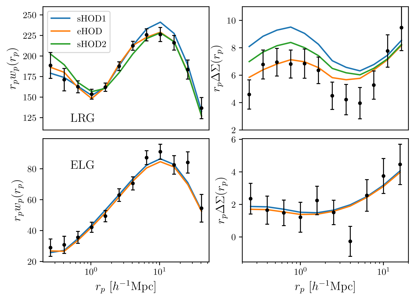
Figure 2: Best fit HOD models for LRG (top) and ELG (bottom) panels. The subscript s/e denotes the standard and extended HOD model. The points with errors bar correspond to the measured $w_{p}$ (left) and $\Delta\Sigma$ (right) signal. The blue lines (sHOD1) correspond to a fit to the projected correlation function $w_{p}$ only, while the green (SHOD2) and orange lines (eHOD) correspond to standard and extended HOD fits including the measurement of $\Delta\Sigma$ in the fitting pipeline. The extended HOD model provides a good description of both the clustering and lensing signal.

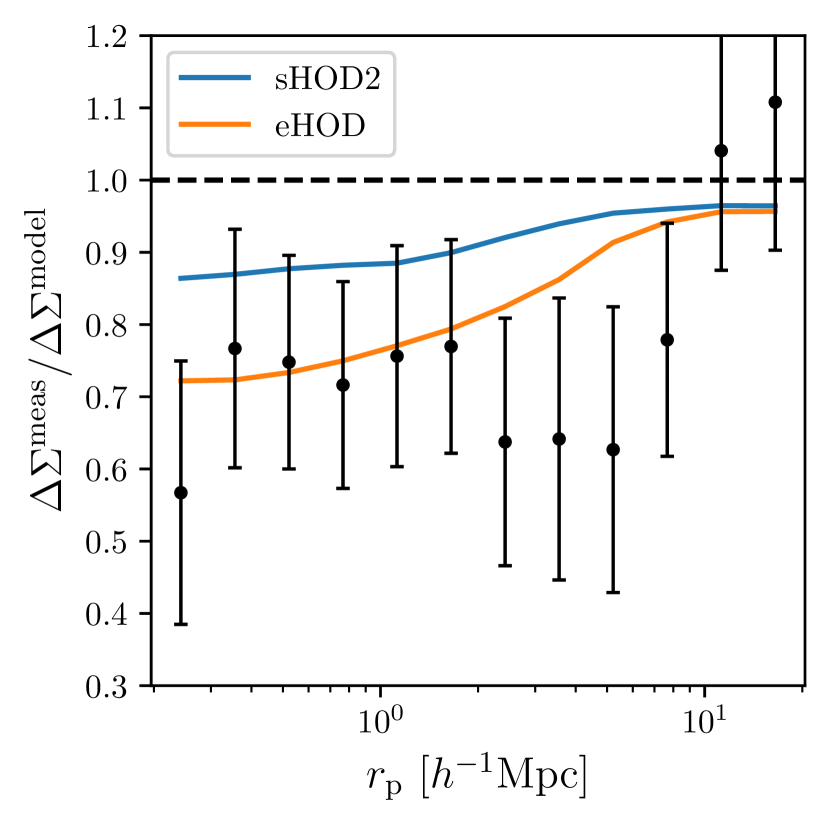
Figure 3: Difference between the observed galaxy-galaxy lensing signal (points with error bars) in eBOSS LRG with the prediction of a standard HOD (sHOD) determined by fitting the projected correlation function $w_{\mathrm{p}}$ only. The continuous line in blue represents an sHOD fit to $w_{\mathrm{p}}+\Delta\Sigma$ while the orange line corresponds to the extended HOD model.

While this method provides a good correction scheme at large scales, which is enough for the study of galaxy anisotropic clustering, it fails on smaller scales, and we therefore need another method to correct for fiber collisions. In particular, we use here the pairwise-inverse probability (PIP) and angular upweighting (ANG) weights described in Mohammad et al. (2020). These weights were shown to properly account for fiber collisions at small separations. However, PIP weights were only produced for eBOSS galaxies, and we therefore only apply ANG weights to the combined sample (including the $cp$ weights), as they are providing sufficient correction below 1 $h^{-1}$Mpc. For $w_{p}(r_{p})$, we use 13 logarithmic bins in $r_{p}$ between 0.2 and 50 $h^{-1}$Mpc, with $\pi_{\mathrm{max}}$ = 80 $h^{-1}$Mpc. In addition to the clustering, we also fit the GGL signal, similarly to the work of Contreras et al. (2023), observed with eBOSS lenses around DES sources in order to further constrain the assembly bias parameters. The measured GGL differential excess surface density is defined as

$$\Delta\Sigma_{\mathrm{gm}}(R)=\bar{\Sigma}_{\mathrm{gm}}(R)-\Sigma_{\mathrm{gm}}(R),$$ (21)

where the mean projected surface density is defined as

$$\bar{\Sigma}_{\mathrm{gm}}(R)=\frac{2}{R^{2}}\int_{0}^{R}\Sigma_{\mathrm{gm}}(r)r\mathrm{d}r.$$ (22)

The projected surface density $\Sigma_{\mathrm{gm}}(r)$ can be written as a function of the galaxy-matter cross-correlation as (Guzik & Seljak, 2001; de la Torre et al., 2017; Jullo et al., 2019)

$$\Sigma_{\mathrm{gm}}(R)=\Omega_{\mathrm{m}}\rho_{\mathrm{c}}\int_{-\infty}^{\infty}\xi_{\mathrm{gm}}\left(\sqrt{R^{2}+\chi^{2}}\right)\mathrm{d}\chi,$$ (23)

with the mean matter density $\rho_{\mathrm{m}}=\Omega_{\mathrm{m}}\rho_{\mathrm{c}}=3\Omega_{\mathrm{m}0}H_{0}^{2}/8\pi G$ constant in redshift in comoving coordinates. The galaxy-matter correlation function is measured in the range [$5\times 10^{-3},150$]$h^{-1}$Mpc with 41 logarithm bins, by cross-correlating galaxy mock catalogs with the dark-matter particles of the simulation, sub-sampled by a factor of 2000. We then estimate $\Sigma_{\mathrm{gm}}(r)$ by integrating up to 100 $h^{-1}$Mpc. The estimation of $\Delta\Sigma$ is then compared to the one observed in the data, which is computed as (Jullo et al., 2019)

$$\Delta\Sigma_{\mathrm{gm}}\left(r_{\mathrm{p}}\right)= \frac{\sum_{\mathrm{l},\mathrm{s}}^{N_{\mathrm{ls}}}\sum_{\mathrm{cr}}\left(z_{1},z_{\mathrm{s}}\right)w_{\mathrm{l},\mathrm{s}}\epsilon_{+}\left(r_{\mathrm{p}}\right)}{\sum_{\mathrm{l},\mathrm{s}}^{N_{\mathrm{l},\mathrm{s}}}w_{\mathrm{l},\mathrm{s}}}$$ (24)

$$-\frac{\sum_{\mathrm{r},\mathrm{s}}^{N_{\mathrm{r},\mathrm{s}}}\sum_{\mathrm{cr}}\left(z_{\mathrm{r}},z_{\mathrm{s}}\right)w_{\mathrm{r},\mathrm{s}}\epsilon_{+}\left(r_{\mathrm{p}}\right)}{\sum_{\mathrm{r},\mathrm{s}}^{N_{\mathrm{r},\mathrm{s}}}w_{\mathrm{r},\mathrm{s}}},$$

Table 1: Best fit parameters for all fit configurations. The baseline eHOD configuration in this work corresponds to the case where the concentration and an annular definition of $\delta$ are used as additional parameters.

Method	sHOD1	sHOD2	eHOD $\delta_{\mathrm{vir}}$,c	eHOD $T^{ij}_{\mathrm{vir}}$,c	eHOD $T^{ij}_{\mathrm{vir}}$, b/a	eHOD $\delta_{\mathrm{annulus}}$,c	eHOD $\delta_{\mathrm{annulus}}$,b/a	eHOD $T^{ij}_{5\mathrm{Mpc}}$ ,c
$M_{\mathrm{min}}$	13.24	12.81	12.95	13.23	12.93	13.03	13.11	13.26
$M_{\mathrm{cut}}$	14.18	13.84	13.91	13.80	13.72	13.76	13.76	13.87
$\sigma$	0.54	0.11	0.44	0.74	0.53	0.58	0.67	0.72
$\alpha$	1.20	1.36	0.91	0.93	1.05	0.93	0.90	0.97
$\kappa$	0.39	0.36	0.64	0.48	0.39	0.56	0.51	0.46
$f_{\mathrm{ic}}$	0.64	0.28	0.32	0.38	0.25	0.30	0.32	0.43
$A_{\mathrm{cent}}$			0.11	- 0.01	0.10	0.18	0.20	0.15
$B_{\mathrm{cent}}$			- 0.27	-0.27	-0.24	-0.25	-0.25	-0.18
$A_{\mathrm{sat}}$			0.01	-0.15	-0.05	-0.06	-0.08	-0.02
$B_{\mathrm{sat}}$			0.00	-0.04	-0.10	0.01	0.02	0.01
$f_{\mathrm{sat}}\%$	8.0	14.1	13.3	12.8	16.6	14.8	14.6	12.0
$\chi^{2}_{r}$	1.05	2.45	1.43	1.11	1.06	1.08	1.09	1.62

where $z_{\mathrm{s}}$ and $z_{\mathrm{l}}$ correspond to the source and lens redshift respectively. The subtraction around random lenses reduces the contribution of lensing systematics and leads to a reduced variance on small scales (Singh et al., 2017). The critical density $\Sigma_{\mathrm{cr}}$ is defined as

$$\Sigma_{\mathrm{cr}}\left(z_{1},z_{\mathrm{s}}\right)=\frac{c^{2}}{4\pi G\left(1+z_{\mathrm{s}}\right)^{2}}\frac{D_{\mathrm{S}}}{D_{\mathrm{LS}}D_{\mathrm{L}}},$$ (25)

where $D_{\mathrm{S}},D_{\mathrm{LS}},D_{\mathrm{L}}$ are the observer-source, lens-source, and observer-lens angular diameter distances. We measured $\Delta\Sigma(r_{p})$ with 13 (11 for the ELGs) logarithmic bins in the range between 0.2 and 20 $h^{-1}$Mpc with the python package dsigma (Lange & Huang, 2022). We used Metacalibration shape measurements and corrected for potential systematic effects induced by this method. We used for photometric redshifts of source galaxies the ones estimated with the Directional Neighbourhood Fitting (DNF) algorithm (De Vicente et al., 2016). Errors in photo-$z$ measurements can lead to bias in the estimation of $\Delta\Sigma$. We matched DES galaxies with galaxies observed spectroscopically with BOSS and eBOSS. While these samples are not representative of DES galaxies, they can however be used to obtain a rough estimate of the bias introduced by the photo-$z$. We found that photo-$z$ leads to an underestimation of the observed signal by approximately $3-5\%$ at all scales. Since this effect is sub-dominant compared to the signal-to-noise (S/N) of our measurements, we do not include it. We also do not include any Boost factor correction Miyatake et al. (2015) as we have found that it has nearly no impact on our measurements, even at the smallest scale.

We then compare the clustering and lensing signal to the observed ones in eBOSS by mean of a likelihood analysis

$$-2\ln\mathcal{L}(\theta)=\sum_{i,j}^{N_{p}}\@vec{\Delta}_{i}(\theta)\hat{\Psi}_{ij}\@vec{\Delta}_{j}(\theta),$$ (26)

where $\theta$ is the set of HOD parameters, $\Delta$ is the data-model difference vector, $N_{p}$ is the total number of data points and $\hat{\Psi}_{ij}$ is the precision matrix, the inverse of the covariance matrix. The covariance matrix is determined by jackknife (JK) subsampling with $N=100$ patches. Since all ELGs are within the DES footprint, we can use the same JK regions for the clustering and lensing measurements in order to estimate the cross-correlation between $w_{\mathrm{p}}$ and $\Delta\Sigma$. For the LRGs, only about a third of the sample is within DES footprint. We decided to use the whole sample to estimate $w_{\mathrm{p}}$, to get a sufficient S/N measurement. Since $\Delta\Sigma$ is only measured within the overlapping footprint, the cross-covariance cannot be estimated through the jackknife method, and we assume it to be zero. We have checked with the ELG sample that this assumption does not change significantly the results: the jackknife cross-covariance is mainly dominated by noise.

Our fitting procedure corresponds to the one described in (Rocher et al., 2023a, b). The parameter space is first sampled with a quasi-uniform grid, which serves as a training sample for a Gaussian process regressor. Here we use the one implemented in sklearn. For each sampled point in the parameter space, the clustering and lensing signals are averaged over ten realizations to reduce stochastic noise from halo occupation. We then repeat iteratively the following procedure: we use an MCMC sampler, here emcee (Foreman-Mackey & al., 2013), to sample our parameter space given our surrogate model generated by the Gaussian process regressor. We then randomly pick 3 points within our final MCMC chains from which we compute the likelihood. We then add these points to the initial training sample and re-train our Gaussian process. In Rocher et al. (2023a), they found that iterating up to $N=800$ from a training sample of $N_{\text{ini}}\approx 1000$ was enough to get robust contours. These findings are highly dependent on the parameter space we want to explore and the dynamic range of the likelihood. While we do find the same conclusion for an ELG-HOD, the degree of degeneracy of a LRG-HOD, calls for a higher number of iterations. We therefore use $N_{\text{ini}}=1000$ (resp. 2000) and $N=1000$ (resp. 2000) for ELG (resp. LRG) fit respectively.

4 Results

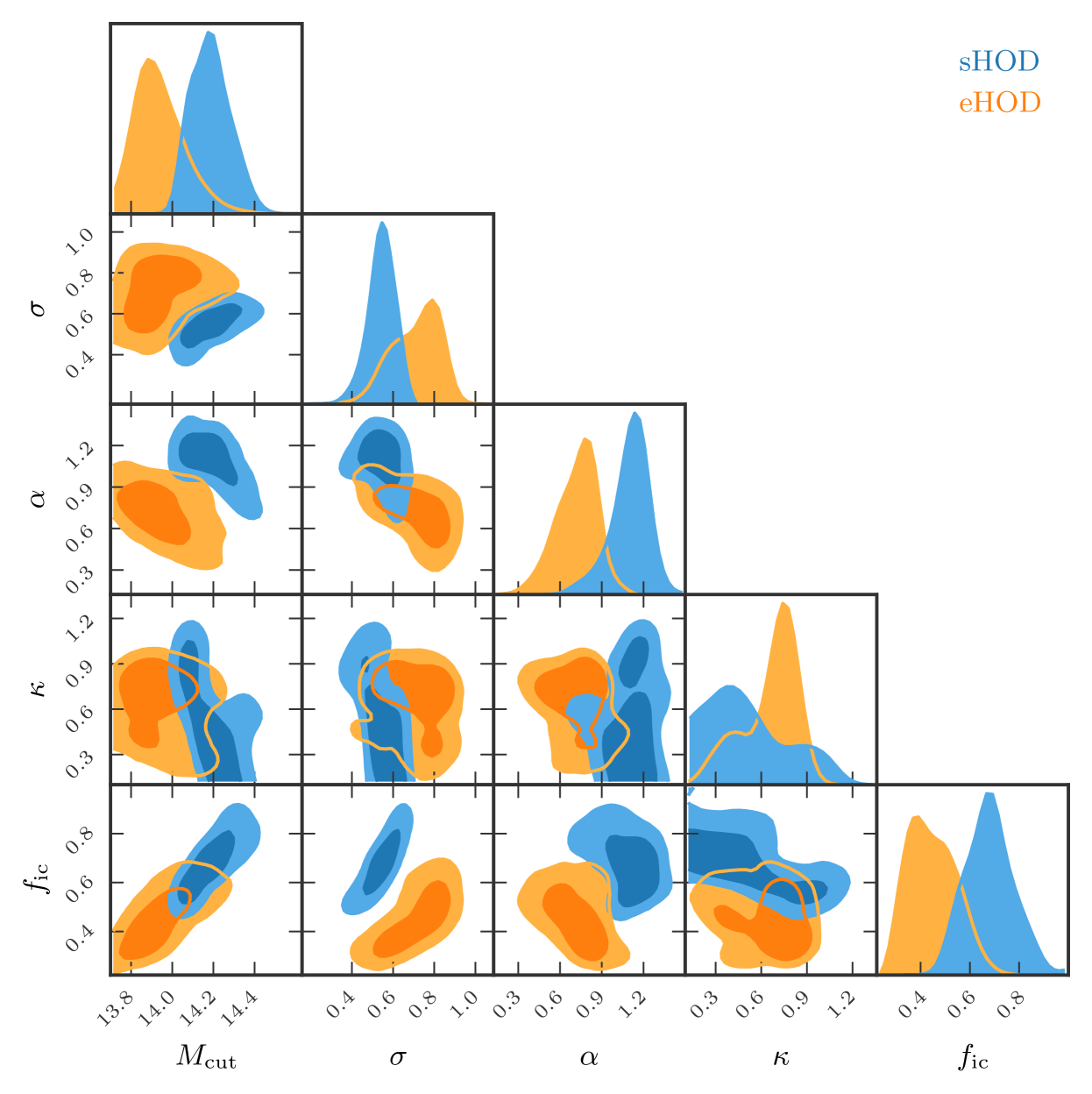
Figure 4: Full posterior distribution of the sHOD (in blue) and eHOD (in orange) in our baseline configuration (including concentration and annular density as additional parameters) for the LRG sample. We can observe that the extra parameters contained in the eHOD model have a strong impact on the posterior distributions

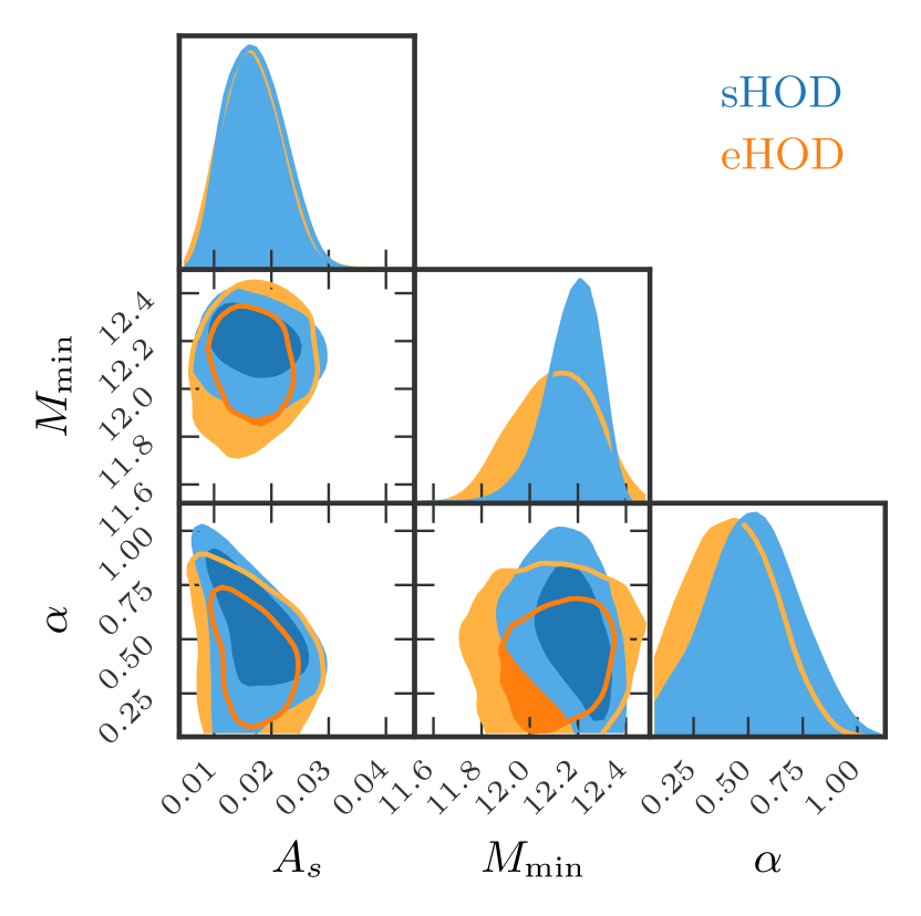
Figure 5: Full posterior distribution for the sHOD (in blue) and eHOD (in orange) models. Taking into account assembly bias parameters has little impact on halo occupation.

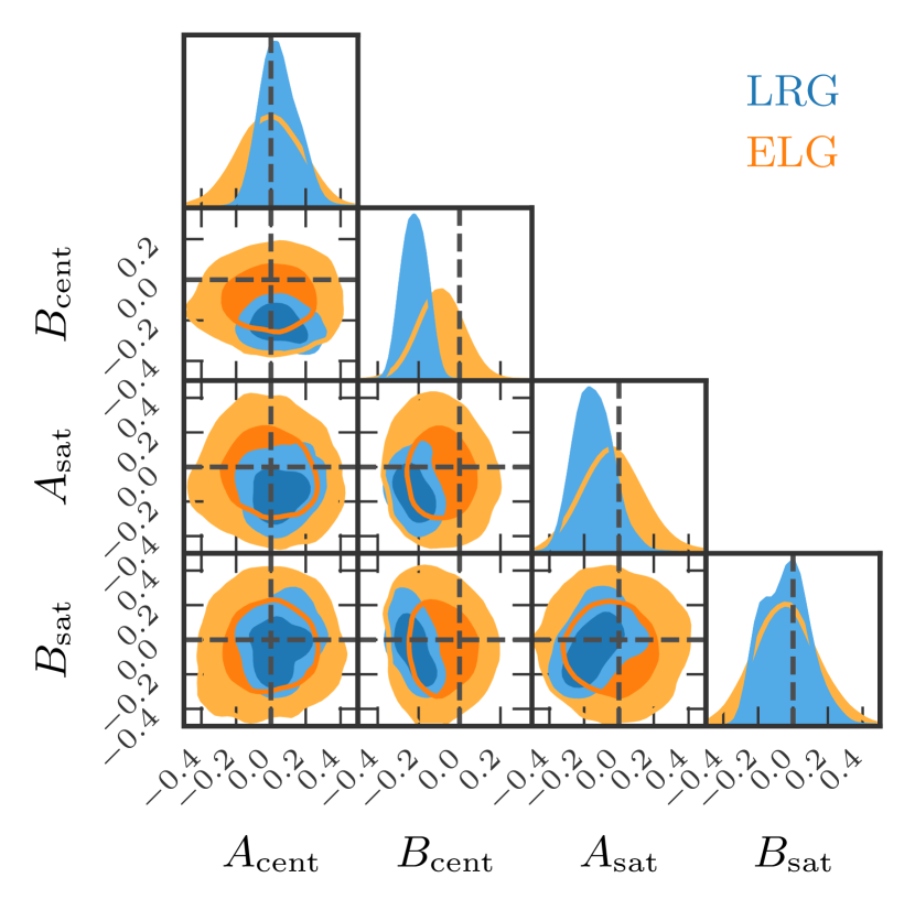
Figure 6: Full posteriors distributions of the assembly bias and environmental parameters in our baseline configuration (see Section 4.1. For the LRGs, the negative value of $B_{\mathrm{cent}}$, detected at $3\sigma$, indicates that LRG centrals most likely occupy a dense environment. A negative value of $A_{\mathrm{sat}}$ at the 1$\sigma$ level, indicates that satellite galaxies could be preferentially located in more concentrated halos than average. For the ELGs, all parameters are consistent with zero at the $1\sigma$ level, suggesting that ELGs do not exhibit significant assembly bias or environmental dependencies.

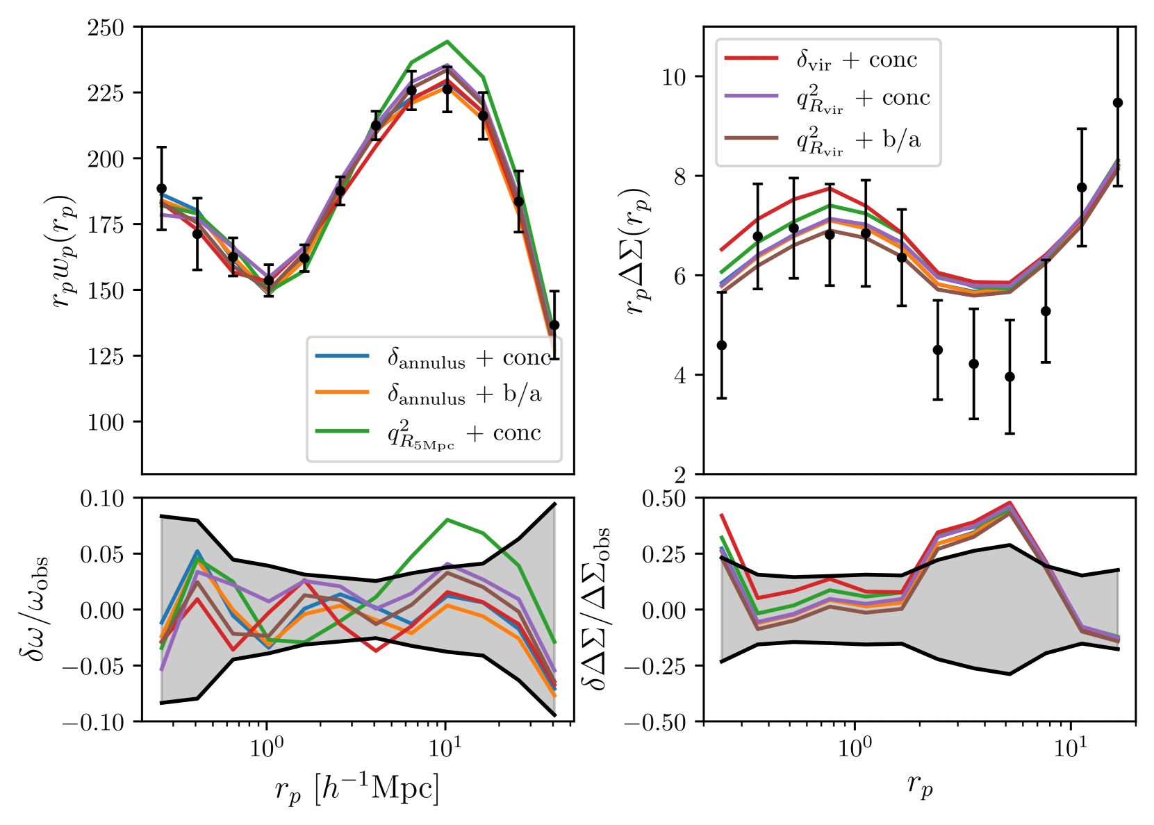
Figure 7: Result for different combinations of assembly bias (concentration and shape) and local environments (density and shear) parameters. Top panels present the measurements while the bottom panels show the relative differences. All the models provide similar best-fitting clustering predictions, lensing predictions and goodness of fit results, except the shear measured with a Gaussian Kernel of size 2.25 $h^{-1}$Mpc which has a slightly worse goodness of fit.

4.1 Luminous Red Galaxies

As a baseline configuration for the extended HOD (eHOD) model, we use the concentration as a proxy of assembly bias and the local density, described as an annular definition of the density field $\delta$, following the formalism of Yuan et al. (2022). We present in Fig. 2 the best-fit results obtained with the standard (s) and extended (e) HOD models. The standard model sHOD2 and the extended model both fit the combined $w_{p}$, $\Delta\Sigma$ data vector, while the sHOD1 model only fits $w_{p}$. Best-fit values are given in Table 1 while full posterior distributions and prior information can be found in Fig. 4, Fig. 6 and in Appendix A. For the sHOD1, we can see that the model over-predicts the signal at scales around 10 $h^{-1}\mathrm{Mpc}$ while obtaining a satellite fraction of $8\%$, slightly lower than those obtained in Alam et al. (2020); Yuan et al. (2022) and $50\%$ below the best-fit value of Zhai et al. (2017). We found that this difference was due to noise in the jackknife covariance estimate of $w_{\mathrm{p}}$. When we performed a fit only considering the diagonal elements, we obtained a satellite fraction of $11\%$, the model matches well the peak at 10 $h^{-1}\mathrm{Mpc}$ but in turn provides a poor fit at scales $1-3h^{-1}\mathrm{Mpc}$, similarly to the observed fit for the sHOD2 case, an issue in the modeling also reported in Zhai et al. (2017).

The introduction of secondary HOD parameters enables us to provide a good description of the small and intermediate scales of $w_{\mathrm{p}}$, while also yielding a more accurate description of $\Delta\Sigma$, decreasing the reduced chi-square from $\chi^{2}_{r}=2.45$ down to $\chi^{2}_{r}=1.08$, an improvement mainly due to a better description of $\Delta\Sigma$ on the scales below 3 $h^{-1}$ Mpc. This is illustrated in Fig. 3, which displays the ratio of $\Delta\Sigma$ measurements in the data and as measured in the mocks generated by sHOD2 and eHOD models (calibrated on both $w_{p}$ and $\Delta\Sigma$ measurements), compared to the $\Delta\Sigma$ measurement as measured in the mock generated by the sHOD1 (calibrated only against the projected clustering $w_{p}$). The standard model dashed line) over-predicts the GGL signal by $30-40\%$ at scales below 10$h^{-1}$ Mpc, while a combined fit (blue solid line) poorly alleviates this issue, with a slight improvement of only $\approx 5-15\%$. By considering additional parameters describing internal and external properties of the halos (orange solid line), the modeling of the clustering and lensing signals at small scales is significantly improved compared to using the standard HOD model, with the main improvements coming from the dependence on the local density environment (Yuan et al., 2021; Hadzhiyska et al., 2023a). On scales between $2-10h^{-1}$ Mpc, we observe an improvement of the extended model of 20$\%$ while it matches the data at lower scales, providing a better goodness of fit to the observed lensing signal. Thus, adding secondary halo parameters to the HOD models helps to reproduce the lensing signal at small scales, and gives a partial answer to the ’lensing is low’ problem. Indeed, baryonic feedback, not considered in this work, smoothes out the matter distribution, also contributing to a decrease of $\Delta\Sigma$ (Amodeo et al., 2021). This better description can be achieved in the model by lowering the mass threshold above which central and satellite galaxies occupy dark matter halos. To maintain a similar galaxy bias, galaxies in lower mass halos should therefore be located in higher density peaks. This is what we obtain in the posterior distributions of Fig. 6. A negative value of $B_{\mathrm{cent}}$ implies that halos located in denser environments are more likely to be populated, as a decrease of $M_{\mathrm{min}}^{\mathrm{mod}}$ in Eq. 17 increases the probability of populating such halos, a result also found for CMASS galaxies (Yuan et al., 2022) and in hydrodynamical simulations (Artale et al., 2018).

Our results also suggest that central LRGs preferentially populate halos of low concentration, as we obtained a positive best-fit value for $A_{\mathrm{cent}}$ = 0.18 (see Table 1), while Yuan et al. (2022) find an opposite trend for the CMASS sample when fitting $\xi(r_{\perp},r_{\parallel})$. In recent studies, halo occupation was found to be strongly dependent on formation time (Zehavi et al., 2018; Artale et al., 2018), and concentration (Bose et al., 2019; Delgado et al., 2022), as both are tightly linked to one another Wechsler et al. (2002). These results show that, at low mass, central galaxies are more likely to be hosted by more concentrated, early-formed halos, this trend reverses at higher mass due to the contributions of satellite galaxies. For the satellite occupation, there seems to be a slight correlation with concentration, with satellite galaxies most likely to be hosted in more concentrated halos. This is in disagreement with the results of Bose et al. (2019): at all halos mass, concentrated halos have fewer satellite galaxies, as they had more time to merge with the central. However, given our measurements, the only parameter that is well constrained is $B_{\mathrm{cent}}$, being non-zero at the 3$\sigma$ level, while all the other parameters are consistent with zero at the 1$\sigma$ level. Similarly to Yuan et al. (2022), we also find that including secondary assembly bias parameters (or just fitting $\Delta\Sigma$) does increase the satellite fraction. This can be explained by the fact that central-particle correlation is dominant on small scales (Leauthaud et al., 2017), which causes the fit to naturally provide higher $f_{\mathrm{sat}}$ values. For completeness, we present the full posterior distribution of the extended HOD in Appendix B.

Table 2: Posterior and best-fit results for the ELG HOD. We show here the 16$\%$, 50$\%$, and 84$\%$ percentiles of the posterior distribution. The first column presents the prior ranges for each parameter. The two other columns show the 16$\%$, 50$\%$ and 84$\%$ percentiles of the posterior distributions, with the best-fit values in parenthesis defined as the minimum of the $chi^{2}$ of the MCMC chains, for both sHOD and eHOD models. The initial value of $A_{c}$ is fixed to 0.01 meaning that $A_{s}$ is allowed to vary in the range [0.2,20]$A_{c}$. Other columns present the rescaled values of $A_{c}$ and $A_{s}$ in order to match the ELG number density. For the sHOD, we show in parenthesis the reduced chi-square including $\Delta\Sigma$.

Method	sHOD	eHOD
$A_{s}$ [0.002,0.02]	$0.017^{+0.006}_{-0.005}$(0.015)	$0.017^{+0.006}_{-0.005}$(0.015)
$M_{\mathrm{min}}$ [11.5,12.5]	$12.19^{+0.10}_{-0.12}$ (12.28)	$12.11^{+0.17}_{-0.19}$(12.21)
$\sigma$ [0.1,1.2]	$0.52^{+0.23}_{-0.23}$(0.41)	$0.42^{+0.22}_{-0.23}$(0.28)
$A_{\mathrm{cent}}$ [-0.5,0.5]		$-0.01^{+0.19}_{-0.22}$ (-0.08)
$B_{\mathrm{cent}}$ [-0.5,0.5]		$-0.09^{+0.11}_{-0.19}$ (-0.04)
$A_{\mathrm{sat}}$ [-0.5,0.5]		$-0.04^{+0.19}_{-0.18}$ (0.02)
$B_{\mathrm{cent}}$ [-0.5,0.5]		$-0.04^{+0.20}_{-0.12}$(-0.08)
$A_{c}$ [0.01]	$0.034^{+0.012}_{-0.011}$ (0.047)	$0.028^{+0.017}_{-0.012}$ (0.038)
$f_{\mathrm{sat}}\%$	10.4	13.3
$\chi^{2}_{r}$	1.13(1.22)	1.40

4.2 Emission Line Galaxies

The best-fit results for ELGs are represented on the bottom panel of Fig. 2 while the posterior contours are shown in Fig. 5 with the corresponding constraints in Table 2. We do not observe significant differences between the standard and the extended HOD framework, when either considering the best-fit model or the full posterior distribution. Both models provide similar goodness of fit and reproduce the observations, with a $\chi^{2}$ = 23.1(22.0) for the sHOD and eHOD models respectively, resulting in a worst reduced $\chi^{2}$ for the eHOD, as the four additional free parameters do not significantly improve the fit. From the posterior distributions in Fig. 6, we can see that all the secondary parameters are consistent with zero at the $1\sigma$ level. In the literature, it was shown that ELGs are preferentially located in higher dense regions than average (Artale et al., 2018; Delgado et al., 2022) and in more concentrated halos (Zehavi et al., 2018; Artale et al., 2018; Rocher et al., 2023b). This is in agreement with our negative best-fit values for $A_{\mathrm{cent}}$ and $B_{\mathrm{cent}}$, even though we cannot derive more decisive conclusions from our analysis.

In addition, we find a satellite fraction of $10.4\%$ for the sHOD, significantly lower than that reported in Avila et al. (2020), $f_{\mathrm{sat}}=22\%$. However, for ELGs the mean satellite occupation is independent of that of the centrals, which means that an ELG satellite can orbit around a non-ELG central. Thus, it only contributes to the two-halo term of the ELG correlation function, affecting the amplitude of the linear bias of the galaxy sample. The lower satellite fraction (compared to Avila et al. (2020)) can be explained by the fact that our mean value for $M_{\mathrm{min}}=12.19$ is larger than that reported in Avila et al. (2020), $M_{\mathrm{min}}=11.71$, and that we allow $\alpha$ to vary (resulting in a different satellite occupation over halo mass). In Rocher et al. (2023b), when they include strict conformity, i.e. satellite galaxies can only populate halo in the presence of a central ELG, they reported a very small fraction of satellite of $\approx 2-3\%$. For DESI ELGs, strict conformity is needed in order to provide a positive value for $\alpha$, which is predicted by semi-analytical models Gonzalez-Perez et al. (2018, 2020).

4.3 Dependence on parameter choices

We present in Fig. 7 multiple eHOD best-fit models for different configurations. We tested as environment proxy either the local shear or the local density, combined with internal properties, i.e. concentration or shape of the dark matter halos. As a reminder, the baseline configuration corresponds to the case where we apply to Eq. 17, $f_{A}$ = concentration and $f_{B}=\delta_{\mathrm{annulus}}$, with $\delta_{\mathrm{annulus}}$ calculated by counting neighboring halos. Estimating the local density field with this definition provides a better description of the observed LRG signal, with a $\chi_{\mathrm{r}}^{2}$ improved by $\Delta\chi^{2}_{\mathrm{r}}$ = -1.39 compared to the case where the density field is estimated on a mesh with a Gaussian smoothing kernel of size = $2.25r_{\mathrm{vir}}$, with $\Delta\chi^{2}_{\mathrm{r}}$ = -0.98. These results are in agreement with those of Yuan et al. (2022) who found that estimating the density field with a Gaussian kernel of a fixed size of 3 $h^{-1}$ Mpc yields no significant improvement compared to the sHOD. Using instead of the concentration, the shape of the dark-matter halo as a proxy for assembly bias provides nearly indistinguishable best-fit model results. The resulting constraints, presented in Table 1 and in Appendix B, suggest that red galaxies preferentially occupy more ellipsoidal halos than average, as the best-fitting value $A_{\mathrm{cent}}$ is positive when either considering shear or density as external property. The two extra configurations including the local density are in agreement with the baseline configuration, in favor of a negative value for $B_{\mathrm{cent}}$, such that galaxies preferentially occupy more dense environment.
Using the local shear instead of the local density also provides good $\chi_{\mathrm{r}}^{2}$ values when the tidal tensor is computed with a Gaussian kernel of size 2.25 $r_{\mathrm{vir}}$. The best $\chi_{\mathrm{r}}^{2}$ value is obtained when combining the local shear with the halo shape, $\chi_{\mathrm{r}}^{2}$ = 1.06. It better reproduces the small scales of $\Delta\Sigma$ but gives a slightly worse fit around the peak of $w_{\mathrm{p}}$ observed at $10h^{-1}$ Mpc. Surprisingly, using the local shear with a fixed Gaussian smoothing of size 2.25 $h^{-1}$Mpc provides the worst $\chi_{\mathrm{r}^{2}}$ value out of all configurations. This demonstrates that local density anisotropy should be considered at halo scales to retrieve the maximum amount of information, as explained in Paranjape et al. (2018). Our results suggest that galaxies preferentially occupy more anisotropic environments, in agreement with Delgado et al. (2022) that found this correlation for low-mass halos, and with DESI ELG Rocher et al. (2023b).

4.4 Cosmological fit

In current analysis, perturbative and semi-analytical models that aim at extracting cosmological information from the observations, are tested intensively against galaxy mock catalogs. In eBOSS analysis, different HOD models were used in order to quantify modeling systematics of redshift-space distortions models (Rossi et al., 2021; Alam et al., 2021). The authors found consistent results amongst a large variety of HOD models which validated the accuracy of the theoretical models. In the work of de la Torre et al. (2017); Jullo et al. (2019), the measured anisotropic clustering $\xi(r_{\perp},r_{\parallel})$ at an effective redshift $z$, is combined at the likelihood level with lensing measurements of $\Delta\Sigma$ in order to provide direct constraints on $f(z)$, the growth rate of structure, $\sigma_{8}(z)$ the amplitude of matter fluctuation and $\Omega_{\mathrm{m}}$, the present time matter density. These studies extract information at scales below 3 $h^{-1}$Mpc where our HOD models, as illustrated in Fig. 2, show significant differences which might introduce biases when quantifying modeling systematics of $\Delta\Sigma$.

Here, we perform the cosmological analysis of galaxy catalogs populated with the standard and extended HOD framework in order to test the accuracy of a combined analysis of galaxy clustering and galaxy-galaxy lensing. We consider as a redshift space model the Taruya et al. (2010) model extended to non-linearly biased tracers, hereafter referred to as TNS, described and robustly tested in detail in Bautista et al. (2021). The expression for the redshift space power spectrum of biased tracers is given by

$$P^{s}(k,\nu)=D(k\nu\sigma_{v})\big{[}P_{\rm gg}(k)+2\nu^{2}fP_{\rm{g}\theta}(k)+\nu^{4}f^{2}P_{\theta\theta}(k)+\\ C_{A}(k,\nu,f,b_{1})+C_{B}(k,\nu,f,b_{1})\big{]},$$ (27)

where $k$ is the wave-vector norm, $\nu$ is the cosine angle between the wave-vector and the line of sight, $\theta$ is the divergence of the velocity field $\mathbf{v}$ defined as $\theta=-\nabla{\bf\cdot v}/(aHf)$, and $f$ is the linear growth rate parameter. $C_{A}(k,\nu,f)$ and $C_{B}(k,\nu,f)$ are the two correction terms given in Taruya et al. (2010), which reduce to one-dimensional integrals of the linear matter power spectrum. The damping function $D(k\nu\sigma_{v})$ describes the Finger-of-God effect induced by random motions in virialized systems, inducing a damping effect on the power spectra. We adopted a Lorentzian form, $D(k,\nu,\sigma_{v})=(1+k^{2}\nu^{2}\sigma_{v}^{2}/2)^{-2}$, where $\sigma_{v}$ represents an effective pairwise velocity dispersion treated as an extra nuisance parameter. The expressions of the real space quantities $P_{\mathrm{gg}},P_{\mathrm{g}\theta}$ and $P_{\mathrm{gm}}$ are given following the bias expansion formalism of Assassi et al. (2014)

$$P_{\mathrm{gg}}(k)= b_{1}^{2}P_{\delta\delta}(k)+b_{2}b_{1}I_{\delta^{2}}(k)+2b_{1}b_{\mathcal{G}_{2}}I_{\mathcal{G}_{2}}(k)$$ (28)

$$+2\left(b_{1}b_{\mathcal{G}_{2}}+\frac{2}{5}b_{1}b_{\Gamma_{3}}\right)F_{\mathcal{G}_{2}}(k)+\frac{1}{4}b_{2}^{2}I_{\delta^{2}\delta^{2}}(k)$$

$$+b_{\mathcal{G}_{2}}^{2}I_{\mathcal{G}_{2}\mathcal{G}_{2}}(k)\frac{1}{2}b_{2}b_{\mathcal{G}_{2}}I_{\delta_{2}\mathcal{G}_{2}}(k),$$

$$P_{\mathrm{g}\theta}(k)= b_{1}P_{\delta\theta}(k)+\frac{b_{2}}{2}I_{\delta^{2}\theta}(k)+b_{\mathcal{G}_{2}}I_{\mathcal{G}_{2}\theta}(k)$$

$$+\left(b_{\mathcal{G}_{2}}+\frac{2}{5}b_{\Gamma_{3}}\right)F_{\mathcal{G}_{2}\theta}(k),$$

$$P_{\mathrm{gm}}(k)= b_{1}P_{\delta\delta}(k)+\frac{b_{2}}{4}I_{\delta^{2}}(k)+b_{\mathcal{G}_{2}}I_{\mathcal{G}_{2}}(k)$$

$$+\left(b_{\mathcal{G}_{2}}+\frac{2}{5}b_{\Gamma_{3}}\right)F_{\mathcal{G}_{2}}(k),$$

where each function of $k$ is a 1-loop integral of the linear matter power spectrum $P_{\mathrm{lin}}$, which expression can be found in Simonović et al. (2018). The expressions of $I_{\delta^{2}\theta}(k)$, $I_{\mathcal{G}_{2}\theta}(k)$ and $F_{\mathcal{G}_{2}\theta}(k)$ are the same as $I_{\delta^{2}}(k)$, $I_{\mathcal{G}_{2}}(k)$ and $F_{\mathcal{G}_{2}}(k)$ except than the $G_{2}$ kernel replaces the $F_{2}$ kernel in the integrals. To estimate the velocity divergence power spectra $P_{\theta\theta}$ and $P_{\delta\theta}$, we used Bel et al. (2019) fitting function, that depends solely on $\sigma_{8}$,

$$P_{\theta\theta}(k)=P_{L}(k)e^{-k\left(a_{1}+a_{2}k+a_{3}k^{2}\right)},$$ (29)

$$P_{\delta\theta}(k)=\left(P_{\delta\delta}(k)P_{\text{lin }}(k)\right)^{\frac{1}{2}}e^{-\frac{k}{k_{\delta}}-bk^{6}},$$

with the expressions of each parameter given in Bel et al. (2019); Bautista et al. (2021). The linear matter power spectrum is estimated with camb (Lewis & Challinor, 2011) while the non-linear power spectrum $P_{\delta\delta}$ is estimated with the latest version of HMcode (Mead et al., 2021). This is different from Bautista et al. (2021); Paviot et al. (2022) where we used the response function formalism respresso described in Nishimichi et al. (2017). Indeed the latest version of HMcode provides a nearly indistinguishable (at least in configuration space) baryon acoustic oscillations damping due to non-linear effects, while also matching at higher $k$ the power spectrum of respresso.

The TNS correlation function multipole moments are finally determined by performing the Hankel transform of the model power spectrum multipole moments,

$$\xi^{\mathrm{TNS}}_{\ell}(s)=i^{\ell}\frac{2\ell+1}{2}\int\mathrm{d}k\frac{k^{2}}{2\pi^{2}}j_{\ell}(ks)\int_{-1}^{1}\mathrm{d}\nu\,P^{s}(k,\nu)L_{\ell}(\nu),$$ (30)

where $j_{\ell}$ and $L_{\ell}$ denote the spherical Bessel function and Legendre polynomials of order $\ell$. The Hankel transform, i.e. the outer integral in the above equation, is performed rapidly using FFTLog algorithm (Hamilton, 2000).

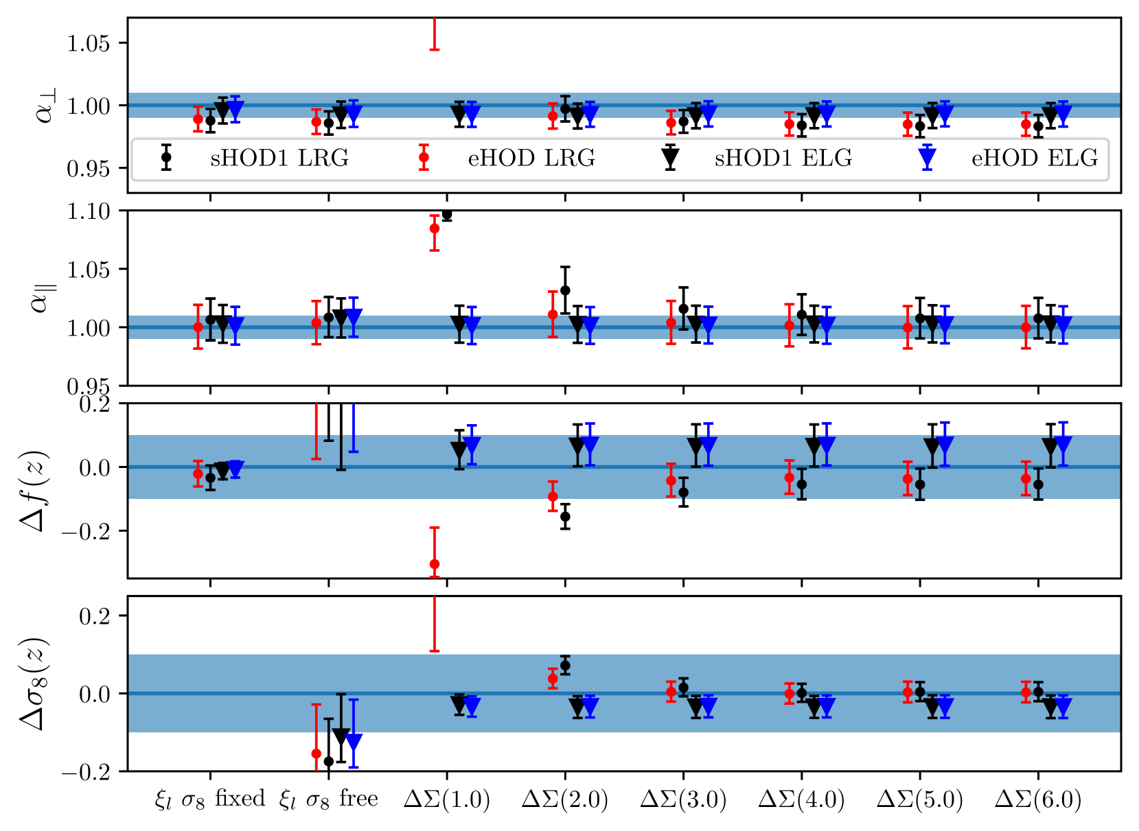
Figure 8: Results from the cosmological fit. Circle points with error bars correspond to the fit of LRG catalog at redshift $z=0.70$ populated with the standard and extended HOD framework while the triangles correspond to the fit of ELGs at redshift $z=0.86$. The value of $f$ and $\sigma_{8}$ for LRG(ELG) are 0.814(0.849) and 0.570(0.529) at the redshift $z=0.70(0.86)$. Values in parenthesis correspond to the minimum scale used in the fit in $h^{-1}\mathrm{Mpc}$. The shaded area corresponds to a $10\%$ variation around the fiducial value of each parameter.

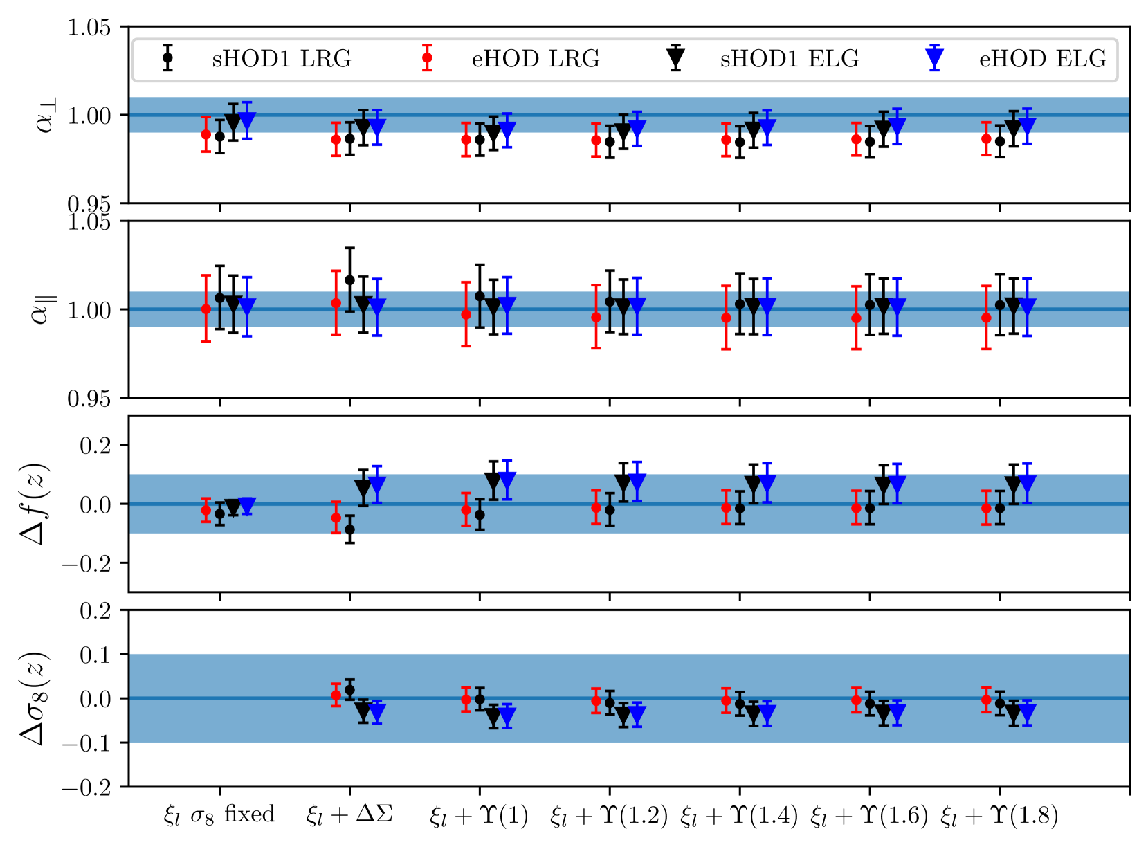
Figure 9: Same as Fig. 8, but this time considering the annular excess surface density $\Upsilon$ instead.

Under the limber approximation Limber (1953), the expression of the galaxy-galaxy lensing signal is given by Marian et al. (2015)

$$\Delta\Sigma_{\mathrm{gm}}(r_{\mathrm{p}})=\rho_{\mathrm{m}}\int\frac{\mathrm{d}^{2}k_{\perp}}{(2\pi)^{2}}P_{\mathrm{gm}}\left(k_{\perp},z_{l}\right)J_{2}\left(k_{\perp}R\right),$$ (31)

with $J_{2}$ the second order Bessel function of first kind and $\rho_{\mathrm{m}}$ the comoving matter density. In order to remove the contribution of non-linear modes, we computed the annular differential excess surface density (ASAD) estimator given by (Baldauf et al., 2010)

$$\Upsilon\left(r_{\mathrm{p}},R_{0}\right)=\Delta\Sigma_{\mathrm{gm}}\left(r_{\mathrm{p}}\right)-\left(\frac{R_{0}}{r_{\mathrm{p}}}\right)^{2}\Delta\Sigma_{\mathrm{gm}}\left(R_{0}\right),$$ (32)

where $R_{0}$ corresponds to a cut-off radius, below which scale the signal is damped.

In addition, we parametrize the Alcock-Paczyński (AP) distortions (Alcock & Paczynski, 1979) induced by the assumed fiducial cosmology in the measurements via two dilation parameters that scale transverse, $\alpha_{\perp}$, and radial, $\alpha_{\parallel}$, separations. These quantities are related to the comoving angular diameter distance, $D_{M}=(1+z)D_{A}(z)$, and Hubble distance, $D_{H}=c/H(z)$, respectively, as

$$\alpha_{\perp} =\frac{D_{M}(z_{\rm eff})}{D_{M}^{\rm fid}(z_{\rm eff})},$$ (33)

$$\alpha_{\parallel} =\frac{D_{H}(z_{\rm eff})}{D_{H}^{\rm fid}(z_{\rm eff})},$$ (34)

where $c$ is the speed of light in the vacuum, and $z_{\rm eff}$ is the effective redshift of the sample. We apply these dilation parameters to the theoretical TNS power spectrum $P^{s}(k,\nu)$ in Eq. 30, so that $P^{s}(k,\nu)\rightarrow P^{s}(k^{\prime},\nu^{\prime})$ where

$$k^{\prime} = \frac{k}{\alpha_{\perp}}\left[1+\nu^{2}\left(\frac{1}{F_{\rm AP}^{2}}-1\right)\right]^{1/2},$$ (35)

$$\nu^{\prime}\ = \frac{\nu}{F_{\rm AP}}\left[1+\nu^{2}\left(\frac{1}{F_{\rm AP}^{2}}-1\right)\right]^{-1/2},$$ (36)

and $F_{\rm AP}=\alpha_{\parallel}/\alpha_{\perp}$. $\Delta\Sigma$ and $\Upsilon$, being projected quantities, are only distorted by the perpendicular distortion factor

$$\Delta\Sigma(R^{\prime}) =\Delta\Sigma(\alpha_{\perp}R),$$ (37)

$$\Upsilon(R^{\prime}) =\Upsilon(\alpha_{\perp}R).$$

Given a theoretical model for $\xi_{\ell}$ and $\Delta\Sigma$ ($\Upsilon$), we can perform a cosmological analysis assuming a Gaussian likelihood as defined in Eq. 26. Here, our data vector is the combined multipoles galaxy-galaxy lensing signal, with the free parameters of the model $\theta\subset(b_{1},b_{2},b_{\Gamma_{3}},f,\sigma_{8},\alpha_{\perp},\alpha_{\parallel},\sigma_{v})$, $b_{\mathcal{G}_{2}}$ being fixed to Lagrangian prescription as $b_{\mathcal{G}_{2}}=-2/7(b_{1}-1)$ (Saito et al., 2014). It is worth noting that, as the TNS corrections and the galaxy biased expansion are functions of the linear power spectrum only, these can be rescaled at each iteration by the normalization $\sigma_{8}$. The non-linear power spectrum evaluated with HMcode is first sampled into a broad range of $\sigma_{8}$ and then interpolated at any value of $\sigma_{8}$ within our prior, such that the only quantities that we re-computed at each iteration are the real space quantities $P_{\theta\theta}$ and $P_{\delta\theta}$. We will assume as fiducial cosmology the cosmology of the Uchuu simulation, such that AP distortions should be equal to unity.

The covariance matrix is estimated with analytical prescriptions. The Gaussian covariance for the multipoles of the correlation function is given by (Grieb et al., 2016)

$$C_{\ell_{1}\ell_{2}}^{\xi}\left(s_{i},s_{j}\right)=\frac{i^{\ell_{1}+\ell_{2}}}{2\pi^{2}}\int_{0}^{\infty}k^{2}\sigma_{\ell_{1}\ell_{2}}^{2}(k)\bar{\jmath}_{\ell_{1}}\left(ks_{i}\right)\bar{\jmath}_{\ell_{2}}\left(ks_{j}\right)\mathrm{d}k,$$ (38)

where the $\bar{\jmath}_{\ell}$ correspond to bin-averaged spherical bessel functions,

$$\bar{\jmath}_{\ell}\left(ks_{i}\right)\equiv\frac{4\pi}{V_{s_{i}}}\int_{s_{i}-\Delta s/2}^{s_{i}+\Delta s/2}s^{2}j_{\ell}(ks)\mathrm{d}s,$$ (39)

with $V_{si}$ the volume element of the shell. The expression for $\sigma_{\ell_{1}\ell_{2}}^{2}(k)$ is given by

$$\sigma_{\ell_{1}\ell_{2}}^{2}(k)\equiv \frac{\left(2\ell_{1}+1\right)\left(2\ell_{2}+1\right)}{V_{\mathrm{s}}}$$ (40)

$$\times\int_{-1}^{1}\left[P(k,\mu)+\frac{1}{\bar{n}}\right]^{2}\mathcal{L}_{\ell_{1}}(\mu)\mathcal{L}_{\ell_{2}}(\mu)\mathrm{d}\mu,$$

with $V_{s}$ the volume of the periodic box. The expression for the Gaussian covariance of $\Delta\Sigma$ is given by Marian et al. (2015)

$$\operatorname{Cov}[\widehat{\Delta\Sigma}]\left(R_{i},R_{j}\right)=\frac{1}{A_{s}}\left(\rho_{m}^{0}\right)^{2}\int\frac{\mathrm{d}^{2}k_{\perp}}{(2\pi)^{2}}\bar{J}_{2}\left(k_{\perp}R_{i}\right)\bar{J}_{2}\left(k_{\perp}R_{j}\right)$$ (41)

$$\times\left\{\left[P_{\delta\delta}\left(k_{\perp}\right)+\frac{1}{\bar{n}_{p}}\right]\left[P_{\mathrm{gg}}\left(k_{\perp}\right)+\frac{1}{\bar{n}_{g}}\right]+P_{\mathrm{gm}}^{2}\left(k_{\perp}\right)\right\},$$

Table 3: Result of the cosmological fit from the optimal configurations determined from Fig. 8 and from Fig. 9 for the extended HOD model.

Parameter	$\Delta\alpha_{\perp}$	$\Delta\alpha_{\parallel}$	$\Delta f$	$\Delta\sigma_{8}$
LRG $\xi_{\ell}$ $\sigma_{8}$ fixed	$-0.012\pm 0.010$	$0.006\pm 0.018$	$-0.035\pm 0.039$
LRG $\xi_{\ell}$ $\sigma_{8}$ free	$-0.013\pm 0.010$	$0.003\pm 0.018$	$0.325\pm 0.277$	$-0.155\pm 0.099$
LRG $\xi_{\ell}$ + $\Delta\Sigma$ $r_{\mathrm{min}}=3h^{-1}$Mpc	$-0.013\pm 0.009$	$0.004\pm 0.017$	$-0.048\pm 0.051$	$0.007\pm 0.026$
LRG $\xi_{\ell}$ + $\Upsilon$ $r_{0}=1.2h^{-1}$Mpc	$-0.014\pm 0.009$	$-0.002\pm 0.017$	$-0.014\pm 0.054$	$-0.003\pm 0.028$
ELG $\xi_{\ell}$ $\sigma_{8}$ fixed	$-0.004\pm 0.010$	$0.002\pm 0.016$	$-0.012\pm 0.026$
ELG $\xi_{\ell}$ $\sigma_{8}$ free	$-0.007\pm 0.010$	$0.008\pm 0.017$	$0.341\pm 0.257$	$-0.128\pm 0.077$
ELG $\xi_{\ell}$ + $\Delta\Sigma$ $r_{\mathrm{min}}=1h^{-1}$Mpc	$-0.007\pm 0.010$	$0.001\pm 0.015$	$0.062\pm 0.057$	$-0.033\pm 0.025$
ELG $\xi_{\ell}$ + $\Upsilon$ $r_{0}=1h^{-1}$Mpc	$-0.008\pm 0.010$	$0.001\pm 0.016$	$0.072\pm 0.062$	$-0.035\pm 0.027$

where $A_{s}$ is the surface area of the box. The $\bar{J}_{2}$ correspond to bin-averaged Bessel functions, computed in the same way as in Eq. 39 by integrating over the surface element instead. In Eqs 38-41, we assume linear theory for the power spectra, such that $P_{\delta\delta}=P_{\mathrm{lin}}$, $P_{\mathrm{gm}}=b_{1}P_{\delta\delta}$, $P_{\mathrm{gg}}=b_{1}^{2}P_{\delta\delta}$ and $P(k,\mu)=b_{1}^{2}P_{\mathrm{gg}}(k)\left(1+\beta^{2}\mu^{2}\right)^{2}$ (Kaiser, 1987), with $\beta=f/b$. We infer the value of $f$ from the uchuu cosmology at the effective redshift of the LRG and ELG sample, respectively $z=0.7$ and $z=0.86$, while the value of $b_{1}$ are taken from Bautista et al. (2021); Tamone et al. (2020). The shot-noise terms $\bar{n}_{p}$ and $\bar{n}_{g}$ correspond to the number density of dark-matter particles and galaxies in the simulation box. No analytical cross-covariance exists between $\Delta\Sigma$ and the $\xi_{\ell}$ such that we approximate it to be zero. To estimate the covariance of $\Upsilon$, we generate a sample of a thousand $\Delta\Sigma$ from a multivariate normal distribution, given the $\Delta\Sigma$ covariance estimate. We then apply Eq. 32 to each fake sample by considering its mean value for $\Delta\Sigma(R_{0})$. this has the effect of reducing noise in the final covariance estimation.

We measured the multipoles of the correlation function with bins of size 5 $h^{-1}$ Mpc in the range between 0 and 150 $h^{-1}$ Mpc. $\Delta\Sigma$ is measured with 22(16) logarithm bins in the range between $10^{-1}$ and $10^{2}$ $h^{-1}$ Mpc for LRGs and ELGs respectively. This binning was chosen for each sample given the S/N of the observations. We perform fit of the multipoles on scales between 25 and 140 $h^{-1}$ Mpc, with a minimum scale determined from the analysis of Bautista et al. (2021), as it provides unbiased constraints on cosmological parameters.

Here, we test the accuracy of the TNS model as a function of different minimum scales used when fitting either $\Delta\Sigma$ or $\Upsilon$. The maximum scale that we used here is 80 $h^{-1}$ Mpc as Limber approximation breaks down on larger scales. We present in Fig. 8 the results of the emcee MCMC chains of the combined $\xi_{\ell}+\Delta\Sigma$ fit and in Table 3 the corresponding constraints. As expected, we obtain unbiased constraints when fitting only the clustering while fixing the value of $\sigma_{8}(z)$ to the fiducial value of the simulation. However, in the scenario where $\sigma_{8}$ is allowed to vary, we can observe a strong degeneracy between $f$ and $\sigma_{8}$ that is not captured properly by the model given the amount of information present in the multipoles. It is only when combining anisotropic clustering with galaxy-galaxy lensing measurements that one can break this degeneracy.

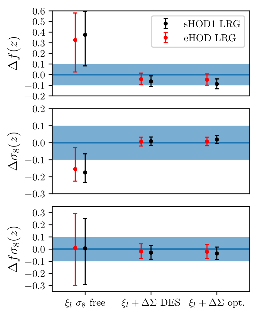
Figure 10: Comparison between a fit to the multipoles $\xi_{\ell}$ only (left) and a fit to the combined $\xi_{\ell}+\Delta\Sigma$ data vector. We present constraints for the scale cuts used for $\gamma_{t}$ in the DES y3 analysis (Krause et al., 2021), $r_{\mathrm{min}}$ = 6 $h^{-1}$Mpc and for the optimal configuration determined in this work, $r_{\mathrm{min}}$ = 3 $h^{-1}$Mpc.

For the LRG mocks, our model provides unbiased constraints on each cosmological parameter, regardless of the HOD, on scales above $3h^{-1}$ Mpc for $\Delta\Sigma$, with the constraints on the eHOD which seems to converge faster toward consistent results. This is surprising, given the observed difference in Fig. 2. The main difference comes from the goodness of fit, with the TNS model providing a better description of the $\Delta\Sigma$ measured with the eHOD galaxy population, $\Delta\chi^{2}\approx 20$ compared to the sHOD. The fact that the TNS model provides a good fit, $\chi^{2}_{r}=0.8$, of the eHOD measurements suggests that our model is also capable of yielding a good description of the observations down to scale of $\approx$ 3 $h^{-1}$Mpc, in agreement with the result of de la Torre et al. (2017), even if baryonic feedback that affects the shape of $\Delta\Sigma$ up to these scales, are not considered in the modeling.

For ELGs, we can see that both HOD models provide indistinguishable constraints from one another, as both methods provide very similar clustering and lensing measurements. Surprisingly, we find that the model provides unbiased and consistent constraints over all the considered range down to $r_{\mathrm{min}}$ = 1$h^{-1}$Mpc. This means that our estimator of $P_{\mathrm{gm}}$, which is built upon a one-loop biased expansion of the non-linear matter power spectrum estimated with HMcode, is valid up to non-linear scales to describe ELGs, at least at an effective redshift of $z=0.86$. This might be related to their spatial distribution, indeed Gonzalez-Perez et al. (2020) found that half of DESI ELGs reside in filaments and a third in sheets, where density fluctuations are small compared to the nodes where LRGs usually lie. This is consistent with the results of Hadzhiyska et al. (2021) who found that it was twice more likely for ELG to reside in sheets compared to a mass-selected sample. In addition, ELGs occupy lower mass halos, $\log M\approx 12.2h^{-1}M_{\odot}$, compared to LRGs, with $\log M$ in the range $12.8-13.2h^{-1}M_{\odot}$, such that the 1-halo term contribution to $\Delta\Sigma$ is excepted to be smaller for ELGs at around $1h^{-1}$Mpc. This explains why our bias perturbative expansion provides a good description of the galaxy-galaxy lensing signal of the ELGs down to small scales. As baseline configuration, we adopt $r_{\mathrm{min}}=1(3)h^{-1}$Mpc for ELGs and LRGs respectively.

Our analysis demonstrates the constraining power of $\Delta\Sigma$, in combination with anisotropic clustering measurements, as illustrated in Fig. 10. This methodology provides unbiased constraints on the cosmological parameters $\alpha_{\perp},\alpha_{\parallel},f$ and $\sigma_{8}$, improving the precision compared to a $\xi_{\ell}$ fit only by a factor of about 6 and 3 for $f$ and $\sigma_{8}$ respectively. However, let us emphasize that this conclusion is obviously optimistic, as the variance in observation is dominated by the shape noise contribution Gatti et al. (2021) which is not considered in this work. We compare the optimal LRG configuration determined in this work, $r_{\mathrm{min}}=3h^{-1}$Mpc to the one determined in DES analysis (Krause et al., 2021), $r_{\mathrm{min}}=6h^{-1}$Mpc. We observe similar constraints for the two configurations, with a small $3\%$ improvement in precision for $\sigma_{8}$. As we move down to highly non-linear scales, the two-point function captures less and less information, such that the gain in precision becomes smaller.

We present in Fig. 9 the results of the fits when combining the $\xi_{\ell}$ with $\Upsilon$, compared to the baseline configuration determined from Fig. 8. Since the ELG fits for $\Delta\Sigma$ provide consistent results up to 1$h^{-1}$Mpc, the constraints when fitting $\Upsilon$ should be the same, regardless of the value of $R_{0}$, which is exactly what we observe on this figure. The trend is similar for LRGs, with consistent results when fitting $\Upsilon$ with a value of $R_{0}$ above $1.2h^{-1}$Mpc. As baseline configuration we therefore adopt $R_{0}=1(1.2)h^{-1}$Mpc for ELGs and LRGs respectively. We present in Table 3 the corresponding constraints with our baseline configuration for $\Delta\Sigma$ and $\Upsilon$. Both methods provide similar constraints with consistent results at the 1 $\sigma$ level. The difference in $\chi^{2}$ is smaller between the extended and standard framework, $\Delta\chi^{2}=5$, as observed differences in $\Delta\Sigma$ are smoothed out with the annular excess surface density estimator. It seems that some information is lost when using $\Upsilon$ as a proxy for galaxy-galaxy lensing since the constraints on $f$ and $\sigma_{8}$ are larger by 5 to 8$\%$. However, this effect is marginal, below $1\%$, compared to the statistical precision. We therefore conclude that both statistics, either $\Delta\Sigma$ or $\Upsilon$, can be used interchangeably when doing a joint cosmological analysis of galaxy clustering and lensing.

5 Conclusion

In this paper, we revisit the extended HOD framework introduced in Yuan et al. (2022), built on top of the state-of-art uchuu simulation. This HOD model includes internal (halo concentration and shape) and environmental (local density and local shear) dependencies of central and satellite occupation. We apply this model to two eBOSS tracers: the emission lines galaxies (ELGs) in the range $0.6<z<1.1$, and the luminous red galaxies (LRGs) in the range $0.6<z<1.0$, by modelling the projected correlation $w_{p}$ and the galaxy-galaxy lensing signal $\Delta\Sigma$ from highly non-linear ($\approx$ Mpc scale) up to linear scales.
We find that the extended HOD model provides a better description of both the clustering and lensing signal of LRGs, reducing the observed discrepancy on $\Delta\Sigma$ from 30-40 $\%$ to 0-20$\%$ compared to the standard HOD model based on halo mass only. Our results demonstrate the necessity to include in the HOD framework environment-based secondary parameters with a strong detection, at the 3$\sigma$ level, that LRGs preferentially occupy anisotropic and denser environments. As internal halo property, we have tested either the concentration and shape of the dark-matter halo, and we have found that both properties can be used to improve the HOD model. For ELGs, we find given our statistical precision, that either the standard or extended HOD framework provides consistent and robust modeling for both the clustering and lensing signal, with a slight preference for ELGs living in denser regions, in agreement with previous results Artale et al. (2018); Delgado et al. (2022).

We then conducted a cosmological analysis of the redshift-space correlation function and galaxy-galaxy lensing signal for both HOD frameworks using a perturbative model. For LRGs, we find that our model provides unbiased and consistent constraints on the linear growth rate $f$, on the amplitude of fluctuations $\sigma_{8}$ and on the Alcock-Paczynski parameters on scales above 3$h^{-1}$Mpc and 1.2$h^{-1}$Mpc when fitting the galaxy-galaxy lensing signal $\Delta\Sigma$ and the annular excess surface density $\Upsilon$ respectively. In addition, we find that our model provides a better description of the extended HOD framework, suggesting that the observed eBOSS galaxy-galaxy lensing signal can be accurately modeled down to scales below $5h^{-1}$Mpc, where significant discrepancies can be observed between the HODs and the data. Moreover, we find for ELGs that we can derive robust constraints from the galaxy-galaxy lensing signal down to very small scales, $r_{\mathrm{min}}=1.0h^{-1}$Mpc, regardless of the estimator of the galaxy-galaxy lensing signal. This analysis will serve as a cornerstone for a companion paper that will extract cosmological information from eBOSS galaxy-galaxy lensing signal and pave the way for future cosmological analysis of joint clustering and galaxy-galaxy lensing measurement for future cosmological experiments such as DESI, EUCLID or VRO/LSST.

Appendix A Additional parameters

We present in Fig. 11 the normalized distribution in the range [-1,1] of internal (concentration and ellipticity) and external (local density and local shear) halo properties on the left and right panel respectively. We present in Fig. 12 the relation between the two different local density estimators described in this work.

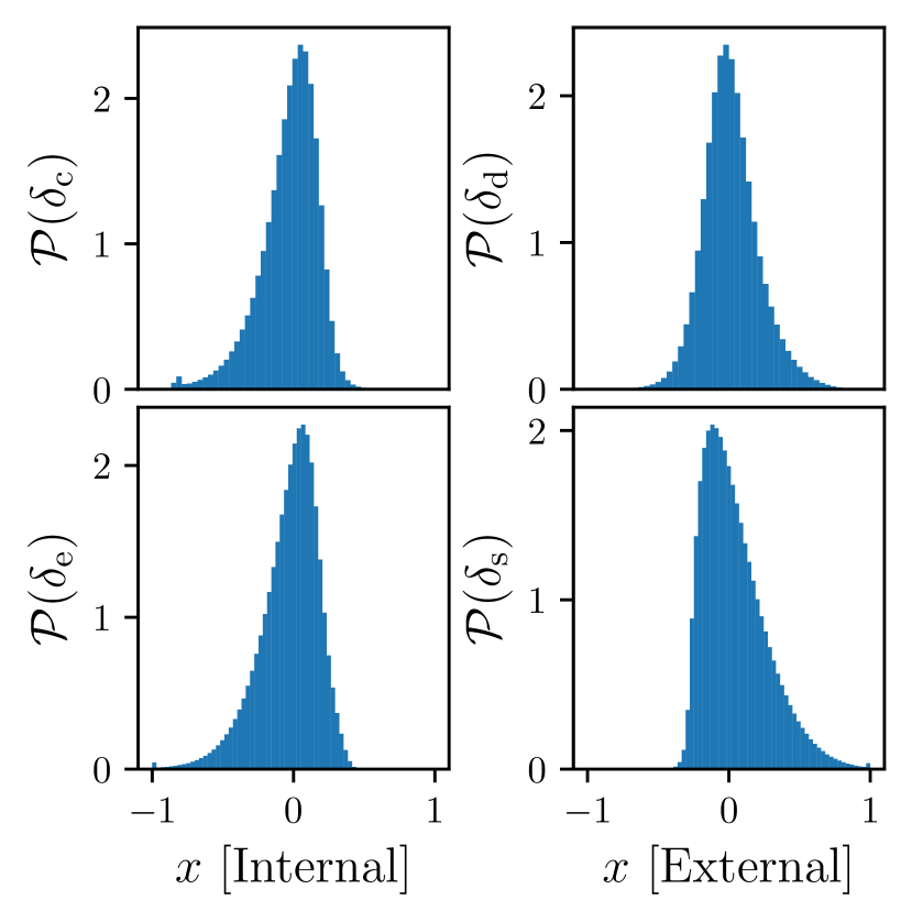
Figure 11: Distribution of internal and external halo properties as defined in Sec 3.2. The left panels present the distribution of concentration (c) and ellipticity (e) while the right panels present the local density (d) and local shear (s).

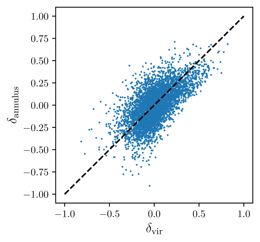
Figure 12: Comparison between the local density estimated on a mesh with a Gaussian filter of size $R$ = 2.25 $r_{\mathrm{vir}}$ and the local density estimated by counting halo and sub-halo around $r_{\mathrm{vir}}$ and 5 $h^{-1}$Mpc.

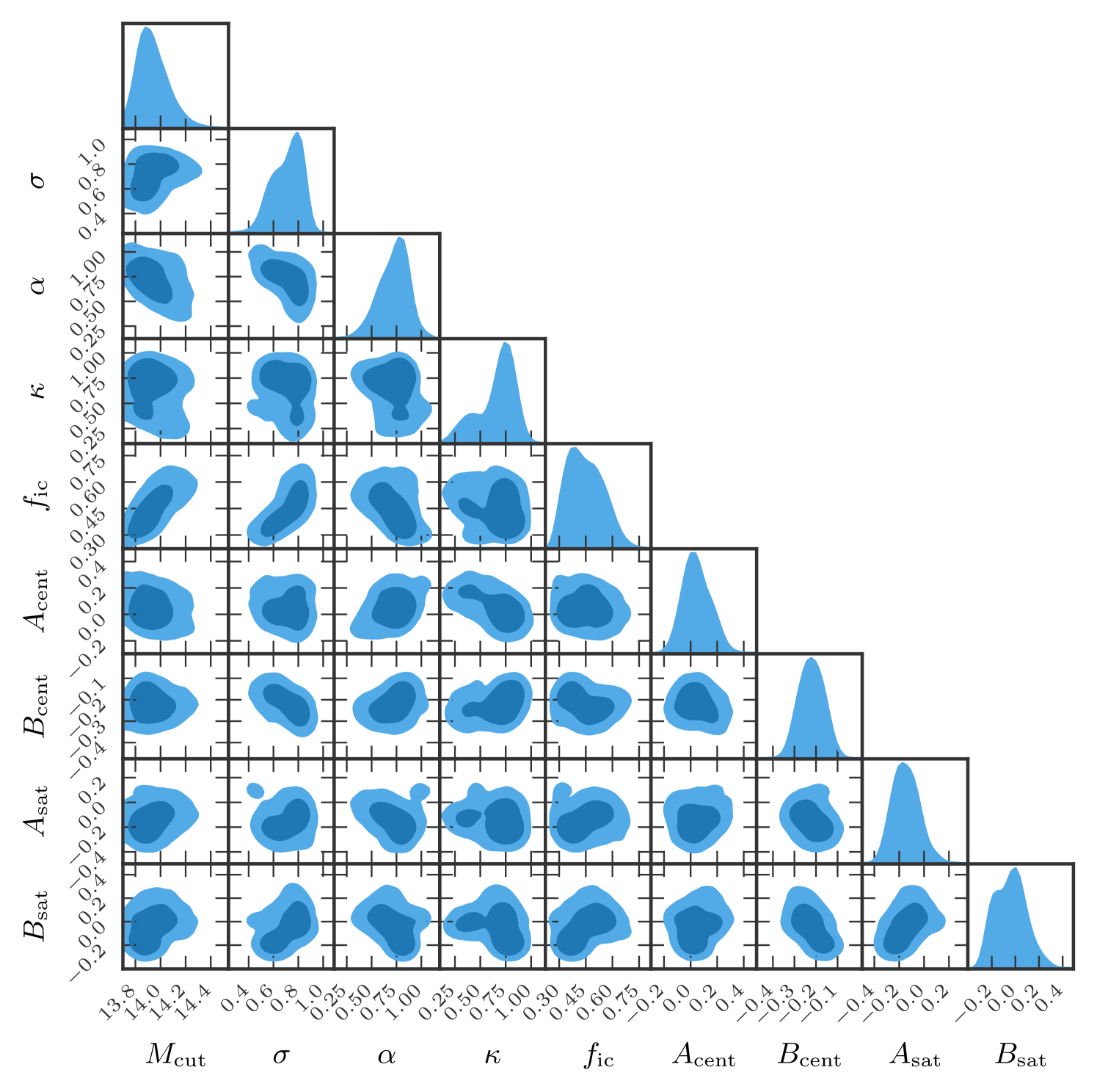
Figure 13: Full posteriors distribution of the LRG extended HOD, including the assembly bias parameters.

Table 4: Result of the Gaussian process emulating the likelihood function after 4000 iterations for the eBOSS LRG sample. We present here the $16\%$, $50\%$ and $84\%$ percentiles of the posterior distributions. The prior are presented in bracket and correspond to uniform priors within the quoted ranges.

Method	sHOD1	sHOD2	eHOD $\delta_{\mathrm{vir}}$,c	eHOD $T^{ij}_{\mathrm{vir}}$,c	eHOD $T^{ij}_{\mathrm{vir}}$,b/a	eHOD $\delta_{\mathrm{annulus}}$ ,c	eHOD $\delta_{\mathrm{annulus}}$,b/a	eHOD $T^{ij}_{5\mathrm{Mpc}}$ ,c
$M_{\mathrm{cut}}$ [13.7,15.0]	$14.17^{+0.13}_{-0.12}$	$14.02^{+0.07}_{-0.06}$	$14.02^{+0.12}_{-0.09}$	$13.91^{+0.15}_{-0.14}$	$13.86^{+0.10}_{-0.09}$	$13.92^{+0.14}_{-0.11}$	$13.91^{+0.12}_{-0.11}$	$13.94^{+0.13}_{-0.11}$
$\sigma$ [0.1,1.2]	$0.53^{+0.11}_{-0.12}$	$0.40^{+0.11}_{-0.13}$	$0.50^{+0.11}_{-0.13}$	$0.77^{+0.10}_{-0.12}$	$0.65^{+0.13}_{-0.13}$	$0.74^{+0.09}_{-0.14}$	$0.79^{+0.11}_{-0.10}$	$0.79^{+0.10}_{-0.09}$
$\alpha$ [0.1,1.5]	$1.11^{+0.14}_{-0.15}$	$1.12^{+0.16}_{-0.10}$	$0.83^{+0.20}_{-0.20}$	$0.83^{+0.15}_{-0.14}$	$0.92^{+0.13}_{-0.19}$	$0.73^{+0.14}_{-0.18}$	$0.82^{+0.11}_{-0.11}$	$1.02^{+0.09}_{-0.16}$
$\kappa$ [0.1,1.5]	$0.59^{+0.30}_{-0.31}$	$0.72^{+0.21}_{-0.22}$	$0.79^{+0.13}_{-0.16}$	$0.29^{+0.29}_{-0.15}$	$0.73^{+0.20}_{-0.32}$	$0.69^{+0.14}_{-0.31}$	$0.58^{+0.26}_{-0.32}$	$0.45^{+0.16}_{-0.12}$
$f_{\mathrm{ic}}$ [0.1,1.0]	$0.64^{+0.20}_{-0.15}$	$0.45^{+0.10}_{-0.07}$	$0.41^{+0.08}_{-0.07}$	$0.42^{+0.15}_{-0.18}$	$0.34^{+0.08}_{-0.07}$	$0.45^{+0.11}_{-0.10}$	$0.43^{+0.10}_{-0.09}$	$0.45^{+0.09}_{-0.07}$
$A_{\mathrm{cent}}$ [-0.5,0.5]			$-0.01^{+0.15}_{-0.12}$	$0.24^{+0.23}_{-0.31}$	$0.01^{+0.19}_{-0.13}$	$0.04^{+0.14}_{-0.10}$	$0.12^{+0.24}_{-0.16}$	$0.26^{+0.15}_{-0.38}$
$B_{\mathrm{cent}}$ [-0.5,0.5]			$-0.24^{+0.09}_{-0.08}$	$-0.27^{+0.10}_{-0.09}$	$-0.20^{+0.07}_{-0.06}$	$-0.23^{+0.06}_{-0.06}$	$-0.26^{+0.07}_{-0.08}$	$-0.20^{+0.06}_{-0.06}$
$A_{\mathrm{sat}}$ [-0.5,0.5]			$0.13^{+0.20}_{-0.31}$	$-0.21^{+0.36}_{-0.18}$	$-0.02^{+0.24}_{-0.14}$	$-0.14^{+0.12}_{-0.11}$	$0.01^{+0.16}_{-0.32}$	$-0.10^{+0.12}_{-0.24}$
$B_{\mathrm{sat}}$ [-0.5,0.5]			$-0.08^{+0.11}_{-0.09}$	$0.20^{+0.14}_{-0.27}$	$-0.08^{+0.21}_{-0.10}$	$-0.02^{+0.12}_{-0.15}$	$0.04^{+0.21}_{-0.22}$	$0.04^{+0.08}_{-0.10}$
$M_{\mathrm{min}}$	$13.28^{+0.09}_{-0.09}$					$13.27^{+0.14}_{-0.17}$

Appendix B Posterior of the LRG HOD

We present here the full posterior distributions for the different configurations presented in Section 4.3. We only present $M_{\mathrm{min}}$ for the posterior distributions presented in Fig. 4 to save computational time, as $M_{\mathrm{min}}$ is not a free parameter and is computed for each point of the chain given Eq. 9. In addition, for completeness, we also present the full posterior contours.

References

- Abbott et al. (2022) Abbott, T. M. C., Aguena, M., Alarcon, A., et al. 2022, Phys. Rev. D, 105, 023520
- Alam et al. (2021) Alam, S., de Mattia, A., Tamone, A., et al. 2021, MNRAS, 504, 4667
- Alam et al. (2020) Alam, S., Peacock, J. A., Kraljic, K., Ross, A. J., & Comparat, J. 2020, MNRAS, 497, 581
- Alcock & Paczynski (1979) Alcock, C. & Paczynski, B. 1979, Nature, 281, 358
- Amodeo et al. (2021) Amodeo, S., Battaglia, N., Schaan, E., et al. 2021, Phys. Rev. D, 103, 063514
- Artale et al. (2018) Artale, M. C., Zehavi, I., Contreras, S., & Norberg, P. 2018, MNRAS, 480, 3978
- Assassi et al. (2014) Assassi, V., Baumann, D., Green, D., & Zaldarriaga, M. 2014, J. Cosmology Astropart. Phys., 2014, 056
- Avila et al. (2020) Avila, S., Gonzalez-Perez, V., Mohammad, F. G., et al. 2020, MNRAS, 499, 5486
- Baldauf et al. (2010) Baldauf, T., Smith, R. E., Seljak, U. c. v., & Mandelbaum, R. 2010, Phys. Rev. D, 81, 063531
- Bautista et al. (2021) Bautista, J. E., Paviot, R., Vargas Magaña, M., et al. 2021, MNRAS, 500, 736
- Behroozi et al. (2013) Behroozi, P. S., Wechsler, R. H., & Wu, H.-Y. 2013, ApJ, 762, 109
- Bel et al. (2019) Bel, J., Pezzotta, A., Carbone, C., Sefusatti, E., & Guzzo, L. 2019, A&A, 622, A109
- Berlind & Weinberg (2002) Berlind, A. A. & Weinberg, D. H. 2002, ApJ, 575, 587
- Bose et al. (2019) Bose, S., Eisenstein, D. J., Hernquist, L., et al. 2019, MNRAS, 490, 5693
- Chaves-Montero et al. (2023) Chaves-Montero, J., Angulo, R. E., & Contreras, S. 2023, MNRAS, 521, 937
- Contreras et al. (2023) Contreras, S., Chaves-Montero, J., & Angulo, R. E. 2023, MNRAS, 525, 3149
- Dalal et al. (2008) Dalal, N., White, M., Bond, J. R., & Shirokov, A. 2008, ApJ, 687, 12
- Dark Energy Survey Collaboration et al. (2016) Dark Energy Survey Collaboration, Abbott, T., Abdalla, F. B., et al. 2016, MNRAS, 460, 1270
- Dawson et al. (2016) Dawson, K. S., Kneib, J.-P., Percival, W. J., et al. 2016, AJ, 151, 44
- Dawson et al. (2013) Dawson, K. S., Schlegel, D. J., Ahn, C. P., et al. 2013, AJ, 145, 10
- de la Torre et al. (2017) de la Torre, S., Jullo, E., Giocoli, C., et al. 2017, A&A, 608, A44
- de Mattia et al. (2021) de Mattia, A., Ruhlmann-Kleider, V., Raichoor, A., et al. 2021, MNRAS, 501, 5616
- De Vicente et al. (2016) De Vicente, J., Sánchez, E., & Sevilla-Noarbe, I. 2016, MNRAS, 459, 3078
- Delgado et al. (2022) Delgado, A. M., Wadekar, D., Hadzhiyska, B., et al. 2022, MNRAS, 515, 2733
- Feldman et al. (1994) Feldman, H. A., Kaiser, N., & Peacock, J. A. 1994, ApJ, 426, 23
- Foreman-Mackey & al. (2013) Foreman-Mackey, D. & al. 2013, Publications of the Astronomical Society of the Pacific, 125, 306
- Gatti et al. (2021) Gatti, M., Sheldon, E., Amon, A., et al. 2021, MNRAS, 504, 4312
- Gil-Marín et al. (2020) Gil-Marín, H., Bautista, J. E., Paviot, R., et al. 2020, MNRAS, 498, 2492
- Gonzalez-Perez et al. (2018) Gonzalez-Perez, V., Comparat, J., Norberg, P., et al. 2018, MNRAS, 474, 4024
- Gonzalez-Perez et al. (2020) Gonzalez-Perez, V., Cui, W., Contreras, S., et al. 2020, MNRAS, 498, 1852
- Górski et al. (2005) Górski, K. M., Hivon, E., Banday, A. J., et al. 2005, ApJ, 622, 759
- Gouin et al. (2019) Gouin, C., Gavazzi, R., Pichon, C., et al. 2019, A&A, 626, A72
- Grieb et al. (2016) Grieb, J. N., Sánchez, A. G., Salazar-Albornoz, S., & Dalla Vecchia, C. 2016, MNRAS, 457, 1577
- Guzik & Seljak (2001) Guzik, J. & Seljak, U. 2001, MNRAS, 321, 439
- Hadzhiyska et al. (2020) Hadzhiyska, B., Bose, S., Eisenstein, D., Hernquist, L., & Spergel, D. N. 2020, MNRAS, 493, 5506
- Hadzhiyska et al. (2023a) Hadzhiyska, B., Eisenstein, D., Hernquist, L., et al. 2023a, MNRAS, 524, 2507
- Hadzhiyska et al. (2023b) Hadzhiyska, B., Hernquist, L., Eisenstein, D., et al. 2023b, MNRAS, 524, 2524
- Hadzhiyska et al. (2021) Hadzhiyska, B., Tacchella, S., Bose, S., & Eisenstein, D. J. 2021, MNRAS, 502, 3599
- Hamilton (2000) Hamilton, A. J. S. 2000, MNRAS, 312, 257
- Ishiyama et al. (2009) Ishiyama, T., Fukushige, T., & Makino, J. 2009, PASJ, 61, 1319
- Ishiyama et al. (2012) Ishiyama, T., Nitadori, K., & Makino, J. 2012, arXiv e-prints, arXiv:1211.4406
- Ishiyama et al. (2021) Ishiyama, T., Prada, F., Klypin, A. A., et al. 2021, MNRAS, 506, 4210
- Jullo et al. (2019) Jullo, E., de la Torre, S., Cousinou, M. C., et al. 2019, A&A, 627, A137
- Kaiser (1984) Kaiser, N. 1984, ApJ, 284, L9
- Kaiser (1987) Kaiser, N. 1987, MNRAS, 227, 1
- Krause et al. (2021) Krause, E., Fang, X., Pandey, S., et al. 2021, arXiv e-prints, arXiv:2105.13548
- Landy & Szalay (1993) Landy, S. D. & Szalay, A. S. 1993, ApJ, 412, 64
- Lange & Huang (2022) Lange, J. & Huang, S. 2022, dsigma: Galaxy-galaxy lensing Python package, Astrophysics Source Code Library, record ascl:2204.006
- Leauthaud et al. (2017) Leauthaud, A., Saito, S., Hilbert, S., et al. 2017, MNRAS, 467, 3024
- Lewis & Challinor (2011) Lewis, A. & Challinor, A. 2011, CAMB: Code for Anisotropies in the Microwave Background, Astrophysics Source Code Library, record ascl:1102.026
- Limber (1953) Limber, D. N. 1953, ApJ, 117, 134
- Marian et al. (2015) Marian, L., Smith, R. E., & Angulo, R. E. 2015, MNRAS, 451, 1418
- Mead et al. (2021) Mead, A. J., Brieden, S., Tröster, T., & Heymans, C. 2021, MNRAS, 502, 1401
- Miyatake et al. (2015) Miyatake, H., More, S., Mandelbaum, R., et al. 2015, ApJ, 806, 1
- Mohammad et al. (2020) Mohammad, F. G., Percival, W. J., Seo, H.-J., et al. 2020, MNRAS, 498, 128
- Musso et al. (2018) Musso, M., Cadiou, C., Pichon, C., et al. 2018, MNRAS, 476, 4877
- Myles et al. (2021) Myles, J., Alarcon, A., Amon, A., et al. 2021, MNRAS, 505, 4249
- Navarro et al. (1996) Navarro, J. F., Frenk, C. S., & White, S. D. M. 1996, ApJ, 462, 563
- Nishimichi et al. (2017) Nishimichi, T., Bernardeau, F., & Taruya, A. 2017, Phys. Rev. D, 96, 123515
- Paranjape et al. (2018) Paranjape, A., Hahn, O., & Sheth, R. K. 2018, MNRAS, 476, 3631
- Paviot et al. (2022) Paviot, R., de la Torre, S., de Mattia, A., et al. 2022, MNRAS, 512, 1341
- Planck Collaboration et al. (2016) Planck Collaboration, Ade, P. A. R., Aghanim, N., et al. 2016, A&A, 594, A13
- Rocher et al. (2023a) Rocher, A., Ruhlmann-Kleider, V., Burtin, E., & de Mattia, A. 2023a, J. Cosmology Astropart. Phys., 2023, 033
- Rocher et al. (2023b) Rocher, A., Ruhlmann-Kleider, V., Burtin, E., et al. 2023b, arXiv e-prints, arXiv:2306.06319
- Ross et al. (2020) Ross, A. J., Bautista, J., Tojeiro, R., et al. 2020, MNRAS, 498, 2354
- Rossi et al. (2021) Rossi, G., Choi, P. D., Moon, J., et al. 2021, MNRAS, 505, 377
- Saito et al. (2014) Saito, S., Baldauf, T., Vlah, Z., et al. 2014, Phys. Rev. D, 90, 123522
- Sevilla-Noarbe et al. (2021) Sevilla-Noarbe, I., Bechtol, K., Carrasco Kind, M., et al. 2021, ApJS, 254, 24
- Simonović et al. (2018) Simonović, M., Baldauf, T., Zaldarriaga, M., Carrasco, J. J., & Kollmeier, J. A. 2018, J. Cosmology Astropart. Phys., 2018, 030
- Singh et al. (2017) Singh, S., Mandelbaum, R., Seljak, U., Slosar, A., & Vazquez Gonzalez, J. 2017, MNRAS, 471, 3827
- Sinha & Garrison (2020) Sinha, M. & Garrison, L. H. 2020, Monthly Notices of the Royal Astronomical Society, 491, 3022
- Tamone et al. (2020) Tamone, A., Raichoor, A., Zhao, C., et al. 2020, MNRAS, 499, 5527
- Taruya et al. (2010) Taruya, A., Nishimichi, T., & Saito, S. 2010, Phys. Rev. D, 82, 063522
- van den Bosch et al. (2013) van den Bosch, F. C., More, S., Cacciato, M., Mo, H., & Yang, X. 2013, MNRAS, 430, 725
- Wechsler et al. (2002) Wechsler, R. H., Bullock, J. S., Primack, J. R., Kravtsov, A. V., & Dekel, A. 2002, ApJ, 568, 52
- White et al. (2011) White, M., Blanton, M., Bolton, A., et al. 2011, ApJ, 728, 126
- White & Rees (1978) White, S. D. M. & Rees, M. J. 1978, MNRAS, 183, 341
- Xu et al. (2021) Xu, X., Zehavi, I., & Contreras, S. 2021, MNRAS, 502, 3242
- Yuan et al. (2022) Yuan, S., Garrison, L. H., Hadzhiyska, B., Bose, S., & Eisenstein, D. J. 2022, MNRAS, 510, 3301
- Yuan et al. (2021) Yuan, S., Hadzhiyska, B., Bose, S., Eisenstein, D. J., & Guo, H. 2021, MNRAS, 502, 3582
- Zehavi et al. (2018) Zehavi, I., Contreras, S., Padilla, N., et al. 2018, ApJ, 853, 84
- Zhai et al. (2017) Zhai, Z., Tinker, J. L., Hahn, C., et al. 2017, ApJ, 848, 76
- Zheng et al. (2005) Zheng, Z., Berlind, A. A., Weinberg, D. H., et al. 2005, ApJ, 633, 791
- Zheng et al. (2007) Zheng, Z., Coil, A. L., & Zehavi, I. 2007, ApJ, 667, 760