Model Collapse Demystified: The Case of Regression

Abstract

In the era of large language models like ChatGPT, the phenomenon of ”model collapse” refers to the situation whereby as a model is trained recursively on data generated from previous generations of itself over time, its performance degrades until the model eventually becomes completely useless, i.e the model collapses. In this work, we study this phenomenon in the simplified setting of kernel regression and obtain results which show a clear crossover between where the model can cope with fake data, and a regime where the model’s performance completely collapses. Under polynomial decaying spectral and source conditions, we obtain modified scaling laws which exhibit new crossover phenomena from fast to slow rates. We also propose a simple strategy based on adaptive regularization to mitigate model collapse. Our theoretical results are validated with experiments.

1 Introduction

Model collapse describes the situation where the performance of large language models (LLMs) or large image generators degrade as more and more AI-generated data becomes present in their training dataset Shumailov et al. (2023). Indeed, in the early stages of generative AI evolution (e.g the ChatGPT-xyz series of models), there is emerging evidence suggesting that retraining a generative AI model on its own outputs can lead to various anomalies in the model’s later outputs.

This phenomenon has been particularly observed in LLMs, where retraining on their generated content introduces irreparable defects, resulting in what is known as ”model collapse”, the production of nonsensical or gibberish output Shumailov et al. (2023); Bohacek & Farid (2023). Though several recent works demonstrate facets of this phenomenon empirically in various settings Hataya et al. (2023); Martínez et al. (2023a, b); Bohacek & Farid (2023); Briesch et al. (2023); Guo et al. (2023), a theoretical understanding is still missing.

In this work, we initiate a theoretical study of model collapse in the setting of high-dimensional supervised-learning with kernel regression. Kernel methods are popular in machine learning because, despite their simplicity, they define a framework powerful enough to exhibit non-linear features, while remaining in the convex optimization domain. While popular in their own right, kernel methods have made a recent spectacular comeback as proxies for neural networks in different regimes Belkin et al. (2018), for instance in the infinite-width limit Neal (1996); Williams (1996); Jacot et al. (2018); Lee et al. (2018) or in the lazy regime of training Chizat et al. (2019). Caponnetto & de Vito (2007) characterize the power-law generalization error of regularized least-squares kernel algorithms. The role of optimization can also be taken into account in this setting Nitanda & Suzuki (2021). In the nonparametric literature, for example Schmidt-Hieber (2017) and Suzuki (2019) derived the test error scaling of deep neural network in fitting certain target functions and Bordelon et al. (2020) analyze spectral dependence. More recently, scaling laws have been shown for kernel models under the Gaussian design, e.g. in Spigler et al. (2020); Cui et al. (2021, 2022) for regression and Cui et al. (2023) for classification. Rahimi & Recht (2008); Rudi & Rosasco (2017); Maloney et al. (2022) study scaling laws for the random feature model in the context of regression.

Figure 1: Demystifying model collapse in ridge regression (isotropic covariance). We show the evolution of test error for different sample size ($T$), different levels of ridge-regularization ($\lambda$), and training data from different generations ($n$) of fake data. The setup is: $\Sigma=I_{d}$ (i.e isotropic features), $d=300$, $T_{0}=600$ (sample size on which each generation of the fake data generator is built), $\sigma=0.1$ (label noise in true data distribution), and $\sigma_{0}=0.2$ (label noise for each generation of the fake data generator). Left plot is for $T=1000$ and different of $\lambda$. Notice the U-shape of the curves for large values of $n$, indicating the existence of a sweet spot (optimal regularization parameter). Right plot is for $\lambda=10^{-3}$ and different values of $T$. Error bars correspond to uncertainty induced by the data-generating process, over different runs. The broken lines correspond to the theoretical result established in Theorem 4.1.

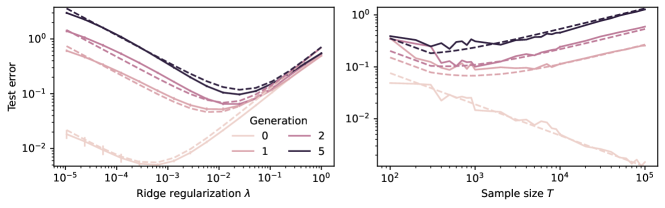
Figure 2: Demystifying model collapse in ridge regression (power-law covariance spectrum). The setup is: $d=300$, $\sigma=\sigma_{0}=1$, $\Sigma=\mathrm{diag}(\lambda_{1},\ldots,\lambda_{d})$, where $\lambda_{k}\propto k^{-2}$. Left plot corresponds to $T=10,000$ and Right plot corresponds to adaptive regularization $\lambda=T^{-\ell_{crit}}$, where $\lambda=\lambda(T)$ as proposed in Cui et al. (2022). See Section 6 for details. The broken curves are as predicted by our Theorem 5.2. Though the exponent $\ell=\ell_{crit}$ is optimal in classical case, it isn’t in the setup of model collapse. In fact here, the test error diverges with sample size $T$. Our theory proposes a corrected value of this exponent which gracefully adapts to synthesized data.

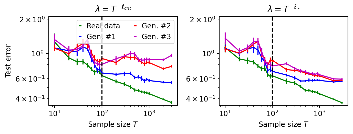
(a) RBF kernel (bandwidth = $10^{-4}$).

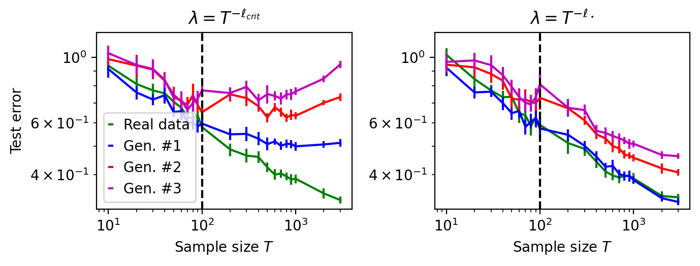
(b) Polynomial kernel (degree = $5$, bandwidth = $10^{-3}$).

Figure 3: Demystifying model collapse in kernel ridge regression on MNIST. with adaptive regularization $T^{-\ell}$ for different values of the exponent $\ell\geq 0$ (see Section 6 for full experimental setup). Top row: RBF kernel. Bottom row: polynomial kernel. In each plot, we show test error curves as a function of sample size $T$, from different generations ($n$) of fake data. The broken vertical line corresponds to $T=T_{0}$, where $T_{0}$ is the number of samples (from the true data distribution) which was used to train the label faker. The value of the exponent regularization $\ell=\ell_{\star}$ (broken curves) is the optimal value in the presence of iterative data relabeling, while $\ell=\ell_{crit}$ (solid curves) corresponds to the optimal value without iterative re-labelling (i.e $n=0$) proposed in Cui et al. (2022) (see (26)). Specifically, we take $\ell_{\star}=(b-a)\ell_{cirt}=b\ell_{crit}$, where $b=\log T_{0}/\log T$ (so that $T_{0}=T^{b}$), as proposed in Theorem 5.2, formula (29). Notice how the effect of fake data makes the test error become non decreasing in sample size $T$. This is effectively a collapse of the learned model.

Summary of Main Contributions.

Our main findings can be summarized as follows:

(1) Exact Characterization of Test Error. In Section 4 (Theorem 4.2), we obtain analytic formulae for test error under the influence of training data with fake / synthesized labels. For $n$-fold iteration of data-generation, this formula writes

$$E_{test}=E_{test}^{clean}+{\color[rgb]{1,0,0}n\times\Delta},$$ (1)

where $E_{test}^{clean}$ is the usual test error of the model trained on clean data (not AI-generated). The term $\Delta$ precisely highlights the effects of all the relevant problems parameters: feature covariance matrix, sample size, strength of data-generator, label noise level in clean data distribution, label noise level in fake data distribution, etc.

A direct consequence of this multiplicative degradation is that, over time (i.e as the number of generations becomes large), the effect of large language models (like ChatGPT) in the wild will be a pollution of the web to the extent that learning will be impossible. This will likely increase the value and cost of clean / non-AI-generated data.

(2) Modified Scaling Laws. In the case of power-law spectra, which is ubiquitous in machine learning Caponnetto & de Vito (2007); Spigler et al. (2020); Cui et al. (2022); Liang & Rakhlin (2020), we obtain in Section 5 (see Theorem 5.2) precise scaling laws which clearly highlight quantitatively the negative effect of training on fake data.

Further exploiting our analytic estimates, we obtain (Corollary 5.3) the optimal ridge regularization parameter as a function of all the problem parameters (sample size, spectral exponents, strength of fake data-generator, etc.). This new regularization parameter corresponds to a correction of the the value proposed in the classical theory on clean data Cui et al. (2022), and highlights a novel crossover phenomenon where for an appropriate tuning of the regularization parameter, the effect of training on fake data is a degradation of the fast error rate in the noiseless regime Cui et al. (2022); Caponnetto & de Vito (2007) to a much slower error rate which depends on the amount of true data on which the fake data-generator was trained in the first place. On the other hand, a choice of regularization which is optimal for the classical setting (training on real data), might lead to catastrophic failure: the test error diverges.

Apart from the above contributions, we modestly believe the arguments and techniques used to derive our results will find broader use in the community.

2 Review of Literature

Model Collapse.

Current LLMs Devlin et al. (2018); Liu et al. (2019); Brown et al. (2020); Touvron et al. (2023), including GPT-4 Achiam et al. (2023), were trained on predominantly human-generated text; similarly, diffusion models like DALL-E Ramesh et al. (2021), Stable Diffusion Rombach et al. (2022), Midjourney Midjourney (2023) are trained on web-scale image datasets. Their training corpora already potentially exhaust all the available clean data on the internet. A growing number of synthetic data generated with these increasingly popular models starts to populate the web, often indistinguishable from ”real” data. We have thus already raced into the future where our training corpora are irreversibly mixed with synthetic data and this situation stands to get worse. Recent works call attention to the potential dramatic deterioration in the resulting models, an effect referred to as ”model collapse” Shumailov et al. (2023). Several recent works demonstrate facets of this phenomenon empirically in various settings Hataya et al. (2023); Martínez et al. (2023a, b); Bohacek & Farid (2023); Briesch et al. (2023); Guo et al. (2023); Fan et al. (2023). Theoretically, a few works are emerging to analyze the effect of iterative training on self-generated (or mixed) data. Shumailov et al. (2023) attribute model collapse to two mechanisms: a finite sampling bias cutting off low-probability ”tails” and leading to more and more peaked distributions and function approximation errors, and analyze the (single) Gaussian case. In the context of vision models, Alemohammad et al. (2023) analyze ”self-consuming loops” by introducing a sampling bias that narrows the variance of the data at each generation, and provide theoretical analysis for the Gaussian model. Bertrand et al. (2023) explore scenarios involving a mix of clean data, representative of the true distribution, and synthesized data from previous iterations of the generator. Their analysis reveals that if the data mix consists exclusively of synthesized data, the generative process is likely to degenerate over time, leading to what they describe as a ’clueless generator’. Thus, the generator collapses: it progressively loses its ability to capture the essence of the data distribution it was intended to model. Conversely, they found that when the proportion of clean data in the mix is sufficiently high, the generator, under certain technical conditions, retains the capability to learn and accurately reflect the true data distribution. Note that such a compounding effect of synthesized data is already reminiscent of our decomposition (1).

Self-Distillation.

Importantly, the fake data generation process which is responsible for model collapse should not be confused with self-distillation as formulated in Mobahi et al. (2020) for example. Unlike model collapse, the data generation process in self-distillation actually helps performance of the downstream model. Indeed, self-distillation has control over the data generating process, which is carefully optimized for the next stage training. In the setting of model collapse, there is no control over the data generation process, since it constitutes synthesized data which typically comes from the wide web.

3 Theoretical Setup

We now present a setup which is simple enough to be analytically tractable, but rich enough to exhibit a wide range regimes for demystifying the phenomenon of model collapse (Shumailov et al., 2023; Hataya et al., 2023; Martínez et al., 2023a, b; Bohacek & Farid, 2023; Briesch et al., 2023; Guo et al., 2023) described in Section 1 and Section 2.

Notations. This manuscript will make use of the following standard notations. The set of integers from $1$ through $d$ is denoted $[d]$. Given a variable $z$ (which can be the input dimension $d$ or the sample size $T$, etc.) the notation $f(z)\lesssim g(z)$ means that $f(z)\leq Cg(z)$ for sufficiently large $z$ and an absolute constant $C$, while $f(z)\asymp g(z)$ means $f(z)\lesssim g(z)\lesssim f(z)$. For example, $1+z^{2}\asymp\max(1,z^{2})$. Further, $f(z)\simeq g(z)$ means $f(z)=(1+o(1))g(z)$, where $o(1)$ stands for a quantity which tends to zero in the limit $z\to\infty$. Finally, $\|u\|_{A}:=\sqrt{u^{\top}Au}$ defines the Mahalanobis norm induced by a positive-definite matrix $A$.

Data Distribution & Fake Data-Generation Process. Consider a distribution $P_{\Sigma,w_{0},\sigma^{2}}$ on $\mathbb{R}^{d}\times\mathbb{R}$ given by $(x,y)\sim P_{\Sigma,w_{0},\sigma^{2}}$ iff $\displaystyle\begin{split}\textbf{(Input) }x&\sim N(0,\Sigma),\\ \textbf{(Noise) }\epsilon&\sim N(0,\sigma^{2}),\text{ independent of }x,\\ \textbf{(Label) }y&=x^{\top}w_{0}+\epsilon.\end{split}$ (2) The positive integer $d$ is the input-dimension, the vector $w_{0}\in\mathbb{R}^{d}$ defines the ground-truth labelling function $x\mapsto x^{\top}w_{0}$, the matrix $\Sigma\in\mathbb{R}^{d\times d}$ captures the covariance structure of the input $x$. The scalar $\sigma^{2}$ is the level of label noise. Here, we consider linear models for clarity. We shall discuss kernel at the end of this section. So, in classical linear regression, we are given a sample $(X,Y)\equiv\{(x_{1},y_{1}),\ldots,(x_{T},y_{T})\}$ of size $T$ from $P_{\Sigma,w_{0},\sigma^{2}}$ and we seek a linear model $\widehat{w}^{pred}\in\mathbb{R}^{d}$ with small test error $E_{test}(\widehat{w}^{pred})$, defined by

$$\begin{split}E_{test}(\widehat{w}^{pred})&:=\mathbb{E}_{X,Y}\,\mathbb{E}_{x,y}[(x^{\top}\widehat{w}^{pred}-y)^{2}]-\sigma^{2}\\ &=\mathbb{E}_{X,Y}[\|\widehat{w}^{pred}-w_{0}\|_{\Sigma}^{2}],\end{split}$$ (3)

where $(x,y)\sim P_{\Sigma,w_{0},\sigma^{2}}$ is a random clean test point.

In our setup for studying model collapse, the design matrix $X\in\mathbb{R}^{T\times d}$ stays the same, but the vector of labels $Y\in\mathbb{R}^{n}$ is generated by an iterative relabelling process, where each generation of the model serves as the labeller for the data for the next generation. This process is described below. Building the Fake / Synthesized Data Generator. $\displaystyle P_{\Sigma,\widehat{w}_{0},\sigma^{2}}\to P_{\Sigma,\widehat{w}_{1},\sigma_{0}^{2}}\to\ldots\to P_{\Sigma,\widehat{w}_{n},\sigma_{0}^{2}},$ (4) where $n\in\mathbb{N}$ is the number of generations and – For $n=0$, we take $\widehat{w}_{0}:=w_{0}$ (the true data labelling function). This corresponds to generating $T_{0}$ from the true data distribution $P_{\Sigma,w_{0},\sigma^{2}}$. – For any $m\in\{1,2,\ldots n\}$, the fake data labelling function $\widehat{w}_{m}$ is OLS fitted on an iid dataset $\mathcal{D}_{m-1}$ of size $T_{0}$ from $P_{\Sigma,\widehat{w}_{m-1},\sigma_{0}^{2}}$. In vector form: • $X_{m-1}\sim N(0,\Sigma)^{\otimes T_{0}}$, $E_{m-1}\sim N(0,\sigma_{0}^{2}I_{T_{0}})$, • $\widehat{Y}_{m-1}=X_{m-1}\widehat{w}_{m-1}+E_{m-1}$, • $\widehat{w}_{m}=X_{m-1}^{\dagger}\widehat{Y}_{m-1}$ (OLS), where $X_{m-1}$ and $E_{m-1}$ are independent, and also independent of all previous generations. The motivation for OLS (ordinary least-squares) in defining the $\widehat{w}_{m}$’s is just for analytical tractability. The above process is completely determined by the triplet $(n,T_{0},\sigma_{0}^{2})$. We don’t require $\sigma_{0}^{2}=\sigma^{2}$. Note that the distribution of the covariates stays the same all through the above process; only the conditional distribution of the labels is changed.

Remark 3.1.

Without loss of generality, we could consider different values of $(T_{0},\sigma_{0}^{2})$ for each generation, but we use the same value everywhere for simplicity of presentation.

The mental picture is as follows: each generation $\widehat{w}_{n}$ can be seen as a proxy for a specific version of ChatGPT, for example. The sample size $T_{0}$ used to create the fake labelling functions $\widehat{w}_{n}$ is a proxy for the strength of the fake data-generator thus constructed. Other works which have considered model collapse under such a self-looping training process include (Shumailov et al., 2023; Alemohammad et al., 2023; Bertrand et al., 2023).

Finally, note that this setup is not self-distillation (as defined in Mobahi et al. (2020) for example), as the downstream model has no control whatsoever on the generation of the synthetic / fake labels.

The Downstream Model: Ridge Regression. For a regularization parameter $\lambda\geq 0$, let $\widehat{w}_{n}^{pred}=\widehat{w}^{pred}_{n,T_{0},\sigma_{0}^{2},T,\lambda}\in\mathbb{R}^{d}$ be the ridge predictor constructed from and iid sample $\{(x_{1},y_{1}),\ldots,(x_{T},y_{T})\}$ of size $T$ from the $n$-fold fake data distribution $P_{\Sigma,\widehat{w}_{n},\sigma_{0}^{2}}$ given in (4), i.e $\displaystyle\widehat{w}_{n}^{pred}=\begin{cases}X^{\dagger}Y,&\mbox{ if }\lambda=0,\\ (\widehat{\Sigma}+\lambda I_{d})^{-1}X^{\top}Y/T,&\mbox{ otherwise,}\end{cases}$ (5) where $X=(x_{1},\ldots,x_{T})\in\mathbb{R}^{T\times d}$ is the design matrix, $X^{\dagger}$ is its Moore-Penrose pseudo-inverse, $Y:=(y_{1},\ldots,y_{T})\in\mathbb{R}^{T}$ is the vector of labels, and $\widehat{\Sigma}:=X^{\top}X/T\in\mathbb{R}^{d\times d}$ is the sample covariance matrix.

We are interested in the dynamics of the test error $E_{test}(\widehat{w}^{pred}_{n})$ (according to formula (3)) of this linear model. Note that the evaluation of the model is done on the true data distribution $P_{\Sigma,w_{0},\sigma^{2}}$, even though the model is trained on fake data distribution $P_{\Sigma,\widehat{w}_{n},\sigma_{0}^{2}}$. Also note that for $n=0$, $E_{test}^{clean}:=E_{test}(\widehat{w}_{0}^{pred})$ corresponds to the usual test error when the downstream model is trained on clean data.

A Note on Extension to Kernel Methods. Though we present our results in the case of linear regression in $\mathbb{R}^{d}$ for clarity, they can be rewritten in equivalent form in the kernel setting. Indeed, like in (Caponnetto & de Vito, 2007; Simon et al., 2021; Cui et al., 2022; Wei et al., 2022), it suffices to replace $x$ with a feature map induced by a kernel $K$, namely $\psi(x):=K_{x}\in\mathcal{H}_{K}$. Here, $\mathcal{H}_{K}$ is the reproducing kernel Hilbert space (RKHS) induced by $K$. In the data distribution (2), we must now replace the Gaussian marginal distribution condition $x\sim N(0,\Sigma)$ with $\psi(x)\sim N(0,\Sigma)$. The ground-truth labeling linear function in (2) is now a just a general function $f_{0}\in L^{2}(P_{x})$. The ridge predictor (5) is then given by (Representer Theorem) $\widehat{f}_{n}^{pred}(x):=K(X,x)^{\top}\widehat{c}_{n}$, with $\widehat{c}_{n}=(G+\lambda TI_{n})^{-1}Y\in\mathbb{R}^{n}$, where $K(X):=(K_{x_{1}},\ldots,K_{x_{T}})$, and $G=K(X)K(X)^{\top}=(K(x_{i},x_{j}))_{1\leq i,j\leq T}\in\mathbb{R}^{n\times n}$ is the Gram matrix.

4 Exact Test Error Characterization

In this section we establish generic analytic formulae for the test error of the downstream model $\widehat{w}_{n}^{pred}$ (5) trained on $n$-fold fake data-generation as outlined in Section 3.

4.1 Warm-up: Unregularized Downstream Model

For a start, let us first consider the case of ridgeless regression (corresponding to $\lambda=0$ in Equation (5)).

Theorem 4.1.

For an $n$-fold fake data generation process with $T_{0}\geq d+2$ samples, the test error for the linear predictor $\widehat{w}_{n}^{pred}$ given in (5) learned on $T\geq d+2$ samples, with $\lambda=0$, is given for $T\to\infty$ by

$$E_{test}(\widehat{w}_{n}^{pred})\simeq\frac{\sigma^{2}\phi}{1-\phi}+{\color[rgb]{1,0,0}\frac{n\sigma_{0}^{2}\phi_{0}}{1-\phi_{0}}},\,\phi=\frac{d}{T},\phi_{0}=\frac{d}{T_{0}}.$$ (6)

The first term $E_{test}(\widehat{w}_{0}^{pred})\simeq\sigma^{2}\phi/(1-\phi)$ in (6) corresponds the to the usual error when the downstream model is fitted on clean data (see Hastie et al. (2022), for example). The additional term $n\sigma_{0}^{2}\phi_{0}/(1-\phi_{0})$, proportional to the number of generations $n$ is responsible for model collapse.

Low-Dimensional Regime.

In the low-dimensional problems (fixed $d$), Theorem 4.1 already predicts a change of scaling law from $E_{test}(\widehat{w}_{0}^{pred})\asymp\sigma^{2}T^{-1}$ to $E_{test}(\widehat{w}_{n}^{pred})\asymp\sigma^{2}T^{-1}+n\sigma_{0}^{2}T_{0}^{-1}$. Thus, as the sample size $T$ is scaled up, the test error eventually plateaus and doesn’t vanish. This phenomenon is clearly visible in Figure 1. In section 5, we shall establish a similar picture in a high-dimensional regime.

Regularize ?

Note that the test error of the null predictor $w_{null}=0$ is $E_{test}(w_{null})=\|w_{0}\|_{\Sigma}^{2}$, and so

$$\frac{E_{test}(\widehat{w}_{n}^{pred})}{E_{test}(w_{null})}=\frac{1}{\text{SNR}}\frac{\phi}{1-\phi}+\frac{n}{\text{SNR}_{0}}\frac{\phi_{0}}{1-\phi_{0}},$$ (7)

where $\text{SNR}:=\|w_{0}\|_{\Sigma}^{2}/\sigma^{2}$ and $\text{SNR}_{0}:=\|w_{0}\|_{\Sigma}^{2}/\sigma_{0}^{2}$. We deduce that if $n\gg\mathrm{SNR}_{0}/(1/\phi_{0}-1)$, then the learned model is already much worse than the null predictor! This suggests that a good strategy for mitigating the negative effects on learning on AI-generated data is regularization at an appropriate level, as illustrated in Figure 3.

4.2 Main Result I: A General Formula for Test Error

We now consider the case of general ridge penalty $\lambda>0$, and drop the requirement $T\geq d+2$. We still make the simplifying assumption that $T_{0}\geq d+2$, i.e each generation of the fake data-generator is based on enough examples from the previous generation.

Theorem 4.2.

For an $n$-fold fake data generation process with $T_{0}\geq d+2$, the test error of a ridge predictor $\widehat{w}_{n}^{pred}$ based on a fake sample of size $T\geq 1$ with regularization parameter $\lambda>0$ is given by

$$E_{test}(\widehat{w}_{n}^{pred})=E_{test}(\widehat{w}_{0}^{pred})+{\color[rgb]{1,0,0}n\sigma_{0}^{2}\rho},$$ (8)

$$\quad\rho:=\frac{\mathbb{E}\,\mathrm{tr}(\Sigma^{-1}\widehat{\Sigma}(\widehat{\Sigma}+\lambda I_{d})^{-1}\Sigma(\widehat{\Sigma}+\lambda I_{d})^{-1}\widehat{\Sigma})}{T_{0}-d}.$$ (9)

Note that $E_{test}(\widehat{w}_{0}^{pred})=Bias+Var$ given in (16), (17) is the usual test error for ridge regression on non-fake data.

In particular, in the ridgeless case where $T\geq d+2$ and $\lambda=0$, it holds that $\rho=\phi_{0}/(1-\phi_{0})$ where $\phi_{0}:=d/T_{0}$ is the the level of ”parametrization” of the fake data generator.

As said in the theorem, the term $E_{test}(\widehat{w}_{0}^{pred})$ corresponds to the usual test error when the predictor is learned on real (not fake) data, for which well-known formulae exist in a variety of scenarios (see Proposition 4.4). What is new is the term in red, $n\sigma_{0}^{2}\rho$, where $n$ is the number of generations. This result is of the promised form (1), with $\Delta=\sigma_{0}^{2}\rho$. The additional term $n\sigma_{0}^{2}\rho$ induced by the fake labeling process is in competition with the usual test error $E_{test}(\widehat{w}_{0}^{pred})$. Understanding the interaction of these two terms is key to demystifying the origins of model collapse.

Importantly, the term $\rho$ only depends on the design matrix $X$ and the covariance matrix $\Sigma$. In an appropriate asymptotic regime, it will only depend on: $T$, $d$, and the spectral properties of $\Sigma$. Observe that we always have $\rho\leq d/(T_{0}-d)$, a consequence of the fact that all the eigenvalues of the positive-definite matrix $(\widehat{\Sigma}+\lambda I_{d})^{-1}\widehat{\Sigma}$ are at most $1$. Moreover, $\rho\to 0$ in the limit $\lambda\to\infty$ (corresponding to the null predictor). The precise analysis of this term will be carried out via random matrix theory (RMT) tools.

4.3 Essential Random Matrix Theory

In order to analyze the tracial term $\rho$ appearing in (9) and ultimately obtain analytic insights on the dynamics of $E_{test}(\widehat{w}_{n}^{pred})$, we need some tools from RMT. Such tools have been used extensively to analyze ridge regression (Richards et al., 2021; Hastie et al., 2022; Bach, 2023).

Degrees of Freedom and Random Matrix Equivalents. Define, for any $\lambda\geq 0$ and $m\in\mathbb{N}_{\star}$, the $m$th order ”degrees of freedom” of the covariance matrix $\Sigma$, by

$$\mathrm{df}_{m}(\Sigma;\lambda)=\mathrm{df}_{m}(\lambda):=\mathrm{tr}((\Sigma+\lambda I_{d})^{-m}\Sigma^{m}).$$ (10)

Note that $\mathrm{df}_{m}(\lambda)\leq d$ always. Finally, define an increasing function $\lambda\mapsto\kappa(\lambda,T)$ on $\mathbb{R}_{+}$ implicitly by

$$\begin{split}\kappa(\lambda,T)-\lambda&=\kappa(\lambda,T)\cdot\mathrm{df}_{1}(\kappa(\lambda,T))/T.\end{split}$$ (11)

The effect of ridge regularization at level $\lambda\geq 0$ is to improve the conditioning of the empirical covariance matrix $\widehat{\Sigma}$, what the $\kappa$-function does is translate this into regularization on $\Sigma$ at a higher level $\kappa(\lambda,T)\geq\lambda$, which reduces the ”capacity” of the latter, i.e the ”effective dimension” of the underlying problem. Quantitatively, there is an equivalence of the form $\mathrm{df}_{1}(\widehat{\Sigma};\lambda)\approx\mathrm{df}_{1}(\Sigma;\kappa(\lambda,T)).$ Roughly speaking, RMT is the business of formalizing such relationships.

Example: Isotropic Covariance. For example, note that $\mathrm{df}_{m}(t)\equiv d/(1+t)^{m}$ (polynomial decay) in the isotropic case where $\Sigma=I_{d}$. Consequently, we have $\kappa(\lambda,T)-\lambda=(d/T)\kappa(\lambda,T)/(1+\kappa(\lambda,T))$. With $\phi=d/T$ and $\overline{\phi}:=1-\phi$, it is then easy to obtain the following well-known formula

$$\kappa(\lambda,T)=\frac{1}{2}\left(\lambda-\overline{\phi}+\sqrt{(\lambda-\overline{\phi})^{2}+4\lambda}\right).$$ (12)

which is reminiscent of the celebrated Marchenko-Pastur law (Marčenko & Pastur, 1967; Bai & Silverstein, 2010).

High-Dimensional Regimes. We will temporarily work under the following standard assumption

Assumption 4.3.

$\Sigma=\Sigma_{d}$ (i.e a sequence of covariance matrix indexed by the dimensionality $d$) has spectrum bounded away from $0$ uniformly w.r.t $d$. Moreover, the empirical spectral distribution $\sum_{j=1}^{d}\delta_{\lambda_{j}}$ of $\Sigma$ converges in the limit $d\to\infty$, to a compactly-supported distribution $\mu$ on $\mathbb{R}^{+}$.

Furthermore, we shall work in the following so-called proportionate asymptotic scaling which is standard in analyses based on RMT

$$T,d\to\infty,\quad d/T\to\phi\in(0,\infty).$$ (13)

Later in Section 5 when we consider power-law spectra, this scaling will be extended to account for more realistic case where $d$ and $T$ are allowed to be polynomial in one order, Polynomial Scaling Regime. $\displaystyle T,d\to\infty,\quad d^{1/C}\lesssim T\lesssim d^{C},$ (14) for some absolute constant $C\geq 1$. RMT in such non-proportionate settings are covered by the theory developed in (Knowles & Yin, 2017; Wei et al., 2022).

Bias-Variance Decomposition. With everything now in place, let us recall for later use, the following classical bias-variance decomposition for ridge regression (for example, see Richards et al. (2021); Hastie et al. (2022); Bach (2023))

Proposition 4.4.

Under Assumption 4.3, in the limit (13) the test error of a ridge predictor $w(\lambda)$ based on $T$ iid samples from the true data distribution $P_{\Sigma,w_{0},\sigma^{2}}$ is given by

$$E_{test}(w(\lambda)) =\mathbb{E}\,\|w(\lambda)-w_{0}\|_{\Sigma}^{2}\simeq Bias+Var,$$ (15)

$$Bias \simeq\frac{\kappa^{2}w_{0}^{\top}\Sigma(\Sigma+\kappa I)^{-2}w_{0}}{{1-\mathrm{df}_{2}(\kappa)/T}},$$ (16)

$$Var \simeq\frac{\sigma^{2}\mathrm{df}_{2}(\kappa)}{T}\cdot\frac{1}{1-\mathrm{df}_{2}(\kappa)/T},$$ (17)

where $\kappa=\kappa(\lambda,T)$ is as given in (11).

In particular, in the isotropic case where $\Sigma=I_{d}$, we have

$$E_{test}(w(\lambda))\simeq\frac{\kappa^{2}\|w_{0}\|_{2}^{2}+\sigma^{2}\phi}{(1+\kappa)^{2}-\phi}.$$ (18)

Note that (Wei et al., 2022) has established a version of this result in the polynomial scaling regime (14).

4.4 Main Result II: Analytic Formula for Test Error

The following result which generalizes Theorem 4.1 gives the test error for the downstream ridge model $\widehat{w}_{n}^{pred}$ define in (5), in the contest of fake training data, and will be exploited later to obtain precise estimates in different regimes.

Theorem 4.5.

Suppose Assumption 4.3 is in order. For an $n$-fold fake data-generation process, the test error of a downstream model $\widehat{w}_{n}^{pred}$ based on a fake sample of size $T$ with ridge regularization $\lambda$ is given in the limit (13) by

$$E_{test}(\widehat{w}_{n}^{pred})\simeq Bias+Var+{n\sigma_{0}^{2}\rho},$$ (19)

where $Bias$ and $Var$ are as given in (16), (17), and

$$\begin{split}\rho&\simeq\frac{\mathrm{df}_{2}(\kappa)}{T_{0}-d}+\frac{\kappa^{2}\mathrm{tr}\left(\Sigma+\kappa I_{d}\right)^{-2}}{T_{0}-d}\cdot\frac{\mathrm{df}_{2}(\kappa)}{T-\mathrm{df}_{2}(\kappa)},\end{split}$$ (20)

with $\kappa=\kappa(\lambda,T)$ is as given in (11).

In the special case of isotropic features ($\Sigma=I_{d})$,

$$\rho\simeq\frac{\phi_{0}}{1-\phi_{0}}\left(\frac{1}{(1+\kappa)^{2}}+\frac{1}{(1+\kappa)^{2}}\frac{\phi\kappa^{2}}{(1+\kappa)^{2}-\phi}\right),$$ (21)

where $\phi_{0}:=d/T_{0}$ and $\kappa=\kappa(\lambda)$ is as given in (12).

Such a result, empirically illustrated in Figures 1 and 2, gives us the needed anaytical handle for understanding $n$-fold model collapse in terms of all relevant problem hyper-parameters: spectral properties of covariance matrix $\Sigma$, regularization level $\lambda$, label-noise level $\sigma^{2}$, etc.

5 The Case of Heavy Tails (Power Law)

Now, consider a variant of the distribution (2), in the setting considered in (Caponnetto & de Vito, 2007; Richards et al., 2021; Simon et al., 2021; Cui et al., 2022), for $d\to\infty$. Let

$$\Sigma=\lambda_{1}v_{1}v_{1}^{\top}+\ldots+\lambda_{d}v_{d}v_{d}^{\top}$$ (22)

be the spectral decomposition of the covariance matrix $\Sigma$, with eigenvalues with $\lambda_{1}\geq\ldots\geq\lambda_{d}\geq 0$ and eigenvectors $v_{1},\ldots,v_{d}\in\mathbb{R}^{d}$. Define coefficients $c_{j}:=w_{0}^{\top}v_{j}$, i.e the projection of $w_{0}$ along the $j$th eigendirection of $\Sigma$.

We shall work under the following spectral conditions

$$\begin{split}&\textbf{(Capacity Condition) }\lambda_{j}\asymp j^{-\beta}\text{ for all }j\in[d],\\ &\textbf{(Source Condition) }\|\Sigma^{1/2-r}w_{0}\|=O(1),\end{split}$$ (23)

where $\beta>1$ and $r\geq 0$. The parameter $r$ measures the amount of dispersion of $w_{0}$ relative to the spectrum of $\Sigma$; a large value of $r$ means $w_{0}$ is concentrated only along a few important eigendirections directions (i.e the learning problem is easy). For later convenience, define $\underline{r}$ and $\delta$ by

$$\underline{r}:=\min(r,1),\quad\delta:=1+\beta(2r-1).$$ (24)

As noted in (Cui et al., 2022), the above source condition is satisfied if $c_{j}\asymp j^{-\delta/2}$ for all $j\in[d]$.

As in (Cui et al., 2022), consider adaptive ridge regularization strength of the form

$$\lambda=\lambda(T)\asymp T^{-\ell},$$ (25)

for fixed $\ell\geq 0$. The case where $\ell=0$ corresponds to non-adaptive regularization; otherwise, the level of regularization decays polynomially with the sample size $T$. Define

$$\ell_{crit}:=\beta/(1+2\beta\underline{r}),$$ (26)

In (Cui et al., 2022) KRR under norm circumstances (corresponding to $n=0$, i.e no fake data) was considered and it was shown that this value for the regularization exponent in (25) is minimax-optimal for normal test error in the noisy regime, namely $E_{test}(\widehat{w}_{0}^{pred})\asymp T^{-c}$, where

$$c:=\frac{2\beta\underline{r}}{2\beta\underline{r}+1}\in(0,1).$$ (27)

This represents a crossover from the noiseless regime where it was shown that the test error scales like $E_{test}(\widehat{w}_{0}^{pred})\asymp T^{-2\beta\underline{r}}$, a must faster rate. We shall show that the picture drastically changes in the context of training on fake data considered in this manuscript for the purpose of understanding model collapse (Shumailov et al., 2023).

Remark 5.1.

Unlike (Cui et al., 2022) which considered the proportionate scaling limit (13) for input dimension $d$ and sample size $T$, we shall consider the more general (and more realistic) polynomial scaling limit (14), and invoked the tools of so-called anisotropic local RMT developed in (Knowles & Yin, 2017) to compute deterministic equivalents for quantities involving the spectra of random matrices.

5.1 Main Result III: A ”Collapsed” Scaling Law

The following result shows that model collapse is a modification of usual scaling laws induced by fake data.

Theorem 5.2.

Consider $n$-fold fake-data generation with sample size $T_{0}\geq d+2$ and set $\phi_{0}:=d/T_{0}\in(0,1)$. For a ridge predictor $\widehat{w}_{n}^{pred}$ given in (5) based on a fake sample of size $T$, with regularization parameter $\lambda=\lambda(T)$ tuned adaptively as in (25) with exponent $\ell\in[0,\beta]$, the test error satisfies the following scaling law in the limit (14)

$$\begin{split}&E_{test}(\widehat{w}_{n}^{pred})\asymp\max(\sigma^{2},T^{1-2\underline{r}\ell-\ell/\beta)})\cdot T^{-(1-\ell/\beta)}\\ &\quad\quad+{\color[rgb]{1,0,0}n\frac{\sigma_{0}^{2}}{1-\phi_{0}}\max\left(T/T_{0},\phi_{0}\right)\cdot T^{-(1-\ell/\beta)}}.\end{split}$$ (28)

5.2 Optimal Regularization for Mitigating Collapse

Let us provide an instructive interpretation of the result.

Noiseless Regime. Suppose $\sigma=0$ (or equivalently, exponentially small in $T$) and $\phi_{0}\in(0,1)$ is fixed, and consider a number of generations $n$ such that $n\sigma_{0}^{2}\asymp T^{a}$, where $0\leq a\leq 1-\ell/\beta\leq 1$. Note that $a=0$ corresponds to constant number of generations. Also take $T_{0}=T^{b}$, for some constant $b\in(0,\infty)$. According to Theorem 5.2, if we want to balance out the model-collapsing negative effect of training on fake data, we should chose $\ell$ so as to balance the second term $n(T/T_{0})T^{-(1-\ell/\beta)}=T^{-(b-\ell/\beta-a)}$ and the first term $T^{-2\ell\underline{r}}$ in (28). This gives the following result.

Corollary 5.3.

In the setting of Theorem 5.2 with $T_{0}\asymp T^{b}$ and $n\asymp T^{b}$, the optimal exponent of the ridge regularization parameter in (25) is $\ell=\ell_{\star}$, where

$$\ell_{\star}=\min((b-a)\ell_{crit},\beta),$$ (29)

and $\ell_{crit}$ is as in (26), with corresponding optimal test error

$$\inf_{\ell\geq 0}E_{test}(\widehat{w}_{n}^{pred})\asymp E_{test}(\widehat{w}_{n}^{pred})\big{|}_{\ell=\ell_{\star}}\asymp T^{-(b-a)c}.$$

Observe that when $(b-a)c<2\beta\underline{r}$, which is the case when $n=O(1)$, $r\geq 1$ and $b\leq a+1$, this corresponds to the condition $T\gtrsim T_{0}$), the above result represents a crossover from the fast rate $E_{test}(\widehat{w}_{0}^{pred})\asymp T^{-2\beta\underline{r}}$ in the case of training on clean data (Cui et al., 2022), to a much slower rate $E_{test}(\widehat{w}_{n}^{pred})\asymp T^{-(b-a)c}$, attained by the adaptive regularization $\lambda\asymp T^{-\ell_{\star}}$, which is optimal in this setting. Furthermore, in this setting if we still use $\lambda\asymp T^{-\ell_{crit}}$ as proposed in (Cui et al., 2022) in the clean data setting, Corollary 5.3 predicts that $E_{test}(\widehat{w}_{n}^{pred})\gtrsim T^{-(b-\ell_{crit}/\beta-a)}=T^{-(c+b-a-1)},$ which diverges to infinity if $b\geq a+1-c$. This is a catastrophic form of model collapse, and is empirically illustrated in Figures 2 and 3.

Noisy Regime. Now fix $\sigma^{2}\neq 0$ and $\phi_{0}\in(0,1)$. In this regime, Theorem 5.2 predicts that consistency (i.e $E_{test}(\widehat{w}_{n}^{pred})\overset{T\to\infty}{\longrightarrow}0$) is only possible if $\ell\leq\ell_{\star}$. First consider values of $\ell$ for which the variance is smaller than the bias, i.e $0\leq\ell\leq\ell_{crit}$. We get $E_{test}(\widehat{w}_{n}^{pred})\asymp T^{-2\ell\underline{r}}+T^{-(b-a-\ell/\beta)},$ which is minimized by taking $\ell=\min(\ell_{\star},\ell_{crit})$. For other values of $\ell$, the variance dominates and we have

$$E_{test}(\widehat{w}_{n}^{pred})\asymp T^{-(1-\ell/\beta)}+T^{-(b-\ell/\beta-a)}\asymp T^{-(\gamma-\ell/\beta)},$$

where $\gamma:=\min(1,b-a)$. This is minimized by taking $\ell=\ell_{crit}$, leading to $E_{test}(\widehat{w}_{n}^{pred})\asymp T^{-(\gamma-1/(2\beta\underline{r}+1))}$. This tends to zero with $T\to\infty$ only if $b>a+1/(2\beta\underline{r}+1)$.

6 Experiments

We run a couple of experiments on both simulated and real data to empirically validate our theoretical results.

Simulated Data. We consider ordinary / linear ridge regression in $\mathbb{R}^{d}$, for $d=300$ and different structures for the covariance matrix $\Sigma$ of the inputs: isotropic (i.e $\Sigma=I_{d}$) and power-law (23), with $(\beta,r)=(2,0.375)$. For each value of $n$ (the generation index), the fake data-generator is constructed according to the process described in (4), with $\sigma=0.1$ and $\sigma_{0}=0.2$ (results are similar for other nonzero values of $\sigma$ and $\sigma_{0}$). Then, for different values of $T$ (between $1$ and $1000,000$), a sample of size $T$ is drawn from this fake data-generator and then a downstream ridge model (5) is fitted. The test set consists of $100,000$ clean pairs $(x,y)$ form the true data distribution $P_{\Sigma,w_{0},\sigma^{2}}$. This experiment is repeated $10$ times to generate error bars. The results for the isotropic setting are shown in Figure 1 and the results for the power-law setting are shown in Figure 2.

Real Data: Kernel Ridge Regression on MNIST. As in (Cui et al., 2022; Wei et al., 2022) we consider a distribution on MNIST, a popular dataset in the ML community. Classification dataset normally contains $60,000$ training and $10,000$ test data points (handwritten), with labels from 0 to 9 inclusive. Like in (Cui et al., 2022), we convert the labels into real numbers (i.e a regression problem) like so: $y=\text{label}\text{ mod }2+\text{ noise }$, where the variance of the noise is $\sigma^{2}=1$ (for simplicity, we also set $\sigma_{0}^{2}=1$). The test set consists of $10,000$ pairs $(x,y)$, with the labels $y$ constructed as described in previous sentence. The fake data used for training is generated as in the previous experiment, but via kernel ridge regression (instead of least squares) with polynomial kernel (degree = $5$, bandwidth = $10^{-4}$) and polynomial kernel (degree = $5$). Note that it was empirically shown in (Cui et al., 2022) that these datasets verify (23) with $(\beta,r)\approx(1.65,0.097)$ in the case of the aforementioned RBF kernel, and $(\beta,r)\approx(1.2,0.15)$ in the case of the polynomial kernel. Then, for different values of $T$ (between $1$ and $1000$), a sample of size $T$ is drawn from the the this fake data-generator and then a downstream kernel ridge model is fitted. Each of these experiments are repeated $10$ times to generate error bars (due to different realizations of label noise). The results are shown in Figure 3.

7 Concluding Remarks

As we navigate the ”synthetic data age”, our findings signal a departure from traditional test error rates (e.g neural scaling laws), introducing novel challenges and phenomena with the integration of synthetic data from preceding AI models into training sets. Our work provides a solid analytical handle for demystifying the model collapse phenomenon as a modification of usual scaling laws caused by fake / synthesized training data.

On the practical side, our analysis reveals that AI-generated data alters the optimal regularization for downstream models. Drawing from the insight that regularization mirrors early stopping Ali et al. (2019), our study suggests that models trained on mixed real and AI-generated data may initially improve but later decline in performance (model collapse), necessitating early detection of this inflection point. This observation prompts a re-evaluation of current training approaches and underscores the complexity of model optimization in the era of synthetic data.

8 Acknowledgements

YF and JK acknowledge support through NSF NRT training grant award 1922658. Discussions with Bruno Loureiro are gratefully acknowledged. This work was supported in part through the NYU IT High Performance Computing resources, services, and staff expertise.

Appendix A Exact Characterization of Test Error Under Model Collapse

A.1 Proof of Theorem 4.1 (Rigeless Regression / OLS)

For $n=0$, we have

$$\begin{split}E_{test}(\widehat{w}_{0}^{pred})&=\mathbb{E}\,\|\widehat{w}_{0}^{pred}-w_{0}\|^{2}_{\Sigma}=\mathbb{E}\|(X_{0}^{\top}X_{0})^{-1}X_{0}^{\top}E_{n-1}\|^{2}_{\Sigma}\\ &=\sigma^{2}\mathbb{E}\mathrm{tr}((X_{0}^{\top}X_{0})^{-1}\Sigma)=\sigma^{2}\frac{d}{T-d-1}\simeq\frac{\sigma^{2}\phi}{1-\phi},\end{split}$$ (30)

where $\phi:=d/T\in(0,1)$ and we have used Lemma A.1 in the last step. This is a well-known result for the test error of linear regression in the under-parametrized regime, without any AI pollution (fake / synthesize training data).

Analogously, for $n=1$ one computes the test error after the first generation of fake data as follows

$$\begin{split}E_{test}(\widehat{w}_{1}^{pred})&=\mathbb{E}\|\widehat{w}_{1}^{pred}-w_{0}\|^{2}_{\Sigma}=\mathbb{E}\|\widehat{w}_{1}^{pred}-\widehat{w}_{1}+\widehat{w}_{1}-\widehat{w}_{0}\|^{2}_{\Sigma}\\ &=\mathbb{E}\|(X_{0}^{\top}X_{0})^{-1}X_{0}E_{0}+\widehat{w}_{0}^{pred}-w_{0}\|^{2}_{\Sigma}=\mathbb{E}\,\|w_{0}-\widehat{w}_{0}^{pred}\|^{2}_{\Sigma}+\mathbb{E}\,\|(X_{0}^{\top}X_{0})^{-1}X_{0}^{\top}E_{0}\|^{2}_{\Sigma}\\ &=E_{test}(\widehat{w}_{0}^{pred})+\frac{\sigma_{0}^{2}d}{T_{0}-d-1}\simeq\frac{\sigma^{2}\phi}{1-\phi}+\frac{\sigma_{0}^{2}\phi_{0}}{1-\phi_{0}},\end{split}$$

where $\phi_{0}=d/T_{0}\in(0,1)$. Continuing the induction on $n$, we obtain the result. ∎

A.2 Proof of Theorem 4.2 (Ridge Regression)

The case $n=0$ tautological. The proof for the cases $n\geq 1$ is by induction. Let $X$ a random $T\times d$ matrix from $N(0,\Sigma)$ and let $E$ be a $T$-dimensional Gaussian vector independent of $X$, with iid entries from $N(0,\sigma^{2})$. The final predictor fitted on the $n$ generation of fake data is $\widehat{w}_{n}^{pred}=RX^{\top}Y/T$, where $S=\widehat{\Sigma}:=X^{\top}X/T$, $R=(S+\lambda I_{d})^{-1}$, and $Y=X\widehat{w}_{n}+E$, where

$$\begin{split}\widehat{w}_{n}&:=X_{n-1}^{\dagger}\widehat{Y}_{n-1}=X_{n-1}^{\dagger}(X_{n-1}\widehat{w}_{n-1}+E_{n-1}).\\ \end{split}$$ (31)

Thus, we have

$$\widehat{w}_{n}^{pred}=RX^{\top}Y/T=RSP_{n-1}\widehat{w}_{n-1}+RSX_{n-1}^{\dagger}E_{n-1}+RX^{\top}E/T,$$

where $P_{n-1}:=X_{n-1}^{\dagger}X_{n-1}$ is the orthogonal projector unto the subspace of $\mathbb{R}^{d}$ spanned by the rows of $X_{n-1}$.

Since $X_{n-1}$ has full column rank (which happens w.p $1$ if $T_{0}\geq d+2$), then $X_{n-1}^{\dagger}=(X_{n-1}^{\top}X_{n-1})^{-1}X_{n-1}^{\top}$, $P_{n-1}=I_{d}$, and the above further simplifies to

$$\widehat{w}_{n}^{pred}=RS\widehat{w}_{n-1}+RX^{\top}E/T+RS(X_{n-1}^{\top}X_{n-1})^{-1}X_{n-1}^{\top}E_{n-1}\overset{D}{=}\widehat{w}_{n-1}^{pred}+\Delta_{n},$$

where $\Delta_{n}:=RS(X_{0}^{\top}X_{0})^{-1}X_{0}^{\top}E_{n-1}$. Since $\widehat{w}_{n-1}$ and $\Delta_{n}$ are independent by construction, we deduce that

$$E_{test}(\widehat{w}_{n}^{pred})=\mathbb{E}\,\|\widehat{w}_{n}^{pred}-w_{0}\|_{\Sigma}^{2}=\mathbb{E}\,\|\widehat{w}_{n-1}^{pred}-w_{0}\|_{\Sigma}^{2}+\mathbb{E}\,\|\Delta_{n}\|_{\Sigma}^{2}.$$ (32)

The first term on the RHS is just $E_{test}(\widehat{w}_{n-1}^{pred})$. Since $E_{n-1}$ is a $T_{0}$-dimensional Gaussian vector with iid entries from $N(0,\sigma_{0}^{2})$, the second term evaluates to

$$\begin{split}\mathbb{E}\,\|\Delta_{n}\|_{\Sigma}^{2}&=\mathbb{E}\,\|RSX_{0}^{\dagger}E_{n-1}\|_{\Sigma}^{2}\\ &=\sigma_{0}^{2}\mathbb{E}\,\mathrm{tr}(X_{0}(X_{0}^{\top}X_{0})^{-1}SR\Sigma RS(X_{0}^{\top}X_{0})^{-1}X_{0}^{\top}),\text{ taking expectations w.r.t }E_{n-1}\\ &=\sigma_{0}^{2}\mathbb{E}\,\mathrm{tr}((X_{0}^{\top}X_{0})^{-1}SR\Sigma RS),\text{ by cyclic property of trace}\\ &=\sigma_{0}^{2}\frac{\mathbb{E}\,\mathrm{tr}(\Sigma^{-1}SR\Sigma RS)}{T_{0}-d-1},\text{ by Lemma \ref{lm:expinv}}\\ &=\sigma_{0}^{2}\rho.\end{split}$$

We have thus established that: for any $n\geq 1$,

$$E_{test}(\widehat{w}_{n}^{pred})=E_{test}(\widehat{w}_{n-1}^{pred})+\sigma_{0}^{2}\rho=\ldots=E_{test}(\widehat{w}_{0}^{pred})+n\sigma_{0}^{2}\rho.$$

This completes the proof. ∎

In the last step of the above proof, we have used the following well-known result.

Lemma A.1.

Let $T_{0}$ and $d$ be positive integers with $T_{0}\geq d+2$, and let $X_{0}\in\mathbb{R}^{T_{0}\times d}$ be a random matrix with iid rows from $N(0,\Sigma)$. Then, $X_{0}$ has full rank a.s. Moreover, it holds that

$$\mathbb{E}\,[(X_{0}^{\top}X_{0})^{-1}]=\frac{1}{T_{0}-d-1}\Sigma^{-1}.$$ (33)

A.3 Proof of Theorem 4.5 (Analytic Formula via RMT)

For the first part, we know from Theorem 4.2 that

$$E_{test}(\widehat{w}_{n}^{pred})=E_{test}(\widehat{w}_{0}^{pred})+{\color[rgb]{1,0,0}n\sigma_{0}^{2}\rho},\text{ with}$$ (34)

$$\quad\rho:=\frac{\mathbb{E}\,\mathrm{tr}(\Sigma^{-1}\widehat{\Sigma}(\widehat{\Sigma}+\lambda I_{d})^{-1}\Sigma(\widehat{\Sigma}+\lambda I_{d})^{-1}\widehat{\Sigma})}{T_{0}-d}.$$ (35)

The $E_{test}(\widehat{w}_{0}^{pred})$ term is taken care of by Proposition 4.4, since this corresponds to generalization error on clean training data. For the $\rho$ term, we use Proposition 1 of (Bach, 2023) with $A=\Sigma^{-1}$ and $B=\Sigma$ to get

$$\begin{split}\rho&\simeq\frac{\mathrm{tr}((\Sigma+\kappa I_{d})^{-2}\Sigma^{2})}{T_{0}-d}+\frac{\kappa^{2}\mathrm{tr}((\Sigma+\kappa I_{d})^{-2})}{T_{0}-d}\frac{\mathrm{tr}((\Sigma+\kappa I_{d})^{-2}\Sigma^{2})}{T-\mathrm{df}_{2}(\kappa)}\\ &=\frac{\mathrm{df}_{2}(\kappa)}{T_{0}-d}+\frac{\kappa^{2}\mathrm{tr}((\Sigma+\kappa I_{d})^{-2})}{T_{0}-d}\frac{\mathrm{df}_{2}(\kappa)}{T-\mathrm{df}_{2}(\kappa)},\end{split}$$

which proves the first part of the result.

For the second part, note that $\mathrm{df}_{2}(\kappa)=d/(1+\kappa)^{2}$ when $\Sigma=I_{d}$, (12) holds, and so

$$\begin{split}(1-1/\phi_{0})\rho&\simeq\frac{1}{(1+\kappa)^{2}}+\frac{\kappa^{2}}{(1+\kappa)^{4}}\frac{d}{T-d/(1+\kappa)^{2}}\\ &\simeq\frac{1}{(1+\kappa)^{2}}+\frac{\kappa^{2}}{(1+\kappa)^{4}}\frac{\phi}{1-\phi/(1+\kappa)^{2}}\\ &=\frac{1}{(1+\kappa)^{2}}+\frac{1}{(1+\kappa)^{2}}\frac{\phi\kappa^{2}}{(1+\kappa)^{2}-\phi},\end{split}$$

and the result follows. ∎

A.4 A Note on Proposition 4.4

The second part of the result follows from the first as we now see. Indeed, $w_{0}^{\top}\Sigma(\Sigma+\kappa I_{d})^{-2}w_{0}=r^{2}/(1+\kappa)^{2}$, $\mathrm{df}_{2}(\kappa)=d/(1+\kappa)^{2}$ and so we deduce from the first part that

$$Var \simeq\sigma^{2}\phi\frac{1}{(1+\kappa)^{2}}\frac{1}{1-\phi/(1+\kappa)^{2}}=\frac{\sigma^{2}\phi}{(1+\kappa)^{2}-\phi},$$

$$Bias \simeq\kappa^{2}\|w_{0}\|_{2}^{2}\frac{1}{(1+\kappa)^{2}}\frac{1}{1-\phi/(1+\kappa)^{2}}=\frac{\kappa^{2}\|w_{0}\|_{2}^{2}}{(1+\kappa)^{2}-\phi},$$

from which the result follows. ∎

Appendix B Power-Law Regime

B.1 Proof of Theorem 5.2

Let us pretend that (20) continues to hold even though Assumption 4.3 is clearly violated. Then, we need to analyze the quantity

$$\begin{split}\rho&\simeq\frac{\mathrm{df}_{2}(\kappa(\lambda))}{T_{0}-d}+\frac{\kappa(\lambda)^{2}\mathrm{tr}\left(\left(\Sigma+\kappa(\lambda)I_{d}\right)^{-2}\right)}{T_{0}-d}\cdot\frac{\mathrm{df}_{2}(\kappa(\lambda))}{T-\mathrm{df}_{2}(\kappa(\lambda))}.\end{split}$$ (36)

Now, for small $\lambda$, $\kappa:=\kappa(\lambda)$ is small and one can computes

$$\begin{split}\mathrm{df}_{m}(\kappa)&\asymp\sum_{i}\frac{\lambda_{i}^{m}}{(\lambda_{i}+\kappa)^{m}}=\kappa^{-m}\sum_{i}\frac{\lambda_{i}^{m}}{(1+\kappa^{-1}\lambda_{i})^{m}}\asymp\kappa^{-m}\kappa^{(m-1/\beta)}=\kappa^{-1/\beta},\end{split}$$ (37)

where we have used Lemma C.1 with $D=\kappa^{-1}$ and $n=m$ in the last step. On the other hand, we can use some the results of Appendix A (Section 3) of (Cui et al., 2022) to do the following. It can be shown (see aforementioned paper) that

• If $\ell>\beta$, then $\kappa\asymp T^{-\beta}$, and so $\mathrm{df}_{m}(\kappa)\asymp T$ for all $m\geq 1$.

• If $\ell<\beta$, then $\kappa\asymp\lambda\asymp T^{-\ell}$, and so $\mathrm{df}_{m}(\kappa)\asymp T^{\ell/\beta}=o(T)$ for all $m\geq 1$.

For $\ell<\beta$, plugging this into (20) gives

$$\begin{split}\rho&\asymp\frac{T^{\ell/\beta}}{T_{0}-d}+\frac{d}{T_{0}-d}\frac{T^{\ell/\beta}}{T-T^{\ell/\beta}}\asymp T_{0}^{-1}T^{\ell/\beta}+\frac{\phi_{0}}{1-\phi_{0}}T^{-(1-\ell/\beta)}\\ &\asymp\frac{1}{1-\phi_{0}}\max\left(T/T_{0},\phi_{0}\right)T^{-(1-\ell/\beta)},\end{split}$$ (38)

where $\phi_{0}:=d/T_{0}$. Combining our Theorem 4.2 with (43), we get the claimed result. ∎

B.2 Representation of Clean Test Error

We make a small digression to present the following curiosity: with a slight leap of faith, the main results of (Cui et al., 2022) can be obtained in a few lines from the tools developed in (Bach, 2023), namely Proposition 4.4. This is significant, because the computations in (Cui et al., 2022) were done via methods of statistical physics (replica trick), while (Bach, 2023) is based on RMT.

Indeed, for regularization parameter $\lambda\asymp T^{-\ell}$ given in (25), we have $\kappa=\kappa(\lambda)\simeq\lambda$. Thus

$$\kappa\asymp T^{-\ell},\,\mathrm{df}_{2}(\kappa)\asymp\kappa^{-1/\beta}\asymp T^{\ell/\beta}.$$ (39)

Now, since $\lambda_{i}\asymp i^{-\beta}$ (capacity condition) and $(w_{0}^{\top}v_{i})^{2}=c_{i}^{2}\asymp i^{-\delta}$ (source condition), we deduce

$$\begin{split}\kappa^{2}w_{0}^{\top}\Sigma(\Sigma+\kappa I)^{-2}w_{0}&\asymp w_{0}^{\top}\left(\sum_{i}\frac{\lambda_{i}}{(\lambda_{i}+\kappa^{-1}\lambda_{i})^{2}}v_{i}v_{i}^{\top}\right)w_{0}=\sum_{i}\frac{c_{i}^{2}\lambda_{i}}{(\lambda_{i}+\kappa^{-1}\lambda_{i})^{2}}\\ &=\sum_{i}\frac{c_{i}^{2}\lambda_{i}}{(\lambda_{i}+\kappa^{-1}\lambda_{i})^{2}}\asymp\sum_{i}\frac{\lambda_{i}^{1+\delta/\beta}}{(\lambda_{i}+\kappa^{-1}\lambda_{i})^{2}}\asymp\kappa^{-\gamma}\asymp T^{-\ell\gamma},\end{split}$$ (40)

where $\gamma=\min(2,1+\delta/\beta-1/\beta)=\min(2,2r)=2\underline{r}$, with $\underline{r}:=\min(r,1)$. The exponent is so because $\delta=1+\beta(2r-1)$, and so $\delta/\beta=1/\beta+2r-1$ by construction. The estimation of the last sum in (40) is thanks to Lemma C.1 applied with $D=\kappa^{-1}$, $n=1+\delta/\beta$, and $m=2$. Therefore, invoking Proposition 4.4 gives

$$Bias \simeq\frac{\kappa^{2}w_{0}^{\top}\Sigma(\Sigma+\kappa)^{-2}w_{0}}{1-\mathrm{df}_{2}(\kappa)/T}\asymp\frac{T^{\ell\gamma}}{1-T^{-(1-\ell/\beta)}}\asymp T^{-\ell\gamma}=T^{-2\ell\underline{r}}$$ (41)

$$Var \simeq\sigma^{2}\frac{\mathrm{df}_{2}(\kappa)}{T}\cdot\frac{1}{1-\mathrm{df}_{2}(\kappa)/T}\asymp\sigma^{2}\frac{T^{\ell/\beta}}{T}\frac{1}{1-o(1)}\asymp\sigma^{2}T^{-(1-\ell/\beta)}.$$ (42)

We deduce the scaling law

$$E_{test}\simeq Bias+Var\asymp T^{-2\ell\underline{r}}+\sigma^{2}T^{-(1-\ell/\beta)}\asymp\max(\sigma^{2},T^{1-2\ell\underline{r}-\ell/\beta)})T^{-(1-\ell/\beta)},$$ (43)

which is precisely the main result of (Cui et al., 2022).

Low-Noise Regime.

In the low noise regime where $\sigma^{2}=O(T^{-2\beta\underline{r}})$, one may take $\ell=\beta$; the variance is then much smaller than the bias, and one has the fast rate

$$E_{test}\asymp T^{-2\beta\underline{r}}\,.$$ (44)

High-Noise Regime.

Now, consider the case where $\sigma^{2}=\Theta(1)$. Setting $2\ell\underline{r}=1-\ell/\beta$ to balance out the bias and variance gives $\ell=\ell_{crit}$, where

$$\ell_{crit}:=\frac{\beta}{2\beta\underline{r}+1}\in(0,\beta).$$ (45)

With this value of the exponent $\ell$, we get the error rate

$$E_{test}\asymp T^{-2\ell_{crit}\cdot\underline{r}}=T^{-c},\text{ with }c:=\frac{2\beta\underline{r}}{2\beta\underline{r}+1},$$ (46)

which is precisely the main result of (Cui et al., 2022), known to be minimax optimal (de Vito (Caponnetto & de Vito, 2007), etc.) !

Appendix C Technical Lemmas

Lemma C.1.

Let the sequence $(\lambda_{k})_{k\geq 1}$ of positive numbers be such that $\lambda_{k}\asymp k^{-\beta}$ for some constant $\beta>0$, and let $m,n\geq 0$ with $n\beta>1$. Then, for $D\gg 1$, it holds that

$$\sum_{k=1}^{\infty}\frac{\lambda_{k}^{n}}{(1+D\lambda_{k})^{m}}\asymp D^{-c}\begin{cases}\log D,&\mbox{ if }m=n-1/\beta,\\ 1,&\mbox{ else,}\end{cases}$$ (47)

where $c:=\min(m,n-1/\beta)\geq 0$.

Proof.

First observe that

$$\begin{split}\lambda_{k}^{n}/(1+D\lambda_{k})^{m}&\asymp\lambda_{k}^{n}\min(1,(D\lambda_{k})^{-m})\\ &=\begin{cases}\lambda_{k}^{n}=k^{-n\beta},&\mbox{ if }D\lambda_{k}<1,\text{ i.e if }k>D^{1/\beta},\\ D^{-m}\lambda_{k}^{-(m-n)}=D^{-m}k^{(m-n)\beta},&\mbox{ else.}\end{cases}\end{split}$$

We deduce that

$$\sum_{k=1}^{\infty}\frac{\lambda_{k}^{n}}{(1+D\lambda_{k})^{m}}\asymp D^{-m}\sum_{1\leq k\leq D^{1/\beta}}k^{(m-n)\beta}+\sum_{k>D^{1/\beta}}k^{-n\beta}.$$ (48)

By comparing with the corresponding integral, one can write the first sum in (48) as

$$\begin{split}D^{-m}\sum_{1\leq k\leq D^{1/\beta}}k^{(m-n)\beta}&\asymp D^{-m}\int_{1}^{D^{1/\beta}}u^{(m-n)\beta}\mathrm{d}u\\ &\asymp D^{-m}\begin{cases}(D^{1/\beta})^{1+(m-n)\beta}=D^{-(n-1/\beta)},&\mbox{ if }n-1/\beta<m,\\ \log D,&\mbox{ if }m=n-1/\beta,\\ 1,&\mbox{ else.}\end{cases}\\ &=\begin{cases}D^{-(n-1/\beta)},&\mbox{ if }n-1/\beta<m,\\ D^{-m}\log D,&\mbox{ if }m=n-1/\beta,\\ D^{-m},&\mbox{ else.}\end{cases}\\ &=D^{-c}\begin{cases}\log D,&\mbox{ if }m=n-1/\beta,\\ 1,&\mbox{ else,}\end{cases}\end{split}$$

where $c\geq 0$ is as given in the lemma.

Analogously, one can write the second sum in (48) as

$$\begin{split}\sum_{k>D^{1/\beta}}k^{-n\beta}\asymp\int_{D^{1/\beta}}^{\infty}u^{-n\beta}\mathrm{d}u\asymp(D^{1/\beta})^{1-n\beta}=D^{-(n-1/\beta)},\end{split}$$

and the result follows upon putting things together. ∎

References

- Achiam et al. (2023) Achiam, J., Adler, S., Agarwal, S., Ahmad, L., Akkaya, I., Aleman, F. L., Almeida, D., Altenschmidt, J., Altman, S., Anadkat, S., et al. Gpt-4 technical report. arXiv preprint arXiv:2303.08774, 2023.
- Alemohammad et al. (2023) Alemohammad, S., Casco-Rodriguez, J., Luzi, L., Humayun, A. I., Babaei, H., LeJeune, D., Siahkoohi, A., and Baraniuk, R. G. Self-consuming generative models go mad. arXiv preprint arxiv:2307.01850, 2023.
- Ali et al. (2019) Ali, A., Kolter, J. Z., and Tibshirani, R. J. A continuous-time view of early stopping for least squares regression. In Chaudhuri, K. and Sugiyama, M. (eds.), Proceedings of the Twenty-Second International Conference on Artificial Intelligence and Statistics, volume 89 of Proceedings of Machine Learning Research, pp. 1370–1378. PMLR, 16–18 Apr 2019.
- Bach (2023) Bach, F. High-dimensional analysis of double descent for linear regression with random projections, 2023.
- Bai & Silverstein (2010) Bai, Z. and Silverstein, J. W. J. W. Spectral analysis of large dimensional random matrices. Springer series in statistics. Springer, New York ;, 2nd ed. edition, 2010. ISBN 9781441906601.
- Belkin et al. (2018) Belkin, M., Ma, S., and Mandal, S. To understand deep learning we need to understand kernel learning. In Proceedings of the 35th International Conference on Machine Learning, volume 80 of Proceedings of Machine Learning Research, pp. 541–549. PMLR, 2018.
- Bertrand et al. (2023) Bertrand, Q., Bose, A. J., Duplessis, A., Jiralerspong, M., and Gidel, G. On the stability of iterative retraining of generative models on their own data. arXiv preprint arxiv:2310.00429, 2023.
- Bohacek & Farid (2023) Bohacek, M. and Farid, H. Nepotistically trained generative-ai models collapse, 2023.
- Bordelon et al. (2020) Bordelon, B., Canatar, A., and Pehlevan, C. Spectrum dependent learning curves in kernel regression and wide neural networks. In Proceedings of the 37th International Conference on Machine Learning, ICML 2020, 13-18 July 2020, Virtual Event, volume 119 of Proceedings of Machine Learning Research, pp. 1024–1034. PMLR, 2020.
- Briesch et al. (2023) Briesch, M., Sobania, D., and Rothlauf, F. Large language models suffer from their own output: An analysis of the self-consuming training loop, 2023.
- Brown et al. (2020) Brown, T., Mann, B., Ryder, N., Subbiah, M., Kaplan, J. D., Dhariwal, P., Neelakantan, A., Shyam, P., Sastry, G., Askell, A., Agarwal, S., Herbert-Voss, A., Krueger, G., Henighan, T., Child, R., Ramesh, A., Ziegler, D., Wu, J., Winter, C., Hesse, C., Chen, M., Sigler, E., Litwin, M., Gray, S., Chess, B., Clark, J., Berner, C., McCandlish, S., Radford, A., Sutskever, I., and Amodei, D. Language models are few-shot learners. In Larochelle, H., Ranzato, M., Hadsell, R., Balcan, M., and Lin, H. (eds.), Advances in Neural Information Processing Systems, volume 33, pp. 1877–1901. Curran Associates, Inc., 2020.
- Caponnetto & de Vito (2007) Caponnetto, A. and de Vito, E. Optimal rates for the regularized least-squares algorithm. Foundations of Computational Mathematics, 7:331–368, 2007.
- Chizat et al. (2019) Chizat, L., Oyallon, E., and Bach, F. On lazy training in differentiable programming. Advances in neural information processing systems, 32, 2019.
- Cui et al. (2021) Cui, H., Loureiro, B., Krzakala, F., and Zdeborova, L. Generalization error rates in kernel regression: The crossover from the noiseless to noisy regime. In Beygelzimer, A., Dauphin, Y., Liang, P., and Vaughan, J. W. (eds.), Advances in Neural Information Processing Systems, 2021.
- Cui et al. (2022) Cui, H., Loureiro, B., Krzakala, F., and Zdeborová, L. Generalization error rates in kernel regression: the crossover from the noiseless to noisy regime. Journal of Statistical Mechanics: Theory and Experiment, 2022(11):114004, nov 2022.
- Cui et al. (2023) Cui, H., Loureiro, B., Krzakala, F., and Zdeborová, L. Error scaling laws for kernel classification under source and capacity conditions. Machine Learning: Science and Technology, 4(3):035033, August 2023. ISSN 2632-2153.
- Devlin et al. (2018) Devlin, J., Chang, M.-W., Lee, K., and Toutanova, K. Bert: Pre-training of deep bidirectional transformers for language understanding. arXiv preprint arXiv:1810.04805, 2018.
- Fan et al. (2023) Fan, L., Chen, K., Krishnan, D., Katabi, D., Isola, P., and Tian, Y. Scaling laws of synthetic images for model training… for now. arXiv preprint arXiv:2312.04567, 2023.
- Guo et al. (2023) Guo, Y., Shang, G., Vazirgiannis, M., and Clavel, C. The curious decline of linguistic diversity: Training language models on synthetic text, 2023.
- Hastie et al. (2022) Hastie, T., Montanari, A., Rosset, S., and Tibshirani, R. J. Surprises in high-dimensional ridgeless least squares interpolation. The Annals of Statistics, 50(2), 2022.
- Hataya et al. (2023) Hataya, R., Bao, H., and Arai, H. Will large-scale generative models corrupt future datasets? In Proceedings of the IEEE/CVF International Conference on Computer Vision (ICCV), pp. 20555–20565, October 2023.
- Jacot et al. (2018) Jacot, A., Gabriel, F., and Hongler, C. Neural tangent kernel: Convergence and generalization in neural networks. In Bengio, S., Wallach, H., Larochelle, H., Grauman, K., Cesa-Bianchi, N., and Garnett, R. (eds.), Advances in Neural Information Processing Systems, volume 31. Curran Associates, Inc., 2018.
- Knowles & Yin (2017) Knowles, A. and Yin, J. Anisotropic local laws for random matrices. Probability Theory and Related Fields, 169(1):257–352, 2017.
- Lee et al. (2018) Lee, J., Bahri, Y., Novak, R., Schoenholz, S. S., Pennington, J., and Sohl-Dickstein, J. Deep neural networks as gaussian processes. In 6th International Conference on Learning Representations, ICLR 2018, Vancouver, BC, Canada, April 30 - May 3, 2018, Conference Track Proceedings. OpenReview.net, 2018.
- Liang & Rakhlin (2020) Liang, T. and Rakhlin, A. Just interpolate: Kernel “Ridgeless” regression can generalize. The Annals of Statistics, 48(3), 2020.
- Liu et al. (2019) Liu, Y., Ott, M., Goyal, N., Du, J., Joshi, M., Chen, D., Levy, O., Lewis, M., Zettlemoyer, L., and Stoyanov, V. Roberta: A robustly optimized bert pretraining approach. arXiv preprint arXiv:1907.11692, 2019.
- Maloney et al. (2022) Maloney, A., Roberts, D. A., and Sully, J. A solvable model of neural scaling laws, 2022.
- Martínez et al. (2023a) Martínez, G., Watson, L., Reviriego, P., Hernández, J. A., Juarez, M., and Sarkar, R. Combining generative artificial intelligence (ai) and the internet: Heading towards evolution or degradation? arXiv preprint arxiv: 2303.01255, 2023a.
- Martínez et al. (2023b) Martínez, G., Watson, L., Reviriego, P., Hernández, J. A., Juarez, M., and Sarkar, R. Towards understanding the interplay of generative artificial intelligence and the internet. arXiv preprint arxiv: 2306.06130, 2023b.
- Marčenko & Pastur (1967) Marčenko, V. and Pastur, L. Distribution of eigenvalues for some sets of random matrices. Math USSR Sb, 1:457–483, 01 1967.
- Midjourney (2023) Midjourney. Midjourney ai, 2023. URL https://www.midjourney.com/.
- Mobahi et al. (2020) Mobahi, H., Farajtabar, M., and Bartlett, P. Self-distillation amplifies regularization in Hilbert space. In Advances in Neural Information Processing Systems, volume 33, pp. 3351–3361. Curran Associates, Inc., 2020.
- Neal (1996) Neal, R. M. Priors for infinite networks. In Bayesian Learning for Neural Networks, pp. 29–53. Springer, New York, 1996.
- Nitanda & Suzuki (2021) Nitanda, A. and Suzuki, T. Optimal rates for averaged stochastic gradient descent under neural tangent kernel regime. In International Conference on Learning Representations, 2021.
- Rahimi & Recht (2008) Rahimi, A. and Recht, B. Weighted sums of random kitchen sinks: Replacing minimization with randomization in learning. In Advances in Neural Information Processing Systems. Curran Associates, Inc., 2008.
- Ramesh et al. (2021) Ramesh, A., Pavlov, M., Goh, G., Gray, S., Voss, C., Radford, A., Chen, M., and Sutskever, I. Zero-shot text-to-image generation. In Meila, M. and Zhang, T. (eds.), Proceedings of the 38th International Conference on Machine Learning, volume 139 of Proceedings of Machine Learning Research, pp. 8821–8831. PMLR, 18–24 Jul 2021.
- Richards et al. (2021) Richards, D., Mourtada, J., and Rosasco, L. Asymptotics of ridge(less) regression under general source condition. In Proceedings of The 24th International Conference on Artificial Intelligence and Statistics, volume 130 of Proceedings of Machine Learning Research. PMLR, 2021.
- Rombach et al. (2022) Rombach, R., Blattmann, A., Lorenz, D., Esser, P., and Ommer, B. High-resolution image synthesis with latent diffusion models. In Proceedings of the IEEE/CVF Conference on Computer Vision and Pattern Recognition (CVPR), pp. 10684–10695, June 2022.
- Rudi & Rosasco (2017) Rudi, A. and Rosasco, L. Generalization properties of learning with random features. In Advances in Neural Information Processing Systems. Curran Associates Inc., 2017. ISBN 9781510860964.
- Schmidt-Hieber (2017) Schmidt-Hieber, J. Nonparametric regression using deep neural networks with relu activation function. Annals of Statistics, 48, 08 2017.
- Shumailov et al. (2023) Shumailov, I., Shumaylov, Z., Zhao, Y., Gal, Y., Papernot, N., and Anderson, R. The curse of recursion: Training on generated data makes models forget. arXiv preprint arxiv:2305.17493, 2023.
- Simon et al. (2021) Simon, J. B., Dickens, M., and DeWeese, M. R. Neural tangent kernel eigenvalues accurately predict generalization. 2021.
- Spigler et al. (2020) Spigler, S., Geiger, M., and Wyart, M. Asymptotic learning curves of kernel methods: empirical data versus teacher–student paradigm. Journal of Statistical Mechanics: Theory and Experiment, 2020(12), 2020.
- Suzuki (2019) Suzuki, T. Adaptivity of deep reLU network for learning in besov and mixed smooth besov spaces: optimal rate and curse of dimensionality. In International Conference on Learning Representations, 2019.
- Touvron et al. (2023) Touvron, H., Martin, L., Stone, K., Albert, P., Almahairi, A., Babaei, Y., Bashlykov, N., Batra, S., Bhargava, P., Bhosale, S., et al. Llama 2: Open foundation and fine-tuned chat models. arXiv preprint arXiv:2307.09288, 2023.
- Wei et al. (2022) Wei, A., Hu, W., and Steinhardt, J. More than a toy: Random matrix models predict how real-world neural representations generalize. In Proceedings of the 39th International Conference on Machine Learning, volume 162 of Proceedings of Machine Learning Research. PMLR, 2022.
- Williams (1996) Williams, C. Computing with infinite networks. In Mozer, M., Jordan, M., and Petsche, T. (eds.), Advances in Neural Information Processing Systems, volume 9. MIT Press, 1996.