On the Landau-Streater channel for orthogonal and unitary groups

Abstract

In $d=2j+1$ dimensions, the Landau-Streater quantum channel is defined on the basis of spin $j$ representation of the $su(2)$ algebra. Only for $j=1$, this channel is equivalent to the Werner-Holevo channel and enjoys covariance properties with respect to the group $SU(3)$. We extend this class of channels to higher dimensions in a way which is based on the Lie algebra $so(d)$. As a result it retains its equivalence to the Werner-Holevo channel in arbitrary dimensions. The resulting channel is covariant with respect to the unitary group $U(d)$. We then modify this channel in a way which can act as a noisy channel on qudits. The resulting modified channel now interpolates between the identity channel and the Werner-Holevo channel and its covariance is reduced to the subgroup of orthogonal matrices $SO(d)$. We then investigate some of the propeties of the resulting one-parameter family of channels, including their spectrum, their regions of lack of indivisibility, their one-shot classical capacity, entanglement-assisted capacity and the closed form of their complement channel and a possible lower bound for their quantum capacity. We briefly mention how the channel can be generalized to unitary groups.

Keywords: The Landau-Streater channel, Werner-Holevo channel, Capacity, Degradable and anti-degradable channels, SO(d) group and algebra.

1 Introduction

In the space of quantum channels, two specific quantum channels have widely attracted the attention of researchers, due to their specific properties. These are the Landau-Streater (LS) channel [1] denoted by ${\cal L}_{j}$ and the Werner-Holevo channel [2], denoted by $\phi_{{}_{\eta,d}}$ [2]. Various properties of the Landau-Streater channel have been studied for example in [3, 4, 5] and those of the Werner-Holevo channel in [6, 7, 8, 9, 10, 11, fannes2004additivity]. Below we will remind the reader of their definition.

The Landau Streater channel: Let the dimension be $d=2j+1$, where $j$ is an integer or half-integer, then the Landau-Streater (LS) channel for qudits (acting on density matrices belonging to a d-dimensional Hilbert space) is defined as

$${\cal L}_{j}(\rho)=\frac{1}{j(j+1)}(J_{x}\rho J_{x}+J_{y}\rho J_{y}+J_{z}\rho J_{z})$$ (1)

where $J_{x},J_{y}$ and $J_{z}$ are the spin-j representation of the Lie algebra $su(2)=so(3)$. These generators satisfy the algebra $[J_{a},J_{b}]=i\epsilon_{a,b,c}J_{c}$ and in a Hilbert space $V=\rm{Span}\{|j,m\rangle,m=-j\cdots j\}$, are represented as

$$J_{z}|j,m\rangle = m|j,m\rangle$$ (2)

$$J_{\pm}|j,m\rangle = \sqrt{j(j+1)-m(m\pm 1)}|j,m\pm 1\rangle$$ (3)

where $J_{\pm}=J_{x}\pm iJ_{y}.$ This is the first example [1], of a unital quantum channel which cannot be realized as a collection of random unitary operations. More concretely, the map ${\cal L}_{j}$ while having the property ${\cal L}_{j}(I)=I$, cannot be written as ${\cal L}_{j}(\rho)=\sum_{i}p_{i}U_{i}\rho U_{i}^{\dagger}$ for any choice of unitary actions and any choice of randomness. Moreover, this channel is an extreme point in the space of quantum channels. This is an intriguing result since it is well known that for qubits, any unital map can be written as a random unitary channel [12]. This means that the LS channel cannot model an environmental noise in any way and should be looked at solely as a mathematical and abstract model.

The Werner-Holevo channel: On the same Hilbert space as above, the Werner-Holevo (WH) channel [2] is defined as [8]

$$\phi_{{{}_{\eta,d}}}(\rho):=\frac{1}{d^{2}-1}\left[(d-\eta)\tr\rho\ \mathcal{I}+(d\eta-1)\rho^{T})\right]$$ (4)

This is an example of a quantum channel with entanglement-breaking property [13] and was used as a counterexample of the additivity of minimal outpu Renyi entropy [7, 2, fannes2004additivity]. This channel has the covariance property under $SU(d)$ group, that is:

$$\phi_{{}_{\eta,d}}(U\rho U^{\dagger})=U^{*}\phi_{{}_{\eta,d}}(\rho)U^{T},\hskip 28.45274pt\forall\ U\in U(d),$$ (5)

a property which facilitates many calculations relating to the capacities of quantum channels.

The relation between the two channels and recent results When $j=1$ and $\eta=-1$, it is known that the two channels are the same, [4, 5, 14]. that is:

$${\cal L}_{1}(\rho)=\phi_{{}_{-1,3}}(\rho).$$ (6)

To show this equivalence, one of course needs to use a specific representation of the spin-1 representation of $so(3)$, namely,

$$J_{x} =-i\begin{bmatrix}0&0&0\\ 0&0&1\\ 0&-1&0\end{bmatrix}, J_{y} =-i\begin{bmatrix}0&0&-1\\ 0&0&0\\ 1&0&0\end{bmatrix}, J_{z} =-i\begin{bmatrix}0&1&0\\ -1&0&0\\ 0&0&0\end{bmatrix},$$ (7)

otherwise the equivalence is established up to unitary conjugation [4]. Note that the channels ${\cal L}_{j}$ or $\phi_{{}_{\eta,d}}$ cannot be used as models of noisy channels where the parameter of noise can be tuned, i.e. to implement a low-noise channel. In [14], it was shown that one can modify this channel as follows

$$\Lambda_{x}(\rho)=(1-x)\rho+x{\cal L}_{1}(\rho)\hskip 28.45274pt0\leq x\leq 1,$$ (8)

and this new channel can indeed act as a noisy Landau-Streater or Werner-Holevo channel. Moreover it was shown that this channel allows a simple physical interpretation in the form of random rotations. More concretely, it was shown that [14] a qutrit state $\rho$ undergoing random kicks (random rotations) in the form

$$\Phi(\rho)=\int d{\bf n}d\theta P({\bf n},\theta)e^{i{\bf n}\cdot{\bf J}\theta}\rho e^{-i{\bf n}\cdot{\bf J}\theta}$$ (9)

will be equal to

$$\Phi(\rho)=a\rho-b\rho^{T}+\frac{1-a+b}{3}\tr(\rho)\mathbb{I}$$ (10)

where

$$a=\frac{1}{15}\langle 1+8\cos\theta+6\cos^{2}\theta\rangle,\hskip 28.45274ptb=\frac{1}{15}\langle 4+2\cos\theta-6\cos^{2}\theta\rangle$$ (11)

in which the brackets mean averages with respect to the probability distribution $P(\theta)$ . (The distribution of axes of rotation was taken to be uniform.) This shows clearly that the parameter $a$ cannot vanish for any distribution function confirming the fact that the unital Landau Streater channel ${\cal L}_{1}$ has no random unitary representation. It was then shown in [14] how various capacities of the modified channel, being a rather feasible model of quantum noise on qutrits, can be calculated or lower- and upper-bounded. The equivalance of the two channels however, stops at this point, namely in dimension three (i.e. for qubits) or for spin-1 representation of the $su(2)$ algebra.

Quite recently, an important property of the $so(3)$ Landau-Streater channel and its modifed form was investigated by Lo et al. [15] who managed to prove that, for any spin-j representation, and hence any dimension, the modifed LS channel is $\epsilon$ degradable [16]. This channel which is denoted by ${\cal M}_{j,p}$ in [15] is given by

$${\cal M}_{j,p}[\rho]=(1-p)Id_{2j+1}[\rho]+p{\cal L}_{j}[\rho].$$ (12)

The main result of Lo et al. [15] is that in the low noise regime, the family of channels ${\cal M}_{j,p}$ are $O(\epsilon^{2})$ degradable. We remind the reader that a channel $\Phi$ is degradable [17, 18] if it is related by another Completely Positive Trace-Preserving (CPT) map to its complement, namely if there is CPT map $\Psi$, such that $\Phi^{c}=\Psi\circ\Phi.$ $\epsilon$-degradability [16], means that this equality is valid only approximately, that is $\|\Phi^{c}-\Psi\circ\Phi\|_{\diamond}=O(\epsilon)$, where $\|\cdot\|_{\diamond}$ is the diamond norm. This was shown numerically for ${\cal M}_{1,p}$ in [14] and analytically for ${\cal M}_{j,p}$ in [15]. This result narrows down the value of quantum capacity, which usually cannot be calcualted exactly.

The present work: Definition of the $so(d)$ Landau-Streater, its noisy modification and its propertiesl. As mentioned above, the identity of the Landau-Streater and the Werner-Holevo channel stops at spin-1 representation, i.e at dimension $d=3$ or for qutrits. It is the aim of this paper to further generalize the Landau-Streater(LS) and the Werner-Holevo(WH) channel and relate them together. To this end, we replace the $so(3)$ Lie algebra, pertaning to the Landau-Streater channel ${\cal L}_{1}$ to $so(d)$ and connect the resulting channels to the Werner-Holevo channel $\phi_{{}_{-1,d}}$. Furthermore in the same way as in [14], we make a convex combination of this channel with an identity channel to construct a one-parameter family of channels in the form

$$\Phi_{{}_{x}}(\rho)=(1-x)\rho+\frac{x}{d-1}(\tr(\rho)\ \mathcal{I}-\rho^{T}).$$ (13)

Note that in order to simplify notations, we suppress the superscript $d$ in the notation of this channel, as it is evident that we are hereafter dealing with qudit channels.

Thus in any dimension $d$, we are dealing with a one-parameter family of channels. Besides this generalization, we study several properties of this channel. Namely, we characterize the full spectrum of the channel, and calculate its classical one-shot capacity in closed form in the full parameter range. We then determine the one-parameter family of complementary channels $\Phi^{c}_{x}$ which allows us to calculate exactly the entanglement assisted capacity. Finally we compute the one-shot quantum capacity in closed form which serves as a lower bound for the full quantum capacity. In this way we show that there is a critical value of $x_{0}$, below which the channel $\Phi_{x}$ has definitly a non-zero quantum capacity. The value of this critical parameter turns out to be approximately equal to $0.4$ in all dimensions. We think that the method used by Lo et al. [15] can be used to prove the $\epsilon-$ degradability of this family of channels too. As pointed out in [15], ” understanding these channels is critical in shedding light on the super-additivity effect in quantum channels operating in low-noise regimes” as the ”the long-term goal is to extend this desirable property to a wider spectrum of quantum channels beyond the afore- mentioned generalizations of the qubit depolarizing channel, thereby enriching our understanding of the super-additivity effect in high-dimensional low-noise scenarios” .

Remark: Hereafter we use the names Werner-Holevo (WH) channel and Landau-Streater (LS) channels interchangably.

The structure of this paper is as follows: In section 2, we define the generalized Landau-Streater channel for the group SO(d) and relate these channels with the Werner-Holevo channel. We then introduce the one-parameter family of the channels which can be thought of noisy Landau-Streater or noisy Werner-Holevo channels. Section 3 deals with the spectrum of the channel and determines the region of parameter $x$ where these channels are not infinitesimally divisible and hence are not derived from a Markovian evolution. In section 4 we use the covariance properties of the channel to find the one-shot or the Holevo-Westmoreland-Schummacher classical capacity of this channel in closed form. In section 5, after constructing and analyzing the complementary channel, we calculate the entanglement-assisted classical capacity of the channel in exact form. We also provide a lower bound for the quantum capacity. We end the paper with a short discussion.

2 Definition of the $so(d)$ Landau-Streater channels

Let $R^{d}$ denote the $d-$ dimensional Cartesian space and let $\mathcal{H}$ be a Hilbert space of dimenion $d$ with basis states $\{|n\rangle,n=1\cdots d\}$. The space of linear opeators on $\mathcal{H}$ is denoted by $\mathcal{L}({\cal H})$ and the set of positive linear operators on $\mathcal{H}$ by $\mathcal{L}^{+}({\cal H})$. The density operators on this Hlibert space is denoted by $\mathcal{D}({\cal H})$. The operators

$$J_{mn}=-i(|m\rangle\langle n|-|n\rangle\langle m|)\hskip 28.45274pt$$ (14)

are the generators of Lie algebra $so(d)$, the Lie algebra of the group $SO(d)$ or rotations in $R^{d}$. $J_{mn}$ generates rotations in the $m-n$ plane in $R^{d}$. The set of operators $A_{-}:=\{J_{mn},1\leq m<n\leq d\}$, is indeed closed under commutation relations

$$[J_{kl},J_{mn}]=i\{\delta_{lm}J_{kn}+\delta_{kn}J_{lm}-(m\leftrightarrow n)\},$$ (15)

showing that $so(d)$ is indeed a Lie-algebra of dimension $\frac{d(d-1)}{2}$. Furthermore one can see that

$$\sum_{m<n}J_{mn}^{\dagger}J_{mn}=(d-1)\ \mathcal{I}.$$ (16)

By taking $J_{mn}$ to be the Kraus operators of a map, one can then define a completely positive trace-preserving quantum map or quantum channel which turns out to be

$$\phi^{-}(\rho):=\frac{1}{(d-1)}\sum_{m<n}J_{mn}\rho J_{mn}^{\dagger}=\frac{1}{d-1}\left[\tr\rho\ \mathcal{I}-\rho^{T})\right]$$ (17)

To prove this, it is better to use the anti-symmetry of the Kraus operators $J_{mn}=-J_{nm}$ and write

$$\phi_{-}(\rho) := \frac{1}{2(d-1)}\sum_{m,n}J_{mn}\rho J_{mn}^{\dagger}$$ (18)

$$= = \frac{1}{2(d-1)}\sum_{m,n}(|m\rangle\langle n|-|n\rangle\langle m|)\rho(|n\rangle\langle m|-|m\rangle\langle n|)$$ (19)

$$= \frac{1}{(d-1)}\sum_{m,n}(\rho_{n,n}|m\rangle\langle m|-\rho_{m,n}|n\rangle\langle m|)$$ (20)

$$= \frac{1}{d-1}\left[\tr\rho\ \mathcal{I}-\rho^{T})\right]$$ (21)

This is the generalization of the well-known $so(3)$ Landau-Streater channel to arbitrary dimensions. We call it the so(d) Landau Streater channel.

The last equality shows that it is equivalent to the Werner-Holevo channel $\phi_{{}_{-1,d}}$, equation (4). While the Kraus operators belong to the algebra of $so(d)$, the resulting channel is covariant under the full group of unitary matrices $U(d)$, that is

$$\phi^{-}(U\rho U^{\dagger})=U^{*}\phi^{-}(\rho)U^{T}\hskip 28.45274ptU\in U(d).$$ (22)

This channel while of great interest, is not yet appropriate to model a noisy quantum channel, since there is no term which interpolates this to the identity channel. We can now add such a term and define a one-parameter channel as

$$\Phi_{{}_{x}}(\rho)=(1-x)\rho+\frac{x}{d-1}(\tr(\rho)\ \mathcal{I}-\rho^{T}).$$ (23)

This channel is no longer equivalent to any Werner-Holevo channel of the form $\phi_{{}_{-1,d}}$, unless for $x=1$. We call it the noisy Landau-Streater or the noisy Werner-Holevo channel. Note however that the addition of the identity channel now leads to a reduction of the covariance group from $U(d)$, the group of all $d-$ dimensional unitaries to its subgroup $O(d)$, the group of all orthogonal matrices, for which $U=U^{*}$,

$$\Phi_{{}_{x}}(U\rho U^{\dagger})=U\Phi_{{}_{x}}(\rho)U^{\dagger},\hskip 28.45274ptU=U^{*}\in O(d)$$ (24)

We are now prepared to study the spectrum of the the channel $\phi_{{}_{x}}$.

3 Spectrum of the channel and its infinitesimal divisibility $\phi_{{}_{x}}$

It is an interesting question as to when a given quantum channel is the result of a Markovian evolution or even when it is infinitesimally divisible. When the Landau-Streater channel is mixed with the identity channel to model an environmental noise, this question becomes relevant for the resulting channel $\Phi_{x}$. An interesting result of [19] gives an answer to this question in the negative sense, that is it states that if the determinant of a channel is negative, then the channel is not infinitesimally divisible. Therefore we calculate the determinant of the channel $|phi_{x}$.

Consider the matrices $E_{ij}=|i\rangle\langle j|$ and let

$$X_{ij}:=E_{ij}+E_{ji}\hskip 28.45274pti\leq j$$ (25)

$$Y_{ij}:=E_{ij}-E_{ji}\hskip 28.45274pti<j$$ (26)

$$Z_{i}:=E_{ii}-E_{i+1,i+1}.$$ (27)

We first derive the spectrum of the channel $\phi_{-}$. It is a matter of direct calculation to verify the following relations, where in each case, $g$ denotes the degeneracy of a given eigenvalue.

$$\Phi_{{}_{x}}(X_{ij}) =\big{[}1-x\frac{d}{d-1}\big{]}X_{ij} g =\frac{d(d-1)}{2}$$ (28)

$$\Phi_{{}_{x}}(Y_{ij}) =\big{[}1-x\frac{d-2}{d-1}\big{]}Y_{ij} g =\frac{d(d-1)}{2}$$ (29)

$$\Phi_{{}_{x}}(Z_{i}) =\big{[}1-x\frac{d}{d-1}\big{]}Z_{i} g =d-1$$ (30)

$$\Phi_{{}_{x}}(I) =I g =1.$$ (31)

Denoting these eigenvalues by $\lambda_{k}$, we find the determinant of the channel

$$Det(\Phi_{{}_{x}})=\prod_{k}\lambda_{k}=\big{[}1-x\frac{d}{d-1}\big{]}^{\frac{(d+2)(d-1)}{2}}\big{[}1-x\frac{d-2}{d-1}\big{]}^{\frac{d(d-1)}{2}}$$ (32)

The negativity of $Det(\Phi_{{}_{x}})$ depends on the dimension. From (32), it is seen that depending on the dimension $d$, the channel $\Phi_{{}_{x}}$ is not divisible if:

$$1<x\frac{d}{d-1},\ \ \ {\rm if}\ \ \ \frac{(d+2)(d-1)}{2}\ {\ \rm is\ odd}.$$ (33)

or if

$$\frac{d-1}{d}<x\leq 1,\ \ \ {\rm if}\ \ \ d\in\{3,4,7,8,11,12,\cdots\}=\{3+4i,4+4i,i=1,2,3\cdots\}.$$ (34)

We can now determine the one-shot classical capacity of the channel $\Phi_{{}_{x}}$. This is done in the next section.

4 Classical Capacity

In this section, we find the one-shot classical capacity of the channel. As expected the covariance properties of the channel plays a significant role in the analytical form of this capacity. Let the minimum output entropy state be given by $|\psi\rangle$. Now that we have lost the $U(d)$ covariance, we cannot transform this state $|\psi\rangle$ into a given reference state of our choice. Instead we follow a different route and see how far we can proceed by reducing the parameters of the state $|\psi\rangle$, by exploiting the $O(d)$ covariance. Let $|\psi\rangle$ be of the form

$$|\psi\rangle=\begin{pmatrix}\psi_{1}\\ \psi_{2}\\ \psi_{3}\\ \cdot\\ \psi_{d}\end{pmatrix}$$ (35)

where modulo a global phase, all the parameters $\psi_{i}$ are complex numbers and subject to normalization. Wee first use a rotation, generated by $J_{12}$, to transform $\psi_{2}\longrightarrow-\sin\theta\ \psi_{1}+\cos\theta\ \psi_{2}$ to remove the imaginary part of $\psi_{2}$ and make it real, denoted hereafter by $r_{2}$. By successively using covariance generated by $J_{13}$, $J_{14},\cdots J_{1d}$, we make all the other coefficients $\psi_{3},\psi_{4},\cdots\psi_{d}$ real, making $|\psi\rangle$ of the form

$$|\psi\rangle=\begin{pmatrix}\psi_{1}\\ r_{2}\\ r_{3}\\ \cdot\\ r_{d}\end{pmatrix}\hskip 28.45274ptr_{i}\in R.$$ (36)

We are now ready to use rotations generated by $J_{23},J_{24},\cdots J_{2d}$ to make all the parameters $r_{i}$ except $r_{2}$ to vanish, casting the state $|\psi_{\rangle}$ into the form

$$\begin{pmatrix}\psi_{1}\\ r_{2}\\ 0\\ \cdot\\ 0\end{pmatrix}=\begin{pmatrix}\cos\theta e^{i\phi}\\ \sin\theta\\ 0\\ \cdot\\ 0\end{pmatrix}$$ (37)

The output state will then be given by

$$\begin{split}\Phi_{{}_{x}}(|\psi\rangle\langle\psi|)&=(1-x)\begin{pmatrix}\cos^{2}\theta&\cos\theta\sin\theta e^{i\phi}\\ \cos\theta\sin\theta e^{-i\phi}&\sin^{2}\theta\end{pmatrix}\oplus{\bf 0}^{d-2}\\ &+(\frac{x}{d-1})\Big{[}\begin{pmatrix}1&0\\ 0&1\end{pmatrix}\oplus\mathcal{I}_{d-2}+\begin{pmatrix}\cos^{2}\theta&\cos\theta\sin\theta e^{-i\phi}\\ \cos\theta\sin\theta e^{i\phi}&\sin^{2}\theta\end{pmatrix}\oplus{\bf 0}^{d-2}\Big{]}\end{split}$$ (38)

This means that the eigenvalues of this output state are given by

$$\rm{Spectrum\ \ of}\big{[}\Phi_{{}_{x}}(|\psi\rangle\langle\psi|)\big{]}=\{\frac{x}{d-1},g=d-2\}\cup\rm{Spectrum\ \ of}\ M$$ (39)

where as usual $g=d-2$ denotes the multiplicity of the first eigenvalue and $M$ is a two-dimensional matrix

$$M=\begin{pmatrix}(1-x)\cos^{2}\theta+\frac{x}{d-1}\sin^{2}\theta&A\cos\theta\sin\theta\\ A^{*}\cos\theta\sin\theta&(1-x)\sin^{2}\theta+\frac{x}{d-1}\cos^{2}\theta\end{pmatrix}.$$ (40)

Here $A$ is equal to

$$A=(1-x)e^{i\phi}+\frac{x}{d-1}e^{-i\phi}.$$ (41)

In order to find the minimum output entropy state, we do not need to explicitly find the eigenvalues of this matrix. It suffices to note that the trace of this matrix, which is the sum of its eigenvalues is equal to

$$\tr M=\lambda_{1}+\lambda_{2}=1-x+\frac{x}{d-1},$$ (42)

and is independent of the input state, while its determinant which is the product of its eigenvalues is equal to

$$\det(M)=\frac{x(1-x)}{d-1}\Big{[}\cos^{4}\theta+\sin^{4}\theta-2\cos^{2}\theta\sin^{2}\theta\cos 2\phi]$$ (43)

Since $\lambda_{1}+\lambda_{2}$ is independent of the input state, the entropy is minimized if we minimize $\lambda_{1}\lambda_{2}$ or the determinant of $M$. We can minimize $Det(M)$ by setting $\phi=\frac{\pi}{2}$ and $\theta=\frac{\pi}{4}$ which leads to a vanishing $\det(M)$. The minimum output entropy state is now of the form

$$\theta=\frac{\pi}{4}\longrightarrow|\psi\rangle=\frac{1}{\sqrt{2}}\begin{pmatrix}i\\ 1\\ 0\\ \cdot\\ 0\end{pmatrix}.$$ (44)

In view of (39), the complete set of eigenvalues of $\Phi_{x}(|\psi\rangle\langle\psi)$ will now be given by

$$\rm{Spectrum\ \ of}\big{[}\Phi_{{}_{x}}(|\psi\rangle\langle\psi|)\big{]}=\{\frac{x}{d-1},g=d-2\}\cup\{0,1-x+\frac{x}{d-1}\}.$$ (45)

This leads to the following value for the classical one-shot capacity

$$C^{1}(\Phi_{{}_{x}})=\log d+(d-2)\frac{x}{d-1}\log(\frac{x}{d-1})+(1-x+\frac{x}{d-1})\log(1-x+\frac{x}{d-1}).$$ (46)

This capacity interpolates between $\log d$ for the identity channel $\Phi_{0}$ and $\log d-\log(d-1)$ for the Werner-Holevo channel $\Phi_{1}$. The value for the WH channel can be intuitively understood if we note that any input state of the form $|\psi\rangle=|i\rangle$ sent by Alice is received by Bob as $\frac{1}{d-1}(I-|i\rangle\langle i|)$. This leads to the following conditional probabilities

$$P(y=j|x=i)=\frac{1}{d-1}(1-\delta_{ij}).$$

With $P(x_{i})=\frac{1}{d}$, this leads to $P(x=i,y=j)=\frac{1}{d(d-1)}(1-\delta_{ij})$ and $P(y=j)=\frac{1}{d}$, leading to the following value for mutual quanutm information

$$I(X:Y)=\log d+\log d+\frac{1}{d(d-1)}\sum_{i,j}(1-\delta_{ij})\log(\frac{1-\delta_{ij}}{d(d-1)})=\log d-\log(d-1).$$ (47)

5 Entanglement-Assisted Classical Capacity

Entanglement-assisted capacity is a measure of the maximum rate at which quantum information can be transmitted through a noisy quantum channel when the sender and receiver are allowed to share an unlimited number of entangled quantum state [22]. The entanglement-assisted classical capacity of a given channel $\Lambda$ is determined by [23]:

$$C_{ea}(\Lambda)=\max_{\rho}I(\rho,\Phi)$$ (48)

where

$$I(\rho,\Lambda):=S(\rho)+S(\Lambda(\rho))-S(\rho,\Lambda).$$ (49)

Here $S(\rho,\Lambda)$ is the output entropy of the environment, referred to as the entropy exchange [24], and is represented by the expression $S(\rho,\Lambda)=S({\Lambda}^{c}(\rho))$ where $\Lambda^{c}$ is the complementary channel [25]. According to proposition 9.3 in [26], the maximum entanglement-assisted capacity of a covariant channel is attained for an invariant state $\rho$. In the special case where is irreducibly covariant, the maximum is attained on the maximally mixed state. Hence, for the channel $\Phi_{{}_{x,y}}$, we have

$$C_{ea}(\Phi_{{}_{x}})=S(\frac{I}{d})+S(\Phi_{{}_{x}}(\frac{I}{d}))-S(\Phi^{c}_{{}_{x}}(\frac{I}{d})),$$ (50)

which, given the unitality of the channel, leads to

$$C_{ea}(\Phi_{{}_{x}})=2S(\frac{I}{d})-S(\Phi^{c}_{{}_{x}}(\frac{I}{d}))=2\log_{2}d-S(\Phi^{c}_{{}_{x}}(\frac{I}{d})).$$ (51)

To calculate this capacity, we have to first determine the explicit form of the complementary channel $\Phi^{c}_{{}_{x}}$. Calculation of many types of capacities reduces to optimization of quantities related to both the channel and its complement. Therefore, in the next subsection, we review the concept of the complement of a channel and investigate how the covariance and symmetry properties of a channel are reflected in its complement.

5.1 Complementary Channel

The concept of the complement of a channel hinges on the well-known Stinespring’s dilation theorem [27], which states that a quantum channel $\Lambda:A\longrightarrow B$ can be constructed as a unitary map $U:A\otimes E\longrightarrow B\otimes E^{\prime}$, where $E$ and $E^{\prime}$ are the environments of $A$ and $B$ respectively. More formally, we have

$$\Lambda(\rho)=\text{tr}_{E^{\prime}}(U\rho U^{\dagger}),$$ (52)

where $U$ denotes an isometry mapping from $A$ to ${B}\otimes E^{\prime}$. In this configuration, the complementary channel $\Phi^{c}:A\longrightarrow E^{\prime}$ is defined by:

$$\Lambda^{c}(\rho)=\text{tr}_{B}(U\rho U^{\dagger}),$$ (53)

constituting a mapping from the input system to the output environment. It’s important to note that the complement of a quantum channel is not unique, but there exists a connection between them through isometries, as detailed in [28]. The Kraus operators of the channel $\Lambda$ and its complement $\Lambda^{c}$ are related as follows [29]:

$$\begin{split}&\Lambda(\rho)=\sum_{\alpha}A_{\alpha}\rho A_{\alpha}^{\dagger}\\ &\Lambda^{c}(\rho)=\sum_{i}R_{i}\rho R_{i}^{\dagger}\\ &(R_{i})_{\alpha,j}=(A_{\alpha})_{i,j}\end{split}$$ (54)

The last formula gives a very simple recipe for writing the Kraus operators of the complementary channel easily. Put the first rows of all the Kraus operators in consecutive rows of a matrix and call it $R_{1}$, put the second rows of all the Kraus operators in consecutive rows of a matrix and call it $R_{2}$, and so on and so forth. For the calculation of the entanglement assisted capacity, we do not need the action of $\Phi_{{}_{x}}^{c}$ on any arbitrary state. What we need is its action on the completely mixed state, i.e. $\Phi_{{}_{x}}^{c}(\frac{I}{d})$. To this end, we first need to write the Kraus operators of the channel in a specific doublle-index notation, so we write these Kraus operators as

$$A_{0,0}=\sqrt{1-x-y}\ I,\ \ \ A^{-}_{m,n}=\sqrt{\frac{x}{(d-1)}}J_{m,n}\ \ \ \ m<n.$$ (55)

or in view of the explicit expressions of $J_{mn}$ given in (14) and (85)

$$A_{0,0}=\sqrt{1-x-y}I,\ \ \ A^{-}_{m,n}=-i\sqrt{\frac{x}{(d-1)}}(|m\rangle\langle n|-|n\rangle\langle m|),\ \ \ \ m<n.$$ (56)

With the number of Kraus operators that we have used to define the channel $\Phi_{{x}}$, $\Phi_{{}_{x}}^{c}(\rho)$ will be a square matrix acting on a space $V$ of dimension $\frac{d(d-1)}{2}+1$. This space is partitioned into $\ V=V^{0}\oplus V^{-}$, where they are respectively spanned by the following vectors

$$\{|e_{0}\rangle\}\cup\{|e^{-}_{mn}\rangle:=\frac{1}{\sqrt{2}}(|m,n\rangle-|n,m\rangle)\}.$$ (57)

The basis vectors of different subspaces are obviously orthogonal to each other and within each subspace, the ary orthonormal. In particular for the spaces $V^{-}$, we have

$$\langle e^{-}_{mn}|e^{-}_{pq}\rangle=\delta_{mp}\delta_{nq}-\delta_{mq}\delta_{np}.$$ (58)

In general we can calculate the matrix elements of $\Phi^{c}_{{}_{x}}(\rho)$ as follows. In view of (54), we have

$$\Big{[}\Phi_{{}_{x}}^{c}(\rho)\Big{]}_{\alpha,\gamma} = \sum_{i,j}(R_{i})_{\alpha,j}\rho_{jk}(R_{i}^{\dagger})_{k,\gamma}$$ (59)

$$= \sum_{i,j}(A_{\alpha})_{i,j}\rho_{jk}(A_{\gamma}^{\dagger})_{k,i}=\tr(A_{\alpha}\rho A_{\gamma}^{\dagger})\hskip 28.45274pt\alpha,\ \gamma\in\{0,mn^{-}\}$$ (60)

With the conventions given in (56),(57 and 58), it is readily calculated that

$$\big{[}\Phi_{{}_{x}}^{c}(\frac{\mathcal{I}}{d})\big{]}_{0,0}=\frac{1}{d}({1-x})\tr(\mathcal{I})=1-x$$ (61)

$$\big{[}\Phi_{{}_{x}}^{c}(\frac{\mathcal{I}}{d})\big{]}_{0,mn^{-}}=0,\ \ \ \$$ (62)

and

$$\big{[}\Phi_{{}_{x}}^{c}(\frac{\mathcal{I}}{d})\big{]}_{mn^{-},pq^{-}}=\frac{2x}{d(d-1)}\big{(}\delta_{m,p}\delta_{n,q}-\delta_{m,q}\delta_{n,p}\big{)},$$ (63)

All this can be neatly arranged in a matrix form as follows, where the blocks which from top to bottom and from left to right are spanned by the basis vectors of $V_{0}$ and $V_{-}$ respectively:

$$\Phi_{{}_{x}}^{c}(\frac{\mathcal{I}}{d})=\begin{pmatrix}1-x&{\bf 0}\\ {\bf 0}&\frac{2x}{d(d-1)}I_{-}\end{pmatrix}$$ (64)

From (51), this leads to

$$C_{ea}(\Phi_{{}_{x}})=2\log_{2}d+(1-x)\log_{2}(1-x)+x\log_{2}\frac{2x}{d(d-1)}.$$ (65)

This interpolates between $2\log_{2}d$ for the idenity channel $\Phi_{0}$ (as it should be) and $1+\log_{2}d-\log_{2}(d-1)$ for the Landau-Streater channel, which is one bit larger than the one-shot classical capacity for the WH channel. When $d=2$, the Werner-Holevo or the Landau-Streater channel has only one Kraus operator given by $\sigma_{y}=\begin{pmatrix}0&-i\\ i&0\end{pmatrix}$, meaning that the channel acts in a unitary way. In this case the classical capacity is equal to one-bit and the entanglement-assisted capacity is equal to 2-bits per use of the channel which are what we expect.

6 A lower bound for the quantum capacity

This section is a modest attempt to find a lower bound for the quantum capacity in the form of the one-shot quantum capacity $Q^{1}(\Phi_{{}_{x}})$. It can only serve as a starting point for more detailed investigation of this problem.

Given a quantum channel $\Lambda$, the quantum capacity $Q(\Lambda)$ is the ultimate rate for transmitting quantum information and preserving the entanglement between the channel’s input and a reference quantum state over a quantum channel. This quantity is described in terms of coherent information [30, 31, 32, 33]:

$$\begin{split}Q(\Lambda)=\lim_{n\to\infty}\;\frac{1}{n}J(\Lambda^{\otimes n}),\end{split}$$ (66)

where $J(\Lambda)=\max_{\rho}J(\rho,\Lambda)$ and $J(\rho,\Lambda):=S(\Lambda(\rho))-S(\Lambda^{c}(\rho))$. It is known that $J$ is superadditive, i.e. $J(\Lambda_{1}\otimes\Lambda_{2})\geq J(\Lambda_{1})+J(\Lambda_{2})$, rendering an exact calculation of the quantum capacity extremely difficult and at the same time providing a lower bound in the form $Q^{(1)}(\Lambda)\leq Q(\Lambda)$ where $Q^{(1)}:=J(\Lambda)$ is the single shot capacity. However if the channel is degradable, then the additivity property is restored $Q(\Lambda)=Q^{(1)}(\Lambda)$ [17], and the calculation of the quantum capacity becomes a convex optimization problem. Approximate degradability, as defined and investigated in [16], can provide lower and upper bounds for the quantum capacity. For the modified $so(3)$ Landau-Streater channel, approximate degradibility has been recently investigated in [15]. For the so(d) Landau-Streater channel, we do not address this problem and instead suffice to determine a lower bound for the quantum capacity in the form of single-shot quantum capacity. We therefore start with

$$Q^{(1)}(\Phi_{{}_{x}})=Max_{\rho}J(\rho,\Phi_{{}_{x}})=Max_{\rho}\Big{[}S(\Phi_{{}_{x}}(\rho))-S(\Phi_{{}_{x}}^{c}(\rho))\Big{]}$$ (67)

This shows that any state $\rho$, not the one which maximizes the coherent information will also provide a lower bound for the quantum capacity although it may not a tight bound. We stress that the lower bound that we find is by no means a tight lower bound. It is just a starting point for more detailed investigation of this problem. Let us restrict our search within the real density matrices. Since both $\Phi_{{}_{x}}$ and $\Phi_{{}_{x}}^{c}$ are covariant under $SO(d)$ transformations, we can safely use such a transformation to diagonalize $\rho$ and put it in the form

$$\rho_{0}\equiv U\rho U^{\dagger}=\begin{pmatrix}r_{1}&&&&\\ &r_{2}&&&\\ \cdot&\cdot&\cdot&\cdot&\cdot\\ \cdot&\cdot&\cdot&\cdot&\cdot\\ &&&&r_{d}\end{pmatrix}$$ (68)

where

$$\sum_{i=1}^{d}r_{i}=1$$ (69)

The action of the channel $\Phi_{{}_{x}}$ on $\rho_{0}$ is directly found from the definition of the channel in (13). The result is a diagaonal matrix $\Phi_{{}_{x}}(\rho_{0})=Diag(\lambda_{1},\lambda_{2},\cdots\lambda_{d})$, so that

$$S(\Phi_{{}_{x}}(\rho_{0}))=-\sum_{i=1}^{d}\lambda_{i}\log_{2}\lambda_{i}$$ (70)

where

$$\lambda_{i}=(1-x)r_{i}+\frac{x}{d-1}(1-r_{i}).$$ (71)

We also have to find the spectrum of the matrix $\Phi^{c}_{{}_{x}}(\rho_{0})$. The complement channel has $\frac{d(d-1)}{2}+1$ Kraus operators and hence this square matrix is of dimension $\frac{d(d-1)}{2}+1$.
Using the same procedure that we followed in section 5, we find

$$\big{[}\Phi_{{}_{x}}^{c}(\rho)\big{]}_{0,0}=(1-x)Tr(\rho)=1-x.$$ (72)

It is also easily seen that

$$\big{[}\Phi_{{}_{x}}^{c}(\rho)\big{]}_{0,mn^{-}}=0$$ (73)

and

$$\big{[}\Phi_{{}_{x}}^{c}(\rho)\big{]}_{mn^{-},pq^{-}}=\frac{x}{(d-1)}(r_{m}+r_{n})(\delta_{mp}\delta_{nq}-\delta_{mq}\delta_{np}).$$ (74)

Defining the diagonal matrix

$$D|e^{-}_{m,n}\rangle:=(r_{m}+r_{n})|e^{-}_{m,n}\rangle,$$ (75)

One can then write

$$\Phi_{{}_{x}}^{c}(\rho)=\begin{pmatrix}1-x&0\\ 0&\frac{x}{(d-1)}D\end{pmatrix}$$ (76)

where the order of the blocks correspond from left to right and top to bottom to the subspaces $V^{0}$ and $V^{-}$. Combining all these we find

$$\begin{split}J(\rho,\Phi_{{}_{x}})&=-\sum_{i=1}^{d}\lambda_{i}\log_{2}\lambda_{i}+(1-x)\log_{2}(1-x)+\sum_{i<j}\frac{x(r_{i}+r_{j})}{d-1}\log_{2}\frac{x(r_{i}+r_{j})}{d-1},\end{split}$$ (77)

where $\lambda_{i}$ is given in (71). One can obtain various lower bounds by taking simple density matrices like

$$\rho_{n}=Diagonal(\frac{1}{n},\frac{1}{n},\cdots,\frac{1}{n},0,0,\cdots 0).$$

Insertion of this density matrix in the above formula, leads to

$$J(\rho_{n},\Phi^{d}_{x}) = -[(1-x)+x\frac{n-1}{d-1}]\log(\frac{1-x}{n}+\frac{x(n-1)}{n(d-1)})$$ (78)

$$+ (\frac{n-1}{d-1})x\log(\frac{x}{d-1})+(1-x)\log(1-x)-x\log(n)+\frac{x(n-1)}{d-1}$$ (79)

where for clarity we have temporarily added a superscipt $d$ to the notation of the channel. This function has several interesting properties:

i- When $x=0$ and we are dealing with the identity channel, it is evident that $J(\rho_{n},\Phi^{d}_{x=0})=\log n$ where its maximum is achieved for the completely mixed state, i.e. for $n=d$. This gives a lower bound of $Q^{1}(\Phi^{d}_{0})=\log d$, which is in fact equal to the quantum capacity of the idenity channel.

ii- For a pure input state $\rho_{1}$, we see that $J(\rho_{1},\Phi^{d}(x))=0,\ \ \forall\ d\ {\rm and}\ x.$. This does not give any useful lower bound for the quantum capacity. However for a maximally mixed state $\rho_{d}$, we find from (78) that

$$J(\rho_{d},\Phi_{x})=(1-x)\log_{2}d(1-x)+x(1+\log_{2}\frac{x}{d-1}),$$ (80)

which can be positive if the parameter $x$ is less than a certain critical value $x_{0}$. This indicates that the channel $\Phi_{x<x_{0}}$ will have a positive quantum capacity. Numerical solution of

$$(1-x)\log_{2}d(1-x)+x(1+\log_{2}\frac{x}{d-1})\geq 0,$$

determines this critical value. Figure (1) show interestingly that for all dimensions $d$, $x_{0}\approx 0.4$. This is in accord with the result of [14] where semidifinite programming was used for the case of $d=3$ (the modified so(3) Landau-streater channel).

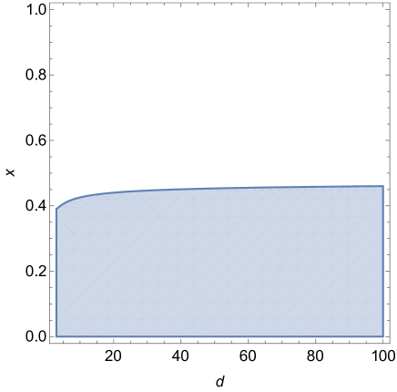
Figure 1: The shaded region shows the range of the parameter $x$ in which the channel $\Phi_{x}$ has a positive quantum capacity. Interestingly the cricial value is approximately equal to $0.4$ for all dimensions. Above this critical value, the coherent information is negative and it is not known if the channel $\Phi_{x>x_{0}}$ has a non-zero quantum capacity.

6.1 On the anti-degradability of the pure LS channel

An interesting open question is whether or not the pure so(d) is anti-degradable (as it was for the $d=3$ case). For the so(3) case, this was evident. In fact the relation from the form of the Kraus operators (7) and the relation $(R_{i})_{\alpha,j}=(A_{\alpha})_{ij}$, it turned out that the Kraus operators of the channel and its complement are equal, hence the two channels were identical, implying that the so(3) channel is both degradable and anti-degradable. For higher values of $d$, the channel has $\frac{d(d-1)}{2}$ Kraus operators, each of dimension $d$. Hence the two channels will not be identical. One can determine the closed form of the complement of the pure so(d) LS channel (without the noise term) along the same line that was outlined in section (5). We rewrite the channel $\Phi_{1}$ as

$$\Phi_{-}(\rho)=\frac{1}{2(d-1)}\sum_{m,n}J_{mn}\rho J_{mn}^{\dagger}$$ (81)

and hence

$$\Phi_{-}^{c}(\rho)=\sum_{i}R_{i}\rho R_{i}^{\dagger},\hskip 28.45274pt(R_{i})_{mn,j}=(A_{mn})_{ij}=\frac{1}{\sqrt{2(d-1)}}\langle i|J_{mn}|j\rangle=-i\frac{1}{\sqrt{2(d-1)}}(\delta_{im}\delta_{nj}-\delta_{ni}\delta_{mj}).$$ (82)

Inserting these in the expression of the channel and summing over all the dummy indices and simplifying, we find

$$\Phi_{-}^{c}(\rho)=\frac{1}{2(d-1)}\left[(I\otimes\rho+\rho\otimes I)(I-S)\right]$$ (83)

where $S$ is the swap operator. Note that we have used the anti-symmetry of the Kraus operators $A_{mn}$ to sum over all $m$ and $n$ and this has led to a $d^{2}$ matrix $\Phi^{c}_{1}(\rho)$. At first, one is tempted to guess that the channel $\Psi(\rho):=Tr_{2}(\rho)$ may connect this channel to $\phi_{-}$ hence prove its anti-degradability, however it turns out that

$$(\Psi\circ\Phi_{-}^{c})(\rho)=Tr_{2}(\Phi_{-}^{c}(\rho))=\frac{1}{2(d-1)}(\tr(\rho)I+(d-2)\rho)$$ (84)

which is different from $\Phi_{-}$. Therefore the question of (anti)-degradability of the so(d) channel remains to be investigated.

Note that the reason that in the so(3) case, the channel and its complement are the same [14] and hence the so(3) channel is both degradable and anti-degradable, is the identification of anti-symmetric tensors with vectors, which does not hold in higher dimensions.

7 $u(d)$ generalization of the Landau-Streater channel

In this section, we briefly mention how the LS channel can be generalized to the group $u(d)$. Let us replace the set $A_{-}$ with the following set of operators $A_{+}=\{K_{mn},1\leq m,n\leq d\}$ where

$$K_{mn}=|m\rangle\langle n|+|n\rangle\langle m|,\ \ \ m<n,\hskip 28.45274ptK_{mm}=2|m\rangle\langle m|.$$ (85)

The set $A_{+}$ of dimension $\frac{d(d+1)}{2}$ is not closed under the Lie-bracket and hence is not a Lie-algebra anymore. However the combined set $A=A_{-}\cup A_{+}$ forms the Lie-Algebra of the group $U(d)$ of $d$-dimensional unitary matrices. Note that dimension of $A$, i.e. is equal to $d^{2}$ which is equal to the dimension of the group $U(d)$. One can show by direct calculation that

$$\frac{1}{2}\sum_{m,n}K_{mn}^{\dagger}K_{mn}=(d+1)\ \mathcal{I}.$$ (86)

Therefore one can define another quantum channel as follows

$$\phi_{+}(\rho):=\frac{1}{2(d+1)}\sum_{m,n}K_{mn}\rho K_{mn}^{\dagger}=\frac{1}{d+1}\left[\tr\rho\ \mathcal{I}+\rho^{T})\right]$$ (87)

This is a new generalization of the Landau-Streater channel which is equivalent to the Werner-Holevo channel $\phi_{{}_{1,d}}$. Its complement is the same as in (83), except that $I-S$ is replaced with $I+S$. Note that the Kraus opeators $K_{mn}$ are not generators of a Lie algebra anymore. Despite this, the covariance under $U(d)$ holds for both channels, that is

$$\phi^{\pm}(U\rho U^{\dagger})=U^{*}\phi^{\pm}(\rho)U^{T}\hskip 28.45274ptU\in U(d)$$ (88)

where $U(d)$ is the group of unitary operators on $\mathcal{H}$. We can now make the following convex combination of these channels to arrive at a one-parameter family of channels:

$$\phi_{{\eta,d}}(\rho)=\frac{1-\eta}{2}\phi_{-}(\rho)+\frac{1+\eta}{2}\phi_{+}(\rho)$$ (89)

which turns out to be equal to the one-parameter family of Werner-Holevo channels in equation (4) [2]. The Kraus operators are now the set of generators of the Lie-Algebra $u(d)$, namely the set $\{J_{mn},\ K_{mn}\}$. Therefore we call this The u(d) Landau-Streater channel. One also modify this channel to represent a two-parameter family of noisy su(d) LS-channels by defining a convex combination of the identity channel, $\phi_{-}$ and $\phi_{+}$.

8 Discussion

We have generalized the Landau-Streater channel which is pertaining to the spin-j representation of the Lie-algebra $so(3)$ to the fundamental representation of the groups $so(d)$ and and have pointed out their equivalence to the Werner-Holevo channels. We have studied several properties of the resulting one-parameter family of quantum channels, including their spectrum, their region of infinitesimal divisibility, their complement channels and finally their one-shot classical capacity and their entanglement-assisted classical capacity. It would be an interesting problem if one can define and study the Landau-Streater channel in a most general setting, namely any representation of any Lie-algebra [34]. Certainly these kinds of channels may not find concrete applications in quantum information processing, but they are definitely of great interest in the structural theory of quantum channels and completely positive maps. Even for the so(d) groups and the representation we have used, our study can lead to many extensions, the immediate one will be to study their approximate degradability along the lines of the recent work [15].

9 Acknowledgements

I would like to thank members of the QIS group in Sharif, especially Shayan Roofeh for their valuable comments.

References

• [1] L.ย J. Landau and R.ย F. Streater. On birkhoffโ€™s theorem for doubly stochastic completely positive maps of matrix algebras. Linear Algebra and its Applications, 193:107, 1993.
• [2] R.ย F. Werner and A.ย S. Holevo. Counterexample to an additivity conjecture for output purity of quantum channels. Journal of Mathematical Physics, 43:4353, 2002.
• [3] Koenraad Mย R Audenaert and Stefan Scheel. On random unitary channels. New Journal of Physics, 10(2):023011, February 2008.
• [4] Sergeyย N. Filippov and Kseniaย V. Kuzhamuratova. Quantum informational properties of the Landauโ€“Streater channel. Journal of Mathematical Physics, 60(4):042202, April 2019.
• [5] A.ย I. Pakhomchik, I.ย Feshchenko, A.ย Glatz, V.ย M. Vinokur, A.ย V. Lebedev, S.ย N. Filippov, and G.ย B. Lesovik. Realization of the Wernerโ€“Holevo and Landauโ€“Streater Quantum Channels for Qutrits on Quantum Computers. Journal of Russian Laser Research, 41(1):40โ€“53, January 2020.
• [6] Mark Girard, Debbie Leung, Jeremy Levick, Chi-Kwong Li, Vern Paulsen, Yiuย Tung Poon, and John Watrous. On the mixed-unitary rank of quantum channels. Communications in Mathematical Physics, 394(2):919โ€“951, June 2022.
• [7] Nilanjana Datta, Alexanderย S. Holevo, and Yuri Suhov. Additivity for transpose depolarizing channels, 2004.
• [8] Thomas P.ย W. Cope and Stefano Pirandola. Adaptive estimation and discrimination of holevo-werner channels. Quantum Measurements and Quantum Metrology, 4(1), December 2017.
• [9] Thomas Pย W Cope, Kenneth Goodenough, and Stefano Pirandola. Converse bounds for quantum and private communication over holevoโ€“werner channels. Journal of Physics A: Mathematical and Theoretical, 51(49):494001, November 2018.
• [10] Eric Chitambar, Ian George, Brian Doolittle, and Marius Junge. The communication value of a quantum channel. IEEE Transactions on Information Theory, 69(3):1660โ€“1679, March 2023.
• [11] Mย M Wolf and Jย Eisert. Classical information capacity of a class of quantum channels. New Journal of Physics, 7:93โ€“93, April 2005.
• [12] KMR Audenaert and Sย Scheel. On random unitary channels. New Journal of Physics, 10(2):023011, 2008.
• [13] Michael Horodecki, Peterย W. Shor, and Maryย Beth Ruskai. Entanglement breaking channels. Reviews in Mathematical Physics, 15(06):629โ€“641, August 2003.
• [14] Shayan Roofeh and Vahid Karimipour. The noisy werner-holevo channel and its properties, 2023.
• [15] Yun-Feng Lo, Yen-Chi Lee, and Min-Hsiu Hsieh. Degradability of modified landau-streater type low-noise quantum channels in high dimensions, 2024.
• [16] David Sutter, Volkherย B. Scholz, Andreas Winter, and Renato Renner. Approximate degradable quantum channels. IEEE Transactions on Information Theory, 63(12):7832โ€“7844, December 2017.
• [17] I.ย Devetak and P.ย W. Shor. The Capacity of a Quantum Channel for Simultaneous Transmission of Classical and Quantum Information. Communications in Mathematical Physics, 256(2):287โ€“303, June 2005.
• [18] Tobyย S. Cubitt, Maryย Beth Ruskai, and Graeme Smith. The structure of degradable quantum channels. Journal of Mathematical Physics, 49(10):102104, October 2008.
• [19] Michaelย M. Wolf and J.ย Ignacio Cirac. Dividing Quantum Channels. Communications in Mathematical Physics, 279(1):147โ€“168, April 2008.
• [20] A.ย S. Holevo. Remarks on the classical capacity of quantum channel, December 2002. arXiv:quant-ph/0212025.
• [21] In Markย M. Wilde, editor, Quantum Information Theory, pages xiโ€“xii. Cambridge University Press, Cambridge, 2 edition, 2017.
• [22] Charlesย H. Bennett, Peterย W. Shor, Johnย A. Smolin, and Ashishย V. Thapliyal. Entanglement-Assisted Classical Capacity of Noisy Quantum Channels. Physical Review Letters, 83(15):3081โ€“3084, October 1999.
• [23] C.H. Bennett, P.W. Shor, J.A. Smolin, and A.V. Thapliyal. Entanglement-assisted capacity of a quantum channel and the reverse Shannon theorem. IEEE Transactions on Information Theory, 48(10):2637โ€“2655, October 2002.
• [24] Howard Barnum, M.ย A. Nielsen, and Benjamin Schumacher. Information transmission through a noisy quantum channel. Physical Review A, 57(6):4153โ€“4175, June 1998.
• [25] A.ย S. Holevo. Complementary Channels and the Additivity Problem. Theory of Probability & Its Applications, 51(1):92โ€“100, January 2007.
• [26] A.ย S. Holevo. Quantum systems, channels, information: a mathematical introduction. Numberย 16 in De Gruyter studies in mathematical physics. De Gruyter, Berlin, 2012.
• [27] W.ย Forrest Stinespring. Positive Functions on C * -Algebras. Proceedings of the American Mathematical Society, 6(2):211, April 1955.
• [28] N.ย Datta, M.ย Fukuda, and A.ย S. Holevo. Complementarity and Additivity for Covariant Channels. Quantum Information Processing, 5(3):179โ€“207, June 2006.
• [29] Marek Smaczyล„ski, Wojciech Roga, and Karol ลปyczkowski. Selfcomplementary Quantum Channels. Open Systems & Information Dynamics, 23(03):1650014, September 2016.
• [30] Howard Barnum, M.ย A. Nielsen, and Benjamin Schumacher. Information transmission through a noisy quantum channel. Physical Review A, 57(6):4153โ€“4175, June 1998.
• [31] Seth Lloyd. Capacity of the noisy quantum channel. Physical Review A, 55(3):1613โ€“1622, March 1997.
• [32] Peter Shor. Quantum error correction, 2002.
• [33] I.ย Devetak. The private classical capacity and quantum capacity of a quantum channel. IEEE Transactions on Information Theory, 51(1):44โ€“55, January 2005.
• [34] Williamย Gordon Ritter. Quantum channels and representation theory. Journal of Mathematical Physics, 46(8), August 2005.