Optimal consumption and investment under relative performance criteria with Epstein-Zin utility

Abstract.

We consider the strategic interaction of traders in a continuous-time financial market with Epstein-Zin-type recursive intertemporal preferences and performance concerns. We derive explicitly an equilibrium for the finite player and the mean-field version of the game, based on a study of geometric backward stochastic differential equations of Bernoulli type that describe the best replies of traders. Our results show that Epstein-Zin preferences can lead to substantially different equilibrium behavior.

Keywords: Mean field games, portfolio choice, recursive utility, stochastic differential utility, BSDEs

AMS subject classification: 93E20, 91A15, 91A30, 60H10, 60H30.

JEL classification: C02, C61, C61, C73, G11.

1. Introduction

Casual observations as well as empirical evidence suggest that relative performance concerns play a significant role in the decision-making of traders. Many fund managers are evaluated based on their performance relative to a benchmark index or their peers, creating pressure to match or exceed the performance of others in the industry.

In this paper, we consider the strategic interaction of such traders with performance concerns when intertemporal preferences are recursive, of the Epstein-Zin type ([10], [11]), thus extending the previous work of [12], [20] and [19] to this important class of intertemporal preferences. The time-additive discounted utility model is restrictive in many senses. In particular, it does not allow to disentangle the conceptually and empirically different concepts of risk aversion and intertemporal elasticity of substitution. Epstein-Zin preferences are among the few tractable versions of stochastic differential utility that allow to make this distinction.

This game’s Nash equilibrium can be derived in closed-form despite the intricate interplay between recursive preferences, continuous-time financial markets, and relative performance concerns (see Theorem 2.2). We are also able to consider the mean-field version of the game involving potentially a continuum of players (see Theorem 2.6). Our study is the first example of a mean-field game involving stochastic differential utility functions.

Allowing for recursive preferences has important consequences for equilibrium behavior. We show that assuming time-additive utilities might lead to quite misleading conclusions (see Section 2.3). For example, assuming a usual parameter of relative risk aversion above $1$, one implicitly assumes a rate of intertemporal elasticity of substitution smaller than 1, while empirically one frequently observes a rate of intertemporal elasticity of substitution above 1, see the discussion in [14, p. 574] and [2]. We show that the intertemporal consumption pattern can be completely reversed when one allows for this distinction.

We also show that the parameter of risk aversion alone determines portfolio choice. The rate of intertemporal elasticity of substitution plays a more significant role in determining consumption patterns, in line with the literature on Epstein-Zin preferences for single agents (e.g., see [18]).

Our problem embeds into stochastic differential games, that are popular models describing competition in a random environment, with countless applications in finance and economics. [13, 21] introduced the mean-field game as the limit model when the number of players goes to infinity, thus providing tools to construct approximate Nash equilibria in games involving a large number of players. Several approaches exist to solve such games, including systems of partial differential equations and of forward-backward stochastic differential equations, see the textbooks [4, 5] for a detailed description.

Despite the extensive literature and the general abstract existence and characterization results, many approaches encounter computational challenges due to the high dimensionality of the involved equations. Consequently, numerical analysis of equilibria remains highly problematic, even for scenarios with a limited number of players. This underscores the significance of the few explicitly solvable models in the literature and highlights the importance of discovering new ones.

From the methodological point of view, our approach is based on the analysis of systems of backward stochastic differential equations with Bernoulli driver, that we call Bernoulli BSDEs, see Section 3. Best replies in our game can be expressed in terms of the solutions to such Bernoulli BSDEs and we are thus able to derive a Nash equilibrium for the finite player and mean-field game that are unique in the class of simple (deterministic) strategies. Indeed, optimization problems with Epstein-Zin recursive utility are known to be related to Bernoulli ordinary differential equations or to partial differential equations with some terms of Bernoulli type as in [18].

In the game context, the optimization problem of the one player is parameterized by the actions of its opponents, and the resulting optimization problem is expressed in terms of a Bernoulli BSDE which does not reduce to an ODE. Despite Bernoulli BSDEs having no Lipschitz driver, our explicit analysis allows us to show that these equations can successfully be used to demonstrate the existence of the equilibria as well as to recover the usual convergence and approximation results relating Nash equilibria and mean field game equilibria, thus justifying the mean-field game as the limit of the finite player game.

We finally underline the nature of our mean-field game equilibrium. When the noises affecting players’ decisions are correlated, a common noise appears in the limiting mean-field game and technical challenges arise. Indeed, the equilibrium actions become (in general) only conditionally independent of the future realization of the common noise (see [6]), and only few cases are known in which these are actually adapted to the common source of randomness (see e.g. [1, 6, 9, 19] among others). Our explicit analysis allows to find an equilibrium of the latter type.

Related literature

We consider the dynamic problem of consumption and portfolio choice formalized and studied in the landmark papers of Merton [23, 24]. Other papers such as [8] that incorporated multiple agents into the Merton model, did so in a general equilibrium context; in contrast, in our work agents are price-takers in our model, and we do not attempt to incorporate price equilibrium. Interaction between agents in our model comes from a mean field interaction through both the states and controls (see [5, Vol. I, Chapter 4.6]). This approach has been developed by a recent literature that considered the case of standard utility [19, 20] (see also [22] for the case of habit formation without common noise). Our novelty relies on building on the literature on dynamic portfolio choice problems with stochastic differential utility started by [10] (see [25, 18, 3, 17] for more recent papers in the literature we build on).

As fas ar the more mathematical literature is concerned, our study belongs to the class of stochastic differential and mean-field games ([13, 21], [4, 5]). Solvable games of major relevance are essentially of two types. In linear-quadratic games, the equilibria correspond to solutions of systems of Riccati equations. While an extensive literature addresses these games (see [4] and the references therein), recent applications in finance involved the systemic risk analysis of banking networks (see [7]). The other class (which is more similar to our model) is the case in which dynamics are geometric and utility functions exhibit constant relative risk aversion type. These models were studied in continuous time frameworks in the quite recent papers [19, 20], for both finite player games and mean field games, in order to address portfolio optimization problems for competitive agents. Within this framework, our work shows that the relevant case of games with geometric dynamics and Epstein-Zin utility is still explicitly solvable. Whether the same could be true for linear-quadratic models combined with suitable types of recursive utility remains an open problem that we address with future research. More generally, our work suggests that it is possible to develop a mean field theory for stochastic differential games with recursive utility.

Structure

The next section describes the model and presents the main results on the finite player and mean-field games, including a discussion of the economic relevance of our results. Section 3 contains the independent results on geometric Bernoulli Backward Stochastic Differential Equations. Section 4 is devoted to the proofs of the main results. Section 5 provides concluding remarks.

2. Main Results

To start with, we introduce the aggregator and the bequest function that will characterize the intertemporal preferences of our agents. For a discount rate $\eta>0$, relative risk aversion $\gamma>0$, elasticity of intertemporal substitution $\delta>0$, and a weight of bequest utility $\epsilon>0$ we assume throughout

(1) $$\gamma,\delta\not=1,\quad\text{and either $\gamma\delta,\,\delta\geq 1$ or $\gamma\delta,\,\delta\leq 1$.}$$

We also define $\lambda:=\frac{1-\gamma}{1-\frac{1}{\delta}}$ and $q:=1-\frac{1}{\lambda}$.

The Epstein-Zin aggregator $f$ and the bequest utility function $g$ are given by

(2) $$f(C,v;\delta,\gamma,\eta):=\eta\lambda v\left(\left(\frac{C}{((1-\gamma)v)^{\frac{1}{1-\gamma}}}\right)^{1-\frac{1}{\delta}}-1\right)g(C;\gamma,\epsilon,\eta)=\frac{(\eta\epsilon)^{\lambda}}{1-\gamma}C^{1-\gamma},$$

on the domain $C>0$ and $(1-\gamma)v>0$.

2.1. N-player Games with Epstein-Zin Preferences

We next describe the game that $N\in\mathbb{N}$ investors with relative performance concerns and recursive utility play. Investors’ preferences are characterized by the Epstein-Zin aggregators

$$f_{i}(C,v):=f(C,v;\delta_{i},\gamma_{i},\eta_{i})$$

and bequest utility functions

$$g_{i}(C,v):=g(C,v;\gamma_{i},\epsilon_{i},\eta_{i}),$$

for $f$ and $g$ defined in (2) with our standing assumption (1) on the parameters $\gamma_{i},\delta_{i}$.

The investors have access to financial markets as in [19]. Take independent Brownian motions $B,W^{1},...,W^{N}$ on a given complete probability space $(\Omega,\mathcal{F},\mathbb{P})$ and denote by $\mathbb{F}^{N}:=(\mathcal{F}^{N}_{t})_{t\in[0,T]}$ the right-continuous extension of the filtration generated by $B,W^{1},...,W^{N}$, augmented by the $\mathbb{P}$-null sets. A (consumption–portfolio) strategy (or policy) $\alpha=(c,\pi)$ is a couple of $(0,\infty)\times\mathbb{R}$-valued $\mathbb{F}^{N}$-progressively measurable processes such that the boundedness conditions

(3) $$0<\operatorname*{ess\,inf}c\leq\operatorname*{ess\,sup}c<\infty\operatorname*{ess\,sup}|\pi|<\infty,$$

are satisfied. We denote by $\mathcal{A}_{N}$ the set of consumption-portfolio strategies. Policies will be denoted either by $\alpha_{i}=(c_{i}(t),\pi_{i}(t))_{t\in[0,T]}$ or by $\alpha=(c_{t},\pi_{t})_{t\in[0,T]}$, depending on whether we want to refer to the specific investor $i$ or not. A strategy $\alpha=(c,\pi)$ is simple if

(4) $$c \pi\in\mathbb{R}$$ is a deterministic function and is a constant.

A strategy profile $\bm{\alpha}=(\alpha_{1},...,\alpha_{N})$ is said to be simple if $\alpha_{i}$ is a simple strategy for any $i=1,...,N$.

For a policy $\alpha_{i}$, the wealth process of investor $i$ is given by

(5) $$dX^{i}_{t}=\pi_{i}(t)X_{t}^{i}(\mu_{i}dt+\nu_{i}dW^{i}_{t}+\sigma_{i}dB_{t})-c_{i}(t)X^{i}_{t}dt,\quad X^{i}_{0}=x^{i}_{0}$$

for initial wealth $x^{i}_{0}>0$, idiosyncratic volatility $\nu_{i}\geq 0$, common volatility $\sigma_{i}\geq 0$ with $\nu_{i}+\sigma_{i}>0$ and drift $\mu_{i}\in\mathbb{R}$.

The utility process $(V_{t}^{i}{(\bm{\alpha})})_{t\in[0,T]}$ of investor $i$ is given by the solution to the backward stochastic differential equation (BSDE, in short)

(6) $$V_{t}^{i}{(\bm{\alpha})}=\mathbb{E}\left[\left.\int_{t}^{T}f_{i}\left(c_{i}(s)X_{s}^{i}(\overline{c}_{s}\overline{X}_{s})^{-\theta_{i}},V_{s}^{i}{(\bm{\alpha})}\right)ds+g_{i}\left(X_{T}^{i}\overline{X}_{T}^{-\theta_{i}}\right)\right|\mathcal{F}_{t}\right].$$

The strategic interaction among players derives from the relative performance concerns modeled through the geometric averages of consumption and wealth

$$\overline{X}_{t}:=\Big{(}\prod_{j=1}^{N}X_{t}^{j}\Big{)}^{1/N}\quad\text{and}\quad\overline{c}_{t}:=\Big{(}\prod_{j=i}^{N}c_{j}(t)\Big{)}^{1/N}.$$

Remark 2.1.

1. For any strategy profile $\bm{\alpha}$, the utility process defined by the BSDE (6) is well-defined by Theorem 3.1 in [25] (see also [18] for stochastic differential utilities in a context similar to ours in which $c$ is not necessarily continuous). Indeed, Theorem 3.1 in [25] yields existence and uniqueness of $V^{i}(\bm{\alpha})$ provided that the process $P_{t}^{\bm{\alpha}}:=c_{i}(t)X_{t}^{i}(\overline{c}_{t}\overline{X}_{t})^{-\theta}$ is positive and satisfies

   $$\mathbb{E}\Big{[}\int_{0}^{T}|P_{t}^{\bm{\alpha}}|^{k}dt+|P_{T}^{\bm{\alpha}}|^{k}\Big{]}<\infty,\quad\text{for any $k\in\mathbb{R}$.}$$

   The latter integrability easily follows from the condition (3) in the definition of strategies $\alpha_{i}$.

2. In the case of $\gamma_{i}=\frac{1}{\delta_{i}}$, we recover the case of time–additive intertemporal preferences. Indeed, using Itô’s lemma, one can show that the ordinally equivalent utility process

   $$U^{i}_{t}:=\frac{1}{\eta_{i}}\left(V_{t}^{i}{(\bm{\alpha})}\right)^{\frac{1}{\lambda}}$$

   satisfies the equation

   $$U^{i}_{t}=\mathbb{E}\left[\int_{t}^{T}e^{-\eta_{i}(s-t)}\frac{(c_{i}(s)X_{s}^{i}(\overline{c}_{s}\overline{X}_{s})^{-\theta_{i}})^{1-\gamma_{i}}}{1-\gamma_{i}}ds+\epsilon_{i}\frac{(X_{T}^{i}\overline{X}_{T}^{-\theta_{i}})^{1-\gamma_{i}}}{1-\gamma_{i}}\right].$$

   This parametrization of investor i’s preferences shows that $\epsilon_{i}$ is indeed to be interpreted as the weight of the bequest utility, justifying our choice of the factor $(\eta\epsilon)^{\lambda}$ in Equation (2).

   In particular, we cover the time-additive case for non-zero discount rates that was not solved for in [19], where both the safe interest rate and the discount rate are zero. Such an assumption does not come without loss of generality. Thus, it is economically important to study the case of distinct interest and discount rate.

Given a strategy profile $\bm{\alpha}=(\alpha_{i})_{i=1,\ldots,N}\in\mathcal{A}_{N}^{N}$, denote by $\bm{\alpha}_{-i}:=(\alpha_{j})_{j\neq i}$ the vector of strategies chosen by investors $j\neq i$ and write, as usual in game theory, $\bm{\alpha}=(\alpha_{i},\bm{\alpha}_{-i}):=(\alpha_{1},...,\alpha_{N})\in\mathcal{A}_{N}^{N}$. A strategy profile $\hat{\bm{\alpha}}$ is a Nash equilibrium (NE, in short) if

(7) $$V_{0}^{i}(\hat{\bm{\alpha}})\geq V_{0}^{i}(\alpha_{i},\hat{\bm{\alpha}}_{-i}), \alpha_{i}\in\mathcal{A}_{N} i=1,...,N$$ for any and .

Theorem 2.2.

There exists a unique Nash equilibrium in simple strategies $\hat{\bm{\alpha}}_{N}=(\hat{\alpha}_{1,N},...,\hat{\alpha}_{N,N})$ given by

(8) $$\hat{\pi}_{i,N} ={\frac{1}{\gamma_{i}}}\frac{\mu_{i}}{(1+\frac{\theta_{i}}{N}(\frac{1}{\gamma_{i}}-1))\nu_{i}^{2}+\sigma_{i}^{2}}-{\sigma_{i}}\theta_{i}\big{(}\frac{1}{\gamma_{i}}-1\big{)}\frac{\Pi_{N}}{(1+\frac{\theta_{i}}{N}(\frac{1}{\gamma_{i}}-1))\nu_{i}^{2}+\sigma_{i}^{2}},$$

(9) $$\hat{c}_{i,N}(t) =\begin{cases}\Big{(}\frac{1}{{\chi_{2}^{i,N}}}+\big{(}\frac{1}{\chi_{1}^{i,N}}-\frac{1}{\chi_{2}^{i,N}}\big{)}e^{-\chi_{2}^{i,N}(T-t)}\Big{)}^{-1}&\text{ if }\chi_{2}^{i,N}\neq 0,\\ \big{(}T-t+\frac{1}{\chi_{1}^{i,N}}\big{)}^{-1}&\text{ if }\chi_{2}^{i,N}=0,\end{cases}$$

where

$$\Pi_{N} =\frac{E_{N}}{1+F_{N}},$$

$$E_{N} =\frac{1}{N}{\sum_{j=1}^{N}\frac{\sigma_{j}\mu_{j}}{{\gamma_{j}}{(1+\frac{\theta_{j}}{N}(\frac{1}{\gamma_{j}}-1))\nu_{j}^{2}+\gamma_{j}\sigma_{j}^{2}}}},$$

$$F_{N} ={\frac{1}{N}\sum_{j=1}^{N}\frac{{\sigma_{j}^{2}}\theta_{j}(1-\gamma_{j})}{{\gamma_{j}}{(1+\frac{\theta_{j}}{N}(\frac{1}{\gamma_{j}}-1))\nu_{j}^{2}+\gamma_{j}\sigma_{j}^{2}}}},$$

$$\chi_{1}^{i,N} =\epsilon_{i}^{-\delta_{i}}\Big{(}\prod_{j=1}^{N}\epsilon_{j}^{-\delta_{j}}\Big{)}^{\frac{\theta_{i}(1-\delta_{i})}{N-\sum_{j=1}^{N}\theta_{j}(1-\delta_{j})}},$$

$$\chi_{2}^{i,N} =-\frac{\delta_{i}}{\lambda_{i}}\rho_{i,N}-\theta_{i}(1-\delta_{i})\frac{\sum_{j=1}^{N}\frac{\delta_{j}}{\lambda_{j}}\rho_{j,N}}{N-\sum_{j=1}^{N}\theta_{j}(1-\delta_{j})},$$

$$\rho_{i,N} =-\eta_{i}\lambda_{i}+(1-\gamma_{i})\Big{[}-\theta_{i}\hat{\mu}_{i}+\frac{1}{2}\theta_{i}(1+\theta_{i}(1-\gamma_{i}))(\hat{\nu}_{i}^{2}+\hat{\sigma}_{i}^{2})$$

$$\quad\quad\quad\quad\quad\quad\quad\quad\quad-\frac{1}{2}(1-\frac{\theta_{i}}{N})\frac{(\sigma_{i}\hat{\sigma}_{i}\theta_{i}(1-\gamma_{i})-\mu_{i})^{2}}{((1-\frac{\theta_{i}}{N})(1-\gamma_{i})-1)(\nu_{i}^{2}+\sigma_{i}^{2})}\Big{]},$$

$$\hat{\nu}_{i} =\frac{1}{N}\sqrt{\sum_{j\neq i}(\nu_{j}\hat{\pi}_{j,N})^{2}},\quad\hat{\sigma}_{i}=\frac{1}{N}\sum_{j\neq i}\sigma_{j}\hat{\pi}_{j,N},$$

$$\hat{\mu}_{i} =\frac{1}{N}\sum_{j\neq i}\big{(}\mu_{j}\hat{\pi}_{j,N}-\frac{1}{2}\hat{\pi}_{j,N}^{2}(\nu_{j}^{2}+\sigma_{j}^{2})\big{)}+\frac{1}{2}(\hat{\nu}_{i}^{2}+\hat{\sigma}_{i}^{2}).$$

Corollary 2.3.

In the case of a single common stock, i.e. $\nu_{i}=0$ for all $i$, a common drift $\mu_{i}=\mu$ and common volatility $\sigma_{i}=\sigma$, the Nash equilibrium strategies simplify to

$$\hat{\pi}_{i,N} =\frac{1}{\gamma_{i}}\frac{\mu}{\sigma^{2}}-\theta_{i}\left(\frac{1}{\gamma_{i}}-1\right)\frac{\mu}{\sigma^{2}}\frac{\frac{1}{N}\sum_{j=1}^{N}\frac{1}{\gamma_{j}}}{1+\frac{1}{N}\sum_{j=1}^{N}\theta_{j}\left(\frac{1}{\gamma_{j}}-1\right)},$$

$$\hat{c}_{i,N}(t) =\begin{cases}\left(\frac{1}{{\chi_{2}^{i,N}}}+\big{(}\frac{1}{\chi_{1}^{i,N}}-\frac{1}{\chi_{2}^{i,N}}\big{)}e^{-\chi_{2}^{i,N}(T-t)}\right)^{-1}&\text{ if }\chi_{2}^{i,N}\neq 0,\\ \left(T-t+\frac{1}{\chi_{1}^{i,N}}\right)^{-1}&\text{ if }\chi_{2}^{i,N}=0,\end{cases}$$

2.2. Mean-Field Games with Epstein-Zin Preferences

We now introduce the mean-field game following the notation of [19, 20]. Let the probability space $(\Omega,\mathcal{F},P)$ be endowed with a filtration $\mathbb{F}=(\mathcal{F}_{t})_{t\in[0,T]}$ satisfying the usual conditions. Let $B$ and $W$ be independent $\mathbb{F}$-Brownian motions, modeling common and idiosyncratic noise, resp. We underline that the $\sigma$-algebra $\mathcal{F}_{0}$ is independent from $B$ and $W$, but it is not necessarily trivial.

The representative investor is characterized by the initial wealth $x_{0}$, the drift and volatility parameters of her stock $\mu,\nu,\sigma$, and the preference parameters $\gamma,\delta,\epsilon,\eta,\theta$. We call

$$\mathcal{I}:=(0,\infty)\times\mathbb{R}\times[0,\infty)\times[0,\infty)\times(0,\infty)\times(0,\infty)\times(0,\infty)\times[0,1]$$

the corresponding type space of our game with typical element $(x_{0},\mu,\nu,\sigma,\eta,\gamma,\delta,\epsilon,\theta)$. The type of representative investor is described by a $\mathcal{F}_{0}$-measurable random variable $\mathcal{T}:\Omega\rightarrow\mathcal{I}$, and we assume

(10) $$\sigma+\nu>0,\quad\gamma,\delta\not=1,\quad\text{and either $\gamma\delta,\,\delta\geq 1$ or $\gamma\delta,\,\delta\leq 1$, \quad$\mathbb{P}$-a.s.}$$

The Epstein-Zin aggregator $f$ and terminal cost $g$ of the representative investor are respectively given by the (random) functions

$$f:=f(\cdot;\delta,\gamma,\eta)\quad\text{and}\quad g:=g(\cdot;\gamma,\epsilon,\eta),$$

for $f$ and $g$ defined in (2).

A (consumption-investment) policy $\alpha=(c,\pi)$ is a couple of $(0,\infty)\times\mathbb{R}$-valued $\mathbb{F}$-progressively measurable processes such that the boundedness conditions (3) are satisfied. We denote by $\mathcal{A}$ the set of policies. A strategy $\alpha=(c,\pi)$ is said to be simple if

(11) $$c \mathcal{F}_{0} \pi \mathcal{F}_{0}$$ is -measurable and is -measurable constant in time.

For a policy $\alpha$, the wealth process of the representative investor is given by

(12) $$dX_{t}=\pi_{t}X_{t}(\mu dt+\nu dW_{t}+\sigma dB_{t})-c_{t}X_{t}dt,\quad X_{0}=x_{0}.$$

Let $\mathbb{F}^{B}=(\mathcal{F}^{B}_{t})_{t\in[0,T]}$ denote the natural filtration of the Brownian motion $B$. We denote by $Y$ and $m$ the generic geometric mean wealth and geometric mean consumption rate of the population of investors, respectively. The processes $Y$ and $m$ are assumed to be $\mathbb{F}^{B}$-progressively measurable. The representative investor takes $Y$ and $m$ as given, and aims at maximizing, over the policy $\alpha$, her utility $V=V(\alpha;m,Y)$ which is given by the solution to the BSDE

(13) $$V_{t}=\mathbb{E}\left[\left.\int_{t}^{T}f\left(c_{s}X_{s}\left(m_{s}Y_{s}\right)^{-\theta},V_{s}\right)ds+g\left(X_{T}Y_{T}^{-\theta}\right)\right|\mathcal{F}_{t}\right].$$

Remark 2.4.

The existence of stochastic differential utility $V$ solving (13) with random initial parameters can be shown along the lines of [25] (see also Remark 2.1). In fact, existence of SDU when initial wealth $x_{0}$, drift $\mu$ and $\nu$ and volatility $\sigma$ are random $\mathcal{F}_{0}$-measurable variables is already covered by Theorem 3.1 in [25]. The authors do not discuss the case of random initial preference parameters $(\delta,\gamma,\epsilon,\theta,\eta)$, though, yet an inspection of the proofs shows that the arguments go through.

Using a martingale representation argument, one can show that the process $V$ solving (13) satisfies the backward stochastic differential equation

$$dV_{t}=-f(c_{t}X_{t}(m_{t}Y_{t})^{-\theta},V_{t})dt+Z^{1}_{t}dW_{t}+Z^{2}_{t}dB_{t},\quad V_{T}=g(X_{T}Y_{T}^{-\theta}),$$

for some square-integrable progressively measurable processes $Z^{i},i=1,2$.

In equilibrium, the assumed geometric mean consumption rate $m$ has to be equal to the geometric mean consumption rate of the population that is given by

$$\exp(\mathbb{E}[\log c_{t}|\mathcal{F}^{B}_{t}])$$

and the assumed geometric mean wealth has to equal the population geometric mean wealth

$$\exp(\mathbb{E}[\log Y_{t}|\mathcal{F}^{B}_{t}]).$$

We refer to [19, 20] for more details.

Definition 2.5.

Let $\hat{\alpha}=(\hat{c},\hat{\pi})$ be a policy with corresponding wealth process $\hat{X}$. Let

$$\hat{Y}_{t}=\exp(\mathbb{E}[\log\hat{X}_{t}|\mathcal{F}^{B}_{t}])\hat{m}_{t}=\exp(\mathbb{E}[\log\hat{c}_{t}|\mathcal{F}^{B}_{t}]).$$

$\hat{\alpha}$ is a mean-field game equilibrium (MFGE) if $\hat{\alpha}$ maximizes the recursive utility $V(\cdot;\hat{m},\hat{Y})$.

Theorem 2.6.

There is a unique MFGE in simple strategies $\hat{\alpha}=(\hat{c},\hat{\pi})$ given by

$$\hat{\pi} =\frac{\mu}{\gamma(\sigma^{2}+\nu^{2})}-\theta\left(\frac{1}{\gamma}-1\right)\frac{\sigma}{(\sigma^{2}+\nu^{2})}\frac{E}{1+F},$$

$$\hat{c}_{t} =\begin{cases}\Big{(}\frac{1}{{\chi_{2}}}+\big{(}\frac{1}{\chi_{1}}-\frac{1}{\chi_{2}}\big{)}e^{-\chi_{2}(T-t)}\Big{)}^{-1}&\text{ if }\chi_{2}\neq 0,\\ \big{(}T-t+\frac{1}{\chi_{1}}\big{)}^{-1}&\text{ if }\chi_{2}=0,\end{cases}$$

where

$$E =\begin{matrix}{\mathbb{E}\left[\frac{\mu\sigma}{\gamma(\sigma^{2}+\nu^{2})}\right]}\end{matrix},$$

$$F =\begin{matrix}\mathbb{E}\left[\theta\left(\frac{1}{\gamma}-1\right)\frac{\sigma^{2}}{\sigma^{2}+\nu^{2}}\right]\end{matrix},$$

$$\chi_{1} =\epsilon^{-\delta}\exp\Big{(}\frac{\theta(1-\delta)}{1+\mathbb{E}[\theta(\delta-1)]}\mathbb{E}[-\delta\log\epsilon]\Big{)},$$

$$\chi_{2} =\theta(\delta-1)\frac{\mathbb{E}\left[\frac{\delta}{\lambda}\rho\right]}{1+\mathbb{E}\left[\theta(\delta-1)\right]}-\frac{\delta}{\lambda}\rho,$$

$$\rho :=-\eta\lambda+(1-\gamma)\Big{[}-\theta\hat{\mu}+\frac{1}{2}\theta(1+\theta(1-\gamma))\hat{\sigma}^{2}+\frac{1}{2}\frac{(\sigma\hat{\sigma}\theta(1-\gamma)-\mu)^{2}}{\gamma(\nu^{2}+\sigma^{2})}\Big{]},$$

$$\hat{\sigma} :=\mathbb{E}[\hat{\pi}\sigma],\quad\hat{\mu}:=\mathbb{E}[\hat{\pi}\mu]-\frac{1}{2}\big{(}\mathbb{E}[\hat{\pi}^{2}(\nu^{2}+\sigma^{2})]-(\mathbb{E}[\hat{\pi}\sigma])^{2}\big{)}.$$

2.3. The Economics of Relative Performance Concerns with Recursive Preferences

In the following, we discuss the new economic features of strategic behavior in equilibrium when relative performance concerns and recursive preferences matter. We focus mainly on the mean-field game, but emphasize the differences to finite player games in passing.

Let us start with the optimal portfolio choice. The optimal investment rule consists of the usual Samuelson-Merton term $\frac{\mu}{\gamma(\sigma^{2}+v^{2})}$ and a correction term for the relative performance concerns. Recursive utility allows to disentangle risk aversion $\gamma$ and elasticity of intertemporal substitution $\delta$. Note that the investment decision is affected by risk aversion, not by the elasticity of intertemporal substitution, a finding that reemphasizes the previous results in the literature on recursive preferences. Otherwise, the investment policy coincides with the investment policy of a time-additive investor with performance concerns in [19].

It is noteworthy to observe the scenarios in which the pure Merton portfolio emerges. This occurs when the investor disregards competitors, i.e. $\theta=0$. The Merton portfolio is also obtained in the case where $\gamma=1$, indicating an investor with unit relative risk aversion. Moreover, competition’s impact on investment diminishes when markets are entirely separate and independent ($\sigma=0$). This latter phenomenon is a mean-field effect. For finite $N$, competition influences portfolio selection, albeit diminishing with increasing $N$, as demonstrated in Equation (8).

In order to discuss the comparative statics of portfolio choice, we now consider the case of a common market without idiosyncratic noise.

Corollary 2.7.

Assume that $(\mu,\nu,\sigma)$ is deterministic with $\nu=0$ and $\mu,\sigma>0$. Then the optimal investment simplifies to

$$\pi_{\gamma}=\frac{\mu}{\sigma^{2}}\left(\frac{1}{\gamma}+\frac{\mathbb{E}[\frac{1}{\gamma}]\theta(1-\frac{1}{\gamma})}{(1+\mathbb{E}(\theta(\frac{1}{\gamma}-1)))}\right)$$

We have that

$$\diffp{\pi_{\gamma}}{\gamma}=\frac{\mu}{\sigma^{2}}\left(\frac{\theta\frac{\mathbb{E}[\frac{1}{\gamma}]}{1+\mathbb{E}(\theta(\frac{1}{\gamma}-1))}-1}{\gamma^{2}}\right),$$

so that if we set

$$\theta^{*}:=\frac{1+\mathbb{E}(\theta(\frac{1}{\gamma}-1))}{\mathbb{E}\left[\frac{1}{\gamma}\right]},$$

then whenever

$$\frac{\theta}{\theta^{*}}>1,$$

more risk aversion increases the level of investment in the portfolio, i.e. $\diffp{\pi_{\gamma}}{\gamma}>0$, while if

$$\frac{\theta}{\theta^{*}}<1,$$

more risk aversion decreases the level of investment in the portfolio, that is, $\diffp{\pi_{\gamma}}{\gamma}<0$. Hence, as in Lacker and Soret [19], one can have competitive agents (high $\theta$) with high level of risk aversion (high $\gamma$) that behave like noncompetitive agents (low $\theta$) with low risk aversion (low $\gamma$). However, recursive utility allows us to exclude the effect of intertemporal elasticity of substitution.

Now let us turn to the equilibrium consumption policies. Observe that the terminal level of consumption, $\chi_{1}$, instead, is independent of risk aversion, but it does depend on the level of intertemporal elasticity of consumption $\delta$. It is also independent of the discount rate $\eta$. If we set the weight of bequest utility to $1$, we even get $\chi_{1}=1$ throughout.

For large horizon, the consumption rate is essentially given by the constant $\chi_{2}$. If we compare $\chi_{2}$ with the corresponding constant $\beta$ in [19], Equation (36), we see that recursivity leads to an additional parameter $\lambda$ which is 1 in the time-additive case. In the empirically reasonable case of large risk aversion and large intertemporal elasticity of substitution, $\lambda$ is not $1$, yet negative, so the effect on $\chi_{2}$ is quite remarkable. The equilibrium behavior of consumption is influenced by both the elasticity of intertemporal substitution and the level of risk aversion. We show here that by implicitly assuming that $\lambda=1$, or equivalently that $\gamma=\frac{1}{\delta}$, the model in Lacker and Soret [19] may lead to misleading conclusions about equilibrium consumption behavior. In contrast, since in our setting $\lambda$ can be different from unity, we are able to avoid such an issue.

In order to examine the behavior of the equilibrium function $c(t)$, fix the level of risk aversion to a deterministic constant $\gamma$ and set $\eta=\epsilon=1$, so $\chi_{1}=1$. Immediate calculations show that when $\chi_{2}\neq 0$ consumption is increasing over time whenever $\chi_{2}<\chi_{1}=1$, constant when $\chi_{2}=\chi_{1}$, and decreasing over time when $\chi_{2}>\chi_{1}=1$.

Now observe that if we set

$$\iota:=\Big{[}-\theta\hat{\mu}+\frac{1}{2}\theta(1+\theta(1-\gamma))\hat{\sigma}^{2}+\frac{1}{2}\frac{(\sigma\hat{\sigma}\theta(1-\gamma)-\mu)^{2}}{\gamma(\nu^{2}+\sigma^{2})}\Big{]},$$

then it holds that

$$\chi_{2} =\theta(\delta-1)\frac{\mathbb{E}\left[\frac{\delta}{\lambda}\rho\right]}{1+\mathbb{E}\left[\theta(\delta-1)\right]}-\frac{\delta}{\lambda}\rho$$

$$=\left[\theta\left(\frac{{\delta-1}}{1-\gamma}\right)\frac{\mathbb{E}\left[{\rho}{(\delta-1)}\right]}{1+\mathbb{E}\left[\theta(\delta-1)\right]}-\frac{\delta-1}{1-\gamma}\rho\right]$$

$$=\frac{1}{1-\gamma}\left[\theta(\delta-1)\frac{\mathbb{E}\left[\rho{(\delta-1)}\right]}{1+\mathbb{E}\left[\theta(\delta-1)\right]}-{(\delta-1)}\rho\right]$$

(14) $$=\frac{1}{1-\gamma}\left[\theta(\delta-1)\frac{\mathbb{E}\left[\rho{(\delta-1)}\right]}{1+\mathbb{E}\left[\theta(\delta-1)\right]}+\delta(1-\gamma)-(\delta-1)(1-\gamma)\iota\right].$$

Assume that

(15) $$\theta\frac{\mathbb{E}\left[\rho{(\delta-1)}\right]}{1+\mathbb{E}\left[\theta(\delta-1)\right]}+(1-\gamma)-(1-\gamma)\iota>0,$$

then there are two main cases to consider:

1. When $\gamma>1$, then there exists $\delta^{*}\in\mathbb{R}$ such that for every $\delta\in(\delta^{*},\infty)$, $c(t)$ is strictly increasing, and strictly decreasing if $\delta\in(-\infty,\delta^{*})$. In words, if the consumer is sufficiently elastic when compared to an average level of elasticity of the population of consumers, the consumer will display increasing consumption over time, which reflects the willingness to delay a higher level of consumption in the future.

   

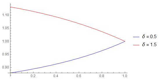
   (a) $\gamma=2$

   Figure 1. Graphs displaying the function $c(t)$ for different values of the parameters. In this case we have $\frac{\mathbb{E}[\rho(\delta-1)]}{1+\mathbb{E}[\theta(\delta-1)]}=0.4$, $\iota=0.2$.

2. The case $\gamma<1$ is symmetric: there exists $\delta^{*}\in\mathbb{R}$ such that for every $\delta\in(-\infty,\delta^{*})$, $c(t)$ is increasing, and decreasing if $\delta\in(\delta^{*},\infty)$.

Now observe that in the time-additive case of Lacker and Soret [19], $\lambda=1$. A typical empirical value for risk aversion is $\gamma=2$ (see the discussion in [14, p. 574]). It follows that implicitly in the time-additive model one assumes $\delta=1/2$. This might be very misleading as $\delta>1$ is a common assumption in asset pricing (e.g., see [2]). If we take $\delta>1$, it follows that $\lambda$ is negative, thus changing the shape of equilibrium consumption. In particular, Figure 1 illustrates this point: the function $c(t)$ can switch from increasing to decreasing depending on whether $\delta$ is smaller or greater than unity. Hence, under the framework of stochastic differential utility, it is possible to distinguish the effect of the elasticity of intertemporal substitution (EIS) from that of risk aversion on equilibrium consumption behavior, avoiding potentially misleading conclusions.

2.4. The Mean-Field Game as a Limit of Finite Player Games

In this subsection we discuss the relations between the MFG and the $N$-player game for large $N$. In order to simplify the discussion, we assume (with no further reference)

$$(x_{0}^{i},\mu_{i},\nu_{i},\sigma_{i},\eta_{i},\gamma_{i},\delta_{i},\epsilon_{i},\theta_{i})=(x_{0},\mu,\nu,\sigma,\eta,\gamma,\delta,\epsilon,\theta)\in\mathcal{I},\text{ for any $i=1,...,N$}.$$

In particular, notice that we are assuming the coefficients of the MFG to be deterministic.

We first state the following convergence result.

Theorem 2.8 (Convergence to the MFGE).

Let $\hat{\bm{\alpha}}_{N}=(\hat{c}_{i,N},\hat{\pi}_{i,N})_{i=1,...,N}$ be the simple NE equilibrium of the $N$-player game as in Theorem 2.2 and let $(\hat{c},\hat{\pi})$ be the simple MFGE as in Theorem 2.6, with corresponding $(\hat{m},\hat{Y})$. We have convergence of the equilibrium strategies

$$\sup_{t\in[0,T]}|\hat{c}_{i,N}(t)-\hat{c}(t)|+|\hat{\pi}_{i,N}-\hat{\pi}|=O(1/N),\text{ for any $i=1,...,N$,}$$

of the mean-field terms

$$\sup_{t\in[0,T]}|\log\overline{X}_{t}^{N}-\log\hat{Y}_{t}|=O\big{(}N^{-\frac{1}{2}}(\log N)^{-\frac{1}{2}-a}\big{)},\text{ $\mathbb{P}$-a.s.,}$$

$$\sup_{t\in[0,T]}|\overline{c}^{N}(t)-\hat{m}(t)|=O(1/N),$$

for any $a>0$, and of the values at equilibrium $|V^{i}_{0}(\hat{\bm{\alpha}}^{N})-V_{0}(\hat{\alpha},\hat{X},\hat{m})|=O(1/N),$ for any $i$.

We next show that the MFGE does indeed approximate NE of the corresponding game with finitely many players. In particular, we will use the MFGE $\hat{\alpha}=(\hat{c},\hat{\pi})$ in order to construct approximate NE for the original $N$-player game. For any $N\in\mathbb{N}_{0}$, define the strategy profile $\hat{\bm{\alpha}}_{N}^{\infty}$ in which all players are using the simple (deterministic) strategy $\hat{\alpha}$; that is,

$$\hat{\bm{\alpha}}_{N}^{\infty}:=(\hat{\alpha},...,\hat{\alpha})\in\mathcal{A}_{N}^{N}.$$

We have the following result.

Theorem 2.9 (Approximate NE).

The strategy profile $\hat{\bm{\alpha}}_{N}^{\infty}$ is an approximate NE of order $O(1/N)$ as $N\to\infty$; that is,

$$\big{|}V_{0}^{i}(\hat{\bm{\alpha}}_{N}^{\infty})-\sup_{\alpha_{i}\in\mathcal{A}_{N}}V_{0}^{i}(\alpha_{i},\hat{\bm{\alpha}}_{-i,N}^{\infty})\big{|}=O(1/N),$$

for any $i=1,...,N$.

3. Preliminary results on geometric-Bernoulli BSDEs

Observe that, given a profile $\bm{\alpha}$, for any $i=1,...,N$ the processes $X^{i},\,\overline{X}$ are generalized geometric Brownian motions, hence so it is $X^{i}(\overline{X})^{-\theta}$. Therefore, the system (5)-(6), is a forward backward stochastic differential equation in which the forward component is a geometric Brownian motion and in which the backward component has Bernoulli driver (i.e., $f(C,v)=f_{1}v+f_{2}(C)v^{q}$, for $q\geq 0$, $q\neq 0,1$). Since the forward components do not depend on the backward component, we will refer to such type of systems as geometric-Bernoulli BSDEs.

An essential tool in the proof of our main results are explicit solvability, stability and characterization of optimal controls when optimizing this type of systems. We devote this section to address this preliminary results.

3.1. Geometric-Bernoulli BSDEs

Let $(\tilde{\Omega},\tilde{\mathcal{F}},\tilde{\mathbb{F}}=(\tilde{\mathcal{F}}_{t})_{t\in[0,T]},\tilde{\mathbb{P}})$ be a generic filtered probability space satisfying the usual conditions, on which are defined independent $\tilde{\mathbb{F}}$-Brownian motions $\tilde{W}^{1},\tilde{W}^{2},B$. Let $(x_{0},\mu,\nu,\sigma,\eta,\gamma,\delta,\epsilon,\theta)$ be an $\tilde{\mathcal{F}}_{0}$-measurable $\mathcal{I}$-valued random variable satisfying (10) $\tilde{\mathbb{P}}$-a.s., and take deterministic functions $b^{2},\hat{b}^{2}:[0,T]\to[0,\infty)$ and parameters $\mu^{2}\in\mathbb{R},\ \nu^{2},\sigma^{2}\geq 0,y_{0}>0$. For $\gamma,\delta\neq 1$, $\lambda,q$ as in (10), $p,\theta\in[0,1]$, let the (random) aggregator $f:=f(\cdot;\eta,\delta,\gamma)$ and the terminal cost $g:=g(\cdot;\gamma,\epsilon)$ be as in (2).

A strategy $\alpha=(c,\pi)$ is a couple of $(0,\infty)\times\mathbb{R}$-valued $\tilde{\mathbb{F}}$-progressively measurable processes such the boundedness conditions in (3) are satisfied. The space of strategies is denoted by $\tilde{\mathcal{A}}$. Simple strategies such that $(c,\pi)$ is $\tilde{\mathcal{F}}_{0}$-measurable, with $\pi$ constant in time. Let $\alpha=(c,\pi)$ be a strategy, and consider the related solution $(X^{\alpha},Y,V^{\alpha},Z^{\alpha})$ of the geometric-Bernoulli BSDE

(16) $$dX^{\alpha}_{t} =\pi_{t}X^{\alpha}_{t}(\mu^{1}+\nu^{1}d\tilde{W}^{1}_{t}+\sigma^{1}dB_{t})-c_{t}X_{t}dt,\quad X^{\alpha}_{0}=x_{0},$$

$$dY_{t} =Y_{t}((\mu^{2}-\hat{b}_{t}^{2})dt+\nu^{2}d\tilde{W}^{2}_{t}+\sigma^{2}dB_{t}),\quad Y_{0}=y_{0},$$

$$dV_{t}^{\alpha} =-f((c_{t}X_{t})^{p}(b_{t}^{2}Y_{t})^{-\theta},V_{t}^{\alpha})dt+Z^{\alpha}_{t}d(\tilde{W}^{1},\tilde{W}^{2},B)_{t},\quad V_{T}^{\alpha}=g((X_{T})^{p}Y_{T}^{-\theta}),$$

For simple strategies, the solution of geometric-Bernoulli BSDEs is related to the solution of the Bernoulli ordinary differential equation (ODE, in short)

$$h^{\prime}+\varphi(t)h+\psi(t)h^{1-a}=0,\quad h(T)=1,$$

for a suitable parameter $a$ and suitable continuous functions $\varphi,\psi:[0,T]\to\mathbb{R}$. When $a\neq 1,0$, it is well known that the unique solution of the Bernoulli ODE is given by

(17) $$h_{a,\varphi,\psi}(t):=\Big{(}e^{a\int_{t}^{T}\varphi(r)dr}+a\int_{t}^{T}\psi(r)e^{a\int_{t}^{s}\varphi(r)dr}ds\Big{)}^{\frac{1}{a}},$$

that we write here for future reference.

3.2. Solvability of geometric-Bernoulli BSDEs

For a strategy $\alpha=(c,\pi)\in\tilde{\mathcal{A}}$, define the (random) coefficients

(18) $$\varphi_{t}^{\alpha} :=-\eta\lambda+(1-\gamma)\big{(}p(\pi_{t}\mu^{1}-c_{t})-\theta(\mu^{2}-\hat{b}_{t}^{2})+\frac{1}{2}p(p(1-\gamma)-1)\pi_{t}^{2}((\nu^{1})^{2}+(\sigma^{1})^{2})$$

$$\quad\quad\quad\quad\quad+\frac{1}{2}\theta(1+\theta(1-\gamma))((\nu^{2})^{2}+(\sigma^{2})^{2})-p\theta(1-\gamma)\pi_{t}\sigma^{1}\sigma^{2}\big{)},$$

$$\psi_{t}^{\alpha} :=\lambda\epsilon^{-1}\big{(}{c_{t}}^{p}{(b_{t}^{2})^{-\theta}}\big{)}^{1-\frac{1}{\delta}},$$

$$\beta_{t}^{\alpha} :=\big{(}p(1-\gamma)\pi_{t}\nu^{1},-\theta(1-\gamma)\nu^{2},(1-\gamma)(p\pi_{t}\sigma^{1}-\theta(1-\gamma)\sigma^{2})\big{)}.$$

We then discuss a first characterization result for $V^{\alpha}$.

Lemma 3.1.

The unique solution $(X^{\alpha},Y,V^{\alpha},Z^{\alpha})$ of the geometric-Bernoulli BSDE (16) has backward component $V^{\alpha}$ characterized by

$$V_{t}^{\alpha}=\frac{(\eta\epsilon)^{\lambda}}{1-\gamma}H^{\alpha}_{t}((X^{\alpha}_{t})^{p}Y_{t}^{-\theta})^{1-\gamma},$$

with $(H^{\alpha},N^{1,\alpha},N^{2,\alpha},\Sigma^{\alpha})$ solution to the BSDE

(19) $$dH_{t}= -\Psi^{\alpha}(t,H_{t},N^{1}_{t},N^{2}_{t},\Sigma_{t})dt+(N_{t}^{1},N_{t}^{2},\Sigma_{t})d(\tilde{W}^{1},\tilde{W}^{2},B)_{t},\quad H_{T}=1,$$

with driver $\Psi^{\alpha}(t,h,n^{1},n^{2},z):=\varphi_{t}^{\alpha}h+\psi_{t}^{\alpha}h^{1-\frac{1}{\lambda}}+\beta_{t}^{\alpha}(n^{1},n^{2},z)$ and $\varphi^{\alpha},\psi^{\alpha},\beta^{\alpha}$ defined in (18).

Proof.

In order to simplify the notation, we drop the superscript $\alpha$. The forward equations of (16) admits a unique solution (in explicit form) while the BSDE has a unique solution by Remark 2.4 (as $\tilde{\mathcal{F}}_{0}$ is not necessarily trivial). Thus, we define the process $H$ as $H_{t}:=\frac{1-\gamma}{(\eta\epsilon)^{\lambda}}V_{t}(X_{t}^{p}Y_{t}^{-\theta})^{\gamma-1}$ and we search for a BSDE representation of $H$.

By using the terminal condition for $V_{T}$, it is immediate to verify that $H_{T}=1$. Moreover, thanks to Itô formula we find

$$dH_{t}= -\big{[}\hat{\varphi}_{t}^{\alpha}H_{t}+\psi_{t}^{\alpha}H_{t}^{1-\frac{1}{\lambda}}$$

$$\quad+(1-\gamma)\frac{1-\gamma}{(\eta\epsilon)^{\lambda}}(X_{t}^{p}Y_{t}^{-\theta})^{\gamma-1}\big{(}p\pi_{t}(\nu^{1}Z_{t}^{1}+\sigma^{1}Z^{0}_{t})-\theta(\nu^{2}Z^{2}_{t}+\sigma^{2}Z^{0}_{t})\big{)}\big{]}dt$$

$$\quad+\frac{1-\gamma}{(\eta\epsilon)^{\lambda}}(X_{t}^{p}Y_{t}^{-\theta})^{\gamma-1}Z_{t}d(\tilde{W}^{1},\tilde{W}^{2},B)_{t}$$

$$\quad+(1-\gamma)H_{t}\big{(}-p(\pi_{t}\nu^{1}dW^{1}+\pi_{t}\sigma^{1}dB_{t})+\theta(\nu^{2}dW^{2}_{t}+\sigma^{2}dB_{t})\big{)},$$

where

$$\hat{\varphi}_{t}^{\alpha} :=-\eta\lambda+(1-\gamma)\big{(}p(\pi_{t}\mu^{1}-c_{t})-\theta(\mu^{2}-\hat{b}_{t}^{2})+\frac{1}{2}p(-p(1-\gamma)-1)\pi_{t}^{2}((\nu^{1})^{2}+(\sigma^{1})^{2})$$

$$\quad\quad\quad\quad\quad+\frac{1}{2}\theta(1-\theta(1-\gamma)))((\nu^{2})^{2}+(\sigma^{2})^{2})+p\theta(1-\gamma)\pi_{t}\sigma^{1}\sigma^{2}\big{)}.$$

Hence, defining

$$N^{1}_{t} :=-p(1-\gamma)H_{t}\pi_{t}\nu^{1}+\frac{1-\gamma}{(\eta\epsilon)^{\lambda}}(X_{t}^{p}Y_{t}^{-\theta})^{\gamma-1}Z^{1}_{t},$$

$$N^{2}_{t} :=\theta(1-\gamma)H_{t}\nu^{2}+\frac{1-\gamma}{(\eta\epsilon)^{\lambda}}(X_{t}^{p}Y_{t}^{-\theta})^{\gamma-1}Z^{2}_{t},$$

$$\Sigma_{t} :=-p(1-\gamma)H_{t}\pi_{t}\sigma^{1}+\theta(1-\gamma)H_{t}\sigma^{2}+\frac{1-\gamma}{(\eta\epsilon)^{\lambda}}(X_{t}^{p}Y_{t}^{-\theta})^{\gamma-1}Z^{0}_{t},$$

and substituting into the latter equation, we obtain

$$dH_{t}= -\big{[}\big{(}\hat{\varphi}_{t}^{\alpha}+p^{2}(1-\gamma)\pi_{t}^{2}((\nu^{1})^{2}+(\sigma^{1})^{2})+(1-\gamma)\theta^{2}((\nu^{2})^{2}+(\sigma^{2})^{2})$$

$$\quad-2p\theta(1-\gamma)\pi_{t}\sigma^{1}\sigma^{2}\big{)}H_{t}+\psi_{t}^{\alpha}H_{t}^{1-\frac{1}{\lambda}}+\beta_{t}^{\alpha}(N_{t}^{1},N_{t}^{2},\Sigma_{t})\big{]}dt$$

$$\quad+(N_{t}^{1},N_{t}^{2},\Sigma_{t})d(\tilde{W}^{1},\tilde{W}^{2},B)_{t}.$$

Finally, by the definitions of $\varphi^{\alpha}$ and of $\hat{\varphi}^{\alpha}$, we conclude that

$$dH_{t}= -\big{[}\varphi_{t}^{\alpha}H_{t}+\psi_{t}^{\alpha}H_{t}^{1-\frac{1}{\lambda}}+\beta_{t}^{\alpha}(N_{t}^{1},N_{t}^{2},\Sigma_{t})\big{]}dt+(N_{t}^{1},N_{t}^{2},\Sigma_{t})d(\tilde{W}^{1},\tilde{W}^{2},B)_{t},$$

which is the desired BSDE. ∎

When the considered strategy $\alpha$ is simple, a more elementary characterization of $V^{\alpha}$ can be given in terms of a (random) Bernoulli ODE. This representation also imply certain stability of the system and will be crucial when showing the convergence and approximation results (see the proofs of Theorems 2.8 and 2.9 in Section 4).

Lemma 3.2.

For a simple strategy $\alpha=(c,\pi)$, the unique solution $(X^{\alpha},Y,V^{\alpha},Z^{\alpha})$ of the geometric-Bernoulli BSDE (16) has backward component $V^{\alpha}$ characterized by

$$V^{\alpha}_{t}=\frac{(\eta\epsilon)^{\lambda}}{1-\gamma}h_{\frac{1}{\lambda},\varphi^{\alpha},\psi^{\alpha}}(t)((X_{t}^{\alpha})^{p}Y_{t}^{-\theta})^{1-\gamma},$$

with $\varphi^{\alpha},\psi^{\alpha}$ as in (18) and $h_{\frac{1}{\lambda},\varphi^{\alpha},\psi^{\alpha}}$ as in (17).

Proof.

Thanks to Lemma 3.1, $V^{\alpha}$ can be characterized in terms of the solution $H^{\alpha}$ of (19). Notice that if the strategy $\alpha$ is simple, then the parameters $\varphi^{\alpha},\psi^{\alpha}$ of (18) are $\tilde{\mathcal{F}}_{0}$-measurable. Hence, the BSDE (19) has $\tilde{\mathcal{F}}_{0}$-measurable coefficients as well as $\tilde{\mathcal{F}}_{0}$-measurable terminal condition. Therefore, its solution is $\tilde{\mathcal{F}}_{0}$-measurable (in particular, $N^{1,\alpha}=N^{2,\alpha}=\Sigma^{\alpha}=0$) and it coincides with the solution of the (random) Bernoulli ODE

$$dH_{t}=-[\varphi_{t}^{\alpha}H_{t}+\psi_{t}^{\alpha}H_{t}^{1-\frac{1}{\lambda}}]dt,\quad H_{T}=1,$$

which is given by $h_{\frac{1}{\lambda},\varphi^{\alpha},\psi^{\alpha}}$ as in (17). ∎

3.3. Optimizing against simple strategies

We next turn our focus on the optimization problem

(20) $$\operatorname*{Max}_{\alpha\in\tilde{\mathcal{A}}}V_{0}^{\alpha},$$

where $\tilde{\mathcal{A}}$ is the set of strategies and $(X^{\alpha},Y,V^{\alpha},Z^{\alpha})$ solves the system (16).

Hinging on the representation of Lemma 3.1, the next theorem characterizes explicitly the optimal controls and represents the starting point in order to derive the equilibria of the games (see the proofs of Theorems 2.2 and 2.6 in Section 4 below).

Theorem 3.3.

The control problem (20) admits an optimal simple control $(c^{*},\pi^{*})$ given by

(21) $$c^{*}_{t} :=c^{*}_{t}(\mu^{2},\hat{b}^{2},\nu^{2},\sigma^{2},b^{2};\mu^{1},\nu^{1},\sigma^{1},f,g,p):=\epsilon^{-a}(b^{2}_{t})^{-\theta(1-\frac{1}{\delta})a}\big{(}h_{\frac{a}{\lambda},\varphi^{*},\psi^{*}}(t)\big{)}^{-\frac{a}{\lambda}}$$

$$\pi^{*}_{t} :=\pi^{*}_{t}(\mu^{2},\hat{b}^{2},\nu^{2},\sigma^{2},b^{2};\mu^{1},\nu^{1},\sigma^{1},f,g,p):=\frac{\mu^{1}-\sigma^{1}\sigma^{2}\theta(1-\gamma)}{(1-p(1-\gamma))((\nu^{1})^{2}+(\sigma^{1})^{2})},$$

for functions

(22) $$\varphi^{*}(t) :=-\eta\lambda+(1-\gamma)\Big{[}-\theta(\mu^{2}-\hat{b}_{t}^{2})+\frac{1}{2}\theta(1+\theta(1-\gamma))((\nu^{2})^{2}+(\sigma^{2})^{2})$$

$$\quad\quad\quad\quad\quad\quad\quad\quad\quad-\frac{1}{2}p\frac{(\sigma^{1}\sigma^{2}\theta(1-\gamma)-\mu^{1})^{2}}{(p(1-\gamma)-1)((\nu^{1})^{2}+(\sigma^{1})^{2})}\Big{]},$$

$$\psi^{*}(t) :=\epsilon^{-a}(\lambda-p(1-\gamma))(b_{t}^{2})^{-\theta(1-\frac{1}{\delta})a},$$

and for $a:=(1-p(1-\frac{1}{\delta}))^{-1}$.

Proof.

The proof hinges on the representation of Lemma 3.1 and on a comparison theorem for BSDEs. Notice indeed that, thanks to Lemma 3.1, the optimal control problem $\max_{\alpha}V_{0}^{\alpha}$ is equivalent to the maximization problem $\max_{\alpha}\frac{H_{0}^{\alpha}}{1-\gamma}$. Hence, the optimization problem depends on the sign of $1-\gamma$, and becomes a minimization problem if $1-\gamma<0$. We limit our self to show the case in which $1-\gamma>0$, the case $1-\gamma<0$ is analoguous.

We divide the rest of the proof in two steps.

Step 1. We first consider the solution to the BSDE (19) with maximal driver. Namely, $\Psi^{\alpha}$ as in Lemma 3.1, define

$$\Psi^{*}(t,h,n^{1},n^{2},z):=\sup_{\alpha\in\tilde{\mathcal{A}}}\Psi^{\alpha}(t,h,n^{1},n^{2},z),$$

and observe that the $\tilde{\alpha}=(\tilde{c},\tilde{\pi})$ attaining the supremum writes as a functions of $(t,h,n^{1},n^{2},z)$ as

(23) $$\tilde{c}(t,h,n^{1},n^{2},z) :=\epsilon^{-a}(b^{2}_{t})^{-a\theta(1-\frac{1}{\delta})}h^{-\frac{a}{\lambda}}$$

$$\tilde{\pi}(t,h,n^{1},n^{2},z) :=\frac{\mu^{1}+\nu^{1}\frac{n^{1}}{h}+\sigma^{1}\frac{z}{h}-\sigma^{1}\sigma^{2}\theta(1-\gamma)}{(1-p(1-\gamma))((\nu^{1})^{2}+(\sigma^{1})^{2})}.$$

Moreover, $\Psi^{*}$ writes as

$$\Psi^{*}(t,h,n^{1},n^{2},z)=\tilde{\varphi}^{*}(t,h,n^{1},n^{2},z)h+\tilde{\psi}^{*}(t,h,n^{1},n^{2},z)h^{1-\frac{a}{\lambda}}$$

where we define

(24) $$\tilde{\varphi}^{*}(t,h,n^{1},n^{2},z) :=-\eta\lambda+(1-\gamma)\Big{[}-\theta(\mu^{2}-\hat{b}_{t}^{2})+\frac{1}{2}\theta(1+\theta(1-\gamma))((\nu^{2})^{2}+(\sigma^{2})^{2})$$

$$\quad\quad\quad\quad\quad\quad\quad\quad\quad-\theta\nu^{2}\frac{n^{2}}{h}-\theta\sigma^{2}\frac{z}{h}$$

$$\quad\quad\quad\quad\quad\quad\quad\quad\quad-\frac{1}{2}p\frac{(\mu^{1}+\nu^{1}\frac{n^{1}}{h}+\sigma^{1}\frac{z}{h}-\sigma^{1}\sigma^{2}\theta(1-\gamma))^{2}}{(p(1-\gamma)-1)((\nu^{1})^{2}+(\sigma^{1})^{2})}\Big{]},$$

$$\tilde{\psi}^{*}(t,h,n^{1},n^{2},z) :=\epsilon^{-a}(\lambda-p(1-\gamma))(b_{t}^{2})^{-a\theta(1-\frac{1}{\delta})}.$$

Consider now the BSDE

(25) $$dH_{t}=-\Psi^{*}(t,H_{t},N^{1}_{t},N^{2}_{t},\Sigma_{t})dt+(N_{t}^{1},N_{t}^{2},\Sigma_{t})d(\tilde{W}^{1},\tilde{W}^{2},B)_{t},\quad H_{T}=1.$$

Since the coefficients of $\Psi^{*}$ and the terminal condition are $\tilde{\mathcal{F}}_{0}$-measurable, we search for a $\tilde{\mathcal{F}}_{0}$-measurable solution $(H^{*},N^{1,*},N^{2,*},\Sigma^{*})$, with $N^{1,*}=N^{2,*}=\Sigma^{*}=0$. Then, for $\varphi^{*}_{t},\psi^{*}_{t}$ as in (22), the previous BSDE writes as

$$dH_{t}=-\Psi^{*}(t,H_{t},0,0,0)dt=-(\varphi^{*}_{t}H_{t}+\psi^{*}_{t}H^{1-\frac{a}{\lambda}})dt,\quad H_{T}=1,$$

which is a Bernoulli ODE with solution $H^{*}:=h_{\frac{a}{\lambda},\varphi^{*},\psi^{*}}$ (cf. (17)).

Step 2. We now want to show that $H^{*}_{0}\geq H^{\alpha}_{0}$ for any strategy $\alpha$. To this end, we will make a logarithmic change of variable and then use a comparison principle for quadratic BSDEs.

Define the transformation $(\tilde{h},\tilde{n}^{1},\tilde{n}^{2},\tilde{z}):=F(h,n^{1},n^{2},z):=(\log h,n^{1}/h,n^{2}/h,z/h)$. For $H^{*}$ as in the previous step, the process $(\tilde{H},\tilde{N}^{1},\tilde{N}^{2},\tilde{\Sigma}):=F(H^{*},0,0,0)$ solves the BSDE

$$d\tilde{H}_{t}=-\tilde{\Psi}^{*}(t,\tilde{H}_{t},\tilde{N}^{1}_{t},\tilde{N}^{2}_{t},\tilde{\Sigma}_{t})dt+(\tilde{N}_{t}^{1},\tilde{N}_{t}^{2},\tilde{\Sigma}_{t})d(\tilde{W}^{1},\tilde{W}^{2},B)_{t},\quad\tilde{H}_{T}=0,$$

where the new driver $\tilde{\Psi}^{*}$ is defined as

$$\tilde{\Psi}^{*}(t,\tilde{h},\tilde{n}^{1},\tilde{n}^{2},\tilde{z}):=\varphi^{*}(t,\tilde{h},\tilde{n}^{1},\tilde{n}^{2},\tilde{z})+\psi^{*}(t,\tilde{h},\tilde{n}^{1},\tilde{n}^{2},\tilde{z})e^{-\frac{a}{\lambda}\tilde{h}}+\frac{1}{2}|(\tilde{n}^{1},\tilde{n}^{2},\tilde{z})|^{2}.$$

Similarly, for generic $\alpha\in\tilde{\mathcal{A}}$ and $(H^{\alpha},N^{1,\alpha},N^{2,\alpha},\Sigma^{\alpha})$ solution to (19), the process $(\tilde{H}^{\alpha},\tilde{N}^{1,\alpha},\tilde{N}^{2,\alpha},\tilde{\Sigma}^{\alpha}):=F(H^{\alpha},N^{1,\alpha},N^{2,\alpha},\Sigma^{\alpha})$ solves the BSDE

$$d\tilde{H}_{t}=-\tilde{\Psi}^{\alpha}(t,\tilde{H}_{t},\tilde{N}^{1}_{t},\tilde{N}^{2}_{t},\tilde{\Sigma}_{t})dt+(\tilde{N}_{t}^{1},\tilde{N}_{t}^{2},\tilde{\Sigma}_{t})d(\tilde{W}^{1},\tilde{W}^{2},B)_{t},\quad\tilde{H}_{T}=0,$$

where the new driver $\tilde{\Psi}^{\alpha}$ is defined as

$$\tilde{\Psi}^{\alpha}(t,\tilde{h},\tilde{n}^{1},\tilde{n}^{2},\tilde{z}):= \varphi^{\alpha}_{t}+\psi^{\alpha}_{t}e^{-\frac{1}{\lambda}\tilde{h}}+\beta^{\alpha}_{t}(\tilde{n}^{1},\tilde{n}^{2},\tilde{z})+\frac{1}{2}|(\tilde{n}^{1},\tilde{n}^{2},\tilde{z})|^{2}.$$

Now, the reader can easily verify that $\tilde{\Psi}^{*}(t,\tilde{h},\tilde{n}^{1},\tilde{n}^{2},\tilde{z})\geq\tilde{\Psi}^{\alpha}(t,\tilde{h},\tilde{n}^{1},\tilde{n}^{2},\tilde{z})$ for any $\alpha\in\tilde{\mathcal{A}}$. Therefore, Theorem 2.6 in [16] implies that $\tilde{H}_{0}^{*}\geq\tilde{H}_{0}^{\alpha}$, which in turn gives $H_{0}^{*}=e^{\tilde{H}_{0}^{*}}\geq e^{\tilde{H}_{0}^{\alpha}}=H_{0}^{\alpha}$, thus completing the proof in the case $1-\gamma>0$. ∎

4. Proof of the Main Theorems

4.1. Proof of Theorem 2.2

We search for NE involving simple strategies. The rest of the proof is divided into two steps.

Step 1. In this step we determine the optimal control for the optimization problem of player $i$ in response to simple strategies $(c_{j},\pi_{j})_{j\neq i}$ chosen by its opponent.

First of all, observe that, if the opponents of player $i$ choose simple strategies $(c_{j},\pi_{j})_{j\neq i}$, then the process

$$Y^{i}_{t} :=\Big{(}\prod_{j\neq i}X^{j}_{t}\Big{)}^{\frac{1}{N}}$$

$$=\Big{(}\prod_{j\neq i}x^{j}_{0}\Big{)}^{\frac{1}{N}}\exp\Big{[}\frac{1}{N}\sum_{j\neq i}\Big{(}\big{(}\pi_{j}\mu_{j}-\frac{1}{2}\pi_{j}^{2}(\nu_{j}^{2}+\sigma_{j}^{2})\big{)}t-\int_{0}^{t}c_{j}(s)ds+\pi_{j}\nu_{j}W^{j}_{t}+\pi_{j}\sigma_{j}B_{t}\Big{)}\Big{]}$$

is an generalized geometric Brownian motion. In particular, we can write

$$dY^{i}_{t}=Y^{i}_{t}((\hat{\mu}_{i}-\hat{b}_{i}(t))dt+\hat{\nu}_{i}d\hat{W}^{i}_{t}+\hat{\sigma}_{i}dB_{t}),\quad Y^{i}_{0}=y^{i}_{0},$$

where the new parameters are defined by

(26) $$y^{i}_{0} :=\Big{(}\prod_{j\neq i}x^{j}_{0}\Big{)}^{\frac{1}{N}},\quad\hat{\nu}_{i}:=\frac{1}{N}\sqrt{\sum_{j\neq i}(\pi_{j}\nu_{j})^{2}},\quad\hat{\sigma}_{i}:=\frac{1}{N}\sum_{j\neq i}\pi_{j}\sigma_{j},$$

$$\hat{\mu}_{i} :=\frac{1}{N}\sum_{j\neq i}\big{(}\pi_{j}\mu_{j}-\frac{1}{2}\pi_{j}^{2}(\nu_{j}^{2}+\sigma_{j}^{2})\big{)}+\frac{1}{2}(\hat{\nu}_{i}^{2}+\hat{\sigma}_{i}^{2}),$$

$$\hat{b}_{i}(t) :=\frac{1}{N}\sum_{j\neq i}c_{j}(t),\quad\hat{W}^{i}_{t}:=\frac{1}{\sqrt{\sum_{j\neq i}(\pi_{j}\nu_{j})^{2}}}\sum_{j\neq i}\pi_{j}\nu_{j}W^{j}_{t}.$$

Moreover, the process $\hat{W}^{i}$ is a Brownian motion independent from $W^{i}$ and $B$. Thus, set

$$\bar{b}_{i}(t):=\Big{(}\prod_{j\neq i}c_{j}(t)\Big{)}^{\frac{1}{N}},$$

and observe that the control problem of player $i$ is given by $\operatorname*{Max}_{\alpha_{i}}V^{i}_{0}$, subject to

$$dX^{i}_{t} =\pi^{i}_{t}X^{i}_{t}(\mu_{i}dt+\nu_{i}dW^{i}_{t}+\sigma_{i}dB_{t})-c_{i}(t)X^{i}_{t}dt,\quad X^{i}_{0}=x^{i}_{0},$$

$$dY^{i}_{t} =Y^{i}_{t}((\hat{\mu}_{i}-\hat{b}_{i}(t))dt+\hat{\nu}_{i}d\hat{W}^{i}_{t}+\hat{\sigma}_{i}dB_{t}),\quad Y^{i}_{0}=y^{i}_{0},$$

$$dV^{i}_{t} =-f_{i}((c_{i}(t)X^{i}_{t})^{1-\frac{\theta}{N}}(\bar{b}_{i}(t)Y^{i}_{t})^{-\theta},V^{i}_{t})dt+Z^{i}_{t}d(W^{i},\hat{W}^{i},B)_{t},\ V^{i}_{T}=g_{i}((X^{i}_{T})^{1-\frac{\theta}{N}}(Y^{i}_{T})^{-\theta}).$$

Since such a control problem is (for suitable choice of parameters) of type (20), we can use Theorem 3.3 in order to find the best response $(c_{i}^{*},\pi_{i}^{*})$ to the strategies $(c_{j},\pi_{j})_{j\neq i}$:

(27) $${c}_{i}^{*}(t) :={c}_{t}^{*}(\hat{\mu}_{i},\hat{b}_{i},\hat{\nu}_{i},\hat{\sigma}_{i},\bar{b}_{i};\mu_{i},\nu_{i},\sigma_{i},f_{i},g_{i},1-{\theta_{i}}/{N}),$$

$${\pi}_{i}^{*}(t) :={\pi}^{*}_{t}(\hat{\mu}_{i},\hat{b}_{i},\hat{\nu}_{i},\hat{\sigma}_{i},\bar{b}_{i};\mu_{i},\nu_{i},\sigma_{i},f_{i},g_{i},1-{\theta_{i}}/{N}),$$

where the maps ${c}_{t}^{*}$ and $\pi_{t}^{*}$ are defined in (21) and the parameters are defined in (26).

Step 2. In this step we search for a NE $(\bm{c},\bm{\pi})=((c_{1},\pi_{1}),...,(c_{N},\pi_{N}))$ of the game. The argument is adapted from [19]. Observe that, in light of (27), the simple strategy profile $(\bm{c},\bm{\pi})$ is a NE of the game if and only if it satisfies the fixed point condition

$${c}_{i}(t) =c^{*}_{t}(\hat{\mu}_{i},\hat{b}_{i},\hat{\nu}_{i},\hat{\sigma}_{i},\bar{b}_{i};\mu_{i},\nu_{i},\sigma_{i},f_{i},g_{i},1-{\theta_{i}}/{N}),$$

$${\pi}_{i} =\pi^{*}_{t}(\hat{\mu}_{i},\hat{b}_{i},\hat{\nu}_{i},\hat{\sigma}_{i},\bar{b}_{i};\mu_{i},\nu_{i},\sigma_{i},f_{i},g_{i},1-{\theta_{i}}/{N}),$$

where the parameters in the right hand sides are given in (26) as function of $(\bm{c},\bm{\pi})$.

We first solve the fixed point for $\bm{\pi}$. Setting $\Pi:=\sum_{j=1}^{N}\sigma_{j}\pi_{j}$, the system of equations for $\pi_{j}$ rewrites as

$$\pi_{i}=\frac{\mu_{i}-\sigma_{i}\theta_{i}(1-\gamma_{i})\frac{1}{N}(\Pi-\sigma_{i}\pi_{i})}{(1-(1-\frac{\theta_{i}}{N})(1-\gamma_{i}))(\nu_{i}^{2}+\sigma_{i}^{2})},\quad i=1,...,N.$$

Since $(1-(1-\frac{\theta_{i}}{N})(1-\gamma_{i}))(\nu_{i}^{2}+\sigma_{i}^{2})-\sigma_{i}^{2}\frac{\theta_{i}}{N}(1-\gamma_{i})\neq 0$ (by our conditions on $\gamma_{i},\theta_{i},\nu_{i},\sigma_{i}$), solving for $\pi_{i}$ we obtain

(28) $$\pi_{i}=\frac{N\mu_{i}-{\sigma_{i}}\theta_{i}(1-\gamma_{i})\Pi}{N(1-(1-\frac{\theta_{i}}{N})(1-\gamma_{i}))(\nu_{i}^{2}+\sigma_{i}^{2})-\sigma_{i}^{2}\theta_{i}(1-\gamma_{i})},$$

so that, multiplying by $\sigma_{i}$ and summing over $i$, gives the equation

$$\Pi= \sum_{i=1}^{N}\frac{N\sigma_{i}\mu_{i}}{N(1-(1-\frac{\theta_{i}}{N})(1-\gamma_{i}))(\nu_{i}^{2}+\sigma_{i}^{2})-\sigma_{i}^{2}\theta_{i}(1-\gamma_{i})}$$

$$-\Pi\sum_{i=1}^{N}\frac{{\sigma_{i}^{2}}\theta_{i}(1-\gamma_{i})}{N(1-(1-\frac{\theta_{i}}{N})(1-\gamma_{i}))(\nu_{i}^{2}+\sigma_{i}^{2})-\sigma_{i}^{2}\theta_{i}(1-\gamma_{i})}.$$

By our conditions on $\gamma_{i},\theta_{i},\nu_{i},\sigma_{i}$, we have

$$1\neq-\sum_{i=1}^{N}\frac{{\sigma_{i}^{2}}\theta_{i}(1-\gamma_{i})}{N(1-(1-\frac{\theta_{i}}{N})(1-\gamma_{i}))(\nu_{i}^{2}+\sigma_{i}^{2})-\sigma_{i}^{2}\theta_{i}(1-\gamma_{i})},$$

so that the previous equation is uniquely solved by

$$\Pi= \frac{\sum_{i=1}^{N}\frac{N\sigma_{i}\mu_{i}}{N(1-(1-\frac{\theta_{i}}{N})(1-\gamma_{i}))(\nu_{i}^{2}+\sigma_{i}^{2})-\sigma_{i}^{2}\theta_{i}(1-\gamma_{i})}}{1+\sum_{i=1}^{N}\frac{{\sigma_{i}^{2}}\theta_{i}(1-\gamma_{i})}{N(1-(1-\frac{\theta_{i}}{N})(1-\gamma_{i}))(\nu_{i}^{2}+\sigma_{i}^{2})-\sigma_{i}^{2}\theta_{i}(1-\gamma_{i})}}.$$

Plugging the latter expression into (28), we obtain (after minimal computations) the formula for $\pi_{i}$ as in the thesis of the theorem.

We now solve the fixed point for $\bm{c}$. Due to (27) (written in terms of (21)) with parameters in (26), this means to solve the system of equations

(29) $${c}_{i}(t)= \epsilon_{i}^{-a_{i}}\bar{b}_{i}(t)^{-{\theta_{i}(1-\frac{1}{\delta_{i}})a_{i}}}h_{i}(t)^{-\frac{a_{i}}{\lambda_{i}}},$$

$$h_{i}^{\prime}= -\big{(}\rho_{i}+\theta_{i}(1-\gamma_{i})\hat{b}_{i}(t)\big{)}h_{i}$$

$$-\Big{(}\epsilon_{i}^{-a_{i}}\big{(}\lambda_{i}-\big{(}1-\frac{\theta_{i}}{N}\big{)}(1-\gamma_{i})\big{)}\bar{b}_{i}(t)^{-{\theta_{i}(1-\frac{1}{\delta_{i}})a_{i}}}\Big{)}h_{i}^{1-\frac{a_{i}}{\lambda_{i}}},$$

for $a_{i}:=\frac{1}{1-(1-\theta_{i}/n)(1-1/{\delta_{i}})}$ and where the parameter $\rho_{i}$ is defined as

$$\rho_{i} :=-\eta_{i}\lambda_{i}+(1-\gamma_{i})\Big{[}-\theta_{i}\hat{\mu}_{i}+\frac{1}{2}\theta_{i}(1+\theta_{i}(1-\gamma_{i}))(\hat{\nu}_{i}^{2}+\hat{\sigma}_{i}^{2})$$

$$\quad\quad\quad\quad\quad\quad\quad\quad\quad-\frac{1}{2}(1-\frac{\theta_{i}}{N})\frac{(\sigma_{i}\hat{\sigma}_{i}\theta_{i}(1-\gamma_{i})-\mu_{i})^{2}}{((1-\frac{\theta_{i}}{N})(1-\gamma_{i})-1)(\nu_{i}^{2}+\sigma_{i}^{2})}\Big{]}$$

has already been determined (by the fixed point in $\bm{\pi}$).

The first equation in (29) provides an expression for $h_{i}(t)^{-\frac{a_{i}}{\lambda_{i}}}$, which can be plugged into the second equation in (29) in order to obtain

$$h_{i}^{\prime}+\big{(}\rho_{i}+\theta_{i}(1-\gamma_{i})\hat{b}_{i}(t)+\big{(}\lambda_{i}-\big{(}1-\frac{\theta_{i}}{N}\big{)}(1-\gamma_{i})\big{)}c_{i}(t)\big{)}h_{i}=0,$$

which can be rewritten in terms of $\hat{b}(t):=\frac{1}{N}\sum_{i=1}^{N}c_{i}(t)$ as

$$h_{i}^{\prime}+\big{(}\rho_{i}+\theta_{i}(1-\gamma_{i})\hat{b}(t)+(\lambda_{i}-(1-\gamma_{i}))c_{i}(t)\big{)}h_{i}=0.$$

The latter differential equation, together with the terminal condition $h_{i}(T)=1$, can be solved in $h_{i}$ giving

$$h_{i}(t)=\exp\Big{(}\int_{t}^{T}\big{(}\rho_{i}+\theta_{i}(1-\gamma_{i})\hat{b}(s)+(\lambda_{i}-(1-\gamma_{i}))c_{i}(s)\big{)}ds\Big{)}.$$

Moreover, after some manipulation, the first equation in (29) can be rewritten in terms of $\bar{b}(t):=\frac{1}{N}\sum_{i=1}^{N}c_{i}(t)$ as

$$h_{i}(t)=\epsilon_{i}^{-\lambda_{i}}c_{i}(t)^{-\frac{\lambda_{i}}{\delta_{i}}}\bar{b}(t)^{-\lambda_{i}\theta_{i}(1-\frac{1}{\delta_{i}})},$$

which plugged into the latter equation gives

$$c_{i}(t)=\epsilon_{i}^{-\delta_{i}}\bar{b}(t)^{-\theta_{i}(\delta_{i}-1)}\exp\Big{(}-\frac{\delta_{i}}{\lambda_{i}}\int_{t}^{T}\big{(}\rho_{i}+\theta_{i}(1-\gamma_{i})\hat{b}(s)+(\lambda_{i}-(1-\gamma_{i}))c_{i}(s)\big{)}ds\Big{)},$$

or, equivalently,

(30) $$c_{i}(t)\exp\Big{(}\int_{t}^{T}c_{i}(s)ds\Big{)}=\epsilon_{i}^{-\delta_{i}}e^{-\frac{\delta_{i}}{\lambda_{i}}\rho_{i}(T-t)}\Big{(}\bar{b}(t)\exp\Big{(}\int_{t}^{T}\hat{b}(s)ds\Big{)}\Big{)}^{\theta_{i}(1-\delta_{i})}.$$

Thus, taking the geometric average over indexes $i=1,...,N$, we have

$$\bar{b}(t)\exp\Big{(}\int_{t}^{T}\hat{b}(s)ds\Big{)}=\kappa e^{-K(T-t)}\Big{(}\bar{b}(t)\exp\Big{(}\int_{t}^{T}\hat{b}(s)ds\Big{)}\Big{)}^{\frac{1}{N}\sum_{i=1}^{N}\theta_{i}(1-\delta_{i})}.$$

where

$$\kappa:=\Big{(}\prod_{i=1}^{N}\epsilon_{i}^{-\delta_{i}}\Big{)}^{\frac{1}{N}},\quad K:=\frac{1}{N}\sum_{i=1}^{N}\frac{\delta_{i}}{\lambda_{i}}\rho_{i}.$$

Therefore, since $\hat{q}:=1-\frac{1}{N}\sum_{i=1}^{N}\theta_{i}(1-\delta_{i})\neq 0$ by assumption, we obtain

(31) $$\bar{b}(t)\exp\Big{(}\int_{t}^{T}\hat{b}(s)ds\Big{)}=\kappa^{1/\hat{q}}e^{-\frac{K}{\hat{q}}(T-t)}.$$

Set now

$$\chi_{1}^{i}:=\epsilon_{i}^{-\delta_{i}}\kappa^{\frac{\theta_{i}(1-\delta_{i})}{\hat{q}}}\quad\text{and}\quad\chi_{2}^{i}:=-\frac{\delta_{i}}{\lambda_{i}}\rho_{i}-\theta_{i}(1-\delta_{i})\frac{K}{\hat{q}},$$

plug (31) into (30) in order to obtain

$$c_{i}(t)\exp\Big{(}\int_{t}^{T}c_{i}(s)ds\Big{)}=\chi_{1}^{i}e^{\chi_{2}^{i}(T-t)}.$$

Integrating and then computing the logarithm, we obtain

$$\int_{t}^{T}c_{i}(s)ds=\begin{cases}\log\big{[}1+\frac{\chi_{1}^{i}}{\chi_{2}^{i}}(e^{\chi_{2}^{i}(T-t)}-1)\big{]},&\text{ if }\chi_{2}^{i}\neq 0,\\ \log[\chi_{1}^{i}(T-t)+1],&\text{ if }\chi_{2}^{i}=0.\end{cases}$$

Finally, taking the derivative, we have

$$c_{i}(t)=\begin{cases}\Big{(}\frac{1}{{\chi_{2}^{i}}}+\big{(}\frac{1}{\chi_{1}^{i}}-\frac{1}{\chi_{2}^{i}}\big{)}e^{-\chi_{2}^{i}(T-t)}\Big{)}^{-1}&\text{ if }\chi_{2}^{i}\neq 0,\\ \big{(}T-t+\frac{1}{\chi_{1}^{i}}\big{)}^{-1}&\text{ if }\chi_{2}^{i}=0,\end{cases}$$

thus completing the proof of the theorem.

4.2. Proof of Theorem 2.6

The proof is similar to the proof of Theorem 2.2, we provide a sketch for the sake of completeness.

We first write the parameters of the control problem of the representative player, optimizing against a population of players using a simple (thus, $\mathcal{F}_{0}$-measurable) strategy $\alpha=(c,\pi)$. Indeed, the resulting state equation is given by

$$dY_{t}=Y_{t}((\hat{\mu}-\hat{b}(t))dt+\hat{\sigma}dB_{t}),\quad Y_{0}=y_{0},$$

where the new parameters are defined by

(32) $$y_{0} :=\exp(\mathbb{E}[\log x_{0}]),\quad\hat{\nu}:=0,\quad\hat{\sigma}:=\mathbb{E}[\pi\sigma],$$

$$\hat{\mu} :=\mathbb{E}[\pi\mu]-\frac{1}{2}\big{(}\mathbb{E}[\pi^{2}(\nu^{2}+\sigma^{2})]-(\mathbb{E}[\pi\sigma])^{2}\big{)},$$

$$\hat{b}_{t} :=\mathbb{E}[c_{t}],\quad\bar{b}_{t}:=\exp(\mathbb{E}[\log c_{t}]).$$

Thus, the control problem of the representative player is given by $\operatorname*{Max}_{\alpha}V_{0}$, subject to

$$dX_{t} =\pi_{t}X_{t}(\mu dt+\nu dW_{t}+\sigma dB_{t})-c(t)X_{t}dt,\quad X_{0}=x_{0},$$

$$dY_{t} =Y_{t}((\hat{\mu}-\hat{b}(t))dt+\hat{\sigma}dB_{t}),\quad Y_{0}=y_{0},$$

$$dV_{t} =-f(c(t)X_{t}(\bar{b}(t)Y_{t})^{-\theta},V_{t})dt+Z_{t}d(W,B)_{t},\ V_{T}=g(X_{T}Y_{T}^{-\theta}),$$

which is of type (20). Thanks to Theorem 3.3, the MFGE $(c,\pi)$ satisfies the relation:

(33) $${c}(t) :={c}_{t}^{*}(\hat{\mu},\hat{b},0,\hat{\sigma},\bar{b};\mu,\nu,\sigma,f,g,1),$$

$${\pi}(t) :={\pi}^{*}_{t}(\hat{\mu},\hat{b},0,\hat{\sigma},\bar{b};\mu,\nu,\sigma,f,g,1),$$

where the maps ${c}_{t}^{*}$ and $\pi_{t}^{*}$ are defined in (21) and the parameters are defined in (32).

We then search for a fixed point. Solving for $\pi$ first, we easily obtain

$$\pi=\frac{\mu}{\gamma(\sigma^{2}+\nu^{2})}-\theta\frac{1-\gamma}{\gamma}\frac{\sigma}{(\sigma^{2}+\nu^{2})}\left[\frac{\mathbb{E}\left[\frac{\mu\sigma}{\gamma(\sigma^{2}+\nu^{2})}\right]}{1+\mathbb{E}\left[\theta(\frac{1}{\gamma}-1)(\frac{\sigma^{2}}{\sigma^{2}+\nu^{2}})\right]}\right].$$

We next solve for $c$. By using (21), we write the system

(34) $${c}(t)= \epsilon^{-\delta}\bar{b}(t)^{\theta(1-\delta)}h(t)^{-\frac{\delta}{\lambda}},$$

$$h^{\prime}= -\big{(}\rho+\theta(1-\gamma)\hat{b}(t)\big{)}h-\big{(}\epsilon^{-\delta}\frac{\lambda}{\delta}\bar{b}(t)^{\theta(1-\delta)}\big{)}h^{1-\frac{\delta}{\lambda}},$$

where the parameter

$$\rho :=-\eta\lambda+(1-\gamma)\Big{[}-\theta\hat{\mu}+\frac{1}{2}\theta(1+\theta(1-\gamma))\hat{\sigma}^{2}+\frac{1}{2}\frac{(\sigma\hat{\sigma}\theta(1-\gamma)-\mu)^{2}}{\gamma(\nu^{2}+\sigma^{2})}\Big{]}$$

has already been determined (by the fixed point in $\pi$). Solving the first equation in (34) for $h(t)^{-\frac{\delta}{\lambda}}$, then plugging into the second equation and integrating the resulting differential equation, we obtain

$$h(t)=\exp\Big{(}\int_{t}^{T}\big{(}\rho+\theta(1-\gamma)\hat{b}(s)+\frac{\lambda}{\delta}c(s)\big{)}ds\Big{)}.$$

Sobstituting back into the first equation in (34), we obtain

$$c(t)\exp\Big{(}\int_{t}^{T}c(s)ds\Big{)}=\epsilon^{-\delta}e^{-\frac{\delta}{\lambda}\rho(T-t)}\exp\Big{(}\theta(1-\delta)\big{(}\mathbb{E}[\log c_{t}]+\int_{t}^{T}\mathbb{E}[c_{s}]ds\big{)}\Big{)}.$$

Taking expectations, we can solve for $\mathbb{E}[\log c_{t}]+\int_{t}^{T}\mathbb{E}[c_{s}]ds$, from which we obtain

$$c(t)\exp\Big{(}\int_{t}^{T}c(s)ds\Big{)}=\chi_{1}e^{-\chi_{2}(T-t)},$$

with

$$\chi_{1} :=\epsilon^{-\delta}\exp\Big{(}\frac{\theta(1-\delta)}{1-\mathbb{E}[\theta(1-\delta)]}\mathbb{E}[-\delta\log\epsilon]\Big{)},$$

$$\chi_{2} :=\frac{\delta}{\lambda}\rho+\frac{\theta(1-\delta)}{1-\mathbb{E}[\theta(1-\delta)]}\mathbb{E}\big{[}\frac{\delta}{\lambda}\rho\big{]},$$

Integrating the latter equation, then computing the logarithm and then taking the derivative, we have

$$c_{t}=\begin{cases}\Big{(}\big{(}\frac{1}{\chi_{1}}+\frac{1}{\chi_{2}}\big{)}e^{\chi_{2}(T-t)}-\frac{1}{{\chi_{2}}}\Big{)}^{-1}&\text{ if }\chi_{2}\neq 0,\\ \big{(}T-t+\frac{1}{\chi_{1}}\big{)}^{-1}&\text{ if }\chi_{2}=0,\end{cases}$$

thus completing the proof of the theorem.

4.3. Proof of Theorem 2.8

We divide the proof in two steps.

Step 1. We first study the convergence of the equilibrium strategies and of the mean field terms.

Using the explicit expressions derived in Theorems 2.2 and 2.6, elementary computations show that

(35) $$|\hat{\pi}_{i,N}-\hat{\pi}|=O(1/N).$$

Moreover, in the symmetric case we have

$$\chi_{1}^{i,N}=\chi_{1},\quad\text{for any $i$ and $N$,}$$

and, using (35), one obtains $|\rho_{i,N}-\rho|=O(1/N)$, which in turn gives

$$|\chi_{2}^{i,N}-\chi_{2}|=O(1/N),\quad\text{for any $i$ and $N$.}$$

Thus, from the latter two equations we conclude that

(36) $$\sup_{t\in[0,T]}|\hat{c}_{i,N}(t)-\hat{c}(t)|=O(1/N).$$

Furthermore, since $\hat{c}$ is deterministic we have $\hat{m}_{t}=\hat{c}_{t}$ and. since $\hat{c}_{i,N}$ does not depend on $i$ and it is deterministic, we obtain

$$\sup_{t\in[0,T]}|\bar{c}^{N}(t)-\hat{m}(t)|=O(1/N).$$

Next, for generic $i$ we can write

$$\overline{X}^{N}_{t}=x_{0}\exp\Big{(}\big{(}\hat{\pi}_{i,N}\mu-\frac{1}{2}\hat{\pi}_{i,N}^{2}(\nu^{2}+\sigma^{2})\big{)}t-\int_{0}^{t}\hat{c}_{i,N}(s)ds+\nu\hat{\pi}_{i,N}\frac{1}{N}\sum_{j=1}^{N}W^{j}_{t}+\hat{\pi}_{i,N}\sigma B_{t}\Big{)},$$

as well as

$$\hat{Y}_{t}=x_{0}\exp\Big{(}\big{(}\hat{\pi}\mu-\frac{1}{2}\hat{\pi}^{2}(\nu^{2}+\sigma^{2})\big{)}t-\int_{0}^{t}\hat{c}(s)ds+\pi\sigma B_{t}\Big{)}.$$

In light of (35) and (36), from the strong law of large numbers (see Theorem 5.29 at p. 122 in [15]) it follows that, for any $a>0$, one has

$$\sup_{t\in[0,T]}|\log\overline{X}_{t}^{N}-\log\hat{Y}_{t}|=O\big{(}N^{-\frac{1}{2}}(\log N)^{-\frac{1}{2}-a}\big{)},\text{ $\mathbb{P}$-a.s.,}$$

as desired.

Step 2. We next study the limit of $V^{i}_{0}(\hat{\bm{\alpha}}_{N})$ using the representation of Lemma 3.2.

Fix $i\in\{1,...,N\}$. In order to write $V^{i}_{0}(\hat{\bm{\alpha}}_{N})$, notice that it corresponds to the backward component of a system of type (16), with forward components

$$dX^{i}_{t} =\hat{\pi}_{i,N}X^{i}_{t}(\mu+\nu dW^{i}_{t}+\sigma dB_{t})-\hat{c}_{i,N}(t)X^{i}_{t}dt,\quad X^{i}_{0}=x_{0},$$

$$dY^{i,N}_{t} =Y^{i,N}_{t}((\hat{\mu}_{N}-\hat{b}_{N}(t))dt+\hat{\nu}_{N}d\hat{W}^{i,N}_{t}+\hat{\sigma}_{N}dB_{t}),\quad Y^{i,N}_{0}=y^{i,N}_{0},$$

and parameters defined by

$$y^{i,N}_{0} :=x_{0}^{\frac{N-1}{N}},\quad\hat{\nu}_{N}:=\frac{\sqrt{N-1}}{N}\hat{\pi}_{i,N}\nu,\quad\hat{\sigma}_{N}:=\frac{N-1}{N}\hat{\pi}_{i,N}\sigma,$$

$$\hat{\mu}_{N} :=\frac{N-1}{N}\big{(}\hat{\pi}_{i,N}\mu-\frac{1}{2}\hat{\pi}_{i,N}^{2}(\nu^{2}+\sigma^{2})\big{)}+\frac{1}{2}(\hat{\nu}_{N}^{2}+\hat{\sigma}_{N}^{2}),$$

$$\hat{b}_{N}(t) :=\frac{N-1}{N}\hat{c}_{i,N}(t),\quad\bar{b}_{N}(t):=\hat{c}_{i,N}(t)^{\frac{N-1}{N}},\quad\hat{W}^{i,N}_{t}:=\frac{1}{\sqrt{N-1}}\sum_{j\neq i}W^{j}_{t},$$

with $p_{N}=1-\theta/N$. Thus, Lemma 3.2 gives

$$V^{i}_{0}(\hat{\bm{\alpha}}_{N})=\frac{(\eta\epsilon)^{\lambda}}{1-\gamma}h_{\frac{1}{\lambda},\hat{\varphi}_{N},\hat{\psi}_{N}}(t)(x_{0}^{1-\theta})^{1-\gamma},$$

where $h_{\frac{1}{\lambda},\hat{\varphi}_{N},\hat{\psi}_{N}}$ is given by (17) with

$$\hat{\varphi}_{N}(t) :=-\eta\lambda+(1-\gamma)\big{(}p_{N}(\hat{\pi}_{i,N}\mu-\hat{c}_{i,N}(t))$$

$$\quad\quad\quad\quad\quad-\theta(\hat{\mu}_{N}-\hat{b}_{N}(t))+\frac{1}{2}p_{N}(p_{N}(1-\gamma)-1)\hat{\pi}_{i,N}^{2}(\nu^{2}+\sigma^{2})$$

$$\quad\quad\quad\quad\quad+\frac{1}{2}\theta(1+\theta(1-\gamma))(\hat{\nu}_{N}^{2}+\hat{\sigma}_{N}^{2})-p_{N}\theta(1-\gamma)\hat{\pi}_{i,N}\sigma\hat{\sigma}_{N}\big{)},$$

$$\hat{\psi}_{N}(t) :=\lambda\epsilon^{-1}\big{(}{\hat{c}_{i,N}(t)}^{p_{N}}{(\bar{b}_{N}(t))^{-\theta}}\big{)}^{1-\frac{1}{\delta}}.$$

On the other hand, $V_{0}(\hat{\alpha},\hat{m},\hat{Y})$ corresponds to the backward component of a system of type (16), with forward components

$$dX_{t} =\hat{\pi}X_{t}(\mu dt+\nu dW_{t}+\sigma dB_{t})-\hat{c}_{t}X_{t}dt,\quad X_{0}=x_{0},$$

$$d\hat{Y}_{t} =\hat{Y}_{t}((\hat{\mu}-\hat{b}(t))dt+\hat{\sigma}dB_{t}),\quad\hat{X}_{0}=y_{0},$$

where the parameters are given by

$$y_{0} :=x_{0},\quad\hat{\nu}:=0,\quad\hat{\sigma}:=\hat{\pi}\sigma,$$

$$\hat{\mu} :=\hat{\pi}\mu-\frac{1}{2}\hat{\pi}^{2}\nu^{2},$$

$$\hat{b}_{t} :=\bar{b}_{t}:=\hat{c}_{t},$$

with $p=1$. Thus, we have

$$V_{0}(\hat{\alpha},\hat{m},\hat{Y})=\frac{(\eta\epsilon)^{\lambda}}{1-\gamma}h_{\frac{1}{\lambda},\hat{\varphi},\hat{\psi}}(t)(x_{0}^{1-\theta})^{1-\gamma},$$

where

$$\hat{\varphi}_{t} :=-\eta\lambda+(1-\gamma)\big{(}(\hat{\pi}\mu-\hat{c}_{t})-\theta(\hat{\mu}-\hat{b}_{t})-\frac{1}{2}\gamma\hat{\pi}^{2}(\nu^{2}+\sigma^{2})$$

$$\quad\quad\quad\quad\quad+\frac{1}{2}\theta(1+\theta(1-\gamma))\hat{\sigma}^{2}-\theta(1-\gamma)\hat{\pi}\sigma\hat{\sigma}\big{)},$$

$$\hat{\psi}_{t} :=\lambda\epsilon^{-1}\big{(}\hat{c}_{t}(\bar{b}_{t})^{-\theta}\big{)}^{1-\frac{1}{\delta}}.$$

Finally, from (36) and (35), we find

$$\sup_{t\in[0,T]}\big{(}|\hat{\varphi}_{N}(t)-\hat{\varphi}(t)|+|\hat{\psi}_{N}(t)-\hat{\psi}(t)|\big{)}=O(1/N),$$

which in turns implies that

$$\sup_{t\in[0,T]}\big{|}h_{\frac{1}{\lambda},\hat{\varphi}_{N},\hat{\psi}_{N}}(t)-h_{\frac{1}{\lambda},\hat{\varphi},\hat{\psi}}(t)\big{|}=O(1/N).$$

The latter equation allows to conclude that

$$|V^{i}_{0}(\hat{\bm{\alpha}}_{N})-V_{0}(\hat{\alpha},\hat{m},\hat{Y})|=O(1/N),$$

thus completing the proof.

4.4. Proof of Theorem 2.9

We divide the proof in three steps.

Step 1. For any fixed $i\in\{1,...,N\}$, we want to show that

(37) $$V_{0}^{i}(\hat{\bm{\alpha}}^{\infty}_{N})-\sup_{\alpha}V_{0}^{i}(\alpha,\hat{\bm{\alpha}}^{\infty}_{-i,N})\to 0,\quad\text{as $N\to\infty$,}$$

and determine the rate of convergence.

Consider the optimization problem of player $i$ against $\hat{\bm{\alpha}}^{\infty}_{-i,N}$. Similarly to Step 1 in the proof of Theorem 2.2, notice that such an optimization problem is of type (20), in which player $i$ optimizes against the geometric Brownian motion

$$dY^{i,N}_{t}=Y^{i,N}_{t}((\hat{\mu}_{N}-\hat{b}_{N}(t))dt+\hat{\nu}_{N}d\hat{W}^{i,N}_{t}+\hat{\sigma}_{N}dB_{t}),\quad Y^{i,N}_{0}=y^{i,N}_{0},$$

where the parameters are defined by

(38) $$y^{i,N}_{0} :=\Big{(}\prod_{j\neq i}x^{j}_{0}\Big{)}^{\frac{1}{N}},\quad\hat{\nu}_{N}:=\frac{\sqrt{N-1}}{N}\hat{\pi}\nu,\quad\hat{\sigma}_{N}:=\frac{N-1}{N}\hat{\pi}\sigma,$$

$$\hat{\mu}_{N} :=\frac{N-1}{N}\big{(}\hat{\pi}\mu-\frac{1}{2}\hat{\pi}^{2}(\nu^{2}+\sigma^{2})\big{)}+\frac{1}{2}(\hat{\nu}_{N}^{2}+\hat{\sigma}_{N}^{2}),$$

$$\hat{b}_{N}(t) :=\frac{N-1}{N}\hat{c}(t),\quad\bar{b}_{N}(t):=\hat{c}(t)^{\frac{N-1}{N}},\quad\hat{W}^{i,N}_{t}:=\frac{1}{\sqrt{N-1}}\sum_{j\neq i}W^{j}_{t},$$

with $p_{N}:=1-\theta/N$. Using Theorem 3.3, the optimal response $\alpha_{i,N}^{*}=(c_{i,N}^{*},\pi_{i,N}^{*})$ of player $i$ is given by

$${c}_{i,N}^{*}(t) :=c_{t}^{*}(\hat{\mu}_{N},\hat{b}_{N},\hat{\nu}_{N},\hat{\sigma}_{N},\bar{b}_{N};\mu,\nu,\sigma,f,g,1-{\theta}/{N}),$$

$${\pi}_{i,N}^{*} :=\pi_{t}^{*}(\hat{\mu}_{N},\hat{b}_{N},\hat{\nu}_{N},\hat{\sigma}_{N},\bar{b}_{N};\mu,\nu,\sigma,f,g,1-{\theta}/{N}),$$

and (37) becomes equivalent to the limit

(39) $$V_{0}^{i}(\hat{\bm{\alpha}}^{\infty}_{N})-V_{0}^{i}(\alpha_{i,N}^{*},\hat{\bm{\alpha}}^{\infty}_{-i,N})\to 0,\quad\text{as $N\to\infty$,}$$

that we will investigate in the next steps.

Step 2. In this step we study the limit of $\alpha_{i,N}^{*}$ as $N\to\infty$.

First of all, the optimal control $\alpha_{i,N}^{*}=(c_{i,N}^{*},\pi_{i,N}^{*})$ can be written explicitly as

(40) $$\pi_{i,N}^{*}=\tilde{a}_{N}\frac{\mu-\sigma\hat{\sigma}_{N}\theta(1-\gamma)}{(\nu^{2}+\sigma^{2})},\quad c_{i,N}^{*}(t)=\varepsilon^{-a_{N}}\hat{c}(t)^{-\frac{N-1}{N}\theta(1-\frac{1}{\delta})a_{N}}\hat{h}^{*}_{N}(t)^{-\frac{a_{N}}{\lambda}},$$

where

$$\tilde{a}_{N}:=\begin{matrix}(\gamma+\frac{\theta}{N}(1-\gamma))^{-1}\end{matrix},\quad a_{N}:=\begin{matrix}(\frac{1}{\delta}+\frac{\theta}{N}(1-\frac{1}{\delta}))^{-1}\end{matrix},$$

$h^{*}_{N}=h_{\frac{a_{N}}{\lambda},\varphi_{N}^{*},\psi_{N}^{*}}$ and

$$\varphi^{*}_{N}(t) :=-\eta\lambda+(1-\gamma)\Big{[}-\theta\big{(}\hat{\mu}_{N}-\frac{N-1}{N}\hat{c}(t)\big{)}+\frac{1}{2}\theta(1+\theta(1-\gamma))(\hat{\nu}_{N}^{2}+\hat{\sigma}_{N}^{2})$$

$$\quad\quad\quad\quad\quad\quad\quad\quad\quad+\frac{1}{2}\big{(}1-\frac{\theta}{N}\big{)}\frac{\tilde{a}_{N}(\sigma\hat{\sigma}_{N}\theta(1-\gamma)-\mu)^{2}}{(\nu^{2}+\sigma^{2})}\Big{]},$$

$$\psi^{*}_{N}(t) :=\epsilon^{-a_{N}}\big{(}\lambda-\big{(}1-\frac{\theta}{N}\big{)}(1-\gamma)\big{)}\hat{c}(t)^{-\frac{N-1}{N}\theta(1-\frac{1}{\delta})a_{N}}.$$

Secondly, using the optimality condition in the definition of MFGE, we have

(41) $$\hat{\pi}=\frac{\mu-\hat{\pi}\sigma^{2}\theta(1-\gamma)}{\gamma(\nu^{2}+\sigma^{2})}\quad\text{and}\quad\hat{c}(t)=\epsilon^{-\delta}\hat{c}(t)^{\theta(1-\delta)}\hat{h}(t)^{-\frac{\delta}{\lambda}},$$

where $\hat{h}=h_{\frac{\delta}{\lambda},\hat{\varphi},\hat{\psi}}$ and

$$\hat{\varphi}(t) :=-\eta\lambda+(1-\gamma)\Big{[}-\theta(\hat{\pi}\mu-\hat{c}(t))+\frac{1}{2}\theta(1+\theta(1-\gamma))\hat{\pi}^{2}\sigma^{2}$$

$$\quad\quad\quad\quad\quad\quad\quad\quad\quad+\frac{1}{2}\frac{(\hat{\pi}\sigma^{2}\theta(1-\gamma)-\mu)^{2}}{\gamma(\nu^{2}+\sigma^{2})}\Big{]},$$

$$\hat{\psi}(t) :=\epsilon^{-\delta}(\lambda-(1-\gamma))(\hat{c}(t))^{\theta(1-\delta)}.$$

Thus, from (41) and (40) we find

(42) $$|\pi^{*}_{i,N}-\hat{\pi}|=O(1/N).$$

Moreover, we also find

$$\sup_{t\in[0,T]}\big{(}|\varphi_{N}^{*}(t)-\hat{\varphi}(t)|+|\psi_{N}^{*}(t)-\hat{\psi}(t)|\big{)}=O(1/N),$$

which in turns implies that

$$\sup_{t\in[0,T]}|h_{N}^{*}(t)-\hat{h}(t)|=O(1/N).$$

and

(43) $$\sup_{t\in[0,T]}|c_{i,N}^{*}(t)-\hat{c}(t)|=O(1/N).$$

Step 3. In this step we will employ the limits in (42) and (43) together with the representation of Lemma 3.2 in order to conclude the proof.

By Lemma 3.2 we have the representations

(44) $$V^{i}_{0}(\hat{\bm{\alpha}}^{\infty}_{N}) =\frac{(\eta\epsilon)^{\lambda}}{1-\gamma}\tilde{h}_{N}(0)\Big{(}\frac{x_{0}^{i}}{(y^{i,N}_{0})^{\theta}}\Big{)}^{1-\gamma},$$

$$V_{0}^{i}(\alpha^{*}_{i,N},\hat{\bm{\alpha}}^{\infty}_{-i,N}) =\frac{(\eta\epsilon)^{\lambda}}{1-\gamma}\tilde{h}^{*}_{N}(0)\Big{(}\frac{x_{0}^{i}}{(y^{i,N}_{0})^{\theta}}\Big{)}^{1-\gamma},$$

where $\tilde{h}_{N}=h_{\frac{1}{\lambda},\tilde{\varphi}_{N},\tilde{\psi}_{N}}$, with

$$\tilde{\varphi}_{N}(t) =-\eta\lambda+(1-\gamma)\Big{[}\big{(}1-\frac{\theta}{N}\big{)}(\hat{\pi}\mu-\hat{c}_{t})-\theta\big{(}\hat{\mu}_{N}-\frac{N-1}{N}\hat{c}_{t}\big{)}$$

$$\quad\quad\quad\quad\quad+\frac{1}{2}\big{(}1-\frac{\theta}{N}\big{)}\big{(}\big{(}1-\frac{\theta}{N}\big{)}(1-\gamma)-1\big{)}\hat{\pi}^{2}(\nu^{2}+\sigma^{2})$$

$$\quad\quad\quad\quad\quad+\frac{1}{2}\theta(1+\theta(1-\gamma))(\hat{\nu}_{N}^{2}+\hat{\sigma}_{N}^{2})-\big{(}1-\frac{\theta}{N}\big{)}\theta(1-\gamma)\hat{\pi}\sigma\hat{\sigma}_{N}\Big{]},$$

$$\tilde{\psi}_{N}(t) =\lambda\epsilon^{-1}\hat{c}_{t}^{(1-\theta)(1-\frac{1}{\delta})},$$

and $\tilde{h}^{*}_{N}=h_{\frac{1}{\lambda},\tilde{\varphi}^{*}_{N},\tilde{\psi}^{*}_{N}}$, with

$$\tilde{\varphi}^{*}_{N}(t) =-\eta\lambda+(1-\gamma)\Big{[}\big{(}1-\frac{\theta}{N}\big{)}(\pi^{*}_{i,N}\mu-c^{*}_{i,N}(t))-\theta\big{(}\hat{\mu}_{N}-\frac{N-1}{N}\hat{c}_{t}\big{)}$$

$$\quad\quad\quad\quad\quad+\frac{1}{2}\big{(}1-\frac{\theta}{N}\big{)}\big{(}\big{(}1-\frac{\theta}{N}\big{)}(1-\gamma)-1\big{)}(\pi^{*}_{i,N})^{2}(\nu^{2}+\sigma^{2})$$

$$\quad\quad\quad\quad\quad+\frac{1}{2}\theta(1+\theta(1-\gamma))(\hat{\nu}_{N}^{2}+\hat{\sigma}_{N}^{2})-\big{(}1-\frac{\theta}{N}\big{)}\theta(1-\gamma)\pi^{*}_{i,N}\sigma\hat{\sigma}_{N}\Big{]},$$

$$\tilde{\psi}^{*}_{N}(t) =\lambda\epsilon^{-1}\big{(}c^{*}_{i,N}(t)^{1-\frac{\theta}{N}}\hat{c}_{t}^{-\frac{N-1}{N}\theta}\big{)}^{1-\frac{1}{\delta}}.$$

Thanks to (42) and (43), taking limits into the latter two equations, we obtain

$$\sup_{t\in[0,T]}\big{(}|\tilde{\varphi}_{N}(t)-\tilde{\varphi}^{*}_{N}(t)|+|\tilde{\psi}_{N}(t)-\tilde{\psi}^{*}_{N}(t)|\big{)}=O(1/N),$$

which in turns implies that

$$|\tilde{h}_{N}(0)-\tilde{h}^{*}_{N}(0)|=O(1/N).$$

The latter limits, together with (44), allow to conclude that

(45) $$|V^{i}_{0}(\hat{\bm{\alpha}}^{\infty}_{N})-V_{0}^{i}(\alpha^{*}_{i,N},\hat{\bm{\alpha}}^{\infty}_{-i,N})|=O(1/N),$$

which prove the convergence in (39) (hence in (37)) with the desire rate. This completes the proof.

5. Conclusion

Our paper solves games with relative performance concerns and Epstein-Zin recursive preferences. We have seen that assuming time-additive preferences can lead to substantially different conclusions as these preferences do not allow to differentiate risk aversion and elasticity of intertemporal substitution.

Acknowledgements. Funded by the Deutsche Forschungsgemeinschaft (DFG, German Research Foundation) - Project-ID 317210226 - SFB 1283.

Jodi Dianetti: Center for Mathematical Economics (IMW),
Bielefeld University,
Universitätsstrasse 25, 33615, Bielefeld, Germany
Email: jodi.dianetti@uni-bielefeld.de

Frank Riedel: Center for Mathematical Economics (IMW),
Bielefeld University,
Universitätsstrasse 25, 33615, Bielefeld, Germany
Email: frank.riedel@uni-bielefeld.de

Lorenzo Stanca: Collegio Carlo Alberto and University of Turin, Department of
ESOMAS, Corso Unione Sovietica, 218 Bis, 10134, Turin, Italy
Email: lorenzomaria.stanca@unito.it

References

• [1] S. Ahuja, W. Ren, and T.-W. Yang, Forward–backward stochastic differential equations with monotone functionals and mean field games with common noise, Stochastic Process. Appl., 129 (2019), pp. 3859–3892.
• [2] R. Bansal and A. Yaron, Risks for the long run: A potential resolution of asset pricing puzzles, The journal of Finance, 59 (2004), pp. 1481–1509.
• [3] C. Belak, S. Christensen, and F. T. Seifried, A general verification result for stochastic impulse control problems, SIAM Journal on Control and Optimization, 55 (2017), pp. 627–649.
• [4] R. Carmona, Lectures on BSDEs, Stochastic Control, and Stochastic Differential Games with Financial Applications, vol. 1, Financ. Math. 1, SIAM, Philadelphia, 2016.
• [5] R. Carmona and F. Delarue, Probabilistic Theory of Mean Field Games with Applications I-II, Springer, 2018.
• [6] R. Carmona, F. Delarue, and D. Lacker, Mean field games with common noise, Annals of Probability, 44 (2016), pp. 3740–3803.
• [7] R. Carmona, J.-P. Fouque, and L.-H. Sun, Mean field games and systemic risk: a toy model, Communications in Mathematical Sciences, 13 (2015), p. 911–933.
• [8] Y. L. Chan and L. Kogan, Catching up with the joneses: Heterogeneous preferences and the dynamics of asset prices, Journal of Political Economy, 110 (2002), pp. 1255–1285.
• [9] J. Dianetti, Strong solutions to submodular mean field games with common noise and related McKean-Vlasov FBSDEs, preprint arXiv:2212.12413, (2022).
• [10] D. Duffie and L. G. Epstein, Stochastic differential utility, Econometrica: Journal of the Econometric Society, (1992), pp. 353–394.
• [11] L. G. Epstein and S. E. Zin, Substitution, risk aversion, and the temporal behavior of consumption and asset returns: A theoretical framework, Econometrica, 57 (1989), pp. 937–969.
• [12] G.-E. Espinosa and N. Touzi, Optimal investment under relative performance concerns, Mathematical Finance, 25 (2015), pp. 221–257.
• [13] M. Huang, R. P. Malhamé, and P. E. Caines, Large population stochastic dynamic games: closed-loop McKean-Vlasov systems and the Nash certainty equivalence principle, Communications in Information & Systems, 6 (2006), pp. 221–252.
• [14] N. Ju and J. Miao, Ambiguity, learning, and asset returns, Econometrica, 80 (2012), pp. 559–591.
• [15] A. Klenke, Probability Theory: a Comprehensive Course, Springer Science & Business Media, 2013.
• [16] M. Kobylanski, Backward stochastic differential equations and partial differential equations with quadratic growth, Ann. Prob., 28 (2000), pp. 558–602.
• [17] H. Kraft, C. Munk, and F. Weiss, Bequest motives in consumption-portfolio decisions with recursive utility, Journal of Banking & Finance, 138 (2022), p. 106428.
• [18] H. Kraft, T. Seiferling, and F. T. Seifried, Optimal consumption and investment with epstein–zin recursive utility, Finance and Stochastics, 21 (2017), pp. 187–226.
• [19] D. Lacker and A. Soret, Many-player games of optimal consumption and investment under relative performance criteria, Mathematics and Financial Economics, 14 (2020), pp. 263–281.
• [20] D. Lacker and T. Zariphopoulou, Mean field and n-agent games for optimal investment under relative performance criteria, Mathematical Finance, 29 (2019), pp. 1003–1038.
• [21] J.-M. Lasry and P.-L. Lions, Mean field games, Japanese Journal of Mathematics, 2 (2007), pp. 229–260.
• [22] Z. Liang and K. Zhang, A mean field game approach to relative investment-consumption games with habit formation, arXiv preprint arXiv:2401.15659, (2024).
• [23] R. C. Merton, Lifetime portfolio selection under uncertainty: The continuous-time case, The Review of Economics and Statistics, (1969), pp. 247–257.
• [24]  , Optimum consumption and portfolio rules in a continuous-time model, in Stochastic Optimization Models in Finance, Elsevier, 1975, pp. 621–661.
• [25] T. Seiferling and F. T. Seifried, Epstein-zin stochastic differential utility: Existence, uniqueness, concavity, and utility gradients, Working paper, (2016).