A History-dependent Dynamic Biot Model

Abstract

In this work, we consider a fully dynamic Biot model that includes memory effects due to evolving permeability. Time integrals are used to account for the change in structure. We propose an iterative splitting scheme for this model, extending the fixed-stress split for the quasi-static Biot. We use finite elements in space and a backward Euler discretization in time. The performance of the method is demonstrated through a numerical experiment.

1 Introduction

There is a strong interest in coupling mechanics and flow in porous media due to many relevant societal applications. For example, there are several biomedical engineering, geophysical, and environmental applications, including heart perfusion, geothermal energy extraction, and $CO_{2}$ storage. The mathematical models for flow in deformable porous media consist of coupled (possibly nonlinear) partial differential equations. These models, based on Biot equations, are typically impossible to solve analytically and very challenging numerically. A lot of effort was made in the last decade for developing robust and efficient splitting schemes, but mostly for the quasi-static Biot model, see e.g. MikelićAndro2013Coic ; both2017etal ; Borregales2018 ; StorvikErlend2019Otoo .

However, when the ratio between the intrinsical characteristic time and the characteristic domain time scale is large, a fully dynamic Biot model must be considered. In this work we consider the Biot-Allard model as derived by homogenization in MikelicBiotAllard . Specific for this model is that it includes an acceleration term in the mechanics equation and memory effects expressed as convolution integrals. The system without memory effects, which consists of two linear fully coupled equations, one hyperbolic and one parabolic, was already studied in ShowalterR.E.2000DiPM ; BauseMarkusSpaceTime . A splitting scheme based on the undrained-split KimJihoon2011SAaE was derived and analyzed in BauseMarkus2020ICfF following a gradient flow approach both2019gradient .

In this paper, we propose a fixed-stress KimJihoon2011SAaE type splitting scheme for the fully dynamic Biot-Allard model including memory effects (it includes a history-dependent permeability). For the discretization in time we use an implicit Euler scheme, and in space, we use Galerkin finite elements. A numerical experiment is performed to study the performance of the scheme.

The paper is structured as follows. In the next section, we present the mathematical model. Section 3 concerns the discretization and the splitting scheme. In Section 4 we have a numerical example with a manufactured solution. The paper ends with a short concluding section.

2 A History-dependent Dynamic Biot Model

We consider flow in a saturated porous medium $\Omega\subset\mathbb{R}^{d}$, with $d=\{2,3\}$ being the spatial dimension, which is elastic, homogeneous, and isotropic, and has a Lipschitz continuous boundary $\partial\Omega$. The history-dependent dynamic Biot model we consider is a simplified Biot-Allard model; Find $(\bm{u},p)$ in $\Omega$ such that

$$\frac{1}{M}\partial_{t}p+\alpha\partial_{t}\nabla\cdot\bm{u}+\nabla\cdot\left[\int_{0}^{t}\mathcal{A}\left(\frac{(t-\zeta)\eta}{l^{2}\rho_{f}}\right)\left(-\frac{1}{\rho_{f}}\nabla p(x,\zeta)\right)\right]d\zeta =f_{2},$$ (1a)

$$\partial_{t}^{2}\bm{u}-\nabla\cdot\left[2\mu\varepsilon(\bm{u})+\lambda\nabla\cdot\bm{u}\bm{I}-\alpha p\bm{I}\right]\quad\quad$$

$$+\partial_{t}\int_{0}^{t}\mathcal{A}\left(\frac{(t-\zeta)\eta}{l^{2}\rho_{f}}\right)\left(-\nabla p(x,\zeta)\right)d\zeta =\textbf{f}_{1},$$ (1b)

with initial and boundary conditions

$$\bm{u}(0)=\bm{u}_{0},\quad\partial_{t}\bm{u}(0)=u_{1},\quad p(0)=p_{0},\quad \mbox{ in }\Omega,$$ (1c)

$$\bm{u}=0,\quad p=0,\quad \mbox{ on }\partial\Omega\times(0,T].$$ (1d)

Here, $\bm{u}$ denotes the solid phase displacement and $p$ the pressure. Furthermore, $\alpha$ is the Biot coefficient, $\rho=\rho_{f}\varphi+\rho_{s}(1-\varphi)$ is the mass density with $\rho_{s}$ and $\rho_{f}$ being the solid and fluid density respectively, $\lambda$ and $\mu$ are the Lamé parameters, $\bm{k}$ is the permeability, $\frac{1}{M}$ is the compressibility constant, $\eta$ is the pore fluid viscosity, $l$ the typical pore size and $\varepsilon(\bm{u})=\frac{1}{2}(\nabla\bm{u}+\nabla\bm{u}^{T})$ the linearized strain tensor. The changes in permeability are included in $\mathcal{A}(\cdot)$ the dynamic permeability tensor. It can be computed by solving a Stokes system on the pore-scale (see (MikelicBiotAllard, , p.15)). In this work we will assume that the solution to the Stokes problem is known.

3 A Fully Discrete Numerical Scheme

We use functional analysis notations throughout our paper. The space of Lebesque measurable and square-integrable functions is denoted by $L^{2}(\Omega)$. By $\left\langle\cdot,\cdot\right\rangle$ and $\|\cdot\|$ we denote the $L^{2}(\Omega)$ scalar product and norm. Further $H^{1}(\Omega)$ is the space with $L^{2}$-functions having weak first order derivatives in $L^{2}(\Omega)$ and $H^{1}_{0}(\Omega):=\left\{f\in H^{1}(\Omega)\,\,|f=0\mbox{ on }\partial\Omega\right\}$.

3.1 Discretization of Convolution Integrals

To discretize (1), we first need to deal with the convolution terms. We neglect the scaling factor $\eta/(l^{2}\rho_{f})$ for the ease of the presentation. The convolutions are approximated using the trapezoid rule

$$\int_{0}^{t_{n}}\mathcal{A}\left(t_{n}-\zeta\right)\left(-\nabla p(x,\zeta)\right)\approx-\frac{1}{2}\big{(}\mathcal{A}\left(0\right)\nabla p(x,t_{n})$$

$$+2\sum_{i=1}^{n-1}\mathcal{A}\left(t_{n}-\zeta_{i}\right)\nabla p(x,\zeta_{i})+\mathcal{A}\left(t_{n}\right)\nabla p(x,0)\big{)}\tau:=-\sum_{i=0}^{n}\tau\omega_{i}\mathcal{A}^{i}\nabla p^{i},$$

where $\tau=\zeta_{i}-\zeta_{i-1}$ and $\omega_{i}$ is the corresponding quadrature weight.

In addition, we need to approximate the time derivative of the convolution

$$\partial_{t}\int_{0}^{t_{n}}\mathcal{A}\left(t_{n}-\zeta\right)\left(\nabla p(x,\zeta)\right)=\mathcal{A}(0)\nabla p(x,t_{n})+\int_{0}^{t_{n}}\partial_{t}\mathcal{A}\left(t_{n}-\zeta\right)\nabla p(x,\zeta),$$

which, by use of the forward difference approximation and the trapezoid rule, can be approximated using

$$\approx \,\mathcal{A}(0)\nabla p(x,t_{n})+\sum_{i=0}^{n}\omega_{i}\left[\mathcal{A}(t_{n}-\zeta_{i})-\mathcal{A}(t_{n}-\tau-\zeta_{i})\right]\nabla p(x,\zeta_{i})$$

$$:= \,\mathcal{A}^{0}\nabla p^{n}+\sum_{i=0}^{n}\omega_{i}\Delta\mathcal{A}^{i}\nabla p^{i},$$

where $\Delta\mathcal{A}^{i}=\mathcal{A}^{i}-\mathcal{A}^{i-1}$.

3.2 Discretization in Space and Time

Let $\mathcal{T}_{h}$ be a regular decomposition of the domain $\Omega$, with $h$ denoting the mesh diameter. For the spatial discretization, we use the Taylor-Hood elements for the displacement and pressure

$$V_{h}= \left\{\bm{v}_{h}\in\left[H_{0}^{1}(\Omega)\right]^{d}\,\big{|}\,\forall\,K\in\mathcal{T}_{h},\,\bm{v}_{h}|_{K}\in[\mathbb{P}_{2}]^{d}\right\},$$

$$Q_{h}= \left\{q_{h}\in H_{0}^{1}(\Omega)\,\big{|}\,\forall\,K\in\mathcal{T}_{h},\,q_{h}|_{K}\in\mathbb{P}_{1}\right\},$$

where $\mathbb{P}_{1}$ and $\mathbb{P}_{2}$ denote the spaces of linear and quadratic polynomials, respectively. In time we consider a uniform partition of the time interval $[0,T]$, i.e. $0<t_{1}<\cdots<t_{N}=T$ with constant time step size $\tau=t_{i}-t_{i-1}$. The temporal derivatives in (1) can be approximated using finite differences,

$$\partial_{t}p(t_{n})\approx\frac{p^{n}-p^{n-1}}{\tau},\quad\partial_{t}^{2}\bm{u}(t_{n})\approx\frac{\bm{u}^{n}-2\bm{u}^{n-1}+\bm{u}^{n-2}}{\tau^{2}}.$$

We assume that the initial data is known and that the first time step has already been determined, then we can approximate the history-dependent dynamic Biot equations by the implicit Euler scheme: For $n\geq 2$ given $\bm{u}^{n-1},\bm{u}^{n-2}$ and $p^{n-1}$ find $(\bm{u}_{h}^{n},p_{h}^{n})\in V_{h}\times Q_{h}$ which for all $(\bm{v}_{h},q_{h})\in V_{h}\times Q_{h}$ satisfies

$$\frac{1}{M}\left\langle p^{n}_{h}-p^{n-1}_{h},q_{h}\right\rangle+\left\langle\alpha\nabla\cdot\left(\bm{u}^{n}_{h}-\bm{u}^{n-1}_{h}\right),q_{h}\right\rangle$$

$$+\tau^{2}\left\langle\frac{1}{\rho_{f}}\sum_{i=0}^{n}\omega_{i}\mathcal{A}^{i}\nabla p^{i},\nabla q_{h}\right\rangle =\tau\left\langle S_{f},q_{h}\right\rangle,$$ (2a)

$$\left\langle\bm{u}^{n}-2\bm{u}^{n-1}+\bm{u}^{n-2},\bm{v}_{h}\right\rangle+\tau^{2}\lambda\left\langle\nabla\cdot\bm{u}_{h}^{n},\nabla\cdot\bm{v}_{h}\right\rangle$$

$$+2\tau^{2}\mu\left\langle\varepsilon(\bm{u}_{h}^{n}),\varepsilon(\bm{v}_{h})\right\rangle-\tau^{2}\alpha\left\langle p_{h}^{n},\nabla\cdot\bm{v}_{h}\right\rangle$$

$$-\tau^{2}\left\langle\mathcal{A}^{0}\nabla p^{n},\bm{v}_{h}\right\rangle-\tau^{2}\left\langle\sum_{i=0}^{n}\omega_{i}\Delta\mathcal{A}^{i}\nabla p^{i},\bm{v}_{h}\right\rangle =\tau^{2}\left\langle\bm{f},\bm{v}_{h}\right\rangle.$$ (2b)

3.3 Fixed-Stress Splitting Scheme

Based on the fixed-stress scheme for the quasi-static Biot KimJihoon2011SAaE , we can now write a splitting scheme for the model (1). At any $$k\geq 1 L>0$$ and for a free-to-be-chosen stabilization parameter , (we fix the value later, see remark 1) the scheme reads:

Given $\bm{u}^{n,k-1}\in V_{h}$ find $p^{n,k}\in Q_{h}$ such that

$$\frac{1}{M}\left\langle p^{n,k}_{h}-p^{n-1}_{h},q_{h}\right\rangle+L\left\langle p^{n,k}_{h}-p^{n,k-1}_{h},q_{h}\right\rangle$$

$$+\left\langle\alpha\nabla\cdot\left(\bm{u}^{n,k-1}_{h}-\bm{u}^{n-1}_{h}\right),q_{h}\right\rangle+\tau^{2}\left\langle\frac{1}{\rho_{f}}\sum_{i=0}^{n}\omega_{i}\mathcal{A}^{i}\nabla p^{i},\nabla q_{h}\right\rangle =\tau\left\langle S_{f},q_{h}\right\rangle.$$ (3a)

The second step is solving the mechanical part: Given $p^{n,k}\in Q_{h}$ find $\bm{u}^{n,k}\in Q_{h}$ such that

$$\left\langle\bm{u}^{n,k}-2\bm{u}^{n-1}+\bm{u}^{n-2},\bm{v}_{h}\right\rangle+\tau^{2}\lambda\left\langle\nabla\cdot\bm{u}_{h}^{n,k},\nabla\cdot\bm{v}_{h}\right\rangle$$

$$+2\tau^{2}\mu\left\langle\varepsilon(\bm{u}_{h}^{n,k}),\varepsilon(\bm{v}_{h})\right\rangle-\tau^{2}\alpha\left\langle p_{h}^{n,k},\nabla\cdot\bm{v}_{h}\right\rangle$$

$$-\tau^{2}\left\langle\mathcal{A}^{0}\nabla p^{n,k},\bm{v}_{h}\right\rangle-\tau^{2}\left\langle\sum_{i=0}^{n}\omega_{i}\Delta\mathcal{A}^{i}\nabla p^{i},\bm{v}_{h}\right\rangle =\tau^{2}\left\langle\bm{f},\bm{v}_{h}\right\rangle.$$ (3b)

Remark 1

The convergence of the scheme depends on the choice of the parameter $L$. A rigorous analysis was performed for the case of the linear quasi-static Biot in e.g. MikelićAndro2013Coic ; both2017etal or for nonlinear quasi-static Biot in e.g. Borregales2018 ; Kraus2023 . Finding an optimal $L$, in the sense of minimizing the number of iterations, is not an easy task StorvikErlend2019Otoo , in practice $L=\frac{\alpha}{K_{dr}}$ works well.

4 Numerical results

In this section, we will perform a numerical experiment to study the convergence of the proposed splitting scheme. As a stopping criterion, we have used a similar relative $L_{2}$ norm as in StorvikErlend2019Otoo , i.e. $\|p^{n,i}-p^{n,i-1}\|\leq\varepsilon_{r}\|p^{n,i}\|$, with $\varepsilon_{r}=10^{-9}$.

The stabilization parameter $L$ we have used here corresponds to the one typically used in the fixed-stress scheme for the quasi-static Biot model, i.e. $L_{C}=\frac{\alpha^{2}}{K_{dr}}$, where $K_{dr}=\frac{2\mu}{d}+\lambda$, cf., e.g., KimJihoon2011SAaE . The linear systems are solved using a direct solver. All numerical experiments were implemented using the open-source software DUNE DunePaper .

We solve the Biot problem (1) in the unit-square $\Omega=(0,1)^{2}$ and on the time interval $I=[0,1]$. We consider $k_{0}=\alpha=M=\rho=\rho_{f}=\eta=1$, and $\mu=\lambda=10$. In all cases, the time step size is $\tau=0.1$. Let the dynamical permeability be

$$\mathcal{A}(t)=k_{0}+0.02k_{0}\sin(\pi t).$$ (4)

We construct source terms corresponding to

$$u_{1}(x,y,t)=u_{2}(x,y,t)=t^{2}xy(1-x)(1-y),$$

and

$$p(x,y,t)=txy(1-x)(1-y).$$

On the boundary, we impose homogeneous Dirichlet boundary conditions for both the pressure and the displacement. The pressure and displacement magnitude at final time $T=1$ are displayed in Figure 1.

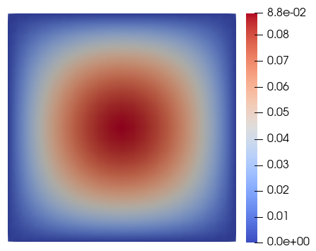
(a)

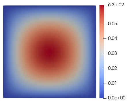
(b)

Figure 1: Numerical solutions at $T=1$; (a) Displacement $|u_{h}|$, (b) Pressure $p$.

Figure 2 shows the $L^{2}$ error of the pressure and the average number of iterations per time step for different mesh sizes. As the mesh is refined, the pressure converges with an order of 2. The average number of iterations is nearly mesh-independent, consistent with the theoretically established results for the quasi-static Biot model.

The average number of iterations per time step for different stabilization parameters with a fixed mesh size is displayed in Figure 3. In accordance with the quasi-static scheme, the stabilization parameter heavily influences the convergence rate. The fastest convergence is obtained for a smaller $L$ than the classical parameter.

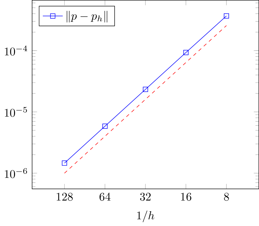
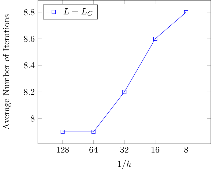
Figure 2: $L^{2}$ error of the pressure with a line (red) representing second-order convergence and the average number of iterations for different mesh sizes.

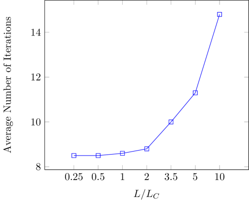
Figure 3: Average number of iterations per time step for different stabilization parameters with fixed mesh size $h=1/16$.

5 Conclusions

We considered a fully dynamic Biot model for flow and deformation in porous media. The model includes additional memory effects, containing a history-dependent permeability. We propose a fixed-stress type splitting scheme for efficiently solving this model. We performed a numerical experiment to study the convergence of the scheme. It is not clear under which situations the memory effects become important. This will be explored under more realistic parameter choices in further work.

- (1) Mikelić, A., Wheeler, M.F.: Convergence of iterative coupling for coupled flow and geomechanics. Comput. Geosci. 17, 455–461 (2013)
- (2) Both, J.W., Borregales, M., Nordbotten, J.M., Kumar, K., Radu, F.A.: Robust fixed stress splitting for Biot’s equations in heterogeneous media. Appl. Math. Lett. 68, 101–108 (2017)
- (3) Borregales, M., Radu, F.A., Kumar, K., Nordbotten, J.M.: Robust iterative schemes for non-linear poromechanics. Comput. Geosci. 22(4), 1021–1038 (2018)
- (4) Storvik, E., Both, J.W., Kumar, K., Nordbotten, J.M., Radu, F.A.: On the optimization of the fixed‐stress splitting for Biot’s equations. Int J Numer Methods Eng. 120(2), 179–194 (2019)
- (5) Mikelić, A., Wheeler, M.F.: Theory of the dynamic Biot-Allard equations and their link to the quasi-static Biot system. J. Math. Phys. 53(12), 123702 (2012)
- (6) Showalter, R.E.: Diffusion in Poro-Elastic Media. J. Math. Anal. 251(1), 310–340 (2000)
- (7) Bause, M., Anselmann, M., Köcher, U., Radu, F.A.: Convergence of a continuous Galerkin method for hyperbolic-parabolic systems, arXiv preprint arXiv:2201.12014 (2022)
- (8) Kim, J., Tchelepi, H.A., Juanes, R.: Stability, Accuracy, and Efficiency of Sequential Methods for Coupled Flow and Geomechanics. SPE Journal. 16(02), 249–262 (2011)
- (9) Bause, M., Both, J.W., Radu, F.A.: Iterative Coupling for Fully Dynamic Poroelasticity. In: Numerical Mathematics and Advanced Applications ENUMATH 2019. pp. 115–123.
- (10) Both, J.W., Kumar, K., Nordbotten, J.M., Radu, F.A.: The gradient flow structures of thermo-poro-visco-elastic processes in porous media, arXiv preprint arXiv:1907.03134 (2019)
- (11) Kraus, J., Kumar, K., Lymbery, M., Radu, F.A.: A fixed-stress type splitting method for nonlinear poroelasticity, arXiv preprint arXiv:2312.17698 (2023)
- (12) Bastian, P., et al: The Dune framework: Basic concepts and recent developments. Comput. Math. Appl. 81, 75–112 (2021)