Cost optimisation of individual-based institutional reward incentives for promoting cooperation in finite populations

Abstract

In this paper, we study the problem of cost optimisation of individual-based institutional incentives (reward, punishment, and hybrid) for guaranteeing a certain minimal level of cooperative behaviour in a well-mixed, finite population. In this scheme, the individuals in the population interact via cooperation dilemmas (Donation Game or Public Goods Game) in which institutional reward is carried out only if cooperation is not abundant enough (i.e., their number is below a threshold $1\leq t\leq N-1$, where $N$ is the population size); and similarly, institutional punishment is carried out only when defection is too abundant. We study analytically the cases $t=1$ for the reward incentive, showing that the cost function is always non-decreasing. We also derive the neutral drift and strong selection limits when the intensity of selection tends to zero and infinity, respectively. We also numerically investigate the problem for other values of $t$.

1 Introduction

Cooperation refers to an act of paying a cost in order to convey a benefit to someone else. It is one of the cornerstones of human civilisation and one of the reasons for our unprecedented success as a species [1]. Organisations are constantly faced with the problem of allocating resources in a budget-effective way. This issue becomes particularly essential for institutions like local governments and the United Nations, where the optimisation of resources is crucial in facilitating cooperative endeavors. Given the paramount importance of cooperation, these organisations are tasked with strategically managing the costs associated with incentivising collective efforts [18, 30].

A well-established theoretical framework for analysing the promotion of cooperation is Evolutionary Game Theory (EGT) [25], which has been used in both deterministic and stochastic settings. Using this framework, several mechanisms for promoting the evolution of cooperation have been studied including kin selection, direct reciprocity, indirect reciprocity, network reciprocity, group selection and different forms of incentives [16, 25, 19, 20, 30].

The current work focuses on institutional incentives [23, 26, 32, 6, 3, 27, 30, 8, 7, 27, 14], which is a plan of action involving the use of reward (i.e.,, increasing the payoff of cooperators), punishment (i.e.,, decreasing the payoff of defectors), or a combination of the two by an external decision-maker. More precisely, we study how the aforementioned institutional incentives can be used in a cost-efficient way for maximising the levels of cooperative behaviour in a population of self-regarding individuals. In the literature, although there is a significant amount of works using agent-based numerical simulations, there are a few papers that employ a rigorous analysis of the problem at hand [32, 10, 6, 5, 33, 34]. The works that do use analysis employ two complementary approaches, either in a continuous setting where the evolutionary processes are modelled as a continuous dynamical system (for instance, using the replicator dynamics) [32, 33, 34] or in a discrete setting, in which the population dynamics are modelled as a Markov chain [10, 6, 5]. We review in more detail both approaches in the next paragraphs since they are most relevant to the present work.

In the discrete setting, the evolutionary process is often described by a Markov chain with an update rule (for instance, in the absence of mutation, it is an imitation process with the Fermi strategy update rule). For well-mixed finite populations and general two-player two-strategy games, the problem of promoting the evolution of cooperative behaviour with a minimum cost is formulated and numerically studied in [10]. In this paper, the decision-maker may use a full-invest scheme, in which, in each generation, all cooperators are rewarded (or all defectors are punished) or an individual-based scheme, in which only cooperators (defectors) are rewarded (punished, respectively) only if cooperation is not frequent enough. In both cases, the expected total cost of interference is a finite sum, over the state space of the Markov chain, of per generation costs. In [6], the authors then analyse the cost function for a full-invest scheme in which individuals interact via public goods games or donation games. They prove that the cost function exhibits a phase transition when the intensity of selection varies and exactly calculate the optimal cost of the incentive for any given intensity of selection. In a more recent paper [5], similar results are obtained in the case of hybrid (mixed) reward and punishment incentives.

In the continuous setting, the evolutionary process is modelled by the replicator dynamics, which is a set of differential equations describing the evolution of the behavioural frequencies. For infinitely large, well-mixed populations, the problem of providing a minimum cost that guarantees a sufficient level of cooperation is formulated as an optimal control problem in [32]. By using the approach of the Hamilton-Jacobi-Bellman equation, the authors theoretically obtain the optimal reward (positive) or punishment (negative) incentive strategies with the minimal cumulative cost, respectively. Similar results for structured population are obtained in [34] (for either reward or punish incentive separately) and in [31] (for combined incentives), using pair approximate methods. In these papers, the decision-maker implements incentives centrally within the whole population. In [33], the authors consider the same problem but using decentralised incentives, that is, in each game group, a local incentive-providing institution implements local punishment or reward incentives on group members. We also refer the reader to [35] for a recent survey on this optimal control approach.

Overview of contribution of this paper.

Following the discrete approach in [10, 6, 5], in this work, we rigorously study the problem of cost optimisation of institutional reward or/and punishment for maximising the levels of cooperative behaviour (or guaranteeing at least a certain level of cooperation) for well-mixed, finite populations. We focus on individual-based schemes, in which, in each generation, only when the number of cooperators/defectors is below a certain threshold $t$ (with $1\leq t<N-1$, where $N$ is the population size), are they rewarded (punished, respectively) (the case of the full-invest scheme $t=N-1$ has been studied in [6, 5]).

Analysing this problem for an arbitrary value of $t$ would be very challenging due to the number of parameters involved such as the number of individuals in the population, the strength of selection, the game-specific quantities, as well as the efficiency ratios of providing the corresponding incentive. In particular, the Markov chain based evolutionary process is of order equal to the population size, which is large but finite. The calculation of the entries of the corresponding fundamental matrix, which appear in the cost function, is intricate, both analytically and computationally.

Our present work provides a rigorous analysis of this problem in the case of reward for $t=1$. The main analytical results of the paper can be summarised as follows.

1. We show that the cost function is always non-decreasing regardless of the values of other parameters.

2. We obtain the asymptotic behaviour of the cost function in the limits of neutral drift and strong selection when the intensity of selection goes to zero or infinity, respectively.

We also numerically investigate the cost function and its behaviour for other values of $t$.

The rest of the paper is organised as follows. In Section 2, we present the model and methods. Our main results are Theorem 2 on the monotonicity of the reward $t=1$ cost function and Propositions 1, 2 on the asymptotic behaviour (neutral drift, strong selection limits) of the reward $t=1$ cost function. In Section 5, we provide a numerical analysis of reward, punishment, and hybrid cost functions, highlighting their monotonicity as well as the behaviour of their derivatives. Summary and further discussions are provided in Section 6. Finally, Section 7 contains the derivative of the reward cost function, detailed calculations for obtaining the reward $t=2$ cost function, and small population computations.

2 Model and methods

In this section, we present the model and methods of the paper. We first introduce the class of games, namely cooperation dilemmas, that we are interested in throughout this work.

2.1 Evolutionary processes

We consider an evolutionary process of a well-mixed, finite population of $N$ interacting individuals (players). We adopt the finite population dynamics modelling as an absorbing Markov chain of $(N+1)$ states, $\{S_{0},...,S_{N}\}$, where $S_{j}$ represents a population with $j$ C players (and $N-j$ defectors) (the sates $S_{0}$ and $S_{N}$ are absorbing). We employ the Fermi strategy update rule [29] stating that a player $X$ with fitness $f_{X}$ adopts the strategy of another player $Y$ with fitness $f_{Y}$ with a probability given by $P_{X,Y}=\left(1+e^{-\beta(f_{Y}-f_{X})}\right)^{-1}$, where $\beta$ represents the intensity of selection.

2.2 Cooperation dilemmas

Individuals engage with one another using one of the following one-shot (i.e., non-repeated) cooperation dilemmas: the Donation Game (DG) or its multi-player version, the Public Goods Game (PGG). Strategy wise, each player can choose to either cooperate (C) or defect (D).

Let $\Pi_{C}(j)$ be the average payoff of a C player (cooperator) and $\Pi_{D}(j)$ that of a D player (defector), in a population with $j$ $C$ players and $(N-j)$ $D$ players. As can be seen below, the difference in payoffs $\delta=\Pi_{C}(j)-\Pi_{D}(j)$ in both games does not depend on $j$. For the two cooperation dilemmas considered in this paper, namely the Donation Games and the Public Goods Games, it is always the case that $\delta<0$. This does not cover some weak social dilemmas such as the snowdrift game, where $\delta>0$ for some $j$, the general prisoners’ dilemma, and the collective risk game [27], where $\delta$ depends on $j$.

Donation Game (DG)

The Donation Game is a form of Prisoners’ Dilemma in which cooperation corresponds to offering the other player a benefit $B$ at a personal cost $c$, satisfying that $B>c$. Defection means offering nothing. The payoff matrix of DG (for the row player) is given as follows

$$\bordermatrix{\leavevmode\nobreak\ &C&D\cr C&B-c&-c\cr D&B&0\cr}.$$

Denoting $\pi_{X,Y}$ the payoff of a strategist $X$ when playing with a strategist $Y$ from the payoff matrix above, we obtain

$$\begin{split}\Pi_{C}(j)&=\frac{(j-1)\pi_{C,C}+(N-j)\pi_{C,D}}{N-1}=\frac{(j-1)(B-c)+(N-j)(-c)}{N-1},\\ \Pi_{D}(j)&=\frac{j\pi_{D,C}+(N-j-1)\pi_{D,D}}{N-1}=\frac{jB}{N-1}.\end{split}$$

Thus,

$$\delta=\Pi_{C}(j)-\Pi_{D}(j)=-\Big{(}c+\frac{B}{N-1}\Big{)}.$$

Public Goods Game (PGG)

In a Public Goods Game, players interact in a group of size $n$, where they decide to cooperate, contributing an amount $c>0$ to a common pool, or to defect, contributing nothing to the pool. The total contribution in a group is multiplied by a factor $r$, where $1<r<n$ (for the PGG to be a social dilemma), which is then shared equally among all members of the group, regardless of their strategy. Intuitively, contributing nothing offers one a higher amount of money after redistribution.

The average payoffs, $\Pi_{C}(j)$ and $\Pi_{D}(j)$, are calculated based on the assumption that the groups engaging in a public goods game are given by multivariate hypergeometric sampling. Thereby, for transitions between two pure states, this reduces to sampling, without replacement, from a hypergeometric distribution. More precisely, we obtain [11]

$$\begin{split}\Pi_{C}(j)&=\sum^{n-1}_{i=0}\frac{\dbinom{j-1}{i}\dbinom{N-j}{n-1-i}}{\dbinom{N-1}{n-1}}\ \left(\frac{(i+1)rc}{n}-c\right)=\frac{rc}{n}\left(1+(j-1)\frac{n-1}{N-1}\right)-c,\\ \Pi_{D}(j)&=\sum^{n-1}_{i=0}\frac{\dbinom{j}{i}\dbinom{N-1-j}{n-1-i}}{\dbinom{N-1}{n-1}}\ \frac{jrc}{n}=\frac{rc(n-1)}{n(N-1)}j.\end{split}$$

Thus,

$$\delta=\Pi_{C}(j)-\Pi_{D}(j)=-c\left(1-\frac{r(N-n)}{n(N-1)}\right).$$

2.3 Cost of institutional incentives

To reward a cooperator (or to punish a defector), the institution has to pay an amount $\theta/a$ (or $\theta/b$ respectively) so that the cooperator’s (defector’s) payoff increases (decreases) by $\theta$, where $a,b>0$ are constants representing the efficiency ratios of providing this type of incentive.

In an institutional enforcement setting, we assume that the institution has full information about the population composition or statistics at the time of decision-making. That is, given the well-mixed population setting, we assume that the number $j$ of cooperators in the population is known. While reward and punishment and their usefulness as institutional incentives have been previously studied, including in [6, 5] which are most relevant to this work, the approach in the aforementioned papers is a ‘full-invest’ one, i.e., in each state of the evolutionary process, all cooperators (defectors) are rewarded (punished).

In the present paper, we consider investment schemes that reward (or/and punish) $t$ $C$ players ($N-t$ $D$ players) whenever the number of cooperators in the population does not exceed a given threshold $t$ for $1\leq t\leq N-1$. The argument for this type of approach and its applicability in real life is as follows. First, if cooperation is sufficiently frequent, the cooperators might survive by themselves without further need of costly incentives. Second, if the institution spreads their incentive budget for too many individuals, then the impact on each individual might not be enough to alter the global dynamics.

Hence, we have, for $1\leq j\leq t$, the cost per generation for the incentive providing institution is

$$\theta_{j}=\begin{cases}\frac{j}{a}\theta,\quad\text{reward incentive},\\ \frac{N-j}{b}\theta,\quad\text{punishment incentive},\\ \min\Big{(}\frac{j}{a},\frac{N-j}{b}\Big{)}\theta,\quad\text{mixed incentive},\end{cases}$$ (1)

while $\theta_{j}=0$ for $t<j\leq N-1$.

Next, to derive the total expected cost of inference over all generations, we assume that the population is equally likely to start in the homogeneous state $S_{0}$ as well as in the homogeneous state $S_{N}$. Let $(n_{ik})_{i,k=1}^{N-1}$ be the entries of the fundamental matrix of the absorbing Markov chain of the evolutionary process. The entries gives the expected number of times the population is in the state $S_{j}$ if it is started in the transient state $S_{i}$ [13]. Under the above assumption, a mutant can randomly equally occur either at $S_{0}$ or $S_{N}$, the expected number of visits at state $S_{j}$ ($1\leq j\leq N-1$) is thus $\frac{1}{2}(n_{1j}+n_{N-1,j})$. Therefore the expected cost of inference over all generations is given by

$$E(\theta)=\frac{1}{2}\sum_{j=1}^{N-1}(n_{1j}+n_{N-1,j})\theta_{j}=\frac{1}{2}\sum_{j=1}^{t}(n_{1j}+n_{N-1,j})\theta_{j},$$ (2)

where the second equality follows from the individual-based incentive (1).

Remark.

We comment on our assumption that the population is equally likely to start in the homogeneous state. This assumption is reasonable when the mutation is negligible and is often made in many works based on agent-based simulations [2, 4, 28, 9, 24] (in these works, simulations end whenever the population fixates in a homogeneous state). Our model therefore encapsulates the intermediate-run dynamics, an approximation that is valid if the time-scale is long enough for one type to reach fixation, but too short for the next mutant to appear. It might thus be more practically useful for the optimisation of the institutional budget for providing incentives on an intermediate timescale.

In the most general case when mutation is frequent, the above assumption might not be suitable. For example, if cooperators are very likely to fixate in a population of defectors, but defectors are unlikely to fixate in a population of cooperators, mutants are on average more likely to appear in the homogeneous cooperative population (that is in $S_{N}$). Similarly, if defectors are very likely to fixate in a population of cooperators, but cooperators are unlikely to fixate in a population of defectors, mutants are on average more likely to appear in $S_{0}$ rather than $S_{N}$. In general, in the long-run, the population will start at $i=0$ ($i=N$, respectively) with probability equal to the frequency of D (C) computed at the equilibrium, $f_{D}=1/(r+1)$ ($f_{C}=r/(r+1)$, respectively), where $r=e^{\beta(N-1)(\delta+\theta)}$. Thus, generally, the expected number of visits at state $S_{i}$ will be $f_{D}n_{1i}+f_{C}n_{N-1,i}$. We will study the general setting in future work.

2.3.1 Cooperation frequency and optimal incentives

Next we construct the problem of cost optimisation of individual-based institutional incentives (reward, punishment, and hybrid) for maximising the level (or guaranteeing at least a certain level) of cooperative behaviour.

Since the population consists of only two strategies, the fixation probabilities of a C (D) player in a homogeneous population of D (C) players when the interference scheme is carried out are, respectively, [15]

$$\begin{split}\rho_{D,C}&=\left(1+\sum_{i=1}^{N-1}\prod_{k=1}^{i}\frac{1+e^{\beta(\Pi_{C}(k)-\Pi_{D}(k)+\delta(k)\theta)}}{1+e^{-\beta(\Pi_{C}(k)-\Pi_{D}(k)+\delta(k)\theta)}}\right)^{-1},\\ \rho_{C,D}&=\left(1+\sum_{i=1}^{N-1}\prod_{k=1}^{i}\frac{1+e^{\beta(\Pi_{D}(k)-\Pi_{C}(k)-\delta(k)\theta)}}{1+e^{-\beta(\Pi_{D}(k)-\Pi_{C}(k)-\delta(k)\theta)}}\right)^{-1}.\end{split}$$

where $\delta(k)=1$ if $k\leq t$ and $\delta(k)=0$ otherwise.

Computing the stationary distribution using these fixation probabilities, we obtain the frequency of cooperation

$$\frac{\rho_{D,C}}{\rho_{D,C}+\rho_{C,D}}.$$

Hence, this frequency of cooperation can be maximised by maximising

$$\max_{\theta}\left(\rho_{D,C}/\rho_{C,D}\right).$$ (3)

The fraction in Equation (3) can be simplified as follows [16]

$$\frac{\rho_{D,C}}{\rho_{C,D}} = \prod_{k=1}^{N-1}\frac{u_{i,i-1}}{u_{i,i+1}}=\prod_{k=1}^{N-1}\frac{1+e^{\beta[\Pi_{C}(k)-\Pi_{D}(k)+\delta(k)\theta]}}{1+e^{-\beta[\Pi_{C}(k)-\Pi_{D}(k)+\delta(k)\theta]}}$$

$$= e^{\beta\sum_{k=1}^{N-1}\left(\Pi_{C}(k)-\Pi_{D}(k)+\delta(k)\theta\right)}$$

$$= e^{\beta[(N-1)\delta+t\theta]}.$$

In the above transformation, $u_{i,i-1}$ and $u_{i,i-1}$ are the probabilities to decrease or increase the number of C players (i.e., $i$) by one in each time step, respectively.

Under neutral selection (i.e., when $\beta=0$), there is no need to use incentives as no player is likely to copy another player and any changes in strategy that happen are due to noise as opposed to incentives. Thus, we only consider $\beta>0$. The goal is to ensure at least an $\omega\in[0,1]$ fraction of cooperation, i.e., $\frac{\rho_{D,C}}{\rho_{D,C}+\rho_{C,D}}\geq\omega$. Thus, it follows from the equation above that

$$\theta\geq\theta_{0}(\omega)=\frac{1}{t}\left(\frac{1}{\beta}\log\left(\frac{\omega}{1-\omega}\right)-(N-1)\delta\right).$$ (4)

It is guaranteed that if $\theta\geq\theta_{0}(\omega)$, at least an $\omega$ fraction of cooperation is expected in the long run. This condition implies that the lower bound of $\theta$ monotonically depends on $\beta$. Namely, when $\omega\geq 0.5$, it increases with $\beta$ and when $\omega<0.5$, it decreases with $\beta$.

Bringing all together, we obtain the following mathematical constrained minimisation problem of individual-based institutional incentives (reward, punishment, and hybrid) guaranteeing at least a certain level of cooperative behaviour:

$$\min_{\theta\geq\theta_{0}}E(\theta),$$ (5)

where $E(\theta)$ can either be the reward ($E_{r}(\theta)$), punishment ($E_{p}(\theta)$), or hybrid cost function ( $E_{mix}(\theta)$).

The main aim of this paper is study the above optimisation problem. We focus on the reward incentive, in which the decision-maker rewards $j$ cooperators whenever $j\leq t$, as in (1) (thus, we will set $a=1$ in (1) throughout the paper since it does not affect our optimisation problem). In principle, the punishment and mixed incentives are similar, and we only provide numerical investigations for these schemes.

For $t=1$, we analytically show that $E_{r}(\theta)$ is non-decreasing as a function of $\theta$ for all values of other parameters. We also establish the neutral and strong selection limits of $E_{r}(\theta)$, that is

$$\lim_{\beta\rightarrow 0}E_{r}(\theta)\quad\text{and}\quad\lim_{\beta\rightarrow\infty}E_{r}(\theta).$$

For other values of $t$, we numerically investigate the properties of $E_{r}(\theta)$.

3 Reward incentive

We first calculate the cost function, $E_{r}(\theta)$, more explicitly. To this end, we compute the expected number of times the population contains $j$ C players, $1\leq j\leq N-1$. Let $U=\{u_{ij}\}_{i,j=1}^{N-1}$ denote the transition matrix between the $N-1$ transient states, $\{S_{1},...,S_{N-1}\}$. According to the Fermi update rule, the transition matrix is given as follows:

$$\begin{split}u_{i,i\pm k}&=0\qquad\text{ for all }k\geq 2,\\ u_{i,i\pm 1}&=\frac{N-i}{N}\frac{i}{N}\left(1+e^{\mp\beta[\Pi_{C}(i)-\Pi_{D}(i)+\theta_{i}/i]}\right)^{-1},\\ u_{i,i}&=1-u_{i,i+1}-u_{i,i-1}.\end{split}$$ (6)

For simplicity, we normalise $a=1$, and obtain (recalling that $\Pi_{C}(i)-\Pi_{D}(i)=\delta$ for all $1\leq i\leq N-1$, and $\theta_{i}/i=\frac{\theta}{a}=\theta$ for $1\leq i\leq t$ and zero otherwise):

$$u_{i,i\pm k}=0\quad\text{for}\quad k\geq 2,$$

$$u_{i,i+1}=\begin{cases}\frac{(N-i)i}{N^{2}}\Big{(}1+e^{-\beta(\delta+\theta)}\Big{)}\quad\text{for}\quad 1\leq i\leq t,\\ \frac{(N-i)i}{N^{2}}\Big{(}1+e^{-\beta\delta}\Big{)}\quad\text{for}\quad t<i\leq N-1,\\ \end{cases}$$

$$u_{i,i-1}=\begin{cases}\frac{(N-i)i}{N^{2}}\Big{(}1+e^{\beta(\delta+\theta)}\Big{)}\quad\text{for}\quad 1\leq i\leq t,\\ \frac{(N-i)i}{N^{2}}\Big{(}1+e^{\beta\delta}\Big{)}\quad\text{for}\quad t<i\leq N-1,\\ \end{cases}$$

$$u_{i,i} =1-u_{i,i+1}-u_{i,i-1}.$$

Next, we need to calculate the entries $n_{ik}$ of the fundamental matrix $\mathcal{N}=(n_{ik})_{i,k=1}^{N-1}=(I-U)^{-1}$. By using $\frac{1}{1+m}+\frac{1}{1+\frac{1}{m}}=1$ for $m=e^{\beta[\Pi_{C}(i)-\Pi_{D}(i)+\theta_{i}/i]}$, we get $u_{i,i+1}+u_{i,i-1}=\frac{N-i}{N}\frac{i}{N}$. Then, by letting $V=(I-U)$, we obtain:

$$\begin{split}v_{i,i\pm k}&=0\qquad\text{ for all }k\geq 2,\\ v_{i,i\pm 1}&=-\frac{N-i}{N}\frac{i}{N}\left(1+e^{\mp\beta[\Pi_{C}(i)-\Pi_{D}(i)+\theta_{i}/i]}\right)^{-1},\\ v_{i,i}&=u_{i,i+1}+u_{i,i-1}=\frac{N-i}{N}\frac{i}{N}.\end{split}$$ (7)

We can further write $V=W\mathrm{diag}\Big{\{}\frac{N-1}{N}\frac{1}{N},\ldots,\frac{N-i}{N}\frac{i}{N},\ldots,\frac{1}{N}\frac{N-1}{N}\Big{\}}$, where

$$W=\begin{pmatrix}1&-a&&&&&\\ -c&1&-a&&&&&\\ &\ddots&\ddots&\ddots&&&\\ &&-c&1&-a&&&\\ &&&-d&1&-b&&&\\ &&&&\ddots&\ddots&\ddots&\\ &&&&&-d&1&-b\\ &&&&&&-d&1\end{pmatrix},$$ (8)

with $a:=(1+e^{-\beta(\delta+\theta)})^{-1},\quad b:=(1+e^{-\beta\delta})^{-1},\quad c:=(1+e^{\beta(\delta+\theta)})^{-1},\quad d:=(1+e^{\beta\delta})^{-1}$.

This implies that $\mathcal{N}=V^{-1}=\mathrm{diag}\Big{\{}\frac{N^{2}}{N-1},\frac{N^{2}}{2(N-2)},\ldots,\frac{N^{2}}{N-1}\Big{\}}W^{-1}$, and so, the fundamental matrix is $\mathcal{N}=\mathrm{diag}\Big{\{}\frac{N^{2}}{N-1},\frac{N^{2}}{2(N-2)},\ldots,\frac{N^{2}}{N-1}\Big{\}}(n_{ik})_{i,k=1}^{N-1}=W^{-1}$.

Therefore, the expected total cost of interference for reward is

$$E_{r}(\theta) =\frac{1}{2}\sum_{j=1}^{N-1}(n_{1j}+n_{N-1,j})\theta_{j}$$

$$=\frac{1}{2}\sum_{j=1}^{t}(n_{1j}+n_{N-1,j})\theta_{j}$$

$$=\frac{N^{2}\theta}{2}\sum_{j=1}^{t}\frac{(W^{-1})_{1j}+(W^{-1})_{N-1,j}}{N-j},$$ (9)

where $\theta_{j}=\theta j$ follows from Equation 2 normalised with $a=1$.

The advantage of expressing the cost function in terms of the entries of the matrix $W$ is that this matrix is tri-diagonal. The inverse of a tri-diagonal matrix can be theoretically computed using recursive formulae, see e.g., [12]. In general, these formulae are still very hard to analytically explore. However, in the special extreme cases $t=1$ and $t=N-1$, we can explicitly obtain the entries of the inverse matrix $W^{-1}$. Therefore, we obtain analytically the explicit formula for the cost function. The case $t=N-1$ has already been studied in [6, 5]. Thus in this paper, we study the case $t=1$, which will be discussed in detail next.

3.1 Institutional Reward with $t=1$

In this section, we introduce the analytical results related to the case of institutional reward with $t=1$, when the institution provides reward only when there is a single cooperator in the population. We present the cost function for this particular case together with information on its monotonicity, as well as the limits for the neutral drift and strong selection.

The reward cost function for the threshold value $t=1$ is

$$E_{r}(\theta)=\frac{N^{2}\theta}{2}\frac{(W^{-1})_{1,1}+(W^{-1})_{N-1,1}}{N-1},$$ (10)

obtained by substituting $t=1$ in (3). Next we compute explicitly the entries $(W^{-1})_{1,1}$ and $(W^{-1})_{N-1,1}$. Noting that for $t=1$, the matrix $W$ is a special case of a tri-diagonal matrix of the form

$$A=\left[\begin{array}[]{ccccccc}b_{1}&c_{1}&&&&&\\ a_{2}&b_{2}&c_{2}&&&&\\ &\ddots&\ddots&\ddots&&&\\ &&a_{j}&b_{j}&c_{j}&&\\ &&&\ddots&\ddots&\ddots&\\ &&&&a_{n-1}&b_{n-1}&c_{n-1}\\ &&&&&a_{n}&b_{n}\end{array}\right].$$

We recall the following result from [12] that provides analytical formulae for the entries of the inverse matrix $A^{-1}$. We will then apply this result to calculate $(W^{-1})_{1,1}$ and $(W^{-1})_{N-1,1}$.

Theorem 1.

([12]) Define the second-order linear recurrences

$$z_{i}=b_{i}z_{i-1}-a_{i}c_{i-1}z_{i-2}\quad i=2,3,\ldots,n$$

where $z_{0}=1,z_{1}=b_{1}$, and

$$y_{j}=b_{j}y_{j+1}-a_{j+1}c_{j}y_{j+2}\quad j=n-1,n-2,\ldots,1$$

where $y_{n+1}=1,y_{n}=b_{n}$. The inverse matrix $A^{-1}=\left\{\phi_{i,j}\right\}(1\leqslant i,j\leqslant n)$ can be expressed as

$$\phi_{j,j}=\frac{1}{b_{j}-a_{j}c_{j-1}\frac{z_{j-2}}{z_{j-1}}-a_{j+1}c_{j}\frac{y_{j+2}}{y_{j+1}}}$$

where $j=1,2,\ldots,n,a_{1}=0,c_{n}=0$ and

$$\phi_{i,j}=\begin{cases}-c_{i}\frac{z_{i-1}}{z_{i}}\phi_{i+1,j}&i<j\\ -a_{i}\frac{y_{i+1}}{y_{i}}\phi_{i-1,j}&i>j.\end{cases}$$

Corollary 1.

([12])

The inverse matrix $A^{-1}=\left\{\phi_{i,j}\right\}$ can be expressed as

$$\phi_{j,j}=\frac{1}{b_{j}-a_{j}c_{j-1}\frac{z_{j-2}}{z_{j-1}}-a_{j+1}c_{j}\frac{y_{j+2}}{y_{j+1}}},$$

where $j=1,2,\ldots,n,\ a_{1}=0$, $c_{n}=0$ and

$$\phi_{i,j}=\begin{cases}(-1)^{j-i}\left(\prod_{k=1}^{j-i}c_{j-k}\right)\frac{z_{i-1}}{z_{j-1}}\phi_{j,j}&i<j\\ (-1)^{i-j}\left(\prod_{k=1}^{i-j}a_{j+k}\right)\frac{y_{i+1}}{y_{j+1}}\phi_{j,j}&i>j.\end{cases}$$

We use the above results to derive the following lemma which provides explicit formula for the reward cost function for $t=1$.

Lemma 1.

For $t=1$, we have

$$E_{r}(\theta)=\frac{N^{2}\theta}{2(N-1)}\Big{(}1+d^{N-2}\frac{1}{y_{2}}\Big{)}\frac{1}{1-ad\frac{y_{3}}{y_{2}}},$$ (11)

where $y_{2}$ and $y_{3}$ are found from the following backward recursive formula:

$$y_{N}=1,\quad y_{N-1}=1,\quad\text{and}\quad y_{N-i}=y_{N-i+1}-(bd)y_{N-i+2},\quad\text{for}\quad i=1,\ldots,N-2.$$ (12)

Proof.

We compute the two entries $W^{-1}_{1,1}$ and $W^{-1}_{N-1,1}$ appearing in (10) using Theorem 1. We recall that

$$W=\begin{pmatrix}1&-a&&&&&\\ -c&1&-a&&&&&\\ &\ddots&\ddots&\ddots&&&\\ &&-c&1&-a&&&\\ &&&-d&1&-b&&&\\ &&&&\ddots&\ddots&\ddots&\\ &&&&&-d&1&-b\\ &&&&&&-d&1\end{pmatrix},$$

with

$$a:=(1+e^{-\beta(\delta+\theta)})^{-1},\quad b:=(1+e^{-\beta\delta})^{-1},\quad c:=(1+e^{\beta(\delta+\theta)})^{-1},\quad d:=(1+e^{\beta\delta})^{-1}.$$

In particular, for $t=1$, we obtain

$$W=\begin{pmatrix}1&-a&&&&&\\ -d&1&-b&&&&&\\ &\ddots&\ddots&\ddots&&&\\ &&-d&1&-b&&&\\ &&&-d&1&-b&&&\\ &&&&\ddots&\ddots&\ddots&\\ &&&&&-d&1&-b\\ &&&&&&-d&1\end{pmatrix}$$

We apply Theorem 1, the diagonal element case, and Corollary 1, the $i>j$ case, to obtain

$$W^{-1}_{1,1} =\frac{1}{1-ad\frac{y_{3}}{y_{2}}},$$

$$(W^{-1})_{N-1,1} =(-1)^{N-2}\Big{(}\prod\limits_{k=1}^{N-2}a_{k+1}\Big{)}\frac{y_{N}}{y_{2}}\phi_{1,1}$$

$$=(-1)^{N-2}\Bigg{(}\prod\limits_{k=1}^{N-2}a_{k+1}\Bigg{)}\frac{1}{y_{2}}\frac{1}{1-ad\frac{y_{3}}{y_{2}}}$$

$$=d^{N-2}\frac{1}{y_{2}}\frac{1}{1-ad\frac{y_{3}}{y_{2}}}.$$

In the above formulae, $y_{2}$ and $y_{3}$ are found from the backward recursive formula (12). Thus, by summing up the above expressions, we obtain

$$(W^{-1})_{1,1}+(W^{-1})_{N-1,1} =\frac{1}{1-ad\frac{y_{3}}{y_{2}}}+d^{N-2}\frac{1}{y_{2}}\frac{1}{1-ad\frac{y_{3}}{y_{2}}}$$

$$=\Big{(}1+d^{N-2}\frac{1}{y_{2}}\Big{)}\frac{1}{1-ad\frac{y_{3}}{y_{2}}}.$$

Substituting the above into (10), we obtain

$$E_{r}(\theta) =\frac{N^{2}\theta}{2(N-1)}\Big{(}1+d^{N-2}\frac{1}{y_{2}}\Big{)}\frac{1}{1-ad\frac{y_{3}}{y_{2}}},$$

which completes the proof of this lemma. ∎

We now calculate explicitly $y_{2}$ and $y_{3}$ using the backward recursive formula (12):

$$\left\{\begin{array}[]{l}y_{N-1}=1,y_{N}=1\\ y_{j}=y_{j+1}-(bd)y_{j+2}\hskip 2.84526pt\forall\hskip 2.84526ptj=N-2,\ldots,2.\\ \end{array}\right.$$

For convenience, we transform the above backward recursive relation to a forward one. By applying a change of variable $\hat{y}_{j}=y_{N-j}$, we get

$$\left\{\begin{array}[]{l}\hat{y}_{0}=1,\quad\hat{y}_{1}=1.\\ \hat{y}_{j}=\hat{y}_{j-1}-(bd)\hat{y}_{j-2}\quad\forall j=2,\ldots,N.\end{array}\right.$$

By induction, it follows that $\hat{y}_{j}$ can be written in the form

$$\hat{y}_{j}=\sum_{k=0}^{j}m_{k}(bd)^{k}.$$

We observe that the coefficients of the recurrence relation follow the pattern in the table below.

		$(bd)^{0}$	$(bd)^{1}$	$(bd)^{2}$	$(bd)^{3}$	$(bd)^{4}$	$(bd)^{5}$
$\hat{y}_{0}$		1	0	0	0	0	0
$\hat{y}_{1}$		1	0	0	0	0	0
$\hat{y}_{2}$		1	-1	0	0	0	0
$\hat{y}_{3}$		1	-2	0	0	0	0
$\hat{y}_{4}$		1	-3	1	0	0	0
$\hat{y}_{5}$		1	-4	3	0	0	0
$\hat{y}_{6}$		1	-5	6	-1	0	0
$\hat{y}_{7}$		1	-6	10	-4	0	0
$\hat{y}_{8}$		1	-7	15	-10	1	0
$\hat{y}_{9}$		1	-8	21	-20	5	0

Table 1: Pattern for the coefficients in the expansion of $\hat{y}_{j}$, $j=0,1\,\ldots$,  in terms of the power of $(bd)$.

We observe that the entries of Table 1 are the binomial coefficients offset by a factor of $k$ for every column and are alternating in sign. This suggests that $\hat{y}_{j}=\sum\limits_{k=0}^{j}(-1)^{k}{j-k\choose k}(bd)^{k}$. In the lemma below, we prove this is indeed the case. We also obtain another expression for $\hat{y}_{j}$ using the general formula of a second order homogeneous recurrence relation.

Lemma 2 (Recurrence relation).

The following formulae hold for any $j\geq 0$

1. $\hat{y}_{j}=\sum\limits_{k=0}^{\lfloor\frac{j}{2}\rfloor}(-1)^{k}{j-k\choose k}(bd)^{k}$,

2. $\hat{y}_{j}=\frac{x_{1}x_{2}\left(x_{1}^{j-1}-x_{2}^{j-1}\right)-\left(x_{1}^{j}-x_{2}^{j}\right)}{x_{2}-x_{1}}$,

where

$$x_{1,2}=\frac{1\pm\sqrt{1-4bd}}{2}.$$

Proof.

We prove the first statement by induction on $j$. For $j=2$ we have $\hat{y}_{2}=\hat{y}_{1}-(bd)\hat{y}_{0}=1-bd$. We assume the statement holds for $j$ and need to prove it for $j+1$. Infact, we have

$$\hat{y}_{j+1} =\hat{y}_{j}-(bd)\hat{y}_{j-1}$$

$$=\sum_{k=0}^{\lfloor\frac{j}{2}\rfloor}(-1)^{k}{j-k\choose k}(bd)^{k}-(bd)\sum_{k=0}^{\lfloor\frac{j-1}{2}\rfloor}(-1)^{k}{j-1-k\choose k}(bd)^{k}$$

$$=\sum_{k=0}^{\lfloor\frac{j}{2}\rfloor}(-1)^{k}{j-k\choose k}(bd)^{k}-\Bigg{(}\sum_{k=0}^{\lfloor\frac{j-1}{2}\rfloor}(-1)^{k}{j-1-k\choose k}(bd)^{k+1}\Bigg{)}$$

$$=\sum_{k=0}^{\lfloor\frac{j}{2}\rfloor}(-1)^{k}{j-k\choose k}(bd)^{k}-\sum_{k=1}^{\lfloor\frac{j+1}{2}\rfloor}(-1)^{k-1}{j-k\choose k-1}(bd)^{k}$$

$$=1+\sum_{k=1}^{\lfloor\frac{j}{2}\rfloor}\Bigg{(}(-1)^{k}{j-k\choose k}-(-1)^{k-1}{j-k\choose k-1}\Bigg{)}(bd)^{k}-(-1)^{\lfloor\frac{j+1}{2}\rfloor-1}{j-\lfloor\frac{j+1}{2}\rfloor\choose\lfloor\frac{j+1}{2}\rfloor-1}(bd)^{\lfloor\frac{j+1}{2}\rfloor}$$

$$=1+\sum_{k=1}^{\lfloor\frac{j}{2}\rfloor}(-1)^{k}\Bigg{(}{j-k\choose k}+{j-k\choose k-1}\Bigg{)}(bd)^{k}+(-1)^{\lfloor\frac{j+1}{2}\rfloor}{j-\lfloor\frac{j+1}{2}\rfloor\choose\lfloor\frac{j+1}{2}\rfloor-1}(bd)^{\lfloor\frac{j+1}{2}\rfloor}$$ (13)

$$=1+\sum_{k=1}^{\lfloor\frac{j}{2}\rfloor}(-1)^{k}{j+1-k\choose k}(bd)^{k}+(-1)^{\lfloor\frac{j+1}{2}\rfloor}{j-\lfloor\frac{j+1}{2}\rfloor\choose\lfloor\frac{j+1}{2}\rfloor-1}(bd)^{\lfloor\frac{j+1}{2}\rfloor}$$

$$=\sum_{k=0}^{\lfloor\frac{j+1}{2}\rfloor}(-1)^{k}{j+1-k\choose k}(bd)^{k},$$

where to obtain (3.1), we used Pascal’s identity

$${j-k\choose k}+{j-k\choose k-1}={j+1-k\choose k}\quad\text{for}\quad 1\leq k\leq\lfloor\frac{j}{2}\rfloor$$

and

$${j+1-\lfloor\frac{j+1}{2}\rfloor\choose\lfloor\frac{j+1}{2}\rfloor}={j-\lfloor\frac{j+1}{2}\rfloor\choose\lfloor\frac{j+1}{2}\rfloor}+{j-\lfloor\frac{j+1}{2}\rfloor\choose\lfloor\frac{j+1}{2}\rfloor-1},$$

with ${j-\lfloor\frac{j+1}{2}\rfloor\choose\lfloor\frac{j+1}{2}\rfloor-1}=0$ as $\lfloor\frac{j+1}{2}\rfloor-1>j-\lfloor\frac{j+1}{2}\rfloor$.

Moreover, $\lfloor\frac{j-1}{2}\rfloor+1=n+1=\lfloor\frac{j+1}{2}\rfloor$ if $j=2n+1$ and $\lfloor\frac{j-1}{2}\rfloor+1=n=\lfloor\frac{j+1}{2}\rfloor$ if $j=2n$.

For the proof of the second statement, we note that $\hat{y}_{j}=\hat{y}_{j-1}-(bd)\hat{y}_{j-2}$ is a second order homogeneous recurrence relation and we solve it using the characteristic equation

$$x^{2}-x+bd=0.$$

Recall $b=\frac{1}{1+e^{-\beta\delta}}$ and $d=\frac{1}{1+e^{\beta\delta}}$, so

$$bd =\frac{1}{\left(1+e^{\beta\delta}\right)\left(1+e^{-\beta\delta}\right)}$$

$$=\frac{1}{2+e^{\beta\delta}+e^{-\beta\delta}}.$$

Since $e^{\beta\delta}+e^{-\beta\delta}\geq 2\sqrt{e^{\beta\delta}e^{-\beta\delta}}=2$, $bd<\frac{1}{4}$ $(\text{as }\beta,\delta\neq 0)$.
Therefore, the characteristic equation has two real solutions

$$x_{1,2}=\frac{1\pm\sqrt{1-4bd}}{2}.$$

Thus, we can express $\hat{y}_{i}$ using these roots as

$$\hat{y}_{j}=r_{1}x_{1}^{j}+r_{2}x_{2}^{j},$$

where the two constants are found from the initial data:

$$\hat{y}_{0}=r_{1}+r_{2}=1\quad\text{and}\quad\hat{y}_{1}=r_{1}x_{1}+r_{2}x_{2}=1.$$

Solving the above system for $r_{1},r_{2}$ results in

$$r_{1}=\frac{x_{2}-1}{x_{2}-x_{1}},\quad r_{2}=\frac{1-x_{1}}{x_{2}-x_{1}}.$$

Hence

$$\hat{y}_{j} =\frac{x_{2}-1}{x_{2}-x_{1}}x_{1}^{j}-\frac{x_{1}-1}{x_{2}-x_{1}}x_{2}^{j}$$

$$=\frac{x_{1}^{j}x_{2}-x_{1}x_{2}^{j}-\left(x_{1}^{j}-x_{2}^{j}\right)}{\left(x_{2}-x_{1}\right)}$$

$$=\frac{x_{1}x_{2}\left(x_{1}^{j-1}-x_{2}^{j-1}\right)-\left(x_{1}^{j}-x_{2}^{j}\right)}{x_{2}-x_{1}}.$$

This completes the proof of the Lemma. ∎

The following theorem, which is the main analytical result of the present paper, provides an explicit formula for the reward cost function $E_{r}(\theta)$ and shows that it is always non-decreasing for all parameter values.

Theorem 2 (Derivative and monotonicity of the cost function).

$E_{r}^{\prime}(\theta)$ is always increasing for all values of $N,\theta,\beta$, where

$$E_{r}^{\prime}(\theta)=\frac{N^{2}}{(2N-2)}\Big{(}y_{2}+d^{N-2}\Big{)}\Big{(}\frac{1}{y_{2}-ady_{3}}\Big{)}\Big{[}1+\frac{\theta dy_{3}\beta e^{-\beta(\delta+\theta)}a^{2}}{y_{2}-ady_{3}}\Big{]}.$$

As a consequence, the minimisation problem (5) has a unique solution

$$\min\limits_{\theta\geq\theta_{0}}E_{r}(\theta)=E_{r}(\theta_{0}).$$

Proof.

Recalling from Lemma 1 that

$$E_{r}(\theta)=\frac{N^{2}\theta}{2N-2}(y_{2}+d^{N-2})\Big{(}\frac{1}{y_{2}-ady_{3}}\Big{)}.$$

Next we will compute the derivative of $E_{r}(\theta)$ with respect to $\theta$.

Note that only $a$ depends on $\theta$

$$a=a(\theta)=(1+e^{-\beta(\theta+\delta)})^{-1},\quad a^{\prime}(\theta)=\frac{\beta e^{-\beta(\delta+\theta)}}{(1+e^{-\beta(\theta+\delta})^{2}}=\beta e^{-\beta(\delta+\theta)}a^{2},$$

while $b=(1+e^{-\beta\delta})^{-1}$ and $d=(1+e^{\beta\delta})^{-1}$ (and thus $y_{2}$ and $y_{3}$) do not depend on $\theta$. Let

$$C=C(\theta)=\frac{1}{y_{2}-ady_{3}}.$$

Then the derivative of $C$ with respect to $\theta$ is given by

$$C^{\prime}(\theta) =\frac{dy_{3}a^{\prime}(\theta)}{(y_{2}-ady_{3})^{2}}$$

$$=\frac{dy_{3}\beta e^{-\beta(\delta+\theta)}a^{2}}{(y_{2}-ady_{3})^{2}}$$

$$=\frac{dy_{3}\beta e^{-\beta(\delta+\theta)}a^{2}}{(y_{2}-ady_{3})}C(\theta)$$

$$=\frac{y_{3}\beta e^{-\beta\left(\delta+\theta\right)}}{\left(1+e^{-\beta\left(\delta+\theta\right)}\right)^{2}\left(y_{2}-\frac{y_{3}}{\left(1+e^{-\beta\left(\delta+\theta\right)}\right)\left(1+e^{\beta\delta}\right)}\right)^{2}\left(1+e^{\beta\delta}\right)}.$$

We calculate $E^{\prime}_{r}(\theta)$ via the product rule:

$$E_{r}^{\prime}(\theta) =\frac{N^{2}}{2N-2}(y_{2}+d^{N-2})\Big{[}C(\theta)+\theta C^{\prime}(\theta)\Big{]}$$

$$=\frac{N^{2}}{2N-2}(y_{2}+d^{N-2})\Big{[}1+\frac{\theta dy_{3}\beta e^{-\beta(\delta+\theta)}a^{2}}{y_{2}-ady_{3}}\Big{]}C(\theta)$$

$$=\frac{N^{2}}{(2N-2)}\Big{(}y_{2}+d^{N-2}\Big{)}\Big{(}\frac{1}{y_{2}-ady_{3}}\Big{)}\Big{[}1+\frac{\theta dy_{3}\beta e^{-\beta(\delta+\theta)}a^{2}}{y_{2}-ady_{3}}\Big{]}.$$

From the formula of $E_{r}(\theta)$ it follows that $y_{2}-ady_{3}>0$.
Next we will show that $y_{2}>0$ and $y_{3}>0$. Recalling that $y_{2}=\hat{y}_{N-1}$ and $y_{3}=\hat{y}_{N-2}$ where the sequence of numbers $(\hat{y})_{j}$ are given in Lemma 2. We will show that $\hat{y}_{j}>0$ for all $j\geq 0$.

In fact, according to the second statement of Lemma 2 we have

$$\hat{y}_{j} =\frac{x_{1}x_{2}\left(x_{1}^{j-1}-x_{2}^{j-1}\right)-\left(x_{1}^{j}-x_{2}^{j}\right)}{x_{2}-x_{1}}$$

$$=\frac{x_{1}x_{2}(x_{1}-x_{2})\sum\limits_{k=0}^{j-2}x_{1}^{k}x_{2}^{j-2-k}-(x_{1}-x_{2})\sum\limits_{k=0}^{j-1}x_{1}^{k}x_{2}^{j-1-k}}{x_{2}-x_{1}}$$

$$=\sum\limits_{k=0}^{j-1}x_{1}^{k}x_{2}^{j-1-k}-\sum\limits_{k=0}^{j-2}x_{1}^{k+1}x_{2}^{j-1-k}$$

$$=\sum\limits_{k=0}^{j-2}x_{1}^{k}x_{2}^{j-1-k}+x_{1}^{j-1}x_{2}^{0}-\sum\limits_{k=0}^{j-2}x_{1}^{k+1}x_{2}^{j-1-k}$$

$$=\sum\limits_{k=0}^{j-2}(x_{1}^{k}x_{2}^{j-1-k}-x_{1}^{k+1}x_{2}^{j-1-k})+x_{1}^{j-1}$$

$$=\sum\limits_{k=0}^{j-2}x_{1}^{k}x_{2}^{j-1-k}(1-x_{1})+x_{1}^{j-1}>0,$$

as $x_{1},x_{2}\in(0,1)$. Hence $y_{2},y_{3}>0$. Therefore, $E_{r}^{\prime}(\theta)>0$ for all $\theta>0$. ∎

3.2 Asymptotic limits

In this section, we study the neutral drift and strong selection limits of the reward cost function $E_{r}(\theta)$ (still with $t=1$) when the intensity of selection $\beta$ tends to $0$ and to +$\infty$, respectively.

Proposition 1.

(Neutral drift limit) It holds that

$$\lim\limits_{\beta\rightarrow 0}E_{r}(\theta)=\frac{N^{2}\theta}{N-1}\Bigg{(}P(N)+\frac{1}{2^{N-2}}\Bigg{)}\Big{(}\frac{2}{4P(N)-Q(N)}\Big{)},$$

where

$$P(N) =1+(-1)^{1}{N-2-1\choose 1}\Big{(}\frac{1}{4}\Big{)}^{1}+(-1)^{2}{N-2-2\choose 2}\Big{(}\frac{1}{4}\Big{)}^{2}+\ldots+(-1)^{\left\lfloor\frac{N-2}{2}\right\rfloor}{N-2-\lfloor\frac{N-2}{2}\rfloor\choose\lfloor\frac{N-2}{2}\rfloor}\Big{(}\frac{1}{4}\Big{)}^{\lfloor\frac{N-2}{2}\rfloor},$$

$$Q(N) =1+(-1)^{1}{N-3-1\choose 1}\Big{(}\frac{1}{4}\Big{)}^{1}+(-1)^{2}{N-3-2\choose 2}\Big{(}\frac{1}{4}\Big{)}^{2}+\ldots+(-1)^{\left\lfloor\frac{N-3}{2}\right\rfloor}{N-3-\lfloor\frac{N-3}{2}\rfloor\choose\lfloor\frac{N-3}{2}\rfloor}\Big{(}\frac{1}{4}\Big{)}^{\lfloor\frac{N-3}{2}\rfloor}.$$

Proof.

Recalling again from Lemma 1 that

$$E_{r}(\theta)=\frac{N^{2}\theta}{2N-2}(y_{2}+d^{N-2})\Big{(}\frac{1}{y_{2}-ady_{3}}\Big{)}=\frac{N^{2}\theta}{2N-2}\Big{(}1+\frac{d^{N-2}}{y_{2}}\Big{)}\Big{(}\frac{1}{1-ad\frac{y_{3}}{y_{2}}}\Big{)}.$$

According to the first statement of Lemma 2

$$y_{2} =\hat{y}_{N-2}=\sum\limits_{k=0}^{\lfloor\frac{N-2}{2}\rfloor}(-1)^{k}{N-2-k\choose k}(bd)^{k},$$

$$y_{3} =\hat{y}_{N-3}=\sum\limits_{k=0}^{\lfloor\frac{N-3}{2}\rfloor}(-1)^{k}{N-3-k\choose k}(bd)^{k}.$$

Note that $a$, $b$, and $d$ depend on $\beta$, and therefore $y_{2}$ and $y_{3}$ also depend on $\beta$ through the product $(bd)$. We have

$$\lim\limits_{\beta\rightarrow 0}d^{N-2}=\lim\limits_{\beta\rightarrow 0}\left(\frac{1}{1+e^{\beta\delta}}\right)^{N-2}=\frac{1}{2^{N-2}},$$

$$\lim\limits_{\beta\rightarrow 0}(bd)=\lim\limits_{\beta\rightarrow 0}\frac{1}{2+e^{\beta\delta}+e^{-\beta\delta}}=\frac{1}{4},$$

$$\lim\limits_{\beta\rightarrow 0}(ad)=\lim\limits_{\beta\rightarrow 0}\frac{1}{(1+e^{\beta\delta})(1+e^{-\beta(\theta+\delta)})}=\frac{1}{4}.$$

It also follows that

$$\lim\limits_{\beta\rightarrow 0}y_{2}=P(N),\quad\lim\limits_{\beta\rightarrow 0}y_{3}=Q(N),$$

where $A$ and $B$ are given explicitly in the statement of the Proposition. Putting everything together yields

$$\lim_{\beta\rightarrow 0}E_{r}(\theta) =\lim_{\beta\rightarrow 0}\Bigg{(}\frac{N^{2}\theta}{2N-2}\Big{(}1+\frac{d^{N-2}}{y_{2}}\Big{)}\Bigg{(}\frac{1}{1-ad\frac{y_{3}}{y_{2}}}\Bigg{)}\Bigg{)}$$

$$=\frac{N^{2}\theta}{2(N-1)}\Bigg{(}1+\frac{\frac{1}{2^{N-2}}}{P(N)}\Bigg{)}\left(\frac{1}{1-\frac{1}{4}\frac{Q(N)}{P(N)}}\right)$$

$$=\frac{N^{2}\theta}{N-1}\Bigg{(}P(N)+\frac{1}{2^{N-2}}\Bigg{)}\Big{(}\frac{2}{4P(N)-Q(N)}\Big{)}.$$

∎

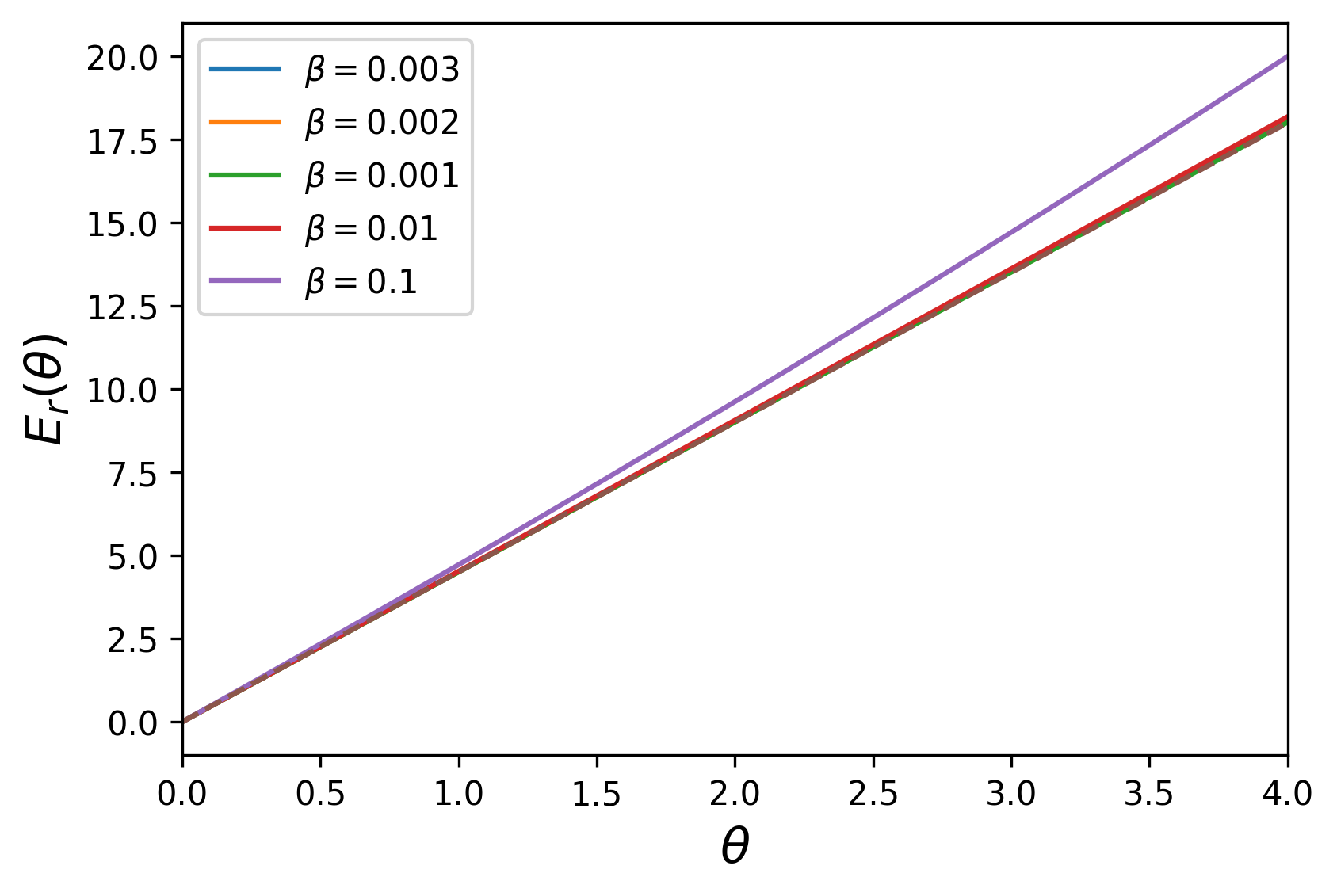
Figure 1: The neutral drift limit (brown dashed line) for the reward cost function $E_{r}(\theta)$ with $N=3$, $t=1$, and $\theta=1$ for DG with $B=2,c=1$. We notice that, the more the $\beta$ value approaches 0, the closer to the limiting value the cost function $E_{r}(\theta)$ gets, in accordance to the analytical result Proposition 1.

Proposition 2.

(Strong selection limit) It holds that

$$\lim\limits_{\beta\rightarrow\infty}E_{r}(\theta)=\begin{cases}+\infty\quad\text{if}\quad\delta+\theta>0,\\ \frac{2N^{2}\theta}{N-1}\quad\text{if}\quad\delta+\theta=0,\\ \frac{N^{2}\theta}{N-1}\quad\text{if}\quad\delta+\theta<0.\end{cases}$$

Proof.

We proceed as in the proof of the previous proposition by computing the limit of relevant quantities as $\beta\rightarrow\infty$ instead of $\beta\rightarrow 0$, noting that $\delta<0$ in our setting. We have

$$\lim\limits_{\beta\rightarrow\infty}d^{N-2}=\lim\limits_{\beta\rightarrow\infty}\left(\frac{1}{1+e^{\beta\delta}}\right)^{N-2}=1,$$

$$\lim\limits_{\beta\rightarrow\infty}(bd)=\lim\limits_{\beta\rightarrow\infty}\frac{1}{2+e^{\beta\delta}+e^{-\beta\delta}}=0,$$

$$\lim\limits_{\beta\rightarrow\infty}(ad)=\lim\limits_{\beta\rightarrow\infty}\frac{1}{(1+e^{\beta\delta})(1+e^{-\beta(\theta+\delta)})}=\begin{cases}1\quad\text{if}\quad\delta+\theta>0,\\ \frac{1}{2}\quad\text{if}\quad\delta+\theta=0,\\ 0\quad\text{if}\quad\delta+\theta<0.\end{cases}$$

It also follows that

$$\lim\limits_{\beta\rightarrow\infty}y_{2}=1,\quad\lim\limits_{\beta\rightarrow\infty}y_{3}=1.$$

Putting everything together yields

$$\lim_{\beta\rightarrow 0}E_{r}(\theta) =\lim_{\beta\rightarrow 0}\Bigg{(}\frac{N^{2}\theta}{2N-2}(1+\frac{d^{N-2}}{y_{2}})\Big{(}\frac{1}{1-ad\frac{y_{3}}{y_{2}}}\Big{)}\Bigg{)}$$

$$=\begin{cases}+\infty\quad\text{if}\quad\delta+\theta>0,\\ \frac{2N^{2}\theta}{N-1}\quad\text{if}\quad\delta+\theta=0,\\ \frac{N^{2}\theta}{N-1}\quad\text{if}\quad\delta+\theta<0.\end{cases}$$

∎

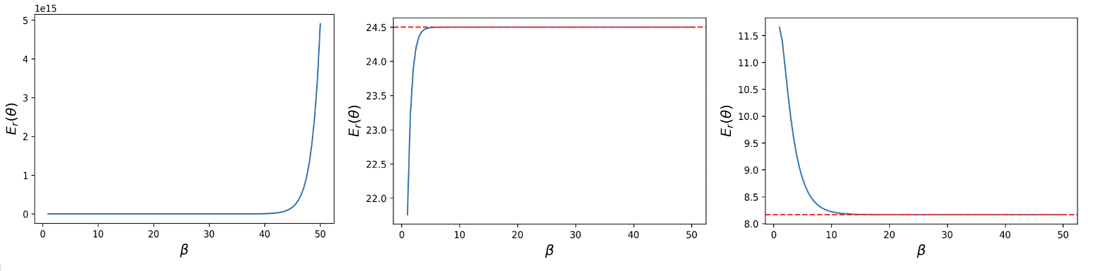
Figure 2: The strong selection limit (red dashed line) for the reward cost function $E_{r}(\theta)$ with $N=7$, $t=1$ for DG with $B=2,c=1$. The first image corresponds to $\delta+\theta>0$ ($\delta=-0.5$, $\theta=1$), the middle one to $\delta+\theta=0$ ($\delta=-1$, $\theta=1$), and the last one to $\delta+\theta<0$ ($\delta$ = -1.5, $\theta=1$). The numerical results are in accordance with the analytical one in Proposition 2.

4 Institutional Reward with $t=2$

In this section, we compute the reward cost function for $t=2$, i.e., when the institution provide rewards only if there are at most two cooperators in the population.

For $t=2$,

$W=\begin{pmatrix}1&-a&&&&&\\ -c&1&-a&&&&&\\ &-d&1&-b&&&\\ &&\ddots&\ddots&\ddots&\\ &&&-d&1&-b&&&\\ &&&&-d&1&-b&&&\\ &&&&&\ddots&\ddots&\ddots&\\ &&&&&&-d&1&-b\\ &&&&&&&-d&1\end{pmatrix}.$

Therefore, using Equation 3, we get

$$E_{r}(\theta) =\frac{N^{2}\theta}{2}\sum_{j=1}^{2}\frac{\left(W^{-1}\right)_{1,j}+\left(W^{-1}\right)_{N-1,j}}{N-j}$$

$$=\frac{N^{2}\theta}{2}\left[\left(\frac{\left(W^{-1}\right)_{1,1}+\left(W^{-1}\right)_{N-1,1}}{N-1}\right)+\left(\frac{\left(W^{-1}\right)_{1,2}+\left(W^{-1}\right)_{N-1,2}}{N-2}\right)\right].$$ (14)

To obtain a simplified version of Equation 4, we need to compute $(W^{-1})_{1,1}$, $(W^{-1})_{N-1,1}$, $(W^{-1})_{1,2}$, $(W^{-1})_{N-1,2}$. We apply Theorem 1, the diagonal element case, and Corollary 1, both cases, to get:

$$(W^{-1}_{1,1}) =\frac{1}{1-ac\frac{y_{3}}{y_{2}}},$$

$$(W^{-1})_{N-1,1} =cd^{N-3}\frac{1}{y_{2}}\frac{1}{1-ac\frac{y_{3}}{y_{2}}},$$

$$(W^{-1})_{1,2} =a\frac{1}{1-ac-ad\frac{y_{4}}{y_{3}}},$$

$$(W^{-1})_{N-1,2} =d^{N-3}\frac{1}{y_{3}}\frac{1}{1-ac-ad\frac{y_{4}}{y_{3}}}.$$

See Section 7.1 for detailed computations of the $W$ entries.

Substituting the $W$ values in Equation 4 yields:

$$E_{r}(\theta) =\frac{N^{2}\theta}{2}\left(\frac{\frac{1}{1-ac\frac{y_{3}}{y_{2}}}+cd^{N-3}\frac{1}{y_{2}}\frac{1}{1-ac\frac{y_{3}}{y_{2}}}}{N-1}+\frac{a\frac{1}{1-ac-ad\frac{y_{4}}{y_{3}}}+d^{N-3}\frac{1}{y_{3}}\frac{1}{1-ac-ad\frac{y_{4}}{y_{3}}}}{N-2}\right)$$

$$=\frac{N^{2}\theta}{2}\left[\frac{\frac{1}{1-ac\frac{y_{3}}{y_{2}}}\left(1+cd^{N-3}\cdot\frac{1}{y_{2}}\right)}{N-1}+\frac{\frac{1}{1-ac-ad\frac{y_{4}}{y_{3}}}\left(a+d^{N-3}\cdot\frac{1}{y_{3}}\right)}{N-2}\right].$$

5 Numerical Analysis

In this section, we present the results of our numerical analysis.

5.1 Behaviour of the cost functions

In the case of reward, punishment, and hybrid incentives, the cost functions $E_{r}(\theta)$, $E_{p}(\theta)$, and $E_{mix}(\theta)$ are increasing for all $1\leq t<N-1$ and become non-monotonic for $t=N-1$, exhibiting a phase transition. This behaviour is further accentuated by changes in the strength of selection, $\beta$. The larger this parameter is, the more pronounced the non-monotonic behaviour of the function becomes, as observed in Figures 3, 4, 5, 6. The aforementioned behaviour is robust to changes in the game-specific values such as $B$, $c$, $r$, $n$.

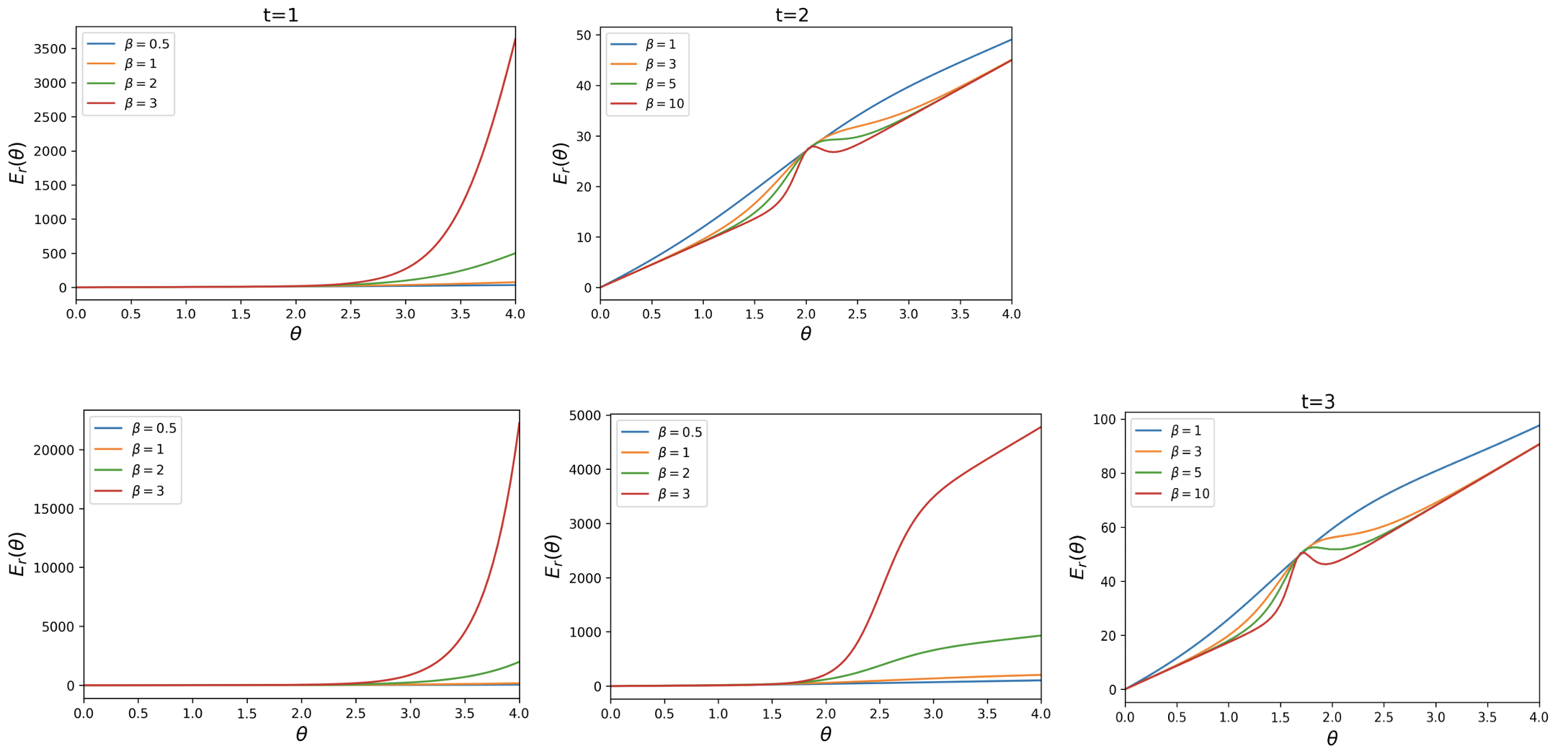
Figure 3: Behaviour of the reward cost function $E_{r}(\theta)$, for different thresholds $t$ and strengths of selection $\beta$, for DG with $B=2,c=1$. The first row corresponds to $N=3$ and the second one to $N=4$. The leftmost column corresponds to $t=1$, the middle one to $t=2$, the rightmost one to $t=3$.

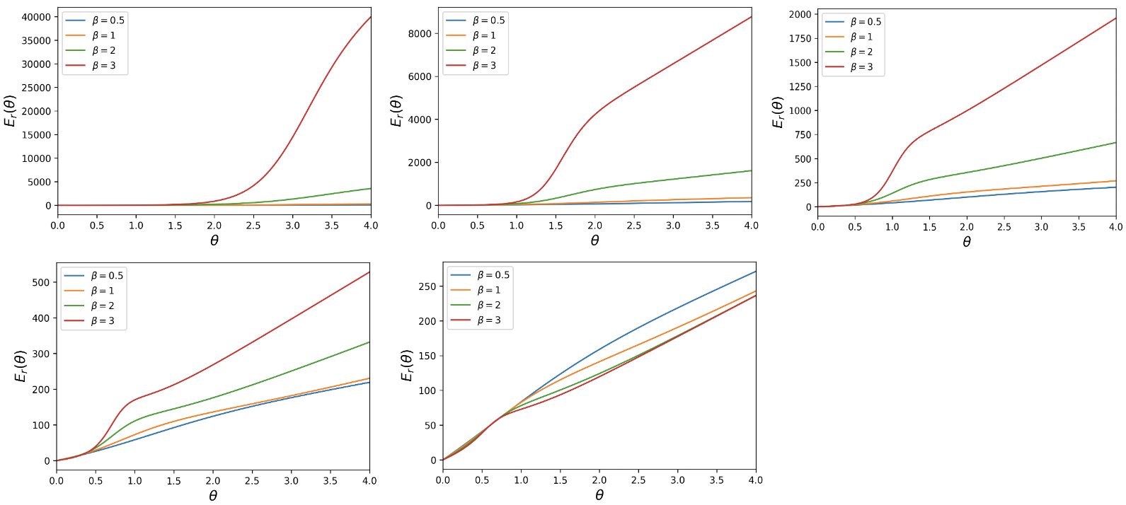
Figure 4: Behaviour of the reward cost function $E_{r}(\theta)$, for different thresholds $t$ and strengths of selection $\beta$, for PGG with $N=6,c=1,r=2,n=3$. The first row corresponds to $t=1$, $t=2$, and $t=3$, while the second one to $t=4$ and $t=5$.

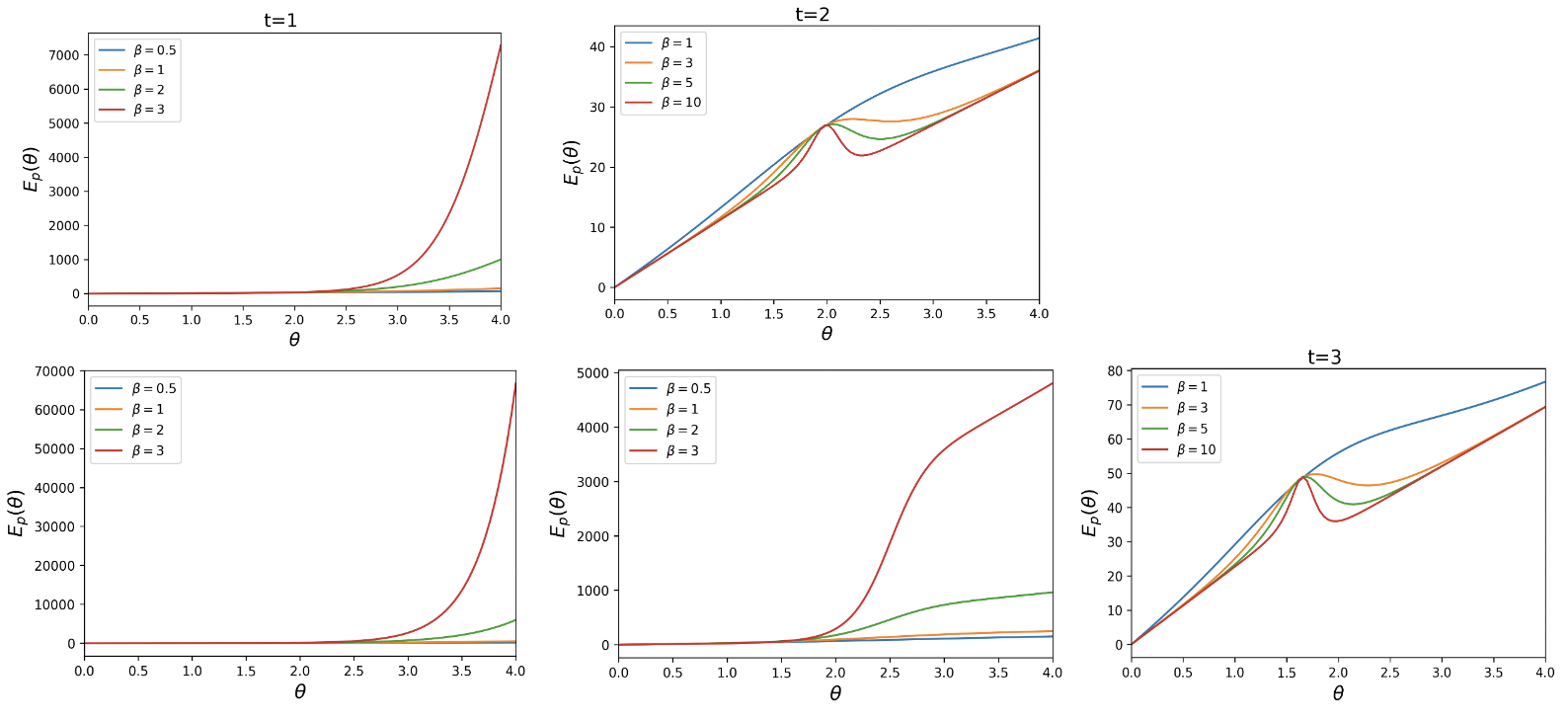
Figure 5: Behaviour of the punishment cost function $E_{p}(\theta)$, for different thresholds $t$ and strengths of selection $\beta$, for DG with $B=2,c=1$. The first row corresponds to $N=3$ and the second one to $N=4$. The leftmost column corresponds to $t=1$, the middle one to $t=2$, the rightmost one to $t=3$. The behaviour of the cost function for PGG is similar.

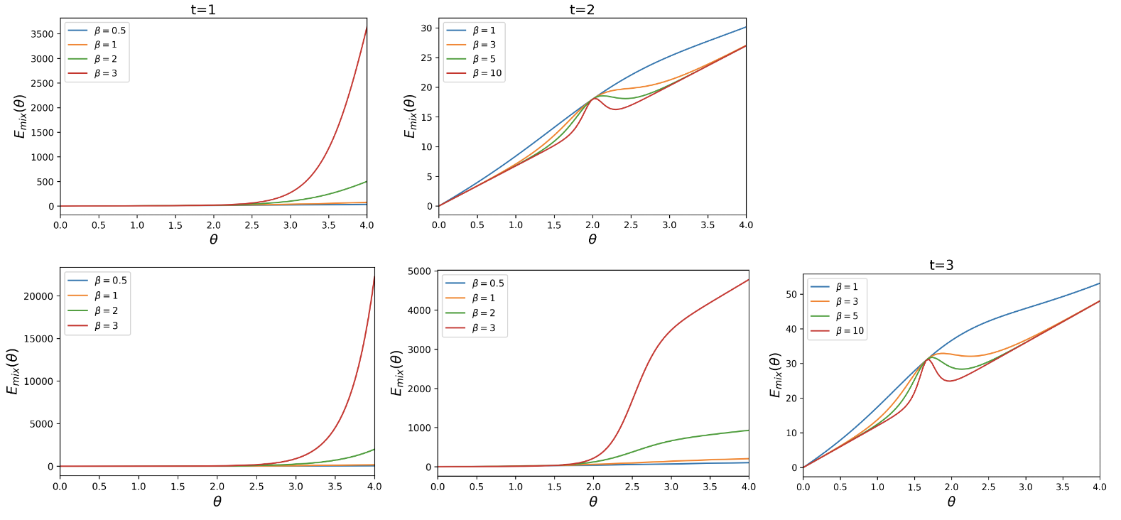
Figure 6: Behaviour of the mixed incentive (reward and punishment) cost function $E_{mix}(\theta)$ (where $a=1,b=1$), for different thresholds $t$ and strengths of selection $\beta$, for DG with $B=2,c=1$. The first row corresponds to $N=3$ and the second one to $N=4$. The leftmost column corresponds to $t=1$, the middle one to $t=2$, the rightmost one to $t=3$. The behaviour of the cost function for PGG is similar.

5.2 Phase transition: change in the qualitative behaviour of the cost function

Theorem 2 shows that the cost function $E(\theta)$ (either for reward, punish, or mixed incentives) for $t=1$ is always non-decreasing for all values of the intensity of selection $\beta$. In [5] it is shown that, for $t=N-1$, $E(\theta)$ is non-decreasing when $\beta$ is sufficiently small, but is not monotonic when $\beta$ is large enough. This demonstrates that the qualitative behaviour of the cost function changes significantly when $t$ and $\beta$ vary. We conjecture that there exists a critical threshold value of $t^{*}$ such that: for $t\leq t^{*}$, $E(\theta)$ is always non-deceasing for all $\beta$ when $t\leq t^{*}$, while for $t^{*}<t\leq N-1$, $E(\theta)$ is non-decreasing when $\beta$ is sufficiently small, but is not monotonic when $\beta$ is sufficiently large. Figures 3 - 6 suggest that for small population size $N$, the critical threshold $t^{*}$ is $N-1$. How to prove this interesting phase transition phenomena for general $N$ is elusive to us at the moment and deserves further investigation in the future.

All the simulations in Section 5 can be found in the ‘Evolutionary Game Theory’ repository under the Reward and Punishment - General t’ folder.

6 Discussion

Over the past decades, there has been a lot of attention given to studying effective incentive mechanisms with the aim of promoting cooperation. Various mechanisms have been tested [16, 25, 19, 20, 30], with some of the most efficient ones being institutional incentives, where there is a central decision-maker in charge of applying them. In our model, we adopt this idea of an external decision-maker and entrust them with providing reward, punishment, or hybrid incentives to players interacting via two cooperation dilemmas, the Donation Game or the Public Goods Game. While other works have examined a comparable setting, relatively few have looked at the question of optimising the overall cost to the institution while maintaining a certain degree of cooperation. Moreover, most studies have focused on the full-invest approach (also known as standard institutional incentive models), in which incentives are always provided regardless of the population composition.

In this paper, we studied the problem of optimising the cost of institutional incentives that are provided conditionally on the number of cooperators in the population (namely, when less than a threshold $t$) while guaranteeing a certain level of cooperation in a well-mixed, finite population of selfish individuals. We use mathematical analysis to derive the cost function as well as the neutral drift and strong selection limits for the case $t=1$ and the cost function for the case $t=2$. We provide numerical investigation for the aforementioned cases as well as for the others, i.e., for $2\leq t<N-1$.

For the mathematical analysis of the reward incentive cost function to be possible, we made some assumptions. Firstly, in order to derive the analytical formula for the frequency of cooperation, we assumed a small mutation limit [22, 17, 25]. Despite the simplified assumption, this small mutation limit approach has wide applicability to scenarios which go well beyond the strict limit of very small mutation rates [36, 11, 26, 21, 5]. If we were to relax this assumption, the derivation of a closed form for the frequency of cooperation would be intractable. Secondly, we focused on two important cooperation dilemmas, the Donation Game and the Public Goods Game. Both have in common that the difference in average payoffs between a cooperator and a defector does not depend on the population composition. This special property allowed us to simplify the fundamental matrix of the Markov chain to a tri-diagonal form and apply the techniques of matrix analysis [12] to obtain a closed form of its inverse matrix. In games with more complex payoff matrices such as the general prisoners’ dilemma and the collective risk game [27], this property no longer holds (e.g., in the former case the payoff difference, $\Pi_{C}(i)-\Pi_{D}(i)$, depends additively on $i$) and the technique in this paper cannot be directly applied. In these scenarios, we might consider other approaches to approximate the inverse matrix, exploiting its block structure.

We intend to utilise analytical techniques to explore the optimisation problem of punishment and hybrid incentives (reward and punishment used concurrently) for the individual-based incentive scheme. This would be interesting because it would allow for a cost comparison between reward or punishment incentives for a certain threshold value $t$ and the mixed scheme for the same value of $t$. Finally, there has been little attention given to the use of analysis for obtaining insights into cost-efficient incentives in structured populations or in more complex games (such as the general prisoners’ dilemma and the collective risk game), so this would also be an engaging research avenue.

7 Appendix

In this appendix, we provide explicit computations for the derivative of the reward cost function $E_{r}(\theta)$ for $t=1$ as well as small population examples for the reward case. We also include the computation of the $W$ entries for reward $t=2$.

7.1 The $W$ entries for the Reward cost function for $t=2$

$$(W^{-1}_{1,1}) =\frac{1}{1-(-c)(-a)\frac{y_{3}}{y_{2}}}$$

$$=\frac{1}{1-ac\frac{y_{3}}{y_{2}}},$$

$$(W^{-1})_{N-1,1} =(-1)^{N-2}\left(\prod_{k=1}^{N-2}a_{k+1}\right)\frac{y_{N}}{y_{2}}\phi_{1,1}$$

$$=(-1)^{N-2}\Bigg{(}\prod_{k=1}^{N-2}a_{k+1}\Bigg{)}\frac{1}{y_{2}}\frac{1}{1-ac\frac{y_{3}}{y_{2}}}$$

$$=(-1)^{N^{-2}}\left(a_{2}\cdot a_{3}\cdot\ldots\cdot a_{N-1}\right)\frac{1}{y_{2}}\frac{1}{1-a_{c}\frac{y_{3}}{y_{2}}}$$

$$=(-1)^{N-2}(-c)\cdot(-d)\cdot\ldots\cdot(-d)\frac{1}{y_{2}}\frac{1}{1-ac\frac{y_{3}}{y_{2}}}$$

$$=(-1)^{N-2}(-c)(-d)^{N-3}\frac{1}{y_{2}}\frac{1}{1-ac\frac{y_{3}}{y_{2}}}$$

$$=cd^{N-3}\frac{1}{y_{2}}\frac{1}{1-ac\frac{y_{3}}{y_{2}}},$$

$$(W^{-1})_{1,2} =(-1)^{1}\left(\prod_{k=1}^{1}c_{2-k}\right)\frac{z_{0}}{z_{1}}\phi_{2,2}$$

$$=-\left(c_{1}\right)\frac{1}{1}\phi_{2,2}$$

$$=a\phi_{2,2}$$

$$=a\frac{1}{1-(-c)(-a)\frac{z_{0}}{z_{1}}-(-d)(-a)\frac{y_{4}}{y_{3}}}$$

$$=a\frac{1}{1-ac-ad\frac{y_{4}}{y_{3}}},$$

$$(W^{-1})_{N-1,2} =(-1)^{N-3}\left(\prod_{k=1}^{N-3}a_{2+k}\right)\frac{y_{N}}{y_{3}}\phi_{2,2}$$

$$=(-1)^{N-3}\left(a_{3}\cdot a_{4}\ldots\cdot a_{N-1}\right)\frac{1}{y_{3}}\frac{1}{1-ac-ad\frac{y_{4}}{y_{3}}}$$

$$=(-1)^{N-3}(-d)^{N-3}\frac{1}{y_{3}}\frac{1}{1-ac-ad\frac{y_{4}}{y_{3}}}$$

$$=d^{N-3}\frac{1}{y_{3}}\frac{1}{1-ac-ad\frac{y_{4}}{y_{3}}}.$$

7.2 Small population examples for Reward

7.2.1 $N=3,t=1$

For $N=3,t=1$, we have

$$W=\begin{pmatrix}1&-a\\ -d&1\\ \end{pmatrix}$$

and

$$W^{-1}=\begin{pmatrix}\frac{-1}{ad-1}&\frac{-a}{ad-1}\\ \frac{-d}{ad-1}&\frac{-1}{ad-1}\\ \end{pmatrix}.$$

Thus, the cost function is

$$E_{r}(\theta) =\frac{N^{2}\theta}{2}\sum_{j=1}^{1}\frac{(W^{-1})_{1j}+(W^{-1})_{N-1,j}}{N-j}$$

$$=\frac{9\theta}{4}(W^{-1}_{11}+W^{-1}_{21})$$

$$=\frac{9\theta}{4}\frac{-d-1}{ad-1}$$

$$=\frac{9\theta}{4}\Bigg{(}\frac{1}{1-\frac{1}{(1+e^{-x})(e^{y}+1)}}+\frac{1}{\Big{(}1-\frac{1}{(1+e^{-x})(e^{y}+1)}\Big{)}(e^{y}+1)}\Bigg{)},$$

where $x=\beta(\delta+\theta)$ and $y=\beta\delta$.

7.2.2 $N=3,t=2$

For $N=3$, $t=2$, we have

$$W=\begin{pmatrix}1&-a\\ -c&1\\ \end{pmatrix}$$

and

$$W^{-1}=\begin{pmatrix}\frac{-1}{ac-1}&\frac{-a}{ac-1}\\ \frac{-c}{ac-1}&\frac{-1}{ac-1}\\ \end{pmatrix}.$$

Hence, the cost function is

$$E_{r}(\theta) =\frac{N^{2}\theta}{2}\sum_{j=1}^{2}\frac{(W^{-1})_{1j}+(W^{-1})_{N-1,j}}{N-j}$$

$$=\frac{N^{2}\theta}{2}\big{[}\frac{(W^{-1}_{11}+W^{-1}_{21})}{2}+(W^{-1}_{12}+W^{-1}_{22})\big{]}$$

$$=\frac{9\theta}{4}\Big{(}\frac{-c-1}{ac-1}\Big{)}+\frac{9\theta}{2}\Big{(}\frac{-a-1}{ac-1}\Big{)}$$

$$=\frac{9\theta}{4}\Bigg{(}\frac{1}{1-\frac{1}{(1+e^{-x})(1+e^{x})}}+\frac{1}{\Big{(}1-\frac{1}{(1+e^{-x})(1+e^{x})}\Big{)}(1+e^{x})}\Bigg{)}$$

$$\qquad+\frac{9\theta}{2}\Bigg{(}\frac{1}{1-\frac{1}{(1+e^{-x})(1+e^{x})}}+\frac{1}{\Big{(}1-\frac{1}{(1+e^{-x})(1+e^{x})}\Big{)}(1+e^{-x})}\Bigg{)},$$

where $x=\beta(\delta+\theta)$ and $y=\beta\delta$.

7.2.3 $N=4$, $t=1$

For $N=4$, $t=1$, we have

$$W=\begin{pmatrix}1&-a&0\\ -d&1&-b\\ 0&-d&1\\ \end{pmatrix}$$

and

$$W^{-1}=\begin{pmatrix}\frac{bd-1}{ad+bd-1}&\frac{-a}{ad+bd-1}&\frac{-ab}{ad+bd-1}\\ \frac{-d}{ad+bd-1}&\frac{-1}{ad+bd-1}&-\frac{-b}{ad+bd-1}\\ \frac{-d^{2}}{ad+bd-1}&\frac{-d}{ad+bd-1}&\frac{ad-1}{ad+bd-1}\\ \end{pmatrix}.$$

Thus, the cost function is

$$E_{r}(\theta) =\frac{N^{2}\theta}{2}\sum_{j=1}^{1}\frac{(W^{-1})_{1j}+(W^{-1})_{N-1,j}}{N-j}$$

$$=\frac{8\theta}{3}(W^{-1}_{11}+W^{-1}_{31})$$

$$=\frac{8\theta}{3}\frac{-d^{2}+bd-1}{ad+bd-1}$$

$$=\frac{8\theta}{3}\Bigg{(}\frac{-1+\frac{1}{(1+e^{-y})(e^{y}+1)}}{-1+\frac{1}{(1+e^{-y})(e^{y}+1)}+\frac{1}{(1+e^{-x})(e^{y}+1)}}-\frac{1}{(e^{y}+1)^{2}\Big{(}-1+\frac{1}{(1+e^{-y})(e^{y}+1)}+\frac{1}{(1+e^{-x})(e^{y}+1)}\Big{)}}\Bigg{)},$$

where $x=\beta(\delta+\theta)$ and $y=\beta\delta$.

7.2.4 $N=4$, $t=2$

For $N=4$, $t=2$, we have

$$W=\begin{pmatrix}1&-a&0\\ -c&1&-a\\ 0&-d&1\\ \end{pmatrix}$$

and

$$W^{-1}=\begin{pmatrix}\frac{ad-1}{ac+ad-1}&\frac{-a}{ac+ad-1}&\frac{-a^{2}}{ac+ad-1}\\ \frac{-c}{ac+ad-1}&\frac{-1}{ac+ad-1}&\frac{-a}{ac+ad-1}\\ \frac{-cd}{ac+ad-1}&\frac{-d}{ac+ad-1}&\frac{ac-1}{ac+ad-1}\\ \end{pmatrix}.$$

So the cost function is

$$E_{r}(\theta) =\frac{N^{2}\theta}{2}\sum_{j=1}^{2}\frac{(W^{-1})_{1j}+(W^{-1})_{N-1,j}}{N-j}$$

$$=8\theta\Bigg{[}\frac{(W^{-1}_{11}+W^{-1}_{31})}{3}+\frac{(W^{-1}_{12}+W^{-1}_{32})}{2}\Bigg{]}$$

$$=\frac{8\theta}{3}\Big{(}\frac{-cd+ad-1}{ac+ad-1}\Big{)}+4\theta\Big{(}\frac{-a-d}{ac+ad-1}\Big{)}$$

$$=\frac{8\theta}{3}\Bigg{(}\frac{-1+\frac{1}{(1+e^{-x})(e^{x}+1)}}{-1+\frac{1}{(1+e^{-x})(e^{y}+1)}+\frac{1}{(1+e^{-x})(e^{x}+1)}}-\frac{1}{(e^{x}+1)(e^{y}+1)\Big{(}-1+\frac{1}{(1+e^{-x})(e^{y}+1)}+\frac{1}{(1+e^{-x})(e^{x}+1)}\Big{)}}\Bigg{)}+$$

$$\qquad 4\theta\Bigg{(}\frac{1}{(e^{y}+1)\Big{(}1-\frac{1}{(1+e^{-x})(e^{y}+1)}-\frac{1}{(1+e^{-x})(e^{x}+1)}\Big{)}}-\frac{1}{(1+e^{-x})\Big{(}-1+\frac{1}{(1+e^{-x})(e^{y}+1)}+\frac{1}{(1+e^{-x})(e^{x}+1)}\Big{)}}\Bigg{)},$$

where $x=\beta(\delta+\theta)$ and $y=\beta\delta$.

7.2.5 $N=4$, $t=3$

For $N=4$, $t=3$, we have

$$W=\begin{pmatrix}1&-a&0\\ -c&1&-a\\ 0&-c&1\\ \end{pmatrix}$$

and

$$W^{-1}=\begin{pmatrix}\frac{ac-1}{2ac-1}&\frac{-a}{2ac-1}&\frac{-a^{2}}{2ac-1}\\ \frac{-c}{2ac-1}&\frac{-1}{2ac-1}&\frac{-a}{2ac-1}\\ \frac{-c^{2}}{2ac-1}&\frac{-c}{2ac-1}&\frac{ac-1}{2ac-1}\\ \end{pmatrix}.$$

Thus, the cost function is

$$E_{r}(\theta) =\frac{N^{2}\theta}{2}\sum_{j=1}^{3}\frac{(W^{-1})_{1j}+(W^{-1})_{N-1,j}}{N-j}$$

$$=\frac{N^{2}\theta}{2}\Bigg{[}\frac{(W^{-1}_{11}+W^{-1}_{31})}{3}+\frac{(W^{-1}_{12}+W^{-1}_{32})}{2}+(W^{-1}_{13}+W^{-1}_{33})\Bigg{]}$$

$$=\frac{8\theta}{3}\Big{(}\frac{c^{2}+ac-1}{2ac-1}\Big{)}+4\theta\Big{(}\frac{-a+c}{2ac-1}\Big{)}+8\theta\Big{(}\frac{-a^{2}+ac-1}{2ac-1}\Big{)}$$

$$=\frac{8\theta}{3}\Bigg{(}\frac{-1+\frac{1}{(1+e^{-x})(e^{x}+1)}}{-1+\frac{2}{(1+e^{-x})(e^{x}+1)}}-\frac{1}{\Big{(}1-\frac{2}{(1+e^{-x})(e^{x}+1)}\Big{)}(1+e^{x})^{2}}\Bigg{)}+$$

$$\qquad 4\theta\Bigg{(}\frac{1}{\Big{(}1-\frac{2}{(1+e^{-x})(e^{x}+1)}\Big{)}(e^{x}+1)}-\frac{1}{\Big{(}-1+\frac{2}{(1+e^{-x})(e^{x}+1)}\Big{)}(e^{-x}+1)}\Bigg{)}+$$

$$\qquad 8\theta\Bigg{(}\frac{-1+\frac{1}{(1+e^{-x})(e^{x}+1)}}{-1+\frac{2}{(1+e^{-x})(e^{x}+1)}}-\frac{1}{\Big{(}-1+\frac{2}{(1+e^{-x})(e^{x}+1)}\Big{)}(1+e^{-x})^{2}}\Bigg{)},$$

where $x=\beta(\delta+\theta)$ and $y=\beta\delta$.

Data Availability Statement

Data sharing is not applicable to this article as no datasets were generated or analysed during the current study.

References

• [1] Paul WB Atkins, David Sloan Wilson, and Steven C Hayes. Prosocial: Using evolutionary science to build productive, equitable, and collaborative groups. New Harbinger Publications, 2019.
• [2] Xiaojie Chen and Matjaž Perc. Optimal distribution of incentives for public cooperation in heterogeneous interaction environments. Frontiers in behavioral neuroscience, 8:248, 2014.
• [3] Theodor Cimpeanu, Cedric Perret, and The Anh Han. Cost-efficient interventions for promoting fairness in the ultimatum game. Knowledge-Based Systems, 233:107545, 2021.
• [4] Theodor Cimpeanu, Francisco C Santos, and The Anh Han. Does spending more always ensure higher cooperation? an analysis of institutional incentives on heterogeneous networks. Dynamic Games and Applications, pages 1–20, 2023.
• [5] M. H. Duong, C. M. Durbac, and T. A. Han. Cost optimisation of hybrid institutional incentives for promoting cooperation in finite populations. J. Math. Biol., 87(77), 2023.
• [6] Manh Hong Duong and The Anh Han. Cost efficiency of institutional incentives for promoting cooperation in finite populations. Proceedings of the Royal Society A, 477(2254):20210568, 2021.
• [7] António R. Góis, Fernando P. Santos, Jorge M. Pacheco, and Francisco C. Santos. Reward and punishment in climate change dilemmas. Sci. Rep., 9(1):1–9, 2019.
• [8] Özgür Gürerk, Bernd Irlenbusch, and Bettina Rockenbach. The competitive advantage of sanctioning institutions. Science (New York, N.Y.), 312:108–11, 05 2006.
• [9] The Anh Han, Simon Lynch, Long Tran-Thanh, and Francisco C Santos. Fostering cooperation in structured populations through local and global interference strategies. In Proceedings of the 27th International Joint Conference on Artificial Intelligence, pages 289–295, 2018.
• [10] The Anh Han and Long Tran-Thanh. Cost-effective external interference for promoting the evolution of cooperation. Scientific reports, 8(1):1–9, 2018.
• [11] Christoph Hauert, Arne Traulsen, Hannelore Brandt, Martin A. Nowak, and Karl Sigmund. Via freedom to coercion: The emergence of costly punishment. Science, 316(5833):1905–1907, 2007.
• [12] Y Huang and W F McColl. Analytical inversion of general tridiagonal matrices. Journal of Physics A: Mathematical and General, 30(22):7919, 1997.
• [13] Jim Kemeny. Perspectives on the micro-macro distinction. The Sociological Review, 24(4):731–752, 1976.
• [14] Linjie Liu and Xiaojie Chen. Effects of interconnections among corruption, institutional punishment, and economic factors on the evolution of cooperation. Applied Mathematics and Computation, 425:127069, 2022.
• [15] Martin A. Novak. Evolutionary Dynamics: Exploring the Equations of Life. Harvard University Press, 2006.
• [16] Martin A. Nowak. Five rules for the evolution of cooperation. Science, 314(5805):1560–1563, 2006.
• [17] Martin A. Nowak, Akira Sasaki, Christine Taylor, and Drew Fudenberg. Emergence of cooperation and evolutionary stability in finite populations. Nature, 428(6983):646–650, 2004.
• [18] Elinor Ostrom. Understanding institutional diversity. Princeton university press, 2005.
• [19] Matjaž Perc, Jillian J. Jordan, David G. Rand, Zhen Wang, Stefano Boccaletti, and Attila Szolnoki. Statistical physics of human cooperation. Physics Reports, 687:1–51, 2017.
• [20] David G. Rand and Martin A. Nowak. Human cooperation. Trends in cognitive sciences, 17(8):413–425, 2013.
• [21] David G Rand, Corina E. Tarnita, Hisashi Ohtsuki, and Martin A. Nowak. Evolution of fairness in the one-shot anonymous ultimatum game. Proceedings of the National Academy of Sciences, 110(7):2581–2586, 2013.
• [22] Bettina Rockenbach and Manfred Milinski. The efficient interaction of indirect reciprocity and costly punishment. Nature, 444:718–23, 01 2007.
• [23] Tatsuya Sasaki, Åke Brännström, Ulf Dieckmann, and Karl Sigmund. The take-it-or-leave-it option allows small penalties to overcome social dilemmas. Proceedings of the National Academy of Sciences, 109(4):1165–1169, 2012.
• [24] Tatsuya Sasaki, Xiaojie Chen, Åke Brännström, and Ulf Dieckmann. First carrot, then stick: How the adaptive hybridization of incentives promotes cooperation. Journal of the Royal Society Interface, 12:20140935, 01 2015.
• [25] Karl Sigmund. The calculus of selfishness. In The Calculus of Selfishness. Princeton University Press, 2010.
• [26] Karl Sigmund, Hannelore De Silva, Arne Traulsen, and Christoph Hauert. Social learning promotes institutions for governing the commons. Nature, 466:7308, 2010.
• [27] Weiwei Sun, Linjie Liu, Xiaojie Chen, Attila Szolnoki, and Vítor V Vasconcelos. Combination of institutional incentives for cooperative governance of risky commons. Iscience, 24(8), 2021.
• [28] Attila Szolnoki and Matja ž Perc. Second-order free-riding on antisocial punishment restores the effectiveness of prosocial punishment. Phys. Rev. X, 7:041027, Oct 2017.
• [29] Arne Traulsen and Martin A. Nowak. Evolution of cooperation by multilevel selection. Proceedings of the National Academy of Sciences, 103(29):10952–10955, 2006.
• [30] Paul A.M. Van Lange, Bettina Rockenbach, and Toshio Yamagishi. Reward and punishment in social dilemmas. Oxford University Press, 2014.
• [31] Shengxian Wang, Ming Cao, and Xiaojie Chen. Optimally combined incentive for cooperation among interacting agents in population games, 2023.
• [32] Shengxian Wang, Xiaojie Chen, and Attila Szolnoki. Exploring optimal institutional incentives for public cooperation. Communications in Nonlinear Science and Numerical Simulation, 79:104914, 2019.
• [33] Shengxian Wang, Xiaojie Chen, Zhilong Xiao, and Attila Szolnoki. Decentralized incentives for general well-being in networked public goods game. Applied Mathematics and Computation, 431:127308, 2022.
• [34] Shengxian Wang, Xiaojie Chen, Zhilong Xiao, Attila Szolnoki, and Vítor V Vasconcelos. Optimization of institutional incentives for cooperation in structured populations. Journal of the Royal Society Interface, 20(199):20220653, 2023.
• [35] Shengxian Wang, Linjie Liu, and Xiaojie Chen. Incentive strategies for the evolution of cooperation: Analysis and optimization. Europhysics Letters, 136(6):68002, 2021.
• [36] Ioannis Zisis, Sibilla Di Guida, The Anh Han, Georg Kirchsteiger, and Tom Lenaerts. Generosity motivated by acceptance-evolutionary analysis of an anticipation game. Scientific reports, 5(1):1–11, 2015.