Combining Evolutionary Strategies and Novelty Detection to go Beyond the Alignment Limit of the $Z_{3}$ 3HDM

Abstract

We present a novel Artificial Intelligence approach for Beyond the Standard Model parameter space scans by augmenting an Evolutionary Strategy with Novelty Detection. Our approach leverages the power of Evolutionary Strategies, previously shown to quickly converge to the valid regions of the parameter space, with a novelty reward to continue exploration once converged. Taking the $Z_{3}$ 3HDM as our Physics case, we show how our methodology allows us to quickly explore highly constrained multidimensional parameter spaces, providing up to eight orders of magnitude higher sampling efficiency when compared with pure random sampling and up to four orders of magnitude when compared to random sampling around the alignment limit. In turn, this enables us to explore regions of the parameter space that have been hitherto overlooked, leading to the possibility of novel phenomenological realisations of the $Z_{3}$ 3HDM that had not been considered before.

I Introduction

The Standard Model (SM) of particle physics has demonstrated remarkable success in accurately describing the electroweak and strong interactions. However, experimental challenges such as neutrino mass, dark matter, and the baryonic asymmetry of the Universe prompt the exploration of physics Beyond the SM (BSM). In many cases, BSM theories involve expanding the minimal scalar sector of the SM, characterised by a single Higgs doublet. Multi-Higgs doublet models are particularly prominent among these extensions, primarily because they maintain the tree-level value of the electroweak $\rho$-parameter, in good agreement with experimental observations. The extensively studied two Higgs doublet model (2HDM) [1] has provided valuable insights. More recently, there has been a surge of interest in the investigation of three Higgs doublet models (3HDMs) [2, 3, 4, 5, 6, 7, 8, 9, 10, 11, 12, 13, 14, 15, 16], where the scalar sector encompasses three Higgs doublets. These models show great promise as they possess the essential ingredients to address the challenges posed by dark matter and the baryonic asymmetry of the Universe.

With no unambiguous signs of New Physics in general and of extra exotic scalars in particular, BSM phenomenology is faced with an ever increasing and ever more restricting list of (direct and indirect) experimental constraints, in addition to any theoretical and self-consistency constraints. From a model building perspective, this means that the allowed regions of BSM parameter spaces are effectively shrinking, making finding such regions ever more difficult or outright impractical, even if those regions host points which are very good fits to the data. To mitigate this, BSM phenomenologists often simplify the problem in two possible ways. The first approach is to simplify the constraints and leave some questions unanswered, to be eventually addressed by an Ultra Violet completion. The second approach relies on simplifying the sampling space by changing the priors from which the parameters are drawn, usually by restricting the parameter space to a subregion where known valid points had been found before or for which there is a limiting case, such as the case of the alignment limit in multi Higgses models. While in the former case one ends up with an incomplete model, in the latter case one is left with the worrisome prospect of missing out possible phenomenological signatures.

In recent years, Artificial Intelligence (AI) in general, and Machine Learning (ML) in particular, have received considerable attention by the High Energy Physics (HEP) community with a wide range of applications [17]. Of particular interest to this work are the ongoing attempts to explore the parameter space of highly constrained and multidimensional BSM scenarios, where sampling points that respect theoretical and experimental bounds poses a great challenge. The first attempts to mitigate this problem using AI/ML are based on using supervised classifiers and regressors to produce estimates of BSM predictions of physical observables and physical quantities [18, 19, 20, 21, 22], bypassing the computational overhead often associated with these. Other approaches leverage the active learning framework to track the ground truth of the observables to draw the boundary of the allowed regions of the parameter space [23, 24]. However, we point out that the usage of AI/ML for BSM parameter spaces studies is not restricted to exploration, as generative models have been studied to provide a possible way of replicating points from valid regions [25] or to gain new insights through latent space visualisation [26].

The approaches cited above rely heavily on the quality of the trained ML model, namely on the coverage of the parameter space provided by the points used, especially in or near valid regions. A different approach was presented in [27], where different AI-based exploration algorithms were used to explore the parameter space of the cMSSM (four parameters) and the pMSSM (16 parameters) by reframing the problem as a black-box optimisation problem. In such an approach, exploration starts with just a few random points from which iterative algorithms will progressively suggest better points through trial and error. Although the Physics cases in [27] were not especially realistic, as only Higgs mass and Dark Matter relic density constraints were used, the methodology provided orders of magnitude of sampling efficiency improvement over random sampling, while still capturing a global picture of the parameter space.

In this paper, we will extend and build on top of that of [27]. In that work, an Evolutionary Strategy algorithm was observed to eagerly converge to the valid region of the parameter space and to stop exploring once converged. To mitigate this, in [27] the algorithm was endowed with a restart strategy to draw a more global picture of the valid region of the parameter space. In this work, we will take a different approach by incorporating a novelty reward into the black-box optimisation problem to drive the exploration algorithm away from the regions already explored. As we will see, our approach retains the benefits of drastically improving sampling efficiency while gaining a novel approach to charter the valid region of the parameter space.

Although the proposed approach is general to any BSM parameter space, we will use our novel methodology to perform a realistic search on the highly constrained $Z_{3}$ 3HDM model, where all known and possible constraints will be considered. This poses a terrific challenge for sampling valid points from the parameter space, which has led previous studies to consider sampling around the alignment limit. Therefore, the $Z_{3}$ 3HDM provides an ideal scenario not only to develop our methodology, but to use to do new Physics by exploring points beyond random sampling strategies around the alignment limit and to discover novel phenomenological realisations of the $Z_{3}$ 3HDM that have been obfuscated in the past such strategies.

This paper is organised as follows. In section II we present the $Z_{3}$ 3HDM model which is the Physics subject of our study. In section III we present its constraints, both theoretical and experimental. In section IV we outline the random sampling strategy near the alignment limit, which we will use to compare our methodology. In section V we introduce the AI scan strategy, redefining the scan as black-box optimisation, and the novelty award based on density estimation. In section VI we present and analyse the results obtained with our methodology, showcasing the versatility of our approach. Finally, in section VII we conclude our discussion and point out novel directions of work.

II The $Z_{3}$ 3HDM Model

II.1 Scalar Sector

For the potential of the $Z_{3}$ 3HDM model, denoted $V_{Z_{3}}$, we use the conventions of [6]. The $Z_{3}$-invariant terms, given by $\phi_{i}\to\phi_{i}^{\prime}=(S_{Z_{3}})_{ij}\phi_{j}$, can be expressed as:

$$V_{Z_{3}}=V_{2}+V_{4},$$ (1)

with the quartic part represented by:

$$V_{4} =\lambda_{1}(\phi_{1}^{\dagger}\phi_{1})^{2}+\lambda_{2}(\phi_{2}^{\dagger}\phi_{2})^{2}+\lambda_{3}(\phi_{3}^{\dagger}\phi_{3})^{2}+\lambda_{4}(\phi_{1}^{\dagger}\phi_{1})(\phi_{2}^{\dagger}\phi_{2})+\lambda_{5}(\phi_{1}^{\dagger}\phi_{1})(\phi_{3}^{\dagger}\phi_{3})$$

$$\quad+\lambda_{6}(\phi_{2}^{\dagger}\phi_{2})(\phi_{3}^{\dagger}\phi_{3})+\lambda_{7}(\phi_{1}^{\dagger}\phi_{2})(\phi_{2}^{\dagger}\phi_{1})+\lambda_{8}(\phi_{1}^{\dagger}\phi_{3})(\phi_{3}^{\dagger}\phi_{1})+\lambda_{9}(\phi_{2}^{\dagger}\phi_{3})(\phi_{3}^{\dagger}\phi_{2})$$

$$\quad+\left[\lambda_{10}(\phi_{1}^{\dagger}\phi_{2})(\phi_{1}^{\dagger}\phi_{3})+\lambda_{11}(\phi_{1}^{\dagger}\phi_{2})(\phi_{3}^{\dagger}\phi_{2})+\lambda_{12}(\phi_{1}^{\dagger}\phi_{3})(\phi_{2}^{\dagger}\phi_{3})+\text{h.c.}\right].$$ (2)

The quadratic part, denoted as $V_{2}$, is given by:

$$V_{2}=m_{11}^{2}\phi_{1}^{\dagger}\phi_{1}+m_{22}^{2}\phi_{2}^{\dagger}\phi_{2}+m_{33}^{2}\phi_{3}^{\dagger}\phi_{3}+\left[m_{12}^{2}(\phi_{1}^{\dagger}\phi_{2})+m_{13}^{2}(\phi_{1}^{\dagger}\phi_{3})+m_{23}^{2}(\phi_{2}^{\dagger}\phi_{3})+\text{h.c.}\right],$$ (3)

which includes terms, $m_{12}^{2}$, $m_{13}^{2}$, and $m_{23}^{2}$, responsible for breaking the symmetry softly.

Following spontaneous symmetry breaking (SSB), the three doublets can be parameterised in terms of their component fields as:

$$\phi_{i}=\begin{pmatrix}w_{k}^{\dagger}\\ (v_{i}+x_{i}+i\,z_{i})/\sqrt{2}\end{pmatrix}\,\,,\qquad(i=1,2,3)$$ (4)

where $v_{i}/\sqrt{2}$ corresponds to the vacuum expectation value (vev) for the neutral component of $\phi_{i}$. It is assumed that the scalar sector of the model explicitly and spontaneously conserves CP. Under this assumption, all parameters in the scalar potential are real, and the vevs $v_{1}$, $v_{2}$, $v_{3}$ are also real.

The scalar potential in eq. 1 contains eighteen parameters, and the vevs are parameterised as follows:

$$v_{1}=v\cos\beta_{1}\cos\beta_{2}\,,\qquad v_{2}=v\sin\beta_{1}\cos\beta_{2}\,,\qquad v_{3}=v\sin\beta_{2},$$ (5)

leading to the Higgs basis [28, 29, 30] obtained by the following rotation,

$$\begin{pmatrix}H_{0}\\ R_{1}\\ R_{2}\end{pmatrix}=\mathcal{O}_{\beta}\begin{pmatrix}x_{1}\\ x_{2}\\ x_{3}\end{pmatrix}=\begin{pmatrix}c_{\beta_{2}}c_{\beta_{1}}&c_{\beta_{2}}s_{\beta_{1}}&s_{\beta_{2}}\\ -s_{\beta_{1}}&c_{\beta_{1}}&0\\ -c_{\beta_{1}}s_{\beta_{2}}&-s_{\beta_{1}}s_{\beta_{2}}&c_{\beta_{2}}\end{pmatrix}\begin{pmatrix}x_{1}\\ x_{2}\\ x_{3}\end{pmatrix},$$ (6)

where here we have used the short notation, $c_{x}\equiv\cos x,s_{x}\equiv\sin x$.

Orthogonal matrices, denoted as R, P and Q, diagonalise the squared mass matrices in the CP-even scalar, CP-odd scalar, and charged scalar sectors. These matrices are crucial for transforming the weak basis into the physical mass basis for states with well-defined masses. Although this has already been discussed before [6, 10, 31], for completeness and to fix our notation, we give here the rotations that relate the mass eigenstates to the weak basis states.

For the neutral scalar sector, the mass terms can be extracted through the following rotation,

$$\begin{pmatrix}h_{1}\\ h_{2}\\ h_{3}\end{pmatrix}=\mathcal{O}_{\alpha}\begin{pmatrix}x_{1}\\ x_{2}\\ x_{3}\end{pmatrix},$$ (7)

where we take $h_{1}\equiv h_{125}$ to the be the 125 GeV Higgs boson found at LHC. The form chosen for $\mathcal{O}_{\alpha}\equiv\textbf{R}$ is

$$\textbf{R}\equiv\mathcal{O}_{\alpha}=\mathcal{R}_{3}.\mathcal{R}_{2}.\mathcal{R}_{1},$$ (8)

where the matrices $\mathcal{R}_{i}$ are

$$\mathcal{R}_{1}=\begin{pmatrix}c_{\alpha_{1}}&s_{\alpha_{1}}&0\\ -s_{\alpha_{1}}&c_{\alpha_{1}}&0\\ 0&0&1\end{pmatrix}\,,\quad\mathcal{R}_{2}=\begin{pmatrix}c_{\alpha_{2}}&0&s_{\alpha_{2}}\\ 0&1&0\\ -s_{\alpha_{2}}&0&c_{\alpha_{2}}\end{pmatrix}\,,\quad\mathcal{R}_{3}=\begin{pmatrix}1&0&0\\ 0&c_{\alpha_{3}}&s_{\alpha_{3}}\\ 0&-s_{\alpha_{3}}&c_{\alpha_{3}}\end{pmatrix}\,.\quad$$ (9)

For the charged and pseudoscalar sectors, the physical scalars can be obtained via the following $3\times 3$ rotations,

$$\begin{pmatrix}G^{0}\\ A_{1}\\ A_{2}\end{pmatrix}=\mathcal{O}_{\gamma_{1}}\mathcal{O}_{\beta}\begin{pmatrix}z_{1}\\ z_{2}\\ z_{3}\end{pmatrix},\qquad\begin{pmatrix}G^{+}\\ H_{1}^{+}\\ H_{2}^{+}\end{pmatrix}=\mathcal{O}_{\gamma_{2}}\mathcal{O}_{\beta}\begin{pmatrix}w_{1}^{\dagger}\\ w_{2}^{\dagger}\\ w_{3}^{\dagger}\end{pmatrix},$$ (10)

where, the rotation matrices are given by

$$\mathcal{O}_{\gamma_{1}}=\begin{pmatrix}1&0&0\\ 0&c_{\gamma_{1}}&-s_{\gamma_{1}}\\ 0&s_{\gamma_{1}}&c_{\gamma_{1}}\end{pmatrix},\qquad\mathcal{O}_{\gamma_{2}}=\begin{pmatrix}1&0&0\\ 0&c_{\gamma_{2}}&-s_{\gamma_{2}}\\ 0&s_{\gamma_{2}}&c_{\gamma_{2}}\end{pmatrix}.$$ (11)

For later use, we define the matrices P and Q as the combinations that connect the weak basis to the physical mass basis for the CP odd and charged Higgs scalars, respectively,

$$\textbf{P}\equiv\mathcal{O}_{\gamma_{1}}\mathcal{O}_{\beta},\qquad\textbf{Q}\equiv\mathcal{O}_{\gamma_{2}}\mathcal{O}_{\beta}.$$ (12)

As the states in the physical basis have well-defined masses, we can obtain relations between the set

$$\left\{v,\beta_{1},\beta_{2},m_{h1},m_{h2},m_{h3},m_{A1},m_{A2},m_{H_{1}^{\pm}},m_{H_{2}^{\pm}},\alpha_{1},\alpha_{2},\alpha_{3},\gamma_{1},\gamma_{2}\right\},$$ (13)

and the potential parameters in eq. 1, as shown in Ref. [6, 10, 31].

II.2 Higgs-Fermion Yukawa Interactions

In the Type-I models considered here, fermion fields are unaffected by the $Z_{3}$ transformation, allowing them to couple only to $\phi_{3}$. The Yukawa couplings to fermions are expressed compactly as:

$$\mathscr{L}_{\rm Y}\ni-\frac{m_{f}}{v}\bar{f}(a^{f}_{j}+i\,b^{f}_{j}\gamma_{5})fh_{j},$$ (14)

where $h_{j}\equiv(h_{1},h_{2},h_{3},A_{1},A_{2})_{j}$ represents the physical Higgs fields. For completeness, we list the couplings $a_{j}^{f}$ and $b_{j}^{f}$ here [12]. We have,

$$a_{j}^{f}\to \frac{\textbf{R}_{j,3}}{\hat{v_{3}}},\qquad\qquad j=1,2,3\qquad\text{for all leptons and down quarks},$$

$$b_{j}^{f}\to \frac{\textbf{P}_{j-2,3}}{\hat{v_{3}}},\qquad\quad j=4,5\quad\qquad\text{for all leptons and down quarks},$$

$$a_{j}^{f}\to \frac{\textbf{R}_{j,3}}{\hat{v_{3}}},\qquad\qquad j=1,2,3\qquad\text{for all up quarks},$$

$$b_{j}^{f}\to -\frac{\textbf{P}_{j-2,3}}{\hat{v_{3}}},\quad\quad j=4,5\quad\qquad\text{for all up quarks},$$ (15)

For the charged Higgs, $H_{1}^{\pm}$ and $H_{2}^{\pm}$, the Yukawa couplings to fermions are expressed as:

$$\mathscr{L}_{\rm Y} \ni \frac{\sqrt{2}}{v}\bar{\psi}_{d_{i}}\left[m_{\psi_{d_{i}}}V_{ji}^{\ast}\,\eta_{k}^{L}P_{L}+m_{\psi_{u_{j}}}V_{ji}^{\ast}\,\eta_{k}^{R}P_{R}\right]\psi_{u_{j}}H_{k}^{-}$$ (16)

$$+\frac{\sqrt{2}}{v}\bar{\psi}_{u_{i}}\left[m_{\psi_{d_{j}}}V_{ij}\,\eta_{k}^{L}P_{R}+m_{\psi_{u_{i}}}V_{ij}\,\eta_{k}^{R}P_{L}\right]\psi_{d_{j}}H_{k}^{+},$$

where $(\psi_{u_{i}},\psi_{d_{i}})$ is $(u_{i},d_{i})$ for quarks or $(\nu_{i},\ell_{i})$ for leptons. The coefficients $\eta_{k}^{\ell\,L}$, $\eta_{k}^{\ell\,R}$, $\eta_{k}^{q\,L}$, and $\eta_{k}^{q\,R}$ are

$$\eta_{k}^{\ell\,L}=-\frac{\textbf{Q}_{k+1,3}}{\hat{v_{3}}}\,,\quad\eta_{k}^{\ell\,R}=0\,,\quad\eta_{k}^{q\,L}=-\frac{\textbf{Q}_{k+1,3}}{\hat{v_{3}}}\,,\quad\eta_{k}^{q\,R}=\frac{\textbf{Q}_{k+1,3}}{\hat{v_{3}}}\,,\quad\text{k=1,2}\,.$$ (17)

III Constraints

In this section, we outline the various constraints necessary to impose theoretical and phenomenological consistency on the model parameters. The specifics of these constraints in the context of 3HDM are well established, as documented in previous works [10, 12, 16]. For brevity, we provide a brief list here, deferring further elaboration to appendix A.

From a phenomenological standpoint, our primary objective is to ensure the existence of an SM-like Higgs, identifiable as the scalar boson detected at the LHC. As demonstrated in [6], achieving this involves staying close to the ’alignment limit,’ characterised in the 3HDM by the conditions:

$$\alpha_{1}=\beta_{1}\,,\qquad\alpha_{2}=\beta_{2}\,.$$ (18)

In this limit, the lightest CP-even scalar, denoted as $h$, exhibits exact SM-like couplings at the tree level, automatically satisfying constraints from Higgs signal strengths. However, our interest lies in exploring permissible deviations from this precise alignment. To this end, we use the signal strength formalism, comparing the results with the experimental limits [32].

Subsequently, we must address constraints stemming from electroweak precision parameters, specifically $S$, $T$, and $U$. We use the analytic expressions of Ref.[33], contrasting them with the fit values provided in Ref.[34]. Notably, similar to the 2HDM scenario, we can bypass $T$-parameter constraints by imposing [14]:

$$m_{C1}=m_{A1}\,,\qquad m_{C2}=m_{A2}\,,\qquad\gamma_{1}=\gamma_{2}\,.$$ (19)

as we will explain in section IV.

Additionally, we incorporate constraints arising from flavour data, as detailed in appendix A. Direct searches at the LHC for the heavy non-standard scalars are also considered, employing HiggsTools-1.1.3 following Ref. [35], which provides a comprehensive list of relevant experimental searches.

For theoretical constraints, we insist on the perturbativity of Yukawa couplings, perturbative unitarity, and BFB (bounded from below) conditions. The implementation details for these constraints can be found in appendix A.

IV Random Scan strategy

We developed a dedicated code specifically for the $Z_{3}$ constrained 3HDM , building upon our earlier codes [38, 39, 10]. A thorough exploration of the parameter space was conducted using eq. 13. Our fixed inputs remained $v=246,\text{GeV}$ and $m_{h1}=125,\text{GeV}$. Random values were assigned within the following ranges:

$$\alpha_{1}\,,\alpha_{2}\,,\alpha_{3}\,,\gamma_{1}\,,\gamma_{2},\in\left[-\frac{\pi}{2},\frac{\pi}{2}\right];\qquad\tan{\beta_{1}}\,,\tan{\beta_{2}},\in\left[0.3,10\right];$$

$$m_{H_{1}}\equiv m_{h_{2}}\,,m_{H_{2}}\equiv m_{h_{3}},\in\left[125,1000\right],\text{GeV};$$ (20)

$$m_{A_{1}}\,,m_{A_{2}},m_{H_{1}^{\pm}}\,,m_{H_{2}^{\pm}},\in\left[100,1000\right],\text{GeV};$$ (21)

$$m^{2}_{12},m^{2}_{13},m^{2}_{23}\in\left[\pm 10^{-1},\pm 10^{7}\right],\text{GeV}^{2}\,,$$ (22)

where the last expression applies only to the soft masses that are not obtained as derived quantities (see Ref.[10] for the complete expressions).

However, this extensive scan exhibited low efficiency (as detailed in table 3 below). Recognising the significance of alignment in 3HDM [6, 10, 9], where alignment is defined by the lightest Higgs scalar having Standard Model (SM) couplings, we imposed constraints to enhance efficiency. Initially, aligning $\alpha_{1}$ with $\beta_{1}$ and $\alpha_{2}$ with $\beta_{2}$ (eq. 18) did not yield enough good points. Ref. [9] introduced an additional condition :

$$\gamma_{1}=\gamma_{2}=-\alpha_{3},\quad m_{H_{1}}=m_{A_{1}}=m_{H_{1}^{\pm}},\quad m_{H_{2}}=m_{A_{2}}=m_{H_{2}^{\pm}},$$ (23)

This, alongside eq. 18, led to a symmetric form of the quartic part of the potential[40, 9]. In fact, these conditions simplified the potential to

$$V_{\rm Sym,Lim}=\lambda_{\rm SM}\left[(\phi_{1}^{\dagger}\phi_{1})+(\phi_{2}^{\dagger}\phi_{2})+(\phi_{3}^{\dagger}\phi_{3})\right]^{2}\,,$$ (24)

where

$$\lambda_{\rm SM}=\frac{m_{h}^{2}}{2v^{2}},$$ (25)

is the the SM quartic Higgs coupling. All $\lambda_{i}$ vanish or are expressed in terms of $\lambda_{\rm SM}$. The validity of eq. 18 and  eq. 23 also implies that the soft masses can be explicitly solved, that is, they are no more independent parameters (see Ref.[10] for complete expressions). Now it should be clear why all such points are good points. Due to alignment, the LHC results on the $h_{125}$ are easily obeyed, whereas the perturbativity unitarity, STU and the other constraints are automatically obeyed.

To facilitate efficiency and consider deviations from strict alignment, two conditions were introduced [10]. The first denoted ”Al-1”, allowed a percentage deviation:

$$\frac{\alpha_{1}}{\beta_{1}},\frac{\alpha_{2}}{\beta_{2}},\in,[0.5,1.5]\,.\ \ \ \textbf{(Al-1)}$$ (26)

The condition ”Al-2” was more stringent, combining Al-1 with six additional conditions:

$$\frac{\alpha_{1}}{\beta_{1}},\frac{\alpha_{2}}{\beta_{2}},\frac{\gamma_{2}}{\gamma_{1}},\frac{-\alpha_{3}}{\gamma_{1}},\frac{m_{A_{1}}}{m_{H_{1}}},\frac{m_{H_{1}^{\pm}}}{m_{H_{1}}},\frac{m_{A_{2}}}{m_{H_{2}}},\frac{m_{H_{2}^{\pm}}}{m_{H_{2}}},\in,[0.5,1.5]\,.\ \ \ \textbf{(Al-2)}$$ (27)

These conditions, especially Al-2, improved the generation of meaningful points beyond the SM, even with a departure from strict alignment.

V Artificial Intelligence Black-Box Optimiser Scan Strategy

To quickly explore the parameter space, we will employ the AI black box optimisation approach to parameter space sampling first presented in [27]. In this approach, a constraint function, $C$, is introduced,

$$C(\mathcal{O})=\max(0,-\mathcal{O}+\mathcal{O}_{LB},\mathcal{O}-\mathcal{O}_{UB})\,,$$ (28)

where $\mathcal{O}$ is the value of an observable (or a constrained quantity), $\mathcal{O}_{LB}$ is its lower bound (i.e. its lowest allowed value), and $\mathcal{O}_{UB}$ its upper bound (i.e. its highest allowed value). Here, $\mathcal{O}$ is obtained by some computational routine that maps the parameter space to physical quantities, where the details of such routine are irrelevant and can therefore be taken as a black-box. If the value of $\mathcal{O}$ is within its lower and upper bounds, $C(\mathcal{O})$ returns $0$, otherwise it returns a positive number that measures how far the value of $\mathcal{O}$ is from its allowed interval. $\mathcal{O}$ is dependent on the parameters of the model, $\theta=(\alpha_{1},\beta_{1},\dots)\in\mathcal{P}$ (where $\mathcal{P}$ is the parameter space defined by eq. 22), that is, $\mathcal{O}=\mathcal{O}(\theta)$, which implies that $C(\mathcal{O})=C(\mathcal{O}(\theta))=C(\theta)$. Therefore, the set of valid points, $\mathcal{V}$, that satisfy a constraint can be defined in terms of $\theta$ as

$$\mathcal{V}=\left\{\theta^{*}:\ \theta\in\mathcal{P}\text{ s.t. }C(\theta)=0\right\}\ .$$ (29)

Since $C(\theta)$ is both vanishing and minimal in $\mathcal{V}$, the same set can be defined through the optimisation statement

$$\mathcal{V}=\left\{\theta^{*}:\ \theta\in\mathcal{P}\text{ s.t. }\theta^{*}=\arg\min C(\theta)\right\}\ .$$ (30)

Therefore, the task of finding the points in the parameter space that satisfy constraints is the same as finding the points that minimise $C(\mathcal{O})$. When faced with multiple constraints on multiple observables or constrained quantities, $\mathcal{O}_{i}$, we can then combine them into a single loss function, $L$, which we wish to minimise

$$L(\theta)=\sum_{i=1}^{N_{C}}C(\mathcal{O}_{i}(\theta)),$$ (31)

where the sum runs over all the $N_{C}$ constraints discussed in section III, and $L\geq 0\ \forall_{\theta}$ with $L=0$ if and only if all constraints are met. We notice that the quantity $\mathcal{O}_{i}$ does not need to be observable, such as the $\mu_{if}$ signal strengths measured by the LHC. For example, the theoretical constraints related to BFB and unitary conditions are included as $\mathcal{O}_{i}$ with the respective required bounds. The ability to mix measurements, limits, and theoretical constraints in the same loss function is a key strength of this methodology. Although $\mathcal{O}_{i}$ included observables and other constrained quantities, we will often abuse terminology and refer to all $\mathcal{O}_{i}$ as observables and the space they span as observable space, $\mathcal{O}$.

V.1 The Search Algorithm: Covariant Matrix Approximation Evolutionary Strategy

Having framed parameter space sampling as a black-box optimisation problem, we need to choose which AI black-box optimisation algorithm to perform the task. In [27], three different algorithms were considered: a Bayesian optimisation algorithm, a genetic algorithm, and an evolutionary strategy algorithm. Each realised different balances of the so-called exploration (how much of the parameter space explored) vs. exploitation (how fast it converged to $\mathcal{V}$) trade-off. In this work, we will use the evolutionary strategy algorithm, which provides the fastest convergence speed.

The evolutionary strategy algorithm in question is the Covariant Matrix Approximation Evolutionary Strategy (CMAES) [41, 42]. Evolutionary Strategies (ES) are powerful numerical optimisation algorithms from the broader field of Evolutionary Computing (EC). EC algorithms are characterised by an iterative process in which candidate solutions for a problem are tested and the best ones are used to generate new solutions. In our case, the candidate solutions are points in the parameter space, and their suitability (i.e. their fitness) is measured by the loss function function eq. 31. As opposed to Genetic Algorithms, ES do not make use of genes to generate new candidate points. Instead, in ES, new candidates are sampled from a distribution, the parameters of which are set by the best candidates from previous iterations, called generations.

In CMAES, the distribution is a highly localised multivariate normal. This normal distribution is initialised with the centre at a random point in the parameter space, and its covariant matrix is set to the identity multiplied to an overall scaling constant $\sigma$. A generation of $\lambda$ candidates is sampled from the multivariate normal and their fitness is evaluated by eq. 31. Next, the $\lambda$ candidates are sorted from best to worst, and the $\mu$ best candidates are used to compute a new mean of the normal distribution, as well as to approximate its covariant matrix. Intuitively, the change in mean progresses the algorithm in the direction of steepest descent of the loss function, just like a first-order optimisation method would, and the covariant matrix approximates the (local) Hessian of the loss function, just like a second-order optimisation method would. The difference, however, is that CMAES does not compute derivatives of the loss function, and therefore it is suitable for nonconvex, ill-conditioned, and even non-continuous loss functions. This feature makes CMAES converge very quickly on a wide variety of optimisation problems. We warn, however, that the intuitive description of CMAES presented above hides many of its inner working details, which are not relevant for the study at hand, and we point the interested reader to the original references provided.

V.2 The Novelty Reward: Histogram Based Outlier System

In [27] CMAES was shown to converge very fast compared to other AI black-box search algorithms. However, it was also observed that CMAES has limited exploration capacity due to the highly localised nature of the multivariate normal from which new candidate solutions are drawn. To mitigate this, in [27] many independent runs of CMAES with restarting heuristics were performed to draw a more global picture of the valid region of the parameter space. In this work, we present a novel approach to promote exploration by adding a novelty reward to the loss function. To achieve this, we will compute the density of valid points already found and add it to the loss function as penalty. In this way, the loss function will be minimal not only when the constraints are satisfied, but also away valid regions that have already been found, which pushes CMAES to explore new regions and effectively working as a novelty reward.

The addition of a penalty to the loss function in eq. 31 might produce new local minima. For example, consider the addition of various penalties, $p_{j}$, each taking values $p_{j}\in[0,1]$. This will create a competition between penalties $p_{j}$, and observable optimisation $C(\mathcal{O}_{i})$, when $\sum_{i}C(\mathcal{O}_{i})\simeq\sum_{j}p_{j}$, producing local minima away from $\sum_{i}C(\mathcal{O}_{i})=0$ and therefore spoiling our attempt to find good points. In order to prevent this, we artificially raise the value of the loss function outside the valid region by one so that such competition never arises, i.e. we consider a new version of $L$, $\tilde{L}$,

$$\tilde{L}(\theta)=\begin{cases}1+L(\theta)&\text{if }L(\theta)>0\\ 0&\text{if }L(\theta)=0\end{cases}\ ,$$ (32)

which guarantees that the total loss function, $L_{T}$, including $N_{p}$ penalties

$$L_{T}(\theta)=\tilde{L}(\theta)+\frac{1}{N_{p}}\sum_{i=1}^{N_{p}}p_{i}\ ,$$ (33)

is still positive semi-definite, and such that for a valid point we have $\sum_{i}C(\mathcal{O}_{i})=0\Rightarrow 0\leq L_{T}\leq 1$ in a way that the density penalty does not compete with the constraints since, i.e. for invalid points we always have $L_{T}>1$.

Having defined how penalties can be added to the loss function without spoiling our implementation of a black-box optimisation algorithm to find valid points, we now have to choose how to compute and quantify the penalty to produce the novelty reward. The first thing we need to address is how to compute the point density. This task is known in the Machine Learning (ML) literature as density estimation, and for large multidimensional datasets it is a very challenging task. Furthermore, not only we want to be able to estimate the point density accurately, we do not want the density estimation to be prohibitively slow to compute. After some preliminary exploratory experimentation, we identified the Histogram Based Outlier System (HBOS) [43] as a fast and easy to implement solution. HBOS has also been previously explored in the context of model-independent searches for new physics using anomaly detection [44]. HBOS works by fitting a histogram with a fixed number of bins, $N_{bins}$, to each dimension, i.e for each parameter. A density penalty for a point $\theta$ is obtained by summing the heights, $h_{j}$, of the bins on which the values of the parameters, $\theta_{j}$, belong. The penalties are normalised to be $p\in[0,1]$, so that a novelty point has penalty $0$ and a point too similar to the ones already seen has maximal penalty $1$. Furthermore, we notice that the penalty over the parameter space density needs not to be over all parameters, $\theta=(\alpha_{1},\beta_{2},\dots)$, but can be focused on only a subset of these, $\{\theta_{j}\}$ – this is especially useful to promote focused exploration in parameters of interest.

Whilst the discussion above focusses on parameter space density penalty, it can be extended to other spaces. Of particular interest, which we will include in our study, is the space of physical quantities, $\mathcal{O}$. This will allow us to explore not only novel areas of the parameter space, but – perhaps more importantly – cover novel areas of the observables space, i.e. to explore novel phenomenological aspects of the model. To do so, we need to train a penalty $p$ not on the values of the parameters, $\theta$, but on its resulting physical quantities, $\{\mathcal{O}_{i}\}$, where the set $\{\mathcal{O}_{i}\}$ can be of all or a subset of $\mathcal{O}_{i}$.

In our scans, we will include the novelty reward in both the parameter space and in the observable space, and in each case we will study penalties focused subsets of the parameters and the observables.

V.3 Further Implementation Details

We now discuss some implementation details of the ideas presented above. We implemented CMAES using DEAP - Distributed Evolutionary Algorithms in Python [45]. The function $C$ was slightly modified so as to force all values of $C(\mathcal{O}_{i})$ to be nominally similar. To achieve this, we have implemented in the code $C(\mathcal{O}_{i})\to\log(C(\mathcal{O}_{i})+1)$ which retains the same properties: positive semidefiniteness, continuous, and monotonically increasing away from the allowed interval. Furthermore, to prevent any constraint $C(\mathcal{O}_{i})$ from dominating over any other, we rescale them at each generation to be bounded by $[0,1]$ using scikit-learn [46] MinMaxScaler before computing $\tilde{L}$ and the final loss eq. 33. We used pyod [47] implementation of the HBOS [43], and set $N_{bins}=100$, observing a considerable computational overhead for higher values.

The constraints that were checked in our main computational loop are listed in appendix A. For collider limits on novel scalars, we used HiggsTools version 1.1.3 [35]. As we perform the signal strength, $\mu_{ij}$, checks in our main computational loop, we only use the HiggsBounds functionality of HiggsTools, implemented using the HiggsBounds version 5 input files using the Python script provided by the HiggsTools authors, and used the HiggsBounds dataset version 1.4.

For each scan, we ran a total of $100$ independent runs, each with a maximum of $2000$ generations. We use the CMAES default parameters, which set the population size, $\lambda$, and the number of best candidates, $\mu$, using a heuristic. The values for our problem were automatically set to $\lambda=12$ and $\mu=6$, which means that each scan will at most evaluate $2000\times 12\times 100=2.4\times 10^{6}$ points. CMAES has very few parameters to be defined by the user, only the initial mean of the multivariate normal and the overall scale of the covariance $\sigma$. For each run, we set the mean to a random point in the parameter space and initialise CMAES with $\sigma=1$.

Furthermore, we follow the methodology in [27] where we define all operations related to CMAES and density estimation not over the parameter space, but over a hypercube $[0,1]^{d_{\mathcal{P}}}$, where $d_{\mathcal{P}}$ is the number of parameters, that maps to the parameter space $\mathcal{P}$. This allows us to treat all parameters in an equal nominal footing, avoiding any potential pathologies arising from having different parameters spanning many different orders of magnitude.

The final loss to be optimised to explore the parameter space is

$$L_{T}(\theta)=\tilde{L}(\theta)+\frac{1}{2}(p_{\mathcal{P}}(\{\theta_{j}\})+p_{\mathcal{O}}(\{\mathcal{O}_{j}(\theta)\})),$$ (34)

where $p_{\mathcal{P}}(\{\theta_{j}\})$ is the density penalty computed over the subset of parameters $\{\theta_{j}\}$ effectively working as a novelty reward in $\mathcal{P}$, $p_{\mathcal{O}}(\{\mathcal{O}_{j}(\theta)\})$ is the density penalty computed over the subset of observables $\{\mathcal{O}_{j}\}$ effectively working as a novelty reward in $\mathcal{O}$, $N_{C}$ is the number of constraints. As discussed previously, we present different scans for different choices of $\{\theta_{j}\}$ and $\{\mathcal{O}_{j}\}$ to be included in the computation of $p_{\mathcal{P}}$ and $p_{\mathcal{O}}$ to promote focused scans.

VI Analysis and results

We now present and analyse the results for multiple scans using the ideas presented in section V, and two random sampling scan strategies: purely random over the whole parameter space and $50\%$ away from the alignment limit defined by eq. 27. We present two analysis, one where the HiggsBounds constraints using HiggsTools were not included in the loss function, and one where it has. The scan without HiggsTools runs faster in both computational overhead and CMAES convergence (to be discussed below), which allowed us to experiment with our methodology. The impact of HiggsTools on points obtained without including it in the loop is studied. We then perform a second analysis where we included HiggsTools in the loop to show how one can include multiple constraints from different sources and still be able to explore the whole parameter space of the model.

We start with scans that do not take into account HiggsTools results in the loss function. All scans are performed over the whole $16$-dimensional parameter space and all have the same $61$ constraints. We then include HiggsTools in the optimisation loop by adding the respective contribution to the loss function. All scans and their details can be seen in table 1. As will be discussed in section VI.4, HiggsTools reduces the number of successful runs by a factor of 2, and therefore for these runs we allow for 200 instead of 100 scans.

Sampling Scan $d_{\mathcal{P}}$ $N_{C}$ $p_{\mathcal{P}}$ $p_{\mathcal{O}}$ Random Completely random $16$ $61$ N/A N/A Around alignment: AL-2 $16$ $61$ N/A N/A CMAES No penalty (Vanilla) $16$ $61$ None None Parameter space penalty $16$ $61$ $16$ parameters None Constraint space penalty $16$ $61$ None $61$ quantities $\mathcal{O}_{i}$ $\alpha_{1}$, $\beta_{1}$, $\alpha_{2}$, $\beta_{2}$ focus $16$ $61$ $\alpha_{1}$, $\beta_{1}$, $\alpha_{2}$, $\beta_{2}$ None $\mu_{ggF,\gamma\gamma}$ and $\mu_{ggF,Z\gamma}$ focus $16$ $61$ None $\mu_{ggF,\gamma\gamma}$, $\mu_{ggF,Z\gamma}$ $m_{H_{1}^{+}}$ and $m_{H_{2}^{+}}$ $16$ $61$ $m_{H_{1}^{+}}$, $m_{H_{2}^{+}}$ None CMAES Parameter space penalty $16$ $67$ $17$ parameters None w/ HT Constraint space penalty $16$ $67$ None $67$ quantities $\mathcal{O}_{i}$ $\alpha_{1}$, $\beta_{1}$, $\alpha_{2}$, $\beta_{2}$ focus $16$ $67$ $\alpha_{1}$, $\beta_{1}$, $\alpha_{2}$, $\beta_{2}$ None $\mu_{ggF,\gamma\gamma}$ and $\mu_{ggF,Z\gamma}$ focus $16$ $67$ None $\mu_{ggF,\gamma\gamma}$, $\mu_{ggF,Z\gamma}$ $m_{H_{1}^{+}}$ and $m_{H_{2}^{+}}$ $16$ $67$ $m_{H_{1}^{+}}$, $m_{H_{2}^{+}}$ None

Table 1: List of scans performed, where $d_{\mathcal{P}}$ is the number of parameters, $N_{C}$ the number of constraints, $p_{\mathcal{P}}$ the novelty reward over the parameter space, $p_{\mathcal{O}}$ the novelty reward over the space of physical quantities $\mathcal{O}_{i}$.

VI.1 Rewarding Exploration in the Parameter Space

We first study the implementation of CMAES with and without parameter space reward to show the enhanced exploration capabilities of CMAES when including a parameter density penalty in the loss function. In fig. 1 we show the scatter plot of the $(\sin(\alpha_{1}-\beta_{1}),\sin(\alpha_{2}-\beta_{2}))$ plane for different runs. In particular, we exhibit the difficulty of random sampling finding valid points, with fig. 1(a) showing only 23 valid points, of which only one passed the HiggsBounds constraints. These were obtained from a scan that sampled an estimated $\mathcal{O}(10^{13})$. In fig. 1(b) we show the points obtained by sampling within 50% of the alignment limit, where the allowed points are highly constrained with $\alpha_{1}\simeq\beta_{1}$, an expected result due to the highly constraining bounds from collider measurements of the Standard Model-like Higgs boson decay channels. In the same graph, we can also observe the boundaries imposed by the alignment limit, as $|\sin(\alpha_{2}-\beta_{2})|\simeq 0.5$. In the next plot, fig. 1(c), we show the result of the CMAES scan without further exploration. We observe a funnelling of the results into a single region $\alpha_{1},\ \beta_{1},\ \alpha_{2},\ \beta_{2}\simeq 0$, clearly providing little coverage of the parameter space, although still providing far more valid points than the random sampler. This lack of exploration of CMAES was first observed in [27] and is easily understood from an algorithm point of view as CMAES does not have built-in mechanisms to escape a minimum (global or minimal).

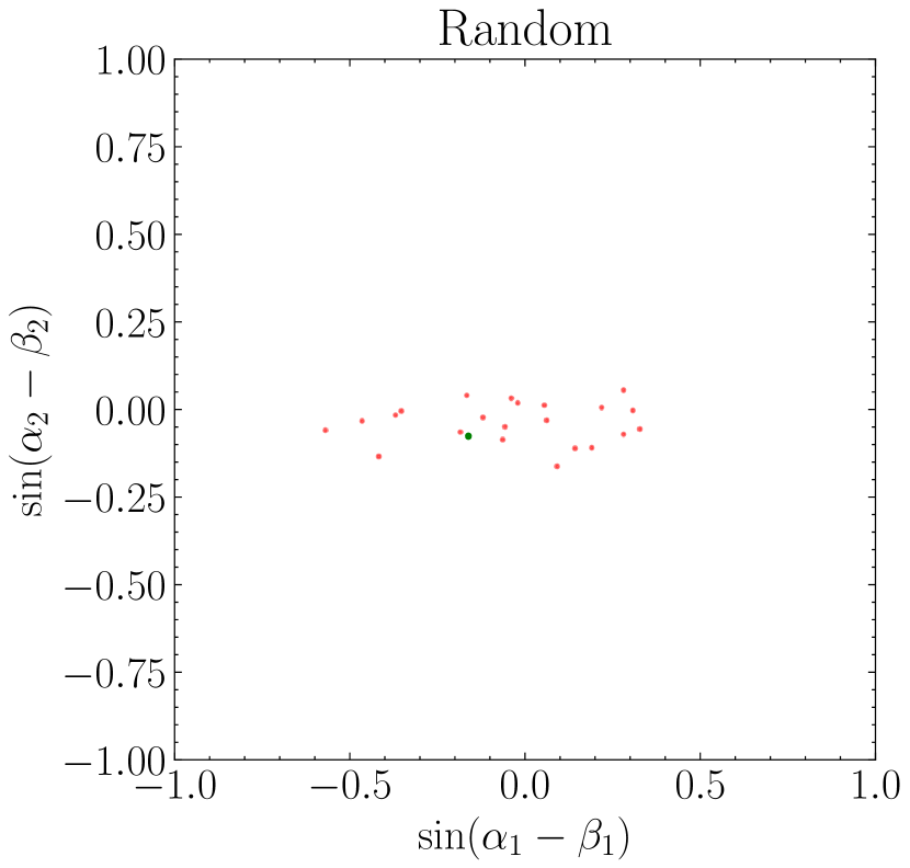
(a) Random sampling

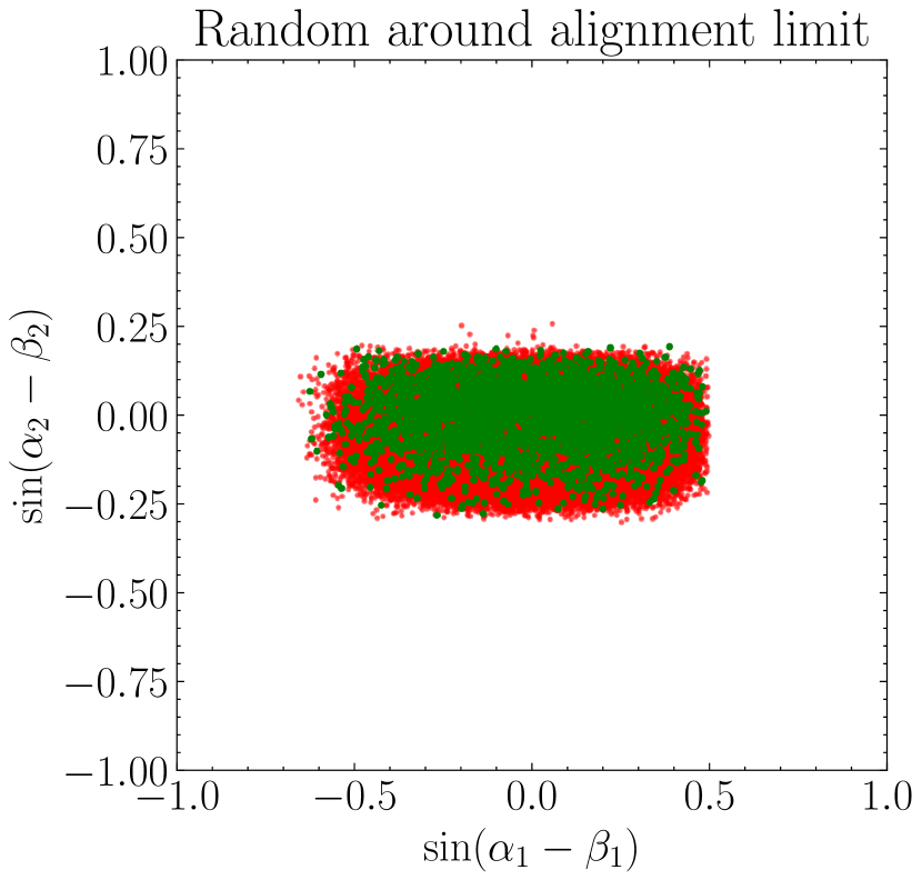
(b) Alignment limit sampling

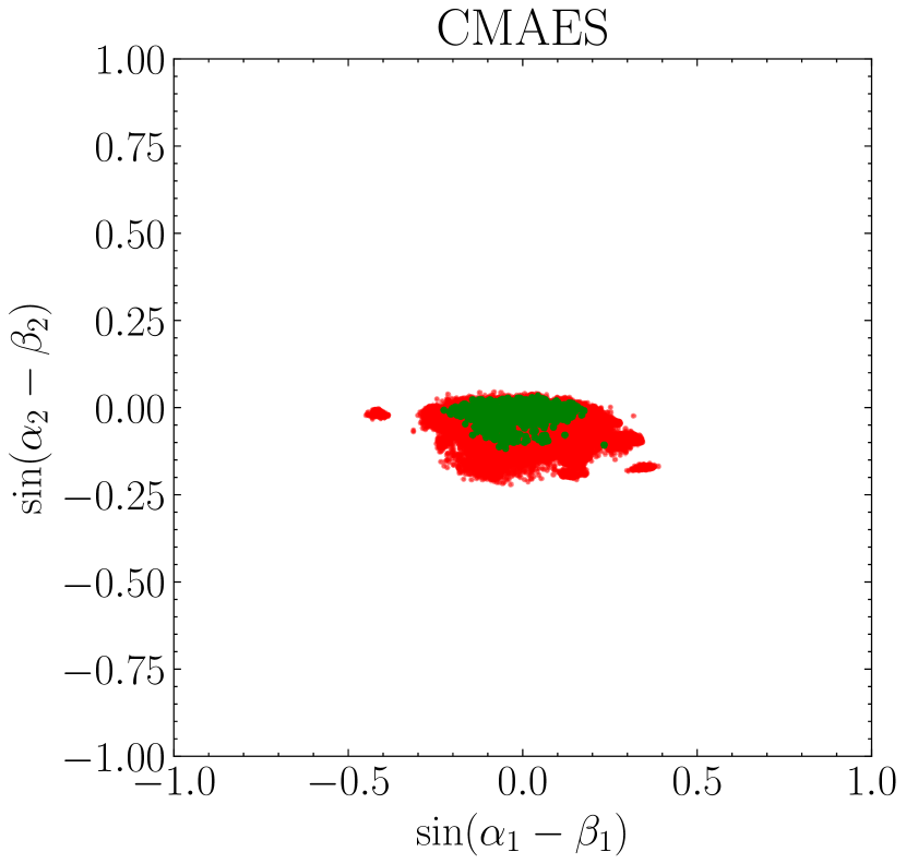
(c) CMAES without exploration

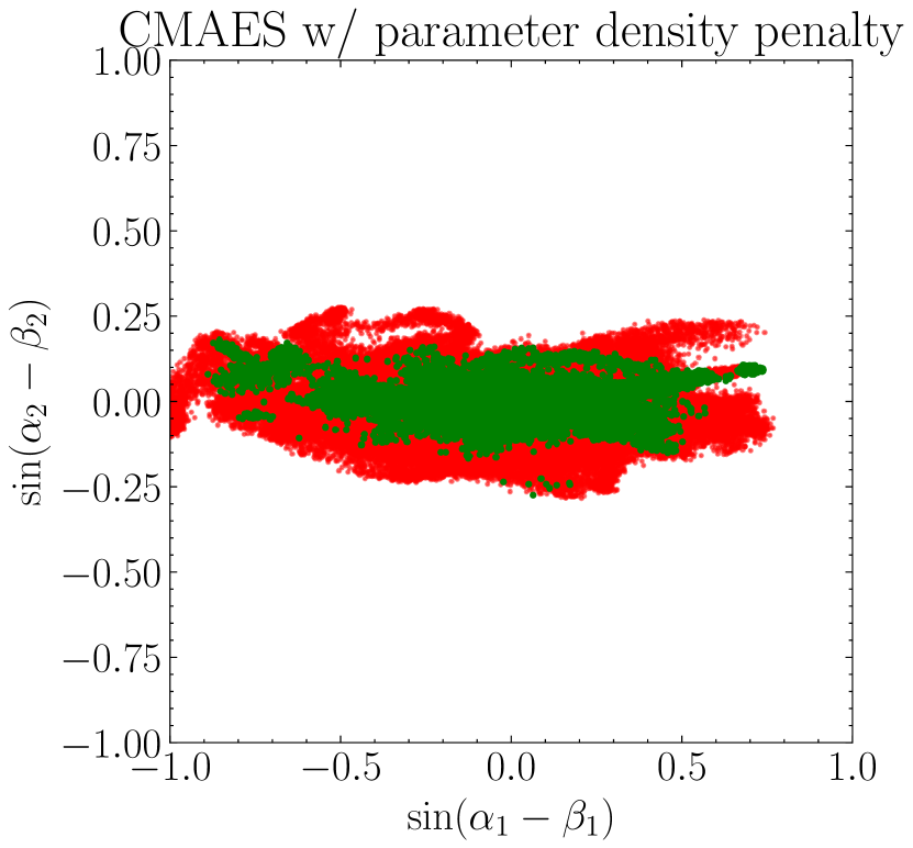
(d) CMAES with parameter novelty reward

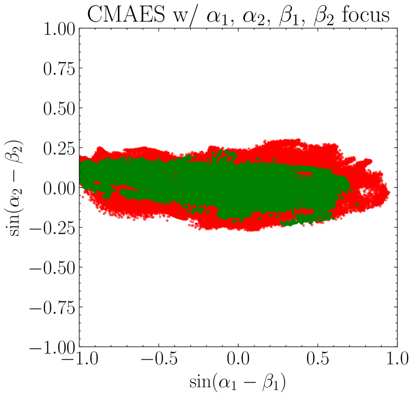
(e) CMAES with parameter novelty reward focused on $(\alpha_{1},\beta_{1},\alpha_{2},\beta_{2})$

Figure 1: $(\sin(\alpha_{1}-\beta_{1}),\sin(\alpha_{2}-\beta_{2}))$ scatter plot for different runs without novelty reward. A point surviving HiggsTools is represented in green, otherwise in red.

Despite the seemingly lacklustre result, the points in fig. 1(c) obtained by CMAES were obtained in a quick run of only around $\mathcal{O}(10^{3})$ attempts, providing around ten orders of magnitude sampling efficiency improvement over the random scan (see section VI.4 for a more detailed discussion on convergence metrics and performance). This allows us to change the sampling logic as to explore the parameter space once the sampler converges into a valid subregion of the parameter space. As explained in the preceding sections, this is achieved by including a parameter density penalty. In fig. 1(d) we show the result for the CMAES runs when activating the novelty reward for all parameters, i.e. using a density penalty for all parameters. We can immediately see a much larger region of the parameter space scanned, especially beyond the alignment limit in the $\sin(\alpha_{1}-\beta_{1})$ direction. We can also observe the first artefact of this methodology: we can see sequences of points, akin to the trail of a paintbrush, in this plane. These trails are in fact the path that CMAES has covered while exploring the parameter space away from previously found points. By introducing the parameter penalty over all parameter space, we were able to find novel points away from the alignment limit. However, because the penalty is computed over all the parameter space, CMAES has no incentive to explore interesting regions of the parameter space, as it can reduce the density penalty by spreading across parameters which have little impact on the constraints. To mitigate this, we focus the parameter density penalty on the four parameters described by these scatter plots, $\alpha_{1},\beta_{1},\alpha_{2},\beta_{2}$. The resulting points can be seen in fig. 1(e), where we see that CMAES was able to spread its exploration even more in the $(\sin(\alpha_{1}-\beta_{1}),\sin(\alpha_{2}-\beta_{2}))$ plane. More interestingly, the points that subsequently pass HiggsBounds, shown in green, cover a much larger region than those obtained using the sampling around the alignment limit, although the latter has arguably a better coverage over $\sin(\alpha_{2}-\beta_{2})$ values more uniformly over different values of $\sin(\alpha_{1}-\beta_{1})$.

The above scans were produced by performing a run without checking for the constraints coming from HiggsBounds provided by HiggsTools. The survival rate against HiggsTools of the points obtained using these scans is $3\%-5\%$, or, in other words, a factor of $1/20$ or less. Furthermore, the execution time with HiggsTools increases by a factor of around $3$. To first approximation, checking for HiggsBounds in the loop can slow down the process of finding good points by an expected factor of $60$ or more. On the other hand, as we can see in fig. 1 not using HiggsTools leads to too many invalid points, and depriving CMAES of this information will only prevent it from finding points that survive HiggsBounds. In fig. 2 we present the first scans with HiggsTools in the loop to check for HiggsBounds constraints. The scans presented in fig. 2(a) and fig. 2(b) are direct analogous to those presented in fig. 1(d) and fig. 1(e), respectively. In both cases we observe a far wider coverage of the parameter space than before, showcasing the importance of providing HiggsTools feedback to CMAES. More importantly, both runs covered the space of valid points around the alignment limit in this plane, but went far beyond in the $\alpha_{1},\beta_{1}$ subspace.

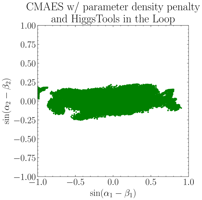
(a) CMAES with parameter novelty reward

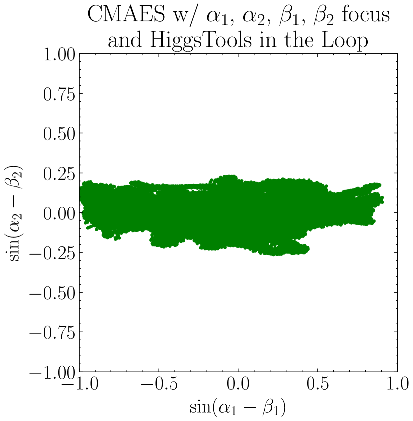
(b) CMAES with parameter novelty reward focused on $(\alpha_{1},\beta_{1},\alpha_{2},\beta_{2})$

Figure 2: $(\sin(\alpha_{1}-\beta_{1}),\sin(\alpha_{2}-\beta_{2}))$ scatter plot for different runs with novelty reward and HiggsTools constraints included in the loss function.

We now turn to the masses of the charged scalars, which are constrained by direct searches. In fig. 3 we show the points obtained in the $(m_{H^{+}_{1}},m_{H^{+}_{2}})$ plane. The logic is similar to the previous discussion, with the difference that the last plot, fig. 3(e), shows the points from a scan where the penalty was focused on the charge scalar masses instead of the mixing angles. From the scan around the alignment limit, fig. 3(b), we can observe how HiggsBounds affects the valid region, especially for small values of scalar masses. Interestingly, in fig. 3(c) we see that CMAES has provided more coverage over this cross section of the parameter space than before. This can be easily interpreted: CMAES works akin to a gradient descent algorithm, but with the performance enhanced by the approximation of local second derivative. This means that CMAES rolls down the loss function with momentum, following the quickest path to its minimum. This preference for a quick convergence path explains why different CMAES runs will provide similar values of the most constrained parameters, as it is through them that a path needs to be found so as to minimise the loss function. This eagerness to converge is a feature of CMAES, which is on the exploitive side of the exploration-exploitation trade off, as previously also discussed [27].

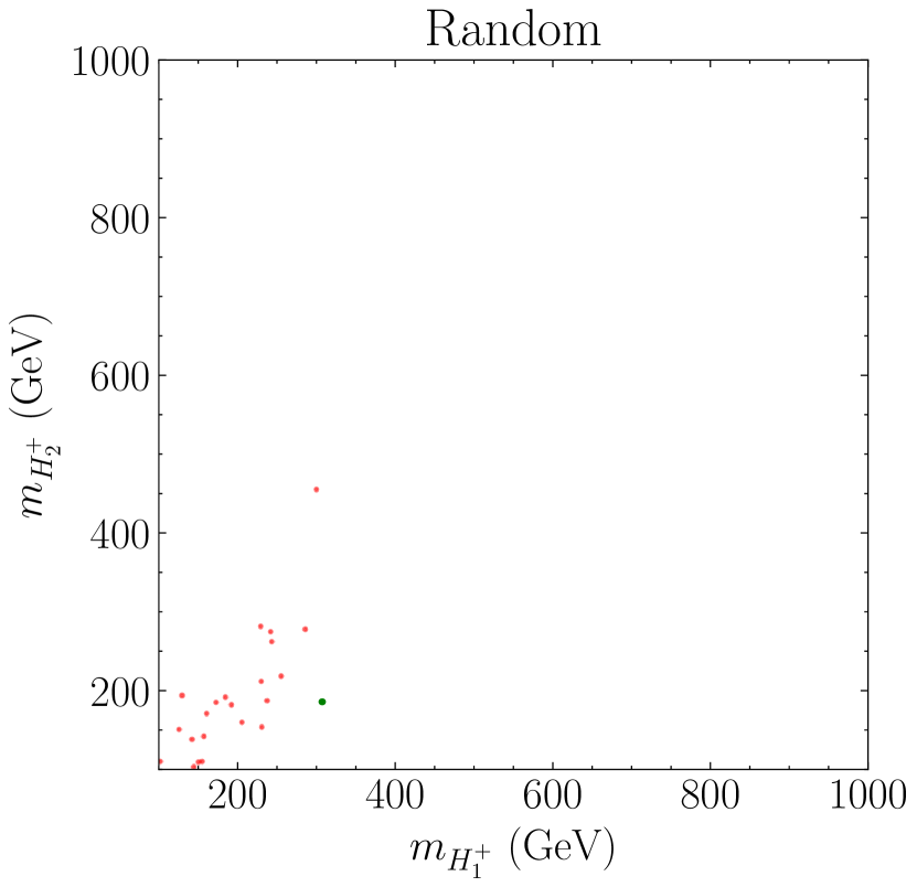
(a) Random sampling

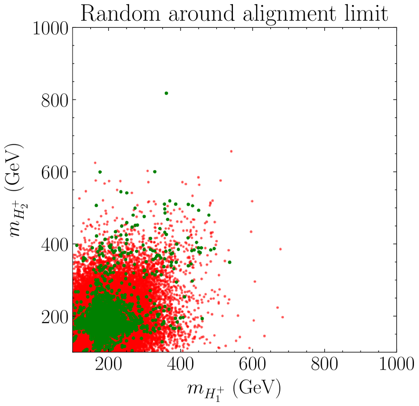
(b) Alignment limit sampling

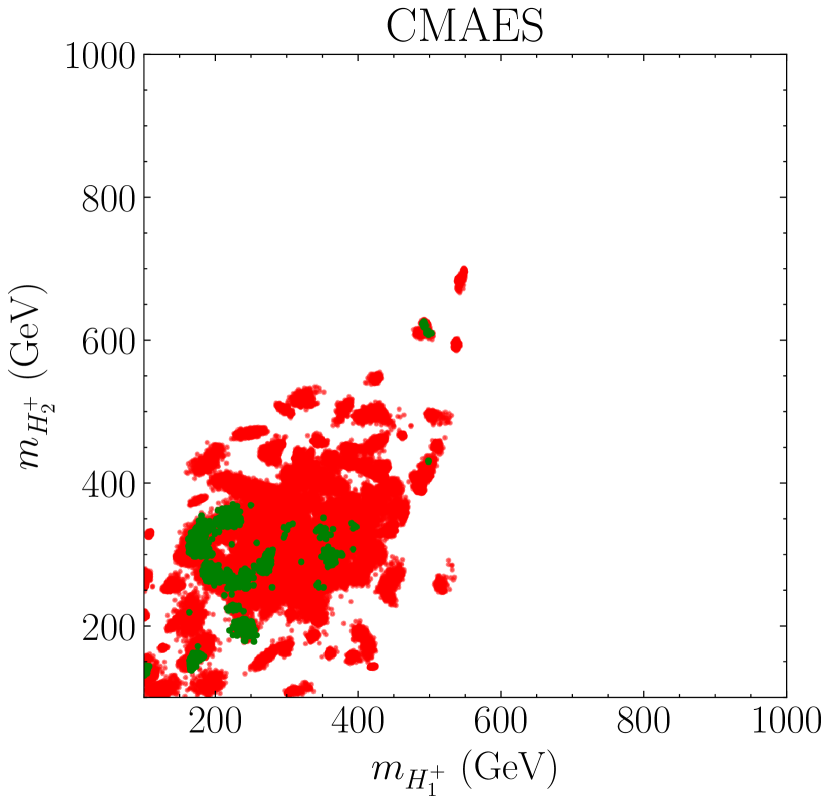
(c) CMAES without exploration

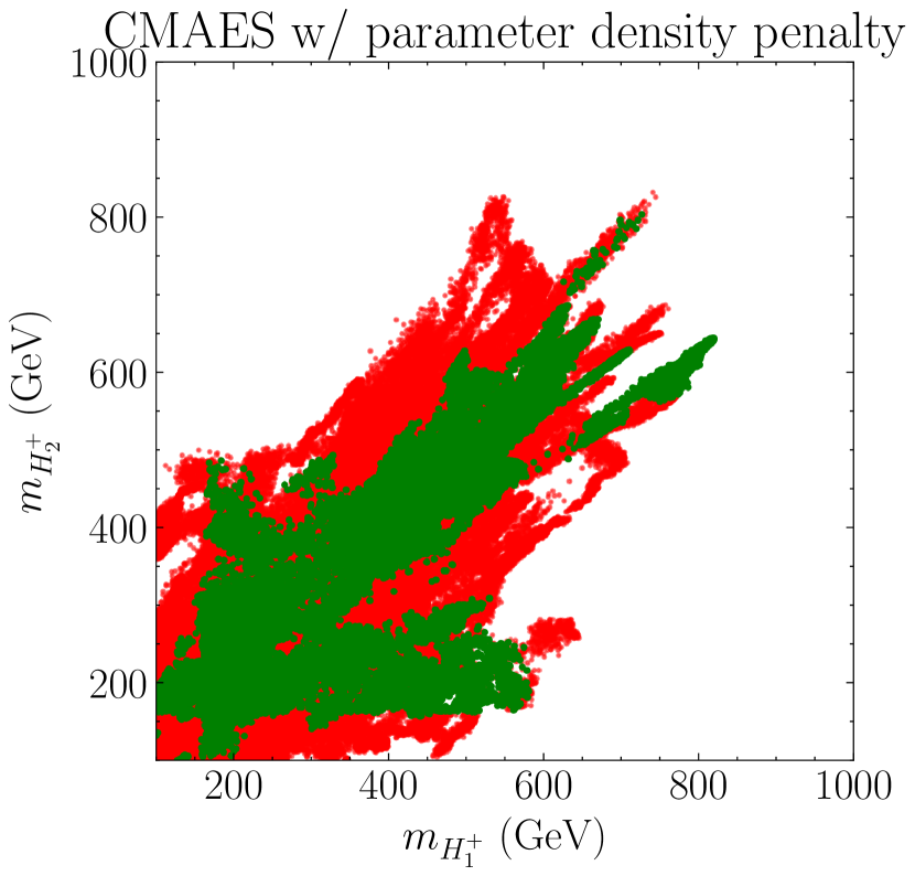
(d) CMAES with parameter novelty reward

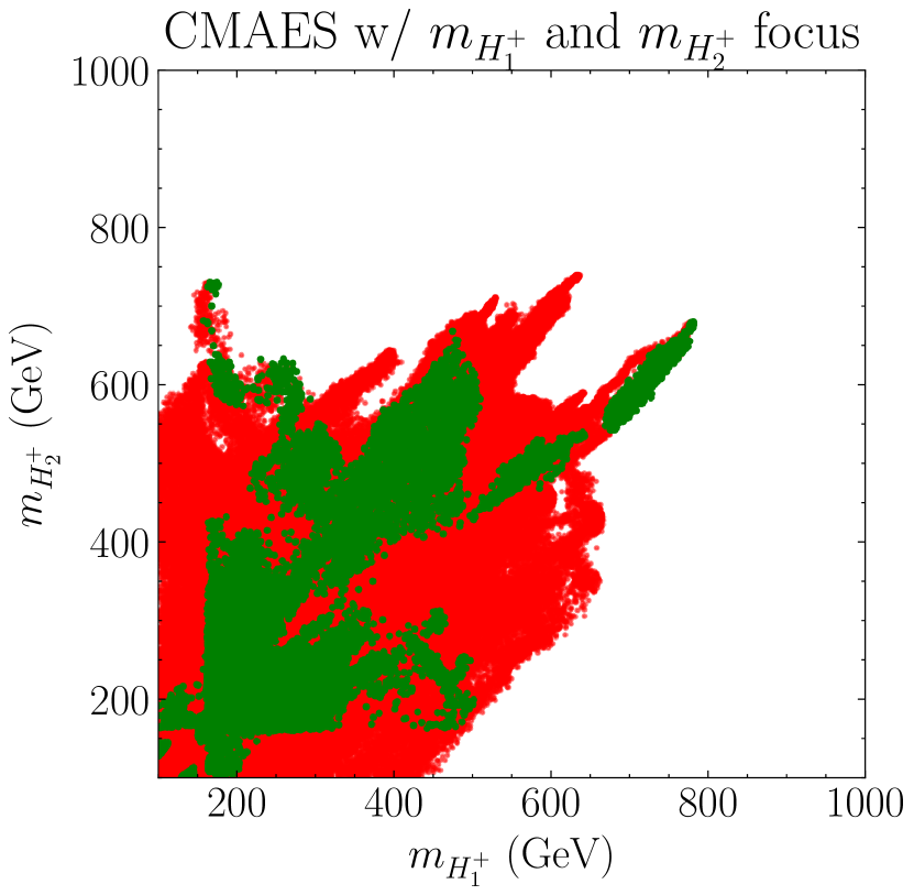
(e) CMAES with parameter novelty reward focused on $(m_{H^{+}_{1}},m_{H^{+}_{2}})$

Figure 3: $(m_{H^{+}_{1}},m_{H^{+}_{2}})$ scatter plot for different runs without novelty reward. A point surviving HiggsTools is represented in green, otherwise in red.

In fig. 3(d) and fig. 3(e) we show the results of the scans with the parameter density penalty over all parameters and focused on the charged masses, respectively. We observe that both were able to cover more parameter space than the alignment limit random scan, but the scan focused on the charged scalar masses was able to cover more of the $(m_{H^{+}_{1}},m_{H^{+}_{2}})$ plane, especially in the $m_{H^{+}_{1/2}}\gtrsim 100$ GeV limits. This result further shows that focussing the exploration reward on subsets of parameters can help uncover novel regions overlooked by traditional scans, although in this case most of the points with $m_{H^{+}_{1/2}}\gtrsim 100$ GeV did not survive HiggsBounds.

Analogously to the discussion above on the mixing angles $\alpha_{1},\ \beta_{1},\ \alpha_{2},\ \beta_{2}$, we now present the results with HiggsTools included in the loop to check HiggsBounds in fig. 4. We see that both with unfocused, fig. 4(a), and charged masses focused, fig. 4(b), novelty reward CMAES is able to cover a much larger parameter space region than the alignment limit sampling. Furthermore, the valid points found also span a larger region than those in fig. 3 that survived HiggsBounds constraints, highlighting the importance of including HiggsTools in the loop.

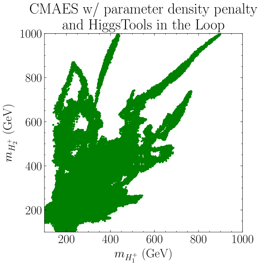
(a) CMAES with parameter novelty reward

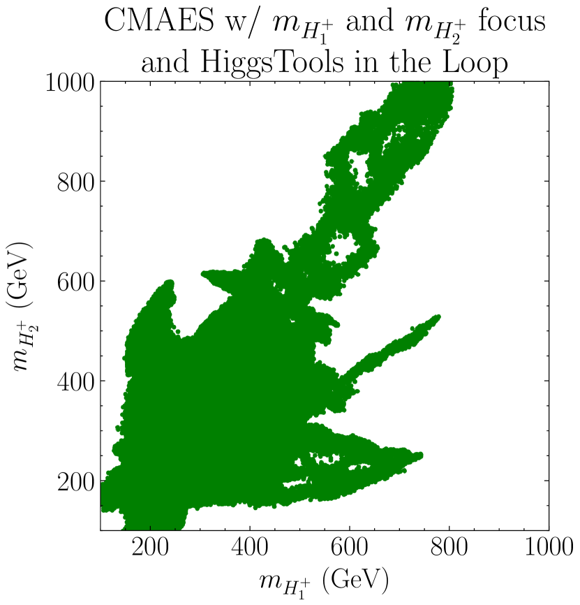
(b) CMAES with parameter novelty reward focused on $(m_{H^{+}_{1}},m_{H^{+}_{2}})$

Figure 4: $(m_{H^{+}_{1}},m_{H^{+}_{2}})$ scatter plot for different runs with novelty reward and HiggsTools constraints included in the loss function.

The paths taken by CMAES while exploring the parameter space are very prominent in the scans just discussed. To better understand how CMAES is exploring, in fig. 5 we show the path traversed by a run projected onto the $(m_{H^{+}_{1}},m_{H^{+}_{2}})$ plane. This run has converged at generation number $129$, with values $(m_{H^{+}_{1}},m_{H^{+}_{2}})\simeq(218.6,151.4)$ GeV. At generation 129, the overall scale of the covariant matrix, given by $\sigma$ of the CMAES algorithm, is $\sigma\simeq 0.002$, a value much smaller than the initialised value of $\sigma=1$. Once converged, the density penalty is then added to the loss function forcing CMAES to explore new values of the parameters, as can be observed in the left pane. As it explores, CMAES might be slowed down by the penalty; this leads the algorithm to increase $\sigma$ to find new good points farther away. On the right pane we see this dynamical adaptation of $\sigma$ by CMAES, with higher (lower) values of $\sigma$ leading to more (less) localised samplings. This ability to adaptively increase $\sigma$ when slowed down also provides CMAES with the capacity to escape local minima, and in our case it provides a way of forcing CMAES to move away from where it has been.

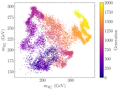
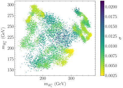
Figure 5: Path of a CMAES scan with focused parameter density penalty on the $(m_{H^{+}_{1}},m_{H^{+}_{2}})$ plane. Left: colour representing the generation number. Right: colour representing $\sigma$, the overall scale of the covariant matrix of CMAES.

VI.1.1 The $m_{H^{+}_{1,2}}\leq 150$ GeV Region

The above results exhibit a peculiar feature that warrants further discussion. Upon closer inspection of the points that survive HiggsBounds when comparing fig. 3 to fig. 4, we see that the scans without HiggsTools in the loop appear to have two islands of points at $m_{H^{+}_{1/2}}\sim 140$ GeV, which the scans with HiggsTools in the loop missed. We present a zoomed look of this region in fig. 6, where we only show the points that have passed HiggsBounds constraints. This suggests that we have not completely mitigated the excessive eagerness of CMAES, which might lead us to miss multimodal solutions, i.e., disjoint valid regions of the parameter space.

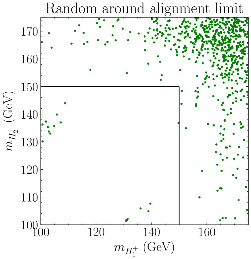
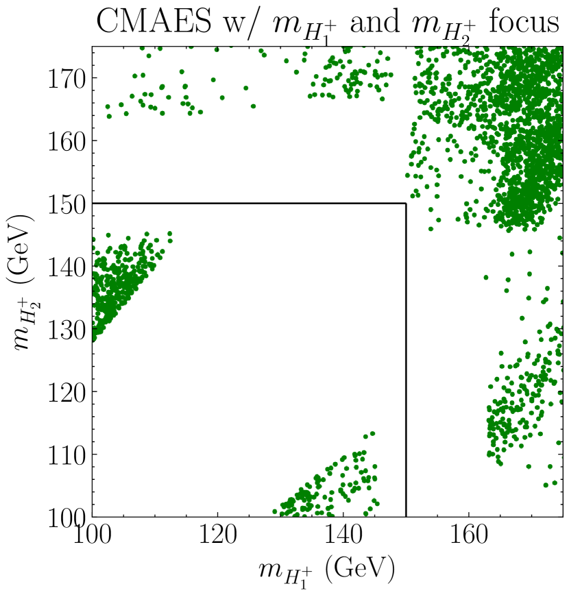
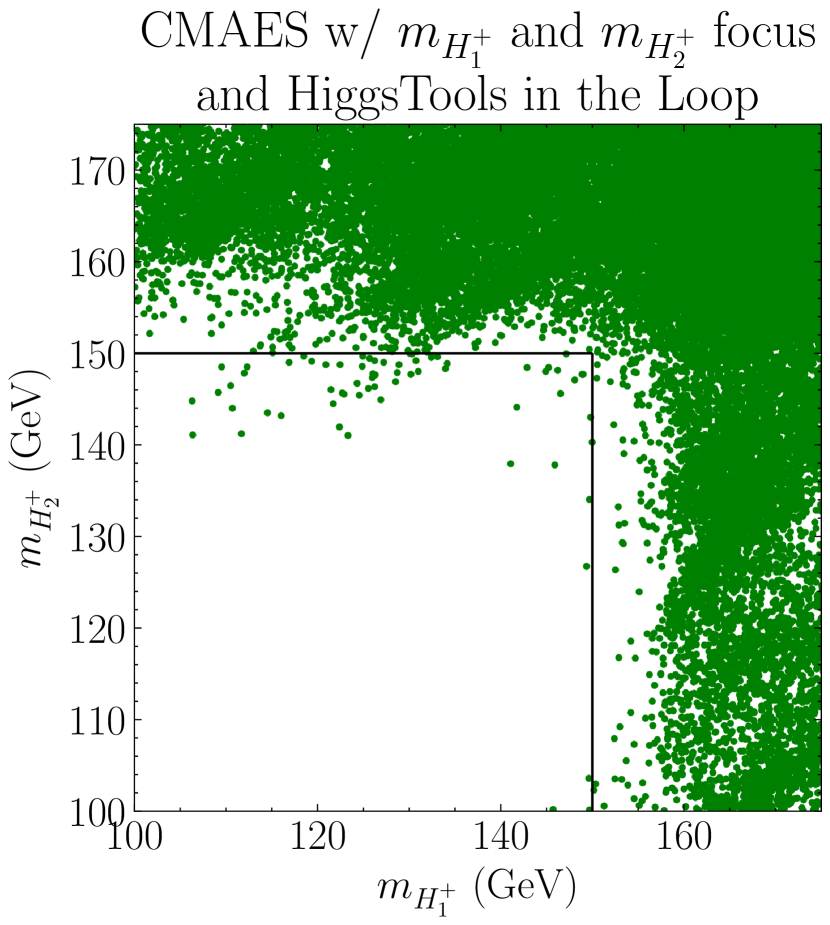
Figure 6: $(m_{H^{+}_{1}},m_{H^{+}_{2}})$ scatter plot zoomed at $m_{H^{+}_{1,2}}\leq 150$ GeV for different runs. Only points passing HiggsBounds constraints are shown.

To better understand whether CMAES is being driven away from this region by its eagerness to converge, we performed a dedicated scan where we restricted the parameter space to $m_{H^{+}_{1,2}}\leq 150$ GeV, and with all other parameter bounds unchanged. We present the result in fig. 7, where we notice that if restricted to that region, CMAES will explore it extensively. Furthermore, we notice that the points $m_{H^{+}_{1/2}}\sim 140$ GeV, which seem above to populate two disjoint regions, do not describe isolated islands of the valid parameter space. There are two important conclusions to draw from this. The first conclusion is that the empty regions of the scatter plot of valid points produced by CMAES do not equate to regions without valid points. This means that one has to be very careful when interpreting these seemingly empty regions without studying them in detail. The second conclusion is that when one focusses on studying these regions, one can find a completely different picture than assumed. In this case the previous results, both from alignment limit scan and from CMAES without HiggsTools in the loop, suggested that there are multiple disjoint regions of valid points in the $(m_{H^{+}_{1}},m_{H^{+}_{2}})$ plane for $m_{H^{+}_{1/2}}\sim 140$ GeV, whereas a closer inspection teaches us that this is not the case.

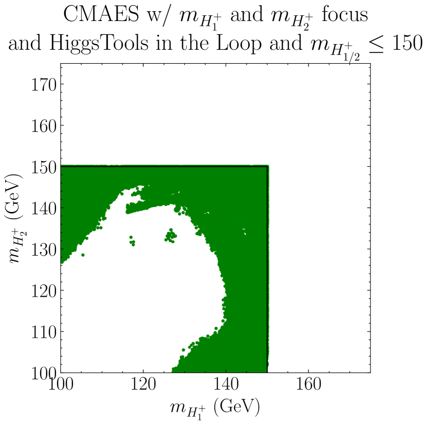
Figure 7: $(m_{H^{+}_{1}},m_{H^{+}_{2}})$ scatter plot for a CMAES run with parameter space restricted to $m_{H^{+}_{1,2}}\leq 150$ GeV.

VI.2 Rewarding Exploration in the Observable Space

So far we have shown how we can improve the parameter space coverage by providing CMAES with a novelty reward in the parameter space by turning on a density penalty in observable values $p(\{\mathcal{O}_{i}\})$. However, a more interesting avenue is to apply the novelty reward to the observable space, $\mathcal{O}$, as this will allow us to assess whether there is new phenomenology obscured by traditional random sampling techniques.

In our first study we want to assess the impact on using a novelty reward in the observable versus the novelty reward in the parameter space studied above. In fig. 8 we show the $(\mu_{ggF,\gamma\gamma},\mu_{ggF,ZZ})$ scatter plots for different scans without HiggsTools in the loop. Similarly to the previous discussions on parameter space coverage, we see that CMAES without further exploration, fig. 8(c), provides a narrower coverage of the observable space than the alignment limit sampling strategy, adding to the intuition that CMAES alone is too eager to converge to be a reliable tool to draw a complete picture of the Physics. This changes considerably once we turn on the parameter space novelty award already studied, which also leads to a greater exploration of the observable space, as can be seen in fig. 8(d). This is easy to interpret, as forcing CMAES to explore the parameter space will always impact the value of the physical quantities of the model. We notice, however, that this is a byproduct of the parameter space exploration, as in this case CMAES does not have an explicit incentive to produce new observable values. In fig. 8(e) we show the result of turning on the density penalty in the observable space, therefore explicitly forcing CMAES to find points with different phenomenology. The result is stunningly different from all the other scans, with CMAES finding points with a far more diverse value than any of the other scans considered so far. Of particular interest, we observe how CMAES can find points with $\mu_{ggF,\gamma\gamma}\simeq 1.2$, which was completely obscured using alignment limit random sampling and painting a very different picture of what phenomenology the $Z_{3}$ 3HDM model can have.

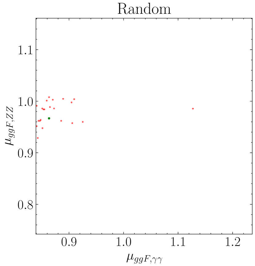
(a) Random sampling

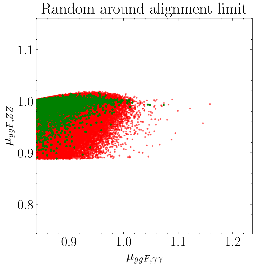
(b) Alignment limit sampling

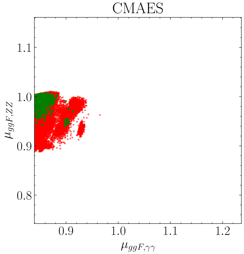
(c) CMAES without exploration

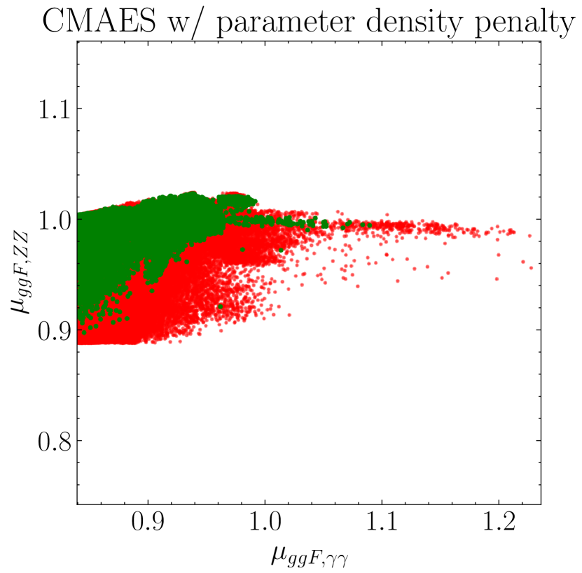
(d) CMAES with parameter novelty reward

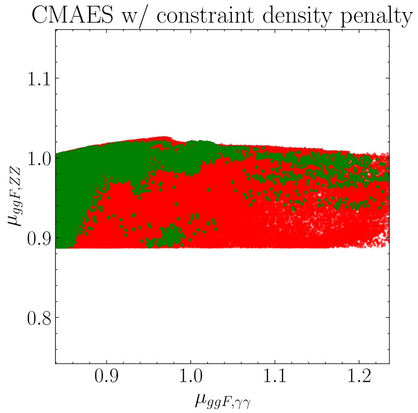
(e) CMAES with observable novelty reward

Figure 8: $(\mu_{ggF,\gamma\gamma},\mu_{ggF,ZZ})$ scatter plot for different runs without novelty reward. A point surviving HiggsTools is represented in green, otherwise in red.

Having shown how an observable space penalty can drive CMAES exploration into novel phenomenological realisations of the model, we now perform the scan with HiggsTools in the loop to endow CMAES with information of the HiggsBounds constraints (themselves added to the loss function and to the penalty). The resulting $(\mu_{ggF,\gamma\gamma},\mu_{ggF,ZZ})$ scatter plot is shown in fig. 9, where we observe how CMAES was able to find points across all allowed values (up to 2-$\sigma$ with experimental measurement) for $\mu_{ggF,\gamma\gamma}$ with $0.89\lesssim\mu_{ggF,ZZ}\lesssim 1.025$, while completely rediscovering the possible values produced by the alignment limit sampling strategy. This result highlights the power and versatility of our methodology to find new phenomenological realisations of a model.

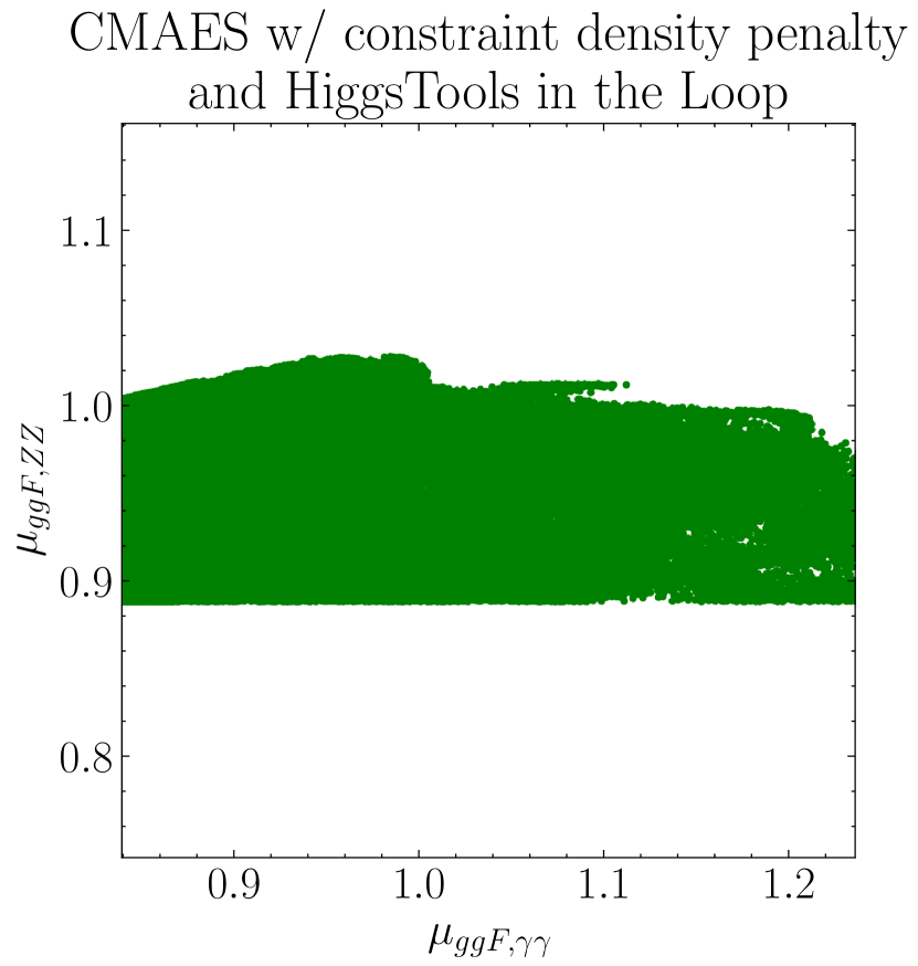
Figure 9: $(\mu_{ggF,\gamma\gamma},\mu_{ggF,ZZ})$ scatter plot for CMAES with novelty reward in observable space and HiggsTools constraints included in the loss function.

Just like we could focus the parameter density on a subset of parameters, we can also focus the observable density penalty on a subset of constraints, allowing one to explore to what extent the model explains certain experimental results. For example, recently [48] ATLAS and CMS have released their most recent measurements of the Higgs decaying to $Z\gamma$ with $\mu_{Z\gamma}=2.2\pm 0.7$, which is just compatible with the Standard Model within 2-$\sigma$. Then one can ask whether the $Z_{3}$ 3HDM model discussed in this work could explain such a high value of $\mu_{Z\gamma}$, considering that, without additional states, the Higgs decay channels are considerably correlated, preventing any particular $\mu_{ij}$ to be large while all others remain small. To study this, we performed a scan with a focused observable density penalty over $(\mu_{ggF,\gamma\gamma},\mu_{ggF,Z\gamma})$, which we present in fig. 10 alongside the scatter plot obtained by the CMAES run with observable density computed over all constraints. Perhaps surprisingly, we see that the scan with the focused density penalty, fig. 10(b), has covered a smaller region than the one with the density penalty computed using all constraints, fig. 10(b). A possible interpretation for this is that the focused density is too constraining, preventing CMAES from finding other ways to populate this plane around other constraints. Conversely, the run with penalty over all constraints will be less demanding for CMAES to explore this subspace, as CMAES will find a way of reducing the penalty by spreading the possible constraint values elsewhere, eventually finding a new route to new values in the $(\mu_{ggF,\gamma\gamma},\mu_{ggF,Z\gamma})$ plane. In other words, although when projected onto the $(\mu_{ggF,\gamma\gamma},\mu_{ggF,Z\gamma})$ plane the valid region appears simply connected, the overall geometry and topology of the valid region of the parameter space are likely far more intricate with focused scans obfuscating these nuances. This interplay between a focused density, the availability of paths for CMAES to explore, and the topological and geometrical details of the valid region is an aspect of our methodology that will be further explored in future work.

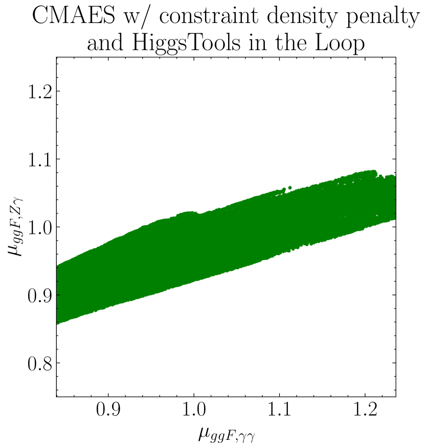
(a) CMAES with observable novelty reward

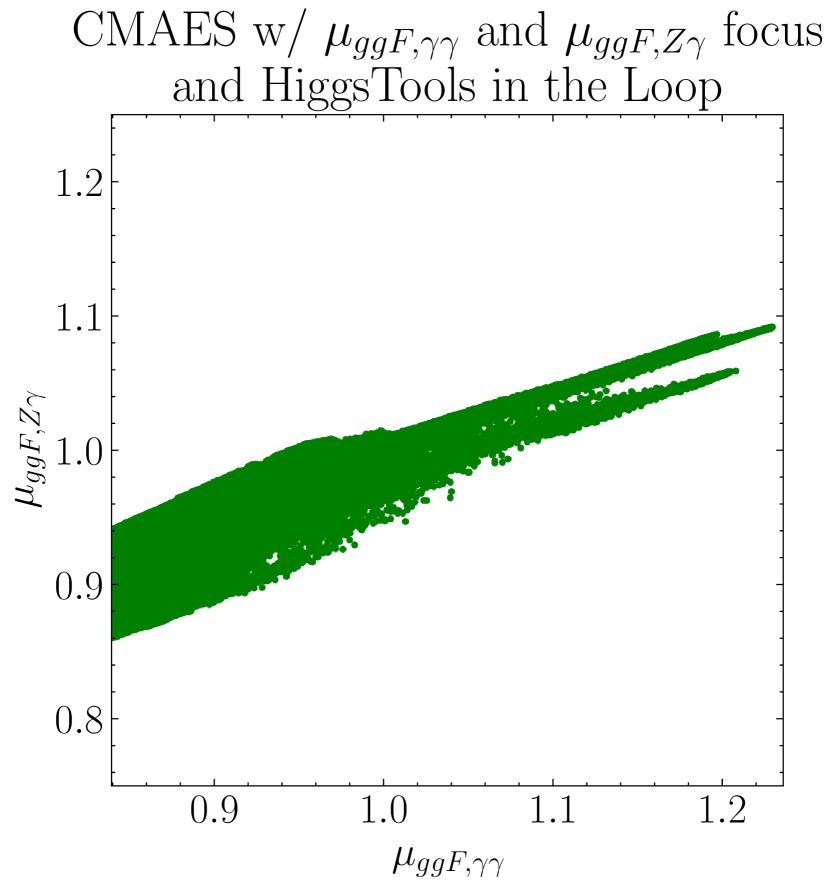
(b) CMAES with observable novelty reward focused on $(\mu_{ggF,\gamma\gamma},\mu_{ggF,ZZ})$

Figure 10: $(\mu_{ggF,\gamma\gamma},\mu_{ggF,Z\gamma})$ scatter plot for CMAES with focused novelty reward in observable space and HiggsTools constraints included in the loss function.

VI.3 Using Points as Seeds for New Runs

The scans performed so far have highlighted the versatility of our methodology in exploring parameter (and observable) spaces. However, the runs performed are independent of each other, i.e., while each run has its own parameter/observable density estimator, this is only trained using valid points found during that run alone.

Then, one can entertain the idea of reusing the information of previous scans to guide new runs in regions of interest. In this section, we explore this idea and provide an example of its implementation by choosing valid points from the previous scans as a seed to new runs. Recalling that CMAES can be initiated with an explicit mean, i.e. starting position, and an overall scale of the covariant matrix, $\sigma$, we can then use a valid point as the starting position of a new scan. In order to start exploring the vicinity of our starting position $\sigma$ cannot be too large, and we found that setting it to $\sigma=0.01$ guarantees that CMAES starts already at the minimum of the constraint loss function.

Seed points were identified by running HBOS on the entire collection of valid points (left pane of fig. 11). For this concrete example, we evaluated the density only on the $(m_{H^{+}_{1}},m_{H^{+}_{2}})$ subspace and identified the $1\%$ outliers (middle pane of fig. 11), i.e., the points representing the least explored parts of the valid region of the parameter space. We notice some of the shortcomings of HBOS as the density estimator in this plot: given that HBOS fits a histogram to each dimension to compute the density, a point might be in a relatively sparse region but might not be picked as an outlier if one of its components is in a populated bin. For example, we see that the outliers are not necessarily at the rim (convex haul) of the space, but in regions where there are few points both in $m_{H^{+}_{1}}$ and $m_{H^{+}_{2}}$. This same shortcoming of HBOS is present in the scans with novelty reward, leaving room for improvement to be explored in future work.

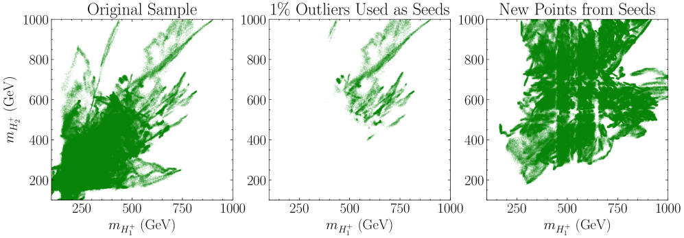
Figure 11: $(m_{H^{+}_{1}},m_{H^{+}_{2}})$ scatter plot for the seeded run. Left: The whole collection of valid points obtained by the other scans. Middle: The $1\%$ outliers classified by HBOS. Right: New points obtained by the seeded runs started at points randomly selected from the $1\%$ outliers.

With the most outlying valid points identified, we ran $100$ scans not only seeded by a point randomly chosen from the $1\%$ outlier subset, but with the density penalty also making use of the outliers to guide the new scans away from the already explored regions. We did not use the whole sample of valid points to train the density estimator as it is comprised of over 4 million valid points, considerably slowing down the scan. In the right pane of fig. 11 we show the resulting valid points found by the seeded scans, where we observe that CMAES was able to explore even further away from the previously chartered valid region. Clearly, one could now use the new points as new seeds in repeated iterations to explore even more this subsection of the parameter space, or any other section of it or of the observable space, in order to draw an even more global picture of the valid region. The caveat of only using chained scans is that one can only explore regions that are simply connected to the seed, a detail which must be kept in mind when employing this strategy. Finally, we notice that the scatter plot appears to have some vertical and horizontal regions with less points, this is an artefact of HBOS which draws a histogram with $100\times 100$ bins in this subspace, impacting the density value along horizontal and vertical strips with width similar to the width of the bins.

VI.4 Convergence Metrics

Having discussed how density penalties can be used to enhance the CMAES exploration of the parameter space, we now turn to another aspect of our methodology: the convergence speed. Recalling that CMAES operates by minimising the total loss function, $L_{T}$ from eq. 31, we show how its value decreases sharply after just a few generations in fig. 12, where we also provide the values of random generations for comparison. More precisely, after just 100 generations, totalling around just 1200 points, CMAES has nearly converged to the valid region of the parameter space.

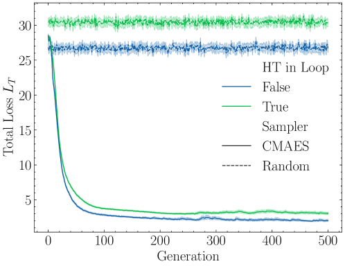
Figure 12: Total loss as function of generation. Only the first 500 generations are shown. The random sampler curves are over random generations of $12$ poitns, the same population size as CMAES. The shaded regions represent $0.95$ confidence intervals computed using a bootstrap of 100 runs.

Despite the suggestive previous plot, not all scans converge within the budget, which we set to 100 runs of 2000 generations for each case in table 1 without HiggsTools, and to 200 runs of 2000 generations for the cases with HiggsTools. We present these metrics in table 2 alongside statistics on the fraction of valid points that are within the alignment cases, AL-1 from eq. 26 and AL-2 from eq. 27. We see that, while most points are within AL-1, only a minority are within AL-2. More interestingly, we observe how the scan with novelty reward in the $\alpha_{1},\ \beta_{1},\ \alpha_{2},\ \beta_{2}$ subspace of the parameter space has produced the most points away from the alignment limit. This can be visually understood in fig. 1 and fig. 2 where it is clear that the novelty reward is guiding CMAES to values of $\alpha_{1},\ \beta_{1}$ that are beyond the alignment limit bounds. This is a feature of the versatility of our methodology, as we can perform dedicated scans explicitly away from previously considered priors and regions of the parameter space.

Sampling Scan Converged Runs Within AL-1 Within AL-2 CMAES No penalty (Vanilla) 97 out of 100 $1.00$ $1.5\times 10^{-2}$ Parameter space penalty 95 out of 100 $0.90$ $5.1\times 10^{-3}$ Constraint space penalty 90 out of 100 $0.99$ $1.8\times 10^{-4}$ $\alpha_{1}$, $\beta_{1}$, $\alpha_{2}$, $\beta_{2}$ focus 94 out of 100 $0.85$ $5.9\times 10^{-3}$ $\mu_{ggF,\gamma\gamma}$ and $\mu_{ggF,Z\gamma}$ focus 91 out of 100 $1.00$ $4.2\times 10^{-5}$ $m_{H_{1}^{+}}$ and $m_{H_{2}^{+}}$ 90 out of 100 $0.95$ $6.6\times 10^{-3}$ CMAES Parameter space penalty 92 out of 200 $0.92$ $1.1\times 10^{-2}$ w/ HT Constraint space penalty 111 out of 200 $0.94$ $1.4\times 10^{-2}$ $\alpha_{1}$, $\beta_{1}$, $\alpha_{2}$, $\beta_{2}$ focus 102 out of 200 $0.84$ $4.1\times 10^{-2}$ $\mu_{ggF,\gamma\gamma}$ and $\mu_{ggF,Z\gamma}$ focus 101 out of 200 $0.93$ $4.1\times 10^{-3}$ $m_{H_{1}^{+}}$ and $m_{H_{2}^{+}}$ 91 out of 200 $0.98$ $5.3\times 10^{-2}$

Table 2: Convergence and coverage statistics of the different scans presented in table 1. While the first CMAES rows correspond to scans without HiggsTools in the loop, the corresponding fractions of points in both alignment cases are computed using points that have passed HiggsBounds constraints after the scan.

As CMAES converges, it will start to find good points. This can be seen in fig. 13 where we observe that after around 100 generations for the runs without HiggsTools in the loop, and after around 200 generations for the runs with HiggsTools in the loop, CMAES starts finding valid points.

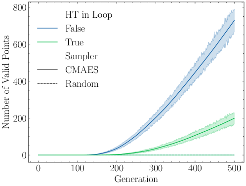
Figure 13: Number of valid points founds as function of generation. Only the first 500 generations are shown. The random sampler curves are over random generations of $12$ points, the same population size as CMAES. The shaded regions represent $0.95$ confidence intervals computed using a bootstrap of 100 runs.

Before HT After HT Points Efficiency Points Efficiency AL-1 21 in $4.4\times 10^{12}$ $\mathcal{O}(10^{-11})$ 0 in $4.4\times 10^{12}$ $<\mathcal{O}(10^{-12})$ AL-2 13 701 in $10^{10}$ $\mathcal{O}(10^{-6})$ 510 in $\times 10^{10}$ $\mathcal{O}(10^{-8})$ Random 23 in $10^{13}$ $\mathcal{O}(10^{-12})$ 1 in $10^{13}$ $\mathcal{O}(10^{-13})$

Table 3: Sampling efficiencies of random sampling strategies. We note that for the completely random scan the numbers are estimated.

In fig. 14 we show the distribution of the generation where the first valid point was valid for the runs with and without HiggsTools in the loop. We see that checking for HiggsBounds postpones the discovery of the first good point by a factor of around $2$ in terms of generation number. However, this is far better than with random sampling (both purely random and around the alignment limit) where only at most $5\%$ of the points that respect all other constraints survive HiggsBounds constraints, table 3. Additionally, we note that the number of trial points needed to find a good valid point is around $\mathcal{O}(250-750)\times 12$ when not including HiggsBounds constraints in the loop, and $\mathcal{O}(400-1300)\times 12$ when including HiggsBounds constraints in the loop. Recall that the efficient sampling of the random sampler is (estimated) to be $\mathcal{O}(10^{-12})$ and $\mathcal{O}(10^{-13})$ respectively, which means that our methodology improves the sampling efficiency by a factor of 8 orders of magnitude, even if we do not consider the near perfect sampling efficiency after convergence during the density penalty-guided exploration phase. Unsurprisingly, the improvement over the AL-2 alignment limit sampling strategy is more modest, with around four orders of magnitude when considering HiggsBounds constraints, but we reiterate that this only pertains to the first convergence and that our algorithm can then continue to explore the region found and go beyond the alignment limit bounds, as was highlighted in the previous section.

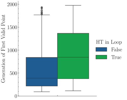
Figure 14: Distribution of the generation with the first valid point. The distributions shown are obtained from all runs with and without HiggsTools in the loop.

So far, we have seen the improvements to convergence provided by CMAES by taking into account the number of points tried, observing massive improvements over random sampling. On the other hand, the methodology presented in this work is only useful if it also provides a speed-up in terms of wall time, i.e. time passed from the reference frame of the user. In fig. 15 we present a variation of fig. 14 but in terms of elapsed time, instead of generations. We see that CMAES without including HiggsBounds constraints in the loop tends to find points within $\mathcal{O}(100-500)$ seconds, i.e. in minutes, while when including HiggsBounds constraints, this increases do $\mathcal{O}(750-2250)$ seconds. The slowing down is easily understood: using HiggsTools slows down the evaluation of a point by a factor of around 3 (see below for more details), and since converging on HiggsBounds constraints delays CMAES in finding a good point by a factor of around 2 (see discussion above) we expect an overall wall time delay of 5, which is what we can see here.

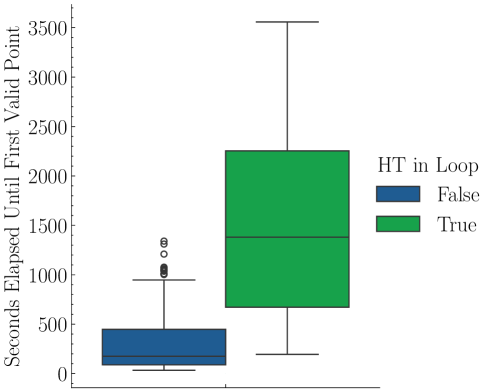
Figure 15: Distribution of the elapsed time until the first valid point. The distributions shown are obtained from all runs with and without HiggsTools in the loop.

To better understand the impact of the different components of our methodology in the total time, we present in table 4 the times taken by different steps of the loop for CMAES and the random sampler, and with and without HiggsTools in the loop. In this table, generation time represents the time needed to perform all the steps of a generation including evaluation time, i.e. the time needed to compute all observables (including HiggsBounds, when applicable), train the density estimator (when applicable), and perform diverse housekeeping tasks such as save intermediate results, keep track of run metrics, etc. In this table we see that the overall housekeeping overhead can be assessed in the random sampler rows as for these there is no overhead related to CMAES and to density estimation, and it is around 0.015 (0.019) seconds without (with) HiggsTools. The most important observation to take from this table is that the overall overheard of our methodology, including that associated with CMAES and density estimation, is at most around $10\%$ of the total generation time for the CMAES runs without HiggsTools. Once we include HiggsTools in the loop, the overall generation time increases 3-fold but the overhead remains mostly the same, showing that our methodology provides even greater gains for problems with a slow evaluation time. Additionally, we see that our choice of HBOS for density estimator corresponds to a minor fraction of the overhead. However, one can notice that the standard deviation of the density estimator training is greater than the mean; this is because HBOS has a linear computational complexity with respect to the number of valid points, effectively becoming slower to train the more valid points we have found. Improvements to the density estimator are left for future work.

Sampler HT in Loop Generation Evaluation Density Estimator Overhead (sec) (sec) Training (sec) (sec) CMAES False $0.48\pm 0.16$ $0.43\pm 0.15$ $(3.9\pm 23)\times 10^{-3}$ $0.055\pm 0.043$ True $1.6\pm 0.3$ $1.6\pm 0.2$ $(1.9\pm 22)\times 10^{-3}$ $0.068\pm 0.048$ Random False $0.33\pm 0.06$ $0.31\pm 0.06$ N/A $0.015\pm 0.003$ True $1.4\pm 0.2$ $1.3\pm 0.2$ N/A $0.019\pm 0.012$

Table 4: Comparison of times taken by different parts of the loop for CMAES and random sampler with and without HiggsTools in the loop. The times refer to a generation of 12 points in every case. The values presented are the mean $\pm$ one standard deviation over the scans falling in each of the four categories.

VII Conclusions

In this paper, we have developed a novel approach to explore the highly constrained multidimensional parameter space of the $Z_{3}$ 3HDM, defined in section II and constrained discussed in section III and appendix A, and go beyond alignment limit priors presented in section IV, by combining CMAES power of exploration with a Machine Learning estimator for point density.

It is important to note that, while the subject of study in this paper was the $Z_{3}$ 3HDM parameter space, our approach is general and applicable to any Physics case, providing a solution to the difficulty of sampling good points in highly constrained multidimensional parameter spaces.

In section V we introduced our strategy, using CMAES, a powerful evolutionary strategy, in combination with HBOS, a fast ML model for density estimation. Our approach guarantees that the density-based novelty reward does not compete in the loss function with the constraints on the model and pushes CMAES to explore the parameter space once converged. Importantly, we showed how our methodology is versatile, as we can turn on the novelty reward in the parameter space or in the observable space, where the phenomenology is realised. Additionally, the novelty reward can be computed by estimating the density in only a subset of parameters and/or observables, allowing for quick focused scans on regions of interest.

In section VI we presented the results of multiple scans performed with our methodology, each with different combinations of parameters and/or observables on which the density penalty was computed. We showed how our approach can effortlessly go beyond the alignment limit sampling strategies, finding valid points in regions of the parameter space hitherto ignored by such sampling strategies. More precisely, using the novelty reward in the parameter space, both in whole or in a subset, in section VI.1 we have found that it is easy to go beyond the alignment limit in the $(\alpha_{1},\beta_{1})$ plane. In the same analysis, we showed how our methodology also exposes regions of heavy scalar masses, even preferring it over the region excluded by HiggsBounds, which we explored in detail in section VI.1.1 by restricting the parameter space to $m_{H^{+}_{1,2}}\leq 150$ GeV, finding a considerably different picture of that region of the parameter space that one would get from alignment limit sampling.

While we set ourselves to explore the parameter space with CMAES combined with a novelty reward, the Physics of the model resides its space of observables and physical quantities. In section VI.2 we have the results of scans where the density penalty was computed in the observable space instead of the parameter space. The results uncover novel possible phenomenological realisations of the 3HDM, an important contribution of this work that would not have been possible to achieve without our AI-based scan. In particular, we find that it is possible to accommodate Higgs decay signal strengths larger than one up to their current upper experimental bounds, a phenomenological signature not captured by alignment limit random sampling strategies. Given the versatility in exploring different observables, we set to study whether the $Z_{3}$ 3HDM can explain the recent measurement of $\mu_{Z\gamma}\simeq 2.2$ by ATLAS and CMS [48], finding that $\mu_{Z\gamma}\lesssim 1.1$ in the $Z_{3}$ 3HDM, not a surprising result given that decay signal strengths are highly correlated in this model and one cannot get arbitrarily high values for one of them without spoiling the experimental measurements of the remainder (for other possibilities, see, for instance, the discussion in [49]). Finally, in section VI.4 we discuss the convergence metrics of our algorithm and compare it with the pure and alignment limit random sample strategies. Our methodology is orders of magnitude faster (both in number of tried points and wall time) than the random sampling strategies, providing a solution to the random sampling efficiency problem in highly constrained multidimensional parameter spaces.

Although the methodology presented in this work provides impressive speedup and efficiency improvement when compared to random sampling strategies, we have encountered some shortcomings and less appealing characteristics that we want to improve in future work. First, the methodology used in the analyses employs independent runs, each with its own density estimator from which the novelty reward is derived. An alternative approach is to share information across runs to ensure the novelty of the exploration. In section VI.3 we showed how such a strategy could be implemented, where we identified the valid region of the parameter space less populated (in the $(m_{H^{+}_{1}},m_{H^{+}_{2}})$ subspace) by our scans and then used some of the points in that region as a seed for new runs. The resulting new points were significantly different from the ones found previously, highlighting the potential for even further exploration by chaining runs together, a methodological detail that can be improved in the future. Second, in the same study, we encountered some artefacts arising from the binning nature of the HBOS, which can, in principle, be mitigated by using a different density estimator (or a different novelty detector). In our early exploration, we tried a variety of alternatives, all significantly slower than HBOS, making our methodology impractical. Producing a better way of assigning the novelty reward could solve the binning problem and any manifestation of the curse of dimensionality produced by it. Third, we have observed that our methodology might not explore all possible regions as CMAES intuitively follows a path of fastest descent. This was particularly clear in section VI.1.1 where we addressed the overlooked region of small charged scalar masses. By restricting the parameter space, we were able to populate that region easily, but the fact that it was not explored in the first place shows that we need to be careful when interpreting empty regions as regions without valid points. Lastly, we have observed that the geometrical and topological details of the valid region of the parameter space might impact the possible exploration paths of CMAES. This can have a profound effect on the results when there are disjoint, not simply connected, regions of the parameter space supporting good points. We leave to future work the development of a way to assess whether the scans are capable of capturing multimodal valid regions confidently.

Finally, our methodology opens up the possibility for a complete exploration of other $N$HDM (or any other BSM Physics) parameter spaces in light of the current highly constraining experimental results and theoretical conditions. As our work shows, this could lead to novel phenomenological realisations of these models and, ultimately, to the possibility of novel experimental signatures. We leave this phenomenological study for the future.

Appendix A Description of the various constraints

In this appendix, we summarise the constraints that have to be satisfied for a point in parameter space to be considered a valid point. As these have already been discussed in great detail in a series of papers [10, 12, 16], here we just give a brief review and indicate the places where to look for further information. We list the constraints in the order in which they are applied in the code.

A.1 The $\kappa$’s formalism

We found that it is useful to select points that are already close to the LHC constraints, using the $\kappa$’s formalism. We require them to be within 3$\sigma$ of the LHC data [50]. The expressions for the $\kappa$’s for the different types of fermion couplings in the 3HDM are given in [12]. As in this work we just consider Type I, we have for the fermions,

$$\kappa_{U}=\frac{\sin(\alpha_{2})}{\sin(\beta_{2})},\quad\kappa_{D}=\frac{\sin(\alpha_{2})}{\sin(\beta_{2})},\quad\kappa_{L}=\frac{\sin(\alpha_{2})}{\sin(\beta_{2})}.$$ (35)

The couplings with the vector bosons give, for all types,

$$\kappa_{W}=\cos(\alpha_{2})\cos(\alpha_{1}-\beta_{1})\cos(\beta_{2})+\sin(\alpha_{2})\sin(\beta_{2})\,,$$ (36)

which gives $\kappa_{W}=1$ when $\alpha_{1}=\beta_{1}$ and $\alpha_{2}=\beta_{2}$. We should note that the points are subsequently tested for the signal strengths, so this constraint is applied with a large interval (3$\sigma$) just to make the selection faster.

A.2 Bounded From Below (BFB)

The scalar potential has to be BFB. As explained in ref.[12], to find the necessary and sufficient conditions for this to happen is a difficult task. For the 3HDM is only known for a few cases with high symmetry in the potential. For the $Z_{3}$ 3HDM that we consider here, the best we can do is to use sufficient conditions. We refer to ref.[12] for the details of the implementation.

A.3 Oblique parameters $S,T,U$

To discuss the effect of the electroweak precision parameter, S, T and U, we use the expressions in [33] and the experimental summary in [34, 51]. The expression for the needed matrices $V$ ($3\times 6$) and $U$ ($3\times 3$) is [12],

$$V=\begin{pmatrix}i\textbf{P}^{T}_{11}&\textbf{R}^{T}_{11}&\textbf{R}^{T}_{12}&\textbf{R}^{T}_{13}&i\textbf{P}^{T}_{12}&i\textbf{P}^{T}_{13}\\ i\textbf{P}^{T}_{21}&\textbf{R}^{T}_{21}&\textbf{R}^{T}_{22}&\textbf{R}^{T}_{23}&i\textbf{P}^{T}_{22}&i\textbf{P}^{T}_{23}\\ i\textbf{P}^{T}_{31}&\textbf{R}^{T}_{31}&\textbf{R}^{T}_{32}&\textbf{R}^{T}_{33}&i\textbf{P}^{T}_{32}&i\textbf{P}^{T}_{33}\end{pmatrix},$$ (37)

and

$$U=\textbf{Q}^{T},$$ (38)

where the matrices $\textbf{R},\textbf{P},\textbf{Q}$ were defined before.

A.4 Unitarity

A valid point in the parameter space must also satisfy the perturbative unitarity constraints. This can be expressed in terms of constraints on the $\lambda_{i}$ potential parameters. For the different symmetry constrained 3HDM these are fully given in [11] to which we refer the reader for further details.

A.5 The signal strengths $\mu_{ij}$

The LHC results on the 125 GeV Higgs boson are normally given by the signal strengths,

$$\mu_{if}=\left(\frac{\sigma_{i}^{\text{3HDM}}(pp\to h)}{\sigma_{i}^{\text{SM}}(pp\to h)}\right)\left(\frac{\text{BR}^{\text{3HDM}}(h\to f)}{\text{BR}^{\text{SM}}(h\to f)}\right)\,,$$ (39)

where the subscript ‘$i$’ denotes the production mode and the subscript ‘$f$’ denotes the decay channel of the SM-like Higgs scalar. The relevant production mechanisms include gluon fusion ($ggF$), vector boson fusion ($VBF$), associated production with a vector boson ($VH$, $V=W$ or $Z$), and associated production with a pair of top quarks ($ttH$). The SM cross section for the gluon fusion process is calculated using HIGLU [52], and for the other production mechanisms we use the prescription of Ref. [53]. The calculated $\mu_{if}$ are required to be within 2$\sigma$ of the LHC results[32].

A.6 Constraints from flavour data

In Type-I, by construction, 3HDM there are no FCNCs at the tree-level. Therefore, the only NP contribution at one-loop order to observables such as $b\to s\gamma$ and the neutral meson mass differences will come from the charged scalar Yukawa couplings. We follow [9] where it was shown that the constraints coming from the meson mass differences tend to exclude very low values of $\tan\beta_{1,2}$. Therefore, we only consider

$$\tan\beta_{1,2}>0.3\,,$$ (40)

to safeguard ourselves from the constraints coming from the neutral meson mass differences.

To deal with the constraints resulting from $b\to s\gamma$, we follow the procedure described in Refs. [39, 10, 54] and impose the following restriction

$$2.87\times 10^{-4}<\text{BR}(B\to X_{s}\gamma)<3.77\times 10^{-4}\,,$$ (41)

which represents the $3\sigma$ experimental limit. As in the 2HDM, for the case of Type-I, this does not put strong constraints on the charged Higgs masses.

A.7 Perturbativity of the Yukawa couplings

We need to ensure the perturbativity of the Yukawa couplings. For the Type-I Yukawa structure, the top, bottom, and tau Yukawa couplings are given by

$$y_{t}=\frac{\sqrt{2}\,m_{t}}{v\sin\beta_{2}}\;,\quad y_{b}=\frac{\sqrt{2}\,m_{b}}{v\sin\beta_{2}}\;,\quad y_{\tau}=\frac{\sqrt{2}\,m_{\tau}}{v\sin\beta_{2}}\;,$$ (42)

which follow from our convention that only $\phi_{3}$ couples to up-type quarks, down-type quarks, and charged leptons. To maintain the perturbativity of Yukawa couplings, we impose $\lvert y_{t}\rvert,\lvert y_{b}\rvert,\lvert y_{\tau}\rvert<\sqrt{4\pi}$. For our case, these constraints are all satisfied if we take into account the lower value of $\tan\beta_{2}$ in eq. 40.

References

- [1] G.C. Branco, P.M. Ferreira, L. Lavoura, M.N. Rebelo, M. Sher and J.P. Silva, Theory and phenomenology of two-Higgs-doublet models, Phys. Rept. 516 (2012) 1 [1106.0034].
- [2] V. Keus, S.F. King and S. Moretti, Three-Higgs-doublet models: symmetries, potentials and Higgs boson masses, JHEP 01 (2014) 052 [1310.8253].
- [3] I.P. Ivanov and E. Vdovin, Classification of finite reparametrization symmetry groups in the three-Higgs-doublet model, Eur. Phys. J. C 73 (2013) 2309 [1210.6553].
- [4] A. Pilaftsis, Symmetries for standard model alignment in multi-Higgs doublet models, Phys. Rev. D 93 (2016) 075012 [1602.02017].
- [5] A.G. Akeroyd, S. Moretti, K. Yagyu and E. Yildirim, Light charged Higgs boson scenario in 3-Higgs doublet models, Int. J. Mod. Phys. A 32 (2017) 1750145 [1605.05881].
- [6] D. Das and I. Saha, Alignment limit in three Higgs-doublet models, Phys. Rev. D 100 (2019) 035021 [1904.03970].
- [7] J.M. Alves, F.J. Botella, G.C. Branco and M. Nebot, Extending trinity to the scalar sector through discrete flavoured symmetries, Eur. Phys. J. C 80 (2020) 710 [2005.13518].
- [8] H.E. Logan, S. Moretti, D. Rojas-Ciofalo and M. Song, CP violation from charged Higgs bosons in the three Higgs doublet model, JHEP 07 (2021) 158 [2012.08846].
- [9] M. Chakraborti, D. Das, M. Levy, S. Mukherjee and I. Saha, Prospects for light charged scalars in a three-Higgs-doublet model with Z3 symmetry, Phys. Rev. D 104 (2021) 075033 [2104.08146].
- [10] R. Boto, J.C. Romão and J.P. Silva, Current bounds on the type-Z Z3 three-Higgs-doublet model, Phys. Rev. D 104 (2021) 095006 [2106.11977].
- [11] M.P. Bento, J.C. Romão and J.P. Silva, Unitarity bounds for all symmetry-constrained 3HDMs, JHEP 08 (2022) 273 [2204.13130].
- [12] R. Boto, J.C. Romão and J.P. Silva, Bounded from below conditions on a class of symmetry constrained 3HDM, Phys. Rev. D 106 (2022) 115010 [2208.01068].
- [13] R. Plantey, O.M. Ogreid, P. Osland, M.N. Rebelo and M.A. Solberg, Weinberg’s 3HDM potential with spontaneous CP violation, Phys. Rev. D 108 (2023) 075029 [2208.13594].
- [14] D. Das, M. Levy, P.B. Pal, A.M. Prasad, I. Saha and A. Srivastava, Democratic three-Higgs-doublet models: The custodial limit and wrong-sign Yukawa coupling, Phys. Rev. D 107 (2023) 055035 [2301.00231].
- [15] A. Kunčinas, O.M. Ogreid, P. Osland and M.N. Rebelo, Complex S3-symmetric 3HDM, JHEP 07 (2023) 013 [2302.07210].
- [16] R. Boto, D. Das, L. Lourenco, J.C. Romao and J.P. Silva, Fingerprinting the type-Z three-Higgs-doublet models, Phys. Rev. D 108 (2023) 015020 [2304.13494].
- [17] M. Feickert and B. Nachman, A Living Review of Machine Learning for Particle Physics, 2102.02770.
- [18] S. Caron, J.S. Kim, K. Rolbiecki, R. Ruiz de Austri and B. Stienen, The BSM-AI project: SUSY-AI–generalizing LHC limits on supersymmetry with machine learning, Eur. Phys. J. C 77 (2017) 257 [1605.02797].
- [19] J. Ren, L. Wu, J.M. Yang and J. Zhao, Exploring supersymmetry with machine learning, Nucl. Phys. B 943 (2019) 114613 [1708.06615].
- [20] F. Staub, xBIT: an easy to use scanning tool with machine learning abilities, 1906.03277.
- [21] B.S. Kronheim, M.P. Kuchera, H.B. Prosper and A. Karbo, Bayesian Neural Networks for Fast SUSY Predictions, Phys. Lett. B 813 (2021) 136041 [2007.04506].
- [22] A. Hammad, M. Park, R. Ramos and P. Saha, Exploration of parameter spaces assisted by machine learning, Comput. Phys. Commun. 293 (2023) 108902 [2207.09959].
- [23] S. Caron, T. Heskes, S. Otten and B. Stienen, Constraining the Parameters of High-Dimensional Models with Active Learning, Eur. Phys. J. C 79 (2019) 944 [1905.08628].
- [24] M.D. Goodsell and A. Joury, Active learning BSM parameter spaces, Eur. Phys. J. C 83 (2023) 268 [2204.13950].
- [25] J. Hollingsworth, M. Ratz, P. Tanedo and D. Whiteson, Efficient sampling of constrained high-dimensional theoretical spaces with machine learning, Eur. Phys. J. C 81 (2021) 1138 [2103.06957].
- [26] J. Baretz, N. Carrara, J. Hollingsworth and D. Whiteson, Visualization and efficient generation of constrained high-dimensional theoretical parameter spaces, JHEP 11 (2023) 062 [2305.12225].
- [27] F.A. de Souza, M. Crispim Romão, N.F. Castro, M. Nikjoo and W. Porod, Exploring parameter spaces with artificial intelligence and machine learning black-box optimization algorithms, Phys. Rev. D 107 (2023) 035004 [2206.09223].
- [28] H. Georgi and D.V. Nanopoulos, Suppression of Flavor Changing Effects From Neutral Spinless Meson Exchange in Gauge Theories, Phys. Lett. B 82 (1979) 95.
- [29] J.F. Donoghue and L.F. Li, Properties of Charged Higgs Bosons, Phys. Rev. D 19 (1979) 945.
- [30] F.J. Botella and J.P. Silva, Jarlskog - like invariants for theories with scalars and fermions, Phys. Rev. D 51 (1995) 3870 [hep-ph/9411288].
- [31] R. Boto, Symmetry-constrained Multi-Higgs Doublet Models, Master’s thesis, IST, Univ. Lisbon, 19 January 2021,
- [32] ATLAS collaboration, A detailed map of Higgs boson interactions by the ATLAS experiment ten years after the discovery, Nature 607 (2022) 52 [2207.00092].
- [33] W. Grimus, L. Lavoura, O.M. Ogreid and P. Osland, A Precision constraint on multi-Higgs-doublet models, J. Phys. G35 (2008) 075001 [0711.4022].
- [34] Gfitter Group collaboration, The global electroweak fit at NNLO and prospects for the LHC and ILC, Eur. Phys. J. C 74 (2014) 3046 [1407.3792].
- [35] H. Bahl, T. Biekötter, S. Heinemeyer, C. Li, S. Paasch, G. Weiglein et al., HiggsTools: BSM scalar phenomenology with new versions of HiggsBounds and HiggsSignals, Comput. Phys. Commun. 291 (2023) 108803 [2210.09332].
- [36] D. Fontes and J.C. Romao, FeynMaster: a plethora of Feynman tools, Comput. Phys. Commun. 256 (2020) 107311 [1909.05876].
- [37] D. Fontes and J.C. Romão, Renormalization of the C2HDM with FeynMaster 2, JHEP 06 (2021) 016 [2103.06281].
- [38] D. Fontes, J.C. Romão and J.P. Silva, in the complex two Higgs doublet model, JHEP 12 (2014) 043 [1408.2534].
- [39] R.R. Florentino, J.C. Romão and J.P. Silva, Off diagonal charged scalar couplings with the Z boson: Zee-type models as an example, Eur. Phys. J. C 81 (2021) 1148 [2106.08332].
- [40] N. Darvishi and A. Pilaftsis, Classifying Accidental Symmetries in Multi-Higgs Doublet Models, Phys. Rev. D 101 (2020) 095008 [1912.00887].
- [41] N. Hansen, The CMA evolution strategy: a comparing review, Springer (2006).
- [42] N. Hansen, The CMA Evolution Strategy: A Tutorial, 1604.00772.
- [43] M. Goldstein and A.R. Dengel, Histogram-based outlier score (hbos): A fast unsupervised anomaly detection algorithm, 2012, https://api.semanticscholar.org/CorpusID:3590788.
- [44] M. Crispim Romão, N.F. Castro and R. Pedro, Finding New Physics without learning about it: Anomaly Detection as a tool for Searches at Colliders, Eur. Phys. J. C 81 (2021) 27 [2006.05432].
- [45] F.-A. Fortin, F.-M. De Rainville, M.-A.G. Gardner, M. Parizeau and C. Gagné, Deap: Evolutionary algorithms made easy, The Journal of Machine Learning Research 13 (2012) 2171.
- [46] F. Pedregosa, G. Varoquaux, A. Gramfort, V. Michel, B. Thirion, O. Grisel et al., Scikit-learn: Machine learning in python, the Journal of machine Learning research 12 (2011) 2825.
- [47] Y. Zhao, Z. Nasrullah and Z. Li, Pyod: A python toolbox for scalable outlier detection, 1901.01588.
- [48] ATLAS collaboration, Evidence for the Higgs boson decay to a Z boson and a photon at the LHC, ATLAS-CONF-2023-025, CERN, Geneva (May, 2023).
- [49] R. Boto, D. Das, J.C. Romao, I. Saha and J.P. Silva, New physics interpretations for nonstandard values of , 2312.13050.
- [50] ATLAS Collaboration collaboration, Combined measurements of Higgs boson production and decay using up to 80 fb-1 of proton–proton collision data at 13 TeV collected with the ATLAS experiment, Tech. Rep. ATLAS-CONF-2018-031, CERN, Geneva (Jul, 2018).
- [51] Particle Data Group collaboration, Review of Particle Physics, PTEP 2022 (2022) 083C01.
- [52] M. Spira, HIGLU: A program for the calculation of the total Higgs production cross-section at hadron colliders via gluon fusion including QCD corrections, hep-ph/9510347.
- [53] LHC Higgs Cross Section Working Group collaboration, Handbook of LHC Higgs Cross Sections: 4. Deciphering the Nature of the Higgs Sector, 1610.07922.
- [54] A.G. Akeroyd, S. Moretti, T. Shindou and M. Song, CP asymmetries of in models with three Higgs doublets, Phys. Rev. D 103 (2021) 015035 [2009.05779].