Multi-Behavior Collaborative Filtering with Partial Order Graph Convolutional Networks

Abstract.

Representing the information of multiple behaviors in the single graph collaborative filtering (CF) vector has been a long-standing challenge. This is because different behaviors naturally form separate behavior graphs and learn separate CF embeddings. Existing models merge the separate embeddings by appointing the CF embeddings for some behaviors as the primary embedding and utilizing other auxiliaries to enhance the primary embedding. However, this approach often results in the joint embedding performing well on the main tasks but poorly on the auxiliary ones. To address the problem arising from the separate behavior graphs, we propose the concept of Partial Order Graphs (POG). POG defines the partial order relation of multiple behaviors and models behavior combinations as weighted edges to merge separate behavior graphs into a joint POG. Theoretical proof verifies that POG can be generalized to any given set of multiple behaviors. Based on POG, we propose the tailored Partial Order Graph Convolutional Networks (POGCN) that convolute neighbors’ information while considering the behavior relations between users and items. POGCN also introduces a partial-order BPR sampling strategy for efficient and effective multiple-behavior CF training. POGCN has been successfully deployed on the homepage of Alibaba for two months, providing recommendation services for over one billion users. Extensive offline experiments conducted on three public benchmark datasets demonstrate that POGCN outperforms state-of-the-art multi-behavior baselines across all types of behaviors. Furthermore, online A/B tests confirm the superiority of POGCN in billion-scale recommender systems.

1. Introduction

Graph-based collaborative filtering (CF) models (Wu et al., 2022; Guo et al., 2020; Wang et al., 2021) have emerged as the state-of-the-art in predicting user-item interactions, particularly for single behaviors like clicks (He et al., 2020; Chen et al., 2024; Wu et al., 2021; Yu et al., 2022). However, in real-world recommender systems, there are other behaviors equally crucial as clicks, such as favors and purchases, which greatly impact user retention and platform revenue (Jin et al., 2020; Xia et al., 2021). Nonetheless, CF models focused on a single behavior may not perform well for other behaviors. For example, graph embeddings trained on click data often yield suboptimal results for favor and purchase recommendations, and vice versa. This phenomenon requires modern recommender systems to train respective CF embeddings for every behavior, leading to considerable time, cost, and storage burdens. Hence, it is crucial to design an effective multi-behavior graph-based CF model that can efficiently recommend multiple behaviors using a single CF embedding.

Existing multi-behavior CF models usually merge the separate embeddings by affording certain behaviors higher priority and serving others as secondary to enhance the primary embedding. For instance, NMTR (Gao et al., 2019), which extends the neural CF model (He et al., 2017), considers purchasing behavior as the primary behavior and incorporates other behaviors to enhance purchasing predictions. Similarly, MB-CGCN (Cheng et al., 2023) builds upon NMTR by integrating LightGCN (He et al., 2020) to improve graph embeddings for purchasing by leveraging click and cart addition embeddings. On the other hand, IMGCF (Zhang et al., 2023) adopts a different approach by learning separate embeddings for each behavior graph and then averaging these for multi-behavior recommendations. GHCF (Chen et al., 2021) introduces a unique weighting strategy for combining embeddings from different behavior graphs. Another line of multi-behavior research, Click Through Rate (CTR) prediction models like ESMM (Ma et al., 2018a), MMOE (Ma et al., 2018b), and PLE (Tang et al., 2020) relies on designing complex MLP structures to deal with the multi-behavior recommendation but they fail to represent users and items with single embedding vectors.

However, current multi-behavior collaborative filtering (CF) models still learn the embedding of different behaviors separately, raising severe seesaw problems. The merged embedding may perform well on the priority behavior but sacrifice recommendation performance on the auxiliaries. As shown in Figure.1, LightGCN performs well on click recommendations but performs significantly worse on the other two behaviors. On the other hand, GHCF, which treats “buy” as the priority, outperforms LightGCN in add-to-cart and purchase recommendations. However, GHCF fails in recommending clicks. In practical applications, all types of behaviors have significant implications for user experience and platform revenue. As stated, predicting clicks affects user intentions such as activation, while add-to-cart and purchasing impact the platform’s revenue. Therefore, it is crucial to model the separate multi-behaviors in a joint structure and thus train single embedding naturally.

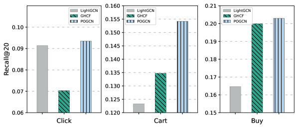
Figure 1. Illustration of the seesaw problems of current multi-behavior collaborative filtering models.

However, encoding the separate multiple behaviors into a joint structure poses the following three challenges:

• Separate Graphs: The current graph concept cannot represent multiple behaviors with one graph. Defining a suitable joint graph to organize arbitrary multiple behaviors is challenging.

• Complicated Behavior Relations: Multiple behaviors can have complex combinations. For instance, users may directly purchase items without favoriting or adding them to the cart. Alternatively, they may add several items to their carts before making a purchase. Therefore, modeling the combination of behaviors is more difficult than modeling individual behaviors.

• Behavior Combination Ordering: Existing models only provide the order of behaviors. It’s challenging to determine the order of behavior combinations such as comparing the order of “buy”, ”click&favor&cart”, and “buy&click”.

In this paper, we tackle the above three challenges by upgrading the infrastructure of multiple behavior graph collaborative filtering and introducing the general Partial Order Graph (POG) to merge separate multi-behavior graphs into a unified one. Specifically, POG utilizes a “graded partial order set” to model all the potential behavior combinations between users and items. Consequently, POG is able to convert any behavior combination into a joint weighted graph. With the help of POG, we propose tailored Partial Order Graph Convolutional Networks (POGCN) to train a single embedding that can benefit multi-behavior recommendation simultaneously. Additionally, we simplify the original multiple-behavior BPR sampling process by developing a tailored partial order BPR sampling strategy. As depicted in Figure.1, POGCN naturally resolves the seesaw problem and improves the recommendation performance on “click”, “cart”, and “buy” simultaneously. Our paper’s primary contributions can be summarized as follows:

• We formally define the partial order graph to describe the complicated behavior combinations to solve the seesaw phenomenon in multi-behavior CF recommendation naturally. Moreover, we prove the completeness of the definition of the partial-order graph that can deal with arbitrary multiple behaviors.

• We propose a novel partial order graph neural network to learn representative single embedding for multi-behavior CF tasks. Besides, we propose a simplified partial order BPR sampling strategy. Detail codes are publicly accessed.

• POGCN has been serving as a core recall model at the homepage of one of the biggest e-commerce platforms—Alibaba, offering accurate and suitable recommendations to over one billion users.

• Extensive experiments on three benchmark datasets present that POGCN outperforms the state-of-the-art multi-behavior methods for above 16.84% Recall, and 19.67% NDCG on average. Online A/B test also demonstrates that POGCN brings 2.02% UCTR and 2.84% GMV improvement in industrial platforms.

2. PRELIMINARY

In this section, we begin by defining the problem of multi-behavior collaborative filtering. We then proceed to introduce the definition of the partial order of behaviors and subsequently define the partial order for combinations of behaviors. Finally, we provide the definition of the graph structure that will be used in subsequent sections, which includes the “separate behavior graph”, the “behavior combination graph”, and our final “partial-order graph (POG)”.

2.1. Notations and Problem Definition

Notations

We use $\mathcal{U}$, $\mathcal{I}$, $\mathcal{B}$, and ${\mathcal{C}}$ to represent the sets of users, items, behaviors, and behavior combination set, respectively. Here, $M$ represents the number of users, $N$ represents the number of items, $K$ represents the number of behavior categories, and $H$ represents the number of behavior combinations. Given ${\mathcal{R}}$ as the set of all interactions of all behaviors, ${\mathcal{R}}_{k}$ denotes the interactions of the $k$-th behavior. Then, describing from the behavior aspect, for each behavior, we have a matrix ${\bm{R}}_{k}$ to describe the interaction of the $k$-th behavior. Specifically, ${\bm{R}}_{k_{ui}}=1$ if user $u$ and item $i$ have the $k$-th behavior, and ${\bm{R}}_{k_{ui}}=0$ if user $u$ and item $i$ do not have the $k$-th behavior. Describing from the users and item interaction aspect, ${\bm{B}}_{ui}=\{b_{ui,1},\dots,b_{ui,K_{ui}}\}$ denotes the set of behaviors between user $u$ and item $i$, and $K_{ui}$ denotes the number of behaviors between user $u$ and item $i$, where $b_{ui,1},\dots,b_{ui,K_{ui}}\in\mathcal{B}$, and ${\bm{B}}_{ui}$ is an element of the behavior combination set ${\mathcal{C}}$.

Multi-behavior Collaborative Filtering (CF)

The ultimate objective of the multi-behavior (embedding-based) collaborative filtering (He et al., 2017; Wang et al., 2019; He et al., 2020) model is to acquire a single representation embedding for each user and item, denoted as ${\bm{E}}_{\mathcal{U}}$ and ${\bm{E}}_{{\mathcal{I}}}$. On a micro level, we utilize ${\bm{e}}_{u}$ and ${\bm{e}}_{i}$ to represent the trained embedding vectors for user $u\in{\mathcal{U}}$ and item $i\in{\mathcal{I}}$.

During the inference step, the relationship between a given user and item pair can be calculated by multiplying their embeddings, $\hat{Y}_{ui}={\bm{e}}_{u}^{\top}\cdot{\bm{e}}_{i}$. Subsequently, for any given user, the online recommender system will rank all the items to filter the most relevant ones. The filtered items for user $u$ can be formally defined as,

(1) $$\hat{{\mathcal{Y}}}_{u}=Filter(\{\hat{Y}_{ui},\ \forall\ i\in{\mathcal{I}},N_{top}\}),$$

where $N_{\text{top}}$ represents the hyperparameter that controls the number of filtered items. During the evaluation process, the recommender system assesses the recommendation performance of all behaviors based on $\hat{{\mathcal{Y}}}_{u}$.

2.2. Definition of Behavior Relations

Partial order of Behaviors

The purpose of proposing a partial order is to address situations where the recommender system cannot determine the order of two or more behaviors. For example, consider the comparison of “favorite”, “share”, and “adding cart”. Previously, the order of behavior definitions would typically treat “favorite”, “share”, and “adding cart” as the same behavior, such as “indirect behavior”, without being able to distinguish between different behaviors. On the other hand, our proposed partial order of behaviors can accommodate ambiguous orders.

Definition 0 (Partial Order of Behaviors).

We define a binary relation $\leq_{b}$ on behavior set ${\mathcal{B}}$, such that for all behaviors $x,y,z\in{\mathcal{B}}$, the following conditions are satisfied:

• Reflexivity: For every $x\in{\mathcal{B}}$, $x\leq_{b}x$.

• Anti-symmetry: For all $x,y\in{\mathcal{B}}$, if $x\leq_{b}y$ and $y\leq_{b}x$, then $x=y$.

• Transitivity: For all $x,y,z\in{\mathcal{B}}$, if $x\leq_{b}y$ and $y\leq_{b}z$, then $x\leq_{b}z$.

After the definition of the partial order of behaviors, the above example can be expressed as the following relation:

$$click\leq_{b}share,favorite,adding\ cart\leq_{b}buy,$$

where “$share,favorite,adding\ cart$” can be called the incomparable relationship in the definition of partial order.

Rank Functions of Behaviors

By defining the partial order of behaviors, we can establish the partial order of behavior combinations based on the nature of the partial order set. To facilitate subsequent numerical computations, we also need to introduce the concept of graded partial order of behaviors.

Definition 0 (Graded Partial Order of Behavior).

The graded partial order of behavior is defined as a partial order set $({\mathcal{B}},\leq_{b})$, augmented with a rank function $\rho_{b}:{\mathcal{B}}\to\mathbb{N}^{+}$, where $\mathbb{N}^{+}$ represents the set of positive natural numbers. The function $\rho_{b}$ satisfies the following conditions:

• Order-Preserving: For all $x,y\in{\mathcal{B}}$, if $x\leq_{b}y$, then $\rho_{b}(x)\leq\rho_{b}(y)$.

• Covering Condition: For all $x,y\in{\mathcal{B}}$, if $y$ covers $x$ (i.e., there is no $z\in{\mathcal{B}}$ such that $x\leq_{b}z\leq_{b}y,$ and $z\neq x,z\neq y$), then $\rho_{b}(y)=\rho_{b}(x)+1$.

With the definition of a graded partial order of behavior, any arbitrary partial order of behaviors can be represented by a corresponding positive integer.

In subsection A.1, we provide the proof of completeness for the grade partial order of behavior combinations to showcase the generality of our definition.

2.3. Definition of Graphs

In this subsection, we formally define the graphs that will be used in the proceeding contents, which are also presented in Figure 2. We begin by discussing the separate behavior graph utilized in related works. Then, we propose the behavior combination graph to depict all combinations of behaviors in a single graph. Finally, we present the partial order graph to assign a rank value to each combination.

Separate Behavior Graphs.

Separate behavior graphs utilize $K$ different graphs to describe each users’ behavior, namely ${\mathcal{G}}_{sep}=\{{\mathcal{G}}_{1},\cdots,{\mathcal{G}}_{K}\}$. For different behaviors $k$, we have corresponding historical interaction information ${\mathcal{R}}_{k}$ between users and items. Therefore, we can represent the corresponding behavior graph of behavior $k$ as ${\mathcal{G}}_{k}=({\mathcal{U}},{\mathcal{I}},{\mathcal{R}}_{k})$. Besides, we utilize ${\bm{R}}_{k}$ to denote the interaction matrix of $k$-th behavior between users and items.

Behavior Combination Graph.

The behavior combination graph’s edges describe the combined behavior situations ${\bm{B}}_{ui}$, representing the set of behaviors occurring between user $u$ and item $i$. For instance, if user $u$ clicks and buys item $i$, then the edge between user $u$ and item $i$ is ${\bm{B}}_{ui}=\{click,buy\}$. In this context, we define the behavior combination graph as ${\mathcal{G}}_{com}=({\mathcal{U}},{\mathcal{I}},{\mathcal{R}})$.

Partial Order Graph.

Since the edges in the behavior combination graph represent discrete set values that cannot be ordered as continuous values, we utilize the rank function in Definition 2 to convert these discrete sets into ordered sets. We refer to this graph as a behavior combination partial order graph or simply a Partial Order Graph (POG). Formally, it is defined as ${\mathcal{G}}_{\text{po}}=({\mathcal{U}},{\mathcal{I}},\rho_{c}({\mathcal{R}}))$, where $\rho_{c}(\cdot)$ denotes the rank function to convert the behavior combinations to integers. ${\bm{R}}$ denotes the interaction matrix of the partial order graph between users and items.

3. METHODOLOGY

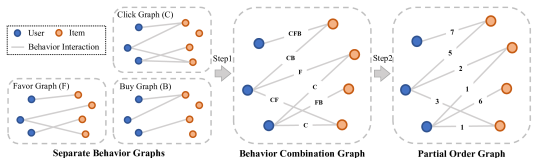
Figure 2. An illustration of the construction of Partial Order Graph (POG). The partial order of behaviors is given as “Click(C) $\leq_{b}$ Favor(F) $\leq_{b}$ Buy(B)”. According to Definition 1, the rank function of the partial order graph can be given as $\rho_{c}(\{\textrm{C, F, B}\})=7$, $\rho_{c}(\{\text{F, B}\})=6$, $\rho_{c}(\{\text{C, B}\})=5$, $\rho_{c}(\{\text{B}\})=4$, $\rho_{c}(\{\text{C, F}\})=3$, $\rho_{c}(\{\text{F}\})=2$, $\rho_{c}(\{\text{C}\})=1$.

In this section, we begin by explaining the process of generating the Partial Order Graph (POG) from the original separate behavior graphs. Subsequently, we delve into the graph convolution on partial order graphs. Lastly, we provide the formula for the partial order BPR loss for multi-behavior CF recommendation.

3.1. Construction of POG

The construction of POG involves one predefinition and one converting step. In the predefinition step, the partial order of behaviors and the partial order of behavior combinations are defined. As depicted in Figure 2, once the orders are defined, separate behavior graphs can be transformed into a behavior combination graph, and subsequently into the partial order graph.

3.1.1. Predefinition

As defined in Definition 1, exports from recommender systems can first define the partial order of behaviors in a customized mode. As shown in Figure 2, considering three behaviors ${\mathcal{B}}=\{click,favor,buy\}$, their partial order $\leq_{b}$ can be defined as “$click\leq_{b}favor\leq_{b}buy$”.

Then, with Definition 2, we can define the rank function $\rho_{c}$ to map any behavior combination ${\mathcal{C}}_{i}$ (subset of the behavior set ${\mathcal{B}}$) to an integer. Specifically, the rank of each set can be defined using the following binary comparison strategy $\leq_{c}$:

Definition 0 (Behavior Combination Binary Relation).

We define a new binary relation $\leq_{c}$ between ${\mathcal{C}}_{i}$ and ${\mathcal{C}}_{j}$. ${\mathcal{C}}_{i}$ and ${\mathcal{C}}_{j}$ represent the behavior combination. For convenience, we define $f(k,\mathcal{C}_{i})$ as the function that returns the number of $k$-ranked behavior ($\rho_{b}(b_{s})=k$) in $\mathcal{C}_{i}$. $f(k,\mathcal{C}_{i})$ can be formally defined as $f(k,\mathcal{C}_{i})=|\{b_{s}\mid\rho_{b}(b_{s})=k,b_{s}\in\mathcal{C}_{i}\}|$, where $||$ denotes the number count function. The relation between behavior combinations can be computed in the following recursion formula:

1. Equality Check: If ${\mathcal{C}}_{i}={\mathcal{C}}_{j}$, then ${\mathcal{C}}_{i}\leq_{c}{\mathcal{C}}_{j}$; otherwise, let $k$ be the max value of $\rho_{b}$, and proceed to the next step.

2. Behavior Intensity Count Comparison: If $f(k,{\mathcal{C}}_{i})<f(k,{\mathcal{C}}_{j})$ (or $f(k,{\mathcal{C}}_{j})<f(k,{\mathcal{C}}_{i})$), then ${\mathcal{C}}_{i}\leq_{c}{\mathcal{C}}_{j}$ (or ${\mathcal{C}}_{j}\leq_{c}{\mathcal{C}}_{i}$ ); otherwise, proceed to the next step.

3. Decrease Intensity: Decrease $k$ by 1 (i.e., $k=k-1$) and repeat from step 2 until $k=1$.

4. Incomparability Determination: If $k=1$ and $f(k,{\mathcal{C}}_{i})=f(k,{\mathcal{C}}_{j})$, then ${\mathcal{C}}_{i}$ and ${\mathcal{C}}_{j}$ are considered incomparable.

With the above definition of “Behavior Combination Binary Relation”, we have the following corollary to demonstrate that the behavior combination set ${\mathcal{C}}$ can also have a rank function to map any given behavior combination to an integer:

Corollary 0.

The set $({\mathcal{C}},\leq_{c})$, when equipped with a rank function $\rho_{c}:{\mathcal{C}}\to\mathbb{N}^{+}$, constitutes a graded partial order set.

A detailed proof of Corollary 2, under complex situations, can be found in Appendix A.1.

Rank function example.

Figure 2 presents a specific example of a rank function. For convenience, we use the abbreviations “B”, “F”, and “C” to represent “buy”, “favor”, and “click” respectively in the presentation of the rank function. Given the partial order set and Definition 1, the rank function of the partial order graph can be defined as follows: $\rho_{c}(\{\text{C, F, B}\})=7$, $\rho_{c}(\{\text{F, B}\})=6$, $\rho_{c}(\{\text{C, B}\})=5$, $\rho_{c}(\{\text{B}\})=4$, $\rho_{c}(\{\text{C, F}\})=3$, $\rho_{c}(\{\text{F}\})=2$, $\rho_{c}(\{\text{C}\})=1$. By examining the rank function, we can observe that “buy” is the most important behavior, and therefore, combinations that include “buy” have a higher rank than those without it. Furthermore, based on the comparison of the most important behavior “buy”, $\{\text{B, F}\}$ has a higher rank than $\{\text{B, C}\}$ because “favor” is considered more important than “click”.

3.1.2. POG Converting

Figure 2 illustrates the entire process of converting the graph from separate behavior graphs to the behavior combination graph and then to the partial order graph. In summary, the behavior combination graph combines all the edges from the separate behavior graphs, where each edge represents a set of behaviors between a specific user and item pair. Afterward, the partial order graph assigns an integer weight to the set of behaviors, resulting in a unified weighted graph.

Specifically, given the definition of the behavior combination between user $u$ and item $i$ as ${\bm{B}}_{ui}$ and the rank function $\rho_{c}(\cdot)$, then the interaction matrix of the partial order graph can be defined as:

(2) $${\bm{R}}_{ui}=\begin{cases}\rho_{c}({\bm{B}}_{ui})^{\tau}&,\text{if }{\bm{B}}_{ui}\neq\phi;\\ 0&,\text{if }{\bm{B}}_{ui}=\phi,\\ \end{cases}$$

where $\tau>0$ represents the temperature coefficient (Van Laarhoven et al., 1987; Bertsimas and Tsitsiklis, 1993) used to adjust the importance weight of various behavior combinations. When $\tau$ is increased, the distance between behavior combinations also increases, while decreasing $\tau$ results in a smaller distance between combinations. If $\tau=0$, the partial order interaction matrix assigns a value of 1 to all interacting user-item pairs, indicating that all behavior combination are considered equally important.

3.2. Partial Order Graph Convolutional Networks

In contrast to GHCF (Chen et al., 2021), MB-CGCN (Cheng et al., 2023), and IMGCF (Zhang et al., 2023), POGCN train a single graph-based CF embedding on the POG. In this section, we first present POGCN in matrix format and then provide the message passing formula to enhance its applicability in industry.

For any given user $u$ and item $i$, we first initialized the original embedding vectors ${\bm{e}}_{u}^{(0)},{\bm{e}}_{i}^{(0)}\in\mathbb{R}^{d}$, where $d$ represents the dimension of the vectors. Then we have an original embedding matrix for all users and items: ${\bm{E}}^{(0)}=[{\bm{e}}^{(0)}_{u_{1}},\dots,{\bm{e}}^{(0)}_{u_{M}},{\bm{e}}^{(0)}_{i_{1}},\dots,{\bm{e}}^{(0)}_{i_{N}}]^{T}$.

Matrix Form

Given the interaction matrix of partial order graph ${\bm{R}}$, we extend the interaction matrix to define the partial order adjacent matrix:

(3) $${\bm{A}}=\begin{bmatrix}0&{\bm{R}}\\ {\bm{R}}^{T}&0\end{bmatrix},$$

then we are able to obtain the partial order graph convolution formula as:

(4) $${\bm{E}}^{(l+1)}=({\bm{D}}^{-\frac{1}{2}}{\bm{A}}{\bm{D}}^{-\frac{1}{2}}){\bm{E}}^{(l)},$$

where ${\bm{D}}\in\mathbb{R}^{(M+N)\times(M+N)}$ is a degree matrix, and ${\bm{D}}_{ii}=\sum_{j}{\bm{A}}_{ij}$, which denotes the sum of $i$-th row value of the partial order adjacent matrix ${\bm{A}}$. With the above definition, the final partial order embedding matrix can be computed as follows:

(5) $${\bm{E}}=\frac{1}{L+1}\sum_{l=0}^{L}{\bm{E}}^{(l)}.$$

After the graph convolution, POGCN will naturally get a single CF embedding to achieve the CF task defined in EQ. (1).

Message Passing Form

The partial order graph can also be done in a neighbor-wise message passing form. Specifically, the $l$-th message passing of user $u$ and item $i$ can be given as:

(6) $${\bm{e}}_{u}^{(l+1)} =\sum_{i\in\mathcal{N}_{u}}\frac{{\bm{R}}_{ui}}{\sqrt{\sum_{t}{\bm{R}}_{ut}}\sqrt{\sum_{t}{\bm{R}}_{ti}}}{\bm{e}}_{i}^{(l)},$$

$${\bm{e}}_{i}^{(l+1)} =\sum_{u\in\mathcal{N}_{i}}\frac{{\bm{R}}_{ui}}{\sqrt{\sum_{t}{\bm{R}}_{ti}}\sqrt{\sum_{t}{\bm{R}}_{ut}}}{\bm{e}}_{u}^{(l)},$$

where $\mathcal{N}_{u}$ and $\mathcal{N}_{i}$ represent the sets of neighboring nodes for user $u$ and item $i$, respectively. $\sum_{t}{\bm{R}}_{ut}$ and $\sum_{t}{\bm{R}}_{ti}$ are the sums of the $u$-th row and the $i$-th column in the partial order interaction matrix ${\bm{R}}$, respectively. $\frac{{\bm{R}}_{ui}}{\sqrt{\sum_{t}{\bm{R}}_{ut}}\sqrt{\sum_{t}{\bm{R}}_{ti}}}$ is the Laplace normalization of message passing in order to avoid numerical instabilities and exploding/vanishing gradients (Kipf and Welling, 2016).

After performing $L$ rounds of propagation, we take the average of the obtained partial order embeddings at each layer to obtain the final representation:

(7) $${\bm{e}}_{u}=\frac{1}{L+1}\sum\limits_{l=0}^{L}{\bm{e}}_{u}^{(l)},{\bm{e}}_{i}=\frac{1}{L+1}\sum\limits_{l=0}^{L}{\bm{e}}_{i}^{(l)},$$

where ${\bm{e}}_{u}$ and ${\bm{e}}_{i}$ represent the final POGCN embedding of user $u$ and item $i$ respectively.

3.3. Partial Order Training Strategy

Bayesian Personalized Ranking (BPR) has been extensively applied in collaborative filtering. Traditional BPR mainly concentrates on training with a single behavior. In this subsection, we introduce an extension called partial order BPR, which aims to achieve efficient and effective multi-behavior collaborative filtering.

Traditional Multi-behavior BPR

Intuitively, one traditional way to combine the BPR loss for multiple behaviors is to apply BPR separately for each behavior and then assign different weights to each behavior. This can be represented as follows:

(8) $${\mathcal{L}}_{ML-BPR}=\sum_{k=1}^{K}\sum_{{\bm{R}}_{k_{ui}}=1}\sum_{{\bm{R}}_{k_{uj}}=0}\alpha_{k}\cdot\ln(\sigma(\hat{Y}_{ui}-\hat{Y}_{uj})),$$

where ${\bm{R}}_{k_{ui}}=1$ indicates that user $u$ and item $i$ have the $k$-th behavior, while ${\bm{R}}_{k_{uj}}=0$ indicates that user $u$ and item $j$ do not have the $k$-th behavior. $\alpha_{k}$ denotes the weight of the $k$-th behavior.

However, the traditional multi-behavior BPR solution has the following limitations: 1. High training cost: Performing BPR training requires computing the embedding for one user and two items, and then performing backpropagation. Therefore, performing traditional multi-behavior BPR will incorporate $K$ times of computational cost of single-behavior BPR, thus increasing the computational complexity. 2. Manual weighting: In traditional solutions, experts have to manually assign the weight, which cannot automatically adapt according to the importance of behavior combinations.

Our POBPR

To overcome these challenges, we propose leveraging a Multinomial Distribution (Murphy, 2012) $P({\mathcal{C}})=P(p_{1},\cdots,p_{H})$ for all $H$ possible behavior combinations, allowing for the sampling of combinations based on their relevance and frequency. Specifically, for any given behavior combination ${\mathcal{C}}_{h}$, the sampling probability is determined as follows:

(9) $$p_{h}=P({\mathcal{C}}_{h})=\frac{\rho_{c}({\mathcal{C}}_{h})^{\gamma}\cdot num({\mathcal{C}}_{h})}{\sum_{j=1}^{H}\rho({\mathcal{C}}_{j})^{\gamma}\cdot num({\mathcal{C}}_{j})},$$

where $num({\mathcal{C}}_{j})$ counts the occurrences of each behavior combination ${\mathcal{C}}_{j}$, and $\gamma$ is a temperature coefficient (Van Laarhoven et al., 1987; Bertsimas and Tsitsiklis, 1993) that moderates the influence of the rank value of each behavior combination.

Table 1. Multi-behavior recommendation performance comparison results. The best and second-best results in each column are highlighted in bold font and underlined, respectively.

Models			MC-BPR	NMTR	GHCF	MB-GMN	MB-CGCN	IMGCF	ESMM	MMoE	PLE	POGCN	Improv. (%)
Beibei	Click	Recall	0.0693	0.0325	0.0703	0.0449	0.0495	0.0688	0.0750	0.0685	0.0614	0.0935	24.68%
		NDCG	0.0560	0.0262	0.0617	0.0360	0.0416	0.0571	0.0652	0.0588	0.0515	0.0841	28.95%
	Cart	Recall	0.1140	0.0702	0.1347	0.0833	0.0945	0.1338	0.1358	0.1240	0.1170	0.1542	13.61%
		NDCG	0.0624	0.0397	0.0812	0.0443	0.0542	0.0758	0.0806	0.0719	0.0672	0.0948	16.78%
	Buy	Recall	0.1428	0.1222	0.1999	0.1220	0.1428	0.1950	0.1680	0.1547	0.1789	0.2029	1.47%
		NDCG	0.0690	0.0619	0.1052	0.0581	0.0724	0.0971	0.0866	0.0777	0.0903	0.1083	3.01%
	Mean	Recall	0.1087	0.0750	0.1350	0.0834	0.0956	0.1326	0.1262	0.1157	0.1191	0.1502	11.28%
		NDCG	0.0624	0.0426	0.0827	0.0461	0.0561	0.0767	0.0775	0.0694	0.0696	0.0957	15.80%
Taobao	Click	Recall	0.0180	0.0016	0.0392	0.0006	0.0018	0.0177	0.0070	0.0014	0.0013	0.0424	8.34%
		NDCG	0.0114	0.0009	0.0274	0.0003	0.0012	0.0113	0.0043	0.0008	0.0008	0.0281	2.46%
	Cart	Recall	0.0276	0.0019	0.0498	0.0012	0.0031	0.0327	0.0141	0.0021	0.0016	0.0555	11.39%
		NDCG	0.0116	0.0006	0.0225	0.0004	0.0016	0.0136	0.0059	0.0007	0.0009	0.0244	8.40%
	Favor	Recall	0.0271	0.0015	0.0595	0.0005	0.0013	0.0277	0.0054	0.0026	0.0011	0.0633	6.52%
		NDCG	0.0116	0.0004	0.0252	0.0003	0.0004	0.0122	0.0021	0.0009	0.0003	0.0261	3.83%
	Buy	Recall	0.0172	0.0027	0.0324	0.0021	0.0008	0.0309	0.0072	0.0005	0.0027	0.0396	22.07%
		NDCG	0.0067	0.0008	0.0155	0.0007	0.0002	0.0128	0.0027	0.0002	0.0015	0.0188	21.04%
	Mean	Recall	0.0225	0.0019	0.0452	0.0011	0.0017	0.0272	0.0084	0.0017	0.0017	0.0502	11.05%
		NDCG	0.0103	0.0007	0.0226	0.0004	0.0009	0.0125	0.0038	0.0006	0.0009	0.0243	7.49%
Tenrec	Click	Recall	0.1284	0.0066	0.1410	0.0102	0.0744	0.0449	0.0108	0.0224	0.0121	0.1627	15.36%
		NDCG	0.0827	0.0038	0.0943	0.0055	0.0511	0.0290	0.0069	0.0137	0.0075	0.1097	16.35%
	Like	Recall	0.1048	0.0105	0.0941	0.0128	0.0756	0.0661	0.0173	0.0222	0.0158	0.1221	16.44%
		NDCG	0.0488	0.0038	0.0393	0.0041	0.0316	0.0325	0.0063	0.0091	0.0076	0.0621	27.33%
	Share	Recall	0.1176	0.0147	0.1029	0.0294	0.0882	0.0772	0.0294	0.0147	0.0404	0.1324	12.50%
		NDCG	0.0399	0.0035	0.0453	0.0091	0.0346	0.0400	0.0095	0.0036	0.0145	0.0636	40.25%
	Follow	Recall	0.0289	0.0051	0.0408	0.0090	0.0405	0.0408	0.0357	0.0204	0.0102	0.0697	70.83%
		NDCG	0.0279	0.0015	0.0225	0.0021	0.0202	0.0162	0.0129	0.0128	0.0034	0.0380	36.25%
	Mean	Recall	0.0949	0.0092	0.0947	0.0154	0.0697	0.0573	0.0233	0.0199	0.0196	0.1217	28.19%
		NDCG	0.0498	0.0031	0.0503	0.0052	0.0344	0.0294	0.0089	0.0098	0.0083	0.0683	35.74%

With the above definition of the categorical distribution, we can provide the complete formula for the POBPR loss as follows:

(10) $$\mathcal{L}_{POBPR}=\mathbb{E}_{{\mathcal{C}}_{h}\sim P({\mathcal{C}})}\left[\sum_{(u,i)\in\mathcal{D}_{h}^{+}}\sum_{j\in\mathcal{D}_{u}^{-}}\ln\sigma(\hat{Y}_{ui}-\hat{Y}_{uj})\right],$$

where $\mathbb{E}_{{\mathcal{C}}_{h}\sim P({\mathcal{C}})}$ represents the expectation over the distribution of behavior combinations, $\mathcal{D}_{h}^{+}$ denotes the sets of positive user-item pairs under the behavior combination ${\mathcal{C}}_{h}$, and $\mathcal{D}_{u}^{-}$ denotes the set of negative items under all interactions of user $u$. We further demonstrate the equivalence between the POBPR and the original separate formula of multi-behavior in terms of the maximum likelihood in Appendix A.2.

4. EXPERIMENTS

In this section, we conduct both offline and online experiments, aiming to answer the following research questions. RQ1: Does POGCN outperform current state-of-the-art models? RQ2: What are the effects of different components in POGCN? RQ3: How does POGCN perform on real-world industrial recommender systems?

4.1. Experimental Setup

4.1.1. Datasets

We conduct comprehensive experiments on three widely used benchmark datasets Beibei (Gao et al., 2019), Taobao (Zhu et al., 2018), and Tenrec (Yuan et al., 2022) including both e-commerce and content recommendation scenarios for offline evaluation to verify the effectiveness and universality of POGCN. The statistics of these datasets are shown in Table 4. In order to avoid the cold start situation of interaction, following previous works (Wang et al., 2019; He et al., 2020), we filter out at least 10 interactive items and users to conduct the experiments. The detailed description of these datasets is illustrated in Appendix B.1.

4.1.2. Compared Baselines

We compare our proposed POGCN with six multi-behavior CF models, three multi-behavior CTR models, and four single-behavior models. (I) Multi-behavior CF models: MC-BPR (Loni et al., 2016), NMTR (Gao et al., 2019), GHCF (Chen et al., 2021), MB-GMN (Xia et al., 2021), MB-CGCN (Cheng et al., 2023), and IMGCF (Zhang et al., 2023). (II) Multi-behavior CTR models: ESMM (Ma et al., 2018a), MMoE (Ma et al., 2018b), and PLE (Tang et al., 2020). (III) Single-behavior CF models: MF-BPR (Rendle et al., 2009), NCF (He et al., 2017), NGCF (Wang et al., 2019), and LightGCN (He et al., 2020). The details of these baseline models are left in Appendix B.2.

4.1.3. Implementation Details

For all models, the embedding size is fixed to 64 and the embedding parameters are initialized with the normal distribution. The learning rate of POGCN is searched from {$1\times 10^{-3},\ 5\times 10^{-4},\ 1\times 10^{-4}$}, the regularization term is searched from {$1\times 10^{-4},\ 5\times 10^{-5},\ 1\times 10^{-5}$}, $\tau$ is searched from [0.2, 1.0] in Taobao and Tenrec with a step of 0.2, and searched from [1.0, 5.0] in Beibei with a step of 1.0, $\gamma$ is searched from [0.2, 2.0] with a step of 0.2. The batch size is set to 1024 for all models and the Adam optimizer (Kingma and Ba, 2014) is used. For multi-behavior CF models, we adopt the partial order relation “click $\leq$ cart $\leq$ buy”, “click $\leq$ cart, favor $\leq$ buy”, and “click $\leq$ like $\leq$ share, follow” for Beibei, Taobao and Tenrec. For multi-behavior CTR models, we replace their backbone with LightGCN to enhance their performance in CF tasks.

4.1.4. Evaluation Metrics

Our evaluation adopts a full-ranking evaluation approach, following the state-of-the-art studies (Wang et al., 2019; He et al., 2020; Krichene and Rendle, 2020). To evaluate the effectiveness of top-ranked articles, we employ Recall@20 and NDCG@20 as our primary metrics for each type of behavior. In order to facilitate the overall comparison across all types of behaviors, we further adopt the mean metric performance of all behaviors for evaluation. Note that we ran all the experiments five times with different random seeds and reported the average results to prevent extreme cases.

4.2. Main Results (RQ1)

In this subsection, we compare our proposed POGCN with state-of-the-art baseline models on the three experimental datasets. The comparison results with multi-behavior CF and CTR models are reported in Table 1, and the comparison results with single-behavior CF models are illustrated in Table 2. From the results, we can have the following observations:

POGCN can achieve significant improvements across all types of behaviors over state-of-the-art methods. From Table 1, we observe that POGCN achieves the highest Recall and NDCG performance across all types of behaviors than both current multi-behavior CF models and multi-behavior recommendation models, with mean NDCG improvements of 15.80%, 7.49%, and 35.74% on Beibei, Taobao, and Tenrec respectively. Furthermore, from Table 2, we can find that POGCN can also generally obtain the best performance through simultaneous multi-behavior learning than single-behavior models with separate training for each behavior. The results verify that POGCN can get better multi-behavior CF recommendation results.

The multi-behavior CF models will negatively affect the performance on click behavior. Comparing the multi-behavior CF models in Table 1 and the traditional single-behavior CF models in Table 2, we can find that the multi-behavior CF models can obtain relatively better results in multiple behaviors recommendation, while they have a performance drop in the click behavior recommendation than the traditional single-behavior CF models. Single-behavior CF models only perform effectively on the click behavior, yielding suboptimal results on other behaviors because they lack training on such data.

The multi-behavior CTR recommendation methods are unsuitable for CF tasks. From the results, we can find that the state-of-the-art multi-behavior recommendation models in CTR scenarios have suboptimal performance in CF scenarios, even if they are equipped with the state-of-the-art LightGCN backbone. Therefore, it is meaningful to design a multi-behavior CF method with our proposed POG and POGCN, which can achieve the best performance for multiple behavior recommendations simultaneously in the collaborative filtering setting. Therefore, it is crucial to propose a multi-behavior model in the CF scenario, which is the motivation of our proposed POGCN.

Table 2. Comparison results with the single behavior recommendation models.

Models			MF-BPR	NCF	NGCF	LightGCN	POGCN
Beibei	Click	Recall	0.0635	0.0837	0.0916	0.0920	0.0935
		NDCG	0.0506	0.0749	0.0819	0.0823	0.0841
	Cart	Recall	0.0808	0.0881	0.1210	0.1233	0.1542
		NDCG	0.0435	0.0475	0.0702	0.0729	0.0948
	Buy	Recall	0.0870	0.1206	0.1534	0.1646	0.2029
		NDCG	0.0415	0.0569	0.0775	0.0841	0.1083
	Mean	Recall	0.0771	0.0975	0.1220	0.1266	0.1502
		NDCG	0.0452	0.0598	0.0766	0.0798	0.0957
Taobao	Click	Recall	0.0191	0.0202	0.0341	0.0421	0.0424
		NDCG	0.0121	0.0120	0.0219	0.0273	0.0281
	Cart	Recall	0.0012	0.0022	0.0062	0.0069	0.0555
		NDCG	0.0004	0.0007	0.0025	0.0033	0.0244
	Favor	Recall	0.0005	0.0032	0.0069	0.0054	0.0633
		NDCG	0.0002	0.0015	0.0028	0.0021	0.0261
	Buy	Recall	0.0013	0.0066	0.0054	0.0059	0.0396
		NDCG	0.0005	0.0030	0.0021	0.0020	0.0188
	Mean	Recall	0.0055	0.0081	0.0132	0.0151	0.0502
		NDCG	0.0033	0.0043	0.0073	0.0087	0.0243
Tenrec	Click	Recall	0.1296	0.1258	0.1537	0.1620	0.1627
		NDCG	0.0834	0.0814	0.1030	0.1097	0.1097
	Like	Recall	0.0032	0.0541	0.0247	0.0277	0.1221
		NDCG	0.0012	0.0289	0.0135	0.0141	0.0621
	Share	Recall	0.0074	0.1103	0.0074	0.0331	0.1324
		NDCG	0.0021	0.0470	0.0018	0.0133	0.0636
	Follow	Recall	0.0153	0.0204	0.0102	0.0204	0.0697
		NDCG	0.0048	0.0058	0.0028	0.0047	0.0380
	Mean	Recall	0.0389	0.0777	0.0490	0.0608	0.1217
		NDCG	0.0229	0.0408	0.0303	0.0355	0.0683

4.3. Ablation Study (RQ2)

In this section, we investigate the effectiveness of the designed components in our method with three model variants: (1) w/o PO-all, which remove all partial order components. We substitute the POG with the interaction graph and treat all interactions with same weight. We also substitute POBPR with traditional BPR sampling. (2) w/o POG, which treats all nodes in the graph with equal weight during graph convolution. (3) w/o POBPR, which utilize traditional BPR sampling instead of POBPR.

We perform ablation studies on Beibei and Taobao datasets, and the outcomes are presented in  Figure 3. Based on the figure, we make the following observations:

• Partial order relation is important for multi-behavior CF recommendation. Substituting the POG and POBPR with the interaction graph and traditional BPR sampling will significantly decrease the CF recommendation performance on all behaviors. This phenomenon verifies that Partial order relation provides a better description of multiple behaviors.

• POG and POBPR are necessary for multi-behavior CF recommendation. From Figure 3, we observe that both POG and POBPR have a positive impact on the performance of multiple behaviors, indicating the importance of constructing customized convolution and training structures.

We also conducted key parameter studies of POGCN, which are placed in Appendix C.1 for reference.

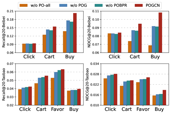
Figure 3. Ablation study results with three POGCN variants.

4.4. Online Evaluation (RQ3)

We conducted an online A/B test on the homepage of Alibaba. In this experiment, our model served as a recall model, replacing the existing online best-performed graph-based recall model—LightGCN. In addition to clicking behavior, POGCN also considers three other valuable behaviors: “adding to cart”, “favoring”, and “buying”. Table 3 presents the average relative performance variation over a successive month for 1.7 billion users and 0.2 billion items.

From the results, we observe that POGCN shows performance improvements of $+1.69\%$ in CVR, $+2.84\%$ in GMV, and $+1.62\%$ in StayTime compared to LightGCN. This indicates that considering deep behaviors such as “adding to cart”, “favor”, and “buy” can enhance the interaction depth and recommendation conversion, thereby increasing the intent of purchasing and viewing more items. Besides, equipped with POGCN, the recommender system is able to provide more accurate recommendations to users, leading to a $+2.83\%$ increase in PCTR and $+2.02\%$ improvement in UCTR. POGCN achieves this through the simultaneous optimization of multiple types of behaviors, thereby enhancing user willingness to click more recommended items.

Therefore, all the A/B testing results validate that $POG$ and the equipped $POGCN$ are more suitable than the state-of-the-art online graph collaborative filtering models.

Table 3. Results of online A/B tests in the industrial platform.

A/B Test	PCTR	UCTR	CVR	GMV	StayTime
v.s. LightGCN	+2.83%	+2.02%	+1.69%	+2.84%	+1.62%

5. RELATED WORKS

5.1. Multi-Behavior Collaborative Filtering

Collaborative filtering recommendation (Su and Khoshgoftaar, 2009; Koren et al., 2021) was originally designed for single-behavior recommendations. Examples of such recommendations include sequence-based (Xue et al., 2017; Huang et al., 2023; Xu et al., 2023) and graph-based (Chen et al., 2020b, 2022; Zhou et al., 2023; Chen et al., 2020a). However, in real-world scenarios, users and items exhibit multiple interaction behaviors (Huang, 2021), such as clicks, purchases, or ratings, instead of focusing solely on a single behavior like clicks (Jin et al., 2020; Cheng et al., 2023; Zhang et al., 2023).

Recent efforts for multi-behavior collaborative filtering mainly focus on utilizing information from multiple types of behaviors for user modeling to enhance recommendation performance for sparse target behaviors, such as using data from clicks, carts, and purchases to model interactions in the purchase behavior domain (Wang et al., 2023; Wei et al., 2022; Xia et al., 2020). Representatively, NMTR (Gao et al., 2019) incorporates a multi-task learning framework that acknowledges the cascading relationship among different user behaviors, allowing for more accurate modeling of user preferences based on a comprehensive set of interactions for target behavior recommendations. Recently, MB-CGCN (Cheng et al., 2023) further employs a sequence of GCN blocks that correspond to different user behaviors to capture the complex dependencies between different user behaviors like views, clicks, and purchases. It enhances recommendation performance by exploiting the cascading nature of these behaviors, where each behavior’s embeddings are transformed and used as input for the next behavior’s embedding learning. Nevertheless, these studies mainly focus on utilizing all types of behaviors to enhance the target behavior performance, while the simultaneous optimization of multiple behaviors has been highly neglected, resulting in poor performance for non-target behaviors.

5.2. Multi-Behavior Click Through Rate Prediction

Multi-behavior CTR prediction models (Zhang and Yang, 2021; Crawshaw, 2020; Bei et al., 2023) aim to effectively model relationships between different recommendation tasks in a multi-task learning framework (Liu et al., 2023; Yan et al., 2023; Wang et al., 2023). These models have achieved state-of-the-art performance in the ranking stage of recommender systems, simultaneously predicting the CTR and CVR.

The most common method of multi-task learning is Shared Bottom (Caruana, 1997), which uses the coupled input to predict each task individually. ESMM (Ma et al., 2018a) utilizes a novel structure that models CVR over the entire space of impressions by employing auxiliary tasks of predicting click-through rate and click-through&conversion rate. MoE (Jacobs et al., 1991), MMoE (Ma et al., 2018b) utilizes a mixture of experts architecture, where each ”expert” is a specialized network in a shared structure, and multiple gating networks then learn to weigh the contribution of each expert for a given task. PLE (Tang et al., 2020) separates shared and task-specific components, employing multi-level experts and gating networks, and introducing a novel progressive separation routing mechanism. This allows PLE to extract deeper, more relevant knowledge for each specific task while mitigating harmful interference between tasks. However, these models are mainly designed for the prediction stage of recommendations. As the previous analyses, they lack the capability to be adopted in the CF stage.

6. CONCLUSION

The introduction of the Partial Order Graphs (POG) and Partial Order Graph Convolutional Networks (POGCN) has significantly advanced the field of multi-behavior collaborative filtering for recommender systems. POGCN offers an update in the infrastructure of multi-behavior CF tasks and presents a groundbreaking solution to the longstanding issue of effectively representing diverse user interactions within a single CF framework. Demonstrating superior performance in both offline experiments and online A/B tests, and practically serving over a billion users in a major shopping platform, POGCN not only elevates the capability of recommendation research but also paves the way for future research and optimizations in the realm of large-scale recommendation systems.

Appendix A Theoretical Details

A.1. Completeness Proof of Partial Order of Behavior Combination

Proof.

We aim to construct a rank function that maps the subsets partitioned from the set ${\mathcal{C}}$ by the binary relation $\leq_{c}$ to a positive integer, thereby establishing $({\mathcal{C}},\leq_{c})$ as a graded partial order set. Define ${\mathcal{C}}_{i}<_{c}{\mathcal{C}}_{j}$ if ${\mathcal{C}}_{i}\leq_{c}{\mathcal{C}}_{j}$ and ${\mathcal{C}}_{i}\neq{\mathcal{C}}_{j}$.

Consider an arbitrary element ${\mathcal{C}}_{i}$ from ${\mathcal{C}}_{j}$. Using the binary relation, we partition ${\mathcal{C}}_{i}$ into three subsets:

• $L_{c}$, containing all ${\mathcal{C}}_{i}$ such that ${\mathcal{C}}_{j}<_{c}{\mathcal{C}}_{i}$,

• $E_{c}$, containing all ${\mathcal{C}}_{j}$ such that ${\mathcal{C}}_{j}={\mathcal{C}}_{i}$ or ${\mathcal{C}}_{i}$ and ${\mathcal{C}}_{j}$ are incomparable,

• $G_{c}$, containing all ${\mathcal{C}}_{j}$ such that ${\mathcal{C}}_{i}<_{c}{\mathcal{C}}_{j}$.

According to Definition 1, for any ${\mathcal{C}}_{j_{1}}\in L_{c}$, ${\mathcal{C}}_{j_{2}}\in E_{c}$, and ${\mathcal{C}}_{j_{3}}\in G_{c}$, it holds that ${\mathcal{C}}_{j_{1}}<_{c}{\mathcal{C}}_{j_{2}}<_{c}{\mathcal{C}}_{j_{3}}$. Elements in $E_{c}$ are considered of equal significance.

This partitioning process is then recursively applied to $L_{c}$ and $G_{c}$ until these sets are empty. Ultimately, we obtain the final partition: $E_{c_{1}},E_{c_{2}},\ldots,E_{c_{n}}$, satisfying ${\mathcal{C}}_{j_{1}}<_{c}{\mathcal{C}}_{j_{2}}<_{c}\cdots<_{c}{\mathcal{C}}_{j_{n}}$ for any ${\mathcal{C}}_{j_{1}}\in E_{c_{1}}$, ${\mathcal{C}}_{j_{2}}\in E_{c_{2}}$, …, ${\mathcal{C}}_{j_{n}}\in E_{c_{n}}$.

Define $\rho_{c}({\mathcal{C}}_{j_{k}})=k$ for all ${\mathcal{C}}_{j_{k}}\in E_{c_{k}}$ and $k=1,2,\ldots,n$. It is evident that $({\mathcal{C}},\leq_{c})$ equipped with $\rho_{c}$ satisfies Definition 2. ∎

A.2. Equivalence Explanation of POBPR

Here, we will explain that such a distribution change is equivalent to transforming the coefficients in the case where behavior combinations are treated as multi-tasks. We have the likelihood function, following BPR (Rendle et al., 2009):

$$L(\theta)=\prod_{{\mathcal{C}}_{h}}\prod_{(u,i,j)\in{\bm{B}}_{{\mathcal{C}}_{h}}\times\mathcal{I}}p(i>_{u}j|\theta),$$

Where ${\bm{B}}_{{\mathcal{C}}_{h}}=\{(u,i)|{\bm{B}}_{ui}={\mathcal{C}}_{h}\}$ represent the interaction set of behavior combination ${\mathcal{C}}_{h}$. For the sake of following discussion, we let $p(i>_{u}j|\theta):=\sigma(\hat{Y}_{ui}(\theta)-\hat{Y}_{uj}(\theta))$, and can get the partial order BPR loss function:

$$\begin{split}\mathcal{L}_{\text{POBPR}}&=\ln p(\Theta|>_{u})\\ &=\ln p(>_{u}|\Theta)p(\Theta)\\ &=\ln\prod_{{\mathcal{C}}_{h}}\prod_{(u,i,j)\in{\bm{B}}_{{\mathcal{C}}_{h}}\times\mathcal{I}}p(i>_{u}j|\theta)+\ln p(\theta)\\ &=\sum_{{\mathcal{C}}_{h}}\sum_{(u,i,j)\in{\bm{B}}_{{\mathcal{C}}_{h}}\times\mathcal{I}}\ln\sigma(\hat{Y}_{ui}(\theta)-\hat{Y}_{uj}(\theta))+\ln p(\theta)\\ &=\sum_{{\mathcal{C}}_{h}}\alpha_{{\mathcal{C}}_{h}}\mathcal{L}_{\text{BPR},{\mathcal{C}}_{h}}+\ln p(\theta),\\ \end{split}$$

where $\alpha_{{\mathcal{C}}_{h}}\propto P({\mathcal{C}}_{h})$ is the coefficient of the behavior combination ${\mathcal{C}}_{h}$ task. So when we change $\gamma$, the coefficients in the multi-task loss function will also change equivalently.

Appendix B Experimental details

B.1. Dataset Details

We adopt three publicly available datasets for offline evaluation. The detailed description of the datasets is as follows:

• Beibei (Gao et al., 2019) is gathered from Beibei platform, one of China’s premier e-commerce platforms specializing in baby products. It encompasses the interactions of 21,716 users and 7,977 items, with three types of user-item behaviors: click, cart, and buy.

• Taobao (Zhu et al., 2018) is a multi-behavior dataset provided by Alibaba, one of the biggest e-commerce platforms in China. It contains the activities (including clicks, carts, favors, and buys) of 26,213 users toward 64,822 items between Nov. 2017 and Dec. 2017.

• Tenrec (Yuan et al., 2022) is a content recommendation dataset collected from two different feeds recommendation apps of Tencent. We utilize the video scenario subset for experiments, with 19,035 users, 15,539 items, and four types of user-item behaviors: click, like, share, and follow.

Details statistics of these datasets are demonstrated in Table 4.

Table 4. Statistics of the experimental datasets.

Datasets	Users	Items	Click	Cart/Like	Favor/Share	Buy/Follow
Beibei	21,716	7,977	2,412,586	642,622	\	304,576
Taobao	26,213	64,822	1,341,843	52,289	23,676	20,880
Tenrec	19,035	15,539	1,367,967	11,295	1,503	1,330

B.2. Baseline Details

We compare our proposed POGCN with thirteen representative state-of-the-art models into three main categories as follows:

(I) Multi-behavior CF models:

• MC-BPR (Loni et al., 2016) utilizes multi-behavior weight to modulate the importance of different behaviors in the BPR loss function.

• NMTR (Gao et al., 2019) is an expansion of NCF (He et al., 2017) in multi-behavior recommendation, adhering to the cascade rule.

• GHCF (Chen et al., 2021) is a graph-based approach for enhancing target behavior recommendation through multi-task learning.

• MB-GMN (Xia et al., 2021) is a graph meta-learning based CF model to improve target behavior recommendations.

• MB-CGCN (Cheng et al., 2023) combines multi-behavior cascade rule to graph convolution networks for target behavior recommendation.

• IMGCF (Zhang et al., 2023) employs a multi-task learning paradigm for CF on multi-behavior graphs, enhancing sparse behavior learning by leveraging information from behaviors with ample data.

(II) Multi-task recommendation models:

• ESMM (Ma et al., 2018a) employs a feature representation transfer learning strategy for multi-task CTR recommendations.

• MMoE (Ma et al., 2018b) adapts the MoE structure to multi-task learning by sharing the expert submodels across all tasks, while also having a gating network trained to optimize each task.

• PLE (Tang et al., 2020) is a progressive layered extraction model with a novel sharing structure design for multi-task CTR recommendations.

(III) Single-behavior CF models:

• MF-BPR (Rendle et al., 2009) is a widely used matrix factorization strategy with the assumption that the positive items should score higher than negative ones.

• NCF (He et al., 2017) is a CF model that leverages a multi-layer perceptron to learn the user–item interaction function.

• NGCF (Wang et al., 2019) explicitly encodes the collaborative signal in the form of high-order connectivities by performing graph embedding propagation.

• LightGCN (He et al., 2020) is a simplified variant of NGCF by including only the most essential components.

Appendix C Additional Experiments

C.1. Parameter Study

C.1.1. Effect of POG Distance Parameter $\tau$

We investigate the effect of the distance parameter $\tau$ of the importance degree between different behaviors with the range of [1.0, 5.0] with a step size of 1.0 for Beibei, and with the range of [0.2, 1.0] with a step size of 0.2 for Taobao. As illustrated in the upper side of Figure 4, the best value of $\tau$ for Beibei is 3.0, while the best $\tau$ value for Taobao is 0.2. Therefore, the selection of parameter $\tau$ should be considered carefully for better POGCN performance.

C.1.2. Effect of Sampling Distance Parameter $\gamma$

We also evaluate the impact of different partial order sampling distance values of $\gamma$, with the range of [0.2, 2.0] with a step size of 0.2. From the second row of Figure 4, we can find that the too-small $\gamma$ value will lead to too similar between different behaviors and lead to suboptimal performance. The selection of the $\gamma$ value is contingent upon the specific characteristics of each dataset, necessitating a careful choice to optimize performance. For instance, an $\gamma$ value of 1.4 is well-suited for the Beibei dataset, whereas a lower value of 0.6 is preferable for the Taobao dataset.

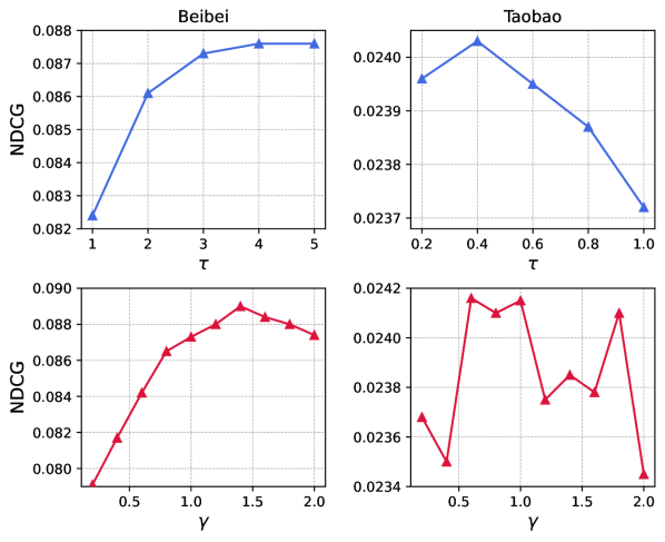
Figure 4. Parameter study of $\tau$ and $\gamma$ on Beibei and Taobao over the Mean NDCG metric.

References

- (1)
- Bei et al. (2023) Yuanchen Bei, Hao Chen, Shengyuan Chen, Xiao Huang, Sheng Zhou, and Feiran Huang. 2023. Non-Recursive Cluster-Scale Graph Interacted Model for Click-Through Rate Prediction. In Proceedings of the 32nd ACM International Conference on Information and Knowledge Management. 3748–3752.
- Bertsimas and Tsitsiklis (1993) Dimitris Bertsimas and John Tsitsiklis. 1993. Simulated annealing. Statistical science 8, 1 (1993), 10–15.
- Caruana (1997) Rich Caruana. 1997. Multitask learning. Machine learning 28 (1997), 41–75.
- Chen et al. (2021) Chong Chen, Weizhi Ma, Min Zhang, Zhaowei Wang, Xiuqiang He, Chenyang Wang, Yiqun Liu, and Shaoping Ma. 2021. Graph heterogeneous multi-relational recommendation. In Proceedings of the AAAI Conference on Artificial Intelligence, Vol. 35. 3958–3966.
- Chen et al. (2024) Hao Chen, Yuanchen Bei, Qijie Shen, Yue Xu, Sheng Zhou, Wenbing Huang, Feiran Huang, Senzhang Wang, and Xiao Huang. 2024. Macro Graph Neural Networks for Online Billion-Scale Recommender Systems. arXiv preprint arXiv:2401.14939 (2024).
- Chen et al. (2022) Hao Chen, Zhong Huang, Yue Xu, Zengde Deng, Feiran Huang, Peng He, and Zhoujun Li. 2022. Neighbor enhanced graph convolutional networks for node classification and recommendation. Knowledge-Based Systems 246 (2022), 108594.
- Chen et al. (2020b) Hao Chen, Yue Xu, Feiran Huang, Zengde Deng, Wenbing Huang, Senzhang Wang, Peng He, and Zhoujun Li. 2020b. Label-Aware Graph Convolutional Networks. In Proceedings of the 29th ACM International Conference on Information & Knowledge Management. 1977–1980.
- Chen et al. (2020a) Lei Chen, Le Wu, Richang Hong, Kun Zhang, and Meng Wang. 2020a. Revisiting graph based collaborative filtering: A linear residual graph convolutional network approach. In Proceedings of the AAAI conference on artificial intelligence, Vol. 34. 27–34.
- Cheng et al. (2023) Zhiyong Cheng, Sai Han, Fan Liu, Lei Zhu, Zan Gao, and Yuxin Peng. 2023. Multi-Behavior Recommendation with Cascading Graph Convolution Networks. In Proceedings of the ACM Web Conference 2023. 1181–1189.
- Crawshaw (2020) Michael Crawshaw. 2020. Multi-task learning with deep neural networks: A survey. arXiv preprint arXiv:2009.09796 (2020).
- Gao et al. (2019) Chen Gao, Xiangnan He, Dahua Gan, Xiangning Chen, Fuli Feng, Yong Li, Tat-Seng Chua, and Depeng Jin. 2019. Neural multi-task recommendation from multi-behavior data. In 2019 IEEE 35th international conference on data engineering (ICDE). IEEE, 1554–1557.
- Guo et al. (2020) Qingyu Guo, Fuzhen Zhuang, Chuan Qin, Hengshu Zhu, Xing Xie, Hui Xiong, and Qing He. 2020. A survey on knowledge graph-based recommender systems. IEEE Transactions on Knowledge and Data Engineering 34, 8 (2020), 3549–3568.
- He et al. (2020) Xiangnan He, Kuan Deng, Xiang Wang, Yan Li, Yongdong Zhang, and Meng Wang. 2020. Lightgcn: Simplifying and powering graph convolution network for recommendation. In Proceedings of the 43rd International ACM SIGIR conference on research and development in Information Retrieval. 639–648.
- He et al. (2017) Xiangnan He, Lizi Liao, Hanwang Zhang, Liqiang Nie, Xia Hu, and Tat-Seng Chua. 2017. Neural collaborative filtering. In Proceedings of the 26th international conference on world wide web. 173–182.
- Huang (2021) Chao Huang. 2021. Recent advances in heterogeneous relation learning for recommendation. arXiv preprint arXiv:2110.03455 (2021).
- Huang et al. (2023) Feiran Huang, Zefan Wang, Xiao Huang, Yufeng Qian, Zhetao Li, and Hao Chen. 2023. Aligning Distillation For Cold-Start Item Recommendation. In Proceedings of the 46th International ACM SIGIR Conference on Research and Development in Information Retrieval. 1147–1157.
- Jacobs et al. (1991) Robert A Jacobs, Michael I Jordan, Steven J Nowlan, and Geoffrey E Hinton. 1991. Adaptive mixtures of local experts. Neural computation 3, 1 (1991), 79–87.
- Jin et al. (2020) Bowen Jin, Chen Gao, Xiangnan He, Depeng Jin, and Yong Li. 2020. Multi-behavior recommendation with graph convolutional networks. In Proceedings of the 43rd International ACM SIGIR Conference on Research and Development in Information Retrieval. 659–668.
- Kingma and Ba (2014) Diederik P Kingma and Jimmy Ba. 2014. Adam: A method for stochastic optimization. arXiv preprint arXiv:1412.6980 (2014).
- Kipf and Welling (2016) Thomas N Kipf and Max Welling. 2016. Semi-supervised classification with graph convolutional networks. arXiv preprint arXiv:1609.02907 (2016).
- Koren et al. (2021) Yehuda Koren, Steffen Rendle, and Robert Bell. 2021. Advances in collaborative filtering. Recommender systems handbook (2021), 91–142.
- Krichene and Rendle (2020) Walid Krichene and Steffen Rendle. 2020. On sampled metrics for item recommendation. In Proceedings of the 26th ACM SIGKDD international conference on knowledge discovery & data mining. 1748–1757.
- Liu et al. (2023) Qi Liu, Zhilong Zhou, Gangwei Jiang, Tiezheng Ge, and Defu Lian. 2023. Deep Task-specific Bottom Representation Network for Multi-Task Recommendation. In Proceedings of the 32nd ACM International Conference on Information and Knowledge Management. 1637–1646.
- Loni et al. (2016) Babak Loni, Roberto Pagano, Martha Larson, and Alan Hanjalic. 2016. Bayesian personalized ranking with multi-channel user feedback. In Proceedings of the 10th ACM conference on recommender systems. 361–364.
- Ma et al. (2018b) Jiaqi Ma, Zhe Zhao, Xinyang Yi, Jilin Chen, Lichan Hong, and Ed H Chi. 2018b. Modeling task relationships in multi-task learning with multi-gate mixture-of-experts. In Proceedings of the 24th ACM SIGKDD international conference on knowledge discovery & data mining. 1930–1939.
- Ma et al. (2018a) Xiao Ma, Liqin Zhao, Guan Huang, Zhi Wang, Zelin Hu, Xiaoqiang Zhu, and Kun Gai. 2018a. Entire space multi-task model: An effective approach for estimating post-click conversion rate. In The 41st International ACM SIGIR Conference on Research & Development in Information Retrieval. 1137–1140.
- Murphy (2012) Kevin P Murphy. 2012. Machine learning: a probabilistic perspective. MIT press.
- Rendle et al. (2009) Steffen Rendle, Christoph Freudenthaler, Zeno Gantner, and Lars Schmidt-Thieme. 2009. BPR: Bayesian personalized ranking from implicit feedback. In Proceedings of the Twenty-Fifth Conference on Uncertainty in Artificial Intelligence. 452–461.
- Su and Khoshgoftaar (2009) Xiaoyuan Su and Taghi M Khoshgoftaar. 2009. A survey of collaborative filtering techniques. Advances in artificial intelligence 2009 (2009).
- Tang et al. (2020) Hongyan Tang, Junning Liu, Ming Zhao, and Xudong Gong. 2020. Progressive layered extraction (ple): A novel multi-task learning (mtl) model for personalized recommendations. In Proceedings of the 14th ACM Conference on Recommender Systems. 269–278.
- Van Laarhoven et al. (1987) Peter JM Van Laarhoven, Emile HL Aarts, Peter JM van Laarhoven, and Emile HL Aarts. 1987. Simulated annealing. Springer.
- Wang et al. (2021) Shoujin Wang, Liang Hu, Yan Wang, Xiangnan He, Quan Z Sheng, Mehmet A Orgun, Longbing Cao, Francesco Ricci, and Philip S Yu. 2021. Graph learning based recommender systems: A review. arXiv preprint arXiv:2105.06339 (2021).
- Wang et al. (2019) Xiang Wang, Xiangnan He, Meng Wang, Fuli Feng, and Tat-Seng Chua. 2019. Neural graph collaborative filtering. In Proceedings of the 42nd international ACM SIGIR conference on Research and development in Information Retrieval. 165–174.
- Wang et al. (2023) Yuhao Wang, Ha Tsz Lam, Yi Wong, Ziru Liu, Xiangyu Zhao, Yichao Wang, Bo Chen, Huifeng Guo, and Ruiming Tang. 2023. Multi-Task Deep Recommender Systems: A Survey. arXiv preprint arXiv:2302.03525 (2023).
- Wei et al. (2022) Wei Wei, Chao Huang, Lianghao Xia, Yong Xu, Jiashu Zhao, and Dawei Yin. 2022. Contrastive meta learning with behavior multiplicity for recommendation. In Proceedings of the fifteenth ACM international conference on web search and data mining. 1120–1128.
- Wu et al. (2021) Jiancan Wu, Xiang Wang, Fuli Feng, Xiangnan He, Liang Chen, Jianxun Lian, and Xing Xie. 2021. Self-supervised graph learning for recommendation. In Proceedings of the 44th international ACM SIGIR conference on research and development in information retrieval. 726–735.
- Wu et al. (2022) Shiwen Wu, Fei Sun, Wentao Zhang, Xu Xie, and Bin Cui. 2022. Graph neural networks in recommender systems: a survey. Comput. Surveys 55, 5 (2022), 1–37.
- Xia et al. (2020) Lianghao Xia, Chao Huang, Yong Xu, Peng Dai, Bo Zhang, and Liefeng Bo. 2020. Multiplex behavioral relation learning for recommendation via memory augmented transformer network. In Proceedings of the 43rd international ACM SIGIR conference on research and development in information retrieval. 2397–2406.
- Xia et al. (2021) Lianghao Xia, Yong Xu, Chao Huang, Peng Dai, and Liefeng Bo. 2021. Graph meta network for multi-behavior recommendation. In Proceedings of the 44th international ACM SIGIR conference on research and development in information retrieval. 757–766.
- Xu et al. (2023) Yue Xu, Hao Chen, Zefan Wang, Jianwen Yin, Qijie Shen, Dimin Wang, Feiran Huang, Lixiang Lai, Tao Zhuang, Junfeng Ge, and Xia Hu. 2023. Multi-Factor Sequential Re-Ranking with Perception-Aware Diversification. In Proceedings of the 29th ACM SIGKDD Conference on Knowledge Discovery and Data Mining. 5327–5337.
- Xue et al. (2017) Hong-Jian Xue, Xinyu Dai, Jianbing Zhang, Shujian Huang, and Jiajun Chen. 2017. Deep matrix factorization models for recommender systems.. In IJCAI, Vol. 17. Melbourne, Australia, 3203–3209.
- Yan et al. (2023) Mingshi Yan, Zhiyong Cheng, Chen Gao, Jing Sun, Fan Liu, Fuming Sun, and Haojie Li. 2023. Cascading residual graph convolutional network for multi-behavior recommendation. ACM Transactions on Information Systems (2023).
- Yu et al. (2022) Junliang Yu, Hongzhi Yin, Xin Xia, Tong Chen, Lizhen Cui, and Quoc Viet Hung Nguyen. 2022. Are graph augmentations necessary? simple graph contrastive learning for recommendation. In Proceedings of the 45th international ACM SIGIR conference on research and development in information retrieval. 1294–1303.
- Yuan et al. (2022) Guanghu Yuan, Fajie Yuan, Yudong Li, Beibei Kong, Shujie Li, Lei Chen, Min Yang, Chenyun Yu, Bo Hu, Zang Li, et al. 2022. Tenrec: A Large-scale Multipurpose Benchmark Dataset for Recommender Systems. Advances in Neural Information Processing Systems 35 (2022), 11480–11493.
- Zhang et al. (2023) Yijie Zhang, Yuanchen Bei, Shiqi Yang, Hao Chen, Zhiqing Li, Lijia Chen, and Feiran Huang. 2023. Alleviating Behavior Data Imbalance for Multi-Behavior Graph Collaborative Filtering. In 2023 IEEE International Conference on Data Mining Workshops (ICDMW).
- Zhang and Yang (2021) Yu Zhang and Qiang Yang. 2021. A survey on multi-task learning. IEEE Transactions on Knowledge and Data Engineering 34, 12 (2021), 5586–5609.
- Zhou et al. (2023) Huachi Zhou, Hao Chen, Junnan Dong, Daochen Zha, Chuang Zhou, and Xiao Huang. 2023. Adaptive Popularity Debiasing Aggregator for Graph Collaborative Filtering. In Proceedings of the 46th International ACM SIGIR Conference on Research and Development in Information Retrieval. 7–17.
- Zhu et al. (2018) Han Zhu, Xiang Li, Pengye Zhang, Guozheng Li, Jie He, Han Li, and Kun Gai. 2018. Learning tree-based deep model for recommender systems. In Proceedings of the 24th ACM SIGKDD International Conference on Knowledge Discovery & Data Mining. 1079–1088.