Evaluation of plasma on deflection angle and shadow by a black hole solution immersed in perfect fluid in Rastall theory

Abstract

The present study examines the gravitational deflection of particles in curved space-times immersed in perfect fluid in the context of Rastall theory, applying the Gibbons-Werner useful technique. In its application to integral areas inside a four-dimensional space-time, the Gauss-Bonnet theorem studies the computation expression of the deflection angle. The Gibbons-Werner technique has two limitations in Rastall theory for space-times immersed in perfect fluid: the integral region is generally infinite and the integral complicates calculation, particularly for complex space-times and extremely accurate solutions. An infinite region approach to Gibbons-Werner is proposed to avoid singularity. For demonstrating the Gibbons-Werner method, we use a complete Rastall theory framework. It studies black hole solutions like the dust field, radiation field, quintessence field, cosmological constant field and phantom field using the Gibbons-Werner approach. Additionally, we check the deflection angle from these space-times under the influence of plasma. Furthermore, we compute analytically the influence of a plasma on a black hole shadow by using a ray-tracing approach. In the Hamiltonian equation, our model describes the plasma, so the light ray motion equations are independent of the plasma’s velocity. It is assumed that plasma is a dispersive medium, pressure-less and non-magnetized. We investigate the perfect fluid in Rastall theory in further depth, where the plasma particle density corresponds to particle accumulation. The supermassive black hole shadows are explored in the case when plasma falls radially from infinity onto a black hole.

I Introduction

In general relativity (GR), one of the most significant fields of study is the movement of objects in intense gravitational fields. An object’s path can be examined using the geodesic expression of the intense gravitational field. By considering it as a test particle, its gravitational field is ignorable. An important consideration in observing the test particle’s velocity is the trajectory’s deflection. In general, there are two types of particles: massive particles and massless particles, especially photons. Gravitational theories R1 such as GR are verified in significant part for massless particles through gravitational deflection. Many techniques have been suggested R2 -R22 to study the deflection angle (DA) of photons. For massive particles, they may function as representatives of all that exists. Later on, Eddington’s detection justified R23 the deflection of light moving by the sun. Gravitational lensing has been extensively studied as a powerful tool in various fields of cosmology and astronomy. For neutrinos, gravitons, neutrons and celestial events of high energy ($\pi$-mesons, K-mesons, $\mu$ons, etc.) are examples. There are also theoretically weakly associating massive particles and their axions R24 . Important details as to the source, lens, trajectory context, and particles can actually be obtained from the gravitational deflection of these significant particles R25 ; R26 ; R27 ; R28 ; R29 ; R30 ; R31 ; R32 ; R33 ; R34 ; R35 ; R36 . The Gibbons-Werner (GW) approach, originally proposed by Gibbons-Werner in 2008 R36 and then modified by scientists in more recent times R37 ; R38 ; R39 ; R40 ; R41 ; R43 ; R44 , helps in the geometric explanation and determination of the DA for both massless and massive particles. The development of a four-dimensional spacetime that can be utilised to explain the motion and integral region of the particle on a two-dimensional Riemann manifold, the trajectory of the particle, an auxiliary circular curve, a radial upward curve that passes through the source, and a radial outward curve that passes through the observer are all part of the fundamental technique of the GW approach. The Gauss-Bonnet theorem (GBT) can be applied to the integral region for the DA in the form of geometric parameters.

Consider a black hole (BH), which has a consistent spacetime structure but can be lighted by external electromagnetic radiation with varying shapes, colours, and behaviours throughout time. The BH can be detected by many mathematical approaches, but its impact on light distribution can be observed. The Event Horizon Telescope Collaboration R45 appears as the first image of a BH. The image shows a continuous spacetime structure illuminated by a time-varying emission zone, encouraging more investigation and explanation. Several of the concepts employed by the Event Horizon Telescope (EHT), such as BH shadows, have been given multiple explanations in the literature. In R46 , Synge calculated the angular radius of the Schwarzschild BH’s shadow using a static observer model. The investigation has been done on the various geometries of BH shadows in Refs R47 -R76 . As the magnetic field parameter grows, the shadows of the Schwarzschild and Kerr BHs immersed in the Melvin magnetic field grow and elongate in a horizontal direction. Black hole shadows can only be predicted by employing a ray-tracing approach R57 ; R58 ; R62 for light motion systems with non-integrability.

However,the work has focused on the direct local effects of cosmic models on the known BH solutions. Babichev et al. R77 demonstrate that in a scenario with a phantom field, the accreting particles of the phantom scalar field into the central BH cause the BH mass to decrease. But this does have a broad influence. A modified metric that includes the BHs surrounding spacetime can be used to determine the local changes in the spacetime geometry surrounding the fundamental BH. In this context, Kiselev R78 has achieved an analytically static, spherically symmetric solution to Einstein’s equations. The basis of the Rastall theory is related to high-curvature situations; hence, the physics of BHs may provide a suitable framework for further exploration of this theory. Thus, as a novel class of non-vacuum BH solutions to this theory, our goal in this study is to find the surrounding Kiselev-like BH solutions. The properties of the BHs surrounding fields, which are typically such as radiation, dust, or a dark energy component, define this solution R78 ; R79 . The Kiselev every field solution’s special cases (a) Schwarzschild BH encompassed by quintessence, BH encompassed by magnetised Ernst field and a Reissner-Nordstrom BH encircled by radiation and dust (b), as well as its phase changes and thermodynamical quantities are examined in R79 ; R80 and R81 describes the dynamics of a neutral and a charged particle surrounding the Schwarzschild black encircled by quintessence matter.

In order to avoid spacetime singularity, one of the main reasons to research the BH surrounding field in Rastall theory. Although there is a well-developed Rastall theory at this point, there are numerous attempts, such as black rings field theory and BH geometry. The expectation that there should be an intrinsic extended structure in spacetime is acknowledged by almost all of this approach (Gibbons-Werner approach). Stable-orbit photons are in constant motion around a BH; they are unable to leave the BH or travel to infinity. In this instance, the prograde stable photon orbits correspond to the dark region that only partially emerges from the main shadow. The BH shadow is half-panoramic (equatorial), due to the lack of backward unstable (stable) light rings. In this instance, the BH shadow turns into an equatorial, panoramic shadow without a grey area for stable photon orbits. The expectation that there should be an intrinsic extended structure in spacetime is acknowledged by almost all of this approach (ray-tracing approach). It is studied that the BH shadows are immersed in charge fields and that the BH shadow is affected by the perfect fluid in the context of Rastall theory.

This is way the paper is formatted. Section $2$ discusses an overview of the analytical technique for spherically symmetric BHs in Rastall theory. Section $3$ study the DA for BHs occupied by dust, quintessence, radiation, phantom fields and cosmological constant and also their graphical analysis. In section $4$, we investigate the results of DA and graphical behavior in the background of plasma frame for associated BHs. Section $5$ comprises the shadow cast and contour plots for BHs surrounded by dust, quintessence, radiation, phantom fields and cosmological constant. In section $6$, we summarize the results of our work.

II Introductory Review of black hole in the background of Rastall Theory

Within the framework of the Rastall theory of gravity, we seek the general non-vacuum spherically symmetric static uncharged BH solutions in this section. Utilizing Rastall’s idea R82 ; R83 ; A1 , we obtain the following for a spacetime where an energy-momentum source of $T_{ab}$ occupies the Ricci scalar $R$ as

$$\lambda R^{,b}=T^{ab};a,$$ (1)

with $\lambda$ represents the Rastall parameter, which is the conventional GR conservation law that has deviated. The Rastall field equations can be expressed as

$$kT_{ab}=G_{ab}+k\lambda g_{ab}R,$$ (2)

where the gravitational constant of Rastall coupling is denoted by $k$. In the limit of $\lambda\rightarrow 0$ and $k=8\pi G$, these field equations reduce to GR field equations, with $G$ is the gravitational constant of Newton coupling. To derive BH solutions, we take the usual Schwarzschild coordinates general spherical symmetric metric as A1

$$ds^{2}=-A(r)dt^{2}+\frac{dr^{2}}{A(r)}+r^{2}d\Omega^{2},$$ (3)

with the two-dimensional unit sphere is represented by the equation $d\Omega^{2}=d\theta^{2}+\sin^{2}\theta d\phi^{2}$, and $f(r)$ is a fundamental metric function that depends on the radial coordinate. We can derive non-vanishing components of the Rastall tensor, defined as $H_{ab}=G_{ab}+k\lambda g_{ab}R$, can be followed by applying this metric, we get A1

$$H^{0}_{0} = G^{0}_{0}+k\lambda R=-\frac{1}{A}G_{00}+k\lambda R=\frac{1}{r^{2}}(\acute{A}r-1+A)+k\lambda R,$$

$$H^{1}_{1} = G^{1}_{1}+k\lambda R=AG_{11}+k\lambda R=\frac{1}{r^{2}}(\acute{A}r-1+A)+k\lambda R,$$

$$H^{2}_{2} = G^{2}_{2}+k\lambda R=-\frac{1}{r^{2}}G_{22}+k\lambda R=\frac{1}{r^{2}}(\acute{A}r+\frac{1}{2}r^{2}\acute{\acute{A}})+k\lambda R,$$

$$H^{3}_{3} = G^{3}_{3}+k\lambda R=-\frac{1}{r^{2}\sin^{2}\theta}G_{33}+k\lambda R=\frac{1}{r^{2}}(\acute{A}r+\frac{1}{2}r^{2}\acute{\acute{A}})+k\lambda R.$$ (4)

In this case, the Ricci scalar is defined as

$$R=-\frac{1}{r^{2}}(r^{2}\acute{\acute{A}}+4r\acute{A}+2+2A),$$ (5)

with the derivative with regard to the radial coordinate r is represented by the prime sign. In relation to the Rastall tensor ($H^{a}_{b}$) non-vanishing components, then the following diagonal form should be present in the entire energy-momentum tensor that governs this spacetime.

$$T^{a}_{b}=\begin{pmatrix}T^{0}_{0}&0&0&0\\ 0&T^{1}_{1}&0&0\\ 0&0&T^{2}_{2}&0\\ 0&0&0&T^{3}_{3}\end{pmatrix},$$ (6)

with it is satisfied with the Rastall tensor $H^{a}_{b}$ symmetry features. With respect to solutions of Rastall tensor, the equality conditions $H^{0}_{0}=H^{1}_{1}$ and $H^{2}_{2}=H^{3}_{3}$ must also have $T^{0}_{0}=T^{1}_{1}$ and $T^{2}_{2}=T^{3}_{3}$, respectively. After that, a general energy and momentum tensor T with these symmetry features can be generated in the manner shown as

$$T^{a}_{b}=\tau^{a}_{b}+E^{a}_{b},$$ (7)

with $E^{a}_{b}$ is the trace free of Maxwell tensor defined by

$$E^{a}_{b}=\frac{2}{k}(F_{a\mu}F^{\mu}_{b}-\frac{1}{4}g_{ab}F^{\mu\nu}F_{{\mu\nu}}).$$ (8)

So that $F_{ab}$ represents the anti-symmetric Faraday tensor obeying the corresponding vacuum Maxwell expression as

$$F^{ab}_{;a} = 0,$$

$$\partial[\alpha F_{ab}] = 0.$$ (9)

Given that the spacetime metric (3) has spherical symmetry, the only non-vanishing Faraday tensor $F^{ab}$ of components is imposed to be $F^{01}=-F^{10}$. Next, using the equations in (9), one can get

$$F^{01}=\frac{Q}{r^{2}},$$ (10)

where $Q$ represents an integration constant behaving as an electrostatic charge, the only Maxwell tensor $E^{a}_{b}$ non-vanishing components are given by equations (3), (8), and (10) as

$$E^{a}_{b}=\frac{Q^{2}}{kr^{4}}\textit{diagonal}(-1,-1,1,1),$$ (11)

possessing the symmetries in the $H^{a}_{b}$ tensor and evidently expressing an electrostatic field. Conversely, $\tau^{a}_{b}$ denotes the surrounding field’s energy–momentum tensor, which is defined R84 as

$$\tau^{0}_{0} = -\rho_{s}(r)$$

$$\tau^{j}_{i} = -\rho_{s}(r)\mu\big{(}-\frac{r_{j}r^{i}}{r_{n}r^{n}}-3\nu\frac{r_{j}r^{i}}{r_{n}r^{n}}+\nu\delta^{j}_{i}\big{)}.$$ (12)

With respect to the arbitrary parameters $\mu$ and $\nu$, which correspond to the internal structure of the BH surrounding the field, this model of $\tau^{a}_{b}$ implies that the space component is proportionate to the time category, which represents the energy density. The surrounding field in this case is indicated by the subscript (s), which is usually any combination of dust, radiation, quintessence, cosmological constant, and phantom field. We can determine the isotropic average over the angles by using R84 the

$$<\tau^{j}_{i}>=\frac{1}{3}\rho_{s}\delta^{j}_{i}=\rho_{s}\delta^{j}_{i},$$ (13)

as it is assumed that $<r^{j}r_{i}>=\frac{\mu}{3}\rho_{s}\delta^{j}_{i}r_{n}r^{n}.$ The barotropic expression of equilibrium for the surrounding field thus becomes

$$p_{s}=\rho_{s}\omega_{s},~{}~{}~{}~{}\omega_{s}=\frac{\mu}{3},$$ (14)

with $\omega_{s}$ and $\rho_{s}$ indicate the equation of the state parameter and the pressure, respectively. The principle of the addition and linearity scenario assumed in reference R84 to find the free parameter $\nu$ of the energy momentum tensor of the surrounding field as suggested is thus precisely provided by the field expressions (4) with respect to the entire energy-momentum tensor in (7), (11) and (12) as

$$\nu=-\frac{3\omega_{s}+1}{6\omega_{s}}.$$ (15)

Then, the following form can be used to derive the non-vanishing components of the $\tau_{ab}$ tensor

$$\tau^{0}_{0} = \tau^{1}_{1}=-\rho_{s}$$

$$\tau^{2}_{2} = \tau^{3}_{3}=\frac{1}{2}(3\omega_{s}+1)\rho_{s},$$ (16)

which in the Rastall tensor $H^{a}_{b}$ also have identical symmetries. Consequently, all of $H^{a}_{b}$ symmetry is admitted by our whole constructed energy-momentum tensor in (7). The Rastall field equations $\tau^{a}_{b}$ can be regarded as the only energy-momentum tensor of assistance. The solutions produced will thus explain the encircled uncharged BH solutions in the Rastall theory context, which are not the same as the ones in GR. Within the context of this theory, the most generic class of static surrounding charged BH solutions can be obtained by including the Maxwell tensor $E^{a}_{b}$ in $T^{a}_{b}$. The field equations are solved and their general solution is obtained in the following. Next, we tackle the two uncharged/charged solutions. From the $H^{0}_{0}=T^{0}_{0}$ and $H^{1}_{1}=T^{1}_{1}$ components of the Rastall field expression, the differential equation that follows is obtained as

$$\frac{1}{r^{2}}(r\acute{A}+A-1)-\frac{k\lambda}{r^{2}}(r^{2}\acute{\acute{A}}+4r\acute{A}+2\acute{A}-2)=-\frac{Q^{2}}{r^{4}}-k\rho_{s},$$ (17)

and $H^{2}_{2}=T^{2}_{2}$ and $H^{3}_{3}=T^{3}_{3}$ components are interpreted as

$$\frac{1}{r^{2}}(r\acute{A}+\frac{1}{2}r^{2}\acute{\acute{A}})-\frac{k\lambda}{r^{2}}(r^{2}\acute{\acute{A}}+4r\acute{A}+2A-2)=-\frac{Q^{2}}{r^{4}}+\frac{k\rho_{s}}{2}(1+3\omega_{s}),$$ (18)

As a result A1 , the two differential equations (17) and (18) allow us to analytically compute the one unknown functions $A(r)$ as

$$A(r)=1-\frac{2M}{r}+\frac{Q^{2}}{r^{2}}-\frac{N_{s}}{r^{\frac{1-3\omega_{s}-6k\lambda(1+\omega_{s})}{1-3k\lambda(1+\omega_{s})}}},$$ (19)

where the BH mass and the surrounding field structure parameter are represented by two integration constants, $M$ and $N_{s}$, respectively. The parameters $k$ and $\lambda$ represents the Rastall geometric parameters and $\omega_{s}$ denotes the equation of state parameter of BH surrounding field. Keep in mind that the characteristics of the surrounding field are represented by the integration constant $N_{s}$. Any combination of $k$, $\lambda$ and $\omega_{s}$ parameters can accept various positive or negative $N_{s}$ values. We recover the Reissner-Nordström BH occupied by a surrounding field in GR, which was initially discovered by Kiselev R84 , in the limit of $\lambda\rightarrow 0$ and $k=8\pi GN$. The metric in Eq. (19) is a new static solution with some intriguing features. Now, we will study the surrounding BH by the dust radiation, quintessence, cosmological constant and phantom fields, as the sub-classes of the general solution of Eq. (19) and their interesting aspects in detail. The two differential equations (17) and (18) allow us to analytically compute other one unknown function $\rho_{s}(r)$ as

$$\rho_{s}(r)=-\frac{3W_{s}N_{s}}{kr^{\frac{3(1+\omega_{s})-12k\lambda(1+\omega_{s})}{1-3k\lambda(1+\omega_{s})}}},$$ (20)

where the field structure parameter can be represented by

$$W_{s}(r)=-\frac{(1-4k\lambda)(k\lambda(1+\omega_{s})-\omega_{s})}{(1-3k\lambda(1+\omega_{s}))^{2}}.$$ (21)

Keep in mind that the characteristics of the surrounding field are represented by the integration constant $N_{s}$. We have $\rho_{s}(r)=-\frac{3}{k}W_{s}N_{s}r^{-3(1+\omega_{s})}$ where $W_{s}=\omega_{s}$ for $\lambda=0$, in the GR limit. The BH metric (19) surrounded by the dust field in Rastall theory can be presented as

$$ds^{2}=A(r)dt^{2}+B(r)dr^{2}+C(r)d\theta^{2}+D(r)d\phi^{2},$$ (22)

where

$$A(r)=\frac{1}{B(r)}=1-\frac{2M}{r}+\frac{Q^{2}}{r^{2}}-\frac{N_{d}}{r^{\frac{1-6k\lambda}{1-3k\lambda}}},~{}~{}~{}C(r)=r^{2},~{}~{}~{}D(r)=r^{2}\sin^{2}\theta,$$ (23)

and $M$ is a mass of BH, $N_{d}$ is the dust field structure parameter and $Q$ is a charge of BH. This metric is not the same as the metric of the charged BH in GR R84 that is encircled by a dust field. As one can see, the BH in the dust background in GR appears as a charged BH with an effective mass $M_{e}=2M+N_{d}$ in the limit of $\lambda\rightarrow 0$ and $k=8\pi GN$. We may observe that, for $k\lambda\neq 0$, the Rastall theory’s geometric parameters $k$ and $\lambda$ can be crucial in determining different solutions with respect to GR. For $k\lambda\neq 0$, the Rastall correction term gives the BH a distinct character that is incomparable to the mass and charge terms, and it never behaves like the mass or charge terms. Due to the Rastall geometric parameters, the presence of such nontrivial character might significantly alter the thermodynamics, causal structure, and Penrose diagrams in comparison to those of GR. For this case, the geometric parameter $W_{d}$ can be defined as

$$W_{d}=\frac{k\lambda(1-4k\lambda)}{(1-3k\lambda)^{2}}.$$ (24)

Next, with respect to the weak energy condition denoted by the relation $W_{s}N_{s}\leq 0$, we require $N_{d}>0$ for $0\leq k\lambda<\frac{1}{4}$ and $N_{d}<0$ for the field structure constant for $k\lambda>\frac{1}{4}$. In this instance, $W_{d}$ and $\rho_{d}$ are essentially distinct from their GR versions and the density $\rho_{d}$ can be given as

$$\rho_{d}=\frac{3\lambda(1-4k\lambda)N_{d}}{(1-3k\lambda)^{2}}r^{-\frac{3-12k\lambda}{1-3k\lambda}}.$$ (25)

Moreover, the geometry of the Rastall theory allows us to derive an effective equation of state parameter $\omega_{eff}$ for the modification term can be written as

$$\omega_{eff}=\frac{1}{3}\left(-1+\frac{1-6k\lambda}{1-3k\lambda}\right).$$ (26)

It may be observed that, with the exception of the $k\lambda=0$ corresponding to the GR limit, $\omega_{eff}$ can never be zero. Therefore, this theory’s solutions essentially diverge from GR’s. The Rastall solution of BH thermodynamical quantities are examined in R85a ; R85b . Regarding Eq. (26), there are two distinct and intriguing groups. For the case, $\frac{1}{6}<k\lambda<\frac{1}{3}$ that implies to $\omega_{eff}\leq\frac{1}{3}$. Here, dark energy is represented by an effective surrounding fluid with an effective equation of state parameter $\omega_{e}$, which results in an effective repulsive gravitational pull. It is noteworthy that the effective equation of state $\omega_{eff}$ for $k\lambda=\frac{2}{10}$ and $\frac{2}{9}$ falls inside the quintessence range, whereas for $k\lambda=\frac{3}{10}$, it falls into the strong phantom range. This illustrates the idea that, for a given $k$, the stronger the acceleration phase, or the stronger coupling $g_{\mu\nu}R$ in Rastall theory, the larger values of $\lambda$. When $k\lambda<\frac{1}{6}\bigcup k\lambda>\frac{1}{3}$ implies to $\omega_{eff}\geq-\frac{1}{3}$ is the result. Here, we have an effective surrounding fluid that possesses the usual attractive gravitational effect and whose equation of state parameter respects the strong energy condition. Depending on the value of the effective equation of state parameter, this could lead to the universe expanding more slowly or even contracting.

III DEFLECTION ANGLE IN NON-PLASMA MEDIUM

This section is based on the study of DA in a non-plasma frame for a BH surrounded by dust field in Rastall theory. The generalized GW technique R37 ; R41 significantly improves the associated computation and provides a thorough framework for describing the GW approach for a wide range of scenarios. We think that the GW method’s implementation in BH physics will be made much easier by our study. When the GW approach is applied and developed for spacetimes, there is an ill-defined infinite integral region for some spacetimes expressing singular behavior, and the computation required is complex. In particular, we study that the radial coordinate of the additional circular arc can be chosen freely by carefully examining the integrals of geodesic curvature along the support circular arc and of Gaussian curvature throughout the integral region. As a result, the ill-defined condition is resolved, and the integral region without singular performance can be formed. With complex computation, we construct a simplified formula that allows us to determine the DA in a few steps. This formula is based on the free choice of the auxiliary circular arc and the reduction of the integral of geodesic curvature along the path. The efficiency and effectiveness of our approach are persuasively validated when we finally compute the DA of particles in Kiselev spacetime in Rastall gravity. Furthermore, we provide the DA of particles for the charged solution in Rastall gravity for the first time. The expression that follows can be used to find the DA for the Kiselev solution using GBT in the non-singular domain region. When we consider the null condition $ds^{2}=0$ at equatorial plane $(\theta=\frac{\pi}{2})$ for the metric (22), when the tropical area is where the source, observer, and null photon are all located then the optical metric can be obtained as

$$dt^{2}=\frac{B(r)}{A(r)}dr^{2}+\frac{r^{2}}{A(r)}d{\phi}.$$ (27)

We rewrite the above metric in the form

$$dt^{2}=Y(r)dr^{2}+Z(r)d\phi,$$ (28)

where

$$Y(r)=\frac{B(r)}{A(r)},~{}~{}~{}~{}~{}Z=\frac{r^{2}}{A(r)}.$$ (29)

In order to calculate the Ricci scalar for the given metric, at first, we compute the non-zero Christoffel symbols in the following manner

$$\Gamma^{1}_{11}=\frac{Z^{\prime}(r)}{2Z(r)}-\frac{Y^{\prime}(r)}{2Y(r)},~{}~{}~{}\Gamma^{2}_{12}=\frac{Y(r)}{r}-\frac{Y^{\prime}(r)}{2},~{}~{}~{}\Gamma^{1}_{22}=\frac{r^{2}Y^{\prime}(r)}{2Y(r)Z(r)}-\frac{r}{Z(r)},$$ (30)

where $1$ and $2$, represent the $r$ and $\phi$ coordinates, respectively. The Ricci scalar is obtained as follows

$$R=\frac{2Z^{{}^{\prime\prime}}(r)Y(r)Z(r)-Z^{\prime}(r)Y^{\prime}(r)Z(r)-Z^{\prime 2}(r)Y(r)}{2Y^{2}(r)Z^{2}(r)}.$$ (31)

The Gaussian curvature can be derived by using the following formula

$$K=\frac{R}{2}.$$ (32)

Using Eq. (33), the Gaussian curvature for a BH surrounded by dust field is calculated as

$$K\approx\frac{2M}{r^{3}}+\frac{(1+6k\lambda)N_{d}}{r^{3}}-\frac{3Q^{2}}{r^{4}}+\frac{3(2k\lambda-1)MN_{d}}{r^{4}}+\frac{6MQ^{2}}{r^{5}}+\frac{3(2-\lambda)N_{d}Q^{2}}{2r^{5}}+O(M^{2},Q^{3},\lambda^{2}).$$ (33)

The DA is determined by applying the optical Gaussian curvature to a non-singular region $W_{e}$, bounded by $\partial W_{e}=\omega_{\tilde{g}}\bigcup U_{e}$. As an alternative, a non-singular domain with the Euler characteristic $\alpha(W_{e})=1$ outside of the light trajectory can be used. The GBT for this area can be expressed as R37

$$\int\int_{W_{e}}{KdS}+\oint_{\partial W_{e}}{\kappa dt}+\sum_{i}\epsilon_{i}=2\pi\alpha(W_{e}).$$ (34)

As $k=\bar{g}(\nabla_{\dot{\varpi}}\dot{\varpi},\ddot{\varpi})$ and $\bar{g}(\dot{\varpi},\dot{\varpi})=1,~{}\ddot{\varpi}$ imply unite acceleration vector, and $\epsilon_{i}i$ expresses the exterior angle at the $ith$ vertex, $\kappa$ represents geodesic curvature in the above expression. The associated jump angles drop to $\frac{\pi}{2}$ as $e\rightarrow\infty$, yielding $\theta_{O}+\theta_{s}\rightarrow\pi$. Thus,

$$\int\int_{W_{e}}{KdS}+\oint_{\partial W_{e}}{\kappa dt}+\epsilon_{i}=2\pi\alpha(W_{e}),$$ (35)

here, jump angle is represented by $\epsilon_{i}=\pi$. Obtaining the geodesic curvature when $e\rightarrow\infty$ in the following way

$$\kappa(U_{e})=\mid\nabla\dot{{}_{U_{e}}}\dot{U_{e}}\mid.$$ (36)

Since the radial component of geodesic curvature is computed as

$$(\nabla_{\dot{U_{e}}}\dot{U_{e}})^{r}=\dot{U^{\phi}_{e}}\partial_{\phi}\dot{U_{e}^{r}}+\Gamma^{1}_{22}(\dot{U}^{\phi}_{e})^{2}.$$ (37)

For large value of $e,U_{e}:=r(\phi)=e=\text{constant}$, then the result is

$$\lim_{e\rightarrow\infty}\kappa(U_{e})=\lim_{e\rightarrow\infty}(\nabla_{\dot{U_{e}}}\dot{U_{e}})^{r}\rightarrow\frac{1}{e}.$$ (38)

Since there is no topological defect in the geodesic curvature, $K(U_{e})\rightarrow e^{-1}$. However, by using the optical metric Eq. (27), it can be written as follows

$$\lim_{e\rightarrow\infty}dt=ed\phi.$$ (39)

Using Eq. (38) and (39), we obtain

$$K(U_{e})dt=d\phi.$$ (40)

Now, using Eq. (40), we can get the following equation

$$\int\int_{W_{e}}{KdS}+\oint_{\partial W_{e}}{\kappa dt}{=}^{e\rightarrow\infty}\int\int_{W\infty}{KdS}+\int^{\pi+\psi}_{0}d\phi.$$ (41)

We employ the straight-line approximation, $r=\frac{b}{\sin\phi}$, where $b$ represents the impact parameter. The Gibbons and Werner approach uses the Gauss-Bonnet theorem to determine the DA as R37

$$\psi\approx-\int^{\pi}_{0}\int^{\infty}_{\frac{b}{sin\phi}}K\sqrt{\det\vec{g}}drd\phi,$$ (42)

where $\sqrt{\det\vec{g}}$ is computed as

$$\sqrt{\det\vec{g}}=\frac{3M}{r^{2}}+\frac{1}{r^{3}}-\frac{3Q^{2}}{2r^{3}}+\frac{3MN_{d}}{2r^{1+\frac{1-6k\lambda}{1-3k\lambda}}}.$$ (43)

To compute the angle of deflection, use the Gaussian curvature up to the leading order terms and obtain

$$\psi_{1}\approx\frac{4M}{b}-\frac{2N_{d}}{b}-\frac{12N_{d}k\lambda}{b}-\frac{3Q^{2}\pi}{4b^{2}}-\frac{3MN_{d}\pi}{2b^{2}}-\frac{3MN_{d}k\lambda\pi}{2b^{2}}-\frac{4NQ^{2}}{3b^{3}}+\frac{8MQ^{2}}{3b^{3}}+\frac{2N_{d}Q^{2}k\lambda}{3b^{3}}+O(M^{2},Q^{4},\lambda^{2}).$$ (44)

The DA for a BH surrounded by a dust field is dependent on impact parameter $b$, BH mass $M$, charge $Q$, Rastall geometric parameters $k$, $\lambda$ and dust field structure parameter $N_{d}$. We can also observe that the impact parameter is in an inverse relation with the angle $\psi$. Moreover, it has worth to mention here that, in the absence of structure parameter $N_{d}=0$ and Rastall parameters $k\lambda=0$, the above result reduce into DA of Reissner–Nordström BH W1 ; W2 as well as in the absence of charge $Q=0$, we recover the DA of Schwarzschild BH $\psi_{Sch}=4M/b$ A1 .

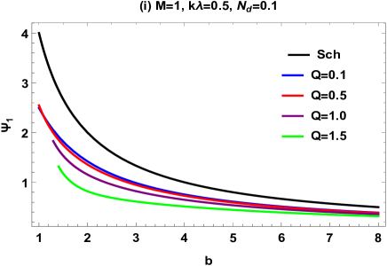
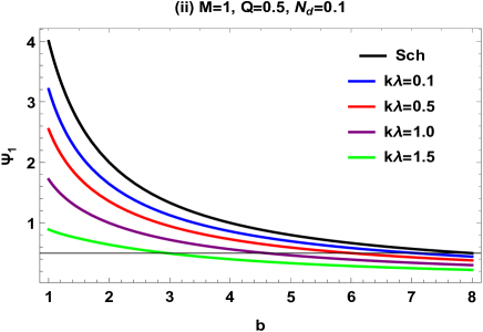
Figure 1: Deflection angle $\psi_{1}$ versus impact parameter $b$ with variations of charge $Q$ and Rastall parameters $k\lambda$ with fixed mass $M=1$ and dust field structure parameter $N_{d}=0.1$

.

In Fig. 1: the left panel shows the variations of charge $Q$ with fixed mass $M=1$, Rastall parameters $k\lambda=0.5$ and dust field structure parameter $N_{d}=0.1$ and right panel represents the variations of Rastall parameters $k\lambda$ with fixed mass $M=1$, charge $Q=0.5$ and dust field structure parameter $N_{d}=0.1$. In both panels the black curve gives the Schwarzschild solution. We can observe that the DA for rising values of charge and Rastall parameters from a BH surrounded by a dust field is decreasing via rising impact parameter and it attains an asymptotically flat form till $b\rightarrow\infty$. A strong deflection can be observed for small value of impact parameter $b=1.2$. Graphically, we can also see the inverse relationship between impact parameter $b$ and DA $\psi_{1}$.

III.1 BLACK HOLE SURROUNDED BY THE QUINTESSENCE FIELD

The metric functions for a BH surrounded by a quintessence field are given as

$$A(r)=\frac{1}{B(r)}=1-\frac{2M}{r}+\frac{Q^{2}}{r^{2}}-\frac{N_{q}}{r^{\frac{-1-2k\lambda}{1-k\lambda}}}~{}~{}C(r)=r^{2},~{}~{}D(r)=r^{2}\sin^{2}\theta.$$ (45)

Using Eqs. (31) and (32), the Gaussian curvature for a BH surrounded by a quintessence field can be defined as

$$K\approx\frac{2M}{r^{3}}+\frac{4Q^{2}N_{q}}{r^{3}}+\frac{18Q^{2}k\lambda N_{q}}{4r^{3}}-\frac{3Q^{2}}{r^{4}}+\frac{6MQ^{2}}{r^{5}}+O(M^{2},Q^{4},\lambda^{2}).$$ (46)

The $\sqrt{\det\vec{g}}$ for the corresponding BH can be calculated as

$$\sqrt{\det\vec{g}}=\frac{3M}{r^{2}}+\frac{1}{r^{3}}-\frac{3Q^{2}}{2r^{3}}+\frac{3N_{q}}{2r^{1+\frac{-1-2k\lambda}{1-k\lambda}}}.$$ (47)

Using Eqs. (46) and (47) into Eq. (42), we obtain the DA for BH surrounded by quintessence field as follows

$$\psi_{2}\approx\frac{4M}{b}+\frac{8N_{q}Q^{2}}{b}+\frac{9N_{q}Q^{2}k\lambda}{b}-\frac{3Q^{2}\pi}{4b^{2}}+\frac{8MQ^{2}}{3b^{3}}+O(M^{2},Q^{4},\lambda^{2}).$$ (48)

The DA in non-plasma medium for a BH surrounded by a quintessence field depends on impact parameter $b$, BH mass $M$, charge $Q$, Rastall geometric parameters $k$, $\lambda$ and quintessential field structure parameter $N_{q}$. Furthermore, it is important to note that the above result reduces to the DA of Reissner–Nordström BH in the absence of the structure parameter $N_{q}=0$ and the Rastall parameters $k\lambda=0$. In addition, we recover the DA of Schwarzschild BH $\psi_{Sch}=4M/b$ in the absence of charge $Q=0$.

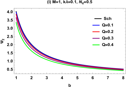
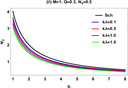
Figure 2: Deflection angle $\psi_{2}$ via impact parameter $b$ with variations of charge $Q$ and Rastall parameters $k\lambda$ with fixed mass $M=1$ and quintessential field structure parameter $N_{q}=0.5$.

In Fig. 2: the left panel displays variations in charge $Q$ with fixed mass $M=1$, Rastall parameters $k\lambda=0.1$, and quintessential field structure parameter $N_{q}=0.5$, whereas Rastall parameters $k\lambda$ with fixed mass $M=1$, charge $Q=0.3$, and quintessential field structure parameter $N_{q}=0.5$ are represented in the right panel. In both panels, the Schwarzschild solution is indicated by the black curve. From a BH surrounded by a quintessential field, we can see that the DA for rising values of charge and Rastall parameters is decreasing via rising impact parameter, reaching an asymptotically flat form till $b\rightarrow\infty$. A significant deflection is seen for small value of impact parameter. Additionally, the inverse relationship between impact parameter $b$ and DA $\psi_{2}$ is also observed.

III.2 BLACK HOLE SURROUNDED BY THE RADIATION FIELD

The metric function for a BH surrounded by a radiation field is defined as

$$A(r)=\frac{1}{B(r)}=1-\frac{2M}{r}+\frac{Q^{2}-N_{r}}{r^{2}},~{}~{}~{}~{}~{}~{}C(r)=r^{2},~{}~{}~{}~{}~{}~{}D(r)=r^{2}\sin^{2}\theta.$$ (49)

Utilizing Eqs. (31) and (32), the Gaussian curvature for a BH surrounded by the radiation field can be computed as follows

$$K\approx\frac{2M}{r^{3}}-\frac{3Q^{2}}{r^{4}}+\frac{3N_{r}}{r^{4}}+\frac{6MQ^{2}}{r^{5}}-\frac{6MN_{r}}{r^{5}}+\frac{4N_{r}Q^{2}}{r^{6}}+O(M^{2},Q^{4}).$$ (50)

The value of $\sqrt{\det\vec{g}}$ for associated BH is given by

$$\sqrt{\det\vec{g}}=\frac{3M}{r^{2}}+\frac{1}{r^{3}}-\frac{3Q^{2}}{2r^{3}}+\frac{3N_{r}}{2r^{3}}.$$ (51)

Using Eqs. (50) and (51) into Eq. (42), we derive the DA for BH surrounded by radiation field as

$$\psi_{3}\approx\frac{4M}{b}-\frac{3Q^{2}\pi}{4b^{2}}+\frac{3N_{r}\pi}{4b^{2}}+\frac{8MQ^{2}}{3b^{3}}-\frac{8MN_{r}}{3b^{3}}+\frac{3N_{r}Q^{2}\pi}{8b^{4}}+O(M^{2},Q^{4}).$$ (52)

The DA in non-plasma frame for a BH surrounded by a radiation field is dependent on impact parameter $b$, BH mass $M$, charge $Q$ and radiation field structure parameter $N_{r}$. It is important to note that the above result reduces to the DA of Reissner–Nordström BH in the absence of the structure parameter $N_{r}=0$. In addition, we recover the DA of Schwarzschild BH $\psi_{Sch}=4M/b$ in the absence of charge $Q=0$.

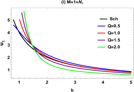
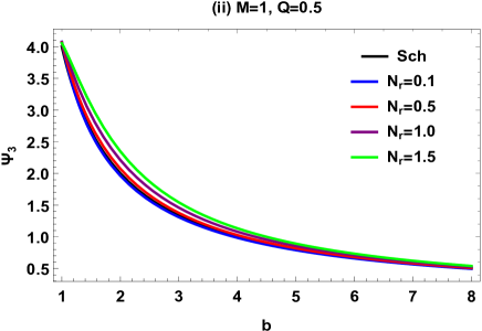
Figure 3: Deflection angle $\psi_{3}$ with respect to impact parameter $b$ with variations of charge $Q$ and radiation field structure parameter $N_{r}$ with fixed mass $M=1$.

Fig. 3: in the left panel charge $Q$ varied with fixed mass and the radiation field structure parameter $M=1=N_{r}$, while the right panel shows variations of radiation field structure parameter $N_{r}$ with fixed mass $M=1$ and charge $Q=0.5$. The black curve in both panels indicates the Schwarzschild solution. The DA with increasing charge and structure parameter values is diminishing by growing impact parameter from a BH surrounded by a radiation field, achieving an asymptotically flat form till $b\rightarrow\infty$. A notable deviation is observed when the impact parameter is minimal. Furthermore, the impact parameter $b$ and DA $\psi_{3}$ are found to be inversely related. It is important to mention here that, at some points in left plot the light deflects with the same angle for different variations of charge. Moreover, a strong deflection can be observed in the presence of radiation field as compared to Schwarzschild case.

III.3 BLACK HOLE SURROUNDED BY THE PHANTOM FILED

The metric functions for a BH surrounded by a phantom field are given by

$$A(r)=\frac{1}{B(r)}=1-\frac{2M}{r}+\frac{Q^{2}}{r^{2}}-\frac{N_{p}}{r^{\frac{-3+2k\lambda}{1+k\lambda}}},~{}~{}~{}~{}~{}C(r)=r^{2},~{}~{}~{}~{}~{}D(r)=r^{2}\sin^{2}\theta.$$ (53)

Considering Eqs. (31) and (32), the Gaussian curvature for a BH surrounded by the phantom field can be given as follows

$$K\approx\frac{2M}{r^{3}}+\frac{4k\lambda M}{r^{3}}-\frac{3Q^{2}}{r^{4}}-\frac{35N_{p}k\lambda Q^{2}}{2r^{4}}+\frac{6MQ^{2}}{r^{5}}-\frac{11N_{p}M}{r^{5}}+O(M^{2},Q^{4},\lambda^{2}).$$ (54)

The $\sqrt{\det\vec{g}}$ for given BH is computed as

$$\sqrt{\det\vec{g}}=\frac{3M}{r^{2}}+\frac{1}{r^{3}}-\frac{3Q^{2}}{2r^{3}}+\frac{3N_{p}}{2r^{1+\frac{-3+2k\lambda}{1+k\lambda}}}.$$ (55)

Utilizing Eqs. (54) and (55) into Eq. (42), we derive the DA for BH surrounded by phantom field as follows

$$\psi_{4}\approx\frac{4M}{b}+\frac{8Mk\lambda}{b}-\frac{35N_{p}k\lambda Q^{2}\pi}{8b^{2}}-\frac{3Q^{2}\pi}{4b^{2}}+\frac{8MQ^{2}}{3b^{3}}-\frac{44N_{p}M}{9b^{3}}+O(M^{2},Q^{4},\lambda^{2}).$$ (56)

The DA in non-plasma medium for a BH surrounded by a phantom field depends on impact parameter $b$, BH mass $M$, charge $Q$, Rastall geometric parameters $k$, $\lambda$ and phantom field structure parameter $N_{p}$. It is significant to note that in the absence of the structure parameter $N_{p}=0$ and the Rastall parameters $k\lambda=0$, the above result simplifies to the DA of Reissner–Nordström BH. Furthermore, in the absence of charge $Q=0$, we recover the DA of Schwarzschild BH $\psi_{Sch}=4M/b$.

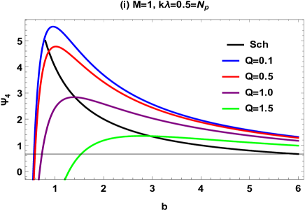
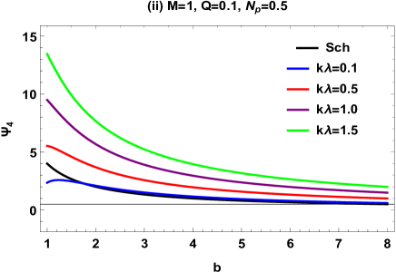
Figure 4: Deflection angle $\psi_{4}$ versus impact parameter $b$ with variations of charge $Q$ and Rastall parameters $k\lambda$ with fixed mass $M=1$ and phantom field structure parameter $N_{p}=0.5$.

Fig. 4: in the left panel charge $Q$ shows variations with fixed mass, Rastall parameters and the phantom field structure parameter $k\lambda=0.5=N_{p}$, while the right panel represents the variations of Rastall parameters $k\lambda$ with fixed mass $M=1$, charge $Q=0.1$ and phantom field structure parameter $N_{p}=0.5$. The Schwarzschild solution is shown by the black curve in both images. As the charge and Rastall parameters values increase, the DA decreases due to an increasing impact parameter from a BH encircled by a phantom field. A strong deflection is shown when the impact parameter is small. Moreover, an inverse relationship between the impact parameter $b$ and the DA $\psi_{4}$ is discovered. It is significant to note that, for various variations in charge, the light deflects at certain spots in the left plot with the same angle for Schwarzschild. Furthermore, a significant deviation from the Schwarzschild scenario can be seen when a phantom field is present.

III.4 BLACK HOLE SURROUNDED BY THE COSMOLOGICAL CONSTANT

The metric functions for a BH surrounded by a cosmological constant is defined as

$$A(r)=\frac{1}{B(r)}=1-\frac{2M}{r}+\frac{Q^{2}}{r^{2}}-N_{c}r^{2},~{}~{}~{}~{}~{}C(r)=r^{2},~{}~{}~{}~{}~{}D=r^{2}\sin^{2}\theta.$$ (57)

Considering Eqs. (31) and (32), the Gaussian curvature for a BH surrounded by the cosmological constant is computed as

$$K\approx\frac{2M}{r^{3}}+\frac{N_{c}}{r^{3}}-\frac{3Q^{2}}{r^{4}}-\frac{6MN_{c}}{r^{4}}+\frac{6MQ^{2}}{r^{5}}+\frac{6N_{c}Q^{2}}{r^{5}}+O(M^{2},Q^{4}).$$ (58)

The value of $\sqrt{\det\vec{g}}$ for BH surrounded by cosmological constant is calculated in the following way

$$\sqrt{\det\vec{g}}=\frac{3M}{r^{2}}+\frac{1}{r^{3}}-\frac{3Q^{2}}{2r^{3}}+\frac{3rN_{c}}{2}.$$ (59)

Utilizing Eqs. (58) and (59) into Eq. (42), we investigate the DA for BH surrounded by cosmological constant as follows

$$\psi_{5}\approx\frac{4M}{b}+\frac{2N_{c}}{b}-\frac{3MN_{c}\pi}{2b^{2}}-\frac{3Q^{2}\pi}{4b^{2}}+\frac{8N_{c}Q^{2}}{3b^{3}}+\frac{8MQ^{2}}{3b^{3}}+O(M^{2},Q^{4}).$$ (60)

The DA in non-plasma medium for a BH surrounded by a cosmological constant depends upon impact parameter $b$, BH mass $M$, charge $Q$ and cosmological field structure parameter $N_{c}$. The above conclusion simplifies to the DA of Reissner-Nordström BH in the absence of the structure parameter $N_{c}=0$. Furthermore, we obtain the DA of Schwarzschild BH $\psi_{Sch}=4M/b$, in the absence of charge $Q=0$.

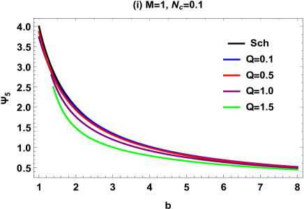
Figure 5: Deflection angle $\psi_{5}$ via impact parameter $b$ with variations of charge $Q$ and cosmological field structure parameter $N_{c}$ with fixed mass $M=1$.

Fig. 5: in the left panel charge $Q$ varied with fixed mass and the radiation field structure parameter $N_{c}=0.1$, while the right panel gives variations of cosmological field structure parameter $N_{c}$ with fixed mass $M=1$ and charge $Q=0.5$.

The Schwarzschild solution is shown in both panels by the black curve. As the impact parameter grows from a BH surrounded by cosmological field, the DA decreases with increasing charge and structure parameter values, reaching an asymptotically flat form until $b\rightarrow\infty$. When the impact parameter is small, a strong deflection is seen. In addition, an inverse relationship is established between the impact parameter $b$ and the DA $\psi_{5}$. It should be noted that, for varying charges, the light deflects at certain spots in the right plot at the same angle as compared to the Schwarzschild case, a significant deflection is shown in the presence of cosmological field.

IV DEFLECTION ANGLE IN THE CONTEXT OF PLASMA MEDIUM

This section studies the computation of the DA in the context of plasma medium. Plasma is another important component that influences a gravitational lens R58 ; Tsupko:2021yca . Refraction in plasma causes increased deflection. The refractive index attempts to obtain auxiliary components and is especially important in the radio regime. Consider $v$ be the velocity of light as it travels through hot, ionised gas to understand the impacts of plasma. The refractive index, $n(r)=c/v$ for a BH surrounded by dust field is given by R41 .

$$n(r)=\sqrt{1-\frac{\omega^{2}_{e}}{\omega^{2}_{\infty}}A(r)},$$ (61)

where $c=1$ as well as $\omega^{2}_{\infty}$ is the photon frequency measured by an observer at infinity and $\omega^{2}_{e}$ is the electron plasma frequency. The optical metric in terms of plasma medium can be defined as

$$d\sigma^{2}=g^{opt}_{ij}dx^{i}dx^{j}=n^{2}\left(\frac{B(r)}{A(r)}dr^{2}+\frac{r^{2}}{A(r)}d\phi^{2}\right).$$ (62)

The optical Gaussian curvature for a BH surrounded by dust field in terms of plasma frame can be calculated as follows

$$K \approx \frac{2M}{r^{3}}+\frac{(1+6k\lambda)N_{d}}{r^{3}}+\frac{12kM\lambda}{r^{3}}-\frac{3Q^{2}}{r^{4}}+\frac{3(2k\lambda-1)MN_{d}}{r^{4}}+\frac{6MQ^{2}}{r^{5}}+\frac{3(2-\lambda)N_{d}Q^{2}}{2r^{5}}+\frac{6M\omega^{2}_{e}}{r^{3}\omega^{2}_{\infty}}+\frac{3N_{d}\omega^{2}_{e}}{r^{3}\omega^{2}_{\infty}}$$ (63)

$$- \frac{15\lambda kN_{d}\omega^{2}_{e}}{2r^{3}\omega^{2}_{\infty}}-\frac{12MN_{d}\omega^{2}_{e}}{r^{4}\omega^{2}_{\infty}}-\frac{5Q^{2}\omega^{2}_{e}}{r^{4}\omega^{2}_{\infty}}+\frac{30kM\lambda N_{d}\omega^{2}_{e}}{r^{4}\omega^{2}_{\infty}}+\frac{13N_{d}Q^{2}\omega^{2}_{e}}{r^{5}\omega^{2}_{\infty}}+\frac{26Q^{2}M\omega^{2}_{e}}{r^{5}\omega^{2}_{\infty}}-\frac{15\lambda kN_{d}Q^{2}\omega^{2}_{e}}{r^{5}\omega^{2}_{\infty}}$$

$$+ O(M^{2},Q^{3},\lambda^{2},\omega^{4}_{e}).$$

Using the GBT, we calculate the bending angle. To do this, we use the straight line approximation $e=\frac{b}{\sin\phi}$ at zeroth order, and the DA is obtained as

$$\psi_{1}\approx-\int^{\pi}_{0}\int^{\infty}_{b/\sin\phi}K\sqrt{det\vec{g}}drd\phi.$$ (64)

The DA of the BH surrounded by dust field in terms of plasma frame for the leading order terms is computed as

$$\psi_{1} \approx \frac{4M}{b}-\frac{2N_{d}}{b}-\frac{12N_{d}k\lambda}{b}+\frac{24Mk\lambda}{b}-\frac{3Q^{2}\pi}{4b^{2}}-\frac{3MN_{d}\pi}{2b^{2}}-\frac{3MN_{d}k\lambda\pi}{2b^{2}}-\frac{4NQ^{2}}{3b^{3}}+\frac{8MQ^{2}}{3b^{3}}+\frac{2N_{d}Q^{2}k\lambda}{3b^{3}}+\frac{6M\omega^{2}_{e}}{b\omega^{2}_{\infty}}$$ (65)

$$+ \frac{6N_{d}\omega^{2}_{e}}{b\omega^{2}_{\infty}}-\frac{15N_{d}k\lambda\omega^{2}_{e}}{b\omega^{2}_{\infty}}-\frac{5Q^{2}\pi\lambda\omega^{2}_{e}}{4b^{2}\omega^{2}_{\infty}}+\frac{15MN_{d}k\lambda\omega^{2}_{e}}{2b^{2}\omega^{2}_{\infty}}-\frac{21MN_{d}\pi\omega^{2}_{e}}{4b^{2}\omega^{2}_{\infty}}+\frac{52N_{d}Q^{2}\omega^{2}_{e}}{9b^{3}\omega^{2}_{\infty}}+\frac{104MQ^{2}\omega^{2}_{e}}{9b^{3}\omega^{2}_{\infty}}-\frac{20N_{d}Q^{2}k\lambda\omega^{2}_{e}}{3b^{3}\omega^{2}_{\infty}}$$

$$+ O(M^{2},Q^{4},\lambda^{2},\omega^{4}_{e}).$$

The DA for a BH surrounded by a dust field depends on impact parameter $b$, BH mass $M$, charge $Q$, Rastall geometric parameters $k$ and $\lambda$, field structure parameters $N_{d}$ as well as plasma frequencies $\omega_{\infty}$ & $\omega_{e}$. Moreover, it is important to mention here that, when, we ignore the plasma effects in Eq. (65) such that $\omega^{2}_{e}/\omega^{2}_{\infty}\rightarrow 0$, then, we recover the results of Eq. (44) in a non-plasma medium.

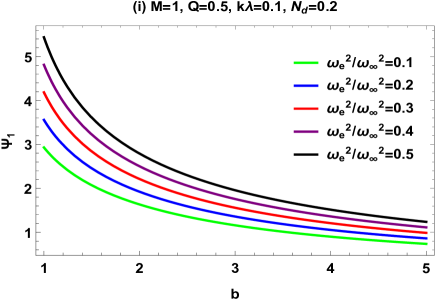
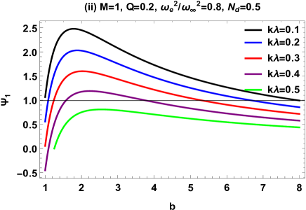
Figure 6: Deflection angle $\psi_{1}$ w.r.t impact parameter $b$ with variations of ratio of plasma frequencies $\omega^{2}_{e}/\omega^{2}_{\infty}$ and Rastall parameters $k\lambda$ with fixed mass $M=1$.

In Fig. 6: the left panel shows the variations of ratio of plasma frequencies $\omega^{2}_{e}/\omega^{2}_{\infty}$ with fixed mass $M=1$, charge $Q=0.2$, Rastall parameters $k\lambda=0.1$ and dust field structure parameter $N_{d}=0.2$ and right panel represents the variations of Rastall parameters $k\lambda$ with fixed mass $M=1$, charge $Q=0.2$, ratio of plasma frequencies $\omega^{2}_{e}/\omega^{2}_{\infty}=0.8$ and dust field structure parameter $N_{d}=0.5$. It is evident that when the impact parameter rises, the DA for increasing plasma frequencies and Rastall parameters from a BH encircled by a dust field decreases. A significant inclination is observable at low impact parameter values where we observe the strongest deflection. The inverse link between impact parameter $b$ and DA $\psi_{1}$ is also visually apparent.

IV.1 BLACK HOLE SURROUNDED BY THE QUINTESSENCE FIELD

The Gaussian curvature for a BH surrounded by a quintessence field under the influence of plasma medium can be given as

$$K \approx \frac{2M}{r^{3}}+\frac{4Q^{2}N_{q}}{r^{3}}+\frac{9Q^{2}k\lambda N_{q}}{2r^{3}}-\frac{3Q^{2}}{r^{4}}+\frac{6MQ^{2}}{r^{5}}+\frac{3M\omega^{2}_{e}}{r^{3}\omega^{2}_{\infty}}+\frac{9N_{q}k\lambda Q^{2}\omega^{2}_{e}}{r^{3}\omega^{2}_{\infty}}+\frac{11N_{q}Q^{2}\omega^{2}_{e}}{r^{3}\omega^{2}_{\infty}}-\frac{5Q^{2}\omega^{2}_{e}}{r^{4}\omega^{2}_{\infty}}+\frac{26MQ^{2}\omega^{2}_{e}}{r^{5}\omega^{2}_{\infty}}$$ (66)

$$+ O(M^{2},Q^{4},\lambda^{2},\omega^{4}_{e}).$$

The DA of a BH surrounded by the quintessence field in a plasma frame for the leading order terms is calculated as

$$\psi_{2} \approx \frac{4M}{b}+\frac{8N_{q}Q^{2}}{b}+\frac{9N_{q}Q^{2}k\lambda}{b}-\frac{3Q^{2}\pi}{4b^{2}}+\frac{8MQ^{2}}{3b^{3}}+\frac{6M\omega^{2}_{e}}{b\omega^{2}_{\infty}}+\frac{22N_{q}Q^{2}\omega^{2}_{e}}{b\omega^{2}_{\infty}}+\frac{18N_{q}k\lambda Q^{2}\omega^{2}_{e}}{b\omega^{2}_{\infty}}-\frac{5Q^{2}\pi\omega^{2}_{e}}{4b^{2}\omega^{2}_{\infty}}$$ (67)

$$+ \frac{104MQ^{2}\omega^{2}_{e}}{9b^{3}\omega^{2}_{\infty}}+O(M^{2},Q^{4},\lambda^{2},\omega^{4}_{e}).$$

The DA in plasma medium for a BH surrounded by a quintessence field depends on impact parameter $b$, BH mass $M$, charge $Q$, Rastall geometric parameters $k$ and $\lambda$, field structure parameters $N_{q}$ as well as plasma frequencies $\omega_{\infty}$ & $\omega_{e}$. It has also worth to note that, when, we ignore the plasma effects in Eq. (67) such that $\omega^{2}_{e}/\omega^{2}_{\infty}\rightarrow 0$, then, we recover the results of Eq. (48) in a non-plasma medium.

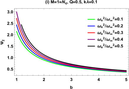
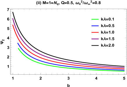
Figure 7: Deflection angle $\psi_{2}$ versus impact parameter $b$ with variations in ratio of plasma frequencies $\omega^{2}_{e}/\omega^{2}_{\infty}$ and Rastall parameters $k\lambda$ with fixed mass, quintessential field structure parameter $M=1=N_{d}$ and charge $Q=0.5$.

In Fig. 7: the left panel displays variations in ratio of plasma frequencies $\omega^{2}_{e}/\omega^{2}_{\infty}$ with fixed mass, quintessential field structure parameter $M=1=N_{d}$, charge $Q=0.5$ and Rastall parameters $k\lambda=0.1$, whereas variations in Rastall parameters $k\lambda$ with with fixed mass, quintessential field structure parameter $M=1=N_{d}$, charge $Q=0.5$ and ratio of plasma frequencies $\omega^{2}_{e}/\omega^{2}_{\infty}=0.8$ are represented in the right panel. The DA for increasing plasma frequencies and Rastall parameter values is shown to decrease via growing impact parameter from a BH surrounded by a quintessential field, eventually achieving an asymptotically flat form until $b\rightarrow\infty$. A notable deviation with strong deflection is observed when the impact parameter is minimal. Furthermore, the inverse link between DA $\psi_{2}$ and impact parameter $b$ is also noted.

IV.2 BLACK HOLE SURROUNDED BY THE RADIATION FIELD

The Gaussian curvature for the BH metric surrounded by a radiation field in the presence of plasma can be calculated as follows

$$K \approx \frac{2M}{r^{3}}-\frac{3Q^{2}}{r^{4}}+\frac{3N_{r}}{r^{4}}+\frac{6MQ^{2}}{r^{5}}-\frac{6MN_{r}}{r^{5}}+\frac{4N_{r}Q^{2}}{r^{6}}+\frac{3M\omega^{2}_{e}}{r^{3}\omega^{2}_{\infty}}-\frac{5Q^{2}\omega^{2}_{e}}{r^{4}\omega^{2}_{\infty}}+\frac{5N_{r}\omega^{2}_{e}}{r^{4}\omega^{2}_{\infty}}+\frac{26MQ^{2}\omega^{2}_{e}}{r^{5}\omega^{2}_{\infty}}-\frac{26MN_{r}\omega^{2}_{e}}{r^{5}\omega^{2}_{\infty}}$$ (68)

$$+ \frac{20Q^{2}N_{r}\omega^{2}_{e}}{r^{6}\omega^{2}_{\infty}}+O(M^{2},Q^{4},\omega^{4}_{e}).$$

The DA of a BH surrounded by the radiation field in a plasma medium can be computed as

$$\psi_{3} \approx \frac{4M}{b}-\frac{3Q^{2}\pi}{4b^{2}}+\frac{3N_{r}\pi}{4b^{2}}+\frac{8MQ^{2}}{3b^{3}}-\frac{8MN_{r}}{3b^{3}}+\frac{3N_{r}Q^{2}\pi}{8b^{4}}+\frac{6M\omega^{2}_{e}}{b\omega^{2}_{\infty}}+\frac{5N_{r}\pi\omega^{2}_{e}}{4b^{2}\omega^{2}_{\infty}}-\frac{5Q^{2}\pi\omega^{2}_{e}}{4b^{2}\omega^{2}_{\infty}}-\frac{104MN_{r}\omega^{2}_{e}}{9b^{3}\omega^{2}_{\infty}}$$ (69)

$$+ \frac{104MQ^{2}\omega^{2}_{e}}{9b^{3}\omega^{2}_{\infty}}+\frac{15NQ^{2}\pi\omega^{2}_{e}}{8b^{4}\omega^{2}_{\infty}}+O(M^{2},Q^{4},\omega^{4}_{e}).$$

The DA in plasma frame for a BH surrounded by a radiation field is dependent on impact parameter $b$, BH mass $M$, charge $Q$, radiation field structure parameter $N_{r}$ as well as plasma frequencies $\omega_{\infty}$ & $\omega_{e}$. It has also worth to mention here that, when, we neglect the plasma effects in Eq. (69) i. e., $\omega^{2}_{e}/\omega^{2}_{\infty}\rightarrow 0$, then, we obtain the results of Eq. (52) in a non-plasma frame.

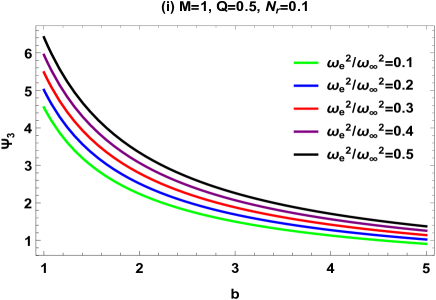
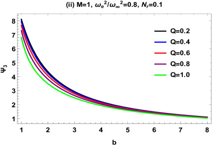
Figure 8: Deflection angle $\psi_{3}$ via impact parameter $b$ with variations of plasma frequencies ratio $\omega^{2}_{e}/\omega^{2}_{\infty}$ and charge $Q$ with fixed mass $M=1$ and radiation field structure parameter $N_{r}$.

Fig. 8: in the left panel charge plasma frequencies ratio $\omega^{2}_{e}/\omega^{2}_{\infty}$ varies with fixed mass and the radiation field structure parameter $M=1$, charge $Q=0.5$ and radiation field structure parameter $N_{r}=0.1$, whereas the right panel shows variations of charge $Q$ with fixed mass $M=1$, plasma frequencies ratio $\omega^{2}_{e}/\omega^{2}_{\infty}=0.8$ and radiation field structure parameter $N_{r}=0.1$. As the impact parameter grows from a BH surrounded by a radiation field, the DA with increasing charge and plasma frequencies ratio diminishes, reaching an asymptotically flat form until $b\rightarrow\infty$. A significant deflection is shown when the impact parameter is small. Moreover, an inverse relationship between the impact parameter $b$ and DA $\psi_{3}$ is discovered. A strong deflection occurs with the increasing ratio of plasma frequencies.

IV.3 BLACK HOLE SURROUNDED BY THE PHANTOM FILED

In the presence of plasma frame, the curvature for a BH surrounded by a phantom field can be computed in the following way

$$K \approx \frac{2M}{r^{3}}+\frac{4k\lambda M}{r^{3}}-\frac{3Q^{2}}{r^{4}}-\frac{35N_{p}k\lambda Q^{2}}{2r^{4}}+\frac{6MQ^{2}}{r^{5}}-\frac{11N_{p}M}{r^{5}}+\frac{3M\omega^{2}_{e}}{r^{3}\omega^{2}_{\infty}}-\frac{4Mk\lambda\omega^{2}_{e}}{r^{3}\omega^{2}_{\infty}}-\frac{5Q^{2}\omega^{2}_{e}}{r^{4}\omega^{2}_{\infty}}-\frac{55N_{p}k\lambda Q^{2}\omega^{2}_{e}}{r^{4}\omega^{2}_{\infty}}$$ (70)

$$- \frac{36MN_{p}\omega^{2}_{e}}{r^{5}\omega^{2}_{\infty}}+\frac{26MQ^{2}\omega^{2}_{e}}{r^{5}\omega^{2}_{\infty}}+O(M^{2},Q^{4},\lambda^{2},\omega^{4}_{e}).$$

The DA in a plasma medium of the BH surrounded by a phantom field is derived as

$$\psi_{4} \approx \frac{4M}{b}+\frac{8Mk\lambda}{b}-\frac{35N_{p}k\lambda Q^{2}\pi}{8b^{2}}-\frac{3Q^{2}\pi}{4b^{2}}+\frac{8MQ^{2}}{3b^{3}}-\frac{44N_{p}M}{9b^{3}}+\frac{6M\omega^{2}_{e}}{b\omega^{2}_{\infty}}-\frac{8Mk\lambda\omega^{2}_{e}}{b\omega^{2}_{\infty}}-\frac{5Q^{2}\pi\omega^{2}_{e}}{4b^{2}\omega^{2}_{\infty}}$$ (71)

$$- \frac{55N_{p}k\lambda Q^{2}\pi\omega^{2}_{e}}{4b^{2}\omega^{2}_{\infty}}-\frac{16N_{p}M\omega^{2}_{e}}{b^{3}\omega^{2}_{\infty}}+\frac{104MQ^{2}\omega^{2}_{e}}{9b^{3}\omega^{2}_{\infty}}+O(M^{2},Q^{4},\lambda^{2},\omega^{4}_{e}).$$

The DA in plasma medium for a BH surrounded by a phantom field depends upon impact parameter $b$, BH mass $M$, charge $Q$, Rastall geometric parameters $k$ and $\lambda$, field structure parameters $N_{p}$ as well as plasma frequencies $\omega_{\infty}$ & $\omega_{e}$. It has important to mention here that, when, we neglect the plasma effects in Eq. (71) i. e., $\omega^{2}_{e}/\omega^{2}_{\infty}\rightarrow 0$, then, we obtain the results of Eq. (56) in a non-plasma medium.

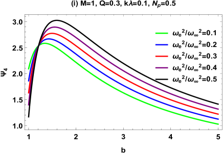
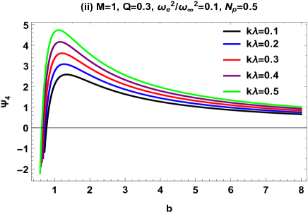
Figure 9: Deflection angle $\psi_{4}$ w.r.t impact parameter $b$ with variations of plasma frequencies ratio $\omega^{2}_{e}/\omega^{2}_{\infty}$ and Rastall parameters $k\lambda$ with fixed mass $M=1$, charge $Q=0.5$ and phantom field structure parameter $N_{p}=0.5$.

Fig. 9: in the left panel charge plasma frequencies ratio $\omega^{2}_{e}/\omega^{2}_{\infty}$ show variations with fixed mass $M=1$, charge $Q=0.3$, Rastall parameters $k\lambda=0.1$ and the phantom field structure parameter $N_{p}=0.5$, while the right panel represents the variations of Rastall parameters $k\lambda$ with fixed mass $M=1$, charge $Q=0.3$, plasma frequencies ratio $\omega^{2}_{e}/\omega^{2}_{\infty}=0.1$ and phantom field structure parameter $N_{p}=0.5$. Due to a rising impact parameter from a BH surrounded by a phantom field, the DA falls as the values of the plasma frequencies ratio and Rastall parameters rise. When the impact parameter is modest, a significant deflection is observed. Furthermore, a negative correlation is seen between the DA $\psi_{4}$ and the impact parameter $b$.

IV.4 BLACK HOLE SURROUNDED BY THE COSMOLOGICAL CONSTANT

In order to calculate the DA for BH surrounded by cosmological constant, we first compute the Gaussian curvature in the following way

$$K \approx \frac{2M}{r^{3}}+\frac{N_{c}}{r^{3}}-\frac{3Q^{2}}{r^{4}}-\frac{6MN_{c}}{r^{4}}+\frac{6N_{c}Q^{2}}{r^{5}}+\frac{6MQ^{2}}{r^{5}}+\frac{3M\omega^{2}_{e}}{r^{3}\omega^{2}_{\infty}}+\frac{3N_{c}\omega^{2}_{e}}{r^{3}\omega^{2}_{\infty}}-\frac{5Q^{2}\omega^{2}_{e}}{r^{4}\omega^{2}_{\infty}}+\frac{16N_{c}Q^{2}\omega^{2}_{e}}{r^{5}\omega^{2}_{\infty}}+\frac{18MN_{c}\omega^{2}_{e}}{r^{4}\omega^{2}_{\infty}}$$ (72)

$$+ \frac{26MQ^{2}\omega^{2}_{e}}{r^{5}\omega^{2}_{\infty}}+O(M^{2},Q^{4},\omega^{4}_{e}).$$

In a plasma frame, the DA of the BH surrounded by the cosmological constant for the leading order terms is calculated as

$$\psi_{5} \approx \frac{4M}{b}+\frac{2N_{c}}{b}-\frac{3MN_{c}\pi}{2b^{2}}-\frac{3Q^{2}\pi}{4b^{2}}+\frac{8N_{c}Q^{2}}{3b^{3}}+\frac{8MQ^{2}}{3b^{3}}+\frac{6M\omega^{2}_{e}}{b\omega^{2}_{\infty}}+\frac{6N_{c}\omega^{2}_{e}}{b\omega^{2}_{\infty}}-\frac{5Q^{2}\pi\omega^{2}_{e}}{4b^{2}\omega^{2}_{\infty}}+\frac{9MN_{c}\pi\omega^{2}_{e}}{2b^{2}\omega^{2}_{\infty}}+\frac{4N_{c}Q^{2}\omega^{2}_{e}}{b^{3}\omega^{2}_{\infty}}$$ (73)

$$+ \frac{104MQ^{2}\omega^{2}_{e}}{9b^{3}\omega^{2}_{\infty}}+O(M^{2},Q^{4},\omega^{4}_{e}).$$

The DA in plasma medium for a BH surrounded by a cosmological constant depends upon impact parameter $b$, BH mass $M$, charge $Q$, cosmological field structure parameter $N_{c}$ as well as plasma frequencies $\omega_{e}$ & $\omega_{\infty}$. It has also worth to mention here that, when, we neglect the plasma effects in Eq. (73) i. e., $\omega^{2}_{e}/\omega^{2}_{\infty}\rightarrow 0$, then, we get the results of Eq. (60) in a non-plasma frame.

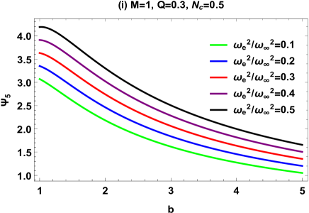
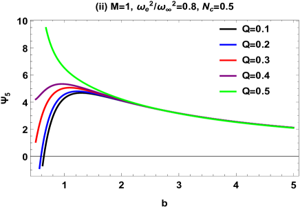
Figure 10: Deflection angle $\psi_{5}$ via impact parameter $b$ with variations of plasma frequencies ratio $\omega^{2}_{e}/\omega^{2}_{\infty}$ and charge $Q$ with fixed mass $M=1$ and cosmological field structure parameter $N_{c}=0.5$.

Fig. 10: in the left panel plasma frequencies ratio varies with fixed mass $M=1$, charge $Q=0.3$ and the radiation field structure parameter $N_{c}=0.5$, while the right panel gives variations of charge $Q$ with fixed mass $M=1$, cosmological field structure parameter $N_{c}=0.5$ and plasma frequencies ratio $\omega^{2}_{e}/\omega^{2}_{\infty}=0.8$.

The DA reduces with increasing plasma frequencies ratio and charge, achieving an asymptotically flat form until $b\rightarrow\infty$. This drop occurs as the impact parameter grows from a BH surrounded by cosmological field. There is a significant strong deflection observed when the impact parameter is modest. Furthermore, a negative correlation is seen between the DA $\psi_{5}$ and the impact parameter $b$.

V EQUATIONS OF MOTION FOR LIGHT RAYS IN A NON-MAGNETIZED PLASMA

This study examines the shadow cast by a BH surrounded by a dust field given in Eq. (22) and the impact of Rastall parameters on it. The core of the critical curve, also known as the apparent boundary, is represented by a BH shadow. This curve has been optimised so that light rays that are a part of it approach a bound orbit of photons asymptotically when a distant observer follows them back to the BH Perlick:2021aok ; R58 .

For a photon, the Hamilton-Jacobi method in the equatorial plane $\theta=\frac{\pi}{2}$ is given as

$$H=\frac{1}{2}\left(g^{ik}j_{i}j_{k}+\omega_{p}(r^{2})\right)=\frac{1}{2}\left(-\frac{y^{2}_{t}}{A(r)}+\frac{y^{2}_{r}}{B(r)}+\frac{y^{2}_{\phi}}{D(r)}+\omega_{p}(r^{2})\right),$$ (74)

where $j_{i}$ represents the momentum of the photon, $y_{\phi}=j_{\phi}$ is its angular momentum and $y_{t}=-j_{t}$ is the photon’s energy. The light rays are the solutions to Hamilton’s equations for a derivation of the Hamiltonian Eq. (74) from Maxwell’s equations with a two-fluid source as

$$\dot{y_{i}}=-\frac{\partial H}{\partial x^{i}},~{}~{}~{}~{}~{}~{}~{}~{}~{}\dot{x^{i}}=-\frac{\partial H}{\partial y_{i}}.$$ (75)

The above equations implies

$$\dot{y_{t}} = -\frac{\partial H}{\partial t}=0,~{}~{}~{}~{}~{}~{}~{}~{}~{}~{}\dot{y_{\phi}}=-\frac{\partial H}{\partial\psi}=0,$$ (76)

$$\dot{y_{r}} = -\frac{\partial H}{\partial r}=\frac{1}{2}\left(-\frac{y^{2}_{t}A^{\prime}(r)}{A(r)^{2}}+\frac{y^{2}_{r}B^{\prime}(r)}{B(r)^{2}}+\frac{y^{2}_{\phi}D^{\prime}(r)}{D(r)^{2}}-\frac{d}{dr}\omega_{p}(r^{2})\right),$$ (77)

$$\dot{t} = \frac{\partial H}{\partial y_{t}}=-\frac{y_{t}}{A(r)},$$ (78)

$$\dot{\phi} = \frac{\partial H}{\partial y_{\phi}}=-y_{\phi},$$ (79)

$$\dot{r} = \frac{\partial H}{\partial y_{r}}=-\frac{y_{r}}{B(r)}.$$ (80)

In this case, a prime denotes differentiation with regard to $r$, while a dot denotes differentiation with respect to an affine parameter $\lambda$.

By setting $H=0$ in Eq. (74), we get the result in this form

$$0=-\frac{y^{2}_{t}}{A(r)}+\frac{y^{2}_{r}}{B(r)}+\frac{y^{2}_{\phi}}{D(r)}+\omega_{p}(r^{2}).$$ (81)

From Eq. (76), it is followed that the $y_{t}$ and $y_{\phi}$ are constants of motion. We consider $\omega_{0}=-j_{t}$. Given a fixed $\omega_{0}$ and an asymptotically flat spacetime (e.g., $A(r)\rightarrow 1$ as $r\rightarrow\infty$), the gravitational redshift formula transforms the frequency $\omega$ as measured by a static observer into a function of $r$ in the given form

$$\omega(r)=\frac{\omega_{0}}{\sqrt{A(r)}}.$$ (82)

As a result of Eq. (81), a light beam with constant speed $\omega_{0}$ is limited to the area where

$$\frac{\omega^{2}_{0}}{A(r)}>\omega_{p}(r)^{2}.$$ (83)

The constraint (82) states that the photon frequency $\omega(r)$ must exceed the plasma frequency $\omega_{p}(r)$ at a given place. For light to propagate through a plasma, this is always true. In order to obtain the orbit equation, we use Eq. (78) and Eq. (79) and get

$$\frac{dr}{d\phi}=\frac{\dot{r}}{\dot{\phi}}=\frac{D(r)y_{r}}{B(r)y_{\phi}}.$$ (84)

Using $y_{r}$ from Eq. (81), we get the result in this form

$$\frac{dr}{d\phi}=\pm\frac{\sqrt{D(r)}}{\sqrt{B(r)}}\sqrt{\frac{\omega^{2}_{0}v(r)^{2}}{y^{2}_{\phi}}-1},$$ (85)

where

$$v(r)^{2}=\frac{D(r)}{A(r)}\left(1-A(r)\frac{\omega_{p}^{2}}{\omega_{0}^{2}}\right).$$ (86)

Since $X$ is the turning point of the trajectory, the condition $\frac{dr}{d\phi}\Big{|}_{X}=0$ must hold. This equation connects $X$ to the constant of motion, $\frac{y_{\phi}}{\omega_{0}}$ as follows

$$v(X)^{2}=\frac{y_{\psi}^{2}}{\omega_{0}^{2}}.$$ (87)

The shadow’s radius is defined by the original direction of the photon’s light, which is asymptotically radial towards the outer photon sphere. In order to calculate the shadow of the BH surrounded by a dust field, we consider a light beam projected with an angle $\gamma$ in the radial direction from the observer point $r_{0}$. We define $\gamma$ in the following way

$$\cot\gamma=\pm\frac{\sqrt{g_{rr}}}{\sqrt{g_{\phi\phi}}}\frac{dr}{d\phi}\Big{|}_{r=r_{0}}=\pm\frac{\sqrt{B(r)}}{\sqrt{D(r)}}\frac{dr}{d\phi}\Big{|}_{r=r_{0}}.$$ (88)

We rewrite the orbit equation Eq. (85) after attaining a minimum radius $R$ by using Eq. (87) in the form

$$\frac{dr}{d\phi}=\pm\frac{\sqrt{D(r)}}{\sqrt{B(r)}}\sqrt{\frac{v(r_{0})^{2}}{v(X)^{2}}-1}.$$ (89)

Using Eq. (89) into Eq. (88) for the angle $\gamma$, we get

$$\cot^{2}\gamma={\frac{v(r_{0})^{2}}{v(X)^{2}}-1}.$$ (90)

By using the identity, we obtain

$$1+\cot^{2}\gamma=\frac{1}{\sin^{2}\gamma}.$$ (91)

Using Eq. (91) into (90), we get the result

$$\sin^{2}\gamma=\frac{v(X)^{2}}{v(r_{0})^{2}}.$$ (92)

Light rays spiralling asymptotically towards a circular light orbit at radius $r_{ph}$ define the boundary of the shadow $\gamma$. Consequently, $X\rightarrow r_{ph}$ in Eq. (92) provides the angular radius of the shadow as

$$\sin^{2}\gamma=\frac{v(r_{ph})^{2}}{v(r_{0})^{2}},$$ (93)

where $v(r_{0})$ can be represented by the formula in Eq. (85) at $r=r_{0}$. In numerous cases, it is possible to presume that the observer is situated in an area with a negligible plasma density. Then Eq. (85) implies

$$v(r_{0})^{2}=\frac{D(r_{0})}{A(r_{0})},$$ (94)

and Eq. (93) can be written as follows

$$\sin^{2}\gamma=\frac{A(r_{0})D(r_{ph})}{A(r_{ph})D(r_{0})}\left(1-\frac{A(r_{ph})\omega_{p}^{2}(r_{ph})}{\omega^{2}_{o}}\right).$$ (95)

After substituting the values of metric function into the above equation, we obtain the result into following manner

$$\sin^{2}\gamma=\frac{r^{2}_{ph}\left(2Mr_{0}-Q^{2}-r^{2}_{0}+N_{d}r^{\frac{1}{1-3k\lambda}}_{0}\right)\left(Q^{2}\omega^{2}_{p}-2Mr_{ph}\omega^{2}_{p}+r^{2}_{ph}(\omega^{2}_{P}-\omega^{2}_{0})-N_{d}r^{\frac{1}{1-3k\lambda}}_{ph}\omega^{2}_{p}\right)}{r^{4}_{0}\left(Q^{2}-2Mr_{ph}+r^{2}_{ph}-N_{d}r^{\frac{1}{1-3k\lambda}}_{ph}\right)\omega^{2}_{0}}.$$ (96)

The shadow of the BH surrounded by a dust field is dependent on BH mass $M$, charge $Q$, Rastall parameters $k,~{}\lambda$, dust field structure parameter $N_{d}$, plasma frequencies $\omega_{p},~{}\omega_{0}$, photon radius $r_{ph}$ and observer radius $r_{0}$.

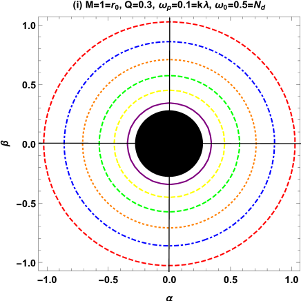
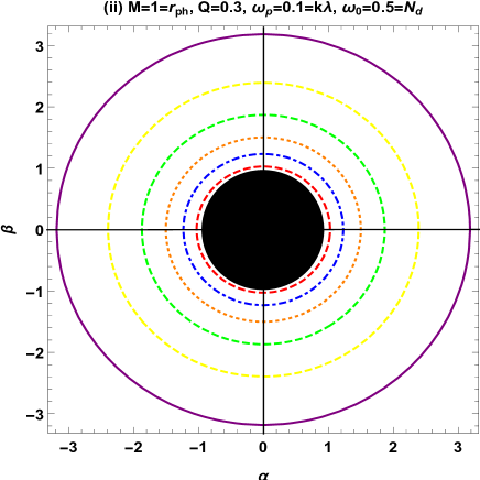
Figure 11: Shadow of BH surrounded by dust field in celestial plane $(\alpha,\beta)$ for variations of photon radius $r_{ph}$ and observer radius $r_{0}$.

Fig. 11: the left panel shows the contour plots of shadow for variations of photon radius $r_{ph}=0.5$ (purple), $0.6$ (yellow), $0.7$ (green), $0.8$ (orange), $0.9$ (blue) and $1$ (red) with fixed values of mass $M=1$, observer radius $r_{0}=1$, charge $Q=0.3$, plasma frequencies $\omega_{p}=0.1,~{}\omega_{0}=0.5$, Rastall parameters $k\lambda=0.1$ and dust field structure parameter $N_{d}=0.5$. One can see that when the photon radius rises, the shadow radius size also increases.

The right panel gives the contour plots of shadow for different choices of radius $r_{0}=0.5$ (purple), $0.6$ (yellow), $0.7$ (green), $0.8$ (orange), $0.9$ (blue), $1$ (red) and fixed mass $M=1$, charge $Q=0.3$, photon radius $r_{ph}=1$, plasma frequencies $\omega_{p}=0.1,~{}\omega_{0}=0.5$, Rastall parameters $k\lambda=0.1$ and dust field structure parameter $N_{d}=0.5$. It can be observed that the size of shadow radius decreases with increasing observers radius $r_{0}$ and it is bigger than photon radius.

V.1 BLACK HOLE SURROUNDED BY THE QUINTESSENCE FIELD

After putting the values of metric function from Eq. (45) into Eq. (95), we get the result in the given form

$$\sin^{2}\gamma_{1}=\frac{r^{2}_{ph}\left(2Mr_{0}-Q^{2}-r^{2}_{0}+N_{q}r^{1+\frac{3k\lambda}{-1+k\lambda}}_{0}\right)\left(Q^{2}\omega^{2}_{p}-2Mr_{ph}\omega^{2}_{p}+r^{2}_{ph}(\omega^{2}_{P}-\omega^{2}_{0})-N_{q}r^{1+\frac{3k\lambda}{-1+k\lambda}}_{ph}\omega^{2}_{p}\right)}{r^{4}_{0}\left(Q^{2}-2Mr_{ph}+r^{2}_{ph}-N_{q}r^{1+\frac{3k\lambda}{-1+k\lambda}}_{ph}\right)\omega^{2}_{0}}.$$ (97)

The shadow of the BH surrounded by a quintessence field is dependent on BH mass $M$, charge $Q$, Rastall parameters $k,~{}\lambda$, quintessence field structure parameter $N_{q}$, plasma frequencies $\omega_{p},~{}\omega_{0}$, photon radius $r_{ph}$ and observer radius $r_{0}$.

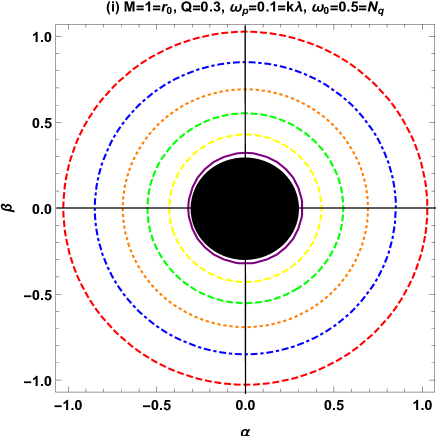
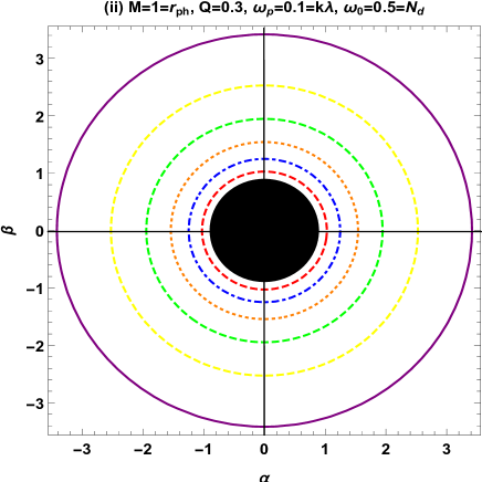
Figure 12: Shadow of BH surrounded by quintessential field in celestial plane $(\alpha,\beta)$ for variations of photon radius $r_{ph}$ and observer radius $r_{0}$.

Fig. 12: the left panel represents the contour plots of shadow for variations of photon radius $r_{ph}=0.5$ (purple), $0.6$ (yellow), $0.7$ (green), $0.8$ (orange), $0.9$ (blue) and $1$ (red) with fixed values of mass $M=1$, observer radius $r_{0}=1$, charge $Q=0.3$, plasma frequencies $\omega_{p}=0.1,~{}\omega_{0}=0.5$, Rastall parameters $k\lambda=0.1$ and dust field structure parameter $N_{q}=0.5$. We can observe that when the photon radius rises, the shadow radius size also increases.

The right panel gives the contour plots of shadow for different choices of radius $r_{0}=0.5$ (purple), $0.6$ (yellow), $0.7$ (green), $0.8$ (orange), $0.9$ (blue), $1$ (red) and fixed mass $M=1$, charge $Q=0.3$, photon radius $r_{ph}=1$, plasma frequencies $\omega_{p}=0.1,~{}\omega_{0}=0.5$, Rastall parameters $k\lambda=0.1$ and dust field structure parameter $N_{q}=0.5$. It can be observed that the size of shadow radius decreases with increasing observers radius $r_{0}$.

V.2 BLACK HOLE SURROUNDED BY THE RADIATION FIELD

After substituting the values of metric function from Eq. (49) into Eq. (95), we obtain the result in the given form

$$\sin^{2}\gamma_{2}=\frac{r^{2}_{ph}\left(2Mr_{0}-Q^{2}-r^{2}_{0}+N_{r}\right)\left(Q^{2}\omega^{2}_{p}-2Mr_{ph}\omega^{2}_{p}+r^{2}_{ph}(\omega^{2}_{P}-\omega^{2}_{0})-N_{r}\omega^{2}_{p}\right)}{r^{4}_{0}\left(Q^{2}-2Mr_{ph}+r^{2}_{ph}-N_{r}\right)\omega^{2}_{0}}.$$ (98)

The shadow of the BH surrounded by a phantom field depends upon BH mass $M$, charge $Q$, radiation field structure parameter $N_{r}$, plasma frequencies $\omega_{p},~{}\omega_{0}$, photon radius $r_{ph}$ and observer radius $r_{0}$.

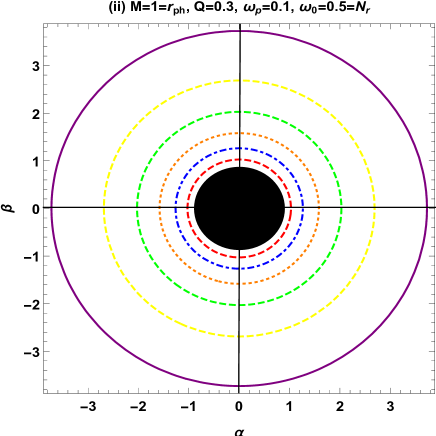
Figure 13: Shadow of BH surrounded by radiation field in celestial plane $(\alpha,\beta)$ for variations of photon radius $r_{ph}$ and observer radius $r_{0}$.

Fig. 13: the left panel illustrate the contour plots of shadow for variations of photon radius $r_{ph}=0.5$ (purple), $0.6$ (yellow), $0.7$ (green), $0.8$ (orange), $0.9$ (blue) and $1$ (red) with fixed values of mass $M=1$, observer radius $r_{0}=1$, charge $Q=0.3$, plasma frequencies $\omega_{p}=0.1,~{}\omega_{0}=0.5$, Rastall parameters $k\lambda=0.1$ and dust field structure parameter $N_{r}=0.5$. We can see that the shadow radius size increases along with the photon radius.

The right panel gives the contour plots of shadow for different choices of radius $r_{0}=0.5$ (purple), $0.6$ (yellow), $0.7$ (green), $0.8$ (orange), $0.9$ (blue), $1$ (red) and fixed mass $M=1$, charge $Q=0.3$, photon radius $r_{ph}=1$, plasma frequencies $\omega_{p}=0.1,~{}\omega_{0}=0.5$, Rastall parameters $k\lambda=0.1$ and dust field structure parameter $N_{r}=0.5$. It is shown that when the observers radius $r_{0}$ increases, the shadow radius’s size reduces.

V.3 BLACK HOLE SURROUNDED BY THE PHANTOM FILED

After putting the values of metric function from Eq. (53) into Eq. (95), we get the result as follows

$$\sin^{2}\gamma_{3}=\frac{r^{2}_{ph}\left(2Mr_{0}-Q^{2}-r^{2}_{0}+N_{p}r^{\frac{5}{1+k\lambda}}_{0}\right)\left(Q^{2}\omega^{2}_{p}-2Mr_{ph}\omega^{2}_{p}+r^{2}_{ph}(\omega^{2}_{P}-\omega^{2}_{0})-N_{p}r^{\frac{5}{1+k\lambda}}_{ph}\omega^{2}_{p}\right)}{r^{4}_{0}\left(Q^{2}-2Mr_{ph}+r^{2}_{ph}-N_{p}r^{\frac{5}{1+k\lambda}}_{ph}\right)\omega^{2}_{0}}.$$ (99)

The shadow of the BH surrounded by a phantom field depends on BH mass $M$, charge $Q$, Rastall parameters $k,~{}\lambda$, phantom field structure parameter $N_{p}$, plasma frequencies $\omega_{p},~{}\omega_{0}$, photon radius $r_{ph}$ and observer radius $r_{0}$.

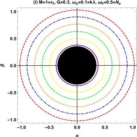
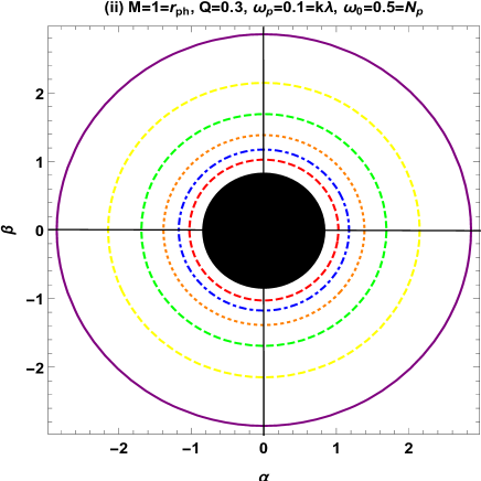
Figure 14: Shadow of BH surrounded by phantom field in celestial plane $(\alpha,\beta)$ for variations of photon radius $r_{ph}$ and observer radius $r_{0}$.

Fig. 14: the left panel depicts the contour plots of shadow for different choices of photon radius $r_{ph}=0.5$ (purple), $0.6$ (yellow), $0.7$ (green), $0.8$ (orange), $0.9$ (blue) and $1$ (red) with fixed values of mass $M=1$, observer radius $r_{0}=1$, charge $Q=0.3$, plasma frequencies $\omega_{p}=0.1,~{}\omega_{0}=0.5$, Rastall parameters $k\lambda=0.1$ and dust field structure parameter $N_{p}=0.5$. It is evident that as the photon radius rises, so does the shadow radius size.

The right panel shows the contour plots of shadow for variations of radius $r_{0}=0.5$ (purple), $0.6$ (yellow), $0.7$ (green), $0.8$ (orange), $0.9$ (blue), $1$ (red) and fixed mass $M=1$, charge $Q=0.3$, photon radius $r_{ph}=1$, plasma frequencies $\omega_{p}=0.1,~{}\omega_{0}=0.5$, Rastall parameters $k\lambda=0.1$ and dust field structure parameter $N_{p}=0.5$. It is demonstrated that the size of the shadow radius decreases with increasing observers radius $r_{0}$.

V.4 BLACK HOLE SURROUNDED BY THE COSMOLOGICAL CONSTANT

After using the values of metric function from Eq. (57) into Eq. (95), we acquire the result in the given form

$$\sin^{2}\gamma_{4}=\frac{r^{2}_{ph}\left(2Mr_{0}-Q^{2}-r^{2}_{0}+N_{c}r^{4}_{0}\right)\left(Q^{2}\omega^{2}_{p}-2Mr_{ph}\omega^{2}_{p}+r^{2}_{ph}(\omega^{2}_{P}-\omega^{2}_{0})-N_{c}r^{4}_{ph}\omega^{2}_{p}\right)}{r^{4}_{0}\left(Q^{2}-2Mr_{ph}+r^{2}_{ph}-N_{c}r^{4}_{ph}\right)\omega^{2}_{0}}.$$ (100)

The shadow of the BH surrounded by a cosmological constant depends on BH mass $M$, charge $Q$, cosmological field structure parameter $N_{c}$, plasma frequencies $\omega_{p},~{}\omega_{0}$, photon radius $r_{ph}$ and observer radius $r_{0}$.

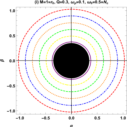
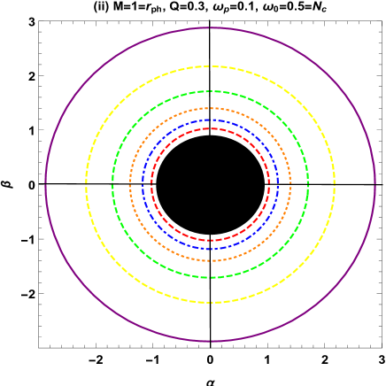
Figure 15: Shadow of BH surrounded by cosmological field in celestial plane $(\alpha,\beta)$ for variations of photon radius $r_{ph}$ and observer radius $r_{0}$.

Fig. 15: the left panel represents the contour plots of shadow for different choices of photon radius $r_{ph}=0.5$ (purple), $0.6$ (yellow), $0.7$ (green), $0.8$ (orange), $0.9$ (blue) and $1$ (red) with fixed values of mass $M=1$, observer radius $r_{0}=1$, charge $Q=0.3$, plasma frequencies $\omega_{p}=0.1,~{}\omega_{0}=0.5$, Rastall parameters $k\lambda=0.1$ and dust field structure parameter $N_{c}=0.5$. It is clear that the shadow radius size increases with the photon radius.

The right panel shows the contour plots of shadow for variations of radius $r_{0}=0.5$ (purple), $0.6$ (yellow), $0.7$ (green), $0.8$ (orange), $0.9$ (blue), $1$ (red) and fixed mass $M=1$, charge $Q=0.3$, photon radius $r_{ph}=1$, plasma frequencies $\omega_{p}=0.1,~{}\omega_{0}=0.5$, Rastall parameters $k\lambda=0.1$ and dust field structure parameter $N_{c}=0.5$. It is shown that as the observers radius $r_{0}$ increases, the shadow radius’s size decreases.

VI Conclusions

In the framework of Rastall theory, we have studied generic charged BH solutions surrounded by an ideal fluid. Next, we have looked more closely into the particular situations of BHs encircled by dust, quintessence, radiation, phantom fields and cosmological constant. In the generalized theory, physical parameters are studied by applying the weak energy condition, which signifies a positive energy density. An effective behaviour of the BH surrounding the field is realized by comparing the solution in GR with the new term in the metric that arose from the Rastall theory. The ray tracing and generalized GW methods offer a comprehensive Rastall framework for characterizing strategies for the Kiselev BH solution. In the non-plasma, plasma and perfect fluid mediums, we have talked about the Rastall solution and derived DA by using the GW technique. The Gaussian optical curvature is determined for this purpose using an optical metric and we have then examined the DA using GBT.

Firstly, we investigated the DA for BHs surrounded by dust, quintessence, radiation, phantom and cosmological fields in a non-plasma medium. We have concluded from our results that BHs surrounded by dust, quintessence and phantom fields are dependent on impact parameter $b$, BH mass $M$, charge $Q$, Rastall geometric parameters $k$, $\lambda$ and field structure parameters $N_{d},~{}N_{q}$ and $N_{p}$, respectively. Moreover, the DA for BHs surrounded by radiation field and cosmological constant depends upon on impact parameter $b$, BH mass $M$, charge $Q$ and field structure parameters $N_{r}$ and $N_{c}$, respectively. We also observed analytically and graphically that the impact parameter $b$ is in an inverse relation with the DA of corresponding BHs. Moreover, it has worth to mention here that, in the absence of structure and Rastall parameters, the results of DA of our corresponding BHs reduce into DA of Reissner–Nordström BH as well as in the absence of charge $Q=0$, we recovered the DA of Schwarzschild BH $\psi_{Sch}=4M/b$.

With the help of graphical interpretation, we showed that the impact parameter $b$ has an inverse relation with DA. Moreover, by comparing the graphical conduct of DA of our corresponding BHs with Schwarzschild case, we concluded that BHs surrounded by dust, quintessence fields and cosmological constants have less deflection as compared to Schwarzschild BH. In addition, we observed strong deflection is seen for small value of impact parameter in all plots of non-plasma medium.

Secondly, we examined the DA for BHs surrounded by dust, quintessence, radiation, phantom and cosmological fields in a plasma medium and concluded that the DA for BHs surrounded by dust, quintessence and phantom fields depends upon impact parameter $b$, BH mass $M$, charge $Q$, Rastall geometric parameters $k$ and $\lambda$, as well as plasma frequencies $\omega_{\infty}$ & $\omega_{e}$ and field structure parameters $N_{d},~{}N_{q}$ and $N_{p}$, respectively. Moreover, the DA for BHs surrounded by radiation field and cosmological constant depends upon on impact parameter $b$, BH mass $M$, charge $Q$, plasma frequencies $\omega_{\infty}$ & $\omega_{e}$ and field structure parameters $N_{r}$ and $N_{c}$, respectively. It has important to mention here that, when, we neglect the plasma effects in our results i. e., $\omega^{2}_{e}/\omega^{2}_{\infty}\rightarrow 0$, then, we obtained the results of DA in a non-plasma medium for corresponding BHs.

After that, we analyzed the graphical results for DA in the presence of plasma for variations of plasma frequencies ratio $\omega^{2}_{e}/\omega^{2}_{\infty}$, Rasatll parameters $k\lambda$ and charge $Q$. Furthermore, from our graphical analysis, we concluded that the DA for increasing plasma frequencies and Rastall parameter values is shown to decrease via growing impact parameter from a BH surrounded by a dust, quintessential and phantom field that eventually achieving an asymptotically flat form until $b\rightarrow\infty$. A notable deviation with strong deflection is observed when the impact parameter is minimal. Furthermore, the inverse link between DA and impact parameter $b$ is also noted in the presence of plasma medium.

At last, we investigated the shadows of BHs defined by the Kiselev solution in the Rastall theory. A Hamiltonian equation that is variable-separable and a light-ray motion equation are independent of the plasma’s velocity in the presence of a pressure-less and non-magnetized plasma. We explored the perfect fluid in Rastall theory, where particle accumulation is correlated with the plasma frequency. The scenario in which plasma falls radially upon a BH from infinity is investigated in terms of dust, quintessence, radiation, phantom fields and cosmological constants encircled by a Rastall solution. Moreover, the shadow of our corresponding BHs depends on BH mass $M$, charge $Q$, Rastall parameters $k,~{}\lambda$, plasma frequencies $\omega_{p},~{}\omega_{0}$, photon radius $r_{ph}$, observer radius $r_{0}$ and their field structure parameters $N_{d},~{}N_{q},~{}N_{r},~{}N_{p}$ and $N_{c}$, respectively. We plotted the contour plots for corresponding BHs for their shadows with variations of photon radius $r_{ph}$ as well as observer radius $r_{0}$. We concluded that the size of shadow radius increases with the rise in photon radius whereas the size of shadow decreases with rise in values of observer’s radius.

The presence of the conical singularity on the symmetric axis in the background of Rastall spacetime is responsible for the appearance of the BHs encircled by phantom fields, quintessence, cosmological constants, radiation, and dust. Examining how a conical singularity affects the DA and shadow variables is interesting. Future reports on this work will be provided.

References

- (1) C. M. Will, The confrontation between general relativity and experiment, Living reviews in relativity 17 (2014) 1.
- (2) S. Weinberg, Principles and Applications of the General Theory of Relativity: Gravitation and Cosmology, Wiley (1972).
- (3) A. Vilenkin, Cosmic strings as gravitational lenses, The Astrophysical Journal 282 (1984) L51.
- (4) A. Vilenkin, Cosmic strings and domain walls, Physics reports 121 (1985) 263.
- (5) J.R. Gott III, Gravitational lensing effects of vacuum strings-exact solutions, The Astrophysical Journal 288 (1985) 422.
- (6) V. Bozza, Gravitational lensing in the strong field limit, Physical Review D 66 (2002) 103001.
- (7) O. Wucknitz and U. Sperhake, Deflection of light and particles by moving gravitational lenses, Physical Review D 69 (2004) 063001.
- (8) W. Rindler and M. Ishak, Contribution of the cosmological constant to the relativistic bending of light revisited, Physical Review D 76 (2007) 043006.
- (9) J. Sultana, Contribution of the cosmological constant to the bending of light in kerr–de sitter spacetime, Physical Review D 88 (2013) 042003.
- (10) A. Bhattacharya, R. Isaev, M. Scalia, C. Cattani and K.K. Nandi, Light bending in the galactic halo by rindler-ishak method, Journal of Cosmology and Astroparticle Physics 2010 (2010) 004.
- (11) A. Bhattacharya, G.M. Garipova, E. Laserra, A. Bhadra and K.K. Nandi, The vacuole model: new terms in the second order deflection of light, Journal of Cosmology and Astroparticle Physics 2011 (2011) 028.
- (12) C. Cattani, M. Scalia, E. Laserra, I. Bochicchio and K.K. Nandi, Correct light deflection in weyl conformal gravity, Physical Review D 87 (2013) 047503.
- (13) A. Mishra and S. Chakraborty, On the trajectories of null and timelike geodesics in different wormhole geometries, The European Physical Journal C 78 (2018) 1.
- (14) M. Ishak, Light deflection, lensing, and time delays from gravitational potentials and fermat’s principle in the presence of a cosmological constant, Physical Review D 78 (2008) 103006.
- (15) M. Sereno, Influence of the cosmological constant on gravitational lensing in small systems, Physical Review D 77 (2008) 043004.
- (16) E. Gallo and O.M. Moreschi, Gravitational lens optical scalars in terms of energy-momentum distributions, Physical Review D 83 (2011) 083007.
- (17) V. Bozza and A. Postiglione, Alternatives to schwarzschild in the weak field limit of general relativity, Journal of Cosmology and Astroparticle Physics 2015 (2015) 036.
- (18) E.F. Boero and O.M. Moreschi, Gravitational lens optical scalars in terms of energy–momentum distributions in the cosmological framework, Monthly Notices of the Royal Astronomical Society 475 (2018) 4683.
- (19) G. Crisnejo and E. Gallo, Expressions for optical scalars and deflection angle at second order in terms of curvature scalars, Physical Review D 97 (2018) 084010.
- (20) D. Glavan and C. Lin, Einstein-gauss-bonnet gravity in four-dimensional spacetime, Physical Review letters 124 (2020) 081301.
- (21) R. Kumar, S.U. Islam and S.G. Ghosh, Gravitational lensing by charged black hole in regularized 4d einstein–gauss–bonnet gravity, The European Physical Journal C 80 (2020) 1.
- (22) K. S. Virbhadra and G. F. R. Ellis, Schwarzschild black hole lensing, Physical Review D 62, 084003 (2000).
- (23) K. S. Virbhadra and G. F. R. Ellis, Gravitational lensing by naked singularities, Physical Review D 65, 103004 (2002).
- (24) K. S. Virbhadra, Relativistic images of Schwarzschild black hole lensing, Physical Review D 79, 083004 (2009).
- (25) G. Lambiase, R. C. Pantig, D. J. Gogoi and A. Övgün, Investigating the connection between generalized uncertainty principle and asymptotically safe gravity in black hole signatures through shadow and quasinormal modes, The European Physical Journal C 83, no.7, 679 (2023).
- (26) K. S. Virbhadra, Distortions of images of Schwarzschild lensing, Physical Review D 106, no.6, 064038 (2022).
- (27) J. R. Nascimento, A. Y. Petrov, P. J. Porfirio and A. R. Soares, Gravitational lensing in black-bounce spacetimes, Physical Review D 102, no.4, 044021 (2020).
- (28) X. M. Kuang and A. Övgün, Strong gravitational lensing and shadow constraint from M87* of slowly rotating Kerr-like black hole, Annals of Physics 447, 169147 (2022).
- (29) X. M. Kuang, Z. Y. Tang, B. Wang and A. Wang, Constraining a modified gravity theory in strong gravitational lensing and black hole shadow observations, Physical Review D 106, no.6, 064012 (2022).
- (30) C. Furtado, J. R. Nascimento, A. Y. Petrov, P. J. Porfírio and A. R. Soares, Strong gravitational lensing in a spacetime with topological charge within the Eddington-inspired Born-Infeld gravity, Physical Review D 103, no.4, 044047 (2021).
- (31) Y. Kumaran and A. Övgün, Deflection Angle and Shadow of the Reissner–Nordström Black Hole with Higher-Order Magnetic Correction in Einstein-Nonlinear-Maxwell Fields, Symmetry 14 (2022) 2054.
- (32) K. Jafarzade, M.K. Zangeneh and F.S. Lobo, Shadow, deflection angle and quasinormal modes of born-infeld charged black holes, Journal of Cosmology and Astroparticle Physics 2021 (2021) 008.
- (33) F. W. Dyson, A.S. Eddington and C. Davidson, Ix. a determination of the deflection of light by the sun’s gravitational field, from observations made at the total eclipse of may 29, 1919, Philosophical Transactions of the Royal Society of London, Series A 220 (1920) 291.
- (34) S. Dodelson, Gravitational lensing, Cambridge University Press (2017).
- (35) B.R. Patla, R.J. Nemiroff, D.H. Hoffmann and K. Zioutas, Flux enhancement of slow-moving particles by sun or jupiter: can they be detected on earth?, The Astrophysical Journal 780 (2013) 158.
- (36) J. Liu and M.S. Madhavacheril, Constraining neutrino mass with the tomographic weak lensing one-point probability distribution function and power spectrum, Physical Review D 99 (2019) 083508.
- (37) A. Accioly and R. Paszko, Photon mass and gravitational deflection, Physical Review D 69 (2004) 107501.
- (38) A. Bhadra, K. Sarkar and K. Nandi, Testing gravity at the second post-newtonian level through gravitational deflection of massive particles, Physical Review D 75 (2007) 123004.
- (39) O.Y. Tsupko, Unbound motion of massive particles in the schwarzschild metric: Analytical description in case of strong deflection, Physical Review D 89 (2014) 084075.
- (40) X. Liu, N. Yang and J. Jia, Gravitational lensing of massive particles in schwarzschild gravity, Classical and Quantum Gravity 33 (2016) 175014.
- (41) G. He and W. Lin, Gravitational deflection of light and massive particles by a moving kerr–newman black hole, Classical and Quantum Gravity 33 (2016) 095007.
- (42) G. He and W. Lin, Analytical derivation of second-order deflection in the equatorial plane of a radially moving kerr–newman black hole, Classical and Quantum Gravity 34 (2017) 105006.
- (43) X. Pang and J. Jia, Gravitational lensing of massive particles in reissner–nordstrom black hole spacetime, Classical and Quantum Gravity 36 (2019) 065012.
- (44) Z. H. Li, X. Zhou, W. J. Li and G. S. He, Gravitational deflection of massive particles by a schwarzschild black hole in radiation gauge, Communications in Theoretical Physics 71 (2019) 1219.
- (45) X. He, T. Xu, Y. Yu, A. Karamat, R. Babar, R. Ali, Deflection angle evolution with plasma medium and without plasma medium in a parameterized black hole. Ann. Phys. 451 (2023) 169247.
- (46) X. He, S. Zhu, Y. Yu, A. Karamat, R. Babar, R. Ali, Deflection angle analysis under the influence of non-plasma medium and plasma medium for regular black hole with cosmic string. Int. J. Geom. Methods Mod. Phys. 20, 2350205(2023).
- (47) G. Gibbons and M. Werner, Applications of the gauss–bonnet theorem to gravitational lensing, Classical and Quantum Gravity 25 (2008) 235009.
- (48) M. Werner, Gravitational lensing in the kerr-randers optical geometry, General Relativity and Gravitation 44 (2012) 3047.
- (49) A. Ishihara, Y. Suzuki, T. Ono, T. Kitamura and H. Asada, Gravitational bending angle of light for finite distance and the gauss-bonnet theorem, Physical Review D 94 (2016) 084015.
- (50) T. Ono, A. Ishihara and H. Asada, Gravitomagnetic bending angle of light with finite-distance corrections in stationary axisymmetric spacetimes, Physical Review D 96 (2017) 104037.
- (51) G. Crisnejo and E. Gallo, Weak lensing in a plasma medium and gravitational deflection of massive particles using the gauss-bonnet theorem. a unified treatment, Physical Review D 97 (2018) 124016.
- (52) Z. Li and J. Jia, The finite-distance gravitational deflection of massive particles in stationary spacetime: a jacobi metric approach, The European Physical Journal C 80 (2020) 1.
- (53) R. Ali, M. Awais and A. Mahmood, Study of the Deflection Angle and Shadow of Black Hole Solutions in Non-Plasma and Plasma Mediums Under the Effect of Einstein-Gauss-Bonnet Gravity, Annalen der Physik 535 (2023) 2300236.
- (54) Event Horizon Telescope Collaboration, Akiyama, K., Alberdi, A., et al. 2019a, The Astrophysical Journal Letters, 875, L2.
- (55) J. L. Synge, The Escape of Photons from Gravitationally Intense Stars, Monthly Notices of the Royal Astronomical Society 131 (1966) 463.
- (56) P. V. P. Cunha, C. A. R. Herdeiro and E. Radu, Fundamental photon orbits: black hole shadows and spacetime instabilities, Physical Review D 96 (2017) 024039.
- (57) M. Wang, S. Chen and J. Jing, Shadow casted by a Konoplya-Zhidenko rotating non-Kerr black hole, Journal of Cosmology and Astroparticle Physics 10 (2017) 051.
- (58) Z. Li and C. Bambi, Measuring the Kerr spin parameter of regular black holes from their shadow, Journal of Cosmology and Astroparticle Physics 1401 (2014) 041.
- (59) K. Hioki and K. I. Maeda, Measurement of the Kerr Spin Parameter by Observation of a Compact Object’s Shadow, Physical Review D 80 (2009) 024042.
- (60) R. A. Konoplya, Shadow of a black hole surrounded by dark matter, Physics Letters B 795 (2019) 1.
- (61) X. Hou, Z. Xu, M. Zhou and J. Wang, Black Hole Shadow of SgrA in Dark Matter Halo, Journal of Cosmology and Astroparticle Physics 07 (2018) 015.
- (62) L. Amarilla, E. F. Eiroa, and G. Giribet, Null geodesics and shadow of a rotating black hole in extended Chern-Simons modified gravity, Physical Review D 81 (2010) 124045.
- (63) F. Long, S. Chen, M. Wang, and J.Jing, Shadow of a disformal Kerr black hole in quadratic DHOST theories, The European Physical Journal C 80 (2020) 1180.
- (64) H. C. D. L. Junior, P. V. P. Cunha, C. A. R. Herdeiro and L. C. B. Crispino, Shadows and lensing of black holes immersed in strong magnetic fields, Physical Review D 104 (2021) 044018.
- (65) M. Wang, S. Chen, J. Jing, Kerr Black hole shadows in Melvin magnetic field with stable photon orbits, Physical Review D 104 (2021) 084021.
- (66) V. Perlick, O. Y. Tsupko, and G. S. Bisnovatyi-Kogan, Influence of a plasma on the shadow of a spherically symmetric black hole, Physical Review D 92 (2015) 104031.
- (67) S. Chen, M. Wang, J. Jing, Polarization effects in Kerr black hole shadow due to the coupling between photon and bumblebee field, Journal of High Energy Physics 07 (2020) 054.
- (68) A. Grenzebach, V. Perlick, and C. Lammerzahl, Photon Regions and Shadows of Kerr-NewmanNUT Black Holes with a Cosmological Constant, Physical Review D 89 (2014) 124004.
- (69) V. Perlick, O. Y. Tsupko and G. S. BisnovatyiKogan, Black hole shadow in an expanding universe with a cosmological constant, Physical Review D 97 (2018) 104062.
- (70) M. Wang, S. Chen, J. Wang, J. Jing, Shadow of a Schwarzschild black hole surrounded by a Bach-Weyl ring, The European Physical Journal C 80 (2020) 110.
- (71) P. V. P. Cunha, N. A. Eiro, C. A. R. Herdeiro and J. P. S. Lemos, Lensing and shadow of a black hole surrounded by a heavy accretion disk, Journal of Cosmology and Astroparticle Physics 03 (2020) 035.
- (72) M. Wang, S. Chen, J. Wang, J. Jing, Effect of gravitational wave on shadow of a Schwarzschild black hole, The European Physical Journal C 81 (2021) 509.
- (73) P. G. Nedkova, V. Tinchev, and S. S. Yazadjiev, Shadow of a Rotating Traversable Wormhole, Physical Review D 88 (2013) 124019.
- (74) G. Gyulchev, P. Nedkova, V. Tinchev and S. Yazadjiev, On the shadow of rotating traversable wormholes, The European Physical Journal C 78 (2018) 544.
- (75) N. Ortiz, O. Sarbach and T. Zannias, Shadow of a naked singularity, Physical Review D 92 (2015) 044035.
- (76) D. Dey, R. Shaikh, and P. S. Joshi, Shadow of nulllike and timelike naked singularities without photon spheres, Physical Review D 103 (2021) 024015.
- (77) P. V. P. Cunha, C. A. R. Herdeiro, E. Radu and H. F. Runarsson, Shadows of Kerr black holes with scalar hair, Physical Review Letters 115 (2015) 211102.
- (78) F. H. Vincent, E. Gourgoulhon, C. A. R. Herdeiro and E. Radu, Astrophysical imaging of Kerr black holes with scalar hair, Physical Review D 94 (2016) 084045.
- (79) P. V. P. Cunha, J. Grover, C. A. R. Herdeiro, E. Radu, H. Runarsson, and A. Wittig, Chaotic lensing around boson stars and Kerr black holes with scalar hair, Physical Review D 94 (2016) 104023.
- (80) M. Wang, S. Chen, J. Jing, Shadows of Bonnor black dihole by chaotic lensing, Physical Review D 97 (2016) 064029.
- (81) M. Wang, S. Chen, J. Jing, Chaotic shadow of a non-Kerr rotating compact object with quadrupole mass moment, Physical Review D 98 (2016) 104040.
- (82) T. Johannsen, Photon Rings around Kerr and Kerr like Black Holes, The Astrophysical Journal 777 (2013) 170.
- (83) D. Nitta, T. Chiba and N. Sugiyama, Shadows of Multi-Black Holes: Analytic Exploration, Physical Review D 86 (2012) 103001.
- (84) A. F. Zakharov, Constraints on a Tidal Charge of the Supermassive Black Hole in M87* with the EHT Observations in April 2017, Universe 8, no.3, 141 (2022).
- (85) S. Vagnozzi, R. Roy, Y. D. Tsai, L. Visinelli, M. Afrin, A. Allahyari, P. Bambhaniya, D. Dey, S. G. Ghosh and P. S. Joshi, et al. Horizon-scale tests of gravity theories and fundamental physics from the Event Horizon Telescope image of Sagittarius A, Classical and Quantum Gravity 40, no.16, 165007 (2023).
- (86) S. Vagnozzi and L. Visinelli, Hunting for extra dimensions in the shadow of M87*, Physical Review D 100, no.2, 024020 (2019).
- (87) A. Allahyari, M. Khodadi, S. Vagnozzi and D. F. Mota, Magnetically charged black holes from non-linear electrodynamics and the Event Horizon Telescope, Journal of Cosmology and Astroparticle Physics 02, 003 (2020).
- (88) M. Khodadi, A. Allahyari, S. Vagnozzi and D. F. Mota, Black holes with scalar hair in light of the Event Horizon Telescope, Journal of Cosmology and Astroparticle Physics 09, 026 (2020).
- (89) A. Abdujabbarov, M. Amir, B. Ahmedov and S. G. Ghosh, Shadow of rotating regular black holes, Physical Review D 93, no.10, 104004 (2016).
- (90) F. Atamurotov, A. Abdujabbarov and B. Ahmedov, Shadow of rotating non-Kerr black hole, Physical Review D 88, no.6, 064004 (2013).
- (91) M. Afrin, R. Kumar and S. G. Ghosh, Parameter estimation of hairy Kerr black holes from its shadow and constraints from M87*, Monthly Notices of the Royal Astronomical Society 504, 5927-5940 (2021).
- (92) R. Kumar and S. G. Ghosh, “Rotating black holes in Einstein-Gauss-Bonnet gravity and its shadow,” Journal of Cosmology and Astroparticle Physics 07, 053 (2020).
- (93) F. Atamurotov, I. Hussain, G. Mustafa and A. Övgün, Weak deflection angle and shadow cast by the charged-Kiselev black hole with cloud of strings in plasma*, Chinese Physics C 47, no.2, 025102 (2023).
- (94) G. Mustafa, F. Atamurotov, I. Hussain, S. Shaymatov and A. Övgün, Shadows and gravitational weak lensing by the Schwarzschild black hole in the string cloud background with quintessential field*, Chinese Physics C 46, no.12, 125107 (2022).
- (95) A. Uniyal, R. C. Pantig and A. Övgün, “Probing a non-linear electrodynamics black hole with thin accretion disk, shadow, and deflection angle with M87* and Sgr A* from EHT,” Phys. Dark Univ. 40, 101178 (2023).
- (96) R. C. Pantig, L. Mastrototaro, G. Lambiase and A. Övgün, “Shadow, lensing, quasinormal modes, greybody bounds and neutrino propagation by dyonic ModMax black holes,” Eur. Phys. J. C 82, no.12, 1155 (2022).
- (97) R. C. Pantig, A. Övgün and D. Demir, “Testing symmergent gravity through the shadow image and weak field photon deflection by a rotating black hole using the M87∗ and Sgr. results,” Eur. Phys. J. C 83, no.3, 250 (2023).
- (98) R. C. Pantig and A. Övgün, “Black Hole in Quantum Wave Dark Matter,” Fortsch. Phys. 71, no.1, 2200164 (2023).
- (99) B. Puliçe, R. C. Pantig, A. Övgün and D. Demir, “Constraints on charged symmergent black hole from shadow and lensing,” Class. Quant. Grav. 40, no.19, 195003 (2023).
- (100) G. Lambiase, L. Mastrototaro, R. C. Pantig and A. Ovgun, “Probing Schwarzschild-like black holes in metric-affine bumblebee gravity with accretion disk, deflection angle, greybody bounds, and neutrino propagation,” JCAP 12, 026 (2023).
- (101) K. Okabayashi, N. Asaka and K. Nakao, Do black hole shadows merge?, Physical Review D 102 (2020) 044011.
- (102) E. Babichev, V. Dokuchaev and Yu. Eroshenko, Black Hole Mass Decreasing due to Phantom Energy Accretion, Physical Review Letters 93 (2004) 021102.
- (103) V.V. Kiselev, Quintessence and black holes, Classical and Quantum Gravity 20 (2003) 1187.
- (104) B. Majeed, M. Jamil and P. Pradhan, Thermodynamic Relations for Kiselev and Dilaton Black Hole, Advances in High Energy Physics 2015 (2015) 124910.
- (105) R. Ali, Z. Akhtar, K. Bamba and M. U. Khan, Tunneling and thermodynamics evolution of the magnetised Ernst-like black hole, General Relativity and Gravitation 55 (2023) 28.
- (106) M. Jamil, S. Hussain and B. Majeed, Dynamics of particles around a Schwarzschild-like black hole in the presence of quintessence and magnetic field, The European Physical Journal C 75 (2015) 24.
- (107) P. Rastall, Generalization of the Einstein Theory, Physical Review D 6 (1972) 3357.
- (108) P. Rastall, A theory of gravity, Canadian Journal of Physics 54 (1976) 66.
- (109) V. V. Kiselev, Quintessence and black holes, Classical and Quantum Gravity 20 (2003) 1187.
- (110) Y. Heydarzade and F. Darabi, Black hole solutions surrounded by perfect fuid in Rastall theory, Physics Letters B 771 (2017) 365.
- (111) R. Ali, M. Asgher and M. F. Malik, Gravitational analysis of neutral regular black hole in Rastall gravity. Modern Physics Letters A 35, 2050225(2020).
- (112) R. Ali, K. Bamba, S. A. A. Shah and M. J. Saleem, Tunneling Analysis of Kerr-Newman Black Hole-Like Solution in Rastall Theory. International Journal of Modern Physics D 31 (2022) 2250069.
- (113) Y. Huang, Z. Cao and Z. Lu, Generalized Gibbons-Werner method for stationary spacetimes, Journal of Cosmology and Astroparticle Physics 01 (2024) 013.
- (114) W. Javed, S. Riaz, R. C. Pantig and A. Övgün, Weak gravitational lensing in dark matter and plasma mediums for wormhole-like static aether solution. The European Physical Journal C 82 (2022) 1057.
- (115) Y. Guo and Y. G. Miao, Bounce corrections to gravitational lensing, quasinormal spectral stability and gray-body factors of Reissner-Nordström black holes, Physical Review D 106 (2022) 124052.
- (116) W. Javed, M. Atique, R. C. Pantig and A. Övgün, Weak Deflection Angle, Hawking Radiation and Greybody Bound of Reissner-Nordström Black Hole Corrected by Bounce Parameter, Symmetry 15 (2023) 148.
- (117) O. Y. Tsupko, Deflection of light rays by a spherically symmetric black hole in a dispersive medium, Physical Review D 103, no.10, 104019 (2021).
- (118) V. Perlick and O. Y. Tsupko, Calculating black hole shadows: Review of analytical studies, Physics Reports 947, 1-39 (2022).