Abstract

Deep Neural Nets (DNNs) learn latent representations induced by their downstream task, objective function, and other parameters. The quality of the learned representations impacts the DNN’s generalization ability and the coherence of the emerging latent space. The Information Bottleneck (IB) provides a hypothetically optimal framework for data modeling, yet it is often intractable. Recent efforts combined DNNs with the IB by applying VAE-inspired variational methods to approximate bounds on mutual information, resulting in improved robustness to adversarial attacks. This work introduces a new and tighter variational bound for the IB, improving performance of previous IB-inspired DNNs. These advancements strengthen the case for the IB and its variational approximations as a data modeling framework, and provide a simple method to significantly enhance the adversarial robustness of classifier DNNs.

marginparsep has been altered.
topmargin has been altered.
marginparpush has been altered.
The page layout violates the ICML style. Please do not change the page layout, or include packages like geometry, savetrees, or fullpage, which change it for you. We’re not able to reliably undo arbitrary changes to the style. Please remove the offending package(s), or layout-changing commands and try again.

 

Tighter Bounds on the Information Bottleneck with Application to Deep Learning

 

Nir Weingarten ¹ Zohar Yakhini ¹ Moshe Butman ¹ Ran Gilad-Bachrach ²

1 Introduction

In recent years, Deep Neural Networks (DNNs) have gained prominence in various learning tasks, revolutionizing many computational fields with their ability to approximate complex functions. Despite the great achievements, it is still postulated that the current networks are prone to overfit the training data Ying (2019), may be considerably uncalibrated Guo et al. (2017) and are susceptible to adversarial attacks Goodfellow et al. (2015). A question emerges regarding the extraction of an optimal representation for all data points from a restricted set of training examples. Classic information theory provides tools to optimize compression and transmission of data, but it does not provide methods to gauge the relevance of a compressed signal to its downstream task. Methods such as rate-distortion Blahut (1972) regard all information as equal, not taking into account which information is more relevant without constructing complex distortion functions. The Information Bottleneck (IB) Tishby et al. (1999) resolves this limitation by defining mutual information between the learned representation and the downstream task as a universal distortion function. Under this definition, an optimal rate-disotrion ratio can be implicitly computed for a Lagrange multiplier $\beta$, controlling the tradeoff between the desired rate and distortion. However, optimizing over the IB requires mutual information computations, which are tractable in discrete settings and for some specific continuous distributions. Adopting the IB framework for DNNs requires computing mutual information for unknown distributions and has no analytic solution. However, recent work approximated tractable upper bounds for the IB functional in DNN settings using variational approximations. Variational Auto Encoders (VAEs) Kingma & Welling (2014) use stochastic DNNs to approximate intractable distributions, as elaborated in Section 2.3. Similarly to VAEs, Alemi et al. (2017) proposed using stochastic DNNs as variational approximations of latent models, thus making possible the computations of upper bounds for mutual information between the DNN’s input, output and latent representation. A proposed DNN optimization method called Deep Variational Information Bottleneck (VIB) derives an upper bound for the IB objective and minimizes its approximation by fitting some training dataset. Optimizing classifier DNNs with the VIB objective results in a slight decrease in test set accuracy compared to deterministic DNNs, but yields a significant increase in robustness to adversarial attacks.

In this study, we adopt the same information theoretic and variational approach proposed in VIB. The work begins by deriving a new upper bound for the IB functional. We then employ a tractable variational approximation for this bound, named VUB - ’Variational Upper Bound’ and show that it is a tighter bound on the IB objective than VIB. We proceed to show empirical evidence that VUB substantially increases test set accuracy over VIB while providing similar or superior robustness to adversarial attacks across several challenging tasks and different modalities. Finally, we discuss these effects in the context of previous work on the IB and on DNN regularization. The conclusion drawn is that while increasing mutual information between encoding and output does not necessarily improve classification, and while increasing encoding compression does not always enhance regularization Amjad & Geiger (2020), the application of IB approximations as objectives to DNNs empirically improves regularization, suggesting better data modeling. This notion contributes for the adaptation of the IB, and its variational approximations, as an objective for learning tasks and as a theoretic framework to gauge and explain data modeling.

In addition, we demonstrate that VUB can be easily adapted to any classifier DNN, including transformer based NLP classifiers, to substantially increase robustness to adversarial attacks while only slightly decreasing, or in some cases even increasing, test set accuracy.

1.1 Preliminaries

The following literature review and derivations refer to information theory and variational approximations. A preliminary mutual ground and notation is provided.

We denote random variables (RVs) with upper cased letters $X,Y$, and their realizations in lower case $x,y$. Denote discrete Probability Mass Functions (PMFs) with an upper case $P(x)$ and continuous Probability Density Functions (PDFs) with a lower case $p(x)$. Hat notation denotes empirical measurements.

Let $X,Y$ be two observed random variables with unknown distributions $p^{*}(x),p^{*}(y)$ that we aim to model. Assume $X,Y$ are governed by some unknown underlying process with a joint probability distribution $p^{*}(x,y)$. We can attempt to approximate these distributions using a model $p_{\theta}$ with parameters $\theta$ such that for generative tasks $p_{\theta}(x)\approx p^{*}(x)$ and for discriminative tasks $p_{\theta}(y|x)\approx p^{*}(y|x)$, using a dataset $\mathcal{S}=\left\{(x_{1},y_{1}),...,(x_{N},y_{N})\right\}$ to fit our model. One can also assume the existence of an additional unobserved RV $Z\sim p^{*}(z)$ that influences or generates the observed RVs $X,Y$. Since $Z$ is unobserved it is absent from the dataset $\mathcal{S}$ and so cannot be modeled directly. Denote $\int p_{\theta}(x|z)p_{\theta}(z)dz$ the marginal, $p_{\theta}(z)$ the prior as it is not conditioned over any other RV, and $p_{\theta}(z|x)$ the posterior following Bayes’ rule.

When modeling an unobserved variable of an unknown distribution we encounter a problem as the marginal $p_{\theta}(x)=\int p_{\theta}(x,z)dz$ doesn’t have an analytic solution. This intractability can be overcome by choosing some tractable parametric variational distribution $q_{\phi}(z|x)$ to approximate the posterior $p_{\theta}(z|x)$ such that $q_{\phi}(z|x)\approx p_{\theta}(z|x)$, and estimate $p_{\theta}(x,z)$ or $p_{\theta}(x,z|y)$ by fitting the dataset $\mathcal{S}$ Kingma & Welling (2019).

In this work information theoretic functions share the same notation for discrete and continuous settings. For brevity, we will only present the continuous form:

Entropy	$H_{p}(X)=-\int p(x)log\left(p(x)\right)dx$
Cross Entropy	$CE(p,q)=-\int p(x)log\left(q(x)\right)dx$
KL Divergence	$D_{KL}\left(p\big{|}\big{|}q\right)=\int p(x)log\left(\frac{p(x)}{q(x)}\right)dx$
Mutual Information	$I(X;Y)=\int\int p(x,y)log\left(\frac{p(x,y)}{p(x)p(y)}\right)dxdy$

2 Related work

2.1 IB and its analytic solutions

Classic information theory offers rate-distortion Blahut (1972) to mitigate signal loss during compression. Rate being the signal’s compression measured by mutual information between input and output signals, and distortion a chosen task-specific function. The Information Bottleneck (IB) method Tishby et al. (1999) extends rate-distortion by replacing the tailored distortion functions with mutual information between the learned representation and the downstream task. Denote $X$ the source signal, $Z$ its encoding and $Y$ the target signal for some specific task. Assuming a latent variable model that follows the Markov chain $Z\leftrightarrow X\leftrightarrow Y$, we define some positive minimal threshold $D$ for the desired distortion. We seek an optimal encoding $Z:\underset{P(Z|X)}{min}I(X;Z)$ subject to $I(Z;Y)\geq D$. This constrained problem can be implicitly optimized by minimizing the functional $L_{P(Z|X)}=I(Z;X)-\beta I(Z;Y)$, the first term being rate and the second distortion modulated by the Lagrange multiplier $\beta$. The optimal solution is a function of $\beta$ and was named ’the information curve’ as illustrated in Figure 1. The IB can be interpreted as a method to learn a representation that holds just enough information to satisfy a desired task, while discarding all other available information, presumably providing a model with the least possible complexity.

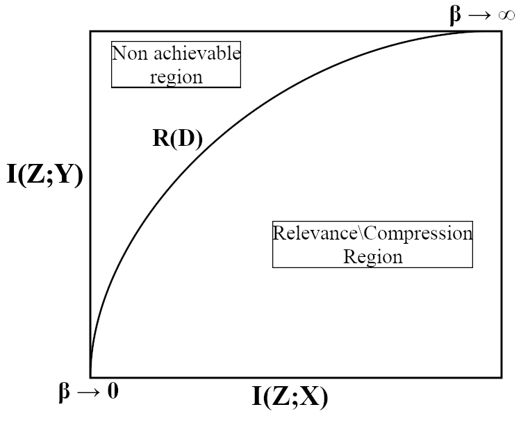
Figure 1: The information plane and curve: rate-distortion ratio over $\beta$. At $\beta=0$ the representation is compressed but uninformative (maximal compression), at $\beta\rightarrow\infty$ the representation is informative but potentially overfitted (maximal information). Adapted from Slonim (2002).

The IB functional is only tractable when mutual information can be computed and was originally demonstrated for soft clustering tasks over a discrete and known distribution $P^{*}(x,y)$. Chechik et al. (2003) extended the IB for gaussian distributions and Painsky & Tishby (2017) offered a limited linear approximation of the IB for any distribution.

2.2 IB and deep learning

Tishby & Zaslavsky (2015) proposed an IB interpretation of DNNs, regarding them as Markov cascades of intermediate representations between hidden layers. Under this framework, comparing the optimal and the achieved rate-distortion ratios between DNN layers will indicate if a model is too complex or too simple for a given task and training set. Shwartz-Ziv & Tishby (2017) visualized and analyzed the information plane behavior of DNNs over a toy problem with a known joint distribution. Mutual information of the different layers was estimated and used to analyze the training process. The learning process over Stochastic Gradient Descent (SGD) exhibited two separate and sequential behaviors: A short Empirical Error Minimization phase (ERM) characterized by a rapid decrease in distortion, followed by a long compression phase with an increase in rate until convergence to an optimal IB limit as demonstrated in Figure 2. Similar yet repetitive behavior was observed in the current study, as elaborated in Section 4.2.1.

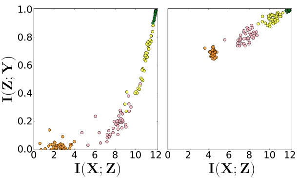
Figure 2: Information plane scatters of different DNN layers (colors) in 50 randomized networks. From Shwartz-Ziv & Tishby (2017). Left are initial weights, Right are at 400 epochs. Our study reproduced similar yet repetitive behavior on complicated high dimensional tasks, as elaborated in Section 4.2.1 and in Figure 3.

Amjad & Geiger (2020) pointed out three flaws in the usage of the IB functional as an objective for deterministic DNN classifiers: (1) When data $X$ is absolutely continuous the mutual information term $I(X;Z)$ is infinite; (2) When data $X$ is discrete the IB functional is a piecewise constant function of the parameters, making it’s SGD optimization difficult or impossible; (3) Equivalent representations might yield the same IB loss while one achieved better classification rate than the other. These discrepancies were attributed to mutual information’s invariance to invertible transformations and to the absence of a decision function in the objective.

2.3 Variational approximations to the IB objective

Kingma & Welling (2014) introduced the Variational Auto Encoder (VAE) - a stochastic generative DNN. An unobserved RV $Z$ is assumed to generate evidence $X$ and the true probability $p^{*}(x)$ can be modeled using a parametric model over the marginal $p_{\theta}(x)=\int p_{\theta}(x|z)p_{\theta}(z)dz$. However, since the marginal is intractable a variational approximation $q_{\phi}(z|x)\approx p_{\theta}(z|x)$ is proposed instead. The log probability $log\left(p_{\theta}(x)\right)$ is then developed in to the tractable VAE loss comprised of the Evidence Lower Bound (ELBO) and KL regularization terms: $\underset{\text{\emph{\text{\emph{ELBO}}}}}{\mathcal{L}}=\mathbb{E}_{q_{\phi}(z|x)}\left[log\left(p_{\theta}(x|z)\right)\right]-D_{KL}\left(q_{\phi}(z|x)\big{|}\big{|}p_{\theta}(z)\right)$. $q_{\phi}(z|x)$ is modeled using a stochastic neural encoder having it’s final activation used as parameters for the assumed variational distribution (typically a spherical gaussian with parameters $\mu,\Sigma$). Each forward pass emulates a stochastic realization $z\in Z$ from these parameters by using the ’reparameterization trick’: $z=\mu+\epsilon\cdot\Sigma$ for some unparameterized scalar $\epsilon\sim N(0,1)$ such that a backwards pass is possible. Higgins et al. (2017) later proposed the $\beta$-autoencoder, introducing a hyper parameter $\beta$ over the KL term to control the regularization-reconstruction tradeoff. Alemi et al. (2018) found that as the ELBO loss in VAEs depends solely on image reconstruction it does not necessarily induce a better quality modeling of the marginal $p_{\theta}(z)$, hence not necessarily a better representation learned. This gap is attributed to powerful decoders being overfitted, as will be further discussed in Section 5.

Alemi et al. (2017) introduced the Variational Information Bottleneck (VIB) as a variational approximation for an upper bound to the IB objective for classifier DNN optimization. Bounds for $I(Z,Y)$ and $I(X,Z)$ are derived from the non negativity of KL divergence and are used to form an upper bound for the IB functional. This upper bound is approximated using variational approximations for $p^{*}(y|z),\,p^{*}(z)$ as done in VAEs. This approximation of an upper bound for the IB objective is empirically estimated as cross entropy and a beta scaled KL regularization term as in $\beta$-autoencoders, and is optimized over the training data using Monte Carlo sampling and the reparameterization trick. VIB was evaluated over image classification tasks and, while causing a slight reduction in test set accuracy, generated substantial improvements in robustness to adversarial attacks.

Additional noteworthy contributions to this field have been made in recent years by Achille & Soatto (2018); Wieczorek & Roth (2019); Fischer (2020) and others. However, a detailed review of these works is beyond the scope of this paper.

2.4 Non IB information theoretic regularization

Label smoothing Szegedy et al. (2016) and entropy regularization Pereyra et al. (2017) both regularize classifier DNNs by increasing the entropy of their output. This is done either directly by inserting a scaled conditional entropy term to the loss function, $-\gamma\cdot H\left(p_{\theta}(y|x)\right)$, or by smoothing the training data labels. Applying both methods was demonstrated to improve test accuracy and model calibration on various challenging classification tasks. In the current work a similar conditional entropy term emerges from the derivation of the new upper bound for the IB objective, as shown in Section 3.

3 From VIB to VUB

The VIB loss consists of a cross entropy term and a KL regularization term, as in VAE loss. The KL term is derived from a bound on the IB rate term $I(X;Z)$, while the cross entropy term from a bound on the IB distortion term $I(Z;Y)=H(Y)-H(Y|Z)$. When deriving the latter the entropy term $H(Y)$ is ignored as it is constant and does not effect optimization. We note that since $Y$ is unknown any optimization over $Z$, including cross entropy, depends on our decoder model of $Y$. Following this logic, instead of omitting $H(Y)$ we replace it with a variational approximation of the decoder entropy, which provides a lower bound.

3.1 IB upper bound

We begin by establishing a new upper bound for the IB functional by bounding the mutual information terms, using the same method as in VIB.

Consider $I(Z;X)$:

$$I(Z;X)= \int\int p^{*}(x,z)log\left(p^{*}(z|x)\right)dxdz$$

$$- \int p^{*}(z)log\left(p^{*}(z)\right)dz$$ (1)

For any probability distribution $r$ we have that $D_{KL}\left(p^{*}(z)\big{|}\big{|}r(z)\right)\geq 0$, it follows that:

$$\int p^{*}(z)log\left(p^{*}(z)\right)dz\geq\int p^{*}(z)log\left(r(z)\right)dz$$ (2)

And so by Equation 2:

$$I(Z;X)\leq\int\int p^{*}(x)p^{*}(z|x)log\left(\frac{p^{*}(z|x)}{r(z)}\right)dxdz$$ (3)

Consider $I(Z;Y)$:

For any probability distribution $c$ we have that $D_{KL}\left(p^{*}(y|z)\big{|}\big{|}c(y|z)\right)\geq 0$, it follows that:

$$\int p^{*}(y|z)log\left(p^{*}(y|z)\right)dy\geq\int p^{*}(y|z)log\left(c(y|z)\right)dy$$ (4)

And so by Equation 4:

$$I(Z;Y)= \int\int p^{*}(y,z)log\left(\frac{p^{*}(y,z)}{p^{*}(y)p^{*}(z)}\right)dydz$$

$$\geq \int\int p^{*}(y|z)p^{*}(z)log\left(\frac{c(y|z)}{p^{*}(y)}\right)dydz$$

$$= \int\int p^{*}(y,z)log\left(c(y|z)\right)dydz+H_{p^{*}}(Y)$$ (5)

We now diverge from the original VIB derivation by replacing $H_{p^{*}}(Y)$ with $H_{c}(Y|Z)$ instead of omitting it. In addition, we limit the new term to make sure that the inequality $H(Y|Z)\leq H(Y)$ holds when computing entropy over the different distributions $p^{*}$ and $c$.

$$I(Z;Y)\geq \int\int p^{*}(y,z)log\left(c(y|z)\right)dydz$$

$$+ min\left\{H_{p^{*}}(Y),H_{c}(Y|Z)\right\}$$ (6)

We further develop this term using the IB Markov chain $Z\leftrightarrow X\leftrightarrow Y$ and total probability:

$$I(Z;Y)\geq$$

$$\int\int\int p^{*}(x)p^{*}(y|x)p^{*}(z|x)log\left(c(y|z)\right)dxdydz$$

$$- min\left\{H_{p^{*}}(Y),-\int\int c(y,z)log\left(c(y|z)\right)dydz\right\}$$ (7)

Finally, we define a new upper bound for the IB functional named $L_{UB}$ by joining the bound on rate in Equation 3 with the bound on distortion in Equation 7:

$$L_{UB}\equiv$$

$$\int\int p^{*}(x)p^{*}(z|x)log\left(\frac{p^{*}(z|x)}{r(z)}\right)dxdz$$

$$- \int\int\int p^{*}(x)p^{*}(y|x)p^{*}(z|x)log\left(c(y|z)\right)dxdydz$$

$$+ min\left\{H_{p^{*}}(Y),-\int\int c(y,z)log\left(c(y|z)\right)dydz\right\}$$ (8)

It is easy to verify that the bound holds for all $\beta\geq 0$ such that $L_{IB}=\beta\cdot I\left(Z;X\right)-I\left(Z;Y\right)$.

3.2 Variational approximation

Following the same variational approach as in VIB, we define $L_{VUB}$ as a new tractable upper bound for the IB functional. Let $p^{*}(x,y,z)$ be the unknown joint distribution, $e(z|x)$ a variational encoder approximating $p^{*}(z|x)$ and $c(y|z)$ a variational classifier approximating $p^{*}(y|z)$:

$$L_{VUB}\equiv$$

$$\beta\int\int p^{*}(x)e(z|x)log\left(\frac{e(z|x)}{r(z)}\right)dxdz$$

$$- \int\int\int p^{*}(x)p^{*}(y|x)e(z|x)log\left(c(y|z)\right)dxdydz$$ (9)

$$- min\Bigg{\{}H_{p^{*}}(Y),$$

$$-\int\int\int p^{*}(x)e(z|x)c(y|z)log\left(c(y|z)\right)dxdydz\Bigg{\}}$$

$$\geq L_{IB}$$

3.3 Empirical estimation

We proceed to model VUB using DNNs and optimize it using Monte Carlo sampling over some training dataset. Let $e_{\phi}$ be a stochastic DNN encoder with parameters $\phi$ applying the reparameterization trick such that $e_{\phi}(x)\sim N(\mu,\Sigma)$ and let $C_{\lambda}$ be a discrete classifier DNN parameterized by $\lambda$ such that $C_{\lambda}(\hat{z})\sim Categorical$.

$$\hat{L}_{VUB} \equiv$$

$$\frac{1}{N}\sum_{n=1}^{N}\Bigg{[}\beta\cdot D_{KL}\left(e_{\phi}(x_{n})\big{|}\big{|}r(z)\right)$$ (10)

$$- P^{*}(y_{n})\cdot log\left(C_{\lambda}\left(e_{\phi}(x_{n})\right)\right)$$

$$- min\left\{H(\hat{Y}),H\left(C_{\lambda}\left(e_{\phi}(x_{n})\right)\right)\right\}\Bigg{]}$$

As in VIB and VAE, $e_{\phi}(x)$ and $r(z)$ are computed as spherical gaussians. $e_{\phi}(x)$ by using the first half of the encoder’s output entries as $\mu$ and the second as the diagonal $\Sigma$, and $r(z)$ by a standard normal gaussian.

3.4 Interpretation

Similarly to the confidence penalty suggested by Pereyra et al. (2017), the new derivation adds classifier regularization to the VIB objective. Regularizing the classifier might prevent it from overfitting, and is a possible remedy to the discrepancies in the ELBO loss observed by Alemi et al. (2018), as elaborated in Section 5.

In terms of tightness we have that VUB is a tighter theoretical bound on the IB objective than VIB for any $Y$ such that $H(Y)>0$, and a tighter empirical bound for all $Y$.

4 Experiments

We follow the experimental setup proposed by Alemi et al. (2017), extending it to NLP tasks as well. Image classification models were trained on the ImageNet 2012 dataset Deng et al. (2009) and text classification over the IMDB sentiment analysis dataset Maas et al. (2011). For each dataset, a competitive pre-trained model (Vanilla model) was evaluated and then used to encode embeddings. These embeddings were then used as a dataset for a new stochastic classifier net with either a VIB or a VUB loss function. Stochastic classifiers consisted of two ReLU activated linear layers of the same dimensions as the pre-trained model’s logits (2048 for image and 768 for text classification), followed by reparameterization and a final softmax activated FC layer. Learning rate was $10^{-4}$ and decaying exponentially with a factor of 0.97 every two epochs. Batch sizes were 32 for ImageNet and 16 for IMDB. We used a single forward pass per sample for inference. Each model was trained and evaluated 5 times per $\beta$ value with consistent performance. Beta values of $\beta=10^{-i}$ for $i\in\{1,2,3\}$ were tested since previous studies indicated this is the best range for VIB Alemi et al. (2017; 2018). Each model was evaluated using test set accuracy and robustness to various adversarial attacks over the test set. For image classification we employed the untargeted Fast Gradient Sign (FGS) attack Goodfellow et al. (2015) as well as the targeted CW $L_{2}$ optimization attack Carlini & Wagner (2017), Kaiwen (2018). For text classification we used the untargeted Deep Word Bug attack Gao et al. (2018) as well as the untargeted PWWS attack Ren et al. (2019), Morris et al. (2020). All models were trained using an Nvidia RTX3080 GPU. Code to reconstruct the experiments is available in the following github repository: https://github.com/hopl1t/vub.

4.1 Image classification

A pre-trained inceptionV3 Szegedy et al. (2016) base model was used and achieved a 77.21% accuracy on the ImageNet 2012 validation set (Test set for ImageNet is unavailable). Note that inceptionV3 yields a slightly worse single shot accuracy than inceptionV2 (80.4%) when run in a single model and single crop setting, however we’ve used InceptionV3 over V2 for simplicity. Each model was trained for 100 epochs. The entire validation set was used to measure accuracy and robustness to FGS attacks, while only 1% of it was used for CW attacks as they are computationally expensive.

4.1.1 Evaluation and analysis

$\beta$	Val $\uparrow$	$\underset{\epsilon=0.1}{\text{FGS}}\downarrow$	$\underset{\epsilon=0.5}{\text{FGS}}\downarrow$	CW$\uparrow$
Vanilla model
-	77.2%	68.9%	67.7%	788
VIB models
$10^{-3}$	73.7% $\pm.1\%$	59.5% $\pm.2\%$	63.9% $\pm.2\%$	3917 $\pm 291$
$10^{-2}$	72.8% $\pm.1\%$	53.5% $\pm.2\%$	62.0% $\pm.1\%$	3318 $\pm 293$
$10^{-1}$	72.1% $\pm.01\%$	58.4% $\pm.1\%$	62.0% $\pm.1\%$	3318 $\pm 293$
VUB models
$10^{-3}$	75.5% $\pm.03\%$	62.8% $\pm.1\%$	66.4% $\pm.1\%$	2666 $\pm 140$
$10^{-2}$	75.0% $\pm.05\%$	57.6% $\pm.2\%$	64.3% $\pm.1\%$	1564 $\pm 218$
$10^{-1}$	74.8% $\pm 0.09\%$	57.9% $\pm.5\%$	64.8% $\pm.5\%$	3575 $\pm 456$

Table 1: ImageNet evaluation scores for vanilla, VIB and VUB models, average over 5 runs with standard deviation. First column is performance on the ImageNet validation set (higher is better $\uparrow$), second and third columns are the % of successful FGS attacks at $\epsilon=0.1,0.5$ (lower is better $\downarrow$) and the fourth column is the average $L_{2}$ distance for a successful Carlini Wagner $L_{2}$ targeted attack (higher is better $\uparrow$).

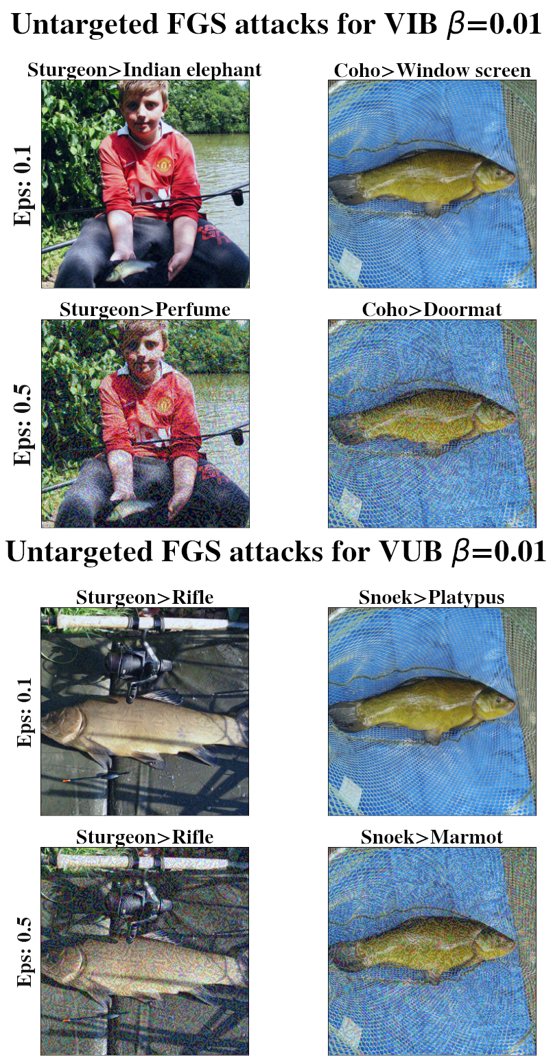
Figure 5: Successful untargeted FGS attack examples. Images are perturbations of previously successfully classified instances from the ImageNet validation set. Perturbation magnitude is determined by the parameter $\epsilon$ shown on the left, the higher the more perturbed. Original and wrongly assigned labels are listed at the top of each image. Notice the deterioration of image quality as $\epsilon$ increases.

Image classification evaluation results are shown in Table 1, examples of successful attacks are shown in Figures 4, 5. The empirical results presented in Table 1 confirm that while VIB and VUB reduce performance on the validation set, they substantially improve robustness to adversarial attacks. Moreover, these results demonstrate that VUB significantly outperforms VIB in terms of validation set accuracy while providing competitive robustness to attacks. A comparison of the best VIB and VUB models further substantiates these findings, with statistical significance confirmed by a p-value of less than 0.05 in a Wilcoxon rank sum test.

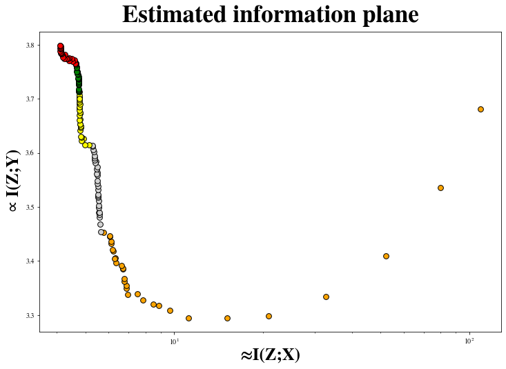
Figure 3: Estimated information plane metrics per epoch for VUB trained on the IMDB dataset with $\beta=0.001$. $I(Z;X)$ is approximated by $H(R)-H(Z|X)$ and $\frac{1}{CE(Y;\hat{Y})}$ is used as an analog for $I(Z;Y)$. The epochs have been grouped and color-coded in intervals of 30 epochs in the order: Orange (0-30), gray (30-60), yellow (60-90), green (90-120) and red (120-150). We notice recurring patterns of distortion reduction followed by rate increase, resembling the ERM and representation compression stages described by Shwartz-Ziv & Tishby (2017).

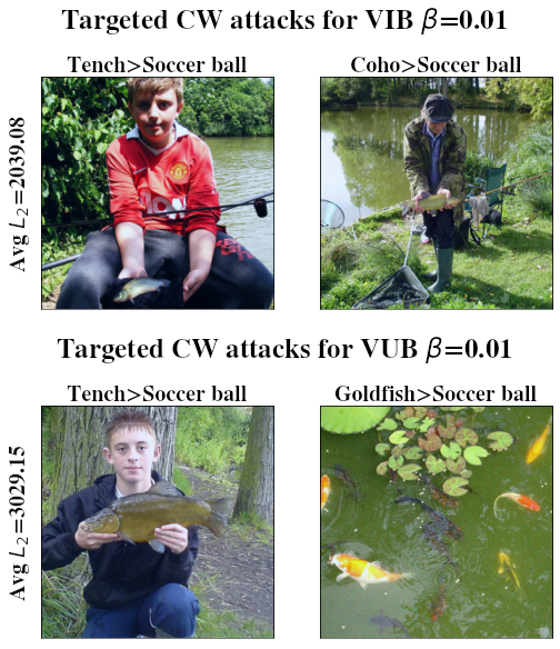
Figure 4: Successful targeted CW attack examples. Images are perturbations of previously successfully classified instances from the ImageNet validation set. The target label is ’Soccer ball’. Average $L_{2}$ distance required for a successful attack is shown on the left. The higher the required $L_{2}$ distance the greater the visible change required to fool the model. Original and wrongly assigned labels are listed at the top of each image. Mind the difference in noticeable change as compared to the FGS perturbations presented in Figure 5, and between VIB and VUB perturbations.

4.2 Text classification

A fine tuned BERT uncased Devlin et al. (2019) base model was used and achieved a 93.0% accuracy on the IMDB sentiment analysis test set. Each model was trained for 150 epochs. The entire test set was used to measure accuracy, while only the first 200 entries in the test set were used for adversarial attacks as they are computationally expensive.

4.2.1 Evaluation and analysis

Text classification evaluation results are shown in Table 2, examples of successful attacks are shown in Figure 3. In this modality VUB significantly outperforms VIB in both test set accuracy and robustness to both attacks. Moreover, VUB also outperomed the original model in terms of test set accuracy. A comparison of the best VIB and VUB models further substantiates these findings, with statistical significance confirmed by a p-value of less than 0.05 in a Wilcoxon rank sum test.

In addition to the above evaluation metrics, we also measured approximated rate and distortion throughout training and plotted them on the information curve as shown in Figure 3. We notice recurring patterns of distortion reduction followed by rate increase, resembling the ERM and representation compression stages described by Shwartz-Ziv & Tishby (2017).

$\beta$	Test$\uparrow$	DWB$\downarrow$	PWWS$\downarrow$
Vanilla model
-	93.0%	54.3%	100%
VIB models
$10^{-3}$	91.0% $\pm 1.0\%$	35.1% $\pm 4.4\%$	41.6% $\pm 6.6\%$
$10^{-2}$	90.8% $\pm 0.5\%$	41.0% $\pm 4.8\%$	62.9% $\pm 14.3\%$
$10^{-1}$	89.4% $\pm.9\%$	90.0% $\pm 8.0\%$	99.1% $\pm 0.9\%$
VUB models
$10^{-3}$	93.2% $\pm.5\%$	27.5% $\pm 2.0\%$	28.4% $\pm 1.3\%$
$10^{-2}$	92.6% $\pm.8\%$	30.8% $\pm 2.0\%$	50.0% $\pm 4.8\%$
$10^{-1}$	89.2% $\pm 2.0\%$	99.2% $\pm 0.5\%$	100% $\pm 0\%$

Table 2: Evaluation for vanilla, VIB and VUB models, average over 5 runs with standard deviation over the IMDB dataset. First column is performance on the test set (higher is better $\uparrow$), second is % of successful Deep Word Bug attacks (lower is better $\downarrow$) and the third column is % of successful PWWS attacks (lower is better $\downarrow$).

Text perturbed with DWB
gnreat historical movie, will not allow a viewer to leave once you begin to watch. View is presented differently than displayed by most school books on this sSubject […]
Text perturbed with PWWS
the acting , costumes , music , cinematography and sound are all astoundingdumbfounding given the production ’s austere locales .

Table 3: Examples of successful DWB and PWWS perturbations on a vanilla Bert model fine tuned over the IMDB dataset. The original input strings were perturbed such that inserted tokens are marked in underscored boldface and removed tokens in strikethrough. Both examples were classified correctly as ’Positive sentiment’ before the attack and ’Negative sentiment’ afterwards.

5 Discussion

While providing a complete framework for optimal data modeling, the IB, and it’s variational approximations, rely on three assumptions: (1) It suffices to optimize the mutual information metric to optimize a model’s performance; (2) Forgetting more information about the input while keeping the same information about the output induces better generalization; (3) Mutual information between the input, output and latent representation can be either computed or approximated to a desired level of accuracy. Our study strengthens the argument for using the Information Bottleneck combined with variational approximations to obtain robust models that can withstand adversarial attacks. By deriving a tighter bound on the IB functional, we demonstrate it’s utility as the Variational Upper Bound (VUB) objective for neural networks. We demonstrate that VUB outperforms the Variational Information Bottleneck (VIB) in terms of test accuracy while providing similar or superior robustness to adversarial attacks in challenging classification tasks of different modalities, suggesting an improvement in data modeling quality.

Comparing VIB and VUB we observe that both methods promote a disentangled latent space by using a stochastic factorized prior, as suggested by Chen et al. (2018). In addition, both methods utilize KL regularization, enforcing clustering around a $0$ mean which might increase latent smoothness. These traits can make it difficult for minor perturbations to significantly alter latent semantics, making the models more robust to attacks. In the case of VUB, the enhanced results induced by classifier regularization not only reinforce previous studies on the ELBO function, which suggest that overly powerful decoders diminish the quality of learned representations Alemi et al. (2018), but also align with the confidence penalty proposed by Pereyra et al. (2017).

In addition, we observed that in many cases VIB achieves lower validation set cross entropy while VUB achieves significantly higher test set accuracy. We attribute this gap to the VUB models becoming more calibrated, and we suggest that practitioners also monitor validation set accuracy and rate-distortion ratio during training. These metrics may be more informative indicators of model performance than validation set cross entropy alone, as validation cross entropy could increase as models become more calibrated.

We made another interesting observation during our study regarding information plane behavior throughout the training process. While previous research has documented the occurrence of error minimization and representation compression phases, our work revealed that these phases can occur in cycles throughout training. This finding is particularly noteworthy because previous studies observed this phenomenon in simple toy problems, whereas our research demonstrated it in complex tasks of high dimensionality with unknown distributions. This suggests that this information plane behavior is not limited to simplified scenarios but is a characteristic of the learning process in more challenging tasks as well.

In conclusion, while the IB and its variational approximations do not provide a complete theoretical framework for DNN data modeling and regularization, they offer a strong, measurable and theoretically grounded approach. VUB is presented as a tractable and tighter upper bound of the IB functional that can be easily adapted to any classifier DNN, including transformer based text classifiers, to significantly increase robustness to various adversarial attacks while inflicting minimal decrease in test set performance, and in some cases even increasing it.

This study opens many opportunities for further research. Besides further improvements to the upper bound, it is intriguing to use VUB in self-supervised learning and in generative tasks. Other possible directions, including measuring model calibration as proposed by Achille & Soatto (2018) are left for future work.

Impact

This paper presents work whose goal is to advance the field of Machine Learning. There are many potential societal consequences of our work, none which we feel must be specifically highlighted here.

References

- Achille & Soatto (2018) Achille, A. and Soatto, S. Information dropout: Learning optimal representations through noisy computation. IEEE Trans. Pattern Anal. Mach. Intell., 40(12):2897–2905, 2018. URL http://dblp.uni-trier.de/db/journals/pami/pami40.html#AchilleS18.
- Alemi et al. (2017) Alemi, A. A., Fischer, I., Dillon, J. V., and Murphy, K. Deep variational information bottleneck. In Proceedings of the International Conference on Learning Representations (ICLR), Google Research, 2017.
- Alemi et al. (2018) Alemi, A. A., Poole, B., Fischer, I., Dillon, J. V., Saurous, R. A., and Murphy, K. Fixing a broken elbo. In Proceedings of Machine Learning Research, volume 80, pp. 159–168, PMLR, 2018. URL http://dblp.uni-trier.de/db/conf/icml/icml2018.html#AlemiPFDS018.
- Amjad & Geiger (2020) Amjad, R. A. and Geiger, B. C. Learning representations for neural network-based classification using the information bottleneck principle. IEEE Trans. Pattern Anal. Mach. Intell., 42(9):2225–2239, 2020. URL http://dblp.uni-trier.de/db/journals/pami/pami42.html#AmjadG20.
- Blahut (1972) Blahut, R. E. Computation of channel capacity and rate distortion function. IEEE Transactions on Information Theory, IT-18:460–473, 1972. doi: https://ieeexplore.ieee.org/document/1054855. URL https://ieeexplore.ieee.org/document/1054855.
- Carlini & Wagner (2017) Carlini, N. and Wagner, D. A. Towards evaluating the robustness of neural networks. In IEEE Symposium on Security and Privacy, pp. 39–57. IEEE Computer Society, 2017. URL http://dblp.uni-trier.de/db/conf/sp/sp2017.html#Carlini017.
- Chechik et al. (2003) Chechik, G. et al. Gaussian information bottleneck. In Advances in Neural Information Processing Systems, 2003. URL https://proceedings.neurips.cc/paper/2003/hash/7e05d6f828574fbc975a896b25bb011e-Abstract.html.
- Chen et al. (2018) Chen, T. Q., Li, X., Grosse, R. B., and Duvenaud, D. Isolating sources of disentanglement in variational autoencoders. In Proceedings of the 32nd International Conference on Neural Information Processing Systems, pp. 2615–2625, 2018. URL http://dblp.uni-trier.de/db/conf/nips/nips2018.html#ChenLGD18.
- Deng et al. (2009) Deng, J., Dong, W., Socher, R., Li, L.-J., Li, K., and Fei-Fei, L. Imagenet: A large-scale hierarchical image database. In 2009 IEEE conference on computer vision and pattern recognition, pp. 248–255. Ieee, 2009.
- Devlin et al. (2019) Devlin, J., Chang, M.-W., Lee, K., and Toutanova, K. Bert: Pre-training of deep bidirectional transformers for language understanding. In Proceedings of the 2019 Conference of the North American Chapter of the Association for Computational Linguistics: Human Language Technologies, Volume 1 (Long and Short Papers), pp. 4171–4186, Minneapolis, Minnesota, 2019. URL https://www.aclweb.org/anthology/N19-1423.
- Fischer (2020) Fischer, I. The conditional entropy bottleneck. Entropy, 22(9):999, 2020. URL http://dblp.uni-trier.de/db/journals/entropy/entropy22.html#Fischer20.
- Gao et al. (2018) Gao, J., Lanchantin, J., Soffa, M. L., and Qi, Y. Black-box generation of adversarial text sequences to evade deep learning classifiers. In 2018 IEEE Security and Privacy Workshops (SPW), pp. 50–56. IEEE, 2018.
- Goodfellow et al. (2015) Goodfellow, I. J., Shlens, J., and Szegedy, C. Explaining and harnessing adversarial examples. In ICLR (Poster), 2015. URL http://dblp.uni-trier.de/db/conf/iclr/iclr2015.html#GoodfellowSS14.
- Guo et al. (2017) Guo, C., Pleiss, G., Sun, Y., and Weinberger, K. Q. On calibration of modern neural networks. In International conference on machine learning, pp. 1321–1330. PMLR, 2017.
- Higgins et al. (2017) Higgins, I., Matthey, L., Pal, A., Burgess, C., Glorot, X., Botvinick, M., Mohamed, S., and Lerchner, A. beta-vae: Learning basic visual concepts with a constrained variational framework. In ICLR (Poster), 2017.
- Kaiwen (2018) Kaiwen. pytorch-cw2, 2018. URL https://github.com/kkew3/pytorch-cw2. GitHub repository.
- Kingma & Welling (2014) Kingma, D. P. and Welling, M. Auto-encoding variational bayes. In 2nd International Conference on Learning Representations, ICLR 2014, Banff, AB, Canada, April 14-16, 2014, Conference Track Proceedings, 2014.
- Kingma & Welling (2019) Kingma, D. P. and Welling, M. An introduction to variational autoencoders. Foundations and Trends in Machine Learning, 12(4):307–392, 2019. URL http://dblp.uni-trier.de/db/journals/ftml/ftml12.html#KingmaW19.
- Maas et al. (2011) Maas, A., Daly, R. E., Pham, P. T., Huang, D., Ng, A. Y., and Potts, C. Learning word vectors for sentiment analysis. In Proceedings of the 49th annual meeting of the association for computational linguistics: Human language technologies, pp. 142–150, 2011.
- Morris et al. (2020) Morris, J., Lifland, E., Yoo, J. Y., Grigsby, J., Jin, D., and Qi, Y. Textattack: A framework for adversarial attacks, data augmentation, and adversarial training in nlp. In Proceedings of the 2020 Conference on Empirical Methods in Natural Language Processing: System Demonstrations, pp. 119–126, 2020.
- Painsky & Tishby (2017) Painsky, A. and Tishby, N. Gaussian lower bound for the information bottleneck limit. J. Mach. Learn. Res., 18:213:1–213:29, 2017. URL http://dblp.uni-trier.de/db/journals/jmlr/jmlr18.html#PainskyT17.
- Pereyra et al. (2017) Pereyra, G., Tucker, G., Chorowski, J., Kaiser, L., and Hinton, G. E. Regularizing neural networks by penalizing confident output distributions. In Proceedings of the International Conference on Learning Representations, OpenReview.net, 2017. URL http://dblp.uni-trier.de/db/conf/iclr/iclr2017w.html#PereyraTCKH17.
- Ren et al. (2019) Ren, S., Deng, Y., He, K., and Che, W. Generating natural language adversarial examples through probability weighted word saliency. In Proceedings of the 57th annual meeting of the association for computational linguistics, pp. 1085–1097, 2019.
- Shwartz-Ziv & Tishby (2017) Shwartz-Ziv, R. and Tishby, N. Opening the black box of deep neural networks via information, 2017. URL http://arxiv.org/abs/1703.00810. 19 pages, 8 figures.
- Slonim (2002) Slonim, N. The information bottleneck: Theory and applications. PhD thesis, Hebrew University of Jerusalem Jerusalem, Israel, 2002.
- Szegedy et al. (2016) Szegedy, C., Vanhoucke, V., Ioffe, S., Shlens, J., and Wojna, Z. Rethinking the inception architecture for computer vision. In Proceedings of the IEEE conference on computer vision and pattern recognition, pp. 2818–2826, 2016.
- Tishby & Zaslavsky (2015) Tishby, N. and Zaslavsky, N. Deep learning and the information bottleneck principle, 2015.
- Tishby et al. (1999) Tishby, N., Pereira, F. C., and Bialek, W. The information bottleneck method. In The 37th annual Allerton Conference on Communication, Control, and Computing., Hebrew University, Jerusalem 91904, Israel, 1999.
- Wieczorek & Roth (2019) Wieczorek, A. and Roth, V. On the difference between the information bottleneck and the deep information bottleneck. CoRR, abs/1912.13480, 2019. URL http://dblp.uni-trier.de/db/journals/corr/corr1912.html#abs-1912-13480.
- Ying (2019) Ying, X. An overview of overfitting and its solutions. Journal of Physics: Conference Series, 1168(2):022022, feb 2019. doi: 10.1088/1742-6596/1168/2/022022. URL https://dx.doi.org/10.1088/1742-6596/1168/2/022022.