Logistic Multidimensional Data Analysis for Ordinal Response Variables using a Cumulative Link function

Abstract

We present a multidimensional data analysis framework for the analysis of ordinal response variables. Underlying the ordinal variables, we assume a continuous latent variable, leading to cumulative logit models. The framework includes unsupervised methods, when no predictor variables are available, and supervised methods, when predictor variables are available. We distinguish between dominance variables and proximity variables, where dominance variables are analyzed using inner product models, whereas the proximity variables are analyzed using distance models. An expectation-majorization-minimization algorithm is derived for estimation of the parameters of the models. We illustrate our methodology with data from the International Social Survey Programme.

Keywords PCA  $\cdot$ MDU  $\cdot$ MM algorithm  $\cdot$ EM algorithm  $\cdot$ Maximum Likelihood  $\cdot$ Biplots

1 Introduction

In many fields of study, ordered categorical variables, also called ordinal variables, are collected. In medicine, for example, patients can be classified as, say, severely, moderately, or mildly ill (Anderson and Philips,, 1981). In the social and behavioural sciences, commonly Likert scales are used that have response categories such as "strongly disagree" (SD), "disagree" (D), "neutral" (N), "agree" (A), and "strongly agree" (SA). There is an ordering between these categories, but differences between these categories are unknown. It is standard practice to give numerical codes to the categories, such as 1, 2, 3, 4, 5, and subsequently perform a standard numerical analysis. In the context of regression modelling, Liddell and Kruschke, (2018) argue that the analysis of ordinal response variables through linear models can lead to distorted effect sizes, inflated Type-I errors, and inversions of differences between groups.

Underlying many ordinal variables, a continuous variable can be assumed. This is a latent variable, as we only observe the ordinal scores not the numerical ones. In Figure 1, we show the density of such a latent numerical variable. Instead of the numerical values, we observe categories such as SD, D, N, A, and SA. The continuous underlying variable is partitioned through a set of cut-points or thresholds into a set of categories. In Figure 1, the thresholds are shown as vertical dashed lines. All responses falling between two thresholds invoke the same response category. More formally, let $z$ be the continuous latent variable. Define a set of thresholds $-\infty=m_{0}<m_{1}<\ldots<m_{C}=\infty$ such that an observed ordinal response $y$ satisfies

$$y=c\ \ \mathrm{if}\ m_{c-1}\leq z<m_{c}$$

for $c=1,\ldots,C$.

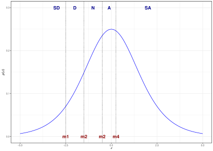
Figure 1: Probability density function for a continuous latent variable $z$ with thresholds (indicated by the vertical lines) giving rise to an observed ordered categorical variable with categories, strongly disagree (SD), disagree (D), neutral (N), agree (A), and strongly agree (SA).

In regression modeling of an ordinal response variable, the following model for the latent variable is assumed

$$z=\bm{x}^{\prime}\bm{\beta}+\epsilon,$$

where $\epsilon$ is an independent and identically distributed error term with cumulative density function $F$. This regression model for the latent response variable implies

$$P(y=c)=P(m_{c-1}<z\leq m_{c})=F\left(m_{c}-\bm{x}^{\prime}\bm{\beta}\right)-F\left(m_{c-1}-\bm{x}^{\prime}\bm{\beta}\right).$$

It follows that

$$F^{-1}\left(P(y\leq c|\bm{x})\right)=m_{c}-\bm{x}^{\prime}\bm{\beta},$$

where $\bm{x}^{\prime}\bm{\beta}$ is the structural part of the model.

In regression modelling, the de facto default choice for the analysis of categorical response variables are logistic models (Agresti,, 2002). For binary response variables, standard binary logistic regression models have been developed and these have been extended for ordinal variables and nominal variables (see Agresti,, 2002, chapter 7). In logistic regression models for ordinal variables, we use the cumulative density function of the logistic distribution, such that $F$ equals

$$F(\eta)=\frac{1}{1+\exp(-\eta)}$$

and the corresponding regression model is known as the proportional odds model, or, more generally, the cumulative logistic regression model (McCullagh,, 1980; Anderson and Philips,, 1981; Agresti,, 2002).

In many investigations, multiple response variables are collected. Researchers often analyze the response variables separately, but because the response variables are correlated this might not be an optimal strategy. Multidimensional data analysis refers to a set of data analysis techniques representing the multivariate data in a low dimensional, often Euclidean, space. The $R$ response variables are analyzed together and the results are represented in an $S$-dimensional space, where $S<R$. In the low dimensional representation, the associations (i.e., correlations) between response variables are modelled.

For the analysis of data it is important to distinguish between two types of response processes (Coombs,, 1964; Polak,, 2011). In a unipolar or cumulative scale or map, responses are monotonically related to the position of the person on the map. The response variables are so-called dominance variables. Mathematical problems are a typical example of dominance items where subjects with a higher mathematical ability have a higher probability of solving the problem correctly. In a bipolar scale or map, the variable responses are characterized by the proximity between the variable and the respondent: The responses are single-peaked functions of the distance between the position of a variable and the position of a person. The variables are so-called proximity variables. For dominance variables the subjects are partitioned into homogeneous groups, that is, all subjects with a fixed response constitute a homogeneous group. For proximity items, reasons to answer totally disagree might differ between the respondents. Respondents who disagree therefore do not necessarily constitute a homogeneous group.

In classical multivariate analysis, principal component analysis (PCA, Pearson,, 1901; Hotelling,, 1936; Jolliffe,, 2002) is the standard tool for the analysis of dominance data whereas multidimensional unfolding (MDU, Heiser,, 1981; Busing,, 2010) is the standard tool for the analysis of single-peaked processes.

In principal component analysis, a data set is summarized by reducing the dimensionality using a set of principal components, that are, linear combinations of the original variables, that explain as much of the original variability as possible. The data are summarized by principal scores and variable loadings. The principal scores are scores of the individuals on the principal components, while the variable loadings give the relation between the principal components and the original response variables. PCA solutions can be graphically represented through so-called biplots (Gabriel,, 1971; Gower and Hand,, 1996; Gower et al.,, 2011), where the row objects (observations, participants, individuals) are represented as points in a Euclidean space and the columns (variables, items) as vectors or variable axes. Estimated values of the responses can be obtained from the biplot by orthogonal projection of the row object points onto the variable axes.

Another multidimensional data analysis approach is multidimensional unfolding. Where PCA uses an inner-product representation of the data, MDU uses a distance representation. MDU is a generalization of multidimensional scaling to two-way two-mode data matrices (Carroll and Arabie,, 1980). In MDU, the data are approximated by the distance between so-called ideal points for the row objects (i.e., participants) and points for the response variables, that is, the distances between the two sets of points. MDU solutions can also be graphically represented by biplots, where both the row-objects and the variables are represented by points in a Euclidean space. Estimated values can be obtained by inspecting the distances between the two sets of points.

When besides the response variables also predictor variables are available on the row objects, we can constrain the PCA or MDU to incorporate this information. The principal scores or the ideal points are restricted to be (linear) functions of the predictor variables. When we constrain PCA in such a manner, the resulting model is known as reduced rank regression (RRR; Izenman,, 1975; Tso,, 1981) or redundancy analysis (Van den Wollenberg,, 1977). Reduced rank regression models can also be represented graphically, by so-called triplots (Ter Braak and Looman,, 1994). When we constrain MDU in such manner, we obtain a model known as restricted multidimensional unfolding (RMDU; Busing et al.,, 2010). These restricted multidimensional unfolding models can also be graphically represented by triplots.

PCA requires numerical data and estimation is usually done by minimizing a least squares function. Several extensions have been proposed to deal with other types of data. The first class of extensions have in common that the least squares criterion is maintained. For PCA of ordinal variables, Labovitz, (1970) proposed to use rank numbers instead of the numerical values. Korhonen and Siljamäki, (1998) proposed an ordinal PCA that maximizes the rank correlation between the original variables and the principal components. As PCA can also be conceived as an eigenvalue decomposition of the correlation matrix, Kolenikov and Angeles, (2004) argue to use an eigenvalue decomposition of the polychoric correlation matrix. Nonlinear Principal Component analysis has been proposed for the analysis of ordinal variables where an optimal transformation of the original variables is sought that minimizes the least squares loss function (Gifi,, 1990; Linting et al.,, 2007; Mori et al.,, 2016; Hoshiyar et al.,, 2021). The second class of extensions use other loss functions. For binary data, several authors (Schein et al.,, 2003; De Leeuw,, 2006; Landgraf and Lee,, 2020) proposed PCA using the binomial negative log-likelihood as loss function. Collins et al., (2001) proposed a generalization of PCA to the exponential family to deal with, for example, binary data or integer-valued data such as count data. As far as we know, there are no exponential family generalizations of PCA for ordinal response variables.

For constrained PCA, that is reduced rank regression or redundancy analysis, generalizations have been proposed for binary data (De Rooij,, 2023) and the exponential family (Yee and Hastie,, 2003). As far as we know, there are no exponential family generalizations of these reduced rank models for ordinal response variables.

MDU usually requires two-way two-mode data with non-negative values that can be interpreted as proximities. Metric MDU requires numerical proximity data. Non-metric MDU can deal with, for example, rank order data, but has been plagued by degeneracy problems for ages (for an overview see Busing, (2010), chapter 1). MDU has been generalized for binary variables by several authors (Andrich,, 1988; Takane,, 1998; DeSarbo and Hoffman,, 1986), using squared distances. Andrich, (1988) proposed a unidimensional model that does not allow for predictor variables. Takane, (1998) and DeSarbo and Hoffman, (1986) describe generalizations to multiple dimensions and explanatory versions. De Rooij et al., (2022) defined a model on the basis of (unsquared) distances for binary data, both with and without predictor variables. As far as we know, there are no exponential family generalizations of MDU for ordinal response variables.

In this manuscript, we will propose a family of geometric, multidimensional, models for multivariate ordinal data. We distinguish between dominance and proximity response variables. We also distinguish models with and without predictor variables. One unified algorithm for the estimation of model parameters will be presented (Section 3), where in the lower level iterations updates differ between the four approaches. We will also briefly discuss model selection issues. In Section 4, we show applications to data from the International Social Survey Programme (ISSP Research Group,, 2022). We end this paper with some conclusions.

2 Cumulative Logistic Multidimensional Models

We consider a set of ordinal variables $y_{ir}$ ($i=1,\ldots,N$, $r=1,\ldots,R$) where variable $r$ has $C_{r}$ categories, coded as $c=1,\ldots,C_{r}$. Underlying each ordered categorical response variable $y_{r}$ we assume a continuous latent variable $z_{r}$. We model these latent variables as

$$z_{ir}=\theta_{ir}+\epsilon_{ir},$$

where $\theta_{ir}$, the structural part of the model, is geometrically defined in $S$ dimensions. When using PCA we define

$$\theta_{ir}=\langle\bm{u}_{i},\bm{v}_{r}\rangle=\sum_{s=1}^{S}u_{is}v_{rs},$$

with $\bm{u}_{i}$ the principal scores and $\bm{v}_{r}$ the loadings, whereas

$$\theta_{ir}=-d(\bm{u}_{i},\bm{v}_{r})=-\sqrt{\sum_{s=1}^{S}(u_{is}^{2}+v_{rs}^{2}-2u_{is}v_{rs})},$$

with $\bm{u}_{i}$ the ideal points for participant $i$ and $\bm{v}_{r}$ the location for variable $r$ when MDU is used. We denote the two models by cumulative logistic PCA (CLPCA) and cumulative logistic MDU (CLMDU).

When predictor variables are available for the participants, the coordinates of the principal scores or ideal points can be restricted to be a linear, additive function of these predictor variables, that is $\bm{u}_{i}=\bm{B}^{\prime}\bm{x}_{i}$ with $\bm{B}$ a $P\times S$ matrix. Within the PCA context, we obtain the reduced rank regression model. For MDU, we obtain a restricted multidimensional unfolding.

We assume the $\epsilon_{ir}$ to be independent and identically distributed error terms following a cumulative logistic distribution. The probability density function of the logistic distribution equals

$$f(\eta)=\frac{\exp(-\eta)}{[1+\exp(-\eta)]^{2}}\ \mathrm{for}\ \eta\in\ (-\infty,\infty),$$

such that its logarithm is

$$\log f(\eta)=-\eta-2\log[1+\exp(-\eta)].$$

The cumulative density function of this distribution equals

$$F(\eta)=\frac{1}{1+\exp(-\eta)}\ \mathrm{for}\ \eta\in\ (-\infty,\infty).$$

It follows that

$$F^{-1}\left(P(y_{ir}\leq c)\right)=\log\left(\frac{P(y_{ir}\leq c)}{P(y_{ir}>c)}\right)=m_{r_{c}}-\theta_{ir},$$

where, similar to the proportional odds regression model, the thresholds are category specific but the structural part of the model is variable specific.

2.1 Properties of Cumulative Logistic Models

Let us consider two subjects with locations $\bm{u}_{1}$ and $\bm{u}_{2}$. The cumulative log-odds ratio for response variable $r$ is

$$\tau=\log\left(\frac{P(y_{1r}\leq c)}{P(y_{1r}>c)}\right)-\log\left(\frac{P(y_{2r}\leq c)}{P(y_{2r}>c)}\right).$$

With a PCA parameterisation, $\tau$ can be written as

$$\tau=m_{r_{c}}-\langle\bm{u}_{1},\bm{v}_{r}\rangle-(m_{r_{c}}-\langle\bm{u}_{2},\bm{v}_{r}\rangle)=\left\langle(\bm{u}_{2}-\bm{u}_{1}),\bm{v}_{r}\right\rangle,$$

which does not depend on $c$. This is the proportional odds assumption. Furthermore, if we define $\bm{u}_{2}$ as $\bm{u}_{2}=\bm{u}_{1}+\delta(\bm{u})$, such that $\delta(\bm{u})$ is a shift from one position to another, then we may write

$$\tau=\left\langle\delta(\bm{u}),\bm{v}_{r}\right\rangle,$$

which shows that it does not matter where in the Euclidean space this shift happens, the cumulative log-odds ratio remains constant for constant $\delta(\bm{u})$.

When $\bm{u}_{i}=\bm{B}^{\prime}\bm{x}_{i}$, we might be interested in the change of cumulative log-odds when one of the predictor variables increases by one unit. Say, the $p$-th predictor variable increases by a unit, such that, $\delta(\bm{u})=\bm{B}^{\prime}(\bm{x}_{2}-\bm{x}_{1})=\bm{b}_{p}$, then the cumulative log-odds increase by $\left\langle\bm{b}_{p},\bm{v}_{r}\right\rangle$.

Cumulative logistic reduced rank regression models can also be interpreted numerically, similar to the regression weights in proportional odds models. With reduced rank coefficient matrix $\bm{BV}^{\prime}$, each column of this matrix represents a change in cumulative log odds for a predictors unit increase.

For cumulative logistic MDU there is a nonlinear, distance relationship. Therefore, in contrast with the PCA parameterization, there is no such thing as a proportional odds assumption. The changes in cumulative log odds are not constant for changes in $\bm{u}$.

2.2 Model Selection

Assuming conditional independence between the response variables given the representation in low dimensional space, we will estimate the models by maximizing the likelihood (see Section 3, where we derive an algorithm). For selecting a model, that is, finding the optimal dimensionality and selecting a set of predictor variables, likelihood based statistics can be used. We propose to first select an optimal dimensionality, including all predictor variables if available, and thereafter select an optimal set of predictors. For dimensionality selection information criteria (AIC, BIC) can be used. After fixing the dimensionality, we can either use information criteria or likelihood ratio statistics for inference about the predictor variables. In the remainder of the paper, we will use information criteria.

For the AIC and BIC we need the number of parameters. In all our models, we have the threshold parameters, the number of which is $\sum_{r}(C_{r}-1)$. For reduced rank models, such as PCA and RRR, the number of parameters in the structural part is $(N+R-S)S$ and $(P+R-S)S$, respectively. Mukherjee et al., (2015) showed, in the context of linear reduced rank models, that these numbers are naive estimates, For linear reduced rank model better estimates are available, but this theory is not extended (yet) to other types of models, such as ordinal response variables. For MDU and RMDU, the number of parameters in the structural part is $(N+R)S-S(S+1)/2$ and $(P+R)S-S(S-1)/2$, respectively.

2.3 Biplots

2.3.1 CLPCA biplots

Biplots (Gower and Hand,, 1996; Gower et al.,, 2011) are useful displays for the results of a PCA, especially for two-dimensional solutions. We will now discuss the geometry of the two-dimensional biplot for Cumulative Logistic PCA. Like a usual PCA biplot, observations are shown as points, and variables are shown by axes. The coordinates of the points are given by the estimated $\bm{u}_{i}$. The variable axes are straight lines though the origin with direction $\frac{v_{r2}}{v_{r1}}$. In Figure 2a, we present a simplified biplot where the observations are shown by grey dots and there is a single variable axis (solid line). For this variable, $\bm{v}_{r}=[1,0.5]^{\prime}$ and suppose $m_{r_{c}}=(-2.0,-1.5,-0.5)$ for $c=1,2$ and $3$, respectively, i.e., thresholds for a four-point response scale. Estimated values for the response of an individual can be obtained by projecting the point representing this individual onto the variable axis. Subjects positioned in the lower left corner have lower expected values for the response, while subjects in the upper right corner have higher expected values, projecting higher onto the variable axis. To further increase interpretation and provide numerical values for the expected value, Gower and Hand, (1996) suggest to add labeled markers to the variable axis. For CLPCA there are several possibilities.

(a)

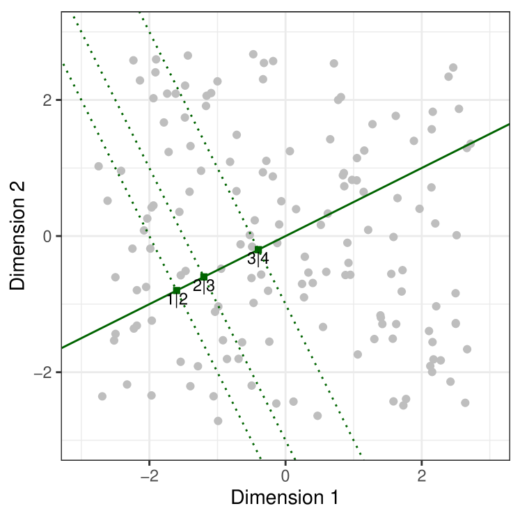
(b)

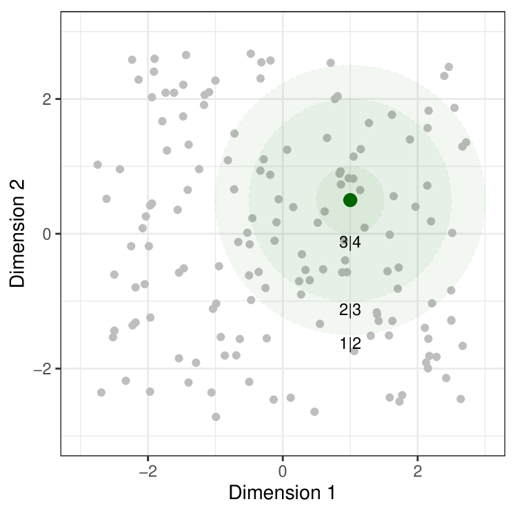
Figure 2: Biplot representations for CLPCA (left) and CLMDU (right) for a single response variable. Variable markers for cumulative probabilities are added. Grey points represent observations. On the left, the green solid line represents the variable axis with markers indicating the estimated thresholds. The dotted lines indicate decision regions for the categories of the response variable. On the right, the green point represents the response variable. The circles represent decision boundaries, where outside the circle the first category of the label is preferred and inside the circle the second category of the label.

Vicente-Villardón and Sánchez, (2014) suggest to add markers based on the largest estimated a posteriori probabilities. That is, for every point on the variable axis the probability for each response class is computed. At specific locations on the variable axis there are points where two categories, say $c$ and $c^{\prime}$, jointly have the highest probability. These points are marked as with $c|c^{\prime}$. They note that in some cases the probability of one or several categories are never higher than the probability of the other categories. When, for example, category 2 is such a ‘hidden’ category, the marker will be “1|3”.

In the context of the proportional odds model, Anderson and Philips, (1981) suggest to make predictions based on the underlying latent variable. Following this suggestion, we propose to add markers based on the underlying latent variable and the estimated thresholds. The predicted value of the latent variable is

$$\hat{z}_{ir}=\langle\hat{\bm{u}}_{i},\hat{\bm{v}}_{r}\rangle.$$

This inner product is constant ($\mu$, say) for all points on a line projecting at the same location of the variable axis. Therefore, the point of projection may be calibrated by labelling this point with the value $\mu$. This value also applies to the point of projection itself, which is $\lambda\bm{v}_{r}$. For the point $\lambda\bm{v}_{r}$ to be calibrated $\mu$, it must satisfy

$$\lambda\bm{v}_{r}^{\prime}\bm{v}_{r}=\mu,$$

so that $\lambda=\mu/\bm{v}_{r}^{\prime}\bm{v}_{r}$ and the coordinates of the point on the variable axis that is calibrated with a value of $\mu$ are $\mu\bm{v}_{r}/(\bm{v}_{r}^{\prime}\bm{v}_{r})$. As such, we would have the markers expressing values of the underlying latent continuous variable, but the interest lies in the observed ordinal response variable. The estimated response is $\hat{y}=c$ if $m_{r_{c-1}}\leq\hat{z}<m_{r_{c}}$. Therefore, markers can be based on the estimated thresholds (Anderson and Philips,, 1981). These markers indicate the transition points between adjacent categories. The coordinates of the marker point are given by $\hat{m}_{r_{c}}\bm{v}_{r}/(\bm{v}_{r}^{\prime}\bm{v}_{r})$ and these can be labeled by 1|2, 2|3, and so forth. The application of these markers is illustrated in Figure 2a. An advantage of these markers over the ones based on posterior probabilities is that each threshold is represented. The two-dimensional space can be partitioned into $C_{r}$ areas by drawing $C_{r}-1$ decision lines orthogonal on the variable axis and through the marker points, these are represented by the dotted lines in Figure 2a. In an usual biplot, several response variables are represented by variable axes jointly partitioning the two-dimensional space in open and closed regions that each represent a particular response profile.

2.3.2 CLMDU biplots

In MDU biplots, both the observations and the variables are shown by points in the two-dimensional space. The closer an observation to the variable point the higher the probability of a high response. To represent the ordinal nature of the response variable into the biplot, remember that we have

$$\log\left(\frac{P(y_{ir}\leq c)}{P(y_{ir}>c)}\right)=m_{r_{c}}+d(\bm{u}_{i},\bm{v}_{r}),$$

so that

$$\log\left(\frac{P(y_{ir}>c)}{P(y_{ir}\leq c)}\right)=-m_{r_{c}}-d(\bm{u}_{i},\bm{v}_{r})=a_{r_{c}}-d(\bm{u}_{i},\bm{v}_{r}).$$

It follows that we can add circles to the biplot with center $\bm{v}_{r}$ and radius $a_{r_{c}}$, such that for points inside this circle the probability for responding higher than $c$ is larger than 0.5 while outside the circle this probability is smaller or equal to 0.5. Every variable point is therefore accompanied with $C_{r}-1$ circles representing the different probabilities. We illustrate the threshold circles in Figure 2b, where again $\bm{v}_{r}=[1,0.5]^{\prime}$ and $m_{r_{c}}=(-2.0,-1.5,-0.5)$. From the $m_{r_{c}}$ we obtain $a_{r_{c}}=(2.0,1.5,0.5)$. In some cases the radius can be negative, indicating that nowhere in the two-dimensional space a cumulative probability is larger than a half, and the circle is not drawn. In an usual biplot, several response variables are represented, so we have several points with surrounding circles jointly partitioning the two-dimensional space. Again each region in this space represents a particular response profile.

2.4 Restricted Models

In case we have predictor variables available for the observations, the principal scores or ideal points ($\bm{u}_{i}$) are defined to be linear combinations of the predictor variables, that is $\bm{u}_{i}=\bm{B}^{\prime}\bm{x}_{i}$. Numerical predictor variables can be included in the two-dimensional biplot as straight lines through the origin and with direction $b_{p2}/b_{p1}$. The positions of the observations can be obtained from the predictor variable axes by the process of interpolation, as outlined by Gower and Hand, (1996).

Categorical predictor variables, are recoded into dummy variables, where one of the categories is chosen as a reference category. In the biplot representation, we use points instead of variable axes for such predictor variables. The position of the reference category is in the origin of the low dimensional space, whereas the other categories are positioned at their corresponding estimates in $\bm{B}$.

For interpretation, the relationship between a predictor variable and a response variable is of interest. In the CLPCA biplots, for numerical predictor variales such a relationship is given by the angle between a predictor variable axis and that of a response variable. A sharp angle indicates a strong relationship, while an obtuse angle indicates the absence of a relationship. Furthermore, for every point along the predictor variable axis, a projection onto the response variable axis can be made to obtain a predicted value. For categorical predictor, the point representing a category can be projected onto the response variable axis can be made to obtain a predicted value.

For CLMDU biplots, the interpretation of predictor-response relationships is more involved, because these are single-peaked where with increasing values of a predictor first the response goes up and afterwards down again. Furthermore, although the effect of predictor variables is additive for obtaining the position of an observation (i.e., the ideal point), this additivity does not translate to the relationship towards the response variable.

3 Maximum Likelihood Estimation

Assuming a multinomial distribution of the response variables, the observed data negative log-likelihood is

$$\mathcal{L}_{o}(\bm{\theta},\bm{m})=-\sum_{i}\sum_{r}\mathds{1}(y_{ir}=c)\log\pi_{irc},$$

where $\pi_{irc}=F(m_{r_{c}}-\theta_{ir})-F(m_{r_{c-1}}-\theta_{ir})$, and $\mathds{1}()$ is an indicator function of its argument, $\bm{\theta}$ collects all the structural parameters and $\bm{m}$ collects all the threshold parameters.

In this section, we will develop an Expectation Majorization Minimization (EMM) algorithm to minimize the negative loglikelihood. We start by formulating the complete data negative loglikelihood, take the conditional expectation of this function in the E-step, and find a majorization function that can easily be minimized. The majorization function turns out to be a least squares function, so that in the inner loop of the algorithm, well known updating steps from least squares theory can be used.

3.1 Estimation of Structural part

The complete data negative log-likelihood (CDNLL) is defined for the latent responses, that is

$$\mathcal{L}_{c}(\bm{\theta})=-\sum_{i}\sum_{r}\log f(z_{ir}-\theta_{ir}),$$

where $f(\cdot)$ is the probability density function of the logistic distribution (see Section 2). A second-order Taylor expansion of the complete data negative log-likelihood around current values $\tilde{\bm{\theta}}$ is

$$\mathcal{L}_{c}(\bm{\theta})=\mathcal{L}_{c}(\tilde{\bm{\theta}})+(\bm{\theta}-\tilde{\bm{\theta}})^{\prime}\frac{\partial\mathcal{L}_{c}(\tilde{\bm{\theta}})}{\partial\bm{\theta}}+\frac{1}{2}(\bm{\theta}-\tilde{\bm{\theta}})^{\prime}\frac{\partial^{2}\mathcal{L}_{c}(\tilde{\bm{\theta}})}{\partial\bm{\theta}\partial\bm{\theta}^{\prime}}(\bm{\theta}-\tilde{\bm{\theta}}).$$

In the E-step, the expectation of the complete data negative log-likelihood is obtained, that is

$$\mathbb{E}(\mathcal{L}_{c}(\bm{\theta}))=\mathbb{E}(\mathcal{L}_{c}(\tilde{\bm{\theta}}))+(\bm{\theta}-\tilde{\bm{\theta}})^{\prime}\mathbb{E}\left(\frac{\partial\mathcal{L}_{c}(\tilde{\bm{\theta}})}{\partial\bm{\theta}}\right)+\frac{1}{2}(\bm{\theta}-\tilde{\bm{\theta}})^{\prime}\mathbb{E}\left(\frac{\partial^{2}\mathcal{L}_{c}(\tilde{\bm{\theta}})}{\partial\bm{\theta}\partial\bm{\theta}^{\prime}}\right)(\bm{\theta}-\tilde{\bm{\theta}})$$

As the expectation of a sum is the sum of expectations, we can write

$$\mathbb{E}(\mathcal{L}_{c}(\bm{\theta}))=\sum_{i}\sum_{r}\mathbb{E}(\mathcal{L}_{c}(\theta_{ir})),$$

with

$$\mathbb{E}(\mathcal{L}_{c}(\theta_{ir}))=\mathbb{E}(\mathcal{L}_{c}(\tilde{\theta}_{ir}))+(\theta_{ir}-\tilde{\theta}_{ir})\mathbb{E}\left(\frac{\partial\mathcal{L}_{c}(\tilde{\theta}_{ir})}{\partial\theta_{ir}}\right)+\frac{1}{2}(\theta_{ir}-\tilde{\theta}_{ir})\mathbb{E}\left(\frac{\partial^{2}\mathcal{L}_{c}(\tilde{\theta}_{ir})}{\partial^{2}\theta_{ir}}\right)(\theta_{ir}-\tilde{\theta}_{ir}).$$

An upper bound for the (expectation of the) second derivative is given by $1/4$ such that

$$\mathbb{E}(\mathcal{L}_{c}(\theta_{ir}))\leq\mathbb{E}(\mathcal{L}_{c}(\tilde{\theta}_{ir}))+(\theta_{ir}-\tilde{\theta}_{ir})\mathbb{E}\left(\frac{\partial\mathcal{L}_{c}(\tilde{\theta}_{ir})}{\partial\theta_{ir}}\right)+\frac{1}{8}(\theta_{ir}-\tilde{\theta}_{ir})(\theta_{ir}-\tilde{\theta}_{ir})=\mathcal{M}(\theta_{ir}|\tilde{\theta}_{ir}).$$

Let us define $p_{ir}=\frac{1}{1+\exp(-z_{ir}+\theta_{ir})}$ such that $\log f(z_{ir}-\theta_{ir})=\log p_{ir}(1-p_{ir})$. The partial derivative is

$$\frac{\partial\mathcal{L}_{c}(\tilde{\theta}_{ir})}{\partial\theta_{ir}}=-\frac{\partial\log f(z_{ir}-\theta_{ir})}{\partial\theta_{ir}}=1-2p_{ir}.$$

We need the expectation of $p_{ir}$ to find the expectation of this partial derivative. Following Jiao, (2016), we derived the following closed form expressions (we use $p$, $y$ and $\theta$ instead of $p_{ir}$, $y_{ir}$ and $\theta_{ir}$ for readibility):

$$\mathbb{E}(p|y,\theta,m)=\left\{\begin{array}[]{ll}\left[\frac{\exp(2m_{y}-2\theta)}{2[\exp(m_{y}-\theta)+1]^{2}}\right]/F(m_{y}-\theta)&\mathrm{if}\ y=1\\[4.0pt] \left[\frac{2\exp(m_{(y-1)}-\theta)+1}{2[\exp(m_{(y-1)}-\theta)+1]^{2}}-\frac{2\exp(m_{y}-\theta)}{2[\exp(m_{y}-\theta)+1]^{2}}\right]/\left(F(m_{y}-\theta)-F(m_{(y-1)}-\theta)\right)&\mathrm{if}\ 2\leq y<C\\[4.0pt] \left[\frac{2\exp(m_{(y-1)}-\theta)+1}{2[\exp(m_{(y-1)}-\theta)+1]^{2}}\right]/\left(1-F(m_{(y-1)}-\theta)\right)&\mathrm{if}\ y=C\end{array}\right.$$

The expectation has to be evaluated at the current estimates of $\bm{\theta}$ and $\bm{m}$. Let us denote by $\xi_{ir}$ the expected value of the first derivative, that is

$$\xi_{ir}=1-2\mathbb{E}(p_{ir}|y_{ir},\theta_{ir},m_{r}),$$

so that the majorization function to be minimized is

$$\mathcal{M}(\bm{\theta}|\tilde{\bm{\theta}})=\sum_{i}\sum_{r}\mathcal{M}(\theta_{ir}|\tilde{\theta}_{ir})=\sum_{i}\sum_{r}\mathbb{E}(\mathcal{L}_{c}(\tilde{\theta}_{ir}))+(\theta_{ir}-\tilde{\theta}_{ir})\xi_{ir}+\frac{1}{8}(\theta_{ir}-\tilde{\theta}_{ir})(\theta_{ir}-\tilde{\theta}_{ir}).$$

Let us simplify this majorization function. Focusing on the individual elements, the first term is a constant ($c_{1}=\mathbb{E}(\mathcal{L}_{c}(\tilde{\theta}_{ir}))$) and therefore we focus on the other terms

$$\mathcal{M}(\theta_{ir}|\tilde{\theta}_{ir}) =c_{1}+\xi_{ir}(\theta_{ir}-\tilde{\theta}_{ir})+\frac{1}{8}(\theta_{ir}-\tilde{\theta}_{ir})(\theta_{ir}-\tilde{\theta}_{ir})$$

$$=c_{1}+\xi_{ir}\theta_{ir}-\xi_{ir}\tilde{\theta}_{ir}+\frac{1}{8}(\theta_{ir}^{2}+\tilde{\theta}_{ir}^{2}-2\theta_{ir}\tilde{\theta}_{ir})$$

$$=c_{1}+\frac{1}{8}\theta_{ir}^{2}+\xi_{ir}\theta_{ir}-2\frac{1}{8}\theta_{ir}\tilde{\theta}_{ir}-\xi_{ir}\tilde{\theta}_{ir}+\frac{1}{8}\tilde{\theta}_{ir}^{2}.$$

Let $\lambda_{ir}=\tilde{\theta}_{ir}-4\xi_{ir}$ to obtain

$$\mathcal{M}(\theta_{ir}|\tilde{\theta}_{ir}) =c_{1}+\frac{1}{8}\theta_{ir}^{2}-2\frac{1}{8}\theta_{ir}\lambda_{ir}+\frac{1}{8}\lambda_{ir}^{2}-\frac{1}{8}\lambda_{ir}^{2}-\xi_{ir}\tilde{\theta}_{ir}+\frac{1}{8}\tilde{\theta}_{ir}^{2}$$

$$=c_{1}+\frac{1}{8}(\theta_{ir}-\lambda_{ir})^{2}-\frac{1}{8}\lambda_{ir}^{2}-\xi_{ir}\tilde{\theta}_{ir}+\frac{1}{8}\tilde{\theta}_{ir}^{2}.$$

Define $c_{2}=c_{1}-\frac{1}{8}\lambda_{ir}^{2}-\xi_{ir}\tilde{\theta}_{ir}+\frac{1}{8}\tilde{\theta}_{ir}^{2}$, a constant with respect to $\theta_{ir}$, so that we can write

$$\mathbb{E}(\mathcal{L}_{ir}(\theta_{ir}))\leq\mathcal{M}(\theta_{ir}|\tilde{\theta}_{ir})=\frac{1}{8}(\theta_{ir}-\lambda_{ir})^{2}+c_{2}.$$

Now collecting all terms into a single function again, we obtain

$$\mathbb{E}(\mathcal{L}_{c}(\bm{\theta}))\leq\mathcal{M}(\bm{\theta}|\tilde{\bm{\theta}})=\frac{1}{8}\sum_{i}\sum_{r}(\theta_{ir}-\lambda_{ir})^{2}+c_{2}.$$

In the following four subsections, we work out this least squares loss function for the four different definitions of the structural part ($\theta_{ir}$).

3.1.1 PCA parametrisation of the Structural part

Remember that $\theta_{ir}=\langle\bm{u}_{i},\bm{v}_{r}\rangle$, so that the loss function in matrix algebra terms is

$$\bm{\Lambda}=\bm{U}\bm{V}^{\prime},$$

that is, we have to find a reduced rank approximation of the matrix $\bm{\Lambda}$ with elements $\lambda_{ir}$. Eckart and Young, (1936) showed that this can be done using a singular value decomposition

$$\bm{\Lambda}=\bm{P}\bm{\Phi}\bm{Q}^{\prime}$$

and defining the updates

$$\bm{U}^{+} = \sqrt{N}\bm{P}_{S}$$ (2)

$$\bm{V}^{+} = \frac{1}{\sqrt{N}}\bm{Q}_{S}\bm{\Phi}_{S},$$ (3)

where $\bm{P}_{S}$ and $\bm{Q}_{S}$ are the first $S$ singular vectors, and $\bm{\Phi}_{S}$ is the $S\times S$ diagonal matrix with the largest singular values.

3.1.2 RRR parametrisation of the Structural part

Compared to the PCA parametrisation, we impose the constraint that $\bm{u}_{i}=\bm{B}^{\prime}\bm{x}_{i}$. Therefore, in each iteration, we have to minimize

$$\|\bm{\Lambda}-\bm{XB}\bm{V}^{\prime}\|^{2}$$

over the parameters $\bm{B}$ and $\bm{V}$. Updates of $\bm{B}$ and $\bm{V}$ can be obtained from a generalized singular value decomposition of the matrix

$$(\bm{X}^{\prime}\bm{X})^{-1}\bm{X}^{\prime}\bm{\Lambda}$$

in the metrics $(\bm{X}^{\prime}\bm{X})$ and $\bm{I}$ (Takane,, 2013). Let

$$(\bm{X}^{\prime}\bm{X})^{-\frac{1}{2}}\bm{X}^{\prime}\bm{\Lambda}=\bm{P}\bm{\Phi}\bm{Q}^{\prime}$$

be the SVD. The updates are defined as

$$\bm{B}^{+} = \sqrt{N}(\bm{X}^{\prime}\bm{X})^{-\frac{1}{2}}\bm{P}_{S}$$ (4)

$$\bm{V}^{+} = \frac{1}{\sqrt{N}}\bm{Q}_{S}\bm{\Phi}_{S},$$ (5)

where $\bm{P}_{S}$ and $\bm{Q}_{S}$ are the first $S$ singular vectors, and $\bm{\Phi}_{S}$ is the $S\times S$ diagonal matrix with the largest singular values.

3.1.3 MDU parametrisation of the Structural part

The loss function in every iteration is

$$\frac{1}{8}\sum_{i}\sum_{r}(\theta_{ir}-\lambda_{ir})^{2}+c_{2}.$$

where $\theta_{ir}=-d(\bm{u}_{i},\bm{v}_{r})$ with $\bm{u}_{i}$ and $\bm{v}_{r}$ the parameters. This loss function can be rewritten as

$$\sum_{i}\sum_{r}w_{ir}(\delta_{ir}-d(\bm{u}_{i},\bm{v}_{r}))^{2},$$

where $\delta_{ir}=-\lambda_{ir}$ and $w_{ir}=1$, which is the usual raw STRESS function often used in multidimensional scaling and unfolding. De Leeuw, (1977) and De Leeuw and Heiser, (1977) proposed the SMACOF algorithm for minimization of this STRESS function for multidimensional scaling. The SMACOF algorithm is itself an MM algorithm. Convergence properties of this algorithm are described by De Leeuw, (1988). Heiser, (1981, 1987) showed that multidimensional unfolding can be considered a special case of multidimensional scaling. Subsequently, he developed the SMACOF algorithm to deal with rectangular proximity matrices. Advances in the algorithm are described in Busing, (2010). An elementary treatment of the algorithm for multidimensional scaling can be found in Chapter 8 of Borg and Groenen, (2005) and for multidimensional unfolding in Chapter 14. The critical difference with the usual loss function is that the dissimilarities $\delta_{ir}$ might be negative. Heiser, (1991) showed a way to deal with negative dissimilarities in multidimensional scaling. The line of thought of Heisers contribution is that two majorizing functions are defined: one for the case that the dissimilarity is positive and one for the case that the dissimilarity is negative. It turns out that the new algorithm is a simple adaptation of the standard SMACOF algorithm, where only some elements of two matrices ($\bm{A}$ and $\bm{W}$, see below) are defined differently, depending on the sign of the dissimilarity. De Rooij and Busing, (2022) and De Rooij et al., (2022) adapted Heiser’s algorithm for the multidimensional unfolding case. Here, we will follow that approach. We will only show the updating equations, for the derivation of these equations we refer to the above papers.

Define matrix $\bm{A}$ with elements $\{a_{ir}\}$ as follows

$$a_{ir}=\left\{\begin{array}[]{ll}w_{ir}\delta_{ir}/d(\bm{u}_{i},\bm{v}_{r})&\mathrm{if}\ \delta_{ir}\geq 0\ \mathrm{and}\ d(\bm{u}_{i},\bm{v}_{r})>0\\ 0&\mathrm{else}\end{array}\right..$$

Furthermore, redefine the weight matrix $\bm{W}$ with elements $\{w_{ir}\}$ as

$$w_{ir}=\left\{\begin{array}[]{ll}w_{ir}&\mathrm{if}\ \delta_{ir}\geq 0\\ \left[w_{ir}(d(\bm{u}_{i},\bm{v}_{r})+|\delta_{ir}|)\right]/d(\bm{u}_{i},\bm{v}_{r})&\mathrm{if}\ \delta_{ir}<0\ \mathrm{and}\ d(\bm{u}_{i},\bm{v}_{r})>0\\ \left[w_{ir}(\epsilon+\delta_{ir}^{2})\right]/\epsilon&\mathrm{if}\ \delta_{ir}<0\ \mathrm{and}\ d(\bm{u}_{i},\bm{v}_{r})=0\end{array}\right.,$$

where $\epsilon$ is a small constant. Note that the matrices $\bm{W}$ and $\bm{A}$ change from iteration to iteration.

Let us now define $\bm{R}=\mathrm{diag}(w_{i+})$, $\bm{C}=\mathrm{diag}(w_{+r})$, $\bm{P}=\mathrm{diag}(a_{i+})$, and $\bm{Q}=\mathrm{diag}(a_{+r})$, where the + in the subscript means taking the sum over the replaced index, that is, $w_{i+}=\sum_{r=1}^{R}w_{ir}$. With these matrices the update for $\bm{U}$ is

$$\bm{U}^{+}=\bm{R}^{-1}\left(\bm{P}\bm{U}-\bm{A}\bm{V}+\bm{W}\bm{V}\right)$$ (8)

and for $\bm{V}$ the update is

$$\bm{V}^{+}=\bm{C}^{-1}\left(\bm{Q}\bm{V}-\bm{A}^{\prime}\bm{U}^{+}+\bm{W}^{\prime}\bm{U}^{+}\right).$$ (9)

These updates are the same as in the standard least squares unfolding algorithm (see Busing,, 2010, pp. 176, 183-187), where only the definitions of $\bm{A}$ and $\bm{W}$ are changed.

3.1.4 RMDU parametrisation of the Structural part

In the supervised analysis, we have that $\bm{U}=\bm{XB}$ and we need to estimate $\bm{B}$ instead of $\bm{U}$. Given the other parameters, the update of $\bm{B}$ is given as

$$\bm{B}^{+}=\left(\bm{X}^{\prime}\bm{R}\bm{X}\right)^{-1}\left[\bm{X}^{\prime}\left(\bm{P}\bm{U}-\bm{A}\bm{V}\right)+\bm{X}^{\prime}\bm{W}\bm{V}\right]$$ (10)

and before updating $\bm{V}$ using Equation 9, we compute $\bm{U}^{+}=\bm{XB}^{+}$.

3.2 Estimation of thresholds

To update the threshold parameters for each response variable we cannot use the complete data negative log-likelihood. However, we can use the default maximum likelihood estimator as in the proportional odds regression model. For this estimator $\bm{y}_{r}$ is the response variable and we use $\bm{\theta}_{r}$ as an offset without further predictor variables, so this gives estimates of the intercepts or thresholds. This provides estimates for response variable $r$. We repeat the procedure for each response variable.

3.3 Remarks on Algorithms

The algorithms as outlined above monotonically converge to a local minimum of the negative log likelihood function. For the models based on the inner product (PCA and RRR) this local minimum is also the global minimum. For models based on the distance representation, however, local optima occur. To deal with these local optima, starting values near the global minimum might help, such as given by, for example, correspondence analysis. As such a start does not guarantee to find the global minimum, supplementary multiple random starts are advised.

4 Application

We will use data from the International Social Survey Programme 2020, the Module on Environment, to illustrate our methods (ISSP Research Group,, 2022). The data we will use has $N=16465$ observations (7917 Male and 8548 Female) from 13 different countries and concerns attitudes and behavior related to environmental issues.

The thirteen countries are Austria (AT, 1112), Taiwan (TW, 1574), Finland (FI, 942), Germany (DE, 1365), Hungary (HU. 856), Iceland (IS, 867), Japan (JP, 964), New Zealand (NZ, 807), Philippines (PH, 1346), Russia (RU, 959), Slovenia (SL, 960), Switzerland (CH, 3650), and Thailand (TH, 1063). Also available are two background variables that will be used as predictors, Education was measured by the number of years education received, and working status with three classes.

The survey includes four pro-environmental behavior variables, measured on ordinal scales:

• In the last twelve months how often, if at all, have you engaged in any leisure activities outside in nature, such as hiking, bird watching, swimming, skiing, other outdoor activities or just relaxing? Answers on a 5-point scale: daily (coded 5), several times a week (4), several times a month (3), several times a year (2), and never (1);

• In a typical week, on how many days do you eat beef, lamb, or products that contain them? Answers on a 8-point scale, 0 (coded 8), 1 (7), 2 (6), 3 (5), 4 (4), 5 (3), 6 (2), 7 (1), where numbers between brackets indicate our coding with higher numbers for more pro-environmental behaviour;

• How often do you make a special effort to sort glass or tins or plastic or newspapers and so on for recycling? Answers on a 4-point scale, always (4), often (3), sometimes (2), never (1);

• How often do you avoid buying certain products for environmental reasons? Answers on a 4-point scale: always (coded 4), often (3), sometimes (2), and never (1).

Environmental concern was measured by the following statement: Generally speaking, how concerned are you about environmental issues, where participants could respond on a 5-point scale ranging from "Not at all concerned" (1) till "Very concerned" (5).

Environmental efficacy was measured by the following seven statements that each had a 5-point answer scale ranging from Agree Strongly (coded as 5) to Disagree Strongly (coded as 1):

• It is just too difficult for someone like me to do much about the environment;

• I do what is right for the environment, even when it costs more money or takes more time;

• There are more important things to do in life than protect the environment;

• There is no point in doing what I can for the environment unless others do the same;

• Many of the claims about environmental threats are exaggerated;

• I find it hard to know whether the way I live is helpful or harmful to the environment;

• Environmental problems have a direct effect on my everyday life.

4.1 Cumulative Logistic Reduced Rank Regression

In this analysis, we take the four behavioural items as response variables. Predictors are environmental concern (treated as a numeric variable) and environmental efficacy which we obtained by taking the average over the seven items (after reverse coding of Item 2). Other predictors we used are country, gender, education, and work status. In psychological research, the relationship between attitudes and behaviour is often of interest. Therefore, our primary focus is on the relationship between environmental concern and efficacy and the four behavioural items, controlling for the other variables.

Model	S	Predictors	deviance	npar	AIC	BIC
1	1	All	169060.06	39	169138.06	169438.71
2	2	All	164644.90	59	164762.90	165217.74
3	3	All	162513.15	77	162667.15	163260.74
4	3	All - C	173682.04	41	173764.04	174080.11
5	3	All - G	162897.44	74	163045.44	163615.91
6	3	All - E	162644.64	74	162792.64	163363.11
7	3	All - W	162548.75	71	162690.75	163238.09
8	3	All - A	163119.68	74	163267.68	163838.15
9	3	All - EC	163164.41	74	163312.41	163882.87
10	3	All - EE	163487.87	74	163635.87	164206.34
11	3	All - W - C	173786.77	35	173856.77	174126.59
12	3	All - W - G	162938.51	68	163074.51	163598.72
13	3	All - W - E	162678.07	68	162814.07	163338.28
14	3	All - W - A	163378.23	68	163514.23	164038.45
15	3	All - W - EC	163201.58	68	163337.58	163861.79
16	3	All - W - EE	163487.87	74	163635.87	164206.34

Table 1: Model selection for ISSP data from cumulative logistic reduced rank regression. Abbreviations: C: Country, G: Gender, E: Education, W: Work, A: Age, EC: Environmental Concern, EE: Environmental Efficacy.

We start with a predictor matrix $\bm{X}$ of dimension 16696 by 19. First, we need to find an optimal dimensionality (rank). The model with $S=3$ has the lowest AIC and BIC, see Table 1. In the next step, we delete one by one the predictor variables from the model and see whether the AIC and BIC improve. Only for the variable work status the BIC decreases, but the AIC increases. After leaving out working status, we checked whether any other predictor can be left out, which is not the case. Model 7, with 71 parameters is the preferred model.

The estimated reduced rank coefficients (i.e., $\bm{BV}^{\prime}$) from Model 7 are displayed in Table 2. Note that Thailand (TH) serves as a reference country, so all regression coefficients for the countries should be compared to Thailand. For example, the cumulative log odds for Austria (AT) is 2.64 higher for leisure activities outside in nature (OUT), 0.69 lower for eating meet (MEAT), 1.93 higher for special effort to sort glass or tins or plastic or newspapers (RECYCLE), and 0.66 higher for avoiding to buy products for environmental reasons (AVOID). Checking our variables of interest, we see that when environmental concern (EC) and environmental efficacy (EE) increase the cumulative log odds for pro environmental behavior goes up, most strongly for environmental efficacy. For example, with every standard deviation increase in environmental efficacy the cumulative log odds for special effort to sort glass/tins/plastic/newspapers (RECYCLE) goes up by 0.46.

	OUT	MEAT	RECYCLE	AVOID
1|2	-1.28	-3.84	-2.50	-1.53
2|3	0.53	-3.26	-0.74	0.95
3|4	2.03	-2.48	0.83	3.38
4|5	3.91	-1.79
5|6		-0.96
6|7		-0.09
7|8		1.22
AT	2.64	-0.69	1.93	0.66
TW	0.45	1.19	1.51	1.02
FI	2.46	-1.02	1.60	0.44
DE	2.75	-0.38	2.18	0.82
HU	1.14	1.66	0.66	0.34
IS	2.28	-1.51	1.48	0.36
JP	-0.44	-0.82	1.38	0.95
NZ	2.20	-1.65	1.74	0.54
PH	-0.36	0.60	0.52	0.48
RU	0.83	-0.18	-1.24	-1.03
SL	3.19	-0.27	1.73	0.44
CH	2.66	-0.81	2.42	0.97
Female	0.03	0.50	0.22	0.18
Eduyrs	0.03	-0.02	0.19	0.12
age	0.10	0.14	0.40	0.26
EC	0.02	0.10	0.36	0.25
EE	0.19	0.20	0.46	0.28

Table 2: Estimated regression coefficients $\bm{BV}^{\prime}$ for the four pro-environmental behaviours.

4.2 Cumulative Logistic Restricted Multidimensional Unfolding

In this analysis, we like to see whether there are differences between countries concerning environmental efficacy. The seven ordinal items are treated as the responses ($R=7$) and the dummy variables for countries are used as predictors ($P=13-1=12$).

We fitted models in 1, 2, and 3 dimensions. The fit statistics are

	deviance	npar	AIC	BIC
1	316958.70	47.00	317052.70	317415.03
2	315116.83	65.00	315246.83	315747.92
3	314289.43	82.00	314453.43	315085.57

showing that the three-dimensional model fits best.

For illustrative purposes, the two-dimensional biplot is shown in Figure 3. We can discern three groups of countries: on the upper right there are the Asian countries (Taiwan, Japan, Philippines, and Thailand), on the bottom there are the East European countries Russia and Hungary, while on the left hand side there are the more Western countries (Austria, Finland, Germany, Iceland, New Zealand, Slovenia, and Switzerland).

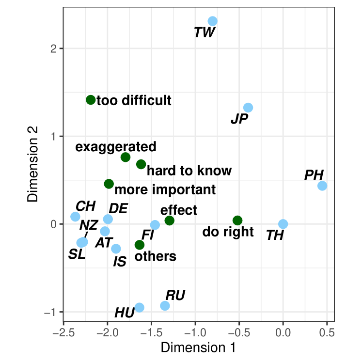
Figure 3: Estimated configuration for Environmental Efficacy data.

Considering the items, we see that Items 1, 3, 5, and 6 are quite close together, all showing hesitation of personal options (i.e., It is just too difficult for someone like me to do much about the environment; There are more important things to do in life than protect the environment; Many of the claims about environmental threats are exaggerated; I find it hard to know whether the way I live is helpful or harmful to the environment)

Items 4 and 7 are close together but a bit apart from the first cluster (There is no point in doing what I can for the environment unless others do the same; Environmental problems have a direct effect on my everyday life). Item 2 (I do what is right for the environment, even when it costs more money or takes more time) is a bit isolated on the right hand side.

To better visualize the differences between average opinions of people from the different countries, in Figure 4 we show the decision regions for two items (2 and 4). For item 2 (left hand side), the estimated radii corresponding to the thresholds 3|4 and 4|5 are negative, so these circles are not shown. The interpretation is that in none of the countries the average opinion is to agree or strongly agree with this assertion. Therefore, the 13 countries are partitioned into two groups, those who neither disagree nor agree (Finland, Thailand, and the Philippines) and those who disagree (Taiwan, Japan, Russia, Hungary, Austria, Germany, Iceland, New Zealand, Slovenia, and Switzerland). The people from these countries, however, disagree for different reasons as the positions for the countries are on different sides of the item. For Item 4, the estimated radius corresponding to the threshold 4|5 is negative, so this circle is not shown. It can be verified that on average the Taiwanese, Japanese, and Philippine people disagree with this statement, while people from Thailand neither agree nor disagree, and all others countries generally agree with the statement.

(a)

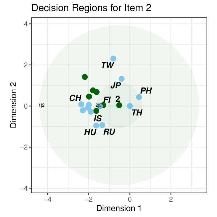
(b)

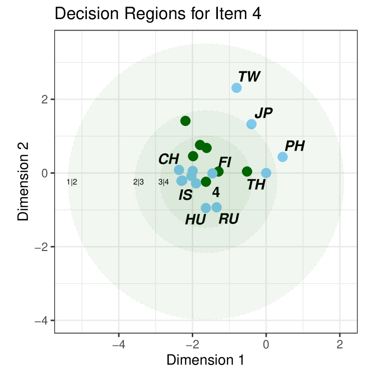
Figure 4: Estimated configuration for Environmental Efficacy data with decision regions for Item 2 (a; left) and Item 4 (b; right).

5 Discussion

In this manuscript, we proposed a novel framework for multidimensionional analysis of ordinal data, where we distinguished between proximity and dominance items. For proximity items, distance representations are used, whereas for dominance items inner product representations are used. A distance representation is obtained using multidimensional unfolding, whereas an inner product representation is obtained by using principal components. When predictor variables are available for the participants, restricted versions of the inner product and distance model are obtained, leading to reduced rank regression and restricted multidimensional unfolding. An Expectation Majorization Minimization (EMM) algorithm is proposed for parameter estimation of the structural part. In the E-step the conditional expectation of the complete data negative log likelihood is taken which is majorized by a least squares function. This least squares function is minimized using well known updating steps. For the estimation of the threshold, standard maximum likelihood methods can be employed, using the structural part as an offset. The algorithm monotonically decreases the negative log likelihood function.

Biplot representations were discussed in detail. For the cumulative logistic PCA and RRR such biplots have also been proposed by Vicente-Villardón and Sánchez, (2014). Our CLPCA biplots are largely the same as those, only the procedure for adding variable markers on the response variable axes differ. Where Vicente-Villardón and Sánchez, (2014) use the posterior probabilities to define the markers, we use the underlying latent variable. The advantage of our idea is that all subsequent markers are represented, whereas the posterior probability of some categories of an outcome variable might never be higher than the probabilities of the rest. Furthermore, our markers directly follow from the model estimates, whereas the posterior probabilities need an extra computational step. The CLMDU biplots are, as far as we know, new. In the CLMDU biplots, the distances between points for the participants and points for the response variables determine the probabilities. The threshold parameters can be included in the biplot as circles. For a response variable with $C_{r}$ categories, $C_{r}-1$ circles are drawn partitioning the space in $C_{r}$ regions.

We applied our models to a large data set from the International Social Survey Programme in Section 4, illustrating the use of cumulative logistic reduced rank regression and cumulative logistic restricted multidimensional unfolding.

In our principal component and reduced rank models a proportional odds assumption is made. In the current context, it is not easy to test the validity of this assumption. For the reduced rank regression parameterisation, one possible solution is to fit separate proportional odds regression models for each response variable and checking the assumption. If validated for each response variable, we can safely analyze the variables together in our reduced rank model.

We focused on predictor variables describing the participants. In some data sets, external information about the items is available. In our analysis, we could linearly constraint the matrices $\bm{V}$ to include such information. For the type of response variables considered in our applications, however, typically no further information is available.

Logistic multidimensional models are closely related to Item Response Models. In fact, the model formulation of cumulative logistic PCA in 1 dimension is equivalent to Samejima’s Graded Response Model (GRM; Samejima,, 1969). In the GRM, however, the principal scores are usually assumed to be a random effects from a normal distribution. In PCA, principal scores are fixed effects. Also explanatory versions of the GRM have been proposed (Tuerlinckx and Wang,, 2004) to include predictor variables. Within the context or item response theory (IRT) also single peaked items can be modelled. The best known model for ordinal data is the generalized graded unfolding model (GGUM; Roberts et al.,, 2000). The model definition is quite involved, defined by two GRMs, one from below and one from above. The GGUM model is a unidimensional model, no multidimensional generalizations have been proposed so far, although recently a R-package for estimation of such multidimensional models has been proposed (Tu et al.,, 2021). Recently some explanatory versions, including predictors for the observations have been proposed by Usami, (2011) and Joo et al., (2022). Maximum likelihood estimation of logistic models with normally distributed random effects is generally problematic due to an intractable integral (Tuerlinckx et al.,, 2006). In our logistic multidimensional data analysis techniques we do not have those random effects, so maximum likelihood estimation is simpler. The goals of the two approaches are different. Item response models usually are targeted towards optimal latent trait estimation. Often, a priori knowledge is available on the traits under investigation. External information (i.e., predictor variables) is used to address subpopulation heterogeneity or increase estimation accuracy. The goals of our analysis framework is more towards dimension reduction to obtain insight into the structure of the response variables or, when predictor variables are available, to develop simultaneous regression models for the response variables in a reduced dimensional space.

Statements and Declarations

Data availability:

The data used in this study is available from GESIS (ISSP Research Group,, 2022), see https://www.gesis.org/en/issp/modules/issp-modules-by-topic/environment/2020

Funding:

The authors declare that no funds, grants, or other support were received during the preparation of this manuscript.

Competing Interests:

The authors have no relevant financial or non-financial interests to disclose.

Author Contributions:

MdR initiated and conceptualized this study. MdR developed the algorithm and implemented it in R. FB wrote C-code for multidimensional unfolding and restricted multidimensional unfolding. DW tested the CLMDU and CLRMDU algorithms and applied them to the ISSP data. DW developed the visualization of MDU and RMDU analysis under the supervision of MdR. LB tested the CLPCA and CLRRR algorithms and applied them to the ISSP data. MdR wrote the first draft of the paper. FB, LB, and DW commented on the first draft. All authors approved the final manuscript.

References

- Agresti, (2002) Agresti, A. (2002). Categorical data analysis. John Wiley & Sons, second edition.
- Anderson and Philips, (1981) Anderson, J. and Philips, P. (1981). Regression, discrimination and measurement models for ordered categorical variables. Journal of the Royal Statistical Society: Series C (Applied Statistics), 30(1):22–31.
- Andrich, (1988) Andrich, D. (1988). The application of an unfolding model of the pirt type to the measurement of attitude. Applied Psychological Measurement, 12(1):33–51.
- Borg and Groenen, (2005) Borg, I. and Groenen, P. J. (2005). Modern multidimensional scaling: Theory and applications. Springer Science & Business Media.
- Busing, (2010) Busing, F. M. T. A. (2010). Advances in multidimensional unfolding. Doctoral thesis, Leiden University.
- Busing et al., (2010) Busing, F. M. T. A., Heiser, W. J., and Cleaver, G. (2010). Restricted unfolding: Preference analysis with optimal transformations of preferences and attributes. Food Quality and Preference, 21(1):82–92.
- Carroll and Arabie, (1980) Carroll, J. D. and Arabie, P. (1980). Multidimensional scaling. Annual Review of Psychology, 31(1):607–649.
- Collins et al., (2001) Collins, M., Dasgupta, S., and Schapire, R. E. (2001). A generalization of principal components analysis to the exponential family. Advances in Neural Information Processing Systems, 14.
- Coombs, (1964) Coombs, C. H. (1964). A theory of data. Wiley.
- De Leeuw, (1977) De Leeuw, J. (1977). Applications of convex analysis to multidimensional scaling. In Barra, J., Brodeau, F., Romier, G., and Van Cutsem, B., editors, Recent Developments in Statistics, pages 133–146. North Holland Publishing Company.
- De Leeuw, (1988) De Leeuw, J. (1988). Convergence of the majorization method for multidimensional scaling. Journal of Classification, 5:163–180.
- De Leeuw, (2006) De Leeuw, J. (2006). Principal component analysis of binary data by iterated singular value decomposition. Computational Statistics & Data Analysis, 50(1):21–39.
- De Leeuw and Heiser, (1977) De Leeuw, J. and Heiser, W. J. (1977). Convergence of correction matrix algorithms for multidimensional scaling. In Lingoes, J., Roskam, E., and Borg, I., editors, Geometric representations of relational data, pages 735–752. Mathesis Press.
- De Rooij, (2023) De Rooij, M. (2023). A new algorithm and a discussion about visualization for logistic reduced rank regression. Behaviormetrika, pages 1–22.
- De Rooij and Busing, (2022) De Rooij, M. and Busing, F. M. T. A. (2022). Multinomial restricted unfolding. Submitted paper.
- De Rooij et al., (2022) De Rooij, M., Woestenburg, D., and Busing, F. M. T. A. (2022). Supervised and unsupervised mapping of binary variables: A single-peaked perspective. Submitted paper.
- DeSarbo and Hoffman, (1986) DeSarbo, W. S. and Hoffman, D. L. (1986). Simple and weighted unfolding threshold models for the spatial representation of binary choice data. Applied Psychological Measurement, 10(3):247–264.
- Eckart and Young, (1936) Eckart, C. and Young, G. (1936). The approximation of one matrix by another of lower rank. Psychometrika, 1(3):211–218.
- Gabriel, (1971) Gabriel, K. R. (1971). The biplot graphic display of matrices with application to principal component analysis. Biometrika, 58(3):453–467.
- Gifi, (1990) Gifi, A. (1990). Nonlinear multivariate analysis. Wiley-Blackwell.
- Gower and Hand, (1996) Gower, J. and Hand, D. (1996). Biplots. Taylor & Francis.
- Gower et al., (2011) Gower, J., Lubbe, S., and Le Roux, N. (2011). Understanding biplots. Wiley.
- Heiser, (1981) Heiser, W. J. (1981). Unfolding analysis of proximity data. Doctoral dissertation, Leiden University.
- Heiser, (1987) Heiser, W. J. (1987). Joint ordination of species and sites: the unfolding technique. In Legendre, P. and Legendre, L., editors, Developments in Numerical Ecology, pages 189–221. Springer.
- Heiser, (1991) Heiser, W. J. (1991). A generalized majorization method for least squares multidimensional scaling of pseudodistances that may be negative. Psychometrika, 56(1):7–27.
- Hoshiyar et al., (2021) Hoshiyar, A., Kiers, H. A. L., and Gertheiss, J. (2021). Penalized non-linear principal components analysis for ordinal variables with an application to international classification of functioning core sets. arXiv preprint arXiv:2110.02805.
- Hotelling, (1936) Hotelling, H. (1936). Simplified calculation of principal components. Psychometrika, 1(1):27–35.
- ISSP Research Group, (2022) ISSP Research Group (2022). International social survey programme: Environment iv - issp 2020. GESIS, Cologne. ZA7650 Data file Version 1.0.0, https://doi.org/10.4232/1.13921.
- Izenman, (1975) Izenman, A. J. (1975). Reduced-rank regression for the multivariate linear model. Journal of Multivariate Analysis, 5(2):248–264.
- Jiao, (2016) Jiao, F. (2016). High-dimensional inference of ordinal data with medical applications. PhD thesis, University of Iowa.
- Jolliffe, (2002) Jolliffe, I. T. (2002). Principal component analysis. Springer.
- Joo et al., (2022) Joo, S.-H., Lee, P., and Stark, S. (2022). The explanatory generalized graded unfolding model: Incorporating collateral information to improve the latent trait estimation accuracy. Applied Psychological Measurement, 46(1):3–18.
- Kolenikov and Angeles, (2004) Kolenikov, S. and Angeles, G. (2004). The use of discrete data in pca: theory, simulations, and applications to socioeconomic indices. Chapel Hill: Carolina Population Center, University of North Carolina, 20:1–59.
- Korhonen and Siljamäki, (1998) Korhonen, P. and Siljamäki, A. (1998). Ordinal principal component analysis theory and an application. Computational Statistics & Data Analysis, 26(4):411–424.
- Labovitz, (1970) Labovitz, S. (1970). The assignment of numbers to rank order categories. American Sociological Review, pages 515–524.
- Landgraf and Lee, (2020) Landgraf, A. J. and Lee, Y. (2020). Dimensionality reduction for binary data through the projection of natural parameters. Journal of Multivariate Analysis, 180:104668.
- Liddell and Kruschke, (2018) Liddell, T. M. and Kruschke, J. K. (2018). Analyzing ordinal data with metric models: What could possibly go wrong? Journal of Experimental Social Psychology, 79:328–348.
- Linting et al., (2007) Linting, M., Meulman, J. J., Groenen, P. J. F., and van der Kooij, A. J. (2007). Nonlinear principal components analysis: introduction and application. Psychological Methods, 12(3):336.
- McCullagh, (1980) McCullagh, P. (1980). Regression models for ordinal data. Journal of the Royal Statistical Society: Series B (Methodological), 42(2):109–127.
- Mori et al., (2016) Mori, Y., Kuroda, M., and Makino, N. (2016). Nonlinear principal component analysis and its applications. Springer.
- Mukherjee et al., (2015) Mukherjee, A., Chen, K., Wang, N., and Zhu, J. (2015). On the degrees of freedom of reduced-rank estimators in multivariate regression. Biometrika, 102(2):457–477.
- Pearson, (1901) Pearson, K. (1901). On lines and planes of closest fit to systems of points in space. The London, Edinburgh, and Dublin philosophical magazine and journal of science, 2(11):559–572.
- Polak, (2011) Polak, M. G. (2011). Item analysis of single-peaked response data: the psychometric evaluation of bipolar measurement scales. Doctoral thesis, Leiden University.
- Roberts et al., (2000) Roberts, J. S., Donoghue, J. R., and Laughlin, J. E. (2000). A general item response theory model for unfolding unidimensional polytomous responses. Applied Psychological Measurement, 24(1):3–32.
- Samejima, (1969) Samejima, F. (1969). Estimation of latent ability using a response pattern of graded scores. Psychometrika monograph supplement.
- Schein et al., (2003) Schein, A. I., Saul, L. K., and Ungar, L. H. (2003). A generalized linear model for principal component analysis of binary data. In Bishop, C. M. and Frey, B. J., editors, Proceedings of the Ninth International Workshop on Artificial Intelligence and Statistics.
- Takane, (1998) Takane, Y. (1998). Choice model analysis of the “pick any/n” type of binary data. Japanese Psychological Research, 40(1):31–39.
- Takane, (2013) Takane, Y. (2013). Constrained principal component analysis and related techniques. CRC Press.
- Ter Braak and Looman, (1994) Ter Braak, C. J. and Looman, C. W. (1994). Biplots in reduced-rank regression. Biometrical Journal, 36(8):983–1003.
- Tso, (1981) Tso, M.-S. (1981). Reduced-rank regression and canonical analysis. Journal of the Royal Statistical Society: Series B (Methodological), 43(2):183–189.
- Tu et al., (2021) Tu, N., Zhang, B., Angrave, L., and Sun, T. (2021). Bmggum: An r package for bayesian estimation of the multidimensional generalized graded unfolding model with covariates. Applied Psychological Measurement, 45(7-8):553–555.
- Tuerlinckx et al., (2006) Tuerlinckx, F., Rijmen, F., Verbeke, G., and De Boeck, P. (2006). Statistical inference in generalized linear mixed models: A review. British Journal of Mathematical and Statistical Psychology, 59(2):225–255.
- Tuerlinckx and Wang, (2004) Tuerlinckx, F. and Wang, W.-C. (2004). Models for polytomous data. In De Boeck, P. and Wilson, M., editors, Explanatory item response models: A generalized linear and nonlinear approach, pages 75–109. Springer.
- Usami, (2011) Usami, S. (2011). Generalized graded unfolding model with structural equation for subject parameters. Japanese Psychological Research, 53(3):221–232.
- Van den Wollenberg, (1977) Van den Wollenberg, A. L. (1977). Redundancy analysis an alternative for canonical correlation analysis. Psychometrika, 42(2):207–219.