Quantum speed limit for Kirkwood-Dirac quasiprobabilities

Abstract

What is the minimal time until a quantum system can exhibit genuine quantum features? To answer this question we derive quantum speed limits for two-time correlation functions arising from statistics of measurements. Generally, these two-time correlators are described by quasiprobabilities, if the initial quantum state of the system does not commute with the measurement observables. Our quantum speed limits are derived from the Heisenberg-Robertson uncertainty relation, and set the minimal time at which a quasiprobability can become non-positive, which is evidence for the onset of non-classical traits in the system dynamics. As an illustrative example, we apply these results to a conditional quantum gate, by determining the optimal condition giving rise to non-classicality at maximum speed. Our analysis also hints at boosted power extraction in genuinely non-classical dynamics.

When is a quantum system truly quantum? This question looks as innocuous, as it is deep. While many sophisticated answers could be given, such as referring to violations of Bell [1] or Leggett-Garg [2] inequalities, the simplest answer is arguably found in the presence of “non-classical” correlations [3].

In the present work, we focus on exactly such correlations that characterize the statistics of measuring two distinct quantum observables $A$ and $B$, at the beginning and end of a unitary process. Such two-time correlation functions [4] have become ubiquitous in modern physics, ranging from condensed matter physics and quantum chaos [5, 6, 7, 8, 9, 10, 11, 12] to quantum thermodynamics [13, 14, 15, 16, 17, 18, 19, 20, 21]. Remarkably, most quantum correlation functions can be computed even when the exact quantum state is not directly measurable [22, 23, 24].

The natural question arises if any universal statement can be made about the dynamics of such correlators. In fact, their time-evolution, like the dynamics of the system itself, are entirely generated by the Hamiltonian of the system. Hence, it appears obvious to consider quantum speed limits for correlation functions [25].

Quantum speed limits (QSLs) [26] set constraints on the maximum speed of quantum evolution [27, 28]. From the seminal work of Mandelstam and Tamm [29, 30], it is known that the quantum speed is tightly bound by the Heisenberg-Robertson (HR) uncertainty relation [31, 32]. This gives the QSLs a fundamental connotation that links the minimal time to attain a quantum state transformation to the energy dispersion imposed by the system Hamiltonian. Obviously, correlation functions constructed from the statistics of measurement outcomes, recorded by measuring $A$ and $B$, have to respect similar time constraints.

In the present Letter, we focus on situations in which the initial quantum state does not commute with the measurement observables. In this case, the two-time correlators are the so-called Kirkwood-Dirac quasiprobabilities (KDQ) [33, 34, 35, 24, 36, 37, 38], which in general are complex numbers whose real part can also be negative. Interestingly, the presence of negative real parts can be interpreted as non-classicality [39]. In fact, negative quasiprobabilities, as well as anomalous weak values, are a witness of quantum contextuality [40, 41, 42, 43, 44].

In our analysis, we answer the following questions: “Can we predict the time at which a two-time correlator, in terms of KDQ, can become non-positive? And, can we take advantage of such a prediction in quantum technologies?” As a main result, we demonstrate that the QSL universally predicts the minimal time for the emergence of non-positive KDQ. This finds application in the growing, interdisciplinary field of evaluating the energetics of quantum computing gates [45, 46, 47, 48, 49, 50, 51, 52, 53, 54].

Moreover, the fact that the probability associated with a measurement-outcome pair is described by a non-positive KDQ outlines the role played by quantum coherence or correlations as a quantum resources. Our QSLs can, indeed, be used to identify, and possibly reduce, the time corresponding to the largest enhancement of work extraction due to the negativity of the real part of some KDQ. Knowing such a time, which can be obtained without solving the system dynamics, allows to derive a tight bound on the work extraction power. This is illustrated in the following for the two-qubit controlled-unitary gate of Ref. [47].

Kirkwood-Dirac quasiprobabilities

​​​— We start by establishing notions and notations. Let $\rho$ be a density operator, and $A$ and $B$ two distinct quantum observables (Hermitian operators), evaluated at times $t_{1}$ and $t_{2}$ respectively with $t_{1}$ fixed and $t_{1}\leq t_{2}$. Here, $\{A_{\ell}\}$ and $\{B_{j}\}$ denote the sets of projectors that define the spectral decomposition of the observables, such that $A=\sum_{\ell}a_{\ell}A_{\ell}$ and $B=\sum_{j}b_{j}B_{j}$ with $A_{\ell}=A_{\ell}^{2}$ and $B_{j}=B_{j}^{2}$.

Moreover, let $\Phi[\cdot]$ denote the quantum map describing the time-evolution of the quantum system state, in the Schrödinger picture. In the present analysis, the evolution of the quantum system is described by a unitary operator $U\equiv\exp{\left(-i\mathcal{H}t/\hbar\right)}$, where $\mathcal{H}$ denotes the system Hamiltonian, $\hbar$ is the reduced Planck constant and $t$ the evolution time. The quantum map $\Phi$ is such that $\Phi[\rho]=U\rho\,U^{\dagger}$ for all the possible initial density operators $\rho$. In the following, we will also consider the evolution of the quantum observable $B$, which is given by the dual map $\Phi^{\dagger}[B]\equiv B^{H}=U^{\dagger}BU$, in Heisenberg picture.

The KDQ $q_{\ell,j}\in\mathbb{C}$ that defines the two-time quantum correlators is then defined as follows: consider a given measurement-outcome pair $(a_{\ell}(t_{1}),b_{j}(t_{2}))$ that occurs from evaluating the two quantum observables $A$ and $B$ at times $t_{1},t_{2}$. Notice that the time $t_{2}$ is not fixed but can vary as the system evolves. Its statistics is described by the KDQ

$$q_{\ell,j}\equiv\mathrm{tr}\left\{\rho\,A_{\ell}(t_{1})\,B_{j}^{H}(t_{2})\right\},$$ (1)

where $B_{j}^{H}(t_{2})\equiv\Phi^{\dagger}[B_{j}]=U^{\dagger}B_{j}U$. In agreement with the no-go theorems of Refs. [55, 24], if $[\rho,A]=0$, then the KDQ $q_{\ell,j}\in\mathbb{R}$, $\geq 0$—as a standard probability obeying Kolmogorov axioms—and is given by the two-point measurement (TPM) scheme [56].

Note that the statistics provided by the TPM scheme can be experimentally assessed by a procedure based on sequential measurements, as in the classical case. On the contrary, as recently surveyed in [24], the KDQ can be obtained via a reconstruction protocol that is able to preserve information on the non-commutativity of $\rho$ and the measurement observables.

The most relevant properties of KDQ are [24]: (i) $\sum_{\ell,j}q_{\ell,j}=1$; (ii) The unperturbed marginals are recovered: $\sum_{\ell}q_{\ell,j}=p_{j}(t_{2})=\mathrm{tr}\left\{\rho B_{j}^{H}(t_{2})\right\}$ and $\sum_{j}q_{\ell,j}=p_{\ell}(t_{1})=\mathrm{tr}\left\{\rho A_{\ell}(t_{1})\right\}$. Notice that the unperturbed marginal at time $t_{2}$ cannot be obtained by the TPM scheme if $[\rho,A]\neq 0$; (iii) Linearity in the initial state $\rho$; (iv) KDQ are equal to the joint probabilities

$$p_{\ell,j}^{\mathrm{TPM}}\equiv\mathrm{tr}\left\{A_{\ell}(t_{1})\,\rho\,A_{\ell}(t_{1})\,B_{j}^{H}(t_{2})\right\}$$ (2)

determined by the TPM scheme when $[\rho,A]=0$ $\forall\rho$. Finally, we recall that the real parts of KDQ are known as Margenau-Hill quasiprobabilities (MHQ) [57, 17, 19, 58].

QSL from the uncertainty principle

​​​— In this paragraph, we determine time-dependent bounds on the time-derivative of KDQ $q_{\ell,j}$. To this end, we employ the HR uncertainty relation, which states that, for any given observables $X,Y$ and density operator $\varrho$,

$$\left|\frac{\langle\,[X,Y]\,\rangle}{2i}\right|\leq\Delta X\,\Delta Y,$$ (3)

where $\langle X\rangle\equiv\mathrm{tr}\left\{X\varrho\right\}$ and $\Delta X\equiv\sqrt{\langle X^{2}\rangle-\langle X\rangle^{2}}$. This permits to derive a QSL for two-time quantum correlators, which provides an alternative route to witness non-classicality features underlying the quantum system dynamics and the procedure used to measure it.

We begin by inspecting real and imaginary parts of the KDQ:

$$\operatorname{Re}\left\{q_{\ell,j}\right\} = \mathrm{tr}\left\{\frac{\{\rho,A_{\ell}\}}{2}B_{j}^{H}\right\}=\mathrm{tr}\left\{\rho_{\ell}B_{j}^{H}\right\}$$ (4)

$$\operatorname{Im}\left\{q_{\ell,j}\right\} = \mathrm{tr}\left\{\frac{\,[\rho,A_{\ell}]\,}{2i}B_{j}^{H}\right\}=\mathrm{tr}\left\{\sigma_{\ell}B_{j}^{H}\right\}$$ (5)

where $\{\cdot,\cdot\}$ is the anti-commutator, and we have defined $\rho_{\ell}\equiv\{\rho,A_{\ell}\}/2$ and $\sigma_{\ell}=[\rho,A_{\ell}]/2i$. Note that $\rho_{\ell}$, $\sigma_{\ell}$ are Hermitian operators and do not depend on the quantum map. Moreover, if $\sigma_{\ell}$ is the null matrix, then $\operatorname{Im}\left\{q_{\ell,j}\right\}=0$ and $\operatorname{Re}\left\{q_{\ell,j}\right\}$ reduces to $p_{\ell,j}^{\mathrm{TPM}}$.

If we define the density operator $\beta_{j}\equiv B_{j}/\mathrm{tr}\left\{B_{j}\right\}$ (the normalization becomes necessary whenever the rank of the projector $B_{j}$ is larger than $1$), then

$$\operatorname{Re}\left\{q_{\ell,j}\right\}=\mathrm{tr}\left\{B_{j}\right\}\langle\rho_{\ell}\rangle\,,$$ (6)

where $\langle\rho_{\ell}\rangle$ is evaluated at $\varrho=\beta_{j}^{H}$, evolved in the Heisenberg picture. A similar observation is valid for the imaginary part of the KDQ.

We can now bound the expectation value $\langle X\rangle$ of any Hermitian operator $X$ (e.g., a quantum observable). Since the time-derivative of $\varrho$ is given by $[\varrho,\mathcal{H}]/(i\hbar)$, differentiating leads to

$$\left|\frac{\mathrm{d}}{\mathrm{d}t}\langle X\rangle\right|=\frac{1}{\hbar}\Big{\lvert}\left\langle\,[\mathcal{H},X]\,\right\rangle\Big{\rvert}\leq\frac{2}{\hbar}\,\Delta\mathcal{H}\,\Delta X$$ (7)

where, we stress, the expectation values in $\Delta\mathcal{H}$ and $\Delta X$ are computed with respect to $\varrho=\beta_{j}^{H}$. The inequality in (7) comes from the uncertainty relation in Eq. (3).

In our setting, $\Delta\mathcal{H}$ is time-independent, and $\Delta X$ can be upper-bounded [Proof I in the Supplemental Material (SM)] to arrive at the differential inequality

$$\left|\frac{\mathrm{d}}{\mathrm{d}t}\langle X\rangle\right|\leq\frac{2}{\hbar}\,\Delta\mathcal{H}\sqrt{(x_{1}+x_{d})\langle X\rangle-\langle X\rangle^{2}-x_{1}x_{d}}\,,$$ (8)

where $x_{1}\leq\cdots\leq x_{d}$ are the eigenvalues of $X$.

Integrating (8) (Proof II in the SM) results in the lower-bound

$$\langle X\rangle \geq \mathbf{L}[X,\mathcal{H},\varrho](t)$$ (9)

$$\mathbf{L}[X,\mathcal{H},\varrho](t) \equiv x_{1}+\delta\cos^{2}\left(\varphi+\frac{\Delta\mathcal{H}}{\hbar}\,t\right)[t\leq t^{*}]\quad\quad$$ (10)

where $\delta\equiv x_{d}-x_{1}$ and the phase $\varphi$ is implicitly defined by the equality at the initial time $t=t_{1}$ of the quantum process under scrutiny. Here, $t^{*}\equiv\hbar(\frac{\pi}{2}-\varphi)/\Delta\mathcal{H}$, and $[P]$ is the Iverson bracket that is equal to 1 when the ‘predicate’ $P$ is true and zero otherwise.

Accordingly, setting $X=\rho_{\ell}$ in Eq. (9) and using Eq. (6) leads us to the inequality

$$\operatorname{Re}\left\{q_{\ell,j}\right\}\geq\mathrm{tr}\left\{B_{j}\right\}\,\mathbf{L}[\rho_{\ell},\mathcal{H},\beta_{j}](t)\,.$$ (11)

Note that Eq. (11) is a generalization of the Mandelstam-Tamm bound [29, 30] to KDQs (see paragraph about time to non-positivity).

Also observe that $\mathrm{d}\langle\rho_{\ell}\rangle/\mathrm{d}t$ is the expectation value of the Hermitian operator $\dot{\rho}_{\ell}\equiv[\rho_{\ell},\mathcal{H}]/(i\hbar)$; thus, it can be bounded by means of (9), as well. Therefore, a further lower-bound with a closed-form can be derived for $\operatorname{Re}\left\{q_{\ell,j}\right\}$:

$$\operatorname{Re}\left\{q_{\ell,j}\right\} \geq \operatorname{Re}\left\{q_{\ell,j}(t_{1})\right\}+$$ (12)

$$+ \mathrm{tr}\left\{B_{j}\right\}\int_{t_{1}}^{t_{2}}\mathrm{d}\tau\,\mathbf{L}[\dot{\rho}_{\ell},\mathcal{H},\beta_{j}](\tau)\,.$$

In Fig. 1 we depict (11) and (12) for the statistics of energies obtained from evaluating the local Hamiltonian of two interacting qubits at $t_{1},t_{2}$.

Finally, we note that a unified bound can be constructed by taking the maximum between the right-hand-sides of Eqs. (11)-(12). Analogue bounds for the imaginary part of the KDQ are obtained from (11) and (12) using $\sigma_{\ell}$ and $\dot{\sigma}_{\ell}$ instead of $\rho_{\ell}$ and $\dot{\rho}_{\ell}$.

Bound saturation

​​​— Bound (11) can be saturated. Let $r_{1}\leq\cdots\leq r_{d}$ be the eigenvalues of $\rho_{\ell}$, corresponding to the eigenvectors $\left\lvert r_{1}\right\rangle,\ldots,\left\lvert r_{d}\right\rangle$. Using the Hamiltonian $\mathcal{H}=\hbar\left(\left\lvert r_{1}\right\rangle\!\left\langle r_{d}\right\rvert+\left\lvert r_{d}\right\rangle\!\left\langle r_{1}\right\rvert\right)$ and $B_{j}=V^{\dagger}\left\lvert r_{d}\right\rangle\!\left\langle r_{d}\right\rvert V$, with $V=\exp{\left(-i\mathcal{H}\theta/(2\hbar)\right)}$, then the evolution of the real part of the KDQ, $\operatorname{Re}\left\{q_{\ell,j}\right\}$, exactly matches the right-hand side of the bound (11) (see SM for the proof). This construction suggests a geometric interpretation of the inequality (11): the right-hand-side of (11) represents the fastest path, steered by $\mathcal{H}$, to go from the maximum to the minimum eigenvalue of $\rho_{\ell}$.

Minimal time to non-positivity

​​​— If $[\rho,A_{\ell}]\neq 0$ for a given initial density operator $\rho$, then it is possible to witness non-positivity (i.e., negative real parts or non-null imaginary parts of KDQ) by choosing $B_{j}$ to be a projector onto the negative eigenspace of $\rho_{\ell}$ [24]. Without loss of generality, we consider Eq. (11), whose formal expression is indeed valid also for the imaginary parts of KDQ. Thus, equating the right-hand-side of (11) with zero, we conclude that we cannot observe negativity earlier than

$$T_{\ell j}=\frac{\hbar}{\Delta\mathcal{H}}\left(\frac{1}{2}\arccos\left(\frac{x_{1}+x_{d}}{x_{1}-x_{d}}\right)-\varphi_{\ell j}\right)$$ (13)

for the $(\ell,j)$th quasiprobability. Therefore, the relationship of the QSL with non-classicality becomes quite clear if $\rho=\left\lvert\psi\right\rangle\!\left\langle\psi\right\rvert$ is a pure state, $A_{\ell}$ is the identity (i.e., no measurement at time $t_{1}$), and we choose $B_{j}=\rho$. In fact, under these assumptions, Eq. (13) is simply the minimum time for a quantum system to evolve towards an orthogonal state with respect to $\rho$, that is $T_{\ell j}=\hbar\pi\,/\,(2\Delta\mathcal{H})$, thus recovering the seminal result of Mandelstam and Tamm [29, 30].

Commutative limit

​​​— We now focus on the case of $[\rho,A_{\ell}]=0$, whereby the KDQ are equal to the joint probabilities returned by the TPM scheme [Eq. (2)]. In this case, the imaginary part of the KDQ is zero. Moreover, if $A_{\ell}\neq\mathbb{I}$, then the minimum eigenvalue of $\rho_{\ell}=A_{\ell}\rho A_{\ell}$ is $x_{1}=0$. As a result, from Eq. (11), one has that

$$p^{\mathrm{TPM}}_{\ell,j}\geq x_{d}\,\mathrm{tr}\left\{B_{j}\right\}\cos^{2}\left(\varphi_{\ell j}+\frac{\Delta\mathcal{H}}{\hbar}\,t\right).$$ (14)

Hence, no negativity can be observed, as the time at which the right-hand-side of Eq. (14) becomes equal to $0$ is $t^{*}$. The commutative limit can act as a witness of negativity for $\operatorname{Re}\left\{q_{\ell,j}\right\}$. In fact, if an experimentally reconstructed $\operatorname{Re}\left\{q_{\ell,j}\right\}$ beats the commutative bound (14), then we can be certain that the initial quantum density operator is introducing non-classical correlations into the system.

Enhancing quantum power extraction

​​​— Non-commutativity between the quantum state $\rho$ and the system Hamiltonian, (both at the beginning and the end of a work protocol) can be a resource to enhance work extraction, even beyond what can be achieved in any classical system [19, 59]. To this end, recall the definition of the extractable work $W_{\mathrm{ext}}$ in a coherently-driven closed quantum system. We make use of the spectral decomposition of the system Hamiltonian, $\mathcal{H}(t_{k})=\sum_{n}E_{n}(t_{k})\Pi_{n}(t_{k})$, with $k=1,2$, $n\in\{\ell,j\}$ and $\{\Pi_{n}(t_{k})\}$ sets of projectors over the energy basis. Hence, $W_{\mathrm{ext}}$ is defined as

$$W_{\mathrm{ext}} \equiv -\langle w\rangle=\sum_{\ell,j}\left(E_{\ell}(t_{1})-E_{j}(t_{2})\right)q_{\ell,j}=$$ (15)

$$= \mathrm{tr}\left\{\rho\,\mathcal{H}(t_{1})\right\}-\mathrm{tr}\left\{U\rho\,U^{\dagger}\mathcal{H}(t_{2})\right\},$$

where $w\equiv E(t_{2})-E(t_{1})$ is the stochastic work, so that $w_{\ell,j}\equiv E_{j}(t_{2})-E_{\ell}(t_{1})$.

A necessary condition for the enhancement of $W_{\mathrm{ext}}$, beyond the maximum value achievable classically, is that $\operatorname{Re}\left\{q_{\ell,j}\right\}<0$, i.e., that negativity is present [19]. Negative MHQ, indeed, allow for anomalous energy transitions, i.e., work realizations $w_{\ell,j}$ that occur with a negative quasiprobability. We recall that a sufficient (but not necessary) condition for negativity is that $[\rho,\mathcal{H}(t_{1})]\neq 0$ [60]. Thus, if negative MHQ are associated with positive $w_{\ell,j}$, then the extractable work is boosted. On the other hand, the imaginary part of the KDQ does not affect the average work $\langle w\rangle$, which is always a real number. Instead, the fact that KDQ are complex numbers starts playing a role for statistical moments of the work distribution $\mathrm{P}(w)=\sum_{\ell,j}q_{\ell,j}\delta(w-w_{\ell,j})$, higher than one [24, 58, 36, 20].

Considering time constraints is pretty important in quantum engines and energy conversion devices [61, 62, 63, 64], where the energy power depends on the times in which the strokes of a given machine are accurately performed. Thus, for work extraction purposes, one would like to achieve the maximum possible value of $W_{\mathrm{ext}}$ in the shortest possible time. This means that, if also a boost of work extraction due to negative MHQ is included, then one needs to derive the minimum time at which the negativity of the $\operatorname{Re}\left\{q_{\ell,j}\right\}$ associated to positive work realizations $w_{\ell,j}$ is attained. At the same time, the MHQ associated to negative $w_{\ell,j}$ have to be positive. Hence, the optimization of the work extraction in finite-time transformations requires to maximize the work extraction power. The latter is defined by [59]

$$\mathcal{P}\equiv-\frac{\langle w\rangle}{T_{\mathrm{max}}},$$ (16)

where $T_{\mathrm{max}}$ is the time at which the extractable work is maximum. The optimal value of $\mathcal{P}$ comes from a trade-off between maximum extractable work and minimum time period $T_{\mathrm{max}}$.

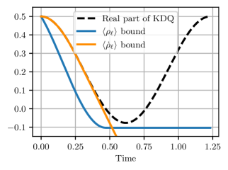
Figure 1: Quasiprobability of a two-qubit system under the conditional-rotation Hamiltonian $\mathcal{H}$ (17). Black line: Real part of KDQ $q_{1,1}$, using $A_{1}=B_{1}=\left\lvert 11\right\rangle\!\left\langle 11\right\rvert$ and initial pure state $\left\lvert-\right\rangle\left\lvert 1\right\rangle$. Negativity is observed choosing $\omega_{L}=1$ and $\omega_{\mathrm{int}}=5$. Blue and orange lines: Lower-bounds to the quasiprobability, both derived from the uncertainty principle. They are respectively obtained by constraining the evolution of $\left\langle\rho_{\ell}\right\rangle$ [Eq. (11)] (blue line) and $\left\langle\dot{\rho}_{\ell}\right\rangle$ [Eq. (12)] (orange line).

Application to conditional gates

​​​— We now show that the maximum power of a work extraction process, which is governed by negativity, can be bounded by an approximated power function computed using the minimal time to negative quasiprobabilities. We do this for the two-qubit controlled-unitary quantum gate experimentally realized in [47]. Such a quantum system evolves according to the time-independent Hamiltonian

$$\mathcal{H}=\frac{\omega_{L}}{2}(Z_{1}+Z_{2})+\frac{\omega_{\mathrm{int}}}{2}{\left\lvert 1\right\rangle\!\left\langle 1\right\rvert\otimes X},$$ (17)

where $Z_{i}$ is the $Z$-Pauli matrix applied to the qubit $i$, $X$ is the $X$-Pauli matrix, and $|0\rangle,|1\rangle$ are respectively the ground and excited states of the local Hamiltonian of each qubit. The first qubit acts as a ‘control’ knob: if it is in the excited state, the second qubit (‘target’) undergoes a rotation of a parameterized angle.

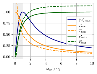
Figure 2: The time to negativity $T_{\mathrm{neg}}$ (dashed orange)—defined as the time at which the bound of $\langle\dot{\rho}_{\ell}\rangle$ in Fig. 1 reaches zero—acts as a lower-bound to the time $T_{\mathrm{max}}$ (solid orange). The latter corresponds to the time when the maximum average work $\langle w\rangle_{\mathrm{max}}$ (blue) is extracted from the target qubit, under the Hamiltonian $\mathcal{H}$ and conditions of Fig. 1. The power at maximum energy extraction, $\mathcal{P}_{\mathrm{max}}=\langle w\rangle_{\mathrm{max}}/T_{\mathrm{max}}$ (solid green), can be well-approximated by the power $\mathcal{P}_{\mathrm{neg}}$ computed at $T_{\mathrm{neg}}$ (dashed green). In fact, $\mathcal{P}_{\mathrm{neg}}$ is an upper-bound of $\mathcal{P}_{\mathrm{max}}$. This reasoning does not apply to the light gray region, where negativity is not observed. The value of the energies, times and powers are respectively normalized by $E_{\mathrm{ref}}=0.5$, $t_{\mathrm{ref}}=\pi$ and $\mathcal{P}_{\mathrm{ref}}\approx 0.32$.

In this process, the internal energy of the target qubit changes with time, as provided by computing the partial trace of the two-qubits state with respect to the control qubit. Since we can manipulate the control qubit at will (even experimentally), the internal energy variation of the target qubit may be interpreted as thermodynamic work exerted by it. We compute the KDQ by setting $A_{\ell}=B_{\ell}=\left\lvert\ell\right\rangle\!\left\langle\ell\right\rvert$ with $\ell=0,1$, meaning that we study work fluctuations originating in local energy measurements.

In this context, preparing the global system in the state $|-\rangle|1\rangle$, where $|-\rangle\equiv(|0\rangle-|1\rangle)/\sqrt{2}$, allows us to observe non-positivity of the computed KDQ. Moreover, here, non-negativity is a signature of extractable work, in a regime where the corresponding value returned by the TPM scheme, $W_{\mathrm{ext}}^{\mathrm{TPM}}\equiv\sum_{\ell,j}(E_{\ell}(t_{1})-E_{j}(t_{2}))p_{\ell,j}^{\mathrm{TPM}}$, is zero for any parameters choice, due to the state-collapse upon the first energy measurement of the TPM scheme.

In Fig. 1 we plot the quasiprobability $\mathrm{Re}\{q_{1,1}\}$, which exhibits negativity, and the lower-bounds (11), (12), for $\omega_{L}=1$ and $\omega_{\mathrm{int}}=5$. For practical purposes, one can take the maximum between the blue and orange curves as the lower-bound to $\mathrm{Re}\{q_{1,1}\}$ for any time $t$. Moreover, in Fig. 2, it shown that the time $T_{\mathrm{neg}}$ for the bound (12) to reach negativity is a lower-bound of the time $T_{\mathrm{max}}$ at which the maximum amount of energy can be possibly extracted from the target qubit. Notably, the work extraction power $\mathcal{P}_{\mathrm{neg}}$ obtained at $T_{\mathrm{neg}}$ turns out to be a pretty good approximation for the power $\mathcal{P}_{\mathrm{max}}$ at $T_{\mathrm{max}}$. Specifically, it is an upper-bound that can be experimentally measured (via local measurements in this example).

Concluding remarks

​​​— We have derived time-dependent bounds for the Kirkwood-Dirac quasiprobabilities, which stems from using the Heisenberg-Robertson uncertainty relation on the time-derivative of the quasiprobabilities. This derivation can be interpreted as a non-commutative extension of the quantum speed limit bound by Mandelstam and Tamm. We have applied our results to determine, from fundamental principles, the minimal time at which a given quasiprobability loses positivity, and to bound the maximum power of a work extraction finite-time process, which is governed by negativity. Consequently, we suggest to further investigate more complex quantum gates [65], and devices for energy conversion [61, 62, 63] including quantum batteries [64].

We conclude by noting that the lower-bound (11) in this Letter is also applicable to operator flows $\mathrm{tr}\left\{\mathcal{O}^{H}\mathcal{O}\right\}$, where $\mathcal{O}$ is any quantum observable [28]. The application of (11) to operator flows relies on the spectral decomposition $\mathcal{O}=\sum_{k}c_{k}\Pi_{k}$, which entails $A_{\ell}=B_{\ell}=\Pi_{\ell}$. On the other hand, the bound in [28] cannot be necessarily used when quasiprobabilities are taken into account, since there are quasiprobabilities that cannot be cast in the form of an operator flow (see the analysis and the counterexample in the SM).