HLbL contributions to $\displaystyle(g-2)_{\mu}$ from axial-vector and tensor mesons in the holographic soft-wall model

Abstract

We compute the axial-vector and tensor meson two-photon transition form factors in the soft-wall holograhic model of QCD. They are used to evaluate the axial-vector and tensor meson contributions to the anomalous magnetic moment of the muon via the hadronic light-by-light scattering process. As expected, these contributions are smaller than the one from pseudoscalar mesons. The result for axial-vector mesons is higher than the value found in other approaches.

1 Introduction

One of the most interesting observables currently under investigation is the anomalous magnetic moment of the muon, $\displaystyle a_{\mu}=(g_{\mu}-2)/2$, which is challenging the Standard Model (SM) of fundamental interactions. The puzzle deals with the current tension between the measurements [1] and a SM prediction [2]. The most precise measurement has been recently provided by the Muon $\displaystyle g-2$ experiment at Fermilab [1], which has improved the precision of the experimental world average by a factor of 2. From the theoretical point of view, a comprehensive prediction for the SM value has been presented in the White Paper of the Muon $\displaystyle g-2$ Theory Initiative in 2020 [2]. The Fermilab result and the expectation quoted in Ref. [2] deviate at a level of about $\displaystyle 5\sigma$. Considering all available data a smaller discrepancy is found [1].

In the SM the largest contribution to $\displaystyle a_{\mu}$ comes from QED processes, and is very precisely known. Electroweak corrections have also been precisely determined [3]. Then, two kinds of QCD contributions are involved: the leading one corresponds to the hadronic vacuum polarization (HVP) [4], the subleading one is due to hadronic light-by-light scattering (HLbL) [5].

QCD contributions are the most interesting to look at, since the theoretical uncertainty is dominated by hadronic effects. A tension exists between the HVP contribution computed from the $\displaystyle e^{+}e^{-}\to hadrons$ cross section data, used in [2], and the lattice QCD result obtained by the BMW collaboration [6]. If the latter value is used to obtain the SM $\displaystyle a_{\mu}$, the discrepancy with the experimental result is reduced to $\displaystyle 1.6\sigma$ [7]. Moreover, there is a discrepancy between the measurements of the $\displaystyle e^{+}e^{-}\to\pi^{+}\pi^{-}$ cross section obtained from the BABAR [8] and KLOE [9] collaborations. In this respect, a recent determination by the CMD-3 collaboration [10] is larger than the previous measurements in the energy range up to $\displaystyle\sqrt{s}\simeq 1.2$ GeV. The latter value would increase the HVP contribution determined in [2], reducing the tension between the experimental value of $\displaystyle a_{\mu}$ and the SM expectation. On the other hand, the confirmation of the discrepancy between experimental and theoretical values of $\displaystyle a_{\mu}$ by forthcoming data and theoretical studies would open exciting perspectives for revealing new-physics effects [11].

The theoretical prediction of the HLbL contribution needs to be improved as well in order to meet the precision of $\displaystyle 16\times 10^{-11}$ for $\displaystyle a_{\mu}$ projected for the Fermilab experiment [12]. The HLbL contribution has been computed in a series of studies summarized in Ref. [2] using a dispersive approach. This allows a model-independent evaluation but fails in reproducing short-distance constraints (SDCs) [13], an issue that has been debated in recent years [14, 15, 16], so a strategy should be found in order to incorporate them. The dominant contribution comes from the poles of the light pseudoscalar mesons. The contributions from other states (scalar, tensor and axial-vector states) are smaller, but need to be computed to improve the theoretical accuracy.

In this paper we compute the axial-vector and tensor meson contributions to the HLbL term in the soft-wall model, a QCD phenomenological holographic approach briefly described in Section 2 [17]. Axial-vector mesons play an essential role since they are expected to solve the SDC puzzle reproducing the correct large-$\displaystyle Q^{2}$ behaviour of the longitudinal four-point function. In this respect, holographic computations in the hard-wall model with different mechanisms of breaking chiral symmetry have proven to be useful in providing an analytical tool for computing the relevant four-point functions, showing how the sum over the infinite tower of axial-vector states can give the expected result [18, 19]. This is discussed in Section 3.

Tensor meson contributions are expected to be smaller than contributions from pseudoscalar exchange. However, in view of improving the theoretical precision it is important to correctly estimate this contribution, for which there are only a few theoretical studies. We compute it by studying the two-photon transition form factor for the helicity-2 meson component in the holographic soft-wall model, obtaining an analytic expression as a function of the photon virtualities. The computation is presented in Section 4, with a few technical details collected in the Appendix.

2 The soft-wall model

The soft-wall (SW) holographic model of QCD is defined in the $\displaystyle 5d$ space with background Anti-de Sitter (AdS) geometry, the bulk, with line element

$$\mathrm{d}s^{2}=g_{MN}\mathrm{d}x^{M}\mathrm{d}x^{N}=\frac{R^{2}}{z^{2}}\left(\eta_{\mu\nu}\mathrm{d}x^{\mu}\mathrm{d}x^{\nu}-\mathrm{d}z^{2}\right)\,.$$ (1)

$\displaystyle R$ is the radius of curvature of the AdS space and $\displaystyle\eta_{\mu\nu}={\rm diag}(1,-1,-1,-1)$. We use Greek letters for Minkowski ($\displaystyle 4d$) indices, and capital letters for AdS ($\displaystyle 5d$) indices. The fifth $\displaystyle z$ (bulk) coordinate runs in the range $\displaystyle\varepsilon<z<\infty$ with $\displaystyle\varepsilon$ a small ($\displaystyle\varepsilon\to 0$) positive UV cutoff. The defining feature of the model is a background (i.e. non-dynamical) dilaton field $\displaystyle\phi(z)$ which only depends on the bulk coordinate $\displaystyle z$ and appears in the Lagrangian as $\displaystyle e^{-\phi(z)}$ [17]. A minimal choice is $\displaystyle\phi(z)=c^{2}z^{2}$, where the dimensionful constant $\displaystyle c$, linked to $\displaystyle\Lambda_{\mathrm{QCD}}$, breaks conformal invariance and is responsible for color confinement. Such a choice for $\displaystyle\phi(z)$ allows to recover linear Regge trajectories for the spectra of light vector mesons [17], light scalar mesons [20], $\displaystyle 0^{++}$ and $\displaystyle 0^{--}$ glueballs [21, 22], and $\displaystyle 1^{-+}$ hybrid mesons [23]. According to the AdS/CFT dictionary, the global $\displaystyle U(n_{f})_{L}\times U(n_{f})_{R}$ symmetry of QCD is dual to a local (gauge) symmetry in the $\displaystyle 5d$ theory, where the fields dual to the QCD left- and right-handed currents $\displaystyle\bar{q}_{L/R}\gamma^{\mu}T^{a}q_{L/R}$ are the massless 1-forms $\displaystyle B_{L}(x,z)$ and $\displaystyle B_{R}(x,z)$. Such gauge fields are expressed as $\displaystyle B^{M}_{\{L,R\}}(x,z)=B^{M,a}_{\{L,R\}}(x,z)T^{a}$, where $\displaystyle T^{a}=\lambda^{a}/2$ ($\displaystyle a=0,...,n_{f}^{2}-1$) are the generators of $\displaystyle U(n_{f})$, with $\displaystyle T^{0}=\frac{1}{\sqrt{2n_{f}}}\mathbb{1}_{n_{f}}$ ($\displaystyle\mathbb{1}_{n_{f}}$ is the $\displaystyle n_{f}\times n_{f}$ identity matrix), and $\displaystyle\mbox{Tr}(T^{a}T^{b})=\delta^{ab}/2$ for $\displaystyle a,b=1,...,n_{f}^{2}-1$. Vector and axial-vector fields are defined as $\displaystyle V=(B_{L}+B_{R})/2$ and $\displaystyle A=(B_{L}-B_{R})/2$, respectively. The $\displaystyle\bar{q}_{R}q_{L}$ operator is dual to a tachyon field $\displaystyle X(x,z)=X_{0}(z)e^{i\pi^{a}(x,z)T^{a}}$, $\displaystyle\pi^{a}$ describing the nonet of pseudoscalar mesons and $\displaystyle X_{0}$ parametrised as $\displaystyle X_{0}(z)=\sqrt{2}v(z)\mathbb{1}_{n_{f}}$. We consider the case of $\displaystyle n_{f}=3$ light quarks. The covariant derivative acts on $\displaystyle X(x,z)$ as

$$\displaystyle D_{M}X=\partial_{M}X+i[X,V_{M}]-i\{X,A_{M}\}\,.$$ (2)

3 Axial-vector meson contribution to $\displaystyle a_{\mu}^{HLbL}$

The quadratic action for the axial-vector field $\displaystyle A_{M}(x,z)$ is [17]

$$S_{A}=\frac{R}{k}\int d^{5}x\,e^{-c^{2}z^{2}}\left(-\frac{1}{4g_{5}^{2}z}F^{a}F^{a}+\frac{4v(z)^{2}}{z^{3}}(A^{a})^{2}\right)\,,$$ (3)

where $\displaystyle F_{MN}=\partial_{M}A_{N}-\partial_{N}A_{M}$. The prefactors $\displaystyle R/k=N_{c}/16\pi^{2}$ and $\displaystyle g_{5}^{2}=3/4$ are fixed by matching the two-point correlation functions of the vector and scalar quark currents to the perturbative QCD expressions [21]. We set the AdS radius $\displaystyle R=1$.

The coupling of the axial field to two vector fields, contributing to $\displaystyle(g-2)_{\mu}$, is provided by the Chern-Simons action [25, 26, 27]

$$S_{CS}=S_{CS}^{L}-S_{CS}^{R}$$ (4)

where

$$S_{CS}^{L/R}=\frac{N_{c}}{24\pi^{2}}\int\,\mbox{Tr}(\mathcal{B}\mathcal{F}^{2})\,,$$ (5)

$\displaystyle\mathcal{B}=B_{M}dx^{M}$ and $\displaystyle\mathcal{F}=(\partial_{A}B_{B})\,dx^{A}\wedge dx^{B}$. In the gauge $\displaystyle B_{z}=0$ and keeping only $\displaystyle VVA$ terms, we find, as in the hard-wall model [19],

$$\displaystyle S_{CS} \displaystyle= \displaystyle-\frac{N_{c}}{6\pi^{2}}\mbox{Tr}(Q_{em}^{2}T^{a})\varepsilon^{\mu\beta\gamma\delta}\int d^{5}x\,(3(\partial_{z}V_{\beta})(\partial_{\gamma}V_{\delta})A_{\mu}^{a}+\partial_{z}(A_{\beta}^{a}(\partial_{\gamma}V_{\delta})V_{\mu}))\,.$$ (6)

$\displaystyle Q_{em}$ is the light-quark electromagnetic charge matrix.

$\displaystyle A_{\mu}$ can be split in a transverse and a longitudinal component: $\displaystyle A_{\mu}^{a}=A^{a\perp}_{\mu}+\partial_{\mu}\varphi^{a}$. The longitudinal component of the axial-vector field $\displaystyle(\varphi^{a})$ mixes with the field $\displaystyle\pi^{a}$ dual to the pseudoscalar current, and they describe psudoscalar mesons. The equations of motion for the transverse and longitudinal components of the axial-vector field come from the quadratic action (3) and in the Fourier space they read:

$$\partial_{z}\left(\frac{e^{-\phi(z)}}{z}\partial_{z}A^{a\perp}_{\mu}(z)\right)+q^{2}\frac{e^{-\phi(z)}}{z}A^{a\perp}_{\mu}(z)-\frac{8g_{5}^{2}v(z)^{2}e^{-\phi(z)}}{z^{3}}A^{a\perp}_{\mu}(z)=0$$ (7)

$$\partial_{z}\left(\frac{e^{-\phi(z)}}{z}\partial_{z}\varphi^{a}(z)\right)+\frac{8g_{5}^{2}v(z)^{2}e^{-\phi(z)}}{z^{3}}(\pi^{a}(z)-\varphi^{a}(z))=0$$ (8)

$$\partial_{z}\left(\frac{e^{-\phi(z)}v(z)^{2}}{z^{3}}\partial_{z}\pi^{a}(z)\right)+\frac{e^{-\phi(z)}v(z)^{2}}{z^{3}}q^{2}(\pi^{a}(z)-\varphi^{a}(z))=0\,.$$ (9)

The eigenvalues $\displaystyle q^{2}=m_{n}^{2}$ for the transverse component are found requiring $\displaystyle A_{n}^{a\perp}(0)=0$ and $\displaystyle\partial_{z}A_{n}^{a\perp}(z)=0$ for $\displaystyle z\to\infty$, and the eigenfunction normalization condition is

$$\frac{R}{kg_{5}^{2}}\int_{0}^{\infty}dz\,\frac{e^{-\phi(z)}}{z}A_{n}^{a\perp}(z)^{2}=1\,.$$ (10)

If we use

$$v(z)=m_{q}z+\sigma z^{3}\,,$$ (11)

with $\displaystyle m_{q}=3.47$ MeV, $\displaystyle\sigma=0.149$ GeV³ and $\displaystyle c=0.388$ GeV, fixed from the pion mass, the pion decay constant and the $\displaystyle\rho$ mass [27], respectively, we find $\displaystyle m_{0}=1.679$ GeV for the ground-state mass. The axial-vector decay constant, defined as

$$\langle 0|\bar{q}\gamma_{\mu}\gamma_{5}T^{a}q|A_{n}\rangle=f_{n}^{a}m_{n}\varepsilon_{\mu}\,,$$ (12)

can be computed from

$$f_{n}^{a}=\frac{R}{kg_{5}^{2}}\frac{1}{m_{n}}\lim_{z\to 0}\frac{e^{-\phi(z)}}{z}\partial_{z}A_{n}^{a\perp}(z)\,.$$ (13)

For the ground state we find $\displaystyle f_{0}^{a}=221$ MeV. These results are independent of the flavour index $\displaystyle a$.

The contribution to muon $\displaystyle g-2$ from the longitudinal component of the axial-vector field in the soft-wall model has been analysed in [27], where the $\displaystyle\eta^{\prime}$ meson has been included considering the mixing between pseudoscalar mesons and pseudoscalar glueballs [28].

Let us compute the contribution of axial-vector mesons (transverse component) to the correlation function of four vector currents, the $\displaystyle\Pi^{A}_{\mu\nu\lambda\sigma}$ tensor. As in Ref. [19], we consider it as the sum of the product of two three-point amplitudes times a propagator over all intermediate axial-vector states [29]:

$$\displaystyle\Pi^{A}_{\mu\nu\lambda\sigma}(q_{1},q_{2},q_{3},q_{4}) \displaystyle= \displaystyle M_{\mu\nu\alpha}(q_{1},q_{2})\frac{iP^{\alpha\beta}(q_{3}+q_{4})}{(q_{3}+q_{4})^{2}-M_{A}^{2}}M_{\lambda\sigma\beta}(q_{3},q_{4})$$ (14)

$$\displaystyle+ \displaystyle M_{\mu\sigma\alpha}(q_{1},q_{4})\frac{iP^{\alpha\beta}(q_{1}+q_{4})}{(q_{1}+q_{4})^{2}-M_{A}^{2}}M_{\nu\lambda\beta}(q_{2},q_{3})$$

$$\displaystyle+ \displaystyle M_{\mu\lambda\alpha}(q_{1},q_{3})\frac{iP^{\alpha\beta}(q_{1}+q_{3})}{(q_{1}+q_{3})^{2}-M_{A}^{2}}M_{\nu\sigma\beta}(q_{2},q_{4})\,,$$

where $\displaystyle M_{A}$ is the mass of the axial-vector meson, $\displaystyle P_{\mu\nu}=\eta_{\mu\nu}-\frac{q_{\mu}q_{\nu}}{M_{A}^{2}}$ is the projector for spin 1 mesons, and $\displaystyle q_{1},q_{2},q_{3},q_{4}$ are the momenta of the incoming photons.

The amplitude $\displaystyle\gamma^{*}\gamma^{*}\to A_{n}^{a}$ can be written as [19, 29]

$$M_{\mu\nu\alpha}(q_{1},q_{2})=e^{2}\varepsilon_{\rho\nu\alpha\tau}(q_{1}^{2}g_{\mu}^{\rho}-q_{1}^{\rho}q_{1\mu})q_{2}^{\tau}F_{A\gamma^{*}\gamma^{*}}(q_{1}^{2},q_{2}^{2})-e^{2}\varepsilon_{\mu\rho\alpha\tau}(q_{2}^{2}g_{\nu}^{\rho}-q_{2}^{\rho}q_{2\nu})q_{1}^{\tau}F_{A\gamma^{*}\gamma^{*}}(q_{2}^{2},q_{1}^{2})$$ (15)

where $\displaystyle F_{A\gamma^{*}\gamma^{*}}$ is the two-photon transition form factor (TFF). In the soft-wall model the three-point function of an axial-vector current and two vector currents is obtained from the Chern-Simons action (6), and the TFF of the axial-vector meson $\displaystyle A_{n}^{a\perp}$ to two photons is given by [19]:

$$F_{A^{a}_{n}\gamma^{*}\gamma^{*}}(Q_{1}^{2},Q_{2}^{2})=\frac{N_{c}}{4\pi^{2}}\mbox{Tr}(Q_{em}^{2}T^{a})\frac{2}{Q_{1}^{2}}\int_{0}^{\infty}dz\,A_{n}^{a\perp}(z)\,\partial_{z}V(z,Q_{1}^{2})\,V(z,Q_{2}^{2})\,,$$ (16)

where $\displaystyle Q_{i}^{2}=-q_{i}^{2}$ and $\displaystyle V(z,Q^{2})$ is the bulk-to-boundary propagator (BTBP) of the vector field

$$V(z,Q^{2})=\frac{Q^{2}}{4c^{2}}\,\Gamma\left(\frac{Q^{2}}{4c^{2}}\right)\,U\left(\frac{Q^{2}}{4c^{2}},0,c^{2}z^{2}\right)\,,$$ (17)

with $\displaystyle U$ the Tricomi confluent hypergeometric function [17, 26]. In the model the light quark masses coincide and we do not distinguish among mesons with $\displaystyle a=3,8,0$. In the TFF the only difference between the states is in the factor $\displaystyle\mbox{Tr}(Q_{em}^{2}T^{a})$. We find that the form factors of the lowest-lying axial-vector mesons with $\displaystyle a=8,0$ to one small-$\displaystyle q^{2}$ longitudinal photon and one real transverse photon are $\displaystyle F_{A^{8}_{0}\gamma\gamma}=-0.170\mbox{ GeV}^{-2}$ and $\displaystyle F_{A^{0}_{0}\gamma\gamma}=-0.480\mbox{ GeV}^{-2}$. The boundary values of the axial-vector eigenfunctions in the soft-wall model guarantee that the amplitude for the decay in two real photons vanishes, satisfying the Landau-Yang theorem. An equivalent two-photon decay width for an axial-vector meson to decay in one quasi-real longitudinal photon and a real photon can be defined as [30]

$$\tilde{\Gamma}_{A_{0}^{a}\to\gamma\gamma}=\lim_{Q_{1}^{2}\to 0}\frac{m_{0}^{2}}{Q_{1}^{2}}\frac{1}{2}\Gamma_{A_{0}^{a}\to\gamma^{*}\gamma}=\frac{\pi\alpha^{2}m_{0}^{5}}{12}F_{A^{a}_{0}\gamma\gamma}^{2}\,,$$ (18)

where $\displaystyle Q_{1}^{2}$ is the virtuality of the photon $\displaystyle\gamma^{*}$. We find $\displaystyle\tilde{\Gamma}_{A_{0}^{8}\gamma\gamma}=5.4$ keV and $\displaystyle\tilde{\Gamma}_{A_{0}^{0}\gamma\gamma}=43$ keV. In the hard-wall (HW) model $\displaystyle F_{A^{8}_{0}\gamma\gamma}=-0.154\mbox{ GeV}^{-2}$ and $\displaystyle F_{A^{0}_{0}\gamma\gamma}=-0.435\mbox{ GeV}^{-2}$ have been found [19]. Experimental data for $\displaystyle f_{1}(1285)$ and $\displaystyle f_{1}(1420)$ are: $\displaystyle\tilde{\Gamma}_{\gamma\gamma}=3.5(8)$ keV for $\displaystyle f_{1}(1285)$ [31] and $\displaystyle\tilde{\Gamma}_{\gamma\gamma}=3.2(9)$ keV for $\displaystyle f_{1}(1420)$ [32].

Fig. 1 shows the $\displaystyle Q^{2}$ dependence of the axial-vector TFF with one real photon compared to the result in the hard-wall model [19] and to the dipole parametrization of Ref. [29]

$$\frac{F_{A\gamma\gamma}(Q_{1}^{2},Q_{2}^{2})}{F_{A\gamma\gamma}(0,0)}=\frac{1}{(1+Q_{1}^{2}/\Lambda^{2})^{2}}\frac{1}{(1+Q_{2}^{2}/\Lambda^{2})^{2}}$$ (19)

with $\displaystyle\Lambda=1040\pm 78$ MeV determined from phenomenology for $\displaystyle f_{1}(1285)$ [31]. A similar plot is shown in Fig. 2 for $\displaystyle F_{A^{a}_{0}\gamma^{*}\gamma^{*}}(Q^{2},Q^{2})$. The high-$\displaystyle Q^{2}$ behaviour in the holographic models is the same as in the dipole parametrization for the TFF with one real photon. For two virtual photons the holographic models still find a $\displaystyle Q^{-4}$ decrease of the TFF, while the parametrization in [29] produces a $\displaystyle Q^{-8}$ decrease. As noticed in [19, 33], defining $\displaystyle Q^{2}=(Q_{1}^{2}+Q_{2}^{2})/2$ and $\displaystyle w=(Q_{1}^{2}-Q_{2}^{2})/(Q_{1}^{2}+Q_{2}^{2})$, the asymptotic behaviour of the axial-vector TFF for $\displaystyle Q^{2}\to\infty$ in both the soft-wall and hard-wall models is:

$$\displaystyle F_{A^{a}_{0}\gamma^{*}\gamma^{*}}(Q_{1}^{2},Q_{2}^{2}) \displaystyle\xrightarrow[Q^{2}\to\infty]{} \displaystyle-N_{c}\mbox{Tr}(Q_{em}^{2}T^{a})\frac{f_{0}^{a}m_{0}}{Q^{4}}\sqrt{1-w}\int_{0}^{\infty}dx\,x^{4}\,K_{0}(x\sqrt{1+w})\,K_{1}(x\sqrt{1-w})$$

$$\displaystyle= \displaystyle-N_{c}\mbox{Tr}(Q_{em}^{2}T^{a})\frac{f_{0}^{a}m_{0}}{Q^{4}w^{4}}\left(w(3-2w)+\frac{1}{2}(w+3)(1-w)\log\frac{1-w}{1+w}\right)\,,$$

a result which agrees with the expansion in [34]. $\displaystyle K_{n}(x)$ is the modified Bessel function of the second kind. The hard-wall and soft-wall models give the same result in this limit since the leading behaviour of vector meson BTBP in both models is $\displaystyle V(z,Q^{2})=z\sqrt{Q^{2}}K_{1}(z\sqrt{Q^{2}})$ [26]. To obtain Eq. (3) we have used the expansion of the axial wavefunction at small $\displaystyle z$ and the definition of the axial-vector decay constant $\displaystyle f_{0}^{a}$ in (13):

$$A_{0}^{a\perp}(z)\xrightarrow[z\to 0]{}\left(\frac{R}{kg_{5}^{2}}\right)^{-1}\frac{f_{0}^{a}m_{0}}{2}z^{2}\,.$$ (21)

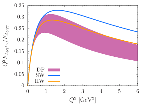
Figure 1: Axial-vector two-photon transition form factor for one real photon. The blue curve shows the result obtained in the soft-wall model (SW); the orange curve shows the result obtained in the hard-wall model (HW) [19]; the magenta band shows the dipole-parametrization expression (DP) in Eq. (19) including the uncertainty on the parameter $\displaystyle\Lambda$.

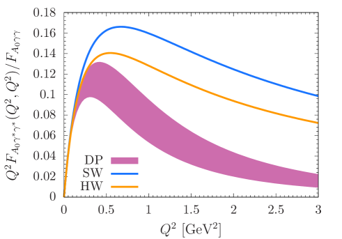
Figure 2: Axial-vector transition form factor for two virtual photons. Line colors are the same as in Fig. 1.

The hadronic light-by-light (HLbL) pole contribution from axial-vector mesons to $\displaystyle(g-2)_{\mu}$ can be computed from

$$a_{\mu}^{HLbL}=\int_{0}^{\infty}dQ_{1}\int_{0}^{\infty}dQ_{2}\int_{-1}^{1}d\tau\,\rho_{a}(Q_{1},Q_{2},\tau)\,,$$ (22)

where $\displaystyle\rho_{a}$ is defined in the appendix of Ref. [19]. We find $\displaystyle a^{HLbL}_{\mu,A^{3}}=9.0\times 10^{-11}$, $\displaystyle a^{HLbL}_{\mu,A^{8}}=3.0\times 10^{-11}$, $\displaystyle a^{HLbL}_{\mu,A^{0}}=2.4\times 10^{-10}$ (the difference is only due to the factor $\displaystyle\mbox{Tr}(Q_{em}^{2}T^{a})$), the sum being $\displaystyle a^{HLbL}_{\mu}=3.6\times 10^{-10}$. In Table 1 other determinations are collected, showing that a large uncertainty affects the size of this contribution. The soft-wall model, as well as the hard-wall model [19], points towards high values. Indeed, it has been noticed [13, 14] that higher $\displaystyle a_{\mu}$ from axial-vector mesons are found in models able to reproduce the SDCs on the longitudinal four-point function.

Ref.	$\displaystyle a_{1}^{0}$	$\displaystyle f_{1}(1285)$	$\displaystyle f_{1}^{\prime}(1420)$	Sum
[2]				6 $\displaystyle\pm$ 6
[35]				2.5 $\displaystyle\pm$ 1
[36]				1.738 $\displaystyle\pm$ 0.003
[13]	5.7	15.6	0.8	22 $\displaystyle\pm$ 5
[29]		5.0$\displaystyle\pm$2.0	1.4$\displaystyle\pm$0.7	6.4$\displaystyle\pm$ 2.0
[37]	0.21$\displaystyle\pm$0.04	0.58$\displaystyle\pm$0.11	0.015$\displaystyle\pm$0.008	0.8${}^{+3.5}_{-0.8}$
[14]	5.89	10.52	1.97	18.38
[38]				3.6$\displaystyle\pm$1.8
[18]	8	8	12	28
[39]				27.8
This work				36

Table 1: HLbL contribution to $\displaystyle a_{\mu}$ ($\displaystyle\times 10^{11}$) of the axial-vector mesons $\displaystyle a_{1},f_{1},f_{1}^{\prime}$ in the indicated models. For more results see Table 13 in [2]. In Ref. [18] the result corresponds to the whole meson tower.

Notice that, as stated in Ref. [29], when calculating $\displaystyle a^{HLbL}_{\mu}$ the sum over polarizations of spin-1 particles gives the projector $\displaystyle P_{\mu\nu}=\eta_{\mu\nu}-\frac{q_{\mu}q_{\nu}}{M_{A}^{2}}$, containing both transverse and longitudinal contributions. We can separate them as the sum of a transverse $\displaystyle P^{\perp}_{\mu\nu}=\eta_{\mu\nu}-\frac{q_{\mu}q_{\nu}}{q^{2}}$ and a longitudinal projector $\displaystyle P^{||}_{\mu\nu}=\frac{q_{\mu}q_{\nu}}{q^{2}}\frac{M_{A}^{2}-q^{2}}{M_{A}^{2}}$. Using the transverse projector we find $\displaystyle a^{HLbL,\perp}_{\mu}=1.5\times 10^{-10}$, using the longitudinal one we find $\displaystyle a^{HLbL,||}_{\mu}=1.8\times 10^{-10}$, both values include the contributions from $\displaystyle a=3,8,0$.

Let us conclude this Section with a comment on the SDCs. The longitudinal component of the HLbL four-point function can be expressed as

$$\Pi_{\mu\nu\alpha\beta}^{||}(q_{1},q_{2},q_{3},q_{4})=T^{(1)}_{\mu\nu\alpha\beta}\bar{\Pi}_{1}+T^{(2)}_{\mu\nu\alpha\beta}\bar{\Pi}_{2}+T^{(3)}_{\mu\nu\alpha\beta}\bar{\Pi}_{3}$$ (23)

with $\displaystyle T^{(1)}_{\mu\nu\alpha\beta}=\varepsilon_{\mu\nu\rho\sigma}\varepsilon_{\alpha\beta\rho^{\prime}\sigma^{\prime}}q_{1}^{\rho}q_{2}^{\sigma}q_{3}^{\rho^{\prime}}q_{4}^{\sigma^{\prime}}$, and $\displaystyle T^{(2,3)}$ and $\displaystyle\bar{\Pi}_{2,3}$ obtained by crossing operations [18]. The SDC conditions are [13]:

$$\displaystyle\lim_{Q_{3}\to\infty}\lim_{Q\to\infty}Q^{2}Q_{3}^{2}\bar{\Pi}_{1}(Q,Q,Q_{3})=-\frac{2}{3\pi^{2}}$$ (24)

$$\displaystyle\lim_{Q\to\infty}Q^{4}\bar{\Pi}_{1}(Q,Q,Q)=-\frac{4}{9\pi^{2}}\,.$$ (25)

They have been checked in the hard-wall model in Ref. [19, 33] and they are also obtained in the soft-wall model and agree with the considerations of Ref. [14]. The factorized contribution from pions scales as $\displaystyle 1/Q^{6}$, of higher order in the $\displaystyle Q^{2}\to\infty$ expansion than the result from the OPE. The longitudinal contribution from axial-vector mesons (obtained from the projector $\displaystyle\frac{q_{\mu}q_{\nu}}{q^{2}}\frac{M_{A}^{2}-q^{2}}{M_{A}^{2}}$) is instead of the same order than the OPE result: it matches the OPE result in the region $\displaystyle Q^{2}_{1}\sim Q^{2}_{2}\gg Q^{2}_{3}\gg m^{2}_{\rho}$, while in the region $\displaystyle Q^{2}_{1}=Q^{2}_{2}=Q^{2}_{3}\gg m^{2}_{\rho}$ the correct power behaviour is reproduced although the numerical factor is slightly smaller:

$$\lim_{Q\to\infty}Q^{4}\bar{\Pi}_{1}(Q,Q,Q)\sim-\frac{0.36}{\pi^{2}}\,.$$ (26)

4 Tensor meson contribution to $\displaystyle a_{\mu}^{HLbL}$

Tensor mesons with $\displaystyle J^{PC}=2^{++}$ can be described in holographic models by a field dual to the $\displaystyle j_{\mu\nu}=\bar{q}\frac{1}{2}\left(\gamma_{\mu}i\overleftrightarrow{D}_{\nu}-\gamma_{\nu}i\overleftrightarrow{D}_{\mu}\right)q$ operator, i.e. by a massless 2-form [40]. In [41] the spin-2 traceless field $\displaystyle h_{\mu\nu}$ (graviton) is introduced as the 4$\displaystyle d$ fluctuation of the metric (1):

$$ds^{2}=g_{MN}dx^{M}dx^{N}=\frac{1}{z^{2}}(\eta_{\mu\nu}+h_{\mu\nu})dx^{\mu}dx^{\nu}-\frac{1}{z^{2}}dz^{2}\,.$$ (27)

This field has helicity $\displaystyle\pm 2$. The quadratic action in the soft-wall model is

$$S=-k_{T}\int d^{5}x\sqrt{g}\,e^{-\phi}\mathcal{R}=-\frac{k_{T}}{2}\int d^{5}x\frac{e^{-\phi}}{z^{3}}\eta^{\mu\alpha}\eta^{\nu\beta}(\partial_{z}h_{\mu\nu}\partial_{z}h_{\alpha\beta}-h_{\mu\nu}\Box h_{\alpha\beta})\,,$$ (28)

where $\displaystyle\mathcal{R}$ is the Ricci scalar. The same action can be obtained starting from the action of a rank-2 symmetric tensor field $\displaystyle H_{AB}$:

$$S_{2}\propto\frac{1}{2}\int d^{5}x\sqrt{g}\,e^{-\phi}\nabla_{M}H_{AB}\nabla^{M}H^{AB}$$ (29)

assuming $\displaystyle H_{Az}=0$, $\displaystyle\partial^{\mu}H_{\mu\nu}=0$, $\displaystyle H_{\mu\nu}=h_{\mu\nu}/z^{2}$, removing boundary terms and the $\displaystyle h_{\mu\nu}^{2}$ term. From the action (28), the equation of motion in the Fourier space is

$$\partial_{z}\left(\frac{e^{-\phi}}{z^{3}}\partial_{z}h_{\mu\nu}\right)+\frac{e^{-\phi}}{z^{3}}q^{2}h_{\mu\nu}=0\,.$$ (30)

The two-point correlation function is found from the on-shell action:

$$S_{os}=\lim_{z\to 0}\frac{k_{T}}{2}\int d^{4}x\frac{e^{-\phi}}{z^{3}}\eta^{\mu\alpha}\eta^{\nu\beta}h_{\mu\nu}\partial_{z}h_{\alpha\beta}$$ (31)

deriving it with respect to the sources of the $\displaystyle 4d$ tensor operator [42]. In the Fourier space the field $\displaystyle h_{\mu\nu}$ is related to the source $\displaystyle h_{0\mu\nu}$ by: $\displaystyle h_{\mu\nu}(z,q^{2})=h_{B}(z,q^{2})h_{0\mu\nu}(q^{2})$, where $\displaystyle h_{B}$ is the bulk-to-boundary propagator

$$h_{B}(z,q^{2})=\Gamma\left(2-\frac{q^{2}}{4c^{2}}\right)U\left(-\frac{q^{2}}{4c^{2}},-1,c^{2}z^{2}\right)\,$$ (32)

obtained by solving the equation of motion (30) with boundary conditions $\displaystyle h_{B}(0,q^{2})=1$ and finiteness of the action. The two-point function reads

$$\Pi^{\mu\nu\rho\sigma}=\frac{\delta^{2}S_{os}}{\delta h_{0\mu\nu}\delta h_{0\rho\sigma}}=k_{T}P^{\mu\nu\rho\sigma}\lim_{z\to 0}\frac{e^{-\phi}}{z^{3}}h_{B}\partial_{z}h_{B}\,,$$ (33)

where $\displaystyle P_{\mu\nu\rho\sigma}=\frac{1}{2}(\eta_{\mu\rho}\eta_{\nu\sigma}+\eta_{\mu\sigma}\eta_{\nu\rho}-\frac{2}{3}\eta_{\mu\nu}\eta_{\rho\sigma})$ is the transverse projector. For $\displaystyle Q^{2}=-q^{2}\to\infty$ one has ($\displaystyle\nu$ is an energy scale)

$$\Pi^{\mu\nu\rho\sigma}\to-k_{T}P^{\mu\nu\rho\sigma}\frac{Q^{4}}{8}\log(Q^{2}/\nu^{2})$$ (34)

to be compared with [41, 43]

$$\Pi^{\mu\nu\rho\sigma}_{QCD}\to-P^{\mu\nu\rho\sigma}\left(\frac{N_{c}N_{f}}{160\pi^{2}}+\frac{N_{c}^{2}-1}{80\pi^{2}}\right)Q^{4}\log(Q^{2}/\nu^{2})\,.$$ (35)

This condition fixes $\displaystyle k_{T}=\left(\frac{N_{c}N_{f}}{20\pi^{2}}+\frac{N_{c}^{2}-1}{10\pi^{2}}\right)$.

Eigenvalues and eigenfunctions are found by solving Eq. (30) requiring $\displaystyle h_{n}(0)=0$ and normalisation

$$\int_{0}^{\infty}dz\,\frac{e^{-\phi(z)}}{z^{3}}h_{n}(z)^{2}=1\,.$$ (36)

The spectrum is $\displaystyle m_{n}^{2}=4c^{2}(n+2)$ and the wavefunctions are:

$$h_{n}(z)=\sqrt{\frac{2}{(n+1)(n+2)}}\,c^{3}z^{4}\,L_{n}^{2}(c^{2}z^{2}).$$ (37)

The residues of the poles of the two-point function are $\displaystyle R_{n}=k_{T}8c^{6}(n+1)(n+2)$. From $\displaystyle R_{n}=f_{n}^{2}m_{n}^{4}$ we find the decay constants $\displaystyle f_{n}=c\sqrt{k_{T}(n+1)/(2(n+2))}$. For $\displaystyle c=0.388$ GeV we obtain $\displaystyle m_{f_{2}}=1.097$ GeV and $\displaystyle f_{f_{2}}=69$ MeV (corresponding to $\displaystyle n=0$), while the first excitation ($\displaystyle n=1$) has mass $\displaystyle m_{1}=1.344$ GeV and decay constant $\displaystyle f_{1}=80$ MeV. The decay constant $\displaystyle g_{f}=f_{f_{2}}/m_{f_{2}}=\sqrt{5/2}/(8\pi)=0.063$ can be compared to Ref. [44] where $\displaystyle g_{f}=0.040$ is found, while in the hard-wall model one has $\displaystyle g_{f}=0.024$ [41].

The decay $\displaystyle f_{2}\to\gamma^{*}\gamma^{*}$ can be studied from the quadratic action of the vector field considering the fluctuation of the metric:

$$\displaystyle S_{f_{2}\gamma\gamma} \displaystyle\supset \displaystyle-\frac{R}{2kg_{5}^{2}}\int d^{5}x\sqrt{g}e^{-\phi}\mbox{Tr}(F_{MN}F^{MN})$$ (38)

with $\displaystyle F_{MN}=\partial_{M}V_{N}-\partial_{N}V_{M}$. In the Fourier space, after introducing the source $\displaystyle V_{\alpha}(q)$ and the BTBP $\displaystyle V(z,q)$ (17) of the vector field, we find:

$$\displaystyle S_{f_{2}\gamma\gamma} \displaystyle\propto \displaystyle\int d^{4}q_{1}\int d^{4}q_{2}\int\frac{dz}{z}e^{-\phi}h_{\alpha\beta}(z,q_{1}+q_{2})V_{\mu}(q_{1})V_{\nu}(q_{2})$$ (39)

$$\displaystyle(-\eta^{\mu\alpha}\eta^{\nu\beta}\partial_{z}V(z,q_{1})\partial_{z}V(z,q_{2})$$

$$\displaystyle+(q_{1}\cdot q_{2}\eta^{\mu\alpha}\eta^{\nu\beta}-q_{1}^{\alpha}q_{2}^{\mu}\eta^{\nu\beta}+q_{1}^{\alpha}q_{2}^{\beta}\eta^{\mu\nu}-q_{1}^{\nu}q_{2}^{\beta}\eta^{\mu\alpha})V(z,q_{1})V(z,q_{2}))\,.$$

To find the amplitude, we derive the action with respect to the three sources of the fields and write the BTBP of the tensor field as the sum

$$h(z,q^{2})=\sum_{n}\frac{h_{n}(z)\sqrt{R_{n}/k_{T}}}{-q^{2}+m_{n}^{2}}\,.$$ (40)

The amplitude for $\displaystyle f_{2}\to\gamma^{*}\gamma^{*}$ is

$$\displaystyle\mathcal{M}_{\mu\nu\alpha\beta} \displaystyle= \displaystyle A_{f_{2}}\,(q_{1}\cdot q_{2}\,\eta_{\mu\alpha}\eta_{\nu\beta}-q_{1\alpha}\,q_{2\mu}\,\eta_{\nu\beta}+q_{1\alpha}\,q_{2\beta}\,\eta_{\mu\nu}-q_{1\nu}\,q_{2\beta}\,\eta_{\mu\alpha})$$ (41)

$$\displaystyle\int_{0}^{\infty}\frac{dz}{z}e^{-\phi}h_{0}(z)\left(-\frac{1}{q_{1}\cdot q_{2}}\partial_{z}V(z,q_{1})\partial_{z}V(z,q_{2})+V(z,q_{1})V(z,q_{2})\right)\,,$$

where we have introduced the parameter $\displaystyle A_{f_{2}}$. The amplitude in (41) has the same Lorentz structure given in [45]. In [29] a different form has been proposed for the amplitude. We have checked that the $\displaystyle f_{2}$ contribution to muon $\displaystyle g-2$ gets similar values if $\displaystyle a_{\mu}^{HLbL}$ is computed using the amplitude in [45] or in [29]. From Eq. (41) the two-photon transition form factor can be extracted ($\displaystyle q_{i}^{2}=-Q_{i}^{2}$):

$$\displaystyle\mathcal{F}_{f_{2}\gamma^{*}\gamma^{*}}(Q_{1}^{2},Q_{2}^{2}) \displaystyle= \displaystyle A_{f_{2}}\int_{0}^{\infty}\frac{dz}{z}e^{-\phi}h_{0}(z)$$ (42)

$$\displaystyle\left(\frac{-2}{m_{0}^{2}+Q_{1}^{2}+Q_{2}^{2}}\partial_{z}V(z,Q_{1}^{2})\partial_{z}V(z,Q_{2}^{2})+V(z,Q_{1}^{2})V(z,Q_{2}^{2})\right)\,.$$

Eq. (42) can also be used to compute the TFF in the hard-wall model with some modifications: the upper limit of the integral is $\displaystyle z_{0}=(322\mbox{ MeV})^{-1}$, the dilaton vanishes, the tensor wavefunction is [41]

$$h_{0}^{HW}(z)=3.51\frac{z^{2}}{z_{0}}J_{2}(m_{0}\,z)$$ (43)

with the tensor mass $\displaystyle m_{0}=1.23$ GeV, the vector BTBP is [19]

$$V^{HW}(z,Q^{2})=\sqrt{Q^{2}}z\left(K_{1}(\sqrt{Q^{2}}z)+I_{1}(\sqrt{Q^{2}}z)\frac{K_{0}(\sqrt{Q^{2}}z_{0})}{I_{0}(\sqrt{Q^{2}}z_{0})}\right)\,.$$ (44)

If one photon is real, only the second term in (42) contributes to $\displaystyle\mathcal{F}_{f_{2}\gamma^{*}\gamma}$, and its behaviour in the soft-wall and hard-wall models is shown in Fig. 3 together with data for the helicity-2 component of $\displaystyle f_{2}(1270)$ from Belle collaboration [46]. The curve obtained in the hard-wall model has a better agreement with the experimental points, and this is due to the fact that the ground-state mass prediction of the HW is closer to the experimental $\displaystyle f_{2}(1270)$ mass than the SW prediction. Indeed, if the $\displaystyle f_{2}(1270)$ mass is used to fix the mass scale $\displaystyle c$ in the soft-wall model, the TFF in the SW and HW models are similar. In Fig. 4 the results from [47] and two determinations from [30] are also shown. In Fig. 5 $\displaystyle\mathcal{F}_{f_{2}\gamma^{*}\gamma^{*}}(Q^{2},Q^{2})$ for two photons with equal virtualities is shown.

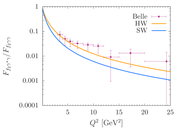
Figure 3: $\displaystyle f_{2}$ TFF with one real and one virtual photon in the soft-wall (blue curve) and hard-wall (orange curve) models. Belle data are from Ref. [46].

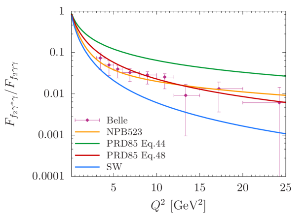
Figure 4: $\displaystyle f_{2}$ TFF with one real and one virtual photon in the soft-wall model (blue curve), compared with results found in other models: Ref. [47] (orange curve), [30] (green and red curves). Belle data are from Ref. [46].

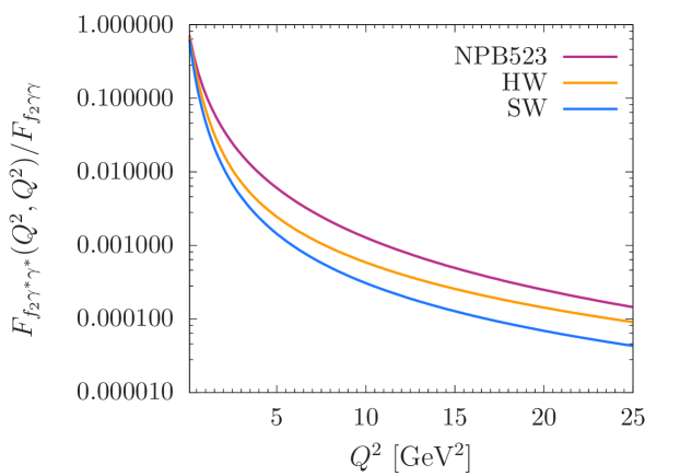
Figure 5: $\displaystyle f_{2}$ TFF with two virtual photons in the soft-wall model (blue curve), hard-wall (orange curve) model and computed in Ref. [47] (magenta curve).

The $\displaystyle f_{2}(1270)\to\gamma\gamma$ decay width is $\displaystyle\Gamma_{\gamma\gamma}=2.6\pm 0.5$ keV [48], and it is related to the form factor by

$$\Gamma_{\gamma\gamma}=\frac{\pi\alpha^{2}}{20}m_{0}^{3}\mathcal{F}_{f_{2}\gamma\gamma}^{2}\,,$$ (45)

which fixes $\displaystyle\mathcal{F}_{f_{2}\gamma\gamma}=0.387$ GeV^-1. From Eq. (42) we find that for two real photons $\displaystyle\mathcal{F}_{f_{2}\gamma\gamma}=A_{f_{2}}/2c$ in the soft-wall model, so we fix $\displaystyle A_{f_{2}}=0.3$, while in the hard-wall model $\displaystyle A_{f_{2}}=0.186$.

As done for axial-vector mesons, the asymptotic large-$\displaystyle Q^{2}$ behaviour of the $\displaystyle f_{2}$ TFF can be analytically obtained from Eq. (42) defining the variables $\displaystyle Q^{2}=(Q_{1}^{2}+Q_{2}^{2})/2$ and $\displaystyle w=(Q_{1}^{2}-Q_{2}^{2})/(Q_{1}^{2}+Q_{2}^{2})$, noticing that in the soft-wall model $\displaystyle V(z,Q^{2})\xrightarrow[Q^{2}\to\infty]{}z\sqrt{Q^{2}}K_{1}(z\sqrt{Q^{2}})$ [26] and $\displaystyle h_{0}(z)=f_{0}m_{0}^{2}/(4\sqrt{k_{T}})z^{4}$. We find:

$$\displaystyle F_{f_{2}\gamma^{*}\gamma^{*}} \displaystyle\xrightarrow[Q^{2}\to\infty]{} \displaystyle A_{f_{2}}\frac{f_{0}m_{0}^{2}}{4\sqrt{k_{T}}Q^{4}}\int_{0}^{\infty}dx\,x^{5}$$

$$\displaystyle[-(1-w^{2})K_{0}(x\sqrt{1+w})\,K_{0}(x\sqrt{1-w})+\sqrt{1-w^{2}}K_{1}(x\sqrt{1+w})\,K_{1}(x\sqrt{1-w})]$$

$$\displaystyle= \displaystyle\frac{F_{f_{2}\gamma\gamma}}{4\sqrt{2k_{T}}}\frac{f_{0}m_{0}^{3}}{Q^{4}w^{5}}\left(4w(6-5w^{2})+2(6-7w^{2}+w^{4})\log\frac{1-w}{1+w}\right)\,.$$

The expansion in [34] has the same $\displaystyle Q^{2}$ but a different $\displaystyle w$ behaviour.

The results for the TFF can be used to compute the HLbL pole contribution of tensor mesons to muon $\displaystyle g-2$ using Eq. (55) in the Appendix. We find that the $\displaystyle f_{2}(1270)$ contribution to muon $\displaystyle g-2$ is $\displaystyle a^{HLbL}_{\mu}\sim 0.61\times 10^{-11}$ in the soft-wall model and $\displaystyle a^{HLbL}_{\mu}\sim 0.63\times 10^{-11}$ in the hard-wall model. They agree with the result in [29] $\displaystyle a^{HLbL}_{\mu}=(0.79\pm 0.09)\times 10^{-11}$. In Ref. [49] $\displaystyle a^{HLbL}_{\mu}=(0.50\pm 0.13)\times 10^{-11}$ and $\displaystyle a^{HLbL}_{\mu}=(0.21\pm 0.05)\times 10^{-11}$ are obtained for $\displaystyle f_{2}(1270)$ and $\displaystyle f_{2}(1565)$, respectively.

5 Conclusions

Holographic bottom-up models, despite their simplicity, provide a good description of QCD observables. This also holds for the two-photon transition form factors of axial-vector and tensor mesons. The TFF of tensor mesons in the soft-wall model is smaller than experimental values but the differences are within the experimental errors. A better agreement is found between the hard-wall model and experimental data, since the mass prediction better reproduces the measured $\displaystyle f_{2}(1270)$ mass. The results for axial-vector and tensor meson contributions to the anomalous magnetic moment of the muon confirm the decreasing hierarchy from pseudoscalar, axial-vector and tensor meson poles. The values we have found in the soft-wall model are $\displaystyle a_{\mu}^{HLbL}=3.6\times 10^{-10}$ for axial-vector mesons and $\displaystyle a_{\mu}^{HLbL}=0.61\times 10^{-11}$ for tensor mesons.

Appendix A $\displaystyle a^{HLbL}_{\mu}$ from tensor meson poles

The HLbL contribution to the anomalous magnetic moment of the muon is computed from [3]:

$$\displaystyle a^{HLbL}_{\mu} \displaystyle= \displaystyle-\frac{ie^{6}}{48m_{\mu}}\int\frac{d^{4}q_{1}}{(2\pi)^{4}}\int\frac{d^{4}q_{2}}{(2\pi)^{4}}\frac{1}{q_{1}^{2}q_{2}^{2}(k-q_{1}-q_{2})^{2}}\frac{1}{(p-q_{1})^{2}-m_{\mu}^{2}}\frac{1}{(p-q_{1}-q_{2})^{2}-m_{\mu}^{2}}$$ (47)

$$\displaystyle\mbox{Tr}\left((\not{p}+m_{\mu})[\gamma^{\rho},\gamma^{\sigma}](\not{p}+m_{\mu})\gamma^{\mu}(\not{p}-\not{q}_{1}+m_{\mu})\gamma^{\nu}(\not{p}-\not{q}_{1}-\not{q}_{2}+m_{\mu})\gamma^{\lambda}\right)$$

$$\displaystyle\left.\frac{\partial}{\partial k^{\rho}}\Pi_{\mu\nu\lambda\sigma}(q_{1},q_{2},k-q_{1}-q_{2})\right|_{k\to 0}\,,$$

where $\displaystyle p$ denotes the initial muon momentum, $\displaystyle m_{\mu}$ is the muon mass, $\displaystyle q_{1},q_{2},q_{3},q_{4}$ are the momenta of the incoming photons, and $\displaystyle k=-q_{4}$. Let us consider the contribution to $\displaystyle\Pi_{\mu\nu\lambda\sigma}$ from tensor-meson exchange [29]:

$$\displaystyle(ie)^{4}\Pi_{\mu\nu\lambda\sigma}^{T}(q_{1},q_{2},q_{3}) \displaystyle= \displaystyle\mathcal{M}_{\mu\nu\alpha\alpha^{\prime}}(q_{1},q_{2})\frac{iP^{\alpha\alpha^{\prime}\beta\beta^{\prime}}(k-q_{3})}{(k-q_{3})^{2}-M_{T}^{2}}\mathcal{M}_{\lambda\sigma\beta\beta^{\prime}}(q_{3},-k)$$ (48)

$$\displaystyle+\mathcal{M}_{\mu\sigma\alpha\alpha^{\prime}}(q_{1},-k)\frac{iP^{\alpha\alpha^{\prime}\beta\beta^{\prime}}(k-q_{1})}{(k-q_{1})^{2}-M_{T}^{2}}\mathcal{M}_{\nu\lambda\beta\beta^{\prime}}(q_{2},q_{3})$$

$$\displaystyle+\mathcal{M}_{\mu\lambda\alpha\alpha^{\prime}}(q_{1},q_{3})\frac{iP^{\alpha\alpha^{\prime}\beta\beta^{\prime}}(k-q_{2})}{(k-q_{2})^{2}-M_{T}^{2}}\mathcal{M}_{\nu\sigma\beta\beta^{\prime}}(q_{2},-k)$$

with $\displaystyle M_{T}$ the mass of the tensor meson. We only consider the dominant contribution from helicity $\displaystyle\Lambda=2$ [29], for which the amplitude of the $\displaystyle f_{2}$ production from two photons is written as [45]

$$\mathcal{M}^{\mu\nu\alpha\beta}(q_{1},q_{2})=e^{2}(q_{1}\cdot q_{2}\eta^{\mu\alpha}\eta^{\nu\beta}-q_{1}^{\alpha}q_{2}^{\mu}\eta^{\nu\beta}+q_{1}^{\alpha}q_{2}^{\beta}\eta^{\mu\nu}-q_{1}^{\nu}q_{2}^{\beta}\eta^{\mu\alpha})F_{T\gamma^{*}\gamma^{*}}(q_{1}^{2},q_{2}^{2})\,,$$ (49)

where $\displaystyle\alpha,\beta$ are $\displaystyle f_{2}$ indices. The projection operator for $\displaystyle J=2$ has the form:

$$\displaystyle P_{\alpha\beta\gamma\delta}(p) \displaystyle= \displaystyle\frac{1}{2}((-g_{\alpha\gamma}+p_{\alpha}p_{\gamma}/p^{2})(-g_{\beta\delta}+p_{\beta}p_{\delta}/p^{2})+(-g_{\alpha\delta}+p_{\alpha}p_{\delta}/p^{2})(-g_{\beta\gamma}+p_{\beta}p_{\gamma}/p^{2}))$$ (50)

$$\displaystyle-\frac{1}{3}(-g_{\alpha\beta}+p_{\alpha}p_{\beta}/p^{2})(-g_{\gamma\delta}+p_{\gamma}p_{\delta}/p^{2})\,.$$

We define the momenta $\displaystyle Q_{i}=iq_{i}$ and $\displaystyle P=ip$, obtaining:

$$\displaystyle a^{HLbL}_{\mu} \displaystyle= \displaystyle\frac{e^{6}}{48m_{\mu}}\int\frac{d^{4}Q_{1}}{(2\pi)^{4}}\int\frac{d^{4}Q_{2}}{(2\pi)^{4}}\frac{1}{Q_{1}^{2}Q_{2}^{2}(Q_{1}+Q_{2})^{2}}\frac{1}{(P+Q_{1})^{2}+m_{\mu}^{2}}\frac{1}{(P-Q_{2})^{2}+m_{\mu}^{2}}$$ (51)

$$\displaystyle\left(T_{1}(Q_{1},Q_{2},P)\frac{F_{T\gamma^{*}\gamma^{*}}(Q_{1}^{2},(Q_{1}+Q_{2})^{2})F_{T\gamma^{*}\gamma^{*}}(Q_{2}^{2},0)}{Q_{2}^{2}+M_{T}^{2}}\right.$$

$$\displaystyle+T_{2}(Q_{1},Q_{2},P)\frac{F_{T\gamma^{*}\gamma^{*}}((Q_{1}+Q_{2})^{2},Q_{2}^{2})F_{T\gamma^{*}\gamma^{*}}(Q_{1}^{2},0)}{Q_{1}^{2}+M_{T}^{2}}$$

$$\displaystyle\left.+T_{3}(Q_{1},Q_{2},P)\frac{F_{T\gamma^{*}\gamma^{*}}(Q_{1}^{2},Q_{2}^{2})F_{T\gamma^{*}\gamma^{*}}((Q_{1}+Q_{2})^{2},0)}{(Q_{1}+Q_{2})^{2}+M_{T}^{2}}\right)\,,$$

with

$$\displaystyle T_{1} \displaystyle= \displaystyle\frac{32m_{\mu}}{3Q_{2}^{2}}((P\cdot Q_{2})^{2}(-6(Q_{1}\cdot Q_{2})^{2}+2Q_{1}^{2}Q_{2}^{2})+Q_{2}^{2}((8m_{\mu}^{2}-4P\cdot Q_{1})(Q_{1}\cdot Q_{2})^{2}+$$

$$\displaystyle+2(-2(P\cdot Q_{1})^{2}+m_{\mu}^{2}Q_{1}^{2}+2P\cdot Q_{1}Q_{1}^{2})Q_{2}^{2}+5(2m_{\mu}^{2}-P\cdot Q_{1})Q_{1}\cdot Q_{2}Q_{2}^{2})+$$

$$\displaystyle+P\cdot Q_{2}(4(Q_{1}\cdot Q_{2})^{3}+2(9P\cdot Q_{1}-2Q_{1}^{2})Q_{1}\cdot Q_{2}Q_{2}^{2}+5(Q_{1}\cdot Q_{2})^{2}Q_{2}^{2}+10P\cdot Q_{1}Q_{2}^{4}))$$

$$\displaystyle T_{3} \displaystyle= \displaystyle-\frac{32m_{\mu}}{3(Q_{1}+Q_{2})^{2}}((P\cdot Q_{2})^{2}(4Q_{1}^{4}+6(Q_{1}\cdot Q_{2})^{2}+Q_{1}^{2}(8Q_{1}\cdot Q_{2}-2Q_{2}^{2}))+$$ (53)

$$\displaystyle+(P\cdot Q_{1})^{2}(6(Q_{1}\cdot Q_{2})^{2}+8Q_{1}\cdot Q_{2}Q_{2}^{2}-2(Q_{1}^{2}-2Q_{2}^{2})Q_{2}^{2})-$$

$$\displaystyle-3P\cdot Q_{2}(Q_{1}^{2}+Q_{1}\cdot Q_{2})(Q_{1}^{2}(5Q_{1}\cdot Q_{2}+2Q_{2}^{2})+Q_{1}\cdot Q_{2}(8Q_{1}\cdot Q_{2}+5Q_{2}^{2}))+$$

$$\displaystyle+2m_{\mu}^{2}(Q_{1}^{4}(5Q_{1}\cdot Q_{2}+4Q_{2}^{2})+2Q_{1}^{2}(8(Q_{1}\cdot Q_{2})^{2}+9Q_{1}\cdot Q_{2}Q_{2}^{2}+2Q_{2}^{4})+$$

$$\displaystyle+Q_{1}\cdot Q_{2}(12(Q_{1}\cdot Q_{2})^{2}+16Q_{1}\cdot Q_{2}Q_{2}^{2}+5Q_{2}^{4}))+$$

$$\displaystyle+P\cdot Q_{1}(2P\cdot Q_{2}(5Q_{1}^{4}+18(Q_{1}\cdot Q_{2})^{2}+16Q_{1}\cdot Q_{2}Q_{2}^{2}+5Q_{2}^{4}+4Q_{1}^{2}(4Q_{1}\cdot Q_{2}+Q_{2}^{2}))+$$

$$\displaystyle+3(Q_{1}\cdot Q_{2}+Q_{2}^{2})(Q_{1}^{2}(5Q_{1}\cdot Q_{2}+2Q_{2}^{2})+Q_{1}\cdot Q_{2}(8Q_{1}\cdot Q_{2}+5Q_{2}^{2}))))\,.$$

The second term in (51) coincides with the first one after changing variables $\displaystyle Q_{1}\to-Q_{2}$ and $\displaystyle Q_{2}\to-Q_{1}$. To eliminate the dependence on the direction of the muon momentum $\displaystyle P$, we average over all spatial directions of $\displaystyle P$

$$a_{\mu}^{HLbL}=\frac{1}{2\pi^{2}}\int d\Omega(\hat{P})\,\,a_{\mu}^{HLbL}\,.$$ (54)

The integrals can be done analytically expressing the propagators in terms of Gegenbauer polynomials [3]. Defining $\displaystyle t=\cos\theta$, with $\displaystyle\theta$ the angle between the four vectors $\displaystyle Q_{1}$ and $\displaystyle Q_{2}$, and $\displaystyle Q_{1}=|Q_{1}|$ and $\displaystyle Q_{2}=|Q_{2}|$, we obtain

$$\displaystyle a_{\mu}^{HLbL} \displaystyle= \displaystyle\frac{\alpha^{3}}{24\pi^{2}m_{\mu}}\int_{0}^{\infty}dQ_{1}\int_{0}^{\infty}dQ_{2}\int_{-1}^{1}dt\,\sqrt{1-t^{2}}\,\frac{Q_{1}Q_{2}}{Q_{3}^{2}}$$ (55)

$$\displaystyle\left(I_{1}(Q_{1},Q_{2},t)\frac{F_{T\gamma^{*}\gamma^{*}}(Q_{1}^{2},Q_{3}^{2})F_{T\gamma^{*}\gamma^{*}}(Q_{2}^{2},0)}{Q_{2}^{2}+M_{T}^{2}}\right)$$

$$\displaystyle\left.+I_{2}(Q_{1},Q_{2},t)\frac{F_{T\gamma^{*}\gamma^{*}}(Q_{1}^{2},Q_{2}^{2})F_{T\gamma^{*}\gamma^{*}}(Q_{3}^{2},0)}{Q_{3}^{2}+M_{T}^{2}}\right)\,,$$

with

$$\displaystyle I_{1}(Q_{1},Q_{2},t) \displaystyle= \displaystyle\frac{8Q_{2}}{3m_{\mu}}(-10Q_{2}^{3}-6Q_{1}Q_{2}^{2}t-4m_{\mu}^{2}(5Q_{2}+9Q_{1}t)+4Q_{1}^{2}Q_{2}(-5+3t^{2})+$$ (56)

$$\displaystyle+Q_{1}^{3}t(-27+11t^{2})-2Q_{1}^{2}(2Q_{2}+7Q_{1}t)(-2+t^{2})R_{1}+Q_{1}^{3}t(-1+3t^{2})R_{1}^{2}+$$

$$\displaystyle+2Q_{2}R_{2}(5Q_{2}^{2}+2Q_{1}Q_{2}t+Q_{1}^{2}(6-4t^{2})+Q_{1}Q_{2}tR_{2})+$$

$$\displaystyle+8Q_{1}Q_{2}(2m_{\mu}^{2}(Q_{1}+5Q_{2}t+4Q_{1}t^{2})+Q_{1}(Q_{2}^{2}(-2+t^{2})+2Q_{1}Q_{2}t(-2+t^{2})+$$

$$\displaystyle Q_{1}^{2}(-3+2t^{2})))X(Q_{1},Q_{2},t))$$

$$\displaystyle I_{2}(Q_{1},Q_{2},t) \displaystyle= \displaystyle\frac{4}{3m_{\mu}Q_{3}^{2}}(2(5Q_{1}^{6}+5Q_{2}^{6}+32Q_{1}^{5}Q_{2}t+32Q_{1}Q_{2}^{5}t+Q_{1}^{3}Q_{2}^{3}t(65+51t^{2})+$$ (57)

$$\displaystyle+Q_{1}^{4}Q_{2}^{2}(14+71t^{2})+Q_{1}^{2}Q_{2}^{4}(14+71t^{2})+$$

$$\displaystyle+2m_{\mu}^{2}(5Q_{1}^{4}+5Q_{2}^{4}+16Q_{1}^{3}Q_{2}t+16Q_{1}Q_{2}^{3}t+2Q_{1}^{2}Q_{2}^{2}(2+9t^{2})))-$$

$$\displaystyle-2Q_{1}^{2}(5Q_{1}^{4}+33Q_{1}^{3}Q_{2}t+6Q_{2}^{4}(1+2t^{2})+Q_{1}Q_{2}^{3}t(32+27t^{2})+Q_{1}^{2}Q_{2}^{2}(8+61t^{2}))R_{1}+$$

$$\displaystyle+Q_{1}^{3}Q_{2}t(2Q_{1}^{2}+4Q_{1}Q_{2}t+Q_{2}^{2}(-1+3t^{2}))R_{1}^{2}+$$

$$\displaystyle+Q_{2}(Q_{2}R_{2}(-2(5Q_{2}^{4}+33Q_{1}Q_{2}^{3}t+6Q_{1}^{4}(1+2t^{2})+Q_{1}^{3}Q_{2}t(32+27t^{2})+$$

$$\displaystyle+Q_{1}^{2}Q_{2}^{2}(8+61t^{2}))+Q_{1}Q_{2}t(2Q_{2}^{2}+4Q_{1}Q_{2}t+Q_{1}^{2}(-1+3t^{2}))R_{2})+$$

$$\displaystyle+8Q_{1}(Q_{1}^{2}+Q_{2}^{2}+2Q_{1}Q_{2}t)(-2m_{\mu}^{2}(4Q_{1}Q_{2}+5(Q_{1}^{2}+Q_{2}^{2})t+6Q_{1}Q_{2}t^{2})+$$

$$\displaystyle+3Q_{1}Q_{2}(Q_{1}^{2}+Q_{2}^{2}+6Q_{1}Q_{2}t+2(Q_{1}^{2}+Q_{2}^{2})t^{2}))X(Q_{1},Q_{2},t)))$$

and $\displaystyle Q_{3}^{2}=Q_{1}^{2}+2Q_{1}Q_{2}t+Q_{2}^{2}$, $\displaystyle X(Q_{1},Q_{2},t)=\frac{1}{Q_{1}Q_{2}\sqrt{1-t^{2}}}\arctan\left(\frac{z\sqrt{1-t^{2}}}{1-zt}\right)$, $\displaystyle z=\frac{Q_{1}Q_{2}}{4m_{\mu}^{2}}(1-R_{1})(1-R_{2})$, $\displaystyle R_{i}=\sqrt{1+4m_{\mu}^{2}/Q_{i}^{2}}$.

References

[1]Muon g-2 Collaboration, D. P. Aguillard et al., Measurement of the Positive Muon Anomalous Magnetic Moment to 0.20 ppm, Phys. Rev. Lett.131 (2023), no. 16 161802, [arXiv:2308.06230].
[2]
T. Aoyama et al., The anomalous magnetic moment of the muon in the Standard Model, Phys. Rept.887 (2020) 1–166, [arXiv:2006.04822].
[3]
F. Jegerlehner and A. Nyffeler, The Muon g-2, Phys. Rept.477 (2009) 1–110, [arXiv:0902.3360].
[4]
G. Colangelo, M. Hoferichter, and P. Stoffer, Two-pion contribution to hadronic vacuum polarization, JHEP02 (2019) 006, [arXiv:1810.00007].
[5]
G. Colangelo, M. Hoferichter, M. Procura, and P. Stoffer, Dispersion relation for hadronic light-by-light scattering: two-pion contributions, JHEP04 (2017) 161, [arXiv:1702.07347].
[6]
S. Borsanyi et al., Leading hadronic contribution to the muon magnetic moment from lattice QCD, Nature593 (2021), no. 7857 51–55, [arXiv:2002.12347].
[7]
L. Di Luzio, A. Masiero, P. Paradisi, and M. Passera, New physics behind the new muon g-2 puzzle?, Phys. Lett. B829 (2022) 137037, [arXiv:2112.08312].
[8]BaBar Collaboration, J. P. Lees et al., Precise Measurement of the Cross Section with the Initial-State Radiation Method at BABAR, Phys. Rev. D86 (2012) 032013, [arXiv:1205.2228].
[9]KLOE-2 Collaboration, A. Anastasi et al., Combination of KLOE measurements and determination of in the energy range GeV2, JHEP03 (2018) 173, [arXiv:1711.03085].
[10]CMD-3 Collaboration, F. V. Ignatov et al., Measurement of the cross section from threshold to 1.2 GeV with the CMD-3 detector, arXiv:2302.08834.
[11]
A. Crivellin, M. Hoferichter, C. A. Manzari, and M. Montull, Hadronic Vacuum Polarization: versus Global Electroweak Fits, Phys. Rev. Lett.125 (2020), no. 9 091801, [arXiv:2003.04886].
[12]
G. Colangelo et al., Prospects for precise predictions of in the Standard Model, arXiv:2203.15810.
[13]
K. Melnikov and A. Vainshtein, Hadronic light-by-light scattering contribution to the muon anomalous magnetic moment revisited, Phys. Rev. D70 (2004) 113006, [hep-ph/0312226].
[14]
P. Masjuan, P. Roig, and P. Sanchez-Puertas, The interplay of transverse degrees of freedom and axial-vector mesons with short-distance constraints in g 2, J. Phys. G49 (2022), no. 1 015002, [arXiv:2005.11761].
[15]
G. Colangelo, F. Hagelstein, M. Hoferichter, L. Laub, and P. Stoffer, Short-distance constraints on hadronic light-by-light scattering in the anomalous magnetic moment of the muon, Phys. Rev. D101 (2020), no. 5 051501, [arXiv:1910.11881].
[16]
G. Colangelo, F. Hagelstein, M. Hoferichter, L. Laub, and P. Stoffer, Longitudinal short-distance constraints for the hadronic light-by-light contribution to with large- Regge models, JHEP03 (2020) 101, [arXiv:1910.13432].
[17]
A. Karch, E. Katz, D. T. Son, and M. A. Stephanov, Linear confinement and AdS/QCD, Phys. Rev.D74 (2006) 015005, [hep-ph/0602229].
[18]
L. Cappiello, O. Catà, G. D’Ambrosio, D. Greynat, and A. Iyer, Axial-vector and pseudoscalar mesons in the hadronic light-by-light contribution to the muon , Phys. Rev. D102 (2020) 016009, [arXiv:1912.02779].
[19]
J. Leutgeb and A. Rebhan, Axial vector transition form factors in holographic QCD and their contribution to the anomalous magnetic moment of the muon, Phys. Rev. D101 (2020) 114015, [arXiv:1912.01596].
[20]
P. Colangelo, F. De Fazio, F. Giannuzzi, F. Jugeau, and S. Nicotri, Light scalar mesons in the soft-wall model of AdS/QCD, Phys. Rev. D78 (2008) 055009, [arXiv:0807.1054].
[21]
P. Colangelo, F. De Fazio, F. Jugeau, and S. Nicotri, On the light glueball spectrum in a holographic description of QCD, Phys. Lett. B652 (2007) 73–78, [hep-ph/0703316].
[22]
L. Bellantuono, P. Colangelo, and F. Giannuzzi, Holographic Oddballs, JHEP10 (2015) 137, [arXiv:1507.07768].
[23]
L. Bellantuono, P. Colangelo, and F. Giannuzzi, Exotic mesons in a holographic model of QCD, Eur. Phys. J. C74 (2014), no. 4 2830, [arXiv:1402.5308].
[24]
E. D’Hoker and D. Z. Freedman, Supersymmetric gauge theories and the AdS / CFT correspondence, in Theoretical Advanced Study Institute in Elementary Particle Physics (TASI 2001): Strings, Branes and EXTRA Dimensions, pp. 3–158, 1, 2002.
hep-th/0201253.
[25]
L. Cappiello, O. Catà, and G. D’Ambrosio, The hadronic light by light contribution to the with holographic models of QCD, Phys. Rev. D83 (2011) 093006, [arXiv:1009.1161].
[26]
P. Colangelo, F. De Fazio, J. J. Sanz-Cillero, F. Giannuzzi, and S. Nicotri, Anomalous vertex function in the soft-wall holographic model of QCD, Phys. Rev. D85 (2012) 035013, [arXiv:1108.5945].
[27]
P. Colangelo, F. Giannuzzi, and S. Nicotri, 0,,’ two-photon transition form factors in the holographic soft-wall model and contributions to (g2), Phys. Lett. B840 (2023) 137878, [arXiv:2301.06456].
[28]
F. Giannuzzi and S. Nicotri, axial anomaly, , and topological susceptibility in the holographic soft-wall model, Phys. Rev. D104 (2021) 014021, [arXiv:2105.00923].
[29]
V. Pauk and M. Vanderhaeghen, Single meson contributions to the muon‘s anomalous magnetic moment, Eur. Phys. J. C74 (2014), no. 8 3008, [arXiv:1401.0832].
[30]
V. Pascalutsa, V. Pauk, and M. Vanderhaeghen, Light-by-light scattering sum rules constraining meson transition form factors, Phys. Rev. D85 (2012) 116001, [arXiv:1204.0740].
[31]L3 Collaboration, P. Achard et al., f(1)(1285) formation in two photon collisions at LEP, Phys. Lett. B526 (2002) 269–277, [hep-ex/0110073].
[32]L3 Collaboration, P. Achard et al., Study of resonance formation in the mass region 1400-MeV to 1500-MeV through the reaction gamma gamma — K0(S) K+- pi-+, JHEP03 (2007) 018.
[33]
J. Leutgeb and A. Rebhan, Hadronic light-by-light contribution to the muon g-2 from holographic QCD with massive pions, Phys. Rev. D104 (2021) 094017, [arXiv:2108.12345].
[34]
M. Hoferichter and P. Stoffer, Asymptotic behavior of meson transition form factors, JHEP05 (2020) 159, [arXiv:2004.06127].
[35]
J. Bijnens, E. Pallante, and J. Prades, Analysis of the hadronic light by light contributions to the muon g-2, Nucl. Phys. B474 (1996) 379–420, [hep-ph/9511388].
[36]
M. Hayakawa, T. Kinoshita, and A. I. Sanda, Hadronic light by light scattering contribution to muon g-2, Phys. Rev. D54 (1996) 3137–3153, [hep-ph/9601310].
[37]
P. Roig and P. Sanchez-Puertas, Axial-vector exchange contribution to the hadronic light-by-light piece of the muon anomalous magnetic moment, Phys. Rev. D101 (2020), no. 7 074019, [arXiv:1910.02881].
[38]
A. E. Radzhabov, A. S. Zhevlakov, A. P. Martynenko, and F. A. Martynenko, Light-by-light contribution to the muon anomalous magnetic moment from the axial-vector mesons exchanges within the nonlocal quark model, Phys. Rev. D108 (2023), no. 1 014033, [arXiv:2301.12641].
[39]
J. Leutgeb, J. Mager, and A. Rebhan, Hadronic light-by-light contribution to the muon from holographic QCD with solved problem, arXiv:2211.16562.
[40]
V. E. Lyubovitskij and I. Schmidt, Bulk-to-boundary propagators with arbitrary total angular momentum J in soft-wall AdS/QCD, Phys. Rev. D108 (2023), no. 5 054030, [arXiv:2307.05450].
[41]
E. Katz, A. Lewandowski, and M. D. Schwartz, Tensor mesons in AdS/QCD, Phys. Rev. D74 (2006) 086004, [hep-ph/0510388].
[42]
E. Witten, Anti-de Sitter space and holography, Adv. Theor. Math. Phys.2 (1998) 253, [hep-th/9802150].
[43]
V. A. Novikov, M. A. Shifman, A. I. Vainshtein, and V. I. Zakharov, Are All Hadrons Alike? , Nucl. Phys. B191 (1981) 301–369.
[44]
T. M. Aliev and M. A. Shifman, Old Tensor Mesons in QCD Sum Rules, Phys. Lett. B112 (1982) 401–405.
[45]
C. Ewerz, M. Maniatis, and O. Nachtmann, A Model for Soft High-Energy Scattering: Tensor Pomeron and Vector Odderon, Annals Phys.342 (2014) 31–77, [arXiv:1309.3478].
[46]Belle Collaboration, M. Masuda et al., Study of pair production in single-tag two-photon collisions, Phys. Rev. D93 (2016), no. 3 032003, [arXiv:1508.06757].
[47]
G. A. Schuler, F. A. Berends, and R. van Gulik, Meson photon transition form-factors and resonance cross-sections in e+ e- collisions, Nucl. Phys. B523 (1998) 423–438, [hep-ph/9710462].
[48]Particle Data Group Collaboration, R. L. Workman et al., Review of Particle Physics, PTEP2022 (2022) 083C01.
[49]
I. Danilkin and M. Vanderhaeghen, Light-by-light scattering sum rules in light of new data, Phys. Rev. D95 (2017), no. 1 014019, [arXiv:1611.04646].