Lecture notes on Heegaard Floer homology

Abstract.

These are the notes for a lecture series on Heegaard Floer homology, given by the first author at the Rényi Institute in January 2023, as part of a special semester titled “Singularities and Low Dimensional Topology”. Familiarity with Heegaard diagrams and Morse theory is assumed. We first illustrate the relevant algebraic structures via grid homology, and then highlight the geometric rather than combinatorial nature of the general theory. We then define Heegaard Floer homology in the context of Lagrangian Floer homology, and describe some key properties.

Heegaard Floer homology has grown to be a vast subject in low-dimensional topology since its inception in the early 2000s. It is thus impossible to cover in four lectures its numerous features, variants, applications, and connections to other theories. These lecture notes are aimed at students and researchers who are not yet acquainted with the theory, and represent my attempt at providing the context of how various ideas fit in it, in a short amount of time. As a result, we will inevitably be vague at times and omit details that the expert will find important. We will also have to omit or glide over many significant contributions by members of the Floer theory community, and the reader is encouraged to fill in these gaps by consulting other references.

Overview

Floer homology is a kind of Morse homology on an infinite-dimensional space. A particular example is Heegaard Floer homology, a $3$-manifold invariant defined by Ozsváth and Szabó in the early 2000s. The following is a simplified overview of one way to construct it, as well as some properties.

Given a $3$-manifold $Y$, we take a Heegaard diagram $\mathcal{H}$ for $Y$, and use $\mathcal{H}$ to construct an infinite-dimensional manifold $\mathcal{P}(\mathcal{H})$ with a functional $\mathcal{A}$. With some further choices, we then apply “Morse homology” to the pair $(\mathcal{P}(\mathcal{H}),\mathcal{A})$ to get a chain complex $\operatorname{CF}^{\mathord{\circ}}(\mathcal{H})$ over a nice ring $\mathcal{R}$ (for example, the field $\mathbb{F}=\mathbb{F}_{2}$ of two elements), whose homotopy type turns out to depend only on $Y$—under further constraints on $\mathcal{H}$ and the choices along the way. Consequently, we obtain invariants $\operatorname{CF}^{\mathord{\circ}}(Y)$ and $\operatorname{HF}^{\mathord{\circ}}(Y)$, where $\operatorname{HF}^{\mathord{\circ}}(Y)$ is the homology of $\operatorname{CF}^{\mathord{\circ}}(Y)$. There are also “relative” invariants $\operatorname{CFK}^{\mathord{\circ}}(Y,K)$ and $\operatorname{HFK}^{\mathord{\circ}}(Y,K)$ for knots $K\subset Y$, defined similarly; note, however, that $\operatorname{CFK}^{\mathord{\circ}}(Y,K)$ is often a filtered complex and $\operatorname{HFK}^{\mathord{\circ}}(Y,K)$ is the associated graded homology of $\operatorname{CFK}^{\mathord{\circ}}(Y,K)$ rather than its honest homology.

Here are some basic structural properties of the Heegaard Floer complex:

• It admits a direct sum decomposition by elements of $\operatorname{Spin^{c}}(Y)$, the set of $\operatorname{Spin^{c}}$-structures on $Y$;

• It has a homological $\mathbb{Z}/m$-grading, known as the Maslov grading. In many cases (e.g., when $b_{1}(Y)=0$), we have $m=0$, and so we get a $\mathbb{Z}$-graded chain complex;

• There are many different flavors: $\widehat{\operatorname{CF}}$, $\operatorname{CF}^{\mathord{-}}$, $\operatorname{CF}^{\mathord{+}}$, $\operatorname{CF}^{\infty}$, $\widetilde{\operatorname{CF}}$, which are defined over different rings $\mathcal{R}$. (The notation $\operatorname{CF}^{\mathord{\circ}}$ denotes any of these flavors.)

In learning Heegaard Floer theory, it can be somewhat overwhelming to try to absorb the large amount of geometry and analysis required in its definition while keeping track of the relevant algebraic structures. Thus, in most of the first two lectures, we will separate these two aspects, focusing on the algebra first via a combinatorial model of $\operatorname{CFK}^{\mathord{\circ}}(S^{3},K)$ known as grid homology.

1. Grid homology

1.1. Definition and $\partial^{2}=0$

Grid homology was first defined in [15], and the first combinatorial proof of its invariance appeared in [16]. A comprehensive treatise can be found in [31], which we will mostly be following. (However, we will be omitting a lot of details and proofs, and the reader is encouraged to consult [31] for a fuller understanding.)

Definition 1.1.

A (toroidal) grid diagram $\mathbb{G}=(n,\mathbb{O},\mathbb{X})$ of an oriented knot $K\subset S^{3}$ is a diagram of an $n\times n$ grid, with a set $\mathbb{O}$ of $O$’s and a set $\mathbb{X}$ of $X$’s, such that there is exactly one $O$ and one $X$ in each row and in each column. (There is often an additional condition that any square is not occupied by an $O$ and an $X$ at the same time.) The diagram is to be thought of as lying on a torus, with the leftmost and rightmost (resp. topmost and bottommost) lines identified into circles. See Figure 1 for an example.

Figure 1. A grid diagram of the left-handed trefoil

The diagram $\mathbb{G}$ encodes a knot $K$ as follows: Connect the $X$’s to the $O$’s vertically, and the $O$’s to the $X$’s horizontally, with the vertical strands crossing over the horizontal strands; this gives a rectilinear projection of an oriented knot $K$. We say that $\mathbb{G}$ is a grid diagram of $K$. It is not hard to see that any knot $K\subset S^{3}$ (and indeed any link in $S^{3}$) can be presented this way.

We now define a chain complex associated to a grid diagram.

Definition 1.2.

Given a grid diagram $\mathbb{G}$, we define the generating set

$$\mathcal{S}(\mathbb{G})=\{\text{matchings between vertical and horizontal circles in }\mathbb{G}\},$$

where a matching is a one-to-one correspondence between the vertical and horizontal circles. A matching is denoted on the grid diagram by dots on the intersections between vertical and horizontal circles. Figure 2 illustrates two different matchings, in red and in green respectively.

The tilde grid chain complex is now defined as the $\mathbb{F}$-module

$$\widetilde{\operatorname{GC}}(\mathbb{G})=\mathbb{F}\langle\mathcal{S}(\mathbb{G})\rangle,$$

with boundary homomorphism $\operatorname{\widetilde{\partial}}\colon\widetilde{\operatorname{GC}}(\mathbb{G})\to\widetilde{\operatorname{GC}}(\mathbb{G})$ given by

$$\operatorname{\widetilde{\partial}}(\operatorname{\mathbf{x}})=\sum_{\operatorname{\mathbf{y}}\in\mathcal{S}(\mathbb{G})}\sum_{\begin{subarray}{c}r\in\operatorname{Rect}^{\mathord{\circ}}(\operatorname{\mathbf{x}},\operatorname{\mathbf{y}})\\ r\cap(\mathbb{O}\cup\mathbb{X})=\emptyset\end{subarray}}\operatorname{\mathbf{y}},$$

where $\operatorname{Rect}^{\mathord{\circ}}(\operatorname{\mathbf{x}},\operatorname{\mathbf{y}})$ denotes the space of empty rectangles from $\operatorname{\mathbf{x}}$ to $\operatorname{\mathbf{y}}$. A rectangle $r$ from $\operatorname{\mathbf{x}}$ to $\operatorname{\mathbf{y}}$ is a $2$-chain on the (toroidal) grid diagram, such that $\partial r$ consists exactly of two arcs on horizontal circles from a point in $\operatorname{\mathbf{x}}$ to a point in $\operatorname{\mathbf{y}}$ and two arcs on vertical circles from a point in $\operatorname{\mathbf{y}}$ to a point in $\operatorname{\mathbf{x}}$, in its induced orientation. A succinct way to say the above is that $\partial r$ consists of 4 arcs, and

$$\partial((\partial r)\cap(\text{horizontal circles}))=\operatorname{\mathbf{y}}-\operatorname{\mathbf{x}}.$$

Such a rectangle exists only if $\operatorname{\mathbf{x}}$ and $\operatorname{\mathbf{y}}$ coincide everywhere except at two points each. A rectangle is empty if it does not contain any points in $\operatorname{\mathbf{x}}$ (or equivalently $\operatorname{\mathbf{y}}$) in its interior.

In other words, the differential counts rectangles $r$ whose northeast and southwest corners are in $\operatorname{\mathbf{x}}$, whose northwest and southeast corners are in $y$, and which do not contain any other points in $\operatorname{\mathbf{x}}$ or $\operatorname{\mathbf{y}}$. In this tilde flavor, the contributing rectangles $r$ are further required to not contain any $O$’s or $X$’s in its interior, expressed in the requirement $r\cap(\mathbb{O}\cup\mathbb{X})=\emptyset$.

Example 1.3.

Consider the diagram of the left-handed trefoil again.

Figure 2. Two generators of $S(\mathbb{G})$ on a diagram $\mathbb{G}$ of the left-handed trefoil

The generators $\operatorname{\mathbf{x}}$ (in red) and $\operatorname{\mathbf{y}}$ (in green) coincide everywhere, except on the vertices of the empty rectangle (shaded in orange) from $\operatorname{\mathbf{x}}$ to $\operatorname{\mathbf{y}}$.

Of course, one needs to show that $\widetilde{\operatorname{GC}}$ is indeed a chain complex.

Proposition 1.4.

$\operatorname{\widetilde{\partial}}$ is a boundary map; i.e., $\operatorname{\widetilde{\partial}}\circ\operatorname{\widetilde{\partial}}=0$.

Proof.

Suppose that $\operatorname{\mathbf{z}}$ is a generator that appears as a term in $\operatorname{\widetilde{\partial}}\circ\operatorname{\widetilde{\partial}}(\operatorname{\mathbf{x}})$. We will show that there are always an even number of ways to connect $\operatorname{\mathbf{x}}$ to $\operatorname{\mathbf{z}}$ with two empty rectangles in order. Since $\widetilde{\operatorname{GC}}$ is defined over $\mathbb{F}=\mathbb{F}_{2}$, this will complete the proof.

Marking $\operatorname{\mathbf{x}}$ in red and $\operatorname{\mathbf{z}}$ in green in the diagrams below, there are three different possible configurations of the rectangles. The first two configurations are where the rectangles do not share a vertex, as in Figure 3.

(a) Disjoint rectangles

(b) Intersecting rectangles with no shared vertex

Figure 3. Two rectangles with no shared vertex

In these two cases, there are two distinct ways to count the rectangles: either counting $r_{1}$ first then $r_{2}$—connecting $\operatorname{\mathbf{x}}$ to some $\operatorname{\mathbf{y}}$ and then to $\operatorname{\mathbf{z}}$—or counting $r_{2}$ first then $r_{1}$—connecting $\operatorname{\mathbf{x}}$ to some $\operatorname{\mathbf{w}}$ and then to $\operatorname{\mathbf{z}}$.

The third case consists of L-shaped domains that arise from juxtaposing two rectangles sharing a single vertex, as in Figure 4, and its reflections and rotations. In this case, with the same configuration for $\operatorname{\mathbf{x}}$ (in red) and $\operatorname{\mathbf{z}}$ (in green), there are two ways of decomposing such an L-shaped domain into rectangles.

Figure 4. Intersecting rectangles with a shared vertex

As in the left of Figure 4, we can first count the bottom left rectangle (shaded in orange), arriving at the intermediate generator $\operatorname{\mathbf{y}}$ (in blue), before counting the right rectangle (in red), ending in $\operatorname{\mathbf{z}}$. Or, as in the right of the figure, we can first count the top right rectangle (shaded in red), giving the intermediate generator $\operatorname{\mathbf{w}}$ (in black), before counting the bottom rectangle (in orange), again ending in $\operatorname{\mathbf{z}}$. This shows that such decompositions always come in pairs, concluding the argument. ∎

Remark 1.5.

One can similarly define $\widetilde{\operatorname{GC}}(\mathbb{G})$ over $\mathbb{Z}$, but it requires adding signs to all definitions and proofs, which represents significantly more work.

In a similar fashion, we can define the minus flavor of the grid chain complex.

Definition 1.6.

The minus grid chain complex is the $\mathbb{F}[U_{1},\dotsc,U_{n}]$-module

$$\operatorname{GC}^{\mathord{-}}(\mathbb{G})=\mathbb{F}[U_{1},\dotsc,U_{n}]\langle\mathcal{S}(\mathbb{G})\rangle,$$

with boundary homomorphism $\partial^{\mathord{-}}\colon\operatorname{GC}^{-}(\mathbb{G})\to\operatorname{GC}^{-}(\mathbb{G})$ given by

$$\partial^{\mathord{-}}(\operatorname{\mathbf{x}})=\sum_{\operatorname{\mathbf{y}}\in\mathcal{S}(\mathbb{G})}\sum_{\begin{subarray}{c}r\in\operatorname{Rect}^{\mathord{\circ}}(\operatorname{\mathbf{x}},\operatorname{\mathbf{y}})\\ r\cap\mathbb{X}=\emptyset\end{subarray}}U_{1}^{O_{1}(r)}\dotsm U_{n}^{O_{n}(r)}\operatorname{\mathbf{y}},$$

where $O_{i}(r)$ is the number of times $O_{i}$ appears in $r$, which is either $0$ or $1$. Here, we have fixed an (arbitrary) indexing of the elements of $\mathbb{O}$, from $O_{1}$ to $O_{n}$.

In other words, in the minus flavor, we allow $O$’s in the rectangles that are counted in the boundary homomorphism, and record them by formal variables $U_{i}$. We continue to block all $X$’s as before.

Proposition 1.7.

$\partial^{\mathord{-}}$ is also a boundary map, i.e., $\partial^{\mathord{-}}\circ\partial^{\mathord{-}}=0$.

Proof.

The proof is identical to that for $\operatorname{\widetilde{\partial}}$, mutatis mutandis. ∎

Since $\widetilde{\operatorname{GC}}(\mathbb{G})$ and $\operatorname{GC}^{\mathord{-}}(\mathbb{G})$ are chain complexes, we can compute their homologies, denoted $\widetilde{\operatorname{GH}}(\mathbb{G})$ and $\operatorname{GH}^{\mathord{-}}(\mathbb{G})$ respectively.

1.2. Invariance

The natural question to ask is if $\widetilde{\operatorname{GH}}(\mathbb{G})$ and $\operatorname{GH}^{\mathord{-}}(\mathbb{G})$ are invariants of the knot $K$ that $\mathbb{G}$ encodes. The following example shows that $\widetilde{\operatorname{GH}}(\mathbb{G})$ is not an invariant.

Example 1.8.

Figure 5 shows three grid diagrams for the unknot. (The leftmost $1\times 1$ grid does not satisfy the additional condition in Definition 1.1 but is otherwise a fine grid diagram.)

(a) $\mathbb{G}_{1}$

(b) $\mathbb{G}_{2}$

(c) $\mathbb{G}_{3}$

Figure 5. Grid diagrams of the unknot of different sizes

We can compute:

• $\widetilde{\operatorname{GH}}(\mathbb{G}_{1})\cong\widetilde{\operatorname{GC}}(\mathbb{G}_{1})\cong\mathbb{F}$, because there is only one generator (in red in Figure 5(a)), and $\operatorname{\widetilde{\partial}}\equiv 0$ as there are no rectangles;

• $\widetilde{\operatorname{GH}}(\mathbb{G}_{2})\cong\widetilde{\operatorname{GC}}(\mathbb{G}_{2})\cong\mathbb{F}\oplus\mathbb{F}$, since there are two matchings, and again $\operatorname{\widetilde{\partial}}\equiv 0$ as each of the four empty rectangles contains an $O$ or an $X$;

• $\widetilde{\operatorname{GH}}(\mathbb{G}_{3})\cong\mathbb{F}^{\oplus 4}$, left as an exercise for the reader. (There are $3!=6$ generators in $\widetilde{\operatorname{GC}}(\mathbb{G}_{3})$.)

What about $\operatorname{GH}^{\mathord{-}}(\mathbb{G})$? It turns out that it is an invariant of $K$, but in a slightly subtle way. In particular, note that if $\mathbb{G}_{1}$ and $\mathbb{G}_{2}$ are grid diagrams of $K$ of different sizes, $\operatorname{GC}^{\mathord{-}}(\mathbb{G}_{1})$ and $\operatorname{GC}^{\mathord{-}}(\mathbb{G}_{2})$ are a priori modules over different rings.

How might one prove the invariance of grid homology? To do so, one can use the following theorem by Cromwell, that may be thought of as the “Reidemeister Theorem” for grid diagrams.

Theorem 1.9 (Cromwell [3]).

Two grid diagrams $\mathbb{G}_{1}$ and $\mathbb{G}_{2}$ represent the same knot $K\subset S^{3}$ if and only if they are related by a finite sequence of row and column commutations, and (de)stabilizations.

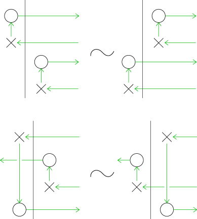
Figure 6. Two column commutations

A column commutation swaps two adjacent columns when either the two corresponding vertical strands project to disjoint vertical intervals, or one projected vertical interval is contained in the interior of the other. See Figure 6 for examples. A row commutation is similar but swaps adjacent rows.

Given a square in the grid diagram that is occupied by either an $X$ or an $O$, a stabilization splits the row and column of the square the symbol is in into two rows and two columns, replacing the $1\times 1$ marked square with a $2\times 2$ grid of which three squares are marked. For a given marker type (say, an $X$), there are four distinct ways to achieve this, corresponding to which square in the $2\times 2$ grid is unmarked. The rest of the diagram is left unchanged. See Figure 7 for examples. Destabilization is the process inverse to stabilization.

Figure 7. Stabilization; the diagram shows two possibilities out of the four

Proposition 1.10.

The isomorphism types of $\widetilde{\operatorname{GH}}$ and $\operatorname{GH}^{\mathord{-}}$ are invariant under a row or column commutation.

Proof.

Suppose that $\mathbb{G}_{1}$ and $\mathbb{G}_{2}$ are related by a column commutation. We can combine $\mathbb{G}_{1}$ and $\mathbb{G}_{2}$ into a single diagram, as in the right of Figure 8. Here, if we focus on the blue circle and erase the green circle, we obain (a diagram isotopic to) $\mathbb{G}_{1}$; similarly, erasing the blue circle, we obtain $\mathbb{G}_{2}$. Note that we position the blue and green curves so as to avoid triple intersections with horizontal circles. Label the intersection points between and blue and green circles by $a$ and $b$ as shown.

./images/grid-proof-invar-comm.pdf_tex

Figure 8. Combining two grid diagrams related by a column commutation into one diagram

The idea now is to use this combined diagram to define a chain homotopy equivalence $P_{1}\colon\operatorname{GC}^{\mathord{-}}(\mathbb{G}_{1})\to\operatorname{GC}^{\mathord{-}}(\mathbb{G}_{2})$, which counts empty pentagons. Instead of defining empty pentagons rigorously, we will just refer to Figure 8, and say that for $\operatorname{\mathbf{x}}\in\mathcal{S}(\mathbb{G}_{1})$ and $\operatorname{\mathbf{y}}\in\mathcal{S}(\mathbb{G}_{2})$, an element of $\operatorname{Pent}^{\mathord{\circ}}(\operatorname{\mathbf{x}},\operatorname{\mathbf{y}})$ is an embedded pentagon whose sides lie on the curves in the combined diagram, with vertices on $\operatorname{\mathbf{x}}$, $\operatorname{\mathbf{y}}$, and the distinguished point $a$, and leave the details to the reader. (Note that pentagons can exist to the left or the right of the column in question.) Then $P_{1}$ is defined by

$$P_{1}(\operatorname{\mathbf{x}})=\sum_{\operatorname{\mathbf{y}}\in\mathcal{S}(\mathbb{G}_{2})}\sum_{\begin{subarray}{c}p\in\operatorname{Pent}^{\mathord{\circ}}(\operatorname{\mathbf{x}},\operatorname{\mathbf{y}})\\ p\cap\mathbb{X}=\emptyset\end{subarray}}U_{1}^{O_{1}(p)}\dotsm U_{n}^{O_{n}(p)}\operatorname{\mathbf{y}}.$$

First, we need to show that $P_{1}$ is a chain map, i.e.,

$$\partial^{\mathord{-}}_{\operatorname{GC}^{\mathord{-}}(\mathbb{G}_{2})}\circ P_{1}+P_{1}\circ\partial^{\mathord{-}}_{\operatorname{GC}^{\mathord{-}}(\mathbb{G}_{1})}=0.$$

(Recall that we are in characteristic $2$.) The proof is similar to the proof that $\partial^{\mathord{-}}\circ\partial^{\mathord{-}}=0$, but we juxtapose a pentagon with a rectangle (in either order), instead of two rectangles.

Next, we need to show that $P_{1}$ has a homotopy inverse $P_{2}\colon\operatorname{GC}^{\mathord{-}}(\mathbb{G}_{2})\to\operatorname{GC}^{\mathord{-}}(\mathbb{G}_{1})$. The definition of $P_{2}$ is verbatim identical to that of $P_{1}$, but this time we count empty pentagons with a vertex on the distinguished point $b$ instead of $a$. The homotopies $H_{i}\colon\operatorname{GC}^{\mathord{-}}(\mathbb{G}_{i})\to\operatorname{GC}^{\mathord{-}}(\mathbb{G}_{i})$ are defined by counting empty hexagons that have both $a$ and $b$ as vertices. The claim is then that

$$P_{2}\circ P_{1}+\partial^{\mathord{-}}_{\operatorname{GC}^{\mathord{-}}(\mathbb{G}_{1})}\circ H_{1}+H_{1}\circ\partial^{\mathord{-}}_{\operatorname{GC}^{\mathord{-}}(\mathbb{G}_{1})} =\operatorname{Id}_{\operatorname{GC}^{\mathord{-}}(\mathbb{G}_{1})},$$

$$P_{1}\circ P_{2}+\partial^{\mathord{-}}_{\operatorname{GC}^{\mathord{-}}(\mathbb{G}_{2})}\circ H_{2}+H_{2}\circ\partial^{\mathord{-}}_{\operatorname{GC}^{\mathord{-}}(\mathbb{G}_{2})} =\operatorname{Id}_{\operatorname{GC}^{\mathord{-}}(\mathbb{G}_{2})}.$$

Indeed, most terms that appear on the left-hand side of these equations cancel out in pairs as in the proof that $\partial^{\mathord{-}}\circ\partial^{\mathord{-}}=0$, with the exception of domains that are topologically annuli, as in Figure 9, which cancel with the identity maps on the right-hand side.

./images/grid-proof-invar-comm-id.pdf_tex

Figure 9. Two annuli, one representing a term in $\partial^{\mathord{-}}_{\operatorname{GC}^{\mathord{-}}(\mathbb{G}_{1})}\circ H_{1}(\operatorname{\mathbf{x}})$ (left) and one representing a term in $P_{2}\circ P_{1}(\operatorname{\mathbf{x}}^{\prime})$ (right), that cancel with the identity. Here $\operatorname{\mathbf{x}}$ and $\operatorname{\mathbf{x}}^{\prime}$ (both in red) are two distinct generators in $\mathcal{S}(\mathbb{G}_{1})$. Note that there are other possibilities of such annular domains. Depending on $\operatorname{\mathbf{x}}$, there is always exactly one term that results in such an annular domain

The paragraphs above show that $(P_{1})_{*}\colon\operatorname{GH}^{\mathord{-}}(\mathbb{G}_{1})\to\operatorname{GH}^{\mathord{-}}(\mathbb{G}_{2})$ and $(P_{2})_{*}\colon$ $\operatorname{GH}^{\mathord{-}}(\mathbb{G}_{2})\to\operatorname{GH}^{\mathord{-}}(\mathbb{G}_{1})$ are inverses of each other, and are thus isomorphisms. The proof for row commutations is similar, and the proof for $\widetilde{\operatorname{GH}}$ is obtained by modifying the proof above to block all $O$ markers in all maps. ∎

The invariance of $\operatorname{GH}^{\mathord{-}}$ under (de)stabilization is quite a bit more tedious, and so we refer the reader to [31, Section 5.2] for full details. We simply give a brief outline here:

• First, we claim that the actions by the formal variables $U_{i}$ and $U_{j}$ on $\operatorname{GC}^{\mathord{-}}(\mathbb{G})$ are chain homotopic for all $i,j\in\{1,\dotsc,n\}$. The proof proceeds by defining a homotopy $\phi\colon\operatorname{GC}^{\mathord{-}}(\mathbb{G})\to\operatorname{GC}^{\mathord{-}}(\mathbb{G})$ that counts rectangles containing a single $X$ marker $X_{i}$ in it. One can show that

  $$\partial^{\mathord{-}}\circ\phi+\phi\circ\partial^{\mathord{-}}=U_{i}+U_{i+1},$$

  where the corresponding markers $O_{i}$ and $O_{i+1}$ are in the same row and same column as $X_{i}$ respectively; this proof is again similar to the proof that $\partial^{\mathord{-}}\circ\partial^{\mathord{-}}=0$.

• The upshot is that $\operatorname{GH}^{\mathord{-}}(\mathbb{G})$ can be thought of as an $\mathbb{F}[U]$-module, where $U$ acts by multiplication by any of the $U_{i}$’s.

• One then proceeds to prove that the isomorphism type of $\operatorname{GH}^{\mathord{-}}$ is invariant under (de)stabilization, by considering certain mapping cones. Combined with invariance under commutation, we see that the isomorphism type of $\operatorname{GH}^{\mathord{-}}(\mathbb{G})$ is a knot invariant, which we denote by $\operatorname{GH}^{\mathord{-}}(K)$.

• One may define the hat grid chain complex by setting one of the $U_{i}$’s to be zero, i.e.,

  $$\widehat{\operatorname{GC}}(\mathbb{G})=\operatorname{GC}^{\mathord{-}}(\mathbb{G})\otimes_{\mathbb{F}[U_{1},\dotsc,U_{n}]}\left(\faktor{\mathbb{F}[U_{1},\dotsc,U_{n}]}{U_{1}}\right).$$

  This has the effect of setting the action of $U$ to be zero, and so we get an $\mathbb{F}$-module $\widehat{\operatorname{GC}}(\mathbb{G})$. It is clear from the above that the isomorphism type of the $\mathbb{F}$-module $\widehat{\operatorname{GH}}(\mathbb{G})$ is also an invariant, which we denote by $\widehat{\operatorname{GH}}(K)$.

• Finally, we may place $\widetilde{\operatorname{GH}}(\mathbb{G})$ in this context also. Note that $\widetilde{\operatorname{GC}}(\mathbb{G})$ is obtained from $\widehat{\operatorname{GC}}(\mathbb{G})$ by also setting all the other $U_{i}$’s to zero. In other words, we have set $n-1$ “too many” $U_{i}$’s to be zero, and some homological algebra shows that

  $$\widetilde{\operatorname{GH}}(\mathbb{G})\cong\widehat{\operatorname{GH}}(\mathbb{G})\otimes_{\mathbb{F}}\mathbb{F}^{\otimes 2^{n-1}},$$

  and so the isomorphism type of $\widetilde{\operatorname{GH}}(\mathbb{G})$ is “almost” a knot invariant and can be denoted $\widetilde{\operatorname{GH}}(K,n)$.

We may summarize the invariance of grid homology here.

Theorem 1.11 (Manolescu, Ozsváth, and Sarkar [15, Theorem 1.1] and Manolescu, Ozsváth, Szabó, and Thurston [16, Theorem 1.2], cf. [31, Theorem 5.3.1]).

Let $\mathbb{G}$ be a grid diagram of $K\subset S^{3}$. The graded isomorphism types of $\operatorname{GH}^{\mathord{-}}(\mathbb{G})$ and $\widehat{\operatorname{GH}}(\mathbb{G})$ are invariants of the knot $K$. Thus, we may write $\operatorname{GH}^{\mathord{-}}(K)$ and $\widehat{\operatorname{GH}}(K)$ for these homologies.

Remark 1.12.

Instead of the homology, one may in fact state the invariance of the grid complex (and, later, of the Heegaard Floer complex) on the chain level: The graded chain homotopy type of the chain complex is an invariant. This is important, as many applications rely on invariants extracted from the chain complex.

In this lecture, we have chosen to exhibit in detail certain proofs while hiding others entirely. The point of showing the proof that $\partial^{\mathord{-}}_{\operatorname{GC}^{\mathord{-}}(\mathbb{G})}\circ\partial^{\mathord{-}}_{\operatorname{GC}^{\mathord{-}}(\mathbb{G})}=0$ in detail is that it is structurally the same as the proof that $\partial^{\mathord{-}}_{\operatorname{CF}^{\mathord{-}}(\mathcal{H})}\circ\partial^{\mathord{-}}_{\operatorname{CF}^{\mathord{-}}(\mathcal{H})}=0$ later, when we define the Heegaard Floer complex $\operatorname{CF}^{\mathord{-}}(\mathcal{H})$. There, the boundary homomorphism is defined by counting certain (pseudo)holomorphic bigons, and so the analysis becomes much more intricate; however, one will still consider a generator $\operatorname{\mathbf{z}}$ that appears in $\partial^{\mathord{-}}\circ\partial^{\mathord{-}}(\operatorname{\mathbf{x}})$, juxtapose two holomorphic bigons (analogous to rectangles here), and prove that there is an even number of ways that the resulting holomorphic curve can be decomposed into two holomorphic bigons that are counted.

Similarly, the proof that $\operatorname{GH}^{\mathord{-}}$ is invariant under commutation is structurally the same as the proof that $\operatorname{HF}^{\mathord{-}}$, the homology of $\operatorname{CF}^{\mathord{-}}$, is invariant under handleslides. There, one also combines multiple Heegaard diagrams (analogous to grid digrams) into a single diagram, define chain maps by counting holomorphic triangles (analogous to pentagons here), and define chain homotopies by counting holomorphic quadrilaterials (analogous to hexagons here).

Limited by time, we will not be able to delve into the details of these proofs in later lectures. However, it is my hope that the analogies above will provide some insight into them.

1.3. Maslov and Alexander gradings

Next, we move on to the homological grading of grid homology, known as the Maslov grading. This will allow us to discuss the graded isomorphism types of $\operatorname{GH}^{\mathord{-}}(K)$. While the definitions of gradings on Heegaard Floer homology are somewhat different in nature, the hope is that this will help us gain some insight into those gradings also. We continue to follow [31].

Definition 1.13.

Let $A$ and $B$ be two finite sets in $\mathbb{R}^{2}$. We define the following quantities:

$$\mathcal{I}(A,B)=\#\{(a,b)\in A\times B\,|\,a=(a_{1},a_{2}),\,b=(b_{1},b_{2}),\,a_{1}<b_{1},\,a_{2}<b_{2}\},$$

$$\mathcal{J}(A,B)=\frac{1}{2}(\mathcal{I}(A,B)+\mathcal{I}(B,A)).$$

In other words, $\mathcal{I}(A,B)$ counts the number of pairs of points $(a,b)\in A\times B$ such that $a$ is strictly to the southwest of $b$—such a pair is known as a northeast–southwest pair—and $\mathcal{J}$ symmetrizes $\mathcal{I}$.

Given $\operatorname{\mathbf{x}}\in\mathcal{S}(\mathbb{G})$, the Maslov grading $M(\operatorname{\mathbf{x}})=M_{\mathbb{O}}(\operatorname{\mathbf{x}})$ of $\operatorname{\mathbf{x}}$ is defined by

$$M(\operatorname{\mathbf{x}})=M_{\mathbb{O}}(\operatorname{\mathbf{x}})=\mathcal{J}(\operatorname{\mathbf{x}},\operatorname{\mathbf{x}})-2\mathcal{J}(\operatorname{\mathbf{x}},\mathbb{O})+\mathcal{J}(\mathbb{O},\mathbb{O})+1.$$

Proposition 1.14.

If there is a rectangle $r$ from $\operatorname{\mathbf{x}}$ to $\operatorname{\mathbf{y}}$, then

$$M(\operatorname{\mathbf{x}})-M(\operatorname{\mathbf{y}})=1-2\#(r\cap\mathbb{O}).$$

Proof.

If there are no $O$’s inside the rectangle $r$, then $\mathcal{J}(\operatorname{\mathbf{x}},\mathbb{O})=\mathcal{J}(\operatorname{\mathbf{y}},\mathbb{O})$ and $\mathcal{J}(\operatorname{\mathbf{x}},\operatorname{\mathbf{x}})-\mathcal{J}(\operatorname{\mathbf{y}},\operatorname{\mathbf{y}})=1$, because $r$ “destroys” a northeast–southwest pair in $\operatorname{\mathbf{x}}\times\operatorname{\mathbf{x}}$ to create a northwest–southeast pair in $\operatorname{\mathbf{y}}$, and $\operatorname{\mathbf{x}}$ and $\operatorname{\mathbf{y}}$ coincide everywhere else.

If $r\cap\mathbb{O}\neq\emptyset$, then for each $O$ inside the rectangle $r$, both $\mathcal{I}(\operatorname{\mathbf{x}},\mathbb{O})$ and $\mathcal{I}(\mathbb{O},\operatorname{\mathbf{x}})$ are increased by $1$; thus, $\mathcal{J}(\operatorname{\mathbf{x}},\mathbb{O})-\mathcal{J}(\operatorname{\mathbf{y}},\mathbb{O})$ counts the number of $O$’s inside $r$. ∎

This implies that $M$ induces a homological $\mathbb{Z}$-grading on $\widetilde{\operatorname{GC}}(\mathbb{G})$, since $r\cap\mathbb{O}=\emptyset$ in all relevant rectangles $r$ in the boundary homomorphism $\operatorname{\widetilde{\partial}}$.

For $\operatorname{GC}^{-}(\mathbb{G})$, note that $\#(r\cap\mathbb{O})$ may be a positive integer $m$. This would mean that $U^{m}\operatorname{\mathbf{y}}$ appears as a term in $\partial^{\mathord{-}}(\operatorname{\mathbf{x}})$, where by $U^{m}$ we mean a product of $m$ distinct $U_{i}$’s. Since $M(\operatorname{\mathbf{x}})-M(\operatorname{\mathbf{y}})=1-2m$, if we set $M(U_{i})=-2$ for all $U_{i}$’s, then

$$M(U^{m}\operatorname{\mathbf{y}})=M(U^{m})+M(\operatorname{\mathbf{y}})=-2m+(M(\operatorname{\mathbf{x}})-1+2m)=M(\operatorname{\mathbf{x}})-1,$$

and we have a homological $\mathbb{Z}$-grading on $\operatorname{GC}^{\mathord{-}}(\mathbb{G})$.

Remark 1.15.

The reason that we have a homological $\mathbb{Z}$-grading on $\operatorname{GH}^{\mathord{-}}(K)$ is because, as we shall see, it is a version of knot Floer homology in the three-sphere, $\operatorname{HFK}^{\mathord{-}}(S^{3},K)$. For a general $3$-manifold $Y$, neither $\operatorname{HF}^{\mathord{-}}(Y)$ nor $\operatorname{HFK}^{\mathord{-}}(Y,K)$ is necessarily $\mathbb{Z}$-graded; in fact, one may get different $\mathbb{Z}/m$ gradings for different $\operatorname{Spin^{c}}$-structures on $Y$. These gradings are also not necessarily absolute, meaning that they may be well-defined only up to a constant shift. We will briefly discuss the $\operatorname{Spin^{c}}$-decomposition and gradings in the last lecture.

In fact, $\widetilde{\operatorname{GC}}(\mathbb{G})$ and $\operatorname{GC}^{\mathord{-}}(\mathbb{G})$ are equipped with an internal grading $A$ (meaning that the boundary homomorphism preserves $A$), known as the Alexander grading.

Definition 1.16.

Given $\operatorname{\mathbf{x}}\in\mathcal{S}(\mathbb{G})$, the Alexander grading $A(\operatorname{\mathbf{x}})$ of $\operatorname{\mathbf{x}}$ is defined by

$$A(\operatorname{\mathbf{x}})=\frac{1}{2}(M_{\mathbb{O}}(\operatorname{\mathbf{x}})-M_{\mathbb{X}}(\operatorname{\mathbf{x}}))-\frac{n-1}{2},$$

where $M_{\mathbb{X}}$ is defined in the same way as $M_{\mathbb{O}}$ but with $\mathbb{O}$ replaced by $\mathbb{X}$ in its definition.

The existence of $A$ is a feature of knot Floer invariants (e.g., $\operatorname{CFK}^{\mathord{-}}$) and can be understood in terms of a “relative” $\operatorname{Spin^{c}}$-decomposition. We will not discuss it further until the final lecture, but will point out that $A$ plays an important role in many applications; for example, see Remark 1.18.

1.4. Graded isomorphism types

From now until the final lecture, we will focus only on the Maslov grading and ignore the Alexander grading.

Let us now look at the possible graded isomorphism types that the various flavors of grid homology can have, starting with $\widetilde{\operatorname{GH}}(K,n)$ and $\widehat{\operatorname{GH}}(K)$. Since they are finitely generated graded $\mathbb{F}$-modules (that is to say, $\mathbb{F}$–vector spaces), they must have graded isomorphism types

$$\bigoplus_{m\in\mathbb{Z}}\mathbb{F}_{(m)}^{\oplus a_{m}}\quad\text{with}\quad\sum_{m}a_{m}<\infty,$$

where $\mathbb{F}_{(m)}$ denotes a summand in Maslov grading $m$.

As for $\operatorname{GH}^{-}$, it is an $\mathbb{F}[U]$-module. Since $\mathbb{F}[U]$ is a principal ideal domain, the Fundamental Theorem for Finitely Generated Modules over a Principal Ideal Domain implies that $\operatorname{GH}^{-}(K)$ is a direct sum of cyclic modules, i.e., it must have ungraded isomorphism type

$$\operatorname{GH}^{-}(K)\cong\mathbb{F}[U]^{\oplus a}\oplus\left(\faktor{\mathbb{F}[U]}{(f_{1}(U))}\right)\oplus\dotsb\oplus\left(\faktor{\mathbb{F}[U]}{(f_{k}(U))}\right),$$

where the $f_{i}$’s are polynomials. Moreover, since $U$ strictly decreases grading, the $f_{i}$’s must actually be monomials! Hence, we have

$$\operatorname{GH}^{-}(K)\cong\mathbb{F}[U]^{\oplus a}\oplus\left(\faktor{\mathbb{F}[U]}{U^{b_{1}}}\right)\oplus\dotsb\oplus\left(\faktor{\mathbb{F}[U]}{U^{b_{k}}}\right).$$

Remark 1.17.

This last assertion is no longer true if the grading is a $\mathbb{Z}/m$-grading instead of a $\mathbb{Z}$-grading, because $U^{m/2}\operatorname{\mathbf{x}}$ can now have the same grading as $\operatorname{\mathbf{x}}$. This may occur for the Heegaard Floer homology of a general $3$-manifold.

One can, of course, write a graded version of this statement as well, which is left to the reader.

It turns out that, because $\operatorname{GH}^{\mathord{-}}(K)$ is a version of $\operatorname{HFK}^{\mathord{-}}(S^{3},K)$, i.e., the ambient $3$-manifold is $S^{3}$, there is only one $\mathbb{F}[U]$-summand, meaning that $a=1$.

Remark 1.18.

The invariant $\tau(K)$ is defined as $-A$, where $A$ is the (top) Alexander grading of the generator of the $\mathbb{F}[U]$-summand of $\operatorname{HFK}^{\mathord{-}}(K)$. $\tau$ provides a very useful concordance homomorphism.

One feature that is often overlooked is that the graded isomorphism type of $\widehat{\operatorname{GH}}(K)$ is completely determined by that of $\operatorname{GH}^{\mathord{-}}(K)$. Indeed, note that

$$\widehat{\operatorname{GC}}(\mathbb{G})\cong\operatorname{GC}^{-}(\mathbb{G})\otimes_{\mathbb{F}[U]}\left(\faktor{\mathbb{F}[U]}{U}\right).$$

Thus, the Universal Coefficient Theorem implies that

$$\widehat{\operatorname{GH}}(K)\cong\operatorname{GH}^{-}(K)\otimes_{\mathbb{F}[U]}\left(\faktor{\mathbb{F}[U]}{U}\right)\oplus\operatorname{Tor}_{1}^{\mathbb{F}[U]}\left(\operatorname{GH}^{-}(K),\faktor{\mathbb{F}[U]}{U}\right).$$

Example 1.19.

With some work, one can work out the minus grid homology of the left-handed trefoil to be

$$\operatorname{GH}^{-}(\overline{T}_{2,3})\cong(\mathbb{F}[U])_{(2)}\oplus\left(\faktor{\mathbb{F}[U]}{U}\right)_{(1)},$$

and so we can also read off the hat grid homology to be

$$\widehat{\operatorname{GH}}(\overline{T}_{2,3}) \cong\left(\faktor{\mathbb{F}[U]}{U}\right)_{(2)}\oplus\left(\faktor{\mathbb{F}[U]}{U}\right)_{(1)}\oplus\left(\faktor{\mathbb{F}[U]}{U}\right)_{(0)}$$

$$\cong\mathbb{F}_{(2)}\oplus\mathbb{F}_{(1)}\oplus\mathbb{F}_{(0)}.$$

Exercise 1.20.

Compute $\operatorname{Tor}_{1}$ here. Bonus: Compute it with gradings.

1.5. Other flavors

Finally, we mention some more flavors of grid homology. First, we have the infinity and plus flavors.

Definition 1.21.

The infinity and plus grid chain complexes are defined respectively by

$$\operatorname{GC}^{\infty}(\mathbb{G}) =\operatorname{GC}^{-}(\mathbb{G})\otimes_{\mathbb{F}[U]}\mathbb{F}[U,U^{-1}],$$

$$\operatorname{GC}^{+}(\mathbb{G}) =\operatorname{GC}^{\infty}(\mathbb{G})\otimes_{\mathbb{F}[U]}\left(\faktor{\mathbb{F}[U,U^{-1}]}{U}\right),$$

both thought of as (bi)graded chain complexes of $\mathbb{F}[U]$-modules.

One can recover $\operatorname{GC}^{\mathord{-}}(\mathbb{G})$ from $\operatorname{GC}^{\infty}(\mathbb{G})$ as a subcomplex, and $\operatorname{GC}^{\mathord{+}}(\mathbb{G})$ from $\operatorname{GC}^{\infty}(\mathbb{G})$ as a quotient complex, and so these three flavors contain roughly the same amount of information.

Exercise 1.22.

Work out some obvious mapping cones among the minus, plus, infinity, and hat flavors of grid chain complexes.

All of these flavors are considered in the literature, as it is often easier to formulate a certain statement in one flavor versus another. They also all appear in general Heegaard Floer homology, as $\operatorname{CF}^{\mathord{-}}(\mathcal{H})$, $\operatorname{CF}^{\mathord{+}}(\mathcal{H})$, $\operatorname{CF}^{\infty}(\mathcal{H})$, and $\widehat{\operatorname{CF}}(\mathcal{H})$. In each of these cases, the graded isomorphism type of the homology (or in fact, the graded chain homotopy type of the chain complex) is an invariant.

Remark 1.23.

Again by the Universal Coefficient Theorem, one can compute

$$\operatorname{GH}^{\infty}(K)\cong\mathbb{F}[U,U^{-1}],$$

and so the infinity homology is not very interesting. However, the infinity chain complex $\operatorname{GC}^{\infty}(K)$ enjoys a rich structure, and many invariants, such as $\epsilon(K)$ [7] and $\Upsilon(K)$ [32], can be extracted from it.

There are more flavors that are worth noting:

• If we allow rectangles to contain $X$’s but do not record them, the Alexander grading is no longer an internal grading; instead, it can be lowered by the boundary homomorphism, meaning that it becomes only a filtration. (The Maslov grading remains a homological grading.) The filtered, graded homotopy type of this filtered chain complex, denoted $\mathcal{GC}^{-}(\mathbb{G})$, is a knot invariant. To recover $\operatorname{GC}^{\mathord{-}}(K)$, one takes the associated graded object of $\mathcal{GC}^{-}(K)$, which exactly blocks all rectangles that contain $X$’s. The object in general Heegaard Floer theory analogous to $\mathcal{GC}^{-}(K)$ is $\operatorname{CFK}^{\mathord{-}}(Y,K)$, which is a filtered, graded chain complex, and $\operatorname{HFK}^{\mathord{-}}(Y,K)$, which is analogous to $\operatorname{GH}^{\mathord{-}}(K)$, is the homology of the associated graded object of $\operatorname{CFK}^{\mathord{-}}(Y,K)$.

• An approach alternative to filtered complexes is to introduce formal variables $V_{i}$ for $X_{i}$, and define

  $$\partial^{\mathord{-}}_{\mathbb{O}\mathbb{X}}(\operatorname{\mathbf{x}})=\sum_{\operatorname{\mathbf{y}}\in\mathcal{S}(\mathbb{G})}\sum_{r\in\operatorname{Rect}^{\mathord{\circ}}(\operatorname{\mathbf{x}},\operatorname{\mathbf{y}})}U_{1}^{O_{1}(r)}\dotsm U_{n}^{O_{n}(r)}V_{1}^{X_{1}(r)}\dotsm V_{n}^{X_{n}(r)}\operatorname{\mathbf{y}},$$

  This is the approach taken in [44, 43] and some other recent work. However, one must grapple with the fact that $\partial^{\mathord{-}}_{\mathbb{O}\mathbb{X}}\circ\partial^{\mathord{-}}_{\mathbb{O}\mathbb{X}}\equiv c\neq 0$, where $c\in\mathcal{R}$ is the curvature of a curved chain complex.

• We can also set $U_{1}=\dots=U_{n}=V_{1}=\dots=V_{n}$ and consider a chain complex with

  $$\partial^{{}^{\prime}}(\operatorname{\mathbf{x}})=\sum_{\operatorname{\mathbf{y}}\in\mathcal{S}(\mathbb{G})}\sum_{r\in\operatorname{Rect}^{\mathord{\circ}}(\operatorname{\mathbf{x}},\operatorname{\mathbf{y}})}U^{O(r)+X(r)}\operatorname{\mathbf{y}}.$$

  Since $O$’s and $X$’s are treated equally in the boundary homomorphism, we lose the information of the orientation of the knot. This is called unoriented grid homology [33].

2. “Naive” Heegaard Floer homology

2.1. Definition

Having caught a glimpse of some of the features of Heegaard Floer homology as exhibited in grid homology, the rest of this lecture will be devoted to discussing a “naive” definition of Heegaard Floer homology, where the boundary homomorphism counts domains on a Heegaard diagram, just as the grid boundary homomorphism counts rectangles on a grid diagram. For someone unacquainted with Heegaard Floer homology attending a research talk on the subject, this may seem like what is going on when the speaker shades certain domains on a Heegaard diagram. However, this is not the actual definition of Heegaard Floer homology, as it may not even produce a legitimate chain complex. And yet, I think there is some merit in investigating this “naive” definition.

This exercise serves several purposes. First, not yet burdened with the analysis involved in Morse or Floer theory, we can transfer some of the intuition we gained from grid homology to help us make sense of some definitions. Second, by looking at some of the simplest examples, for which the “naive” definition seems to make sense, we can get a taste of some of the issues that must be addressed in the actual theory. Third, by looking at an example where $\partial^{2}\not\equiv 0$, we will get to see why the “naive” definition cannot make sense.

We assume familiarity with Heegaard diagrams of $3$-manifolds. In Heegaard Floer homology, we consider pointed $3$-manifolds $(Y,z)$, where $z\in Y$. Correspondingly, we consider pointed Heegaard diagrams $\mathcal{H}=(\Sigma,\bm{\alpha},\bm{\beta},z)$. As usual, if $\Sigma$ has genus $g$, then $\bm{\alpha}$ is a set of $g$ mutually disjoint circles $\{\alpha_{1},\dotsc,\alpha_{g}\}$ on $\Sigma$, and $\bm{\beta}$ is a set of $g$ mutually disjoint circles $\{\beta_{1},\dotsc,\beta_{g}\}$. We often abuse notation and use $\bm{\alpha}$ to denote $\alpha_{1}\cup\dotsb\cup\alpha_{g}$ and $\bm{\beta}$ to denote $\beta_{1}\cup\dotsb\cup\beta_{g}$. We assume that $z$ lies on $\Sigma$ away from all $\alpha$- and $\beta$-curves.

Example 2.1.

Figure 10 shows two pointed Heegaard diagrams of $(S^{3},z)$, while Figure 11 shows two diagrams of $(S^{1}\times S^{2},z)$. As is customary, $\alpha$-curves are colored red, while $\beta$-curves are colored blue.

./images/HD-S3.pdf_tex

(a) $\mathcal{H}_{1}$

./images/HD-S3-admissible.pdf_tex

(b) $\mathcal{H}_{2}$

Figure 10. Two Heegaard diagrams of $(S^{3},z)$

./images/HD-S1xS2-a.pdf_tex

(a) $\mathcal{H}_{3}$

./images/HD-S1xS2-b.pdf_tex

(b) $\mathcal{H}_{4}$

Figure 11. Two Heegaard diagrams of $(S^{1}\times S^{2},z)$

Inspired by the grid chain complexes, here is a “naive” definition of the Heegaard Floer chain complex associated to a pointed Heegaard diagram.

Definition 2.2.

Given a pointed Heegaard diagram $\mathcal{H}=(\Sigma,\bm{\alpha},\bm{\beta},z)$, we define the generating set

$$\mathcal{S}(\mathcal{H})=\{\text{matchings between $\bm{\alpha}$ and $\bm{\beta}$ in }\mathcal{H}\},$$

where a matching is a one-to-one correspondence between the $\alpha$- and $\beta$-circles.

We define the hat and minus “naive” Heegaard Floer chain complexes respectively as the $\mathbb{F}$-module and the $\mathbb{F}[U]$-module

$$\widehat{\operatorname{CF}}(\mathcal{H})=\mathbb{F}\langle\mathcal{S}(\mathcal{H})\rangle,\qquad\operatorname{CF}^{\mathord{-}}(\mathcal{H})=\mathbb{F}[U]\langle\mathcal{S}(\mathcal{H})\rangle,$$

with boundary homomorphisms $\widehat{\partial}\colon\widehat{\operatorname{CF}}(\mathcal{H})\to\widehat{\operatorname{CF}}(\mathcal{H})$ and $\partial^{\mathord{-}}\colon\operatorname{CF}^{\mathord{-}}(\mathcal{H})\to\operatorname{CF}^{\mathord{-}}(\mathcal{H})$ given by

$$\widehat{\partial}(\operatorname{\mathbf{x}})=\sum_{\operatorname{\mathbf{y}}\in\mathcal{S}(\mathcal{H})}\sum_{\begin{subarray}{c}p\in\pi_{2}(\operatorname{\mathbf{x}},\operatorname{\mathbf{y}})\\ p\cap\{z\}=\emptyset\end{subarray}}\operatorname{\mathbf{y}},\qquad\partial^{\mathord{-}}(\operatorname{\mathbf{x}})=\sum_{\operatorname{\mathbf{y}}\in\mathcal{S}(\mathcal{H})}\sum_{p\in\pi_{2}(\operatorname{\mathbf{x}},\operatorname{\mathbf{y}})}U^{n_{z}(p)}\operatorname{\mathbf{y}},$$

where $n_{z}(p)$ is the multiplicity of $z$ in $p$, and $\pi_{2}(\operatorname{\mathbf{x}},\operatorname{\mathbf{y}})$ denotes the space of domains from $\operatorname{\mathbf{x}}$ to $\operatorname{\mathbf{y}}$. Here, a region is a connected component of $\Sigma\setminus(\bm{\alpha}\cup\bm{\beta})$, and a domain $p$ from $\operatorname{\mathbf{x}}$ to $\operatorname{\mathbf{y}}$ is a $2$-chain on $\Sigma$ that is a linear combination of regions with non-negative coefficients, such that

$$\partial((\partial p)\cap\bm{\alpha})=\operatorname{\mathbf{y}}-\operatorname{\mathbf{x}}$$

in the induced orientation on $\partial p$.

Something seems immediately suspicious in this definition. Indeed, if we concatenate a domain from $\operatorname{\mathbf{x}}$ to $\operatorname{\mathbf{y}}$ and a domain from $\operatorname{\mathbf{y}}$ to $\operatorname{\mathbf{z}}$, we will get a domain from $\operatorname{\mathbf{x}}$ to $\operatorname{\mathbf{z}}$; but clearly we do not want a scenario where $\operatorname{\mathbf{y}}$ appears as a term in $\partial(\operatorname{\mathbf{x}})$, and $\operatorname{\mathbf{z}}$ appears as a term in both $\partial(\operatorname{\mathbf{y}})$ and $\partial(\operatorname{\mathbf{x}})$. In grid homology, concatenating two rectangles always results in a domain that is not a rectangle; here, we need to instead rely on a Maslov index on elements of $\pi_{2}(\operatorname{\mathbf{x}},\operatorname{\mathbf{y}})$. We will not go into details here, except that such an index exists and can be computed [11, Corollary 4.10], and gives rise to the homological Maslov grading on our chain complex. The idea, then, is that we will only count domains that are of index $1$; concatenating two such domains will give a domain of index $2$, which is not counted. Applying this idea back to the grid chain complex, this would eliminate

• domains that have reflex angles in them; and

• domains that contain points in $\operatorname{\mathbf{x}}$ or $\operatorname{\mathbf{y}}$ in them.

This is why only empty rectangles are counted in grid homology. In any case, this represents the first modification we would like to make.

When $g(\Sigma)=1$, the condition that a domain must be of Maslov index $1$ will imply that it must in fact be an immersed bigon with non-reflex angles at its corners. (A bigon is a disk with two corners.)

Example 2.3.

We can compute the chain complexes associated to the two diagrams of $(S^{3},z)$ in Example 2.1. For $\mathcal{H}_{1}$, let $x$ be the unique intersection point of the $\alpha$ and $\beta$ curves. Since there are no domains, it follows that

$$\widehat{\operatorname{CF}}(\mathcal{H}_{1}) \cong\mathbb{F}\langle x\rangle, \operatorname{CF}^{-}(\mathcal{H}_{1}) \cong\mathbb{F}[U]\langle x\rangle, \widehat{\partial} \equiv 0\equiv\partial^{-},$$

$$\widehat{\operatorname{HF}}(\mathcal{H}_{1}) \cong\mathbb{F}, \operatorname{HF}^{\mathord{-}}(\mathcal{H}_{1}) \cong\mathbb{F}[U].$$

For $\mathcal{H}_{2}$, labeling the intersection points by $a$, $b$, and $c$ as in Figure 10(b), there are two domains, one from $a$ to $b$ containing $z$, and one from $c$ to $b$ not containing $z$. Thus,

$$\widehat{\operatorname{CF}}(\mathcal{H}_{2})\cong\mathbb{F}\langle a,b,c\rangle, \operatorname{CF}^{-}(\mathcal{H}_{2})\cong\mathbb{F}[U]\langle a,b,c\rangle,$$

$$\widehat{\partial}(a)=\widehat{\partial}(b)=0,\quad\widehat{\partial}(c)=b,\quad \partial^{\mathord{-}}(a)=Ub,\quad\partial^{\mathord{-}}(b)=0,\quad\partial^{\mathord{-}}(c)=b,$$

$$\widehat{\operatorname{HF}}(\mathcal{H}_{2})\cong\mathbb{F}\langle a,b\rangle/(b)\cong\mathbb{F}, \operatorname{HF}^{\mathord{-}}(\mathcal{H}_{2})\cong\mathbb{F}[U]\langle a+Uc,b\rangle/(b)\cong\mathbb{F}[U].$$

2.2. Admissibility

So far, we have not run into any major problems. Let us look an example that seems more mysterious:

Example 2.4.

We now look at the two diagrams of $(S^{1}\times S^{2},z)$ in Example 2.1. One can compute that

$$\widehat{\operatorname{HF}}(\mathcal{H}_{3})\cong\mathbb{F}\oplus\mathbb{F},\qquad\widehat{\operatorname{HF}}(\mathcal{H}_{4})\cong 0,$$

and

$$\operatorname{HF}^{-}(\mathcal{H}_{3})\cong\mathbb{F}[U]\oplus\mathbb{F}[U],\qquad\operatorname{HF}^{-}(\mathcal{H}_{4})\cong\faktor{\mathbb{F}[U]}{(1+U)}.$$

This seems to suggest that $\widehat{\operatorname{HF}}$ and $\operatorname{HF}^{\mathord{-}}$ are not invariants of $3$-manifolds! One may naturally suspect that the culprit is the “naive” definition, but in fact, it is not—we are indeed computing the correct chain complexes here.

So what gives? It turns out that this has to do with a requirement on the Heegaard diagrams called admissibility, a condition that guarantees the diagram to be suitable for computation. In other words, we cannot simply choose any Heegaard diagram and expect it to give us the correct answer. This is closely related to the $\operatorname{Spin^{c}}$-decomposition of Heegaard Floer homology, and we will briefly touch upon this issue again in the last lecture.

2.3. $\partial^{2}\equiv 0$

There is, in fact, a more serious problem that has been lurking in our “naive” approach to the Heegaard Floer complex: We have not proved $\partial^{2}\equiv 0$ for either the hat or the minus flavor; in other words, we do not know that we have defined chain complexes.

This turns out to be a real problem. See Figure 12; the shaded domain has three decompositions into domains, each of which has the correct index. This means that $\operatorname{\mathbf{z}}$ (in green) appears as a term in $\widehat{\partial}\circ\widehat{\partial}(\operatorname{\mathbf{x}})$ that is not canceled by any other term.

./images/composite-domain.pdf_tex

Figure 12. A composite domain that has three decompositions into domains that are counted in the differential

This illustrates a key point, upon understanding which, we graduate from the “naive” approach: The Heegaard Floer chain complex is not supposed to be defined by counting polygons on a Heegaard diagram. Instead, it is defined by counting (pseudo)holomorphic curves on a space associated to the Heegaard diagram, distinct from the Heegaard diagram itself unless $g(\Sigma)=1$. One can think of the domains we have been counting as “shadows” of such holomorphic curves; given a domain of the right index, there may be $0$, $1$, or any number of holomorphic curves with that shadow. It is the count of holomorphic curves, rather than the count of domains, that satisfies $\partial^{2}\equiv 0$.

3. Lagrangian Floer homology

3.1. Setup

So now we understand that the boundary homomorphism in the Heegaard Floer chain complex counts certain holomorphic curves in some yet mysterious space. One of the questions most often asked is “why”: What is the motivation behind the Heegaard Floer complex? In this lecture, we attempt to address this by providing an introduction to Lagrangian Floer homology; in short, Heegaard Floer homology can be defined via Lagrangian Floer homology, which in turn can be understood as a kind of infinite-dimensional Morse homology.

Lagrangian intersection Floer homology (or simply Lagrangian Floer homology) is an invariant of $\left(M,\omega,L_{0},L_{1}\right)$, where $(M,\omega)$ is a symplectic manifold, and $L_{0}$, $L_{1}$ are two transversely intersecting Lagrangian submanifolds of $(M,\omega)$. The following is a quick survey that mostly follows the exposition in [36]. We will make whichever assumptions we need to simplify the exposition, regardless of whether they hold in Heegaard Floer theory. First, we will assume that $\pi_{2}(M)=0$—or less restrictively,

(1) $$\int_{S^{2}}f^{*}\omega=0$$

for all $\left[f\right]\in\pi_{2}(M)$—and $\pi_{1}(L_{i})=0$ for each $i=0,1$.

The idea is to perform “Morse homology” on an infinite-dimensional manifold associated to $(M,\omega,L_{0},L_{1})$ defined as follows. Consider first

$$\mathcal{P}=\mathcal{P}(L_{0},L_{1})=\{\gamma\colon[0,1]\to M\,|\,\gamma\text{ is smooth},\,\gamma(0)\in L_{0},\,\gamma(1)\in L_{1}\},$$

the set of smooth paths from $L_{0}$ to $L_{1}$, with the $\mathcal{C}^{\infty}$ topology. Note that $\mathcal{P}$ is not necessarily connected. Choose an element $\widehat{\gamma}\in\mathcal{P}$ (and by doing so, a connected component of $\mathcal{P}$), and consider the universal cover $\widetilde{\mathcal{P}}$ based at $\widehat{\gamma}$.

This means that we get a set of paths of paths:

$$\begin{split}\widetilde{\mathcal{P}}=\widetilde{\mathcal{P}}(L_{0},L_{1};\widehat{\gamma})&=\{(\gamma,w)\,|\,\gamma\in\mathcal{P},w\text{ is a path from }\widehat{\gamma}\text{ to }\gamma,\textit{ i.e.}\\ &\qquad w\colon[0,1]\times[0,1]\to M\text{ with }w(\cdot,r)\in\mathcal{P}\text{ for all }r\in[0,1],\\ &\qquad w(s,0)=\widehat{\gamma}(s),\,w(s,1)=\gamma(s)\text{ for all }s\in[0,1]\}/\sim,\end{split}$$

where $(\gamma,w)\sim(\gamma,w^{\prime})$ if $w,w^{\prime}$ are homotopic relative to $(\widehat{\gamma},\gamma)$.

./images/L0intL1-homotopy.pdf_tex

Figure 13. A path $w$ from $\widehat{\gamma}$ to $\gamma$, where each value of $r$ gives a path $w(\cdot,r)$ from $L_{0}$ to $L_{1}$

It is on this space that we will apply “Morse homology”.

3.2. Morse homology: An interlude

We briefly recall here the construction of Morse homology. Let $M$ be a closed, smooth manifold. Recall that a smooth function $f\colon M\to\mathbb{R}$ is Morse if at each of its critical points (where in local coordinates all first derivatives $\partial f/\partial x_{i}$ vanish), the Hessian matrix $H=(\partial^{2}f/\partial x_{i}\partial x_{j})$ is not degenerate (i.e., has non-zero determinant). By the Morse Lemma, all such critical points must be isolated. The Morse index $\operatorname{Ind}(x)$ of a non-degenerate critical point $x$ is the dimension of the largest subspace of the tangent space that is negative definite. Classical Morse theory says that Morse functions are generic, and that, given a Morse function $f$, $M$ is homotopy equivalent to a CW complex with an $n$-cell for each critical point of $f$ of index $n$.

In fact, one can even reconstruct a CW chain complex of $M$ using $f$ and auxiliary data. Since the critical points of $f$ correspond to cells in a CW complex, let $\operatorname{CM}(M;f)$ be the $\mathbb{F}$-module generated by the critical points of $f$. To define a boundary homomorphism the idea is to count the number of negative gradient flow lines from a critical point of index $n$ to one of index $n-1$. The notion of the gradient requires the choice of a Riemannian metric $g$ on $M$, meaning that we will have a chain complex $\operatorname{CM}(M;f,g)=\operatorname{CM}(M;f)$, with boundary homomorphism $\partial\colon\operatorname{CM}(M;f,g)\to\operatorname{CM}(M;f,g)$. Concretely, we consider the moduli space $\mathcal{M}_{g}(x,y)$ of curves $u\colon\mathbb{R}\to M$ satisfying

• $\displaystyle\frac{du}{dt}=-\operatorname{grad}f$;

• $\lim_{t\to-\infty}u(t)=x$; and

• $\lim_{t\to\infty}u(t)=y$.

To ensure that $\mathcal{M}_{g}(x,y)$ is a manifold of dimension $\operatorname{Ind}(x)-\operatorname{Ind}(y)$, the pair $(f,g)$ needs to satisfy the Morse–Smale condition, which is luckily also generic. (The desired property that $\mathcal{M}_{g}(x,y)$ is be a manifold of the right dimension, is known as transversality.) There is a natural action of $\mathbb{R}$ on $\mathcal{M}_{g}(x,y)$ by shifting $t\in\mathbb{R}$; to consider flow lines rather than flows, one takes the quotient $\mathcal{M}_{g}(x,y)/\mathbb{R}$, which has dimension $\operatorname{Ind}(x)-\operatorname{Ind}(y)-1$. The manifold $\mathcal{M}_{g}(x,y)/\mathbb{R}$ can be compactified to a compact manifold $\widehat{\mathcal{M}}_{g}(x,y)$ with boundary by including the limits of sequences of elements, which are broken gradient flow lines. (The desired property that $\mathcal{M}_{g}(x,y)$ can be compactified to a compact manifold with boundary is known as compactness.) When the index difference between $x$ and $y$ is $1$, the moduli space $\widehat{\mathcal{M}}_{g}(x,y)$ is a compact manifold of dimension $0$. Thus, one can define the matrix element $\langle\partial x,y\rangle$ as follows: If $\operatorname{Ind}(x)-\operatorname{Ind}(y)=1$, it is the number of elements in $\widehat{\mathcal{M}}_{g}(x,y)$ modulo $2$; otherwise, it is $0$.

To show that $\partial^{2}\equiv 0$, we consider $\widehat{\mathcal{M}}_{g}(x,z)$ where $\operatorname{Ind}(x)-\operatorname{Ind}(z)=2$. This is a compact $1$-dimensional manifold with boundary, and so there is an even number of boundary points; since these correspond to broken flow lines from $x$ to $z$ that appear in $\partial\circ\partial(x)$, this means that all terms cancel in pairs.

The main result is then that the Morse homology

$$\operatorname{HM}(M;f,g)=H_{*}(\operatorname{CM}(M;f,g),\partial)$$

is isomorphic to the CW or singular homology $H_{*}(M;\mathbb{Z}/2)$ of $M$. One could deduce from this that $\operatorname{HM}(M;f,g)$ is invariant under a different choice of $f$ or $g$. Absent the isomorphism with singular homology, one would need to define chain homotopy equivalences between $\operatorname{CM}(M;f,g)$ and $\operatorname{CM}(M;f^{\prime},g^{\prime})$. This is important, since in the context of Floer homology, there is often no classical invariant to rely on, and this is the only way to prove invariance.

3.3. The differential

Turning back to Lagrangian Floer homology, we would like to follow the steps above in this setting. The role of the manifold $M$ will be played by the space $\widetilde{\mathcal{P}}$; what we need now is a “Morse function”.

Definition 3.1.

The action functional $\mathcal{A}\colon\widetilde{\mathcal{P}}\to\mathbb{R}$ is defined by

$$\mathcal{A}\left([\gamma,w]\right)=\int_{[0,1]^{2}}w^{*}\omega.$$

(Here and below, we abbreviate $[(\gamma,w)]$ to $[\gamma,w]$.) We need to check that it does not depend on the choice of $w$, i.e., that we have

(2) $$(\gamma,w)\sim(\gamma,w^{\prime})\implies\mathcal{A}([\gamma,w])=\mathcal{A}([\gamma,w^{\prime}]).$$

This follows from Equation (1).

Exercise 3.2.

Verify Equation (2).

In local coordinates, we have

$$w^{*}\omega\left(\frac{\partial}{\partial s},\frac{\partial}{\partial r}\right)=\omega\left(\frac{\partial w}{\partial s},\frac{\partial w}{\partial r}\right),$$

and so

$$\mathcal{A}\left([\gamma,w]\right)=\int_{0}^{1}\int_{0}^{1}\omega\left(\frac{\partial w}{\partial s},\frac{\partial w}{\partial r}\right)\,dr\,ds.$$

Now, we want to run “Morse homology” on $(\widetilde{\mathcal{P}},\mathcal{A})$, which is structurally similar to the finite-dimensional case but has a lot of technicalities that come with infinite-dimensional spaces.

Let us compute $\operatorname{grad}\mathcal{A}$. We need a Riemannian metric on $\widetilde{\mathcal{P}}$, which we will get by integrating a Riemannian metric on $M$. This is possible because a tangent vector $\xi\in T_{[\gamma,w]}\widetilde{\mathcal{P}}$ can be regarded, roughly, as an infinitesimal change to $\gamma(s)$ for every $s\in[0,1]$; in other words, it can be viewed as a collection of tangent vectors $\xi(s)\in T_{\gamma(s)}M.$

We will find a natural metric on $M$ using $\omega$ and a further choice. Recall that the following structures are related.

Here, a choice of any two of these structures that are compatible determines the third one. This is related to the structure groups of these structures, which are subgroups of $GL_{2n}(\mathbb{R})$.

The intersection of any two of these is $U(n)$. The notion of compatibility mentioned above is specified in the following definition.

Definition 3.3.

An almost complex structure $J$ is compatible with $\omega$ if

(3) $$\omega(Jv,J{v^{\prime}}) =\omega(v,v^{\prime}) \text{for all }v,v^{\prime}\in T_{p}M,$$

(4) $$\omega(v,Jv) >0 \text{for all }v\neq 0\in T_{p}M.$$

It can be shown that compatible almost complex structures on symplectic manifolds are abundant.

Given $\omega$ and a compatible $J$, we can now define the metric $g_{J}$ by the formula

(5) $$g_{J}(v,v^{\prime})=\omega(v,Jv^{\prime}).$$

Exercise 3.4.

Check that $g_{J}$ is a Riemannian structure.

With a metric $g_{J}$ on $M$, we can define a metric on $\widetilde{\mathcal{P}}$ as follows: Given $\xi_{1},\xi_{2}\in T_{[\gamma,w]}\widetilde{\mathcal{P}}$, we can define

$$\langle\xi_{1},\xi_{2}\rangle=\int_{0}^{1}g_{J}(\xi_{1}(s),\xi_{2}(s))\,ds.$$

But in fact, to allow sufficient flexibility to achieve genericity, we will allow the almost complex structure $J$ to vary for different values of $s$ in the integral. This means that we will make a choice of a family

$$\mathcal{J}=\{J_{s}\}_{0\leq s\leq 1}$$

of $\omega$-compatible almost complex structures on $M$, and define

(6) $$\langle\xi_{1},\xi_{2}\rangle=\int_{0}^{1}g_{J_{s}}(\xi_{1}(s),\xi_{2}(s))\,ds.$$

We now determine $\operatorname{grad}_{\langle\cdot,\cdot\rangle}\mathcal{A}([\gamma,w])$, by first computing

$$d\mathcal{A}_{[\gamma,w]}(\xi) =\int_{0}^{1}\omega\left(\frac{\partial\gamma}{\partial s},\xi(s)\right)\,ds$$

$$=\int_{0}^{1}\omega\left(J_{s}\frac{\partial\gamma}{\partial s},J_{s}\xi(s)\right)\,ds$$

$$=\int_{0}^{1}g_{J_{s}}\left(J_{s}\frac{\partial\gamma}{\partial s},\xi(s)\right)\,ds$$

$$=\left\langle J_{s}\frac{\partial\gamma}{\partial s},\xi\right\rangle,$$

where the second, third, and fourth equalities follow from Equations (3), (5), and (6) respectively. This means that

$$\operatorname{grad}_{\langle\cdot,\cdot\rangle}\mathcal{A}([\gamma,w])(s)=J_{s}\frac{\partial\gamma}{\partial s},$$

which is depicted in Figure 14.

./images/L0intL1-homotopy2.pdf_tex

Figure 14. The gradient of $\mathcal{A}$ represented (in brown) as a collection of tangent vectors “rotated” counterclockwise by $J_{s}$

We will now determine the critical points of $\mathcal{A}$. Since the almost complex structure $J_{s}$ is an automorphism of $T_{\gamma(s)}M$, we have

$$\operatorname{grad}\mathcal{A}([\gamma,w])=0\iff\frac{\partial\gamma}{\partial s}=0\quad\text{for all }s\in[0,1],$$

i.e., $\gamma$ is constant. As $\gamma$ is a path from $L_{0}$ to $L_{1}$, it must be a constant path with $\gamma(0)=\gamma(1)\in L_{0}\cap L_{1}$. This means that there is a bijection between the set of critical points of $\mathcal{A}$ and the intersection points $L_{0}\cap L_{1}$.

Next, we move on to gradient flows, which are maps $u\colon\mathbb{R}\to\widetilde{\mathcal{P}}$ such that

• $\displaystyle\frac{du}{dt}=-\operatorname{grad}\mathcal{A}\implies\frac{du}{dt}\bigg{\rvert}_{t=t_{0}}=-J_{s}\frac{\partial u(t_{0})}{\partial s}$,

• $\lim_{t\rightarrow-\infty}u(t)=x$,

• $\lim_{t\rightarrow+\infty}u(t)=y$.

Equivalently, we can regard $u$ as a function $u\colon[0,1]\times\mathbb{R}\to M$, with parameters $s\in[0,1]$ and $t\in\mathbb{R}$, and translate the first condition above to the condition

$$\frac{\partial u}{\partial t}+J_{s}\frac{\partial u}{\partial s}=0.$$

Of course, this is nothing but the Cauchy–Riemann equation; in other words, $u$ is a pseudoholomorphic curve. It is also called a (pseudo)holomorphic disk or a (psuedo)holomorphic bigon, as $[0,1]\times\mathbb{R}$ is conformally equivalent to $\mathbb{D}^{2}\setminus\{i,-i\}\subset\mathbb{C}$, a disk with two corners (punctures) on its boundary.

Therefore, to do “Morse homology”, we define a chain complex

$$\operatorname{CF}(M,\omega,L_{0},L_{1};\widehat{\gamma},\mathcal{J})=\mathbb{F}\langle L_{0}\cap L_{1}\rangle.$$

Given $x,y\in L_{0}\cap L_{1}$, consider the moduli spaces

$$\mathcal{M}_{\mathcal{J}}(x,y)=\left\{u\colon[0,1]\times\mathbb{R}\to M\,\middle|\,\frac{\partial u}{\partial t}+J_{s}\frac{\partial u}{\partial s}=0,\,u(\cdot,t)=\gamma(\cdot)\in\mathcal{P}\;\;\forall t,\right.\\ \left.\lim_{t\to+\infty}u(s,t)=x,\,\lim_{t\to-\infty}u(s,t)=y\;\;\forall s\right\}$$

Often, we want one more “finite energy” condition:

$$\int_{[0,1]\times\mathbb{R}}u^{*}\omega<\infty.$$

Hopefully, we will have

1. (Transversality) $\mathcal{M}_{\mathcal{J}}(x,y)$ is a manifold with an $\mathbb{R}$-action, of dimension $\operatorname{Ind}(u)$ for some notion of index $\operatorname{Ind}$ of $u$; and

2. (Compactness) $\mathcal{M}_{\mathcal{J}}(x,y)/\mathbb{R}$ can be compactified to a manifold $\widehat{\mathcal{M}}_{\mathcal{J}}(x,y)$ with boundary.

Then we can define the boundary homomorphism $\partial\colon\operatorname{CF}(M,\omega,L_{0},L_{1};\widehat{\gamma},\mathcal{J})\to\operatorname{CF}(M,\omega,L_{0},L_{1};\widehat{\gamma},\mathcal{J})$ by

$$\partial(x)=\sum\limits_{y\in L_{0}\cap L_{1}}\#\widehat{\mathcal{M}}_{\mathcal{J}}^{\operatorname{Ind}(u)=1}(x,y)\cdot y.$$

Transversality is necessary to ensure that the moduli space is $0$-dimensional and can be counted. Compactness is necessary to prove that $\partial(x)$ is a finite sum. Both are necessary for proving $\partial^{2}\equiv 0$.

3.4. Technicalities and additional structures

Below, we discuss some technicalities that arise in the definitions above.

First, $\operatorname{Ind}(u)$ in fact depends on the class $B=[u]\in\pi_{2}(M,L_{0}\cup L_{1})$. Therefore, we need to write

$$\mathcal{M}_{\mathcal{J}}(x,y)=\bigsqcup_{B\in\pi_{2}(M,L_{0}\cap L_{1})}\mathcal{M}_{\mathcal{J}}^{B}(x,y).$$

In other words, different components of $\mathcal{M}_{\mathcal{J}}(x,y)$ might be of different dimensions. We then really have

$$\partial(x)=\sum\limits_{y\in L_{0}\cap L_{1}}\sum\limits_{\begin{subarray}{c}B\in\pi_{2}(M,L_{0}\cup L_{1})\\ \operatorname{Ind}(B)=1\end{subarray}}\#\widehat{\mathcal{M}}_{\mathcal{J}}^{B}(x,y)\cdot y$$

Second, the issue of transversality is way more technical than in finite-dimensional Morse homology, requiring one to do analysis on Sobolev spaces. This is the step that requires us to consider families of almost complex structures on $M$, rather than a single almost complex structure, in our earlier definitions. The lack of appropriate regularity and transversality results is the reason that some versions of Floer homology are not yet well defined.

Third, the desired compactness result is provided by the following, known as Gromov compactness.

Theorem 3.5 (Floer [4], Oh [19], cf. Gromov [5], et al).

For a dense subset $\{\mathcal{J}\}$ of $1$-parameter families of almost complex structures on $M$, $\mathcal{M}_{\mathcal{J}}^{B}(x,y)/\mathbb{R}$ can be compactified to a compact manifold $\widehat{\mathcal{M}}_{\mathcal{J}}^{B}(x,y)$ with boundary, of dimension $\operatorname{Ind}(B)$.

Here, $\partial\widehat{\mathcal{M}}_{\mathcal{J}}^{B}(x,y)$ consists of holomorphic buildings (i.e., broken flow lines and bubbles). Extra work then goes into dealing with bubbling.

When $\operatorname{Ind}(B)=1$, $\widehat{\mathcal{M}}_{\mathcal{J}}^{B}(x,y)$ is a compact $0$-dimensional manifold, which guarantees that $\partial(x)$ is a finite sum. When $\operatorname{Ind}(B)=2$, under favorable conditions (when bubbles are absent or appear in a controlled manner), $\widehat{\mathcal{M}}_{\mathcal{J}}^{B}(x,y)$ is a compact $1$-dimensional manifold, whose boundary points correspond to broken flow lines. As in Morse homology, this allows one to prove $\partial\circ\partial\equiv 0$. The pictures in this proof are reminiscent of the pictures of $\partial^{2}\equiv 0$ in grid homology. Fortunately, bubbling is in general not an issue for Heegaard Floer homology.

Finally, as mentioned before, unlike Morse homology on a finite-dimensional manifold, there is no homology we could relate our Lagrangian Floer homology to, that could provide a proof of invariance. In the present context, it turns out that the chain homotopy type of

$$\operatorname{CF}(M,\omega,L_{0},L_{1};\widehat{\gamma},\mathcal{J})$$

is an invariant of the quadruple $(M,\omega,L_{0},L_{1})$. To prove this, one must define chain homotopy equivalences between complexes defined using different auxiliary data $(\widehat{\gamma},\mathcal{J})$. In particular, given two families of almost complex structures $\mathcal{J}_{1}$ and $\mathcal{J}_{2}$, we choose a family of almost complex structures $\mathcal{J}$ that “connects” the two, and use $\mathcal{J}$ to define a chain homotopy equivalence between the chain complexes.

We end this discussion with a couple of features in this theory:

• Given a divisor $D^{2n-2}\subset M^{2n}$, we can modify the definition of $\mathcal{M}_{\mathcal{J}}^{B}(x,y)$ to block all holomorphic curves $u$ that intersect $D$. This would result in a chain complex

  $$\operatorname{CF}(M,\omega,L_{0},L_{1},D;\widehat{\gamma},\mathcal{J}).$$

• For brevity, we will write $\operatorname{CF}(L_{0},L_{1})$ to mean $\operatorname{CF}(M,\omega,L_{0},L_{1})$. Given three mutually transversely intersecting Lagrangian submanifolds $L_{0}$, $L_{1}$, and $L_{2}$, there is a map

  $$\mu_{2}\colon\operatorname{CF}(L_{0},L_{1})\otimes\operatorname{CF}(L_{1},L_{2})\to\operatorname{CF}(L_{0},L_{2}),$$

  defined by counting (pseudo)holomorphic triangles. A holomorphic triangle is much like a holomorphic bigon, but it has three instead of two punctures on the boundary of its domain (e.g., $\mathbb{D}^{2}\setminus\{1,\zeta,\zeta^{2}\}\subset\mathbb{C}$); see Figure 15.

  ./images/holo-triangle.pdf_tex

  Figure 15. A holomorphic triangle with two inputs and one output

  The map $\mu_{2}$ is like a multiplication, in that it satisfies the Leibniz rule with the boundary homomorphisms $\partial$. However, it is not necessarily associative; instead, it is associative only up to homotopy, given by a map

  $$\mu_{3}\colon\operatorname{CF}(L_{0},L_{1})\otimes\operatorname{CF}(L_{1},L_{2})\otimes\operatorname{CF}(L_{2},L_{3})\to\operatorname{CF}(L_{0},L_{3}),$$

  defined by counting holomorphic quadrilaterals. Writing $\mu_{1}$ for $\partial$, there is in fact a collection $\{\mu_{n}\}_{n=1}^{\infty}$ of maps, each defined by counting holomorphic $(n+1)$-gons, which satisfy a compatibility condition. This is known as an $A_{\infty}$-structure. Given $(M,\omega)$, the collection of Lagrangian submanifolds, the Lagrangian Floer complexes—assuming they are well defined—and the $A_{\infty}$-structure on them, together form the Fukaya category of $(M,\omega)$.

4. Heegaard Floer homology

4.1. Definition

Finally, we are ready to give a definition of the Heegaard Floer chain complex. Let $\mathcal{H}=(\Sigma_{g},\bm{\alpha},\bm{\beta},z)$ be a pointed Heegaard diagram, and consider $M=\operatorname{Sym}^{g}(\Sigma)=(\Sigma\times\dotsb\times\Sigma)/S_{g}$, where we quotient the product of $g$ copies of $\Sigma$ by the group $S_{g}$ of permutations on $g$ letters. One can prove that $M$ is a manifold of dimension $2g$, by a standard (but non-trivial) argument.

Next, choose a symplectic structure $\omega_{\Sigma}$ on $\Sigma$; this induces a symplectic structure $\omega_{\Sigma^{\times g}}$ on $\Sigma^{\times g}=\Sigma\times\dotsb\times\Sigma$. Since the $\alpha_{i}$’s and $\beta_{i}$’s are Lagrangian submanifolds of $\Sigma$, it follows that $\mathbb{T}_{\bm{\alpha}}=\alpha_{1}\times\dotsb\times\alpha_{g}$ and $\mathbb{T}_{\bm{\beta}}=\beta\times\dotsb\times\beta_{g}$ are Lagrangian submanifolds of $\Sigma^{\times g}$ also. By a result of Perutz [37], there is a symplectic form $\omega_{\operatorname{Sym}^{g}(\Sigma)}$ on $\operatorname{Sym}^{g}(\Sigma)$ that coincides, outside of a neighborhood of the diagonal, with the pushforward of $\omega_{\Sigma^{\times g}}$ under the quotient map. Since $\mathbb{T}_{\bm{\alpha}}$ and $\mathbb{T}_{\bm{\beta}}$ are disjoint from the diagonal, it follows that their images, which we denote by the same symbols, are also Lagrangian submanifolds of $(\operatorname{Sym}^{g}(\Sigma),\omega_{\operatorname{Sym}^{g}(\Sigma)})$.

Definition 4.1 (Ozsváth and Szabó [27], reformulation by Perutz [37, 38]).

Given $\mathcal{H}=(\Sigma,\bm{\alpha},\bm{\beta},z)$, where $\Sigma$ is of genus $g$, we define the hat Heegaard Floer chain complex of $\mathcal{H}$ as the Lagrangian Floer complex of $M=\operatorname{Sym}^{g}(\Sigma)$ with the two submanifolds $L_{0}={\mathbb{T}}_{\bm{\alpha}}$ and $L_{1}={\mathbb{T}}_{\bm{\beta}}$,

$$\widehat{\operatorname{CF}}(\mathcal{H})=\operatorname{CF}\left(\operatorname{Sym}^{g}(\Sigma),\omega_{\operatorname{Sym}^{g}(\Sigma)},\mathbb{T}_{\bm{\alpha}},\mathbb{T}_{\bm{\beta}},\{z\}\times\operatorname{Sym}^{g-1}(\Sigma)\right),$$

blocking all holomorphic bigons that intersect the divisor $\{z\}\times\operatorname{Sym}^{g-1}(\Sigma)\subset\operatorname{Sym}^{g}(\Sigma)$. (Note that the divisor is also symmetrized.)

4.2. Unraveling the definition

Ozsváth and Szabó [27] gave a more direct definition, however, given Perutz’s result [37], it differs from the standard Lagrangian Floer homology framework only in how it handles energy bounds. In any case, we unravel the definition here to make it more explicit.

First, an intersection point of $L_{0}=\mathbb{T}_{\bm{\alpha}}$ and $L_{1}=\mathbb{T}_{\bm{\beta}}$ corresponds exactly to a matching between the $\alpha$- and $\beta$-circles. Second, given two generators $\operatorname{\mathbf{x}}$ and $\operatorname{\mathbf{y}}$, recall that the index of a holomorphic bigon $u\in\mathcal{M}_{\mathcal{J}}(\operatorname{\mathbf{x}},\operatorname{\mathbf{y}})$ is determined by the class $B=[u]\in\pi_{2}(\operatorname{Sym}^{g}(\Sigma),\mathbb{T}_{\bm{\alpha}}\cup\mathbb{T}_{\bm{\beta}})$. It turns out that $B$ specifies and is specified by $\operatorname{\mathbf{x}}$, $\operatorname{\mathbf{y}}$, and a domain on $\Sigma$, which is a formal linear combination of regions of $\Sigma$, i.e., connected components of $\Sigma\setminus(\bm{\alpha}\cup\bm{\beta})$. We may thus consider $B$ to be an element of the space $\pi_{2}(\operatorname{\mathbf{x}},\operatorname{\mathbf{y}})$ of domains from $\operatorname{\mathbf{x}}$ to $\operatorname{\mathbf{y}}$. Finally, the fact that we block holomorphic bigons that intersect the divisor $\{z\}\times\operatorname{Sym}^{g-1}(\Sigma)$ translates to blocking domains that contain $z$ in its interior, a condition denoted by $n_{z}(B)=0$, where $n_{z}$ is the multiplicity of $z$.

Definition 4.2 (Ozsváth and Szabó [27]).

Given a pointed Heegaard diagram $\mathcal{H}=(\Sigma,\bm{\alpha},\bm{\beta},z)$ where $\Sigma$ is of genus $g$, and a choice of a family of almost complex structures $\mathcal{J}=\{J_{s}\}_{0\leq s\leq 1}$, we define the hat Heegaard Floer chain complex of $(\mathcal{H},\mathcal{J})$ as the $\mathbb{F}$-module

$$\widehat{\operatorname{CF}}(\mathcal{H};\mathcal{J})=\mathbb{F}\langle\mathcal{S}(\mathcal{H})\rangle$$

with boundary homomorphism $\widehat{\partial}\colon\widehat{\operatorname{CF}}(\mathcal{H};\mathcal{J})\to\widehat{\operatorname{CF}}(\mathcal{H};\mathcal{J})$ given by

$$\widehat{\partial}(\operatorname{\mathbf{x}})=\sum_{\operatorname{\mathbf{y}}\in\mathcal{S}(\mathcal{H})}\sum_{\begin{subarray}{c}B\in\pi_{2}(\operatorname{\mathbf{x}},\operatorname{\mathbf{y}})\\ \operatorname{Ind}(B)=1\\ n_{z}(B)=0\end{subarray}}\#\widehat{\mathcal{M}}_{\mathcal{J}}^{B}(\operatorname{\mathbf{x}},\operatorname{\mathbf{y}})\cdot\operatorname{\mathbf{y}}.$$

Similarly, we define the minus Heegaard Floer chain complex of $(\mathcal{H},\mathcal{J})$ as the $\mathbb{F}[U]$-module

$$\operatorname{CF}^{\mathord{-}}(\mathcal{H};\mathcal{J})=\mathbb{F}[U]\langle\mathcal{S}(\mathcal{H})\rangle$$

with boundary homomorphism $\partial^{\mathord{-}}\colon\operatorname{CF}^{\mathord{-}}(\mathcal{H};\mathcal{J})\to\operatorname{CF}^{\mathord{-}}(\mathcal{H};\mathcal{J})$ given by

$$\partial^{\mathord{-}}(\operatorname{\mathbf{x}})=\sum_{\operatorname{\mathbf{y}}\in\mathcal{S}(\mathcal{H})}\sum_{\begin{subarray}{c}B\in\pi_{2}(\operatorname{\mathbf{x}},\operatorname{\mathbf{y}})\\ \operatorname{Ind}(B)=1\end{subarray}}\#\widehat{\mathcal{M}}_{\mathcal{J}}^{B}(\operatorname{\mathbf{x}},\operatorname{\mathbf{y}})\cdot U^{n_{z}(B)}\cdot\operatorname{\mathbf{y}}.$$

Finally, we define the infinity and plus Heegaard Floer chain complexes of $(\mathcal{H},\mathcal{J})$ respectively by

$$\operatorname{CF}^{\infty}(\mathcal{H};\mathcal{J}) =\operatorname{CF}^{\mathord{-}}(\mathcal{H};\mathcal{J})\otimes_{\mathbb{F}[U]}\mathbb{F}[U,U^{-1}],$$

$$\operatorname{CF}^{\mathord{+}}(\mathcal{H};\mathcal{J}) =\operatorname{CF}^{\infty}(\mathcal{H};\mathcal{J})\otimes_{\mathbb{F}[U]}\left(\faktor{\mathbb{F}[U,U^{-1}]}{U}\right),$$

viewed as chain complexes of $\mathbb{F}[U]$-modules. Note that, alternatively, these complexes can also be defined without reference to $\operatorname{CF}^{\mathord{-}}(\mathcal{H};\mathcal{J})$, with the boundary homomorphism explicitly defined.

A few comments are in order:

• As discussed before, both the proof that the boundary homomorphisms are finite sums and the proof that $\partial^{2}\equiv 0$ require Gromov compactness.

• When $\operatorname{Ind}(\operatorname{\mathbf{x}})-\operatorname{Ind}(\operatorname{\mathbf{y}})=1$, Gromov compactness guarantees that $\widehat{\mathcal{M}}_{\mathcal{J}}^{B}(\operatorname{\mathbf{x}},\operatorname{\mathbf{y}})$ consists of a finite number of points. But to get that the boundary homomorphism is a finite sum, one would also need to know that there are only finitely many elements in $B\in\pi_{2}(\operatorname{\mathbf{x}},\operatorname{\mathbf{y}})$ that contribute a non-zero term. We will need to address this later, when we discuss the admissibility of diagrams.

• As in general Lagrangian Floer homology, one can prove that the chain complex is independent of the choice of $\mathcal{J}$. Namely, given $\mathcal{J}_{1}$ and $\mathcal{J}_{2}$, one uses a “connecting” family of almost complex structures $\mathcal{J}$ to define a chain homotopy equivalence. This justifies writing $\operatorname{CF}^{\mathord{\circ}}(\mathcal{H})$.

• However, the goal of Heegaard Floer homology is not to create invariants of pointed Heegaard diagrams $\mathcal{H}$. Instead, it is to create invariants of pointed $3$-manifolds $(Y,z)$. This is indeed the case, but we defer the statement of invariance until after the discussion of $\operatorname{Spin^{c}}$-decompositions.

• When the genus $g(\Sigma)=1$, we have that $\operatorname{Sym}^{g}(\Sigma)=\Sigma$. This means that we are really counting holomorphic bigons in $\Sigma$. Given $B\in\pi_{2}(\operatorname{\mathbf{x}},\operatorname{\mathbf{y}})$ with the right index, by the Riemann Mapping Theorem, there is a unique holomorphic disk (up to translation by $\mathbb{R}$) in the moduli space $\widehat{\mathcal{M}}_{\mathcal{J}}^{B}(\operatorname{\mathbf{x}},\operatorname{\mathbf{y}})$, which means that the count is necessarily $1$ for each such $B$. This means that, when $g(\Sigma)=1$, the complex $\operatorname{CF}^{\mathord{\circ}}(\mathcal{H})$ can be computed combinatorially rather than holomorphically; in other words, our “naive” definition of the Heegaard Floer chain complex, while problematic in general, is mostly fine when $g(\Sigma)=1$.

• Like the grid chain complexes, the Heegaard Floer chain complexes can also be defined over $\mathbb{Z}$ or $\mathbb{Z}[U]$. However, even more work is required here, as one needs to orient the relevant moduli spaces consistently.

4.3. $\operatorname{Spin^{c}}$-decomposition, gradings, admissibility, and invariance

We now explain, without proof or details, the $\operatorname{Spin^{c}}$-decomposition and the homological Maslov grading on Heegaard Floer homology. Let $\mathord{\circ}\in\{\raisebox{-4.30554pt}{$\widehat{\phantom{m}}$},-,+,\infty\}$ denote any of the four flavors.

• First, there is a decomposition of $\operatorname{CF}^{\mathord{\circ}}(\mathcal{H})$ into a direct sum

  $$\operatorname{CF}^{\mathord{\circ}}(\mathcal{H})=\bigoplus_{\mathfrak{s}\in\operatorname{Spin^{c}}(Y)}\operatorname{CF}^{\mathord{\circ}}(\mathcal{H},\mathfrak{s}),$$

  with each summand corresponding to a $\operatorname{Spin^{c}}$-structure of $Y$. We give a terse summary below, and encourage the reader to consult references on this topic. For example, other than the description contained in [27, Section 2.6], see also [42, Section 1] for the equivalence between $\operatorname{Spin^{c}}$-structures and Euler structures. For our purposes, it suffices to know that

  • The set $\operatorname{Spin^{c}}(Y)$ of $\operatorname{Spin^{c}}$-structures on $Y$ is an affine copy of $H^{2}(Y;\mathbb{Z})$, with an action by $H^{2}(Y;\mathbb{Z})$;

  • There is a one-to-one correspondence between $\operatorname{Spin^{c}}$-structures and Euler structures, which are homology classes of nowhere-vanishing vector fields. In other words, each $\mathfrak{s}\in\operatorname{Spin^{c}}(Y)$ is represented non-uniquely by a nowhere vanishing vector field $v$ on $Y$. Replacing $v$ by $-v$ corresponds to replacing $\mathfrak{s}$ by its conjugate $\operatorname{Spin^{c}}$-structure $\overline{\mathfrak{s}}$.

  • For $\mathfrak{s}\in\operatorname{Spin^{c}}(Y)$, one can define its first Chern class $c_{1}(\mathfrak{s})\in H^{2}(Y;\mathbb{Z})$ as $\mathfrak{s}-\overline{\mathfrak{s}}$, interpreted as the element in $H^{2}(Y;\mathbb{Z})$ that sends $\overline{\mathfrak{s}}$ to $\mathfrak{s}$ by its action. Alternatively, it can be defined as the first Chern class of the orthogonal complement of $v$. Intuitively, $c_{1}$ acts like “multiplication by $2$” on $\operatorname{Spin^{c}}(Y)$ (which is of course not well defined on an affine space).

  The key point is then the following. Given $\operatorname{\mathbf{x}}\in\mathcal{S}(\mathcal{H})$, observe that $\operatorname{\mathbf{x}}$ pairs up the index-$1$ and index-$2$ critical points of a Morse function $f$ corresponding to $\mathcal{H}$; in fact, it specifies a gradient flow line between each pair. Likewise, $z$ specifies a gradient flow line between the index-$0$ and index-$3$ critical points. The gradient vector field of $f$ does not vanish outside a neighborhood of these flow lines, and can be completed to a vector field that is nowhere vanishing on $Y$. In short, $\operatorname{\mathbf{x}}$ and $z$ determine some $\mathfrak{s}_{z}(\operatorname{\mathbf{x}})\in\operatorname{Spin^{c}}(Y)$. It can be proved that $\pi_{2}(\operatorname{\mathbf{x}},\operatorname{\mathbf{y}})\neq\emptyset$ if and only if $\mathfrak{s}_{z}(\operatorname{\mathbf{x}})=\mathfrak{s}_{z}(\operatorname{\mathbf{y}})$, which gives the direct sum decomposition.

• Next, each summand $\operatorname{CF}^{\mathord{\circ}}(\mathcal{H},\mathfrak{s})$ is relatively $\mathbb{Z}/m$-graded by $\operatorname{Ind}(B)$, where

  $$m=\gcd_{\xi\in H_{2}(Y;\mathbb{Z})}\langle c_{1}(\mathfrak{s}),\xi\rangle.$$

  Here, since $\operatorname{Ind}(B)$ only provides the grading difference between $\operatorname{\mathbf{x}}$ and $\operatorname{\mathbf{y}}$, the grading is relative, meaning that it is defined only up to a shift.

  Note that if $c_{1}(\mathfrak{s})\in H^{2}(Y;\mathbb{Z})$ is torsion, then the evaluation against $\xi$ is always $0$. In this case, $m=0$, and $\operatorname{CF}^{\mathord{\circ}}(\mathcal{H},\mathfrak{s})$ is relatively $\mathbb{Z}$-graded. (With further work [29, 21], it can be lifted to an absolute $\mathbb{Q}$-grading.) In particular, this applies when $H^{2}(Y;\mathbb{Z})\cong H_{1}(Y;\mathbb{Z})$ is torsion, i.e., when $b_{1}(Y)=0$.

• Given $\mathfrak{s}\in\operatorname{Spin^{c}}(Y)$, to compute the summand of the Heegaard Floer complex associated to $\mathfrak{s}$, we need to use a diagram $\mathcal{H}$ such that $\mathfrak{s}_{z}(\operatorname{\mathbf{x}})=\mathfrak{s}$ for some $\operatorname{\mathbf{x}}\in\mathcal{S}(\mathcal{H})$. This condition is called $\mathfrak{s}$-realizability.

  Furthermore, for a fixed $\mathfrak{s}$, we need to ensure that whenever $\mathfrak{s}_{z}(\operatorname{\mathbf{x}})=\mathfrak{s}_{z}(\operatorname{\mathbf{y}})=\mathfrak{s}$, there are only finitely many $B\in\pi_{2}(\operatorname{\mathbf{x}},\operatorname{\mathbf{y}})$ that contribute a non-zero term to the differential. It turns out that the different flavors requires admissibility of different strengths. For a given $\mathfrak{s}$, a Heegaard diagram $\mathcal{H}$ may be strongly $\mathfrak{s}$-admissible, weakly $\mathfrak{s}$-admissible, or neither. We do not give the definitions here; see [27, Section 4.2.2].

  • If $\mathcal{H}$ is strongly $\mathfrak{s}$-admissible, then $\widehat{\partial}$, $\partial^{\mathord{-}}$, $\partial^{+}$, and $\partial^{\infty}$ all give finite sums; while

  • If $\mathcal{H}$ is weakly $\mathfrak{s}$-admissible, then $\widehat{\partial}$ and $\partial^{+}$ give finite sums.

  Notably, if $\mathcal{H}$ is strongly $\mathfrak{s}_{0}$-admissible for a torsion $\mathfrak{s}_{0}$, then it is weakly $\mathfrak{s}$-admissible for all $\mathfrak{s}$.

We are now ready to state the invariance of Heegaard Floer homology.

Theorem 4.3 (Ozsváth and Szabó [27, Theorem 11.1]).

Let $\mathcal{H}$ be a pointed Heegaard diagram of $(Y,z)$. If $\mathcal{H}$ is strongly (resp. weakly) $\mathfrak{s}$-admissible, then the graded isomorphism type of $\operatorname{HF}^{\mathord{\circ}}(\mathcal{H},\mathfrak{s})$ is an invariant of $(Y,\mathfrak{s})$ for $\mathord{\circ}\in\{\raisebox{-4.30554pt}{$\widehat{\phantom{m}}$},-,+,\infty\}$ (resp. for $\mathord{\circ}\in\{\raisebox{-4.30554pt}{$\widehat{\phantom{m}}$},+\}$). Thus, we may write $\operatorname{HF}^{\mathord{\circ}}(Y,\mathfrak{s})$ for these homologies.

Remark 4.4.

As in grid homology, in fact, the graded chain homotopy type of $\operatorname{CF}^{\mathord{\circ}}(\mathcal{H},\mathfrak{s})$ is an invariant of $(Y,\mathfrak{s})$. Also, it may seem that the point $z$ here does not play a role. However, if we wish to get concrete homology modules $\operatorname{HF}^{\mathord{\circ}}(Y,\mathfrak{s})$ rather than isomorphism types, we would need to know that the isomorphisms relating $\operatorname{HF}^{\mathord{\circ}}(\mathcal{H};\mathcal{J})$ for different choices of $(\mathcal{H},\mathcal{J})$ are canonical. This naturality property is proved in [10], and is required for functoriality as well as the definition of a variant called involutive Heegaard Floer homology [6]. It turns out that, taking naturality into account, Heegaard Floer theory is really a pointed theory, with concrete homology modules $\operatorname{HF}^{\mathord{\circ}}(Y,z,\mathfrak{s})$.

The proof of Theorem 4.3 proceeds as follows. Analogous to commutation and (de)stabilization for grid diagrams, two weakly or strongly $\mathfrak{s}$-admmissible pointed Heegaard diagrams are related by a finite sequence of isotopies, handleslides, and (de)stabilizations.

Here, isotopies refer to isotopies of the sets of $\alpha$- and $\beta$-curves, independent of each other, and relative to $z$ (i.e., the curves are not allowed to cross $z$). If the $\alpha$- and $\beta$-curves remain transverse to each other throughout the isotopy, this is equivalent to choosing a path of different $\mathcal{J}$’s, which has been dealt with. Otherwise, one defines the chain homotopy equivalence by counting holomorphic bigons with a (time $t$)–dependent constraint.

Handleslides refer to handlesliding $\alpha$-circles over $\alpha$-circles, and sliding $\beta$-circles over $\beta$-circles. Let us focus on the latter. We get two sets of $\beta$-curves, $\bm{\beta}_{1}$ and $\bm{\beta}_{2}$, corresponding to $\mathcal{H}_{1}$ and $\mathcal{H}_{2}$ respectively. As in grid homology, we may combine them with $\bm{\alpha}$ into a single Heegaard triple diagram

$$(\Sigma,\bm{\alpha},\bm{\beta}_{1},\bm{\beta}_{2},z),$$

as in Figure 16.

./images/HD-S3-triple.pdf_tex

Figure 16. A Heegaard triple diagram. Red circles represent $\bm{\alpha}$, blue circles represent $\bm{\beta}_{1}$, and green circles represent $\bm{\beta}_{2}$. Both $(\Sigma,\bm{\alpha},\bm{\beta}_{1},z)$ and $(\Sigma,\bm{\alpha},\bm{\beta}_{2},z)$ are Heegaard diagrams of $(S^{3},z)$

One may now define a map $\Phi\colon\operatorname{CF}^{\mathord{\circ}}(\mathcal{H}_{1})\to\operatorname{CF}^{\mathord{\circ}}(\mathcal{H}_{2})$ using the $\mu_{2}$ map in the $A_{\infty}$-structure on the Fukaya category,

$$\mu_{2}\colon\operatorname{CF}(\mathbb{T}_{\bm{\alpha}},\mathbb{T}_{\bm{\beta}_{1}})\otimes\operatorname{CF}(\mathbb{T}_{\bm{\beta}_{1}},\mathbb{T}_{\bm{\beta}_{2}})\to\operatorname{CF}(\mathbb{T}_{\bm{\alpha}},\mathbb{T}_{\bm{\beta}_{2}}),$$

defined by counting holomorphic triangles. To define $\Phi$, we choose a generator $\Theta$ in $\operatorname{CF}(\mathbb{T}_{\bm{\beta}_{1}},\mathbb{T}_{\bm{\beta}_{2}})$ and define

$$\Phi(\operatorname{\mathbf{x}})=\mu_{2}(\operatorname{\mathbf{x}}\otimes\Theta).$$

One can then use a compatibility condition of the $A_{\infty}$-structure to check that $\Phi$ is a chain map if $\Theta$ is a cycle. Then to define chain homotopies, one uses $\mu_{3}$ and count holomorphic quadrilaterals.

Finally, stabilization refers to taking the connected sum with a toroidal Heegaard diagram $(T^{2},\alpha,\beta)$ of $S^{3}$ where $\alpha$ and $\beta$ meet exactly once, and destabilization is the inverse process. If $\mathcal{H}^{\prime}$ is a stabilization of $\mathcal{H}$, there is a tautological identification of $\mathcal{S}(\mathcal{H}^{\prime})$ with $\mathcal{S}(\mathcal{H})$; however, to identify the boundary homomorphisms, some work is required to identify the corresponding moduli spaces by gluing holomorphic curves. Combining all these proofs together would then conclude the proof of invariance.

Example 4.5.

In Example 2.4, we looked at two Heegaard diagrams $\mathcal{H}_{3}$ and $\mathcal{H}_{4}$ of $(S^{1}\times S^{2},z)$. There, we used a “naive” definition of the Heegaard Floer chain complexes—which turns out to be fine in this case—to compute

$$\widehat{\operatorname{HF}}(\mathcal{H}_{3}) \cong\mathbb{F}\oplus\mathbb{F}, \widehat{\operatorname{HF}}(\mathcal{H}_{4}) \cong 0$$

$$\operatorname{HF}^{\mathord{-}}(\mathcal{H}_{3}) \cong\mathbb{F}[U]\oplus\mathbb{F}[U], \operatorname{HF}^{\mathord{-}}(\mathcal{H}_{4}) \cong\faktor{\mathbb{F}[U]}{(1+U)}.$$

We can now explain this phenomenon. Observe that $H^{2}(S^{1}\times S^{2};\mathbb{Z})\cong\mathbb{Z}$, and so $\operatorname{Spin^{c}}(S^{1}\times S^{2})$ is an affine copy of $\mathbb{Z}$. The word “affine” here is perhaps not necessary in this case, since there is in fact a unique self-conjugate, torsion $\operatorname{Spin^{c}}$-structure $\mathfrak{s}_{0}$, satisfying $c_{1}(\mathfrak{s}_{0})=0$. Fixing an isomorphism $H^{2}(S^{1}\times S^{2};\mathbb{Z})\cong\mathbb{Z}$, we let $\mathfrak{s}_{i}$ denote the $\operatorname{Spin^{c}}$-structure satisfying $\mathfrak{s}_{i}=\mathfrak{s}_{0}+i$. As it turns out, $\mathcal{H}_{3}$ is strongly $\mathfrak{s}_{0}$-admissible, implying that it is weakly $\mathfrak{s}_{i}$-admissible for all $i\in\mathbb{Z}$. On the other hand, $\mathcal{H}_{4}$ is strongly $\mathfrak{s}_{1}$-admissible; since $\mathfrak{s}_{1}$ is not torsion, one cannot conclude that $\mathcal{H}_{4}$ is weakly $\mathfrak{s}_{i}$-admissible for all $i\in\mathbb{Z}$. In fact, it is weakly $\mathfrak{s}_{i}$-admissible for all $i\neq 0$.

From the above, we may conclude that

$$\widehat{\operatorname{HF}}(S^{1}\times S^{2},\mathfrak{s}_{0}) \cong\mathbb{F}\oplus\mathbb{F}, \widehat{\operatorname{HF}}(S^{1}\times S^{2},\mathfrak{s}_{1}) \cong 0$$

$$\operatorname{HF}^{\mathord{-}}(S^{1}\times S^{2},\mathfrak{s}_{0}) \cong\mathbb{F}[U]\oplus\mathbb{F}[U], \operatorname{HF}^{\mathord{-}}(S^{1}\times S^{2},\mathfrak{s}_{1}) \cong\faktor{\mathbb{F}[U]}{(1+U)}.$$

Exercise 4.6.

Determine the relative gradings on these homologies.

4.4. Some computational tools

One of the biggest strengths of Heegaard Floer homology, compared to other Floer-theoretic invariants, is its computability. We now present a brief survey of some key computational tools that have been developed in the past several decades, for the reader to pursue further:

• Cylindrical reformulation (Lipshitz [11])
  Instead of counting holomorphic disks in $\operatorname{Sym}^{g}(\Sigma)$, one can count holomorphic curves in $\Sigma\times[0,1]\times\mathbb{R}$ instead. The price is that one must now count holomorphic maps $u\colon S\to\Sigma\times[0,1]\times\mathbb{R}$, whose domain $S$ is any Riemann surface (possibly with multiple components). Lipshitz also provided an index formula to compute $\operatorname{Ind}(B)$. This is the formulation on which the following is built.

• Bordered Heegaard Floer homology (Lipshitz, Ozsváth, and Thurston [12])
  This theory introduces cut-and-paste methods to Heegaard Floer homology. It assigns a dg or $A_{\infty}$-module to a $3$-manifold $Y$ with parametrized boundary, over an algebra associated with that boundary surface. If $Y$ is obtained from gluing $Y_{1}$ and $Y_{2}$ along their common parametrized boundary, then $\widehat{\operatorname{CF}}(Y)$ can be reconstructed as a derived tensor product of the modules associated to $Y_{1}$ and $Y_{2}$.

• Plumbed $3$-manifolds and lattice homology (Ozsváth and Szabó [23], Némethi [17, 18], Ozsváth, Stipsicz, and Szabó [20], Zemke [45])
  Ozsváth and Szabó [23] first computed $\operatorname{HF}^{\mathord{-}}(Y)$ of certain plumbed $3$-manifolds with negative-definite plumbing graphs. Némethi [18] defined a combinatorial lattice (co)homology $\mathbb{H}$ for any negative-definite plumbing graph, connecting Heegaard Floer homology to singularity theory. For almost rational plumbing graphs (which includes the graphs that Ozsváth and Szabó considered), Némethi [17] proved that $\mathbb{H}^{-}(Y)$ coincides with $\operatorname{HF}^{\mathord{-}}(Y)$ [17] (but $\mathbb{H}^{-}(Y)$ enjoys more structure); this is later extended to a larger class of graphs by Ozsváth, Stipsicz, and Szabó [20], and to all negative-definite plumbing trees by Zemke [45].

• Nice diagrams (Sarkar and Wang [41])
  If every region, i.e., every component of $\Sigma\setminus(\bm{\alpha}\cup\bm{\beta})$, either is blocked by $z$ (in the hat flavor), or is a bigon or a rectangle, then the count of holomorphic curves is in fact entirely combinatorial: Every domain that is a bigon or a rectangle has a unique holomorphic representative. This is of great importance, since this means that, by judiciously choosing a Heegaard diagram, the Heegaard Floer chain complex can be combinatorially computed without any reference to almost complex structures or solving any partial differential equations. Sarkar and Wang showed that any closed, oriented three-manifold admits such Heegaard diagram, which they called nice.

• Surgery exact triangle (Ozsváth and Szabó [26])
  There is a long exact sequence

  $$\dotsb\to\operatorname{\widehat{HF}}(Y)\to\operatorname{\widehat{HF}}(Y_{r}(K))\to\operatorname{\widehat{HF}}(Y_{r+1}(K))\to\dotsb$$

  where $Y_{r}(K)$ is the $r$-surgery on $Y$ along the knot $K$. Knowing two of these terms often allows one to compute the third.

• Large, integer, and rational surgery formulas (Ozsváth and Szabó [25, 34, 35], Rasmussen [39], Manolescu and Ozsváth [14])
  For a $\mathbb{Z}$-homology sphere $Y$, the large surgery formula [25, 39] allows one to extract $\operatorname{CF}^{\mathord{\circ}}(Y_{p}(K))$,when $p\in\mathbb{Z}$ is large, from the infinity knot Floer chain complex $\operatorname{CFK}^{\infty}(Y,K)$ as a subquotient. More complicated formulas allow one to extract $\operatorname{CF}^{\mathord{\circ}}(Y_{p}(K))$ for any $p\in\mathbb{Z}$ [34], extended to $\mathbb{Z}$-surgery on links [14], and $\operatorname{CF}^{\mathord{\circ}}(Y_{r}(K))$ for $r\in\mathbb{Q}$ [35].

4.5. Knot Floer homology: Definition and features

The knot Floer complex mentioned above is a variant of the Heegaard Floer complex, and may be viewed as a relative version of the theory.

We start by considering doubly pointed Heegaard diagrams for a pair $(Y,K)$, where $K\subset Y$ is an oriented knot. (For ease of exposition, it is often assumed that $Y$ is a $\mathbb{Z}$- or $\mathbb{Q}$-homology sphere, and $K$ is null-homotopic.) Such diagrams are similar to the pointed Heegaard diagrams we have been working with so far, only with one additional point $w$,

$$\mathcal{H}=(\Sigma,\bm{\alpha},\bm{\beta},z,w).$$

Here $(\Sigma,\bm{\alpha},\bm{\beta})$ is a Heegaard diagram of $Y$. The diagram $\mathcal{H}$ encodes a knot $K$ in the following way: Draw an oriented path from $z$ to $w$ on $\Sigma$, avoiding $\alpha$-curves, and push it into the $\alpha$-handlebody; then draw an oriented path from $w$ to $z$ on $\Sigma$, avoiding $\beta$-curves, and push it into the $\beta$-handlebody; $K$ is the union of these two oriented paths. Formulated in an equivalent way, $w$ and $z$ each determine a gradient flow line from the index-$3$ critical point to the index-$0$ critical point, and $K$ is the union of these two gradient flow lines.

Example 4.7.

Figure 17 shows how one recovers a knot from a doubly pointed Heegaard diagram. The depicted Heegaard diagram encodes the left-handed trefoil.

./images/HD-S3-doubly-pointed.pdf_tex

(a) A doubly pointed Heegaard diagram

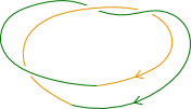
(b) The left-handed trefoil

Figure 17. Recovering a knot from a doubly pointed Heegaard diagram

Definition 4.8 (cf. Ozsváth and Szabó [25], Rasmussen [39]).

Suppose that $Y$ is a $\mathbb{Z}$-homology sphere, which implies that there is only one $\operatorname{Spin^{c}}$-structure on $Y$, which is torsion. Given a doubly pointed Heegaard diagram $\mathcal{H}=(\Sigma,\bm{\alpha},\bm{\beta},z,w)$ of $(Y,K)$, denote by $\mathcal{H}^{\prime}$ the pointed Heegaard diagram $\mathcal{H}=(\Sigma,\bm{\alpha},\bm{\beta},z)$ of $(Y,z)$. We define the hat and minus knot Floer chain complexes of $\mathcal{H}$,

$$\widehat{\operatorname{CFK}}(\mathcal{H}),\qquad\operatorname{CFK}^{\mathord{-}}(\mathcal{H}),$$

respectively as the chain complexes

$$\widehat{\operatorname{CF}}(\mathcal{H}^{\prime}),\qquad\operatorname{CF}^{\mathord{-}}(\mathcal{H}^{\prime}),$$

equipped with a relative $\mathbb{Z}$-filtration $A$, called the Alexander filtration, characterized by

$$A(\operatorname{\mathbf{x}})-A(\operatorname{\mathbf{y}})=n_{z}(B)-n_{w}(B)$$

for every $B\in\pi_{2}(\operatorname{\mathbf{x}},\operatorname{\mathbf{y}})$, where $n_{z}$ and $n_{w}$ denote the multiplicities of $z$ and $w$ in $B$ respectively. To ensure that $\operatorname{CFK}^{\mathord{-}}(\mathcal{H})$ is filtered, we set the filtration level of $U$ to be $-1$.

One can also define the infinity and plus knot Floer chain complexes $\operatorname{CFK}^{\infty}(\mathcal{H})$ and $\operatorname{CFK}^{+}(\mathcal{H})$ similarly.

Note that $H_{*}(\operatorname{CFK}^{\mathord{\circ}}(Y,K))$ is again $\operatorname{HF}^{\mathord{\circ}}(Y)$, since we must ignore the filtration when taking the homology. Given a $\mathbb{Z}$-filtered chain complex $\mathcal{C}=(C,\mathcal{F})$, recall that its associated graded object is the chain complex

$$\mathrm{g}\mathcal{C}=\bigoplus_{i\in\mathbb{Z}}\mathcal{F}_{i}C/\mathcal{F}_{i-1}C,$$

with an internal relative $\mathbb{Z}$-grading given by $i$. (Colloquially, in this context, we “erase” any term from the differential that strictly lowers the filtration.) In our setting, the internal $\mathbb{Z}$-grading on $\mathrm{gCFK}^{\mathord{\circ}}(\mathcal{H})$ is called its Alexander grading. (It continues to have a homological relative Maslov grading.) We define the knot Floer homology of $\mathcal{H}$ to be

$$\operatorname{HFK}^{\mathord{\circ}}(\mathcal{H})=H_{*}(\mathrm{gCFK}^{\mathord{\circ}}(\mathcal{H})).$$

When $Y=S^{3}$, we can fix an absolute Maslov grading $M$ on $\mathcal{S}(\mathcal{H}^{\prime})$ by requiring that

$$H_{*}(\widehat{\operatorname{CFK}}(\mathcal{H}))\cong\widehat{\operatorname{HF}}(S^{3})\cong\mathbb{F}$$

be concentrated in grading $0$. In this case, one can, with work, prove that the difference between the top and bottom Alexander gradings supported in $\widehat{\operatorname{HFK}}(\mathcal{H})$ is always $2g(K)$, where $g$ denotes the Seifert genus [24]; there is an absolute Alexander grading $A$ on $\mathcal{S}(\mathcal{H}^{\prime})$ characterized by the condition that the top Alexander grading be $g(K)$ and the bottom $-g(K)$.

Of course, the point is that these are knot invariants.

Theorem 4.9 (Ozsváth and Szabó [25, Theorem 3.1], Rasmussen [39, Theorem 1]).

Let $\mathcal{H}$ be a doubly pointed Heegaard diagram of $(Y,K)$, where $Y$ is a $\mathbb{Z}$-homology sphere and $K$ is null-homotopic. Then, the filtered, graded chain homotopy type of $\operatorname{CFK}^{\mathord{\circ}}(\mathcal{H})$ is an invariant of $(Y,K)$ for $\mathord{\circ}\in\{\raisebox{-4.30554pt}{$\widehat{\phantom{m}}$},-,+,\infty\}$ (resp. for $\mathord{\circ}\in\{\raisebox{-4.30554pt}{$\widehat{\phantom{m}}$},+\}$). Thus, we may write $\operatorname{CFK}^{\mathord{\circ}}(Y,K)$ for these chain complexes.

Example 4.10.

Using the doubly pointed Heegaard diagram in Figure 17(a), we can calculate the hat and minus knot Floer homologies of the left-handed trefoil to be

$$\widehat{\operatorname{HFK}}(S^{3},\overline{T}_{2,3})\cong\mathbb{F}^{\oplus 3},\qquad\operatorname{HFK}^{\mathord{-}}(S^{3},\overline{T}_{2,3})\cong\mathbb{F}[U]\oplus\faktor{\mathbb{F}[U]}{U}.$$

We conclude this discussion with some basic features of knot Floer homology:

• The graded Euler characteristic of $\widehat{\operatorname{HFK}}(S^{3},K)$ is defined to be

  $$\chi(\widehat{\operatorname{HFK}}(S^{3},K))=\sum_{M,A}(-1)^{M}t^{A}\cdot\operatorname{rk}_{\mathbb{F}}\widehat{\operatorname{HFK}}_{M}(S^{3},K,A),$$

  where $M$ and $A$ denote the Maslov and Alexander gradings respectively. A key feature of knot Floer homology is that this turns out to be the symmetrized Alexander polynomial [25]:

  $$\chi(\widehat{\operatorname{HFK}}(S^{3},K))=\Delta_{K}(t).$$

  (Recall that the Alexander polynomial is defined up to multiplication by a monomial; it can be symmetrized by requiring that $\Delta_{K}(t^{-1})=\Delta_{K}(t)$.)

• From $\operatorname{CFK}^{\infty}(S^{3},K)$, we can extract many other invariants of knots in $S^{3}$, e.g., $\tau(K)$ [22], $\epsilon(K)$ [7], $\Upsilon(K)$ [32], the torsion order of $\widehat{\operatorname{HFK}}(S^{3},K)$ [2, 1], etc. Many of these are powerful invariants, and some of them turn out to be concordance invariants.

• Heegaard Floer homology can be used to study contact $3$-manifolds (via open books), while knot Floer homology can be used for Legandrian and transverse knots. Namely, if a $3$-manifold $Y$ is equipped with a contact structure $\xi$, then there is an invariant $c(Y,\xi)\in\widehat{\operatorname{HF}}(-Y)$ [28, 8]; likewise, given a Legendrian knot $\Lambda\subset(Y,\xi)$, there are also invariants $\mathcal{L}(Y,\xi,\Lambda)\in\operatorname{HFK}^{\mathord{-}}(-Y,\Lambda)$ and $\widehat{\mathcal{L}}(Y,\xi,\Lambda)\in\widehat{\operatorname{HFK}}(-Y,\Lambda)$ [13, 30].

Knot Floer homology has a vast amount of applications, and can itself be the subject of an entire lecture series; the above is but a condensed introduction that inevitably misses many other important features.

4.6. Multi-pointed Heegaard and knot Floer homologies: Definition and relationship with grid homology

Previously, Heegaard diagrams $\mathcal{H}=(\Sigma,\bm{\alpha},\bm{\beta})$ have been assumed to have exactly $g(\Sigma)$ pairs of $\alpha$- and $\beta$-circles, and $\{z\}$ and $\{w\}$ have been singleton sets of points. In fact, we can work with more general multi-pointed Heegaard diagrams of the form

$$\mathcal{H}=(\Sigma_{g},\{\alpha_{1},\dotsc,\alpha_{g+n-1}\},\{\beta_{1},\dotsc,\beta_{g+n-1}\},\{z_{1},\dotsc,z_{n}\}),$$

possibly also with $\{w_{1},\dotsc,w_{n}\}$, for some $n\geq 1$. Such diagrams must satisfy the condition that each component of $\Sigma_{g}\setminus\bm{\alpha}$ contain exactly one $z_{i}$ (and also exactly one $w_{j}$ if $w_{j}$’s exist), and likewise for $\Sigma_{g}\setminus\bm{\beta}.$ For these multi-pointed Heegaard diagrams, we may define $\operatorname{CF}^{\mathord{\circ}}(\mathcal{H})$ or $\operatorname{CFK}^{\mathord{\circ}}(\mathcal{H})$ as before, except that we count holomorphic bigons in $\operatorname{Sym}^{g+n-1}(\Sigma)$ rather than in $\operatorname{Sym}^{g}(\Sigma)$.

The (filtered,) graded chain homotopy types of the resulting chain complexes turn out to coincide with those of the chain complexes defined with singly and doubly pointed Heegaard diagrams. In the proof, one considers an additional Heegaard move, quasi-(de)stabilization, where one adds (or subtracts) a pair of $\alpha$- and $\beta$-curves and a point $z_{i}$ (and $w_{j}$ if relevant).

For the story to come full circle, we note that grid diagrams are exactly multi-pointed Heegaard diagrams of knots $K\subset S^{3}$ that are nice in the sense of Sarkar and Wang [41].

Proposition 4.11.

Given a toroidal grid diagram $\mathbb{G}=(n,\mathbb{O},\mathbb{X})$ of $K\subset S^{3}$, the quintuple

$$\mathcal{H}=(T^{2},\{\text{horizontal circles}\},\{\text{vertical circles}\},\mathbb{O},\mathbb{X})$$

is a multi-pointed Heegaard diagram of $(S^{3},K)$.

Thus, the knot Floer chain complex can be computed by combinatorially counting domains of the correct index, which are empty rectangles.

Corollary 4.12 (Manolescu, Ozsváth, and Sarkar [15]).

Let $\mathbb{G}=(n,\mathbb{O},\mathbb{X})$ be a grid diagram of $K\subset S^{3}$. Then there is a chain homotopy equivalence

$$\mathcal{GC}^{-}(\mathbb{G})\simeq\operatorname{CFK}^{\mathord{-}}(S^{3},K)$$

of filtered, graded chain complexes over $\mathbb{F}[U]$.

C.-M. Michael Wong, University of Ottawa, Ottawa, Canada

E-mail address: mike.wong@uottawa.ca

Sarah Zampa, Budapest University of Technology and Economics, Budapest, Hungary

E-mail address: zampa.sarah@renyi.hu

References

- [1] Akram Alishahi and Eaman Eftekhary. Knot Floer homology and the unknotting number. Geom. Topol., 24(5):2435–2469, 2020.
- [2] Akram Alishahi and Eaman Eftekhary. Tangle Floer homology and cobordisms between tangles. J. Topol., 13(4):1582–1657, 2020.
- [3] Peter R Cromwell. Embedding knots and links in an open book i: Basic properties. Topology and its Applications, 64(1):37–58, 1995.
- [4] Andreas Floer. The unregularized gradient flow of the symplectic action. Comm. Pure Appl. Math., 41(6):775–813, 1988.
- [5] M. Gromov. Pseudo holomorphic curves in symplectic manifolds. Invent. Math., 82(2):307–347, 1985.
- [6] Kristen Hendricks and Ciprian Manolescu. Involutive Heegaard Floer homology. Duke Math. J., 166(7):1211–1299, 2017.
- [7] Jennifer Hom. The knot Floer complex and the smooth concordance group. Comment. Math. Helv., 89(3):537–570, 2014.
- [8] Ko Honda, William H. Kazez, and Gordana Matić. On the contact class in Heegaard Floer homology. J. Differential Geom., 83(2):289–311, 2009.
- [9] András Juhász. Cobordisms of sutured manifolds and the functoriality of link Floer homology. Adv. Math., 299:940–1038, 2016.
- [10] András Juhász, Dylan Thurston, and Ian Zemke. Naturality and mapping class groups in Heegard Floer homology. Mem. Amer. Math. Soc., 273(1338):v+174, 2021.
- [11] Robert Lipshitz. A cylindrical reformulation of Heegaard Floer homology. Geom. Topol., 10:955–1096, 2006.
- [12] Robert Lipshitz, Peter S. Ozsváth, and Dylan P. Thurston. Bordered Heegaard Floer homology. Mem. Amer. Math. Soc., 254(1216):viii+279, 2018.
- [13] Paolo Lisca, Peter Ozsváth, András I. Stipsicz, and Zoltán Szabó. Heegaard Floer invariants of Legendrian knots in contact three-manifolds. J. Eur. Math. Soc. (JEMS), 11(6):1307–1363, 2009.
- [14] Ciprian Manolescu and Peter Ozsváth. Heegaard Floer homology and integer surgeries on links. 2022.
- [15] Ciprian Manolescu, Peter Ozsváth, and Sucharit Sarkar. A combinatorial description of knot Floer homology. Ann. of Math. (2), 169(2):633–660, 2009.
- [16] Ciprian Manolescu, Peter Ozsváth, Zoltán Szabó, and Dylan Thurston. On combinatorial link Floer homology. Geom. Topol., 11:2339–2412, 2007.
- [17] András Némethi. On the Ozsváth-Szabó invariant of negative definite plumbed 3-manifolds. Geom. Topol., 9:991–1042, 2005.
- [18] András Némethi. Lattice cohomology of normal surface singularities. Publ. Res. Inst. Math. Sci., 44(2):507–543, 2008.
- [19] Yong-Geun O h. Floer cohomology of Lagrangian intersections and pseudo-holomorphic disks. I. Comm. Pure Appl. Math., 46(7):949–993, 1993.
- [20] Peter Ozsváth, András I. Stipsicz, and Zoltán Szabó. A spectral sequence on lattice homology. Quantum Topol., 5(4):487–521, 2014.
- [21] Peter Ozsváth and Zoltán Szabó. Absolutely graded Floer homologies and intersection forms for four-manifolds with boundary. Adv. Math., 173(2):179–261, 2003.
- [22] Peter Ozsváth and Zoltán Szabó. Knot Floer homology and the four-ball genus. Geom. Topol., 7:615–639, 2003.
- [23] Peter Ozsváth and Zoltán Szabó. On the Floer homology of plumbed three-manifolds. Geom. Topol., 7:185–224, 2003.
- [24] Peter Ozsváth and Zoltán Szabó. Holomorphic disks and genus bounds. Geom. Topol., 8:311–334, 2004.
- [25] Peter Ozsváth and Zoltán Szabó. Holomorphic disks and knot invariants. Adv. Math., 186(1):58–116, 2004.
- [26] Peter Ozsváth and Zoltán Szabó. Holomorphic disks and three-manifold invariants: properties and applications. Ann. of Math. (2), 159(3):1159–1245, 2004.
- [27] Peter Ozsváth and Zoltán Szabó. Holomorphic disks and topological invariants for closed three-manifolds. Ann. of Math. (2), 159(3):1027–1158, 2004.
- [28] Peter Ozsváth and Zoltán Szabó. Heegaard Floer homology and contact structures. Duke Math. J., 129(1):39–61, 2005.
- [29] Peter Ozsváth and Zoltán Szabó. Holomorphic triangles and invariants for smooth four-manifolds. Adv. Math., 202(2):326–400, 2006.
- [30] Peter Ozsváth, Zoltán Szabó, and Dylan Thurston. Legendrian knots, transverse knots and combinatorial Floer homology. Geom. Topol., 12(2):941–980, 2008.
- [31] Peter S. Ozsváth, András I. Stipsicz, and Zoltán Szabó. Grid homology for knots and links, volume 208 of Mathematical Surveys and Monographs. American Mathematical Society, Providence, RI, 2015.
- [32] Peter S. Ozsváth, András I. Stipsicz, and Zoltán Szabó. Concordance homomorphisms from knot Floer homology. Adv. Math., 315:366–426, 2017.
- [33] Peter S. Ozsváth, András I. Stipsicz, and Zoltán Szabó. Unoriented knot Floer homology and the unoriented four-ball genus. Int. Math. Res. Not. IMRN, (17):5137–5181, 2017.
- [34] Peter S. Ozsváth and Zoltán Szabó. Knot Floer homology and integer surgeries. Algebr. Geom. Topol., 8(1):101–153, 2008.
- [35] Peter S. Ozsváth and Zoltán Szabó. Knot Floer homology and rational surgeries. Algebr. Geom. Topol., 11(1):1–68, 2011.
- [36] Andrés Pedroza. A quick view of Lagrangian Floer homology. In Geometrical themes inspired by the N-body problem, volume 2204 of Lecture Notes in Math., pages 91–125. Springer, Cham, 2018.
- [37] Tim Perutz. A remark on Kähler forms on symmetric products of Riemann surfaces. 2008.
- [38] Timothy Perutz. Hamiltonian handleslides for Heegaard Floer homology. In Proceedings of Gökova Geometry-Topology Conference 2007, pages 15–35. Gökova Geometry/Topology Conference (GGT), Gökova, 2008.
- [39] Jacob Andrew Rasmussen. Floer homology and knot complements. ProQuest LLC, Ann Arbor, MI, 2003. Thesis (Ph.D.)–Harvard University.
- [40] Sucharit Sarkar. Moving basepoints and the induced automorphisms of link Floer homology. Algebr. Geom. Topol., 15(5):2479–2515, 2015.
- [41] Sucharit Sarkar and Jiajun Wang. An algorithm for computing some Heegaard Floer homologies. Ann. of Math. (2), 171(2):1213–1236, 2010.
- [42] Vladimir Turaev. Torsion invariants of -structures on -manifolds. Math. Res. Lett., 4(5):679–695, 1997.
- [43] Ian Zemke. Link cobordisms and absolute gradings on link Floer homology. Quantum Topol., 10(2):207–323, 2019.
- [44] Ian Zemke. Link cobordisms and functoriality in link Floer homology. J. Topol., 12(1):94–220, 2019.
- [45] Ian Zemke. The equivalence of lattice and Heegaard Floer homology. 2023.